Initial state radiation corrections to double charmonium production in one-photon electron-positron annihilation

Abstract

In this paper initial state radiation corrections to double production of charmonium mesons on one-photon electron-positron annihilation at center of mass energy $\sqrt{s}=10.6\,\text{GeV}$ are studied. It is shown, that these corrections have noticeable effect and must be taken into consideration.

I Introduction

Since the discovery of the so called charmonium mesons (that is mesons consisting of $c$- and $\bar{c}$-quarks, for example $J/\psi$, $\psi(2S)$ or $\eta_{c}$) in 1974 Aubert et al. (1974); Augustin et al. (1974) they play a significant role in our understanding of quantum chromodynamics (QCD). Production of charmonium requires creation of heavy $c\bar{c}$ pair with the energy greater than $2m_{c}$ where QCD coupling constant is small enough to use perturbation theory. However, the subsequent hadronization probes much smaller mass scales of order $m_{c}v^{2}$, where $v$ is typical velocity of $c$ quark in the charmonium rest frame. For $J/\psi$, $m_{c}v^{2}$ is numerically of order $\Lambda_{\rm QCD}$, so the production processes are sensitive to nonperturbative physics as well. Charmonium mesons are also very interesting from the experimental point of view, since the narrow resonances can easily be separated from the background.

In 1986 Caswell and Lepage have proposed the Non-Relativistic Quantum Chromodynamics model (NRQCD) Caswell and Lepage (1986); Bodwin et al. (1995). This model exploits the fact that the velocity $v$ of the heavy quark in the charmonium rest frame is small in comparison with the speed of light and all physical quantities can be expressed as the series in this small velocity and electromagnetic and strong coupling constants $\alpha$ and $\alpha_{s}$. Matrix elements of the four-fermion operators, used in this theory, can be determined phenomenologically. Both inclusive and exclusive production of charmonium mesons and their decays were studied using this theory Braaten and Chen (1996); Cho and Leibovich (1996); Bodwin and Petrelli (2002); Braaten and Lee (2003); Bodwin et al. (2003a); Hagiwara et al. (2003); Wang et al. (2002).

New difficulties have arisen as a result of recent measurements of inclusive charmonium production in $e^{+}e^{-}$ collisions by Belle and BABAR collaborations Aubert et al. (2001); Abe et al. (2002a). Their results were about an order of magnitude higher, than the predictions based on NRQCD or other models Kiselev et al. (1994); Braaten and Chen (1996); Berezhnoy and Likhoded (2003); Leibovich et al. (2003); Luchinsky (2003a).

Another difference has arisen in studying the exclusive production of pair of charmonium mesons. For example, the NRQCD results for $J/\psi\eta_{c}$ production is Braaten and Lee (2003)

$$\sigma_{0} = \sigma\left(e^{+}e^{-}\to\gamma^{*}\to J/\psi\eta_{c}\right)=2.31\,\text{fb}$$

and Belle results Abe et al. (2002b) are an order of magnitude higher. One of the possible explanations of this difference was proposed in Bodwin et al. (2003b). The authors assumed that some of the Belle’s $J/\psi\eta_{c}$ signals could actually be the double production of $J/\psi$ meson with subsequent decay $J/\psi\to\eta_{c}\gamma$ and presented the value

$$\sigma\left(e^{+}e^{-}\to 2\gamma^{*}\to 2J/\psi\right) = 8.7\,\text{fb}.$$

Later in Braaten and Lee (2003); Luchinsky (2003b) it was shown that due to relativistic and higher order QCD corrections the cross section should be about 4 times smaller and the question of the difference between theory and experiment remains open.

In this paper I propose that this difference can be explained by the initial state radiation corrections. Indeed, the naive estimate of the effect of these corrections gives us the result

$$\sigma = \sigma\left(e^{+}e^{-}\to J/\psi\eta_{c}\gamma\right)\sim\alpha\log\frac{s}{m_{e}^{2}}\sigma_{0}$$

and the suppression caused by additional factor $\alpha$ will be compensated by large logarithm $\log{s/m_{e}^{2}}$. Another reason is that cross section of the reaction $e^{+}e^{-}\to J/\psi\eta_{c}$ as a function of center of mass energy $\sqrt{s}$ has a narrow peak near $\sqrt{s}\approx 6.5\,\,\text{GeV}$, where $\sigma\left(e^{+}e^{-}\to J/\psi\eta_{c}\right)\approx 30\,\text{fb}$ and by emitting a hard photon we can return to this region.

The rest of this paper is organized as follows. In the next section I give the diagrams and matrix element for the process under consideration. In section III the method of calculation of the total cross section is described. Finally, distributions over vector charmonium energy and scattering angle are presented.

II Matrix element

The diagrams for the process $e^{-}\left(k_{1}\right)e^{+}\left(k_{2}\right)\to J/\psi\left(p_{1},E\right)\eta_{c}\left(p_{2}\right)\gamma\left(k,\epsilon\right)$ are shown on figure 1. The vertex of the transition of virtual photon with momentum $\hat{p}$ and its square $\hat{s}=\hat{p}^{2}$ into pair of charmonium states, denoted here by filled circle, was calculated in Braaten and Lee (2003). Some of the diagrams of this transition are shown on figure 2, the others can be obtained from them by permutations. One can also add electromagnetic diagrams by replacing the gluon line in figure 2(a) by photon, but they are suppressed by the factor $\alpha/\alpha_{s}$ and will not be considered here. On the other hand, as it was shown in Braaten and Lee (2003) the purely electromagnetic resonance diagrams (for example, the diagram 2(b)) must be included. The reason for this is that the additional factor $\alpha$ is compensated by $r^{2}=4M^{2}/\hat{s}$, where $M=2m_{c}$ is the mass of the charmonium meson (the difference between $J/\psi$ and $\eta_{c}$ masses is neglected) and $m_{c}$ is $c$-quark mass.

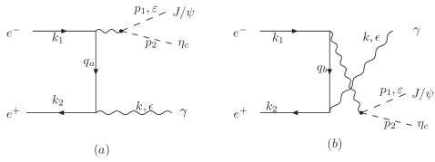
Figure 1: Diagrams for $e^{+}e^{-}\to J/\psi\eta_{c}\gamma$.

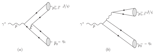
Figure 2: Some diagrams for the transition of a virtual photon into charmonium pair. Other diagrams can be obtained from theses by permutations.

The analytical expression for the $\gamma J/\psi\eta_{c}$ vertex was found to be

$$J_{\mu} = \left<J/\psi\left(p_{1},\varepsilon\right)\eta_{c}\left(p_{2}\right)\left|\bar{c}\gamma_{\mu}c\right|0\right>=$$

$$= iA\epsilon_{\mu\nu\alpha\beta}\varepsilon^{\nu}p_{1}^{\alpha}p_{2}^{\beta},$$

where $\varepsilon$ is the polarization vector of the vector charmonium $J/\psi$, the coefficient $A$ is

$$A = \frac{128\pi\alpha_{s}}{\hat{s}^{2}}\sqrt{O_{\psi}O_{\eta}}\left(\frac{N_{c}^{2}-1}{2N_{c}^{2}}+\frac{e_{c}^{2}\alpha}{N_{c}\alpha_{s}}-\frac{1}{r^{2}}\frac{e_{c}^{2}\alpha}{\alpha_{s}}\right),$$

$N_{c}=3$ is the number of colors, $e_{c}=2/3$ is the charge of the $c$ quark (in the units of the elementary charge $e$), and the constants

$$O_{\psi} = \left<O_{1}\right>_{J/\psi},\qquad O_{\eta}=\left<O_{1}\right>_{\eta_{c}}$$

are the matrix elements of the NRQCD probability factors. These constants can be determined from the experimental data on $J/\psi$ and $\eta_{c}$ decay widths Braaten and Lee (2003):

$$O_{\psi} = \frac{27}{32\pi\alpha^{2}}\Gamma\left(J/\psi\to e^{+}e^{-}\right)M^{2}\left(1-\frac{8}{3}\frac{\alpha_{s}}{\pi}\right)^{-2},$$

$$O_{\eta} = \frac{81}{128\pi\alpha^{2}}\Gamma\left(\eta_{c}\to\gamma\gamma\right)\left(1-\frac{2-\pi^{2}}{6}\frac{\alpha_{s}}{\pi}\right)^{-2}.$$

Using the table data on particle decay widths Groom et al. (2000) we get the numerical values of probability factors, that will be used in this paper:

$$O_{\psi} = 0.335\,\text{GeV}^{3},$$

$$O_{\eta} = 0.297\,\text{GeV}^{3}.$$

The matrix element corresponding to the diagrams shown on figure 1 is

$${\cal M} = \frac{e_{c}e^{3}}{\hat{s}}\epsilon^{\mu}J^{\nu}\bar{v}\left(k_{2}\right)\left\{\frac{1}{q_{a}^{2}}\gamma_{\nu}\hat{q}_{a}\gamma_{\mu}+\right.$$ (1)

$$\left.\frac{1}{q_{b}^{2}}\gamma_{\mu}\hat{q}_{b}\gamma_{\nu}\right\}u\left(k_{1}\right),$$

where $k_{1}$ and $k_{2}$ are electron and positron momenta (the mass of the electron $m_{e}$ is neglected wherever it is possible), $k$ is the momentum of the final state photon, $\epsilon_{\mu}$ is its polarization vector, $q_{a}=k_{1}-k$ and $q_{b}=k-k_{2}$ are the momentum transfer in this two diagrams. The cross section found from (1) and equals to

$$\sigma = \frac{1}{2048\pi^{7}\left(k_{1}k_{2}\right)}\int d\Phi_{3}\left(k_{1}+k_{2};p_{1},p_{2},k\right)\sum\left|{\cal M}\right|^{2},$$

where summation is performed over polarizations of initial and final particles and for the Lorentz-invariant phase space the notation

$$d\Phi_{n}\left(P;p_{1},\ldots,p_{n}\right) = \delta\left(P-\sum\limits_{i=1}^{n}p_{i}\right)\prod\limits_{i=1}^{n}\frac{d^{3}p_{i}}{2E_{i}}$$ (2)

is used.

III Total cross section

The Lorentz-invariant phase space (2) satisfies the recursion relation

$$d\Phi_{3}\left(k_{1}+k_{2};p_{1},p_{2},k\right) = d\hat{s}d\Phi_{2}\left(k_{1}+k_{2};\hat{p},k\right)$$

$$\times d\Phi_{2}\left(\hat{s};p_{1},p_{2}\right),$$

where $\hat{p}=p_{1}+p_{2}$ is the momentum of the virtual photon, $\hat{s}=\hat{p}^{2}=s-2\sqrt{s}E_{k}$, and $E_{k}$ is the final state photon energy in the laboratory frame. Leaving only the integration over $E_{k}$ we get the differential cross section

$$\frac{d\sigma}{d\hat{s}} = \frac{32768\pi^{2}\alpha^{3}}{19683}\frac{O_{\psi}O_{\eta}}{s^{2}}\left(1-\frac{4M^{2}}{\hat{s}}\right)^{3/2}\times$$

$$\times \frac{(2\alpha\hat{s}-4M^{2}(\alpha+2\alpha_{s}))^{2}}{\hat{s}^{4}}\times$$

$$\times \left(2\frac{s^{2}+\hat{s}^{2}}{s-\hat{s}}\frac{\text{arctanh}\,\beta_{e}}{\beta_{e}}-s+\hat{s}\right).$$

From this equation one can easily notice two important items:

• the cross section is enhanced by the factor $\text{arctanh}\,\beta_{e}\sim\log s/m_{e}^{2}$ as it was states in the introduction,

• total cross section actually diverges in the limit $\hat{s}\approx s$. This fact is the familiar infrared divergence caused by the emission of the soft photon, where one can not use the perturbation theory. To avoid this divergence one must put the cutoff $\delta_{\epsilon}$ on the energy of the photon:

  $$E_{k} > \delta_{\epsilon}.$$

Figure 3: Distribution over final state photon energy

The plot for differential cross section $d\sigma/dE_{k}$ is presented on figure 3. As stated above, in the limit of small photon energy it grows to infinity and one should put the cutoff. The bump in the region $E_{k}\approx 3\,\text{GeV}$ corresponds to $\sqrt{\hat{s}}\approx 6.5\,\text{GeV}$, where the cross section of the process $\gamma^{*}\to J/\psi\eta_{c}$ is maximal.

Values of total cross section for some cutoff photon energies are:

$$\sigma \approx 2.84\,\text{fb}\quad\rm{for\ }\delta_{\epsilon}=1\,\text{MeV},$$

$$\sigma \approx 2.234\,\text{fb}\quad\rm{for\ }\delta_{\epsilon}=10\,\text{MeV},$$

$$\sigma \approx 1.72\,\text{fb}\quad\rm{for\ }\delta_{\epsilon}=100\,\text{MeV}.$$

It is easily seen, that by the order of magnitude these cross sections equals to the cross section of the base process $e^{+}e^{-}\to\gamma^{*}\to J/\psi\eta_{c}$, so the initial state radiation corrections should be taken into account.

IV Differential cross section

For the calculation of the differential cross section over the vector charmonium energy it is convenient to introduce dimensionless variables according to formula’s

$$z_{k,1,2} = \frac{2E_{k,1,2}}{\sqrt{s}},$$

$$\mu = \frac{2M}{\sqrt{s}},$$

$$x_{k,1,2} = \cos\theta_{k,1,2},$$

$$y_{k,1,2} = \sqrt{1-x_{k,1,2}^{2}}\,,$$

where $E_{1}$, $E_{2}$ and $E_{k}$ are the energies of vector and pseudoscalar charmonia and photon in the center of mass frame respectively; $\theta_{1}$, $\theta_{2}$ and $\theta_{k}$ are the angles between the momentum of the initial electron and the momenta of these final particles. These variables take the values in the regions

$$x_{1},x_{k} \in [-1;1],$$

$$z_{1} \in [\mu;1],$$

$$z_{k} \in [z_{k}^{m};z_{k}^{M}],$$

where minimum and maximum values of $z_{k}$ are

$$z_{k}^{m,M} = \frac{2(1-z_{1})}{2-z_{1}[1-\beta(x_{1}x_{k}\pm y_{1}y_{k})]}.$$

In the terms of these variables the squared matrix element and Lorentz-invariant phase space take the form

$$\left|{\cal M}\right|^{2} = \frac{13417728\alpha^{3}}{6561\mu^{4}}\frac{O_{\psi}O_{\eta}}{s^{4}}\frac{(3\alpha_{s}\mu-\alpha(3-3z_{k}-\mu^{2}))^{2}}{z_{k}^{2}(1-z_{k})^{5}(1-\beta_{e}^{2}x_{k}^{2})}\left\{\rule{0.0pt}{14.22636pt}4\left(2-\mu^{2}-2z_{1}+(1+\beta^{2}x_{1}^{2})z_{1}^{2}\right)-\right.$$

$$4\left(4-\mu^{2}-3\left(3+\beta x_{1}x_{k}\right)z_{1}+\left(1+\beta^{2}x_{1}^{2}\right)z_{1}^{2}\right)z_{k}+$$

$$\left(2\left(5-2z_{1}\left(1-\beta x_{1}x_{k}\right)+x_{k}^{2}\right)-\mu^{2}\left(1+x_{k}^{2}\right)\right)z_{k}^{2}-$$

$$\left.\rule{0.0pt}{14.22636pt}2\left(1+x_{k}^{2}\right)z_{k}^{3}\right\},$$

$$d\Phi_{3}\left(k_{1}+k_{2};p_{1},p_{2},k\right) = \frac{\pi s}{16}\frac{\beta z_{1}z_{k}}{1-z_{1}}\sqrt{\frac{z_{k}^{M}z_{k}^{m}}{(z_{k}^{M}-z_{k})(z_{k}-z_{k}^{m})}}dz_{1}dx_{1}dz_{k}dx_{k},$$

where $\beta=\sqrt{1-M^{2}/E_{1}^{2}}=\sqrt{1-\mu^{2}/z_{1}^{2}}$ is the velocity of the vector charmonium meson and $\beta_{e}=\sqrt{1-4m_{e}^{2}/s}$ is the velocity of the initial electron in the laboratory frame (this is the only place where I have to leave the non-vanishing electron mass).

For integration of the differential cross section over $z_{k}$ it is possible to use the residue technique. The only $d^{4}\sigma/dx_{1}dz_{1}dx_{z}dz_{k}$ poles are $z_{k}=0,1$ in , so we can write

$$\frac{d^{3}\sigma}{dx_{1}dz_{1}dx_{k}} = i\pi\sum\limits_{z_{k}=0,1}{\text{res}\,}\frac{d^{4}\sigma}{dx_{1}dz_{1}dx_{k}dz_{k}}.$$

The residue at $z_{k}=1$ is too lengthy to be presented here, but the residue at $z_{k}=0$, that plays most important role for $z_{1}\approx 1$ (that is in the limit of maximal vector charmonium energy) and $x_{1}\neq\pm 1$ it is rather compact. In this limit we have

$$\frac{d^{2}\sigma}{dz_{1}dx_{1}} = S(z_{1})\left[1+B(z_{1})x_{1}^{2}\right],$$

$$S(z_{1}) = \frac{262144\pi^{2}\alpha^{3}\beta}{6561\mu^{4}}\frac{O_{\psi}O_{\eta}}{s^{4}}\frac{\text{arctanh}\,\beta_{e}}{\beta_{e}}z_{1}\times$$

$$\times \frac{(2-\mu^{2}-2z_{1}+z_{1}^{2})(3\alpha_{s}\mu^{2}-\alpha(3-\mu^{2}))^{2}}{1-z_{1}},$$

$$B(z_{1}) = \frac{\beta^{2}z_{1}^{2}}{2-\mu^{2}-2z_{1}+z_{1}^{2}}.$$

The integration over all other variables was performed numerically.

The distribution over vector charmonium energy is shown on figure 4. In the limit of maximal vector charmonium energy ($z_{1}\approx 1$) this curve grows to infinity corresponding to analogous grows int the distribution over photon energy shown on figure 3.

The distributions over scattering angle for different values of $\delta_{\epsilon}$ are shown on figure 5. This form of distribution is usual for color-singlet charmonium production.

Figure 4: Distribution over vector charmonium energy.

Figure 5: Distribution over scattering angle for $\delta_{\epsilon}=1\,\text{MeV}$ (solid line), $\delta_{\epsilon}=10\,\text{MeV}$ (dashed line), and $\delta_{\epsilon}=100\,\text{MeV}$ (dotted line)

References

Aubert et al. (1974)
J. J. Aubert
et al., Phys. Rev. Lett.
33, 1404 (1974).
Augustin et al. (1974)
J. E. Augustin
et al., Phys. Rev. Lett.
33, 1406 (1974).
Caswell and Lepage (1986)
W. E. Caswell and
G. P. Lepage,
Phys. Lett. B167,
437 (1986).
Bodwin et al. (1995)
G. T. Bodwin,
E. Braaten, and
G. P. Lepage,
Phys. Rev. D51,
1125 (1995), eprint hep-ph/9407339.
Braaten and Chen (1996)
E. Braaten and
Y.-Q. Chen,
Phys. Rev. Lett. 76,
730 (1996), eprint hep-ph/9508373.
Cho and Leibovich (1996)
P. L. Cho and
A. K. Leibovich,
Phys. Rev. D54,
6690 (1996), eprint hep-ph/9606229.
Bodwin and Petrelli (2002)
G. T. Bodwin and
A. Petrelli,
Phys. Rev. D66,
094011 (2002), eprint hep-ph/0205210.
Braaten and Lee (2003)
E. Braaten and
J. Lee,
Phys. Rev. D67,
054007 (2003), eprint hep-ph/0211085.
Bodwin et al. (2003a)
G. T. Bodwin
et al., Phys. Rev.
D67, 054023
(2003a), eprint hep-ph/0205352.
Hagiwara et al. (2003)
K. Hagiwara
et al., Phys.Lett.
B570, 39 (2003),
eprint hep-ph/0305102.
Wang et al. (2002)
P. Wang et al.
(2002), eprint hep-ex/0210062.
Aubert et al. (2001)
B. Aubert et al.,
Phys.Rev.Lett. 87,
162002 (2001), eprint hep-ex/0106044.
Abe et al. (2002a)
K. Abe et al.,
Phys.Rev.Lett. 88,
052001 (2002a),
eprint hep-ex/0110012.
Kiselev et al. (1994)
V. V. Kiselev,
A. K. Likhoded,
and M. V.
Shevlyagin, Phys. Lett.
B332, 411 (1994),
eprint hep-ph/9408407.
Berezhnoy and Likhoded (2003)
A. V. Berezhnoy
and A. K.
Likhoded (2003), eprint hep-ph/0303145.
Leibovich et al. (2003)
A. Leibovich
et al., Phys.Rev.
D68, 094011
(2003), eprint hep-ph/0306139.
Luchinsky (2003a)
A. V. Luchinsky
(2003a), eprint hep-ph/0305253.
Abe et al. (2002b)
K. Abe et al.,
Phys.Rev.Lett. 89,
142001 (2002b),
eprint hep-ex/0205104.
Bodwin et al. (2003b)
G. T. Bodwin,
J. Lee, and
E. Braaten,
Phys. Rev. Lett. 90,
162001 (2003b),
eprint hep-ph/0212181.
Luchinsky (2003b)
A. V. Luchinsky
(2003b), eprint hep-ph/0301190.
Groom et al. (2000)
D. E. Groom et al.
(Particle Data Group), Eur. Phys.
J. C15, 1
(2000).