The branching ratio $R_{b}$ in the littlest Higgs model

Abstract

In the context of the littlest Higgs(LH) model, we study the contributions of the new particles to the branching ratio $R_{b}$. We find that the contributions mainly dependent on the free parameters $f$, $c^{\prime}$ and $x_{L}$. The precision measurement value of $R_{b}$ gives severe constraints on these free parameters.

PACS number: 12.60.Cn, 14.80.Cp, 12.15.Lk

I. Introduction

It is well know that most of the electroweak oblique and QCD corrections to the $Z\rightarrow b\overline{b}$ branching ratio $R_{b}$ cancel between numerator and denominator, $R_{b}$ is very sensitive to the new physics(NP) beyond the standard model(SM). The precision experimental value of $R_{b}$ may give a severe constraint on the NP[1]. Thus, it is very important to study the $Z\rightarrow b\overline{b}$ process in extensions of the SM and pursue the resulting implications.

Little Higgs models[2,3,4] provide a new approach to solve the hierarchy between the $TeV$ scale of possible NP and the electroweak scale, $\nu=246GeV=(\sqrt{2}G_{F})^{-1/2}$. In these models, at least two interactions are needed to explicitly break all of the global symmetries, which forbid quadratic divergences in the Higgs mass at one-loop. Electroweak symmetry breaking(EWSB) is triggered by a Coleman-Weinberg potential, which is generated by integrating out the heavy degrees of freedom. In this kind of models, the Higgs boson is a pseudo-Goldstone boson of a global symmetry which is spontaneously broken at some higher scale $f$ by an vacuum expectation value(VEV) and thus is naturally light. A general feature of this kind of models is that the cancellation of the quadratic divergences is realized between particles of the same statistics.

Little Higgs models are weakly interaction models, which contain extra gauge bosons, new scalars and fermions, apart from the SM particles. These new particles might produce characteristic signatures at the present and future collider experiments[5,6,7]. Since the extra gauge bosons can mix with the SM gauge bosons $W$ and $Z$, the masses of the SM gauge bosons $W$ and $Z$ and their couplings to the SM particles are modified from those in the SM at the order of $\frac{\nu^{2}}{f^{2}}$. Thus, the precision measurement data can give severe constraints on this kind of models[5,8,9].

Aim of this paper is to consider the $Z\rightarrow b\overline{b}$ branching ratio $R_{b}$ in the context of the littlest Higgs(LH) model[2] and see whether the new particles predicted by the LH model can give significant contributions to $R_{b}$. We find that, compare the calculated value of $R_{b}$ with the experimental measured value, the precision data can give severe constraint on the free parameters of the LH model.

The LH model has been extensively described in literature. However, in order to clarify notation which is relevant to our calculation, we will simply review the LH model in section II. In section III, we discuss the effects of the new gauge bosons on the branching ratio $R_{b}$. We calculate the contributions of the top quark $t$ and vector-like quark $T$ to $R_{b}$ via the couplings $W\overline{t}b,W\overline{T}b,W^{\prime}\overline{t}b$ and $W^{\prime}\overline{T}b$ in section IV. The contributions of the new scalars to $R_{b}$ are studied in section V. Discussions and conclusions are given in section VI.

II. Littlest Higgs model

The LH model[2] is embedded into a non-linear $\sigma$ model with the coset space of $SU(5)/SO(5)$. At the scale $\Lambda_{s}\sim 4\pi f$, the global $SU(5)$ symmetry is broken into its subgroup $SO(5)$ via a VEV of order $f$, resulting in 14 Goldstone bosons. The effective field theory of these Goldstone bosons is parameterized by a non-linear $\sigma$ model with gauge symmetry $[SU(2)\times U(1)]^{2}$, spontaneously broken down to its diagonal subgroup $SU(2)\times U(1)$, identified as the SM electroweak gauge group. Four of these Goldstone bosons are eaten by the broken gauge generators, leaving 10 states that transform under the SM gauge group as a doublet $H$ and a triplet $\Phi$. A new charge $2/3$ quark $T$ is also needed to cancel the divergences from the top quark loop.

The effective non-linear Lagrangian invariant under the local gauge group $[SU(2)_{1}\times U(1)_{1}]\times[SU(2)_{2}\times U(1)_{2}]$, which can be written as[5,9]:

$$\pounds_{eff}=\pounds_{G}+\pounds_{F}+\pounds_{Y}+\pounds_{\Sigma}-V_{CW},$$ (1)

where $\pounds_{G}$ consists of the pure gauge terms, which can give the $3-$ and $4-$particle interactions among the $SU(2)$ gauge bosons and the couplings of the $U(1)$ gauge bosons to the $SU(2)$ gauge bosons. The fermion kinetic term $\pounds_{F}$ can give the couplings of the gauge bosons to fermions. The couplings of the scalars $H$ and $\Phi$ to fermions can be derived from the Yukawa interaction term $\pounds_{Y}$. In the LH model, the global symmetry prevents the appearance of a Higgs potential at tree level. The effective Higgs potential, the Coleman-Weinberg potential $V_{CW}$[10], is generated at one-loop and higher orders due to interactions with gauge bosons and fermions, which can induce to EWSB by driving the Higgs mass squared parameter negative. $\pounds_{\Sigma}$ consists of the $\sigma$ model terms of the LH model. The scalar $\Sigma$ field can be written as:

$$\Sigma=e^{i\Pi/f}\langle\Sigma_{0}\rangle e^{i\Pi^{T}/f}=e^{2i\Pi/f}\langle\Sigma_{0}\rangle$$ (2)

with $\langle\Sigma_{0}\rangle\sim f$ which generates masses and mixing between the gauge bosons. The ten pseudo-Goldstone bosons can be parameterized as:

$$\Pi=\left(\begin{array}[]{ccc}0&H^{+}/\sqrt{2}&\Phi^{+}\\ H/\sqrt{2}&0&H^{\ast}/\sqrt{2}\\ \Phi&H^{T}/\sqrt{2}&0\end{array}\right).$$ (3)

Where $H$ is identified as the SM Higgs doublet, $H=(H^{+},H^{0})$, and $\Phi$ is a complex $SU(2)$ triplet with hypercharge $Y=2$,

$$\Phi=\left(\begin{array}[]{cc}\Phi^{++}&\Phi^{+}/\sqrt{2}\\ \Phi^{+}/\sqrt{2}&\Phi^{0}\end{array}\right).$$ (4)

The kinetic terms of the scalar $\Sigma$ field are given by

$$\pounds_{\Sigma}=\frac{f^{2}}{8}Tr\{(D_{\mu}\Sigma)(D^{\mu}\Sigma)^{+}\},$$ (5)

where the covariant derivative of the $\Sigma$ field is defined as:

$$D_{\mu}\Sigma=\partial_{\mu}\Sigma-i\sum_{j}[g_{j}W^{a}_{j}(Q^{a}_{j}\Sigma+\Sigma Q^{aT}_{j})+g_{j}^{\prime}B_{j}(Y_{j}\Sigma+\Sigma Y_{j}^{T})],$$ (6)

where $g_{j},g^{\prime}_{j}$ are the gauge coupling constants, $W_{j},B_{j}$ are the gauge bosons, $Q_{j}^{a}$ and $Y_{j}$ are the generators of gauge transformations. The gauge boson mass eigen-states are given by

$$\begin{array}[]{cc}W=sW_{1}+cW_{2},&W^{\prime}=-cW_{1}+sW_{2},\\ B=s^{\prime}B_{1}+c^{\prime}B_{2},&B^{\prime}=-c^{\prime}B_{1}+s^{\prime}B_{2}\end{array}$$ (7)

with the cosines of two mixing angles,

$$c=\frac{g_{1}}{\sqrt{g_{1}^{2}+g_{2}^{2}}},\hskip 56.9055ptc^{\prime}=\frac{g^{\prime}_{1}}{\sqrt{g^{\prime 2}_{1}+g^{\prime 2}_{2}}}.$$ (8)

The SM gauge coupling constants are $g=g_{1}s=g_{2}c$ and $g^{\prime}=g^{\prime}_{1}s^{\prime}=g^{\prime}_{2}c^{\prime}$.

From the effective non-linear Lagrangian ${\cal L}$, one can derive the mass and coupling expressions of the gauge bosons, scalars and the fermions, which have been extensively discussed in Refs.[5,9]. The mass spectrum of the LH model and the coupling forms which are related our calculations are summarized in appendix A , B and C, respectively.

III. New gauge bosons and the $Z\rightarrow b\overline{b}$ branching ratio $R_{b}$

1. Corrections of new physics to the $Z\rightarrow b\overline{b}$ branching ratio $R_{b}$

In general, the effective $Z\rightarrow b\overline{b}$ vertex can be written as:

$$[g_{L}^{b}\overline{b}_{L}\gamma^{\mu}b_{L}+g_{R}^{b}\overline{b}_{R}\gamma^{\mu}b_{R}]\cdot Z^{\mu}$$ (9)

with the form factors $g_{L}^{b}$ and $g_{R}^{b}$:

$$g_{L}^{b} = g_{L}^{b,SM}+\delta g_{L}^{b}=\frac{e}{S_{W}C_{W}}(-\frac{1}{2}+\frac{1}{3}S_{W}^{2})+\delta g_{L}^{b},$$

$$g_{R}^{b} = g_{R}^{b,SM}+\delta g_{R}^{b}=\frac{e}{S_{W}C_{W}}(\frac{1}{3}S_{W}^{2})+\delta g_{R}^{b}.$$ (10)

Where $S_{W}=\sin\theta_{W}$, $\theta_{W}$ is the Weinberg angle. $\delta g_{L}^{b}$ and $\delta g_{R}^{b}$ represent the corrections of NP to the left-handed and right-handed $Zb\overline{b}$ couplings, respectively. Certainly, the corrections of NP to the $Zb\overline{b}$ couplings $g_{L}^{b}$ and $g_{R}^{b}$ may give rise to one additional form factor, proportional to $\sigma^{\mu\nu}q^{\nu}$. However, its contributions to $R_{b}$ are very small and can be ignored[1].

The branching ratio $R_{b}$ can be written as:

$$R_{b}=\frac{\Gamma_{b}}{\Gamma_{h}}=\frac{\Gamma_{b}}{3\Gamma_{b}+2\Gamma_{c}}.$$ (11)

Here $\Gamma_{c}$ is the width of the process $Z\rightarrow c\overline{c}$. The partial decay width, $\Gamma_{q}$, of the $Z\rightarrow q\overline{q}$ decay($q=u,d,c,s$, and $b$) is given as[11]:

$$\Gamma_{q}=6\Gamma_{0}(1+\frac{\alpha_{s}}{\pi})[(g_{L}^{q})^{2}+(g_{R}^{q})^{2}],$$ (12)

with $\Gamma_{0}=\frac{G_{F}m_{Z}^{3}}{24\sqrt{2}\pi}$. The factor $\frac{\alpha_{s}}{\pi}$ contain contributions from the find state gluons and photons. In above equation, the masses of the final quarks are assumed to be negligible.

Since the branching ratio $R_{b}$ is the ratio between two hadronic widths, $R_{b}$ is almost independent of the EW oblique and QCD corrections because of the near cancellation of these corrections between the numerator and the denominator. The remaining ones are absorbed in the definition of the renormalized coupling parameters $\alpha$ and $S_{W}$, up to terms of high order in the electroweak corrections[12]. Thus, $R_{b}$ is very sensitive to the NP beyond the SM. The correction of NP to $R_{b}$ can be written as:

$$\delta R_{b} = R_{b}-R_{b}^{SM}=\frac{\Gamma_{b}^{SM}+\delta\Gamma_{b}}{\Gamma_{h}^{SM}+\delta\Gamma_{h}}-\frac{\Gamma_{b}^{SM}}{\Gamma_{h}^{SM}}\approx(\frac{\delta\Gamma_{b}}{\Gamma_{b}}-\frac{\delta\Gamma_{h}}{\Gamma_{h}})R_{b}^{SM}$$ (13)

$$= R_{b}^{SM}\{\frac{2(g_{L}^{b}\delta g_{L}^{b}+g_{R}^{b}\delta g_{R}^{b})}{(g_{L}^{b})^{2}+(g_{R}^{b})^{2}}-\frac{4(g_{L}^{c}\delta g_{L}^{c}+g_{R}^{c}\delta g_{R}^{c})+6(g_{L}^{b}\delta g_{L}^{b}+g_{R}^{b}\delta g_{R}^{b})}{2[(g_{L}^{c})^{2}+(g_{R}^{c})^{2}]+3[(g_{L}^{b})^{2}+(g_{R}^{b})^{2}]}\}.$$

In above equation, we have neglected the terms of $O[(\delta g_{L,R}^{q})^{2}]$. In the next subsection, we will study the corrections of the new gauge bosons predicted by the LH model to the branching ratio $R_{b}$.

2. The extra gauge bosons and the branching ratio $R_{b}$

The LH model predicts the existence of the extra gauge bosons, such as $W^{\prime},Z^{\prime}$ and $B^{\prime}$. These new particles can generate corrections to the branching ratio $R_{b}$ via mixing with the SM gauge bosons and the coupling to the SM fermions. The corrections to $R_{b}$ mainly come from three sources: (1) the modifications of the relations between the SM parameters and the precision electroweak input parameters, which come from the mixing of the heavy $W^{\prime}$ boson to the couplings of the charge current and from the contributions of the current to the equations of motion of the heavy gauge bosons, (2) the correction terms to the $Zb\overline{b}$ couplings $g_{L}^{b}$ and $g_{R}^{b}$ coming from the mixing between the extra gauge boson $Z^{\prime}$ and the SM gauge boson $Z$, (3) the neutral gauge bosons $Z^{\prime}$ exchange and $B^{\prime}$ exchange. In the LH model, the relation between the Fermi coupling constant $G_{F}$, the gauge boson $Z$ mass $m_{Z}$ and the fine structure coupling constant $\alpha(m_{Z})$ can be written as[9]:

$$\frac{G_{F}}{\sqrt{2}}=\frac{\pi\alpha}{2\sqrt{2}m_{Z}^{2}S_{W}^{2}C_{W}^{2}}[1-\frac{g}{G_{F}}\frac{c}{s}(c^{2}-s^{2})\frac{\nu^{2}}{f^{2}}+2c^{4}\frac{\nu^{2}}{f^{2}}-\frac{5}{4}(c^{\prime 2}-s^{\prime 2})^{2}\frac{\nu^{2}}{f^{2}}].$$ (14)

So we have

$$\frac{e^{2}}{S_{W}^{2}C_{W}^{2}}=\frac{8G_{F}m^{2}_{Z}}{1-\frac{g}{G_{F}}\frac{c}{s}(c^{2}-s^{2})\frac{\nu^{2}}{f^{2}}+2c^{4}\frac{\nu^{2}}{f^{2}}-\frac{5}{4}(c^{\prime 2}-s^{\prime 2})^{2}\frac{\nu^{2}}{f^{2}}}.$$ (15)

In our numerical calculations, we will take $G_{F}=1.16637\times 10^{-5}GeV^{-2}$, $m_{Z}=91.187GeV$ and $m_{t}=174.3GeV$ [13] as input parameters and use them to represent the other SM parameters.

Due to the mixing between the gauge bosons $Z$ and $Z^{\prime}$, the tree-level $Zq\overline{q}$ couplings $g_{L}^{q,SM}$ and $g_{R}^{q,SM}$ receive corrections at the order of $\frac{\nu^{2}}{f^{2}}$:

$$\delta g_{L}^{q_{i},1} = \frac{e}{S_{W}C_{W}}\frac{\nu^{2}}{f^{2}}[\frac{c^{2}(c^{2}-s^{2})}{4}+\frac{5}{6}(c^{\prime 2}-s^{\prime 2})(-\frac{1}{5}+\frac{1}{2}c^{\prime 2})],$$ (16)

$$\delta g_{R}^{q_{i},1} = \frac{e}{S_{W}C_{W}}\frac{\nu^{2}}{f^{2}}[\frac{5}{3}(c^{\prime 2}-s^{\prime 2})(\frac{1}{5}-\frac{1}{2}c^{\prime 2})],$$ (17)

$$\delta g_{L}^{q_{j},1} = \frac{e}{S_{W}C_{W}}\frac{\nu^{2}}{f^{2}}[-\frac{c^{2}(c^{2}-s^{2})}{4}+\frac{5}{6}(c^{\prime 2}-s^{\prime 2})(\frac{4}{5}-\frac{1}{2}c^{\prime 2})],$$ (18)

$$\delta g_{R}^{q_{j},1} = \frac{e}{S_{W}C_{W}}\frac{\nu^{2}}{f^{2}}[\frac{5}{3}(c^{\prime 2}-s^{\prime 2})(\frac{1}{10}+\frac{1}{2}c^{\prime 2})],$$ (19)

where $q_{i}$ and $q_{j}$ represent the down-type quarks($d,s,b$) and the up-type quarks(c, s),respectively.

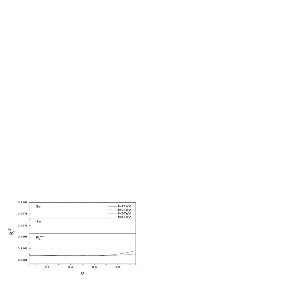
Figure 1: The branching ratio $R_{b}^{LG}$ as a function of the mixing parameter $c$ for the mixing parameter $c^{\prime}=\frac{1}{\sqrt{2}}$, $f=1TeV$, $2TeV$, $3TeV$ and $4TeV$.

Using the same method as calculating the contributions of the topcolor gauge bosons to $R_{b}$[14,15], we can give the corrections of the neutral gauge boson $Z^{\prime}$ exchange and $B^{\prime}$ exchange to the $Zq\overline{q}$ couplings $g_{L}^{q}$ and $g_{R}^{q}$:

$$\delta g_{L}^{q_{i},2} = \frac{e^{2}c^{2}}{24\pi^{2}S^{2}_{W}s^{2}}\frac{m_{Z}^{2}}{M_{Z^{\prime}}^{2}}\ln\frac{M_{Z^{\prime}}^{2}}{m_{Z}^{2}}g_{L}^{q_{i},SM},\hskip 14.22636pt\delta g_{R}^{q_{i},2}=0,$$ (20)

$$\delta g_{L}^{q_{j},2} = \frac{e^{2}c^{2}}{24\pi^{2}S^{2}_{W}s^{2}}\frac{m_{Z}^{2}}{M_{Z^{\prime}}^{2}}\ln\frac{M_{Z^{\prime}}^{2}}{m_{Z}^{2}}g_{L}^{q_{j},SM},\hskip 14.22636pt\delta g_{R}^{q_{j},2}=0,$$ (21)

$$\delta g_{L}^{q_{i},3} = \frac{e^{2}}{54\pi^{2}C^{2}_{W}s^{\prime 2}c^{\prime 2}}[\frac{1}{5}-\frac{1}{2}c^{\prime 2}]^{2}\frac{m_{Z}^{2}}{M_{B^{\prime}}^{2}}\ln\frac{M_{B^{\prime}}^{2}}{m_{Z}^{2}}g_{R}^{q_{i},SM},$$ (22)

$$\delta g_{R}^{q_{i},3} = \frac{2e^{2}}{27\pi^{2}C^{2}_{W}s^{\prime 2}c^{\prime 2}}[-\frac{1}{5}+\frac{1}{2}c^{\prime 2}]^{2}\frac{m_{Z}^{2}}{M_{B^{\prime}}^{2}}\ln\frac{M_{B^{\prime}}^{2}}{m_{Z}^{2}}g_{R}^{q_{i},SM},$$ (23)

$$\delta g_{L}^{q_{j},3} = \frac{e^{2}}{54\pi^{2}C^{2}_{W}s^{\prime 2}c^{\prime 2}}[\frac{1}{5}-\frac{1}{2}c^{\prime 2}]^{2}\frac{m_{Z}^{2}}{M_{B^{\prime}}^{2}}\ln\frac{M_{B^{\prime}}^{2}}{m_{Z}^{2}}g_{R}^{q_{j},SM},$$ (24)

$$\delta g_{R}^{q_{j},3} = \frac{8e^{2}}{27\pi^{2}C^{2}_{W}s^{\prime 2}c^{\prime 2}}[\frac{1}{5}-\frac{1}{2}c^{\prime 2}]^{2}\frac{m_{Z}^{2}}{M_{B^{\prime}}^{2}}\ln\frac{M_{B^{\prime}}^{2}}{m_{Z}^{2}}g_{R}^{q_{j},SM}.$$ (25)

Where $M_{Z^{\prime}}$ and $M_{B^{\prime}}$ are the masses of the gauge boson $Z^{\prime}$ and the heavy photon $B^{\prime}$, respectively, which have been listed in appendix A. In above equations, we have used the expressions of the $Z^{\prime}q\overline{q}$ and $B^{\prime}q\overline{q}$ couplings given in appendix B. Adding all the corrections together, we obtain the total corrections of extra gauge bosons to $R_{b}$:

$$\delta g_{L}^{b,G} = \delta g_{L}^{b,1}+\delta g_{L}^{b,2}+\delta g_{L}^{b,3},\hskip 28.45274pt\delta g_{R}^{b,G}=\delta g_{R}^{b,1}+\delta g_{R}^{b,3},$$ (26)

$$\delta g_{L}^{c,G} = \delta g_{L}^{c,1}+\delta g_{L}^{c,2}+\delta g_{L}^{c,3},\hskip 28.45274pt\delta g_{R}^{c,G}=\delta g_{R}^{c,1}+\delta g_{R}^{c,2}+\delta g_{R}^{c,3}.$$ (27)

Plugging Eqs.(15)-(27) into Eq.(13), we can obtain the relative correction $\frac{\delta R_{b}^{LG}}{R_{b}^{SM}}$ given by the new gauge bosons. In our calculation, we have taken $R_{b}^{LG}=R_{b}^{SM}+\delta R_{b}^{LG}$, $R_{b}^{SM}=0.21572$, and $R_{b}^{exp}=0.21664\pm 0.00065$[16]. Our numerical results are summarized in Fig.1 and Fig.2, in which we have used the horizontal solid line to denote the central value of $R_{b}^{exp}$ and dotted lines to show the $1\sigma$ and $2\sigma$ bounds. In Fig.1(Fig.2) we plot $R_{b}^{LG}$ as a function of the mixing parameter $c(c^{\prime})$ for $c^{\prime}=\frac{1}{\sqrt{2}}(c=\frac{1}{\sqrt{2}})$ and the scale parameter $f=1TeV$(solid line), $2TeV$(dashed line), $3TeV$(dotted line) and $4TeV$(dotted-dashed line). From Fig.1 and Fig.2, one can see that the contributions of the new gauge bosons to $R_{b}$ decrease as the scale parameter $f$ increasing. For $c^{\prime}=\frac{1}{\sqrt{2}}$, $R_{b}^{LG}$ is insensitive to the mixing parameter $c$ and the value of $\delta R_{b}^{LG}$ is very small. For $c=\frac{1}{\sqrt{2}}$, the new gauge bosons decrease the value of the branching ratio $R_{b}$ for $c^{\prime}>0.72$ and $f>1TeV$. To make the predicted $R_{b}$ value satisfy the precision experimental value in $2\sigma$ bound, we should have $0.57<c^{\prime}<0.73$ for $f=1TeV$. For $c=\frac{1}{\sqrt{2}}$, $f>2TeV$, the predicted value of $R_{b}$ is consistent with the precision experimental value $R_{b}^{exp}$ within $2\sigma$ bound in most of the allowed range of the mixing parameter $c^{\prime}$.

Figure 2: The branching ratio $R_{b}^{LG}$ as a function of the mixing parameter $c^{\prime}$ for $c=\frac{1}{\sqrt{2}}$ and $f=1TeV$, $2TeV$, $3TeV$ and $4TeV$.

From above discussions, we can see that the corrections of new gauge bosons to $R_{b}$ can be divided into two parts: one part is the tree-level corrections coming from the shift in the $Z$ couplings to quarks and the modifications of the relations between the SM parameters and the precision electroweak input parameters and the second part is the one-loop corrections coming from the neutral gauge bosons $Z^{\prime}$ exchange and $B^{\prime}$ exchange. To compare the tree-level corrections with the one-loop corrections, we plot $R=|\delta R_{b}^{1-loop}/\delta R_{b}^{tree-level}|$ as a function of the mixing parameter $c^{\prime}$ for $f=2TeV$ and $c=\frac{1}{\sqrt{2}}$ in Fig.3. One can see from Fig.3 that the one-loop contribution is smaller than the tree-level contribution at least by two orders of magnitude in all of the parameter space.

Figure 3: The relative correction $R$ as a function of the mixing parameter $c^{\prime}$ for $f=2TeV$ and $c=\frac{1}{\sqrt{2}}$.

IV. The corrections of the top quark $t$ and vector-like quark $T$ to $R_{b}$

It is well known that $R_{b}$ is almost independent of the EW oblique and QCD corrections. However, for $Zb\overline{b}$ couplings, there is an important correction coming from the top triangle diagrams, which can not be ignored. They can generate significant $m_{t}-$enhanced contributions to $R_{b}$[17]. Furthermore, the extra top quark predicted by NP can also produce significant corrections to $R_{b}$ at one-loop[1,18]. In this section, we will calculate the corrections of the top quark $t$ and vector-like quark $T$ to $R_{b}$ via the couplings $W\overline{t}b$, $W\overline{T}b$, $W^{\prime}\overline{t}b$ and $W\overline{T}b$. The relevant Feynman diagrams are shown in Fig.4.

Since the gauge bosons $W$ and $W^{\prime}$ can only couple to the left handed quark $s,t,T$ and $b$, the top and vector-like top triangle loops have no contributions to the right-handed $Zb\overline{b}$ coupling $g_{R}^{b}$. If we assume that the mass of the bottom quark is approximately equal to zero, then the corrections to the $Zb\overline{b}$ coupling $g_{L}^{b}$ generated by the $W\overline{t}b$ and $W^{\prime}\overline{t}b$ couplings can be written as:

$$\delta g_{Lt}^{b,1}=(\frac{e}{S_{W}C_{W}})\{-\frac{\alpha}{4\pi S_{W}^{2}}[F_{1}(x_{t})+\frac{c^{2}}{s^{2}}F_{1}(x^{\prime}_{t})]+\frac{3\alpha C_{W}^{2}}{8\pi S^{2}_{W}}[F_{2}(x_{t})+\frac{c^{2}}{s^{2}}F_{2}(x^{\prime}_{t})]\}$$ (28)

with

$$F_{1}(x) = \frac{g_{L}^{t}}{2}[\frac{x(x-2)}{(x-1)^{2}}\ln x+\frac{x}{x-1}]+g_{R}^{t}[\frac{x}{(x-1)^{2}}\ln x-\frac{x}{x-1}],$$ (29)

$$F_{2}(x) = \frac{x^{2}}{(x-1)^{2}}\ln x-\frac{x}{x-1},$$ (30)

where $x_{t}=(\frac{m_{t}}{m_{W}})^{2}$ and $x^{\prime}_{t}=(\frac{m_{t}}{M_{W^{\prime}}})^{2}$. In above equation, we have neglected the interference effects between gauge bosons $W^{\prime}$ and $W$.

Figure 4: Feynman diagrams for the contributions of the top quark $t$ and vector-like quark $T$ to the $Zb\overline{b}$ vertex .

In the LH model, due to the mixing between the top quark $t$ and the vector like quark $T$, the tree-level $Zt\overline{t}$ couplings receive corrections at the order of $\frac{\nu^{2}}{f^{2}}$, which also have contributions to the $Zb\overline{b}$ coupling $g_{L}^{b}$:

$$\delta g_{Lt}^{b,2}=-(\frac{e}{S_{W}C_{W}})\frac{\alpha}{16\pi S_{W}^{2}}(\frac{\nu^{2}x_{L}^{2}}{f^{2}})[x_{t}(2-\frac{4}{x_{t}-1}\log x_{t})+\frac{c^{2}}{s^{2}}x^{\prime}_{t}(2-\frac{4}{x^{\prime}_{t}-1}\log x^{\prime}_{t})].$$ (31)

The mixing angle parameter between the SM top quark $t$ and the vector-like quark $T$ is defined as $x_{L}=\frac{\lambda_{1}^{2}}{\lambda_{1}^{2}+\lambda_{2}^{2}}$, in which $\lambda_{1}$ and $\lambda_{2}$ are the coupling parameters.

Figure 5: The branching ratio $R_{b}^{LT}$ as a function of the mixing parameter $c$ for $f=2TeV$ and three values of the scale parameter $x_{L}$.

The contributions of the vector like top quark $T$ to $R_{b}$ via the couplings $W\overline{T}b$ and $W^{\prime}\overline{T}b$ can be written as:

$$\delta g_{Lt}^{b,3}=(\frac{e}{S_{W}C_{W}})\frac{\nu^{2}x_{L}^{2}}{f^{2}}\{-\frac{\alpha}{4\pi S_{W}^{2}}[F_{3}(x_{T})+\frac{c^{2}}{s^{2}}F_{3}(x^{\prime}_{T})]+\frac{3\alpha C_{W}^{2}}{8\pi S^{2}_{W}}[F_{2}(x_{T})+\frac{c^{2}}{s^{2}}F_{2}(x^{\prime}_{T})]\}$$ (32)

with

$$F_{3}(x)=\frac{g_{L}^{T}}{2}[\frac{x(x-2)}{(x-1)^{2}}\ln x+\frac{x}{x-1}]+g_{R}^{T}[\frac{x}{(x-1)^{2}}\ln x-\frac{x}{x-1}],$$ (33)

where $x_{T}=(\frac{M_{T}}{m_{W}})^{2}$ and $x^{\prime}_{T}=(\frac{M_{T}}{M_{W^{\prime}}})^{2}$. The $t-T$ contributions can be given by

$$\delta g_{Lt}^{b,4} = (\frac{e}{S_{W}C_{W}})\frac{\alpha}{4\pi S_{W}^{2}}(\frac{\nu x_{L}}{f})[\frac{1}{x_{T}-x_{t}}(\frac{x_{T}^{2}}{x_{T}-1}\log x_{T}-\frac{x_{t}^{2}}{x_{t}-1}\log x_{t})$$ (34)

$$-\frac{x_{t}x_{T}}{x_{T}-x_{t}}(\frac{x_{T}}{x_{T}-1}\log x_{T}-\frac{x_{t}}{x_{t}-1}\log x_{t})].$$

Being CKM suppression, the contributions of the top quark $t$ and vector-like quark $T$ to the couplings of the gauge boson $Z$ to other quarks($u,c,d,s$) are very small, which can be ignored. Then Eq.(13) should be changed as, for calculating the contributions of the quarks $t$ and $T$:

$$\delta R_{b}=2R_{b}^{SM}\{\frac{g_{L}^{b}\delta g_{L}^{b}+g_{R}^{b}\delta g_{R}^{b}}{(g_{L}^{b})^{2}+(g_{R}^{b})^{2}}-\frac{g_{L}^{b}\delta g_{L}^{b}+g_{R}^{b}\delta g_{R}^{b}}{2[(g_{L}^{c})^{2}+(g_{R}^{c})^{2}]+3[(g_{L}^{b})^{2}+(g_{R}^{b})^{2}]}\}.$$ (35)

Figure 6: The branching ratio $R_{b}^{LT}$ as a function of the mixing parameter $x_{L}$ for $c=\frac{1}{\sqrt{2}}$ and four values of the scale parameter $f$.

In Fig.5 we plot the branching ratio $R_{b}^{LT}=R_{b}^{SM}+\delta R_{b}^{t}+\delta R_{b}^{T}$ as a function of the mixing parameter $c$ for $f=2TeV$ and three values of the mixing parameter $x_{L}$. One can see from Fig.5 that the corrections of the top quark $t$ and vector-like quark $T$ to $R_{b}$ are not sensitive to the value of the flavor mixing parameter $c$, while are strongly dependent on the mixing parameter $x_{L}$. This is because the mass $M_{W^{\prime}}$ of the heavy gauge boson $W^{\prime}$ suppresses the contributions of the $t$ and $T$ quarks to $R_{b}$. To see the effects of $x_{L}$ varying on $R_{b}$, we plot $R_{b}^{LT}$ as a function of $x_{L}$ for $c=\frac{1}{\sqrt{2}}$, and four values of the scale parameter $f$ in Fig.6. One can see from Fig.6 that the top quark $t$ and vector-like quark $T$ can generate negative corrections to $R_{b}$ for $f\geq 1TeV$ and $x_{L}\leq 0.25$, while they can give positive corrections to $R_{b}$ for $f\leq 4TeV$ and $x_{L}\geq 0.66$.

V. The contributions of scalars to the branching ratio $R_{b}$

Figure 7: Feynman diagrams for the contributions of the charged scalars $\Phi^{\pm}$ to the $Zb\overline{b}$ vertex via the couplings $\Phi\overline{t}b$ and $\Phi\overline{T}b$.

Since the doubly charged scalars can not couple to the SM fermions, so they have no contributions to $R_{b}$. The singly charged scalars $\Phi^{\pm}$ can give contributions to the branching ratio $R_{b}$ via the couplings $\Phi\overline{t}b$ and $\Phi\overline{T}b$. The relevant Feynman diagrams for the corrections of the charged scalars $\Phi^{\pm}$ to the $Zb\overline{b}$ couplings $g_{L}^{b}$ and $g_{R}^{b}$ are shown in Fig.7.

Using the Feynman rules given in appendix C and other Feynman rules, we can give:

$$\delta g_{R}^{b,s} = 0,$$

$$\delta g_{L}^{b,s} = \frac{e}{S_{W}C_{W}}\frac{m_{t}^{2}}{32\pi^{2}\nu^{2}}(\frac{\nu}{f}-4\frac{\nu^{\prime}}{\nu})[A_{t}+\frac{x_{L}}{1-x_{L}}A_{T}],$$ (36)

with

$$A_{q} = -g_{L}^{b,SM}\overline{B_{1}}(-P_{b},m_{q},M_{\Phi})+g_{R}^{t,SM}[2\overline{C}_{24}^{\ast}(P_{b},-k,M_{\Phi},m_{q},m_{q})+\overline{B_{0}}(-k,m_{f},m_{q})$$ (37)

$$\hskip 28.45274pt-M^{2}_{\Phi}C_{0}^{\ast}(P_{b},-k,M_{\Phi},m_{q},m_{q})]+m^{2}_{t}g_{L}^{t,SM}C_{0}^{\ast}(P_{b},-k,M_{\Phi},m_{q},m_{q})$$

$$\hskip 28.45274pt+s_{W}^{2}\overline{C}_{24}(-P_{b},k,m_{q},M_{\Phi},M_{\Phi}),$$

where $q$ represents the SM top quark $t$ or the vector-like quark $T$. $B_{i}$, $C_{i}$ and $C_{ij}$ are the standard Feynman integrals[19], in which the variable $P_{b}$ is the momentum of $b$ quark, $k$ is the momentum of the gauge boson $Z$.

Figure 8: The branching ratio $R_{b}^{LS}$ as a function of the scale parameter $f$ for three values of the mixing parameter $x_{L}$.

Certainly, the neutral scalars $H^{0}$ and $\Phi^{0}$ can also generate corrections to the $Zb\overline{b}$ couplings $g_{L}^{b}$ and $g_{R}^{b}$ via the couplings $H^{0}b\overline{b}$ and $\Phi^{0}b\overline{b}$. However, compared with the charged scalar contributions, the neutral scalar contributions are suppressed at least by the factor $\frac{m_{b}^{2}}{m_{t}^{2}}$ and thus can be ignored. In order to get a positive definite mass $M_{\Phi}$ of the triplet scalars, we should have that the value of the ratio of the scalar triplet VEV $\nu^{\prime}$ to the scalar doublet VEV $\nu$ is smaller than $\frac{\nu}{4f}$. To simply our calculation, we assume $\frac{\nu^{\prime}}{\nu}=\frac{1}{5}\frac{\nu}{f}$. In this case, the triplet scalar mass $M_{\Phi}$ given in appendix A can be written as: $M_{\Phi}=10m^{2}_{H}f^{2}/\nu^{2}$, which $m_{H}$ is the SM Higg mass.

Figure 9: The branching ratio $R_{b}^{LS}$ as a function of $\frac{\nu^{\prime}}{\nu}$ for $f=3TeV$ and $x_{L}=0.2,0.5$ and $0.8$.

In Fig.8 we plot the branching ratio $R_{b}^{LS}=R_{b}^{SM}+\delta R_{b}^{LS}$ as a function of the scale parameter $f$ for $x_{L}=0.2$(solid line), $0.5$(dashed line), and $0.8$(dotted line), in which we have taken the SM Higgs mass $m_{H}=120GeV$. We can see from Fig.8 that the charged scalars $\Phi^{\pm}$ generate the negative corrections to the branching ratio $R_{b}$. The negative corrections increase as the scale parameter $f$ decreasing and the mixing parameter $x_{L}$ increasing. For the parameter $f\rightarrow\infty$, the corrections of the charged scalars to $R_{b}$ go to zero. However, the varying value of $R_{b}$ is very small and is smaller than that generated by the new gauge bosons, the top quark $t$ and vector-like quark $T$ in most of the parameter space.

To see the effects of varying the triplet scalar VEV $\nu^{\prime}$ on the branching ratio $R_{b}$, we take $f=3TeV$, which means $\frac{\nu^{\prime}}{\nu}<\frac{\nu}{4f}=0.0205$. The $R_{b}^{LS}$ is plotted in Fig.9 as a function of $\frac{\nu^{\prime}}{\nu}$ for $f=3TeV$ and three values of the mixing parameter $x_{L}$. From Fig.9 we can see that the contributions of the charged scalars to $R_{b}$ decrease as the value of the ratio $\frac{\nu^{\prime}}{\nu}$ increasing for the fixed value of the parameter $f$ and $\frac{\nu^{\prime}}{\nu}<\frac{\nu}{4f}$. If we assume that the value of the ratio $\frac{\nu^{\prime}}{\nu}$ goes to $\frac{\nu}{4f}$, then the correction value goes to zero.

VI. Discussions and conclusions

The LH model predicts the existence of several scalars, new gauge bosons, and vector-like quark $T$. These new particles can generate corrections to the branching ratio $R_{b}$. Thus, the predicted value of $R_{b}$ can be written as $R_{b}^{LH}=R_{b}^{SM}+\delta R_{b}^{LG}+\delta R_{b}^{LT}+\delta R_{b}^{LS}$ in the LH model. So, using the experimental value $R_{b}^{exp}$, we might give the constraints on the free parameters of the LH model.

Figure 10: The predicted value of $R_{b}^{LH}$ in the LH model as a function of the mixing parameter $c^{\prime}$ for four values of the scale parameter $f$.

From above discussions one can see that the correction effects of the new particles predicted by the LH model to the branching ratio $R_{b}$ decrease as the scale parameter $f$ increasing. The charged scalars generate the negative correction to $R_{b}$ in all of the parameter space. The correction value increases as the mixing parameter $x_{L}$ increasing, which is very small. The contributions of the top quark $t$ and the vector-like $T$ are related to the parameters $c$ and $x_{L}$. However, they are insensitive to the parameter $c$, while are strongly dependent on the parameters $x_{L}$ and $f$. The new gauge bosons, such as $Z^{\prime}$ and $B^{\prime}$, can give corrections to $R_{b}$ at tree-level and one-loop. The one-loop contributions are smaller than the tree-level contributions at least by two orders of magnitude in most of the parameter space. These contributions are sensitive to the parameters $c^{\prime}$ and $f$. Thus, the total correction of the LH model to the branching ratio $R_{b}$ is mainly dependent on the parameters $f$, $c^{\prime}$ and $x_{L}$. Thus, we can take the parameters $c$ and $\frac{\nu^{\prime}}{\nu}$ as fixed value: $c=\frac{1}{\sqrt{2}}$ and $\frac{\nu^{\prime}}{\nu}=\frac{\nu}{5f}$ for calculating the total correction to $R_{b}$.

Figure 11: The predicted value of $R_{b}^{LH}$ in the LH model as a function of the mixing parameter $x_{L}$ for four values of the mixing parameter $c^{\prime}$.

In Fig.10 we plot the branching ratio $R_{b}^{LH}$ as a function of the mixing parameter $c^{\prime}$ for $x_{L}=0.5$ and four values of the scale parameter $f$. From Fig.10 we can see that the value of $R_{b}^{LH}$ decreases as the parameter $c^{\prime}$ increasing. For $f=1TeV$, the value of $R_{b}$ is too large to consistent with the precision experimental value $R_{b}^{exp}$ in most of the parameter space. Furthermore, the large value of the scale parameter $f$ is in favor of the general expectation based on other phenomenological explorations. Thus, in Fig.11, we take $f=3TeV$ and plot the $R_{b}^{LH}$ as a function of the mixing parameter $x_{L}$ for four values of the parameter $c^{\prime}$. From Fig.11 we can see that the value of $R^{LH}_{b}$ decreases as the parameter $x_{L}$ increasing. If we demand that the predicted value $R^{LH}_{b}$ consistent with the precision experimental value $R^{exp}_{b}$ within $2\sigma$ bound for $f=3TeV$, there must be:

$$c^{\prime}=0.1,\hskip 28.45274pt0.16\leq x_{L}\leq 0.67;\hskip 28.45274ptc^{\prime}=0.4,\hskip 28.45274pt0.25\leq x_{L}\leq 0.74;$$

$$c^{\prime}=\frac{1}{\sqrt{2}},\hskip 28.45274pt0.38\leq x_{L}\leq 0.84;\hskip 28.45274ptc^{\prime}=0.9,\hskip 28.45274pt0.39\leq x_{L}\leq 0.83.$$

If we take the small value for the scale parameter f, these constraints will became more strong. For example, for $f=2TeV$ and $c^{\prime}=c=\frac{1}{\sqrt{2}}$, we have $0.28\leq x_{L}\leq 0.65$ in order to $R_{b}^{LH}$ consistent with $R_{b}^{exp}$ within $2\sigma$ bound.

Little Higgs models have generated much interest as possible alternatives to weak scale supersymmetry. The LH model is a minimal model of this type, which realizes the little Higgs idea. In this paper, we study the corrections of the new particles predicted by the LH model to the branching ratio $R_{b}$. We find that the corrections of the neutral scalars to $R_{b}$ is very small, which can be neglected. The charged scalars can generated the negative corrections to $R_{b}$. The new gauge bosons and fermions might generate the positive or negative corrections to $R_{b}$, which dependent on the values of the mixing parameters $c$, $c^{\prime}$ and $x_{L}$. If we demand that the contributions of the new gauge bosons and fermions cancel those generated by the charged scalars and make the predicted value $R_{b}^{LH}$ consistent with the precision experimental value $R_{b}^{exp}$, then the parameters $x_{L}$, $c^{\prime}$ and $f$ must be severe constrained.

Acknowledgments

This work was supported in part by the National Natural Science Foundation of China (90203005).

Appendix A: The masses of the gauge bosons $Z^{\prime}$ and $B^{\prime}$, triplet scalar $\Phi$, and the vector-like quark $T$.

The masses of the gauge bosons $Z^{\prime}$, $B^{\prime}$ and $W^{\prime}$ can be written at the order of $\frac{\nu^{2}}{f^{2}}$:

$$M_{Z^{\prime}}^{2} = m_{Z}^{2}C_{W}^{2}[\frac{f^{2}}{s^{2}c^{2}\nu^{2}}-1-\frac{5S_{W}^{3}}{2C_{W}}\cdot\frac{sc(c^{2}s^{\prime 2}+s^{2}c^{\prime 2})}{s^{\prime}c^{\prime}(5C_{W}^{2}s^{\prime 2}c^{\prime 2}-S_{W}^{2}s^{2}c^{2})}],$$ (38)

$$M_{B^{\prime}}^{2} = m_{Z}^{2}S_{W}^{2}[\frac{f^{2}}{5s^{\prime 2}c^{\prime 2}\nu^{2}}-1+\frac{5C_{W}^{3}}{8S_{W}}\cdot\frac{s^{\prime}c^{\prime}(c^{2}s^{\prime 2}+s^{2}c^{\prime 2})}{sc(5C_{W}^{2}s^{\prime 2}c^{\prime 2}-S_{W}^{2}s^{2}c^{2})}],$$ (39)

$$M_{W^{\prime}}^{2} = m_{Z}^{2}c_{W}^{2}(\frac{f^{2}}{s^{2}c^{2}\nu^{2}}-1),$$ (40)

where $m_{Z}$ is the mass of the SM gauge boson $Z$, $\nu$ is the electroweak scale.

For the triplet scalar $\Phi$, we have

$$M_{\Phi}^{2}=2m_{H}^{2}\frac{f^{2}}{\nu^{2}}\frac{1}{1-(\frac{4f}{\nu}\frac{\nu^{\prime}}{\nu})^{2}},$$

where $m_{H}$ is the SM Higgs mass and $\nu^{{}^{\prime}}$ is the triplet scalar vacuum expectation value(VEV).

The mass of the heavy vector-like quark $T$ can be written as:

$$M_{T}=\frac{m_{t}f}{\nu}\sqrt{\frac{1}{x_{L}(1-x_{L})}}[1-\frac{\nu^{2}}{2f^{2}}x_{L}(1+x_{L})],$$ (41)

where $m_{t}$ is the SM top quark mass, $x_{L}$ is the mixing parameter between the SM top quark and the heavy vector-like quark $T$, which is defined as $x_{L}=\frac{\lambda_{1}^{2}}{\lambda^{2}_{1}+\lambda^{2}_{2}}$. $\lambda_{1}$ and $\lambda_{2}$ are the Yukawa coupling parameters.

Appendix B: The relevant coupling constants of the gauge bosons to fermions.

$$W\overline{t}b:g_{L}^{\overline{t}b} = \frac{ie}{\sqrt{2}S_{W}}[1-\frac{\nu^{2}}{2f^{2}}(x_{L}^{2}+c^{2}(c^{2}-s^{2}))]V_{tb}^{SM},$$ (42)

$$g_{R}^{\overline{t}b} = 0,$$ (43)

where $V_{tb}^{SM}$ is the SM CKM matrix element. In our calculation, we will take $V_{tb}^{SM}=1$.

$$W\overline{T}b: g_{L}^{\overline{T}b}=\frac{e}{\sqrt{2}S_{W}}\frac{\nu}{f}x_{L}V_{tb}^{SM},\hskip 28.45274ptg_{R}^{\overline{T}b}=0.$$ (44)

$$W^{\prime}\overline{t}b: g_{L}^{\overline{t}b}=-\frac{e}{\sqrt{2}S_{W}}\frac{c}{s}V_{tb}^{SM},\hskip 28.45274ptg_{R}^{\overline{t}b}=0.$$ (45)

$$W^{\prime}\overline{T}b: g_{L}^{\overline{t}b}=-\frac{e}{\sqrt{2}S_{W}}\frac{\nu}{f}x_{L}\frac{c}{s}V_{tb}^{SM},\hskip 28.45274ptg_{R}^{\overline{t}b}=0.$$ (46)

$$Zb\overline{b}: g_{L}^{b}=\frac{e}{S_{W}C_{W}}\{-\frac{1}{2}+\frac{1}{3}S_{W}^{2}+\frac{\nu^{2}}{f^{2}}[\frac{c^{2}(c^{2}-s^{2})}{4}$$

$$\hskip 42.67912pt+\frac{5}{6}(c^{\prime 2}-s^{\prime 2})(\frac{1}{5}-\frac{1}{2}c^{\prime 2})]\},$$

$$g_{R}^{b}=\frac{e}{S_{W}C_{W}}[\frac{1}{3}S_{W}^{2}+\frac{5}{3}\frac{\nu^{2}}{f^{2}}(c^{\prime 2}-s^{\prime 2})(\frac{1}{5}-\frac{1}{2}c^{\prime 2})].$$

$$Zt\overline{t}: g_{L}^{t}=\frac{e}{S_{W}C_{W}}\{1-\frac{2}{3}S_{W}^{2}-\frac{\nu^{2}}{f^{2}}[x_{L}^{2}+\frac{c^{2}(c^{2}-s^{2})}{4}$$

$$\hskip 42.67912pt+\frac{5}{2}(c^{\prime 2}-s^{\prime 2})(\frac{4}{5}-c^{\prime 2}+\frac{2}{3}s^{\prime 2}x_{L})]\},$$

$$g_{R}^{t}=\frac{e}{S_{W}C_{W}}\{-\frac{2}{3}S_{W}^{2}-\frac{\nu^{2}}{f^{2}}5(c^{\prime 2}-s^{\prime 2})[\frac{3}{5}-c^{\prime 2}(1-\frac{1}{3}x_{L}+\frac{2}{15}x_{L})]\}.$$

$$ZT\overline{T}: g_{L}^{T}\approx g_{R}^{T}=\frac{e}{S_{W}C_{W}}(-\frac{2}{3}S_{W}^{2}),$$ (49)

$$Zt\overline{T}: g_{L}^{tT}=-i\frac{e}{S_{W}C_{W}}\frac{x_{L}\nu}{4f},\hskip 28.45274ptg_{R}^{tT}=0.$$ (50)

$$ZW^{+}W^{-}: g^{ZWW}=g^{ZW^{\prime}W^{\prime}}=-\frac{eC_{W}}{S_{W}}$$ (51)

$$Z^{\prime}b\overline{b}: g_{L}^{b}=-\frac{e}{2S_{W}}\cdot\frac{c}{s},\hskip 28.45274ptg_{R}^{b}=0$$ (52)

$$Z^{\prime}t\overline{t}: g_{L}^{t}=\frac{e}{S_{W}}\cdot\frac{c}{2s},\hskip 28.45274ptg_{R}^{t}=0.$$ (53)

$$Z^{\prime}T\overline{T}: g_{L}^{T}=g_{R}^{T}=-\frac{e}{S_{W}C_{W}}(\frac{2}{3}S_{W}^{2}).$$ (54)

$$B^{\prime}b\overline{b}: g_{L}^{b}=\frac{e}{3C_{W}s^{\prime}c^{\prime}}(\frac{1}{5}-\frac{1}{2}c^{\prime 2}),\hskip 28.45274ptg_{R}^{b}=\frac{2e}{3C_{W}s^{\prime}c^{\prime}}(-\frac{1}{5}+\frac{1}{2}c^{\prime 2}).$$ (55)

$$B^{\prime}c\overline{c}: g_{L}^{c}=\frac{e}{3C_{W}s^{\prime}c^{\prime}}(\frac{1}{5}-\frac{1}{2}c^{\prime 2}),\hskip 28.45274ptg_{R}^{c}=\frac{4e}{3C_{W}s^{\prime}c^{\prime}}(\frac{1}{5}-\frac{1}{2}c^{\prime 2}).$$ (56)

Appendix C: The coupling constants of the scalars to fermions.

$$H^{0}b\overline{b}: -i\frac{m_{b}}{\nu}(1-4\frac{\nu^{\prime 2}}{\nu^{2}}+2\frac{\nu^{\prime}}{f}-\frac{2}{3}\frac{\nu^{2}}{f^{2}}).$$ (57)

$$\Phi^{0}b\overline{b}: -i\frac{m_{b}}{\sqrt{2}\nu}(\frac{\nu}{f}-4\frac{\nu^{\prime}}{\nu}).$$ (58)

$$\Phi^{P}b\overline{b}: \frac{m_{b}}{\sqrt{2}\nu}(\frac{\nu}{f}-4\frac{\nu^{\prime}}{\nu}).$$ (59)

$$\Phi^{+}\overline{t}b: -\frac{i}{\sqrt{2}\nu}[m_{t}P_{L}+m_{b}P_{R}](\frac{\nu}{f}-4\frac{\nu^{\prime}}{\nu}),$$ (60)

with $P_{L}=\frac{1-\gamma_{5}}{2}$,         $P_{R}=\frac{1+\gamma_{5}}{2}$.

$$\Phi^{+}\overline{T}b:\hskip 14.22636pt-i\frac{m_{t}}{\sqrt{2}\nu}(\frac{\nu}{f}-4\frac{\nu^{\prime}}{\nu})\sqrt{\frac{x_{L}}{1-x_{L}}}P_{L}.$$ (61)

The coupling vertex of the SM gauge boson $Z$ to the charged scalars $\Phi^{\pm}$ is

$$i\frac{e}{S_{W}C_{W}}S_{W}^{2}(P_{1}-P_{2})_{\mu}.$$

References

[1]
D. Comelli and J. P. Silva, Phys. Rev. D54(1996)1176; V. D. Barger, K. M. Cheung, P. Langaclar,
Phys. Lett. B381(1996)226; P. Bamert, C. P.
Burgess, J. M. Cline, D. London, and E. Nardi, Phys. Rev. D54(1996)4275; D. Atwood, L. Reina, and A. Soni, Phys. Rev. D54(1996)3296.
[2]
N. Arkani-Hamed, A. G. Cohen, E. Katz, A. E.
Nelson, hep-ph/0206021.
[3]
N. Arkani-Hamed, A. G. Cohen and H. Georgi,
Phys. Lett. B513(2001)232; N. Arkani-Hamed, A. G. Cohen,
T. Gregoire and J. G. Wacker,
hep-ph/0202089; N. Arkani-Hamed, A. G. Cohen,
E. Katz, A. E. Nelson, T. Gregoire and J. G. Wacker,
hep-ph/0206020; I. Low, W. Skiba and
D. Smith, Phys. Rev. D66(2002)072001; M.
Schmaltz, Nucl. Phys. Proc. Suppl.117(2003)40; D. E. Kaplan and M. Schmaltz,
hep-ph/0302049.
[4]
J. G. Wacker, hep-ph/0208235; S. Chang and J. G. Wacker,
hep-ph/0303001;
W. Skiba and J. Terning, Phys. Rev. D68(2003)075001; S.
Chang, hep-ph/0306034.
[5]
T. Han, H. E. Logan, B. McElrath and L. T. Wang,
Phys. Rev. D67(2003)095004.
[6]
M. Perelstein, M. E. Peskin and A. Pierce, hep-ph / 0310039.
[7]
G. Burdman. M. Perelstein and A. Pierce,
Phys. Rev. Lett.90(2003)241802;
C. Dib, R. Rosenfeld and A. Zerwekh, hep-ph/0302068;
T. Han, H. E. Logan, B. McElrath ans L. T. Wang,
Phys. Lett. B563(2003)191; Z. Sullivan,
hep-ph/0306266; S. C. Park and J. Song, hep-ph/0306112;
Chongxing Yue, Shunzhi Wang, Dongqi Yu,
hep-ph/0309113.
[8]
C. Csaki, J. Hubisz, G. D. Kribs, P. Meade and J.
Terning, Phys. Rev. D67(2003)115002;
D68(2003)035009; T. L. Hewett, F. J.
Petrielo and J. G. Rizzo, hep-ph/0211218; T. Gregoire,
D. R. Smith and J. G. Wacker, hep-ph/0305275;
Wujun Huo and Shouhua Zhu, Phys. Rev. D68(2003)097301;;
N. Mahajan, hep-ph/0310098.
[9]
Mu-Chun Chen and S. Dawson, hep-ph/0311032; R.
Casalbuoni, A. Deandrea, M. Oertel, hep-ph/0311038; W. Kilian and J. Reuter, hep-ph/0311095; S. Chang and Hong-Jian He, hep-ph/0311177; C. Kilic and R. Mahbubani, hep-ph/0312053.
[10]
S. R. Coleman and F. Weinberg, Phys. Rev.D7(1973)1888.
[11]
For review see V. A. Novikov, L. B. Okun, A. N. Rozanov, and M. I.
Vysotsky, Rept. Prog. Phys.62(1999)1275.
[12]
J. Bernabeu, A. Pich, A. Santamaria, Nucl. Phys. B363(1991)326; A. Denner, R. J. Guth, W. Hollik and J. H.
Kuhn, Z. Phys. C51(1991)695; A. K. Grant, Phys. Rev. D51(1995)207.
[13]
D. E. Groom, et al. [Particle Data Group], Eur. Phys. J.
C15(2000)1; K. Hagiwora et al. [Particle Data
Group], Phys. Rev. D66(2002)010001.
[14]
C. T. Hill and X. Zhang, Phys. Rev. D51(1995)3563; C. X. Yue, Y. P. Kuang, X. L. Wang, and W.
B. Li, Phys. Rev. D62(2000)055005.
[15]
C. X. Yue, Y. P. Kuang, G. R. Lu and L. D. Wan, Phys. Rev. D52(1995)5314; C. X. Yue, Y. B. Dai and H. Li, Mod. Phys. Lett. A17(2002)261.
[16]
P. Langacker, hep-ph/0308145; P. Gambino, hep-ph/0311257.
[17]
J. Bernabeu, A. Pich and A. Santamaria, Phys. Lett. B200(1988)569.
[18]
J. A. Aguilar-Saavedra, Phys. Rev. D67(2003)035003.
[19]
G. Passarino and M. Veltman, Nucl. Phys. B160(1979)151; A. Axelrod, Nucl. Phys. B209(1982)349; M. Clements etal., Phys. Rev. D27(1983)570.