SISSA 7/2004/EP
hep-ph/0401206

On Deviations from Bimaximal Neutrino Mixing

Abstract

The PMNS neutrino mixing matrix $U_{\rm PMNS}$ is in general a product of two unitary matrices $U_{\rm lep}$ and $U_{\nu}$ arising from the diagonalization of the charged lepton and neutrino mass matrices, $U_{\rm PMNS}=U^{\dagger}_{\rm lep}U_{\nu}$. Assuming that $U_{\nu}$ is a bimaximal mixing matrix, we investigate the possible forms of $U_{\rm lep}$. We identify three possible generic structures of $U_{\rm lep}$, which are compatible with the existing data on neutrino mixing. One corresponds to a hierarchical “CKM–like” matrix. In this case relatively large values of the solar neutrino mixing angle $\theta_{\rm sol}$, and of $|U_{e3}|^{2}\equiv|(U_{\rm PMNS})_{e3}|^{2}$, are typically predicted, $\tan^{2}\theta_{\rm sol}\mathrel{\hbox to0.0pt{\raise 2.20013pt\hbox{$>$}\hss}{\lower 2.20013pt\hbox{$\sim$}}}0.42$, $|U_{e3}|^{2}\mathrel{\hbox to0.0pt{\raise 2.20013pt\hbox{$>$}\hss}{\lower 2.20013pt\hbox{$\sim$}}}0.02$, while the atmospheric neutrino mixing angle $\theta_{\rm atm}$ can deviate noticeably from $\pi/4$, $\sin^{2}2\theta_{\rm atm}\mathrel{\hbox to0.0pt{\raise 2.20013pt\hbox{$>$}\hss}{\lower 2.20013pt\hbox{$\sim$}}}0.95$. The second corresponds to one of the mixing angles in $U_{\rm lep}$ being equal to $\pi/2$, and predicts practically maximal atmospheric neutrino mixing $\sin^{2}2\theta_{\rm atm}\simeq 1$. Large atmospheric neutrino mixing, $\sin^{2}2\theta_{\rm atm}\mathrel{\hbox to0.0pt{\raise 2.20013pt\hbox{$>$}\hss}{\lower 2.20013pt\hbox{$\sim$}}}0.95$, is naturally predicted by the third possible generic structure of $U_{\rm lep}$, which corresponds to all three mixing angles in $U_{\rm lep}$ being large. We focus especially on the case of CP–nonconservation, analyzing it in detail. We show how the CP–violating phases, arising from the diagonalization of the neutrino and charged lepton mass matrices, contribute to the measured neutrino mixing observables.

1 Introduction

After the spectacular results obtained in the experimental studies of neutrino oscillations in the last two and a half years or so (see, e.g., [1, 2] for a summary), understanding the detailed structure and the origin of neutrino masses and mixing is of prime importance. Progress in understanding the origin of the Pontecorvo–Maki–Nakagawa–Sakata (PMNS) mixing matrix in the weak charged lepton current [3] can lead to a complete solution of the fundamental problem regarding the structure of the neutrino mass spectrum, which can be with normal or inverted hierarchy, or of quasi–degenerate type. It can also help gain significant insight on, or even answer the fundamental question of, CP–violation in the lepton sector.

The fact that, according to the existing data, the atmospheric neutrino mixing angle is maximal, or close to maximal [4], $\theta_{\rm atm}\sim\pi/4$, the solar neutrino mixing angle is relatively large [5, 2], $\theta_{\odot}\sim\pi/5.4$ ($\sin^{2}\theta_{\odot}\cong 0.30$), and that the mixing angle $\theta$ limited by the CHOOZ and Palo Verde experiments [6, 7] is small, $\sin^{2}\theta<0.074$ (99.73% C.L.) [2], suggests that the PMNS neutrino mixing matrix , $U_{\rm PMNS}$, can originate from a 3$\times$3 unitary mixing matrix having a bimaximal mixing form, $U_{\rm bimax}$. In the case of CP–invariance in the lepton sector one has

$$U_{\rm bimax}=\left(\begin{array}[]{ccc}\frac{1}{\sqrt{2}}&\frac{1}{\sqrt{2}}&0\\[8.5359pt] -\frac{1}{2}&\frac{1}{2}&\frac{1}{\sqrt{2}}\\[8.5359pt] \frac{1}{2}&-\frac{1}{2}&\frac{1}{\sqrt{2}}\\[8.5359pt] \end{array}\right)~{}.$$ (1)

The assumption of exact equality $U_{\rm PMNS}=U_{\rm bimax}$ implies $\theta_{\odot}=\pi/4$, which is ruled out at more than 5 s.d. by the existing solar neutrino data [5, 2]. However, the deviation of $\theta_{\odot}$ from $\pi/4$ can be described by a relatively small mixing parameter [8]: $\lambda=\sin(\pi/4-\pi/5.4)\cong 0.20$. Thus, the neutrino mixing matrix can have the form

$$\mbox{$U_{\rm PMNS}$}=U_{\lambda}^{\dagger}\,U_{\rm bimax}~{}.$$ (2)

It is natural to suppose that $U_{\lambda}^{\dagger}$ and $U_{\rm bimax}$ in Eq. (2) arise from the diagonalization of the charged lepton and neutrino mass matrices, respectively.

The existing data show also that [2, 4] $\mbox{$\Delta m^{2}_{\odot}$}\ll|\mbox{$\Delta m^{2}_{\rm A}$}|$, where $\mbox{$\Delta m^{2}_{\odot}$}>0$ and $\Delta m^{2}_{\rm A}$ are the neutrino mass squared differences driving the solar and atmospheric neutrino oscillations. This fact and the preceding considerations suggest further that $U_{\rm bimax}$ can arise from the diagonalization of a neutrino mass term of Majorana type having a specific symmetry. In the absence of charged lepton mixing ($U_{\lambda}={\mathbbm{1}}$) this symmetry could correspond to the conservation of the non–standard lepton charge [9] $L^{\prime}=L_{e}-L_{\mu}-L_{\tau}$, where $L_{l}$, $l=e,\mu,\tau$, are the electron, muon and tauon lepton charges. The indicated symmetry cannot be exact: it has to be broken mildly by the neutrino mass term in order to ensure that $\Delta m^{2}_{\odot}\neq 0$, and by the charged lepton mass term ($U_{\lambda}\neq{\mathbbm{1}}$), and/or by the neutrino mass term, in order to guarantee that $\theta_{\odot}\neq\pi/4$.

The possibility expressed by Eq. (2) and described above has been discussed in the context of grand unified theories by many authors (see, e.g., [10, 11]). It has also been investigated phenomenologically first a long time ago (in a different context) in [9] and more recently in [12, 13, 14] (see also [15]). Assuming that Eq. (2) holds, we perform in the present article a systematic study of the possible forms of the matrix $U_{\lambda}^{\dagger}$ in Eq. (2), which are compatible with the existing data on neutrino mixing and oscillations. The case of CP–nonconservation is of primary interest and is analyzed in detail. We show, in particular, how the CP–violating phases, arising from the diagonalization of the neutrino and charged lepton mass matrices, can influence the form of $U_{\lambda}$ and can contribute in the measured CP–conserving and CP–violating observables, related to neutrino mixing. The analysis presented here can be considered as a continuation of the earlier studies quoted, e.g., in [10, 11, 12, 13, 14]. However, it overlaps little with them.

2 The Deviations from Bimaximal Mixing

We will employ in what follows the standard parametrization of the PMNS matrix:

$$\begin{array}[]{c}\mbox{$U_{\rm PMNS}$}=\left(\begin{array}[]{ccc}c_{12}c_{13}&s_{12}c_{13}&s_{13}\\[5.69046pt] -s_{12}c_{23}-c_{12}s_{23}s_{13}e^{i\delta}&c_{12}c_{23}-s_{12}s_{23}s_{13}e^{i\delta}&s_{23}c_{13}e^{i\delta}\\[5.69046pt] s_{12}s_{23}-c_{12}c_{23}s_{13}e^{i\delta}&-c_{12}s_{23}-s_{12}c_{23}s_{13}e^{i\delta}&c_{23}c_{13}e^{i\delta}\\ \end{array}\right){\rm diag}(1,e^{i\alpha},e^{i\beta})\,,\end{array}$$ (3)

where we have used the usual notations $c_{ij}=\cos\theta_{ij}$, $s_{ij}=\sin\theta_{ij}$, $\delta$ is the Dirac CP–violation phase, $\alpha$ and $\beta$ are two possible Majorana CP–violation phases [16, 17]. If we identify the two independent neutrino mass squared differences in this case, $\Delta m^{2}_{21}$ and $\Delta m^{2}_{31}$, with the neutrino mass squared differences which induce the solar and atmospheric neutrino oscillations, $\mbox{$\Delta m^{2}_{\odot}$}=\Delta m^{2}_{21}>0$, $\mbox{$\Delta m^{2}_{\rm A}$}=\Delta m^{2}_{31}$, one has: $\theta_{12}=\theta_{\rm sol}$, $\theta_{23}=\theta_{\rm atm}$, and $\theta_{13}=\theta$. The ranges of values of the three neutrino mixing angles, which are allowed at 1 s.d. (3 s.d.) by the current solar and atmospheric neutrino data and by the data from the reactor antineutrino experiments CHOOZ and KamLAND, read [2, 18]:

$$\begin{array}[]{c}0.35~{}(0.27)\leq\tan^{2}\theta_{\rm sol}\equiv\tan^{2}\theta_{12}\leq 0.52~{}(0.72)~{},\\[8.5359pt] |U_{e3}|^{2}=\sin^{2}\theta_{13}<0.029~{}(0.074)~{},\\[5.69046pt] \sin^{2}2\theta_{\rm atm}\equiv\sin^{2}2\theta_{23}\geq 0.95~{}(0.85)~{}.\end{array}$$ (4)

As is well–known, the oscillations between flavour neutrinos depend on the Dirac phase $\delta$, but are insensitive to the Majorana CP–violating phases $\alpha$ and $\beta$ [16, 19]. Information about these phases can be obtained, in principle, in neutrinoless double beta decay ($(\beta\beta)_{0\nu}$–decay) experiments [20, 21, 22].

Let us define the matrix $U_{\lambda}$ through Eq. (2), $\mbox{$U_{\rm PMNS}$}\equiv U_{\lambda}^{\dagger}\,U_{\rm bimax}$, where the matrix $U_{\rm bimax}$ is given by Eq. (1). The latter would have coincided with the PMNS matrix if the neutrino mixing were exactly bimaximal. The bimaximal neutrino mixing can be obtained, e.g., by exploiting the flavor neutrino symmetry corresponding to the conservation of the non–standard lepton charge $L^{\prime}=(L_{e}-L_{\mu}-L_{\tau})$ [9] (see also [23, 24]). The deviations of the neutrino mixing from the exact bimaximal mixing form can be described, as was shown in [8], by a real parameter $\lambda\sim 0.2$, which was introduced in the following “flexible” parametrization of three elements of $U_{\rm PMNS}$:

$$\begin{array}[]{c}U_{e2}=\sqrt{\frac{1}{2}}\,(1-\lambda)~{},~{}~{}~{}U_{e3}=A\,\lambda^{n}~{},~{}~{}~{}U_{\mu 3}=\sqrt{\frac{1}{2}}\,(1-B\,\lambda^{m})\,e^{i\delta}~{},\end{array}$$ (5)

where $A$ and $B$ are real parameters of order one. The integer numbers $m$ and $n$ can be chosen according to the improved limits on, or precise values of, $\sin^{2}\theta_{13}$ and $\sin^{2}2\theta_{23}$. The fact that solar neutrino mixing is now confirmed (at more than 5 s.d.) to be non–maximal means that $\lambda\neq 0$ and the best–fit value of $\mbox{$\tan^{2}\theta_{\rm sol}$}=0.43$ [2] corresponds to $\lambda\simeq 0.23$.

Taking the purely phenomenological parametrization (5) at face value and expressing the PMNS matrix in terms of $\lambda$, $A$ and $B$, one can solve Eq. (2) for $U_{\lambda}$ in order to obtain the physical ranges of values of the parameters involved. It was found in [8] that the structure of $U_{\lambda}$ can at leading order be the unit matrix plus corrections of order $\lambda$.

In the present article we perform a systematic study of the possible forms of $U_{\lambda}$ allowed by the current data. The neutrino mixing phenomenology can be described, for example, by $U_{\lambda}$ having a “CKM–like” structure, as has been discussed in [13, 14, 8]. Here we show, in particular, that the restriction to a hierarchical form for $U_{\lambda}$ is not necessary. Counter–intuitive forms of $U_{\lambda}$, and/or the presence of CP–violating phases, can produce naturally the observed deviation from $\pi/4$ of $\theta_{\rm sol}$ as well as the requisite smallness of $|U_{e3}|$.

3 The Case of CP Conservation

In this case $U_{\lambda}$ is an orthogonal matrix. We will use the standard parametrization (see Eq. (3)) for $U_{\lambda}$. Let us denote the angles in $U_{\lambda}$ as $\theta^{\prime}_{12}$, $\theta^{\prime}_{23}$, and $\theta^{\prime}_{13}$, and define $\sin\theta^{\prime}_{ij}\equiv\lambda_{ij}$. We shall treat $\lambda_{12}$, $\lambda_{23}$ and $\lambda_{13}$ as free parameters without assuming any hierarchy relation between them. In the case of CP–conservation under discussion one can limit the analysis to the case $0\leq\theta^{\prime}_{ij}\leq\pi$, and correspondingly to $0\leq\lambda_{ij}\leq 1$. The results for $\lambda_{ij}<0$ can be obtained formally from those derived for $\lambda_{ij}>0$ by making the change i) $\lambda_{23}\rightarrow-\lambda_{23}$, and/or ii) $\lambda_{13}\rightarrow-\lambda_{13}$ as long as one keeps $\lambda_{12}>0$. The change $\lambda_{12}\rightarrow-\lambda_{12}$ should be done simultaneously with the change $\lambda_{13}\rightarrow-\lambda_{13}$ and in this case only the “solutions” with $|\lambda_{13}|>|\lambda_{12}|$ should be considered. In the latter case both signs of $\lambda_{23}$ are possible.

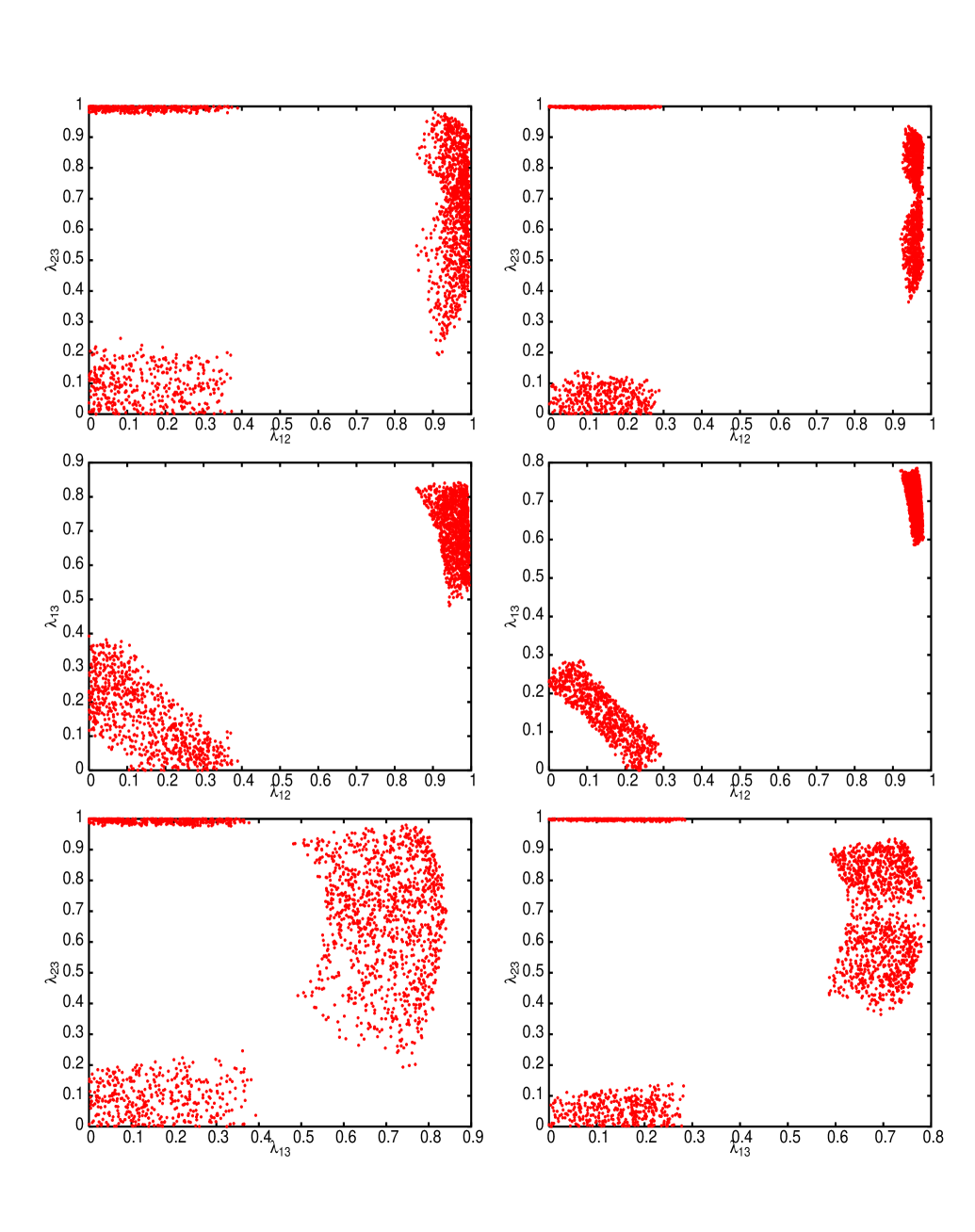
Figure 1: Scatter plot of the three $\lambda$ parameters for the 3$\sigma$ (left column) and 1$\sigma$ (right column) allowed ranges of values of the neutrino mixing parameters given in Eq. (4). Conservation of CP is assumed.

Using Eqs. (2) and (1), we have determined the regions of values of $\lambda_{12}$, $\lambda_{23}$ and $\lambda_{13}$ for which the values of the neutrino mixing angles $\theta_{12}=\theta_{\rm sol}$, $\theta_{23}=\theta_{\rm atm}$, and $\theta_{13}=\theta$, lying within their 1$\sigma$ and 3$\sigma$ ranges, Eq. (4), can be reproduced. The results are shown graphically in Fig. 1. One can clearly identify three different cases:

• all $\lambda_{ij}\mathrel{\hbox to0.0pt{\raise 2.20013pt\hbox{$<$}\hss}{\lower 2.20013pt\hbox{$\sim$}}}0.35$ (“small”),

• $\lambda_{23}=+1$ and $\lambda_{12,13}\mathrel{\hbox to0.0pt{\raise 2.20013pt\hbox{$<$}\hss}{\lower 2.20013pt\hbox{$\sim$}}}0.35$ (“small”),

• all $\lambda_{ij}\mathrel{\hbox to0.0pt{\raise 2.20013pt\hbox{$>$}\hss}{\lower 2.20013pt\hbox{$\sim$}}}0.40$ (“large”).

We shall discuss next these three cases in detail. The resulting structures of $U_{\lambda}$ will turn out to be rather different in the three cases.

3.1 Small $\lambda_{ij}$

Multiplying $\mbox{$U_{\lambda}$}\!\!^{\dagger}$ by $U_{\rm bimax}$ and expressing $\tan^{2}\theta_{\rm sol}$, $|U_{e3}|^{2}$ and $\sin^{2}2\theta_{\rm atm}$ in terms of the three small parameters $\lambda_{ij}$, one finds:

$$\begin{array}[]{c}\tan^{2}\theta_{\rm sol}=\frac{\displaystyle|U_{e1}|^{2}}{\displaystyle|U_{e2}|^{2}}\simeq 1-2\sqrt{2}\,(\lambda_{12}-\lambda_{13})+4\,(\lambda_{12}-\lambda_{13})^{2}-2\sqrt{2}\,\lambda_{23}\,(\lambda_{12}+\lambda_{13})+{\cal{O}}(\lambda^{3})~{},\\[8.5359pt] |U_{e3}|\simeq\left|\frac{\displaystyle\lambda_{12}+\lambda_{13}}{\displaystyle\sqrt{2}}-\frac{\displaystyle\lambda_{23}}{\displaystyle\sqrt{2}}\,(\lambda_{12}-\lambda_{13})+{\cal{O}}(\lambda^{3})\right|~{},\\ \sin^{2}2\theta_{\rm atm}\equiv\frac{\displaystyle 4\,|U_{\mu 3}|^{2}\,|U_{\tau 3}|^{2}}{\displaystyle(1-|U_{e3}|^{2})^{2}}\simeq 1-4\,\lambda_{23}^{2}+{\cal{O}}(\lambda^{3})~{}.\end{array}$$ (6)

The key quantities are therefore $\lambda_{23}$ and the sum and the difference of $\lambda_{12}$ and $\lambda_{13}$. To leading order in the $\lambda$–parameters, the deviation from maximal solar neutrino mixing and zero $U_{e3}$ are proportional to $\lambda$, while the atmospheric neutrino mixing is close to maximal with only quadratic corrections to $(1-\sin^{2}2\theta_{\rm atm})$. The requirement of $\sin^{2}2\theta_{\rm atm}\geq 0.85~{}(0.95)$ leads to order $\lambda^{2}$ to the restriction $\lambda_{23}\mathrel{\hbox to0.0pt{\raise 2.20013pt\hbox{$<$}\hss}{\lower 2.20013pt\hbox{$\sim$}}}0.19~{}(0.11)$.

Assuming that the oscillation parameters lie within their 1$\sigma$ allowed ranges and neglecting terms of order $\lambda^{2}$, one finds from Eq. (6) that the term $(\lambda_{12}-\lambda_{13})$ has to be positive and rather large ($\sim 0.2$) in order to ensure the deviation of $\theta_{\rm sol}$ from $\pi/4$. At the same time $(\lambda_{12}+\lambda_{13})$ has to be smaller than $\sim 0.2$ in order to satisfy the limit on $|U_{e3}|$. These two conditions imply (for $\lambda_{12,13}>0$) a hierarchy of the form $\lambda_{12}\gg\lambda_{13}$. The remaining parameter is $\lambda_{23}\mathrel{\hbox to0.0pt{\raise 2.20013pt\hbox{$<$}\hss}{\lower 2.20013pt\hbox{$\sim$}}}(\lambda_{12}+\lambda_{13})/2\sim\lambda_{12}/2$.

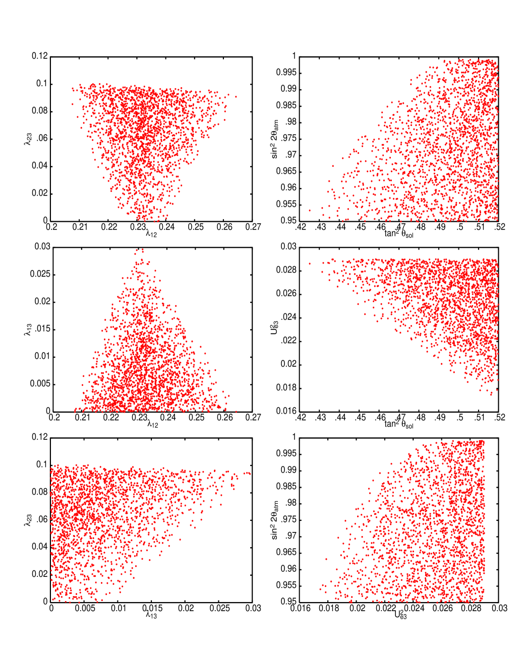
Figure 2: Scatter plot of the $\lambda$ and neutrino oscillation parameters in the case of “small” $\lambda_{ij}$ for the 1$\sigma$ allowed ranges of values of the neutrino mixing parameters given in Eq. (4). Conservation of CP is assumed.

In Fig. 2 we show scatter plots of the values of $\lambda_{ij}$, obtained by requiring that the corresponding values of neutrino mixing parameters $\tan^{2}\theta_{\rm sol}$, $\sin^{2}2\theta_{\rm atm}$ and $|U_{e3}|^{2}$ lie within their 1$\sigma$ allowed ranges, Eq. (4). One can see from the left panels in Fig. 2 that $\lambda_{12}\simeq(0.21-0.26)$, $\lambda_{23}\mathrel{\hbox to0.0pt{\raise 2.20013pt\hbox{$<$}\hss}{\lower 2.20013pt\hbox{$\sim$}}}0.10$ and $\lambda_{13}\mathrel{\hbox to0.0pt{\raise 2.20013pt\hbox{$<$}\hss}{\lower 2.20013pt\hbox{$\sim$}}}0.03$. Thus, one has $\lambda_{23}\mathrel{\hbox to0.0pt{\raise 2.20013pt\hbox{$<$}\hss}{\lower 2.20013pt\hbox{$\sim$}}}\lambda_{12}/2$ and $\lambda_{13}\mathrel{\hbox to0.0pt{\raise 2.20013pt\hbox{$<$}\hss}{\lower 2.20013pt\hbox{$\sim$}}}\lambda^{2}_{12}/2$. In Fig. 2 we also display the resulting correlations between the neutrino mixing parameters for which the 1$\sigma$ allowed ranges were used. From the panels in the right column one sees that $\mbox{$\tan^{2}\theta_{\rm sol}$}\mathrel{\hbox to0.0pt{\raise 2.20013pt\hbox{$>$}\hss}{\lower 2.20013pt\hbox{$\sim$}}}0.42$ and $|U_{e3}|^{2}\mathrel{\hbox to0.0pt{\raise 2.20013pt\hbox{$>$}\hss}{\lower 2.20013pt\hbox{$\sim$}}}0.017$. Most of the points tend to lie at rather large values of $\tan^{2}\theta_{\rm sol}$ and $|U_{e3}|^{2}$. Taking the 3$\sigma$ range in Eq. (4) leads to the lower limits of $\mbox{$\tan^{2}\theta_{\rm sol}$}\mathrel{\hbox to0.0pt{\raise 2.20013pt\hbox{$>$}\hss}{\lower 2.20013pt\hbox{$\sim$}}}0.35$ and of $|U_{e3}|^{2}\mathrel{\hbox to0.0pt{\raise 2.20013pt\hbox{$>$}\hss}{\lower 2.20013pt\hbox{$\sim$}}}0.003$.

We consider next two representative (and to a certain degree typical) forms of $U_{\lambda}$. A viable possibility is the existence of “hierarchical” relations between $\lambda_{12}$, $\lambda_{23}$ and $\lambda_{13}$. One can have, for instance, $\lambda_{23}\sim\lambda^{2}_{12}$ and $\lambda_{13}\sim\lambda^{3}_{12}$, with $\lambda_{12}\equiv\lambda$ and, e.g., $\lambda\sim(0.20-0.30)$. This implies the following form of $U_{\lambda}$:

$$\begin{array}[]{c}U_{\lambda}\sim\small\left(\begin{array}[]{ccc}1-\lambda^{2}/2&\lambda&\lambda^{3}\\[5.69046pt] -\lambda&1-\lambda^{2}/2&\lambda^{2}\\[5.69046pt] \lambda^{3}&-\lambda^{2}&1\end{array}\right)+{\cal O}(\lambda^{4})~{}.\end{array}$$ (7)

The structure of $U_{\lambda}$ is close to that of a diagonal matrix, and is similar to the structure of the CKM matrix. Given the hierarchy in the charged lepton masses, the CKM-like form of $U_{\lambda}$, Eq. (7), is rather natural. One has in this case:

$$\begin{array}[]{c}\tan^{2}\theta_{\rm sol}\simeq 1-2\sqrt{2}\,\lambda+4\,\lambda^{2}-2\sqrt{2}\,\lambda^{3}~{},\\[8.5359pt] |U_{e3}|\simeq\frac{\displaystyle\lambda}{\displaystyle\sqrt{2}}~{},\\[8.5359pt] \sin^{2}2\theta_{\rm atm}\simeq 1-4\,\lambda^{4}\end{array}$$ (8)

plus terms of higher order in $\lambda$. Consequently, this scenario “predicts” solar neutrino mixing and $|U_{e3}|^{2}$ close to their currently allowed maximal values, and atmospheric neutrino mixing close to maximal.

More specifically, the hierarchy of the $\lambda$–parameters we are considering, $\lambda_{12}\gg\lambda_{23,13}$, leads, as it follows from Eqs. (6) and (8), to the interesting correlation:

$$\tan^{2}\theta_{\rm sol}\simeq 1-4\,|U_{e3}|+8\,|U_{e3}|^{2}-8\,|U_{e3}|^{3}~{}.$$ (9)

The upper limit of $\tan^{2}\theta_{\rm sol}\leq 0.52$ (0.72) implies in this case a lower limit on $|U_{e3}|^{2}\mathrel{\hbox to0.0pt{\raise 2.20013pt\hbox{$>$}\hss}{\lower 2.20013pt\hbox{$\sim$}}}0.027~{}(0.006)$ . This explains qualitatively the lower limit on $|U_{e3}|^{2}$ as observed in Fig. 2 and mentioned earlier. Another correlation related to the CKM–like form of $U_{\lambda}$, Eq. (7), reads:

$$\sin^{2}2\theta_{\rm atm}\simeq 1-16\,|U_{e3}|^{4}~{}.$$ (10)

Thus, the deviations from maximal atmospheric neutrino mixing are determined in the case of the hierarchical relations $\lambda_{12}\equiv\lambda\gg\lambda_{23,13}$, $\lambda_{23}\sim\lambda^{2}$, by the magnitude of $|U_{e3}|^{4}$. For, e.g., $|U_{e3}|^{2}=0.029~{}(0.05)$, we have $\sin^{2}2\theta_{\rm atm}\simeq 0.975~{}(0.96)$.

The alternative possibility is that of a mild “hierarchy” between $\lambda_{12}$ and $\lambda_{23}$. We can have, for instance, $\lambda_{23}\simeq\lambda_{12}/2$, $\lambda_{12}\equiv\lambda$. Taking also $\lambda_{13}\simeq\lambda^{3}\ll\lambda_{12}$, one finds:

$$\begin{array}[]{c}\tan^{2}\theta_{\rm sol}\simeq 1-2\sqrt{2}\,\lambda+(4-\sqrt{2})\,\lambda^{2}-2\sqrt{2}\,\lambda^{3}~{},\\[8.5359pt] |U_{e3}|\simeq\frac{\displaystyle\lambda}{\displaystyle\sqrt{2}}~{},\\[8.5359pt] \sin^{2}2\theta_{\rm atm}\simeq 1-\lambda^{2}\simeq 1-2\,|U_{e3}|^{2}~{}.\end{array}$$ (11)

The atmospheric neutrino mixing angle $\theta_{\rm atm}$ can deviate more from $\pi/4$ than in the hierarchical case: for $|U_{e3}|^{2}=0.05$ we have now $\sin^{2}2\theta_{\rm atm}\simeq 0.90$. This provides a possibility to distinguish the case of $\lambda_{23}\simeq\lambda_{12}/2$, $\lambda_{12,23}\gg\lambda_{13}$, from the hierarchical one $\lambda_{13}\sim\lambda^{3}_{12}<\lambda_{23}\sim\lambda^{2}_{12}<\lambda_{12}$ considered above. For $\lambda\sim 0.24$ one finds from Eq. (11) $\tan^{2}\theta_{\rm sol}\simeq 0.43$, which is quite encouraging since values of $\lambda\sim 0.24$ could be interpreted in terms of $\sqrt{m_{\mu}/m_{\tau}}\simeq\sqrt{0.105/1.77}\simeq 0.24$.

3.2 The Case of $\lambda_{23}=1$

If $\lambda_{23}=1$ and $\lambda_{12,13}$ are “small”, $\lambda_{12,13}\mathrel{\hbox to0.0pt{\raise 2.20013pt\hbox{$<$}\hss}{\lower 2.20013pt\hbox{$\sim$}}}0.35$, we find:

$$\begin{array}[]{c}\tan^{2}\theta_{\rm sol}\simeq 1-2\sqrt{2}\,(\lambda_{12}+\lambda_{13})+4\,(\lambda_{12}+\lambda_{13})^{2}+{\cal O}(\lambda^{3})~{},\\[8.5359pt] U_{e3}\simeq\frac{\displaystyle\lambda_{12}-\lambda_{13}}{\displaystyle\sqrt{2}}+{\cal O}(\lambda^{3})~{},\\[8.5359pt] \sin^{2}2\theta_{\rm atm}\simeq 1-\frac{1}{4}\,(\lambda_{12}^{2}+\lambda_{13}^{2})^{2}+\lambda_{12}\,\lambda_{13}\,(\lambda_{12}^{2}-\lambda_{13}^{2})+{\cal O}(\lambda^{5})~{}.\end{array}$$ (12)

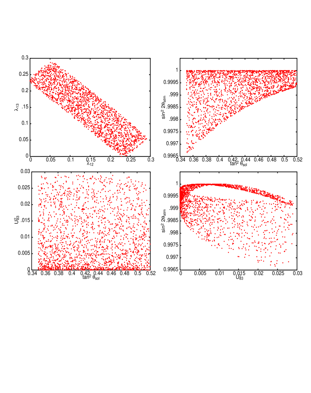
Figure 3: Scatter plot of the two $\lambda$ parameters and the oscillation parameters in the case of $\lambda_{23}=1$ for the 1$\sigma$ range of the neutrino mixing parameters given in Eq. (4). Conservation of CP is assumed.

The correlations of $\lambda_{12}$ and $\lambda_{13}$ as well as of the mixing parameters for $\lambda_{23}=1$ are shown in Fig. 3. We used the 1$\sigma$ allowed ranges of the oscillation parameters, Eq. (4). As Fig. 3 shows, $\sin^{2}2\theta_{\rm atm}$ is practically 1 in this case, $\sin^{2}2\theta_{\rm atm}\mathrel{\hbox to0.0pt{\raise 2.20013pt\hbox{$>$}\hss}{\lower 2.20013pt\hbox{$\sim$}}}0.9965$. The lower limit is reached for relatively large $|U_{e3}|^{2}\simeq 0.025$ and relatively small $\tan^{2}\theta_{\rm sol}\simeq 0.32$. However, such small deviations of $\sin^{2}2\theta_{\rm atm}$ from 1 are extremely difficult to measure . For $\lambda_{23}=1$ and “small” $\lambda_{12,13}$, $U_{\lambda}$ has the following structure:

$$\mbox{$U_{\lambda}$}\simeq\left(\begin{array}[]{ccc}1-\frac{1}{2}\,(\lambda_{12}^{2}+\lambda_{13}^{2})&\lambda_{12}&\lambda_{13}\\[5.69046pt] -\lambda_{13}&-\lambda_{12}\,\lambda_{13}&1-\frac{1}{2}\,\lambda_{13}^{2}\\[5.69046pt] \lambda_{12}&-1+\frac{1}{2}\,\lambda_{12}^{2}&0\end{array}\right)+{\cal O}(\lambda^{3})~{}.$$ (13)

All three possibilities $\lambda_{12}\gg\lambda_{13}$, $\lambda_{13}\gg\lambda_{12}$ and $\lambda_{12}\sim\lambda_{13}$ are allowed. In any of these three cases the 23 submatrix of $U_{\lambda}$ displays an antidiagonal structure, as seen in Eq. (13).

3.3 Large $\lambda_{ij}$

It is also possible that all $\lambda_{ij}=\sin\theta^{\prime}_{ij}$ are relatively large, $\lambda_{ij}\mathrel{\hbox to0.0pt{\raise 2.20013pt\hbox{$>$}\hss}{\lower 2.20013pt\hbox{$\sim$}}}0.40$. From Fig. 1 one sees that in this case $\lambda_{12}\simeq(0.92-0.99)~{}[0.85-0.99]$, $\lambda_{13}\simeq(0.57-0.77)~{}[0.47-0.85]$, and $\lambda_{23}\simeq(0.57-0.92)~{}[0.40-0.99]$, when the 1 s.d. [3 s.d.] ranges of the oscillation parameters are used. It turns out that, $\cos\theta^{\prime}_{23}>0$, whereas $\cos\theta^{\prime}_{12,13}$ can take both signs.

We limit our discussion to the case of all $\lambda_{ij}$ being “large”: $\lambda_{ij}\geq 1/\sqrt{2}$. We can use the deviations of $\lambda_{12}$ from 1, and the deviations of $\lambda_{13,23}$ from $1/\sqrt{2}$, as small parameters to get convenient expressions for $\tan^{2}\theta_{\rm sol}$, $|U_{e3}|^{2}$ and $\sin^{2}2\theta_{\rm atm}$:

$$\begin{array}[]{c}\lambda_{12}\equiv 1-\epsilon_{12}^{2}\\[8.5359pt] \lambda_{13}\equiv\frac{1}{\sqrt{2}}\,(1+\epsilon_{13}^{2})\\[8.5359pt] \lambda_{23}\equiv\frac{1}{\sqrt{2}}\,(1+\epsilon_{23}^{2})~{},\end{array}$$ (14)

where $\epsilon^{2}_{12}\mathrel{\hbox to0.0pt{\raise 2.20013pt\hbox{$<$}\hss}{\lower 2.20013pt\hbox{$\sim$}}}0.08~{}(0.15)$, $\epsilon^{2}_{23}\mathrel{\hbox to0.0pt{\raise 2.20013pt\hbox{$<$}\hss}{\lower 2.20013pt\hbox{$\sim$}}}0.30~{}(0.40)$ and $\epsilon^{2}_{13}\mathrel{\hbox to0.0pt{\raise 2.20013pt\hbox{$<$}\hss}{\lower 2.20013pt\hbox{$\sim$}}}0.09~{}(0.20)$, where the 1 s.d. (3 s.d.) ranges of the oscillation parameters were used. One obtains for sufficiently small $\epsilon_{ij}$:

$$\begin{array}[]{c}\tan^{2}\theta_{\rm sol}\simeq 1-4\,\epsilon_{12}+8\,\epsilon_{12}^{2}+{\cal O}(\epsilon^{3})~{},\\[8.5359pt] U_{e3}\simeq\epsilon_{23}^{2}-\epsilon_{12}+{\cal O}(\epsilon^{3})~{},\\[8.5359pt] \sin^{2}2\theta_{\rm atm}\simeq 1+{\cal O}(\epsilon^{4})~{}.\end{array}$$ (15)

The terms of higher order in $\epsilon$ we do not give can be sizable. The scatter plots do not show any new important correlation. In particular, $\mbox{$\sin^{2}2\theta_{\rm atm}$}{}\simeq 0.95$ is possible also in the case under discussion. Both $\epsilon_{23}$ and $\epsilon_{13}$ can be zero, whereas $\epsilon_{12}$ cannot. No hierarchy is implied. If $\epsilon_{12}\gg\epsilon_{13,23}$, we get $|U_{e3}|\simeq\epsilon_{12}(1-\epsilon^{2}_{12}/4)+{\cal O}(\epsilon^{4})$, and

$$\tan^{2}\theta_{\rm sol}\simeq 1-4~{}|U_{e3}|+8~{}|U_{e3}|^{2}-16~{}|U_{e3}|^{3}~{}.$$ (16)

For all $\lambda_{ij}$ “large”, $\lambda_{ij}\geq 1/\sqrt{2}$, $U_{\lambda}$ has the form:

$$\mbox{$U_{\lambda}$}\simeq\left(\begin{array}[]{ccc}\epsilon_{12}&\frac{1}{\sqrt{2}}-\frac{\epsilon_{12}^{2}+\epsilon_{13}^{2}}{\sqrt{2}}&\frac{1}{\sqrt{2}}+\frac{\epsilon_{13}^{2}}{\sqrt{2}}\\[5.69046pt] \frac{-1}{\sqrt{2}}-\frac{\epsilon_{12}}{\sqrt{2}}+\frac{\epsilon_{12}^{2}+\epsilon_{23}^{2}}{\sqrt{2}}&\frac{-1}{2}+\epsilon_{12}+\frac{1}{2}\,(\epsilon_{12}^{2}-\epsilon_{13}^{2}-\epsilon_{23}^{2})&\frac{1}{2}+\frac{1}{2}\,(\epsilon_{23}^{2}-\epsilon_{13}^{2})\\[5.69046pt] \frac{1}{\sqrt{2}}-\frac{\epsilon_{12}}{\sqrt{2}}+\frac{\epsilon_{23}^{2}-\epsilon_{12}^{2}}{\sqrt{2}}&\frac{-1}{2}-\epsilon_{12}+\frac{1}{2}\,(\epsilon_{12}^{2}-\epsilon_{13}^{2}+\epsilon_{23}^{2})&\frac{1}{2}-\frac{1}{2}\,(\epsilon_{23}^{2}+\epsilon_{13}^{2})\end{array}\right)+{\cal O}(\epsilon^{3})~{}.$$ (17)

All entries in $U_{\lambda}$, except the 11 entry, are large.

Let us summarize the results obtained under the assumption of CP–conservation:

• If all $\lambda_{ij}$ are small, one typically has $\mbox{$\tan^{2}\theta_{\rm sol}$}\mathrel{\hbox to0.0pt{\raise 2.20013pt\hbox{$>$}\hss}{\lower 2.20013pt\hbox{$\sim$}}}0.42$ and $|U_{e3}|^{2}\mathrel{\hbox to0.0pt{\raise 2.20013pt\hbox{$>$}\hss}{\lower 2.20013pt\hbox{$\sim$}}}0.02$. The matrix $U_{\lambda}$ has a “CKM–like” structure. One can have $\mbox{$\sin^{2}2\theta_{\rm atm}$}\simeq 0.95$, i.e., $\sin^{2}2\theta_{\rm atm}$ can deviate noticeably from 1.

• If $\lambda_{23}=1$ and $\lambda_{12,13}$ are small, one practically has $\mbox{$\sin^{2}2\theta_{\rm atm}$}{}\simeq 1$, the possible deviations from 1 being exceedingly small. Any deviation of $\sin^{2}2\theta_{\rm atm}$ from 1 would imply rather large $|U_{e3}|^{2}$ and relatively small $\tan^{2}\theta_{\rm sol}$. The 23 block of the matrix $U_{\lambda}$ has an antidiagonal (quasi–Dirac like) form.

• If all $\lambda_{ij}$ are large, $\lambda_{ij}\mathrel{\hbox to0.0pt{\raise 2.20013pt\hbox{$>$}\hss}{\lower 2.20013pt\hbox{$\sim$}}}1/\sqrt{2}$, the matrix $U_{\lambda}$ displays the unusual structure given in Eq. (17), with all elements, except the 11 element, being large. Also in this case we can have $\mbox{$\sin^{2}2\theta_{\rm atm}$}{}\simeq 0.95$.

3.4 Implied Forms of the Charged Lepton Mass Matrix

The matrix $U_{\lambda}$ arises from the diagonalization of the charged lepton mass matrix $m_{\rm lep}$. Having the approximate form of $U_{\lambda}$ and using the knowledge of the charged lepton masses $m_{e}$, $m_{\mu}$ and $m_{\tau}$, we can derive the structure of two different matrices related to $m_{\rm lep}$. The first one is the matrix $m_{\rm lep}~{}m_{\rm lep}^{\dagger}$, which is diagonalized by $U_{\lambda}$, i.e.,

$$m_{\rm lep}~{}m_{\rm lep}^{\dagger}=\mbox{$U_{\lambda}$}~{}(m_{\rm lep}^{\rm diag})^{2}~{}\mbox{$U_{\lambda}$}^{\dagger}~{},$$ (18)

where $m_{\rm lep}^{\rm diag}$ is a diagonal mass matrix containing the charged lepton masses $m_{e}$, $m_{\mu}$ and $m_{\tau}$. The second matrix is

$$\mbox{$U_{\lambda}$}~{}m_{\rm lep}^{\rm diag}~{}\mbox{$U_{\lambda}$}^{T}~{}.$$ (19)

Under the assumption of $m_{\rm lep}$ being symmetric, which is realized in some GUT theories, the matrix in Eq. (19) coincides with the charged lepton mass matrix.

Consider first the matrix $m_{\rm lep}~{}m_{\rm lep}^{\dagger}$. In the case of “small” $\lambda_{ij}$, we find that

$$m_{\rm lep}~{}m_{\rm lep}^{\dagger}\simeq\left(\begin{array}[]{ccc}m_{e}^{2}+m_{\tau}^{2}~{}\lambda_{13}^{2}+m_{\mu}^{2}~{}\lambda_{12}^{2}&m_{\tau}^{2}~{}\lambda_{13}~{}\lambda_{23}+m_{\mu}^{2}~{}\lambda_{12}&m_{\tau}^{2}~{}\lambda_{13}-m_{\mu}^{2}~{}\lambda_{12}~{}\lambda_{13}\\[8.5359pt] \cdot&m_{\mu}^{2}+m_{\tau}^{2}~{}\lambda_{23}^{2}&m_{\tau}^{2}\lambda_{23}-m_{\mu}^{2}~{}\lambda_{12}~{}\lambda_{13}\\[8.5359pt] \cdot&\cdot&m_{\tau}^{2}\end{array}\right)~{}$$ (20)

plus terms of order $\lambda^{3}$. Thus, $m_{\rm lep}~{}m_{\rm lep}^{\dagger}$ is close to a diagonal matrix. In the special case of $\lambda_{13}=\lambda_{23}\simeq 0$ we get:

$$m_{\rm lep}~{}m_{\rm lep}^{\dagger}\simeq\left(\begin{array}[]{ccc}m_{e}^{2}+m_{\mu}^{2}~{}\lambda^{2}&m_{\mu}^{2}~{}\lambda&0\\[8.5359pt] m_{\mu}^{2}~{}\lambda&m_{\mu}^{2}&0\\[8.5359pt] 0&0&m_{\tau}^{2}\end{array}\right)~{}.$$ (21)

The zero entries can be terms of order $m^{2}_{e}$. The matrix $m_{\rm lep}~{}m_{\rm lep}^{\dagger}$ has clearly a hierarchical structure.

When $\lambda_{23}=1$ and $\lambda_{12,13}$ are “small”, one obtains:

$$m_{\rm lep}~{}m_{\rm lep}^{\dagger}\simeq\left(\begin{array}[]{ccc}m_{e}^{2}+m_{\tau}^{2}~{}\lambda_{13}^{2}+m_{\mu}^{2}~{}\lambda_{12}^{2}&m_{\tau}^{2}~{}\lambda_{13}&-m_{\mu}^{2}~{}\lambda_{12}\\[8.5359pt] m_{\tau}^{2}~{}\lambda_{13}&m_{\tau}^{2}&m_{\mu}^{2}~{}\lambda_{12}~{}\lambda_{13}\\[8.5359pt] -m_{\mu}^{2}~{}\lambda_{12}&m_{\mu}^{2}~{}\lambda_{12}~{}\lambda_{13}&m_{\mu}^{2}\end{array}\right)~{}.$$ (22)

In contrast to the previous case, now the 22 element is equal to $m_{\tau}^{2}$ and the 33 element is given by $m_{\mu}^{2}$. The 12 block of $m_{\rm lep}~{}m_{\rm lep}^{\dagger}$ is hierarchical, while the 23 block has “inverted hierarchy–like” form.

Finally, if all $\lambda_{ij}$ are “large”, we can expect that $m_{\rm lep}~{}m_{\rm lep}^{\dagger}$ is to a good approximation a “democratic” matrix. Indeed, one finds:

$$m_{\rm lep}~{}m_{\rm lep}^{\dagger}\simeq\frac{m_{\tau}^{2}}{2}~{}\left(\begin{array}[]{ccc}1&1/\sqrt{2}&1/\sqrt{2}\\[8.5359pt] 1/\sqrt{2}&1/2&1/2\\[8.5359pt] 1/\sqrt{2}&1/2&1/2\end{array}\right)$$ (23)

plus terms of order $\epsilon$.

From the definition of the two characteristic mass matrices in Eqs. (18) and (19) it follows that the expressions for $\mbox{$U_{\lambda}$}~{}m_{\rm lep}^{\rm diag}~{}\mbox{$U_{\lambda}$}^{T}$ in the three cases we are discussing can be obtained from the corresponding expressions of $m_{\rm lep}~{}m_{\rm lep}^{\dagger}$ given above by replacing $m_{l}^{2}$ with $m_{l}$ in the latter.

4 CP Nonconservation

4.1 General Considerations

It is well known that if the neutrinos with definite mass are Majorana particles, the PMNS matrix contains 6 physical parameters, three mixing angles, and three CP–violating phases. The latter can be divided in one “Dirac phase”, $\delta$, and two “Majorana phases”, $\alpha$ and $\beta$. The Majorana phases appear only in amplitudes describing lepton number violating processes in which the total lepton charge changes by two units. In general, as we have already discussed, one has

$$\mbox{$U_{\rm PMNS}$}=U_{\rm lep}^{\dagger}\,U_{\nu}~{}.$$ (24)

where $U_{\rm lep}$ and $U_{\nu}$ two $3\times 3$ unitary matrices: $U_{\rm lep}$ arises from the diagonalization of the charged lepton mass matrix, while $U_{\nu}$ diagonalizes the neutrino Majorana mass term. Any $3\times 3$ unitary matrix contains 3 moduli and 6 phases and can be written as [26]

$$U=e^{i\Phi}\,P\,\tilde{U}\,Q~{},$$ (25)

where $P\equiv{\rm diag}(1,e^{i\phi_{1}},e^{i\phi_{2}})$ and $Q\equiv{\rm diag}(1,e^{i\rho_{1}},e^{i\rho_{2}})$ are diagonal phase matrices having 2 phases each, and $\tilde{U}$ is a unitary “CKM–like” matrix containing 1 phase and 3 angles. The charged lepton Dirac mass term, $m_{\rm lep}$, is diagonalized by a bi–unitary transformation:

$$m_{\rm lep}=U_{L}\,m_{\rm lep}^{\rm diag}\,U_{R}^{\dagger}~{},$$ (26)

where $U_{L,R}$ are $3\times 3$ unitary matrices and $m_{\rm lep}^{\rm diag}$ is the diagonal matrix containing the masses of the charged leptons. Casting $U_{L,R}$ in the form (25), i.e., $U_{L,R}=e^{i\Phi_{L,R}}\,P_{L,R}\,\tilde{U}_{L,R}\,Q_{L,R}$, we find

$$m_{\rm lep}=e^{i(\Phi_{L}-\Phi_{R})}\,Q_{L}\,\tilde{U}_{L}\,P_{L}\,m_{\rm lep}^{\rm diag}\,Q_{R}^{\dagger}\,\tilde{U}_{R}^{\dagger}\,P_{R}^{\dagger}~{}.$$ (27)

The term $P_{L}\,m_{\rm lep}^{\rm diag}\,Q_{R}^{\dagger}$ contains only 2 relative phases, which can be associated with the right–handed charged lepton fields. The three independent phases in $e^{i(\Phi_{L}-\Phi_{R})}\,Q_{L}$ can be absorbed by a redefinition of the left–handed charged lepton fields. Therefore, $U_{\rm lep}$ is effectively given by $\tilde{U}_{L}$ and contains three angles and one phase.

The neutrino mass matrix $m_{\nu}$ is diagonalized via

$$m_{\nu}=U_{\nu}\,m_{\nu}^{\rm diag}\,U_{\nu}^{T}~{}.$$ (28)

The unitary matrix $U_{\nu}$ can be written in the form (25). It is not possible to absorb phases in the neutrino fields since the neutrino mass term is of Majorana type [16, 17]. Thus,

$$\mbox{$U_{\rm PMNS}$}=U_{\rm lep}^{\dagger}\,U_{\nu}=e^{i\Phi\nu}\,\tilde{U}_{\rm lep}^{\dagger}\,P_{\nu}\,\tilde{U}_{\nu}\,Q_{\nu}~{}.$$ (29)

The common phase $\Phi_{\nu}$ has no physical meaning and we will ignore it. Consequently, in the most general case, the elements of $U_{\rm PMNS}$ given by Eq. (29) are expressed in terms of six real parameters and six phases in $\tilde{U}_{\rm lep}$ and $U_{\nu}$  . Only six combinations of those — the three angles and the three phases of $U_{\rm PMNS}$, are observable, in principle, at low energies. Note that the two phases in $Q_{\nu}$ are “Majorana–like”, since they will not appear in the probabilities describing the flavour neutrino oscillations [16, 19]. Note also that if $U_{\rm lep}={\mathbbm{1}}$, the phases in the matrix $P_{\nu}$ can be eliminated by a redefinition of the charged lepton fields.

The requirement of bimaximality of $\tilde{U}_{\nu}$ implies that $\tilde{U}_{\nu}$ is real and given by Eq. (1). In this case the three angles and the Dirac phase in the PMNS matrix $U_{\rm PMNS}$ will depend in a complicated manner on the three angles and the phase in $\tilde{U}_{\rm lep}$ and on the two phases in $P_{\nu}$. The two Majorana phases will depend in addition on the parameters in $Q_{\nu}$.

It should be emphasized that the form of $U_{\rm PMNS}$ given in Eq. (29) is the most general one. A specific model in the framework of which the bimaximal $\tilde{U}_{\nu}$ is obtained, might imply symmetries or textures, along the lines of, e.g., [33], in $m_{\nu}$, which will reduce the number of independent parameters in $U_{\nu}$. We will comment in Section 4.6 on such possibilities.

In the scheme with three massive Majorana neutrinos under discussion there exist three rephasing invariants related to the three CP–violating phases in ${\rm U_{\rm PMNS}}$, $\delta$, $\alpha$ and $\beta$ [27, 28, 29, 30, 31]. The first is the standard Dirac one $J_{CP}$ [27], associated with the Dirac phase $\delta$:

$$J_{CP}={\rm Im}\left\{U_{e1}\,U_{\mu 2}\,U_{e2}^{\ast}\,U_{\mu 1}^{\ast}\right\}~{}.$$ (30)

It determines the magnitude of CP–violation effects in neutrino oscillations [28]. Let us note that if $U_{\rm lep}={\mathbbm{1}}$ and $\tilde{U_{\nu}}$ is a real matrix, one has $J_{CP}=0$.

The two additional invariants, $S_{1}$ and $S_{2}$, whose existence is related to the Majorana nature of massive neutrinos, i.e., to the phases $\alpha$ and $\beta$, can be chosen as [29, 31] (see also [21]) :

$$S_{1}={\rm Im}\left\{U_{e1}\,U_{e3}^{\ast}\right\}~{},~{}~{}~{}~{}S_{2}={\rm Im}\left\{U_{e2}\,U_{e3}^{\ast}\right\}~{}.$$ (31)

If $S_{1}\neq 0$ and/or $S_{2}\neq 0$, CP is not conserved due to the Majorana phases $\beta$ and/or $(\alpha-\beta)$. The effective Majorana mass in $(\beta\beta)_{0\nu}$–decay, $\left|<\!m\!>\right|$, depends, in general, on $S_{1}$ and $S_{2}$ [21] and not on $J_{CP}$. Let us note, however, even if $S_{1,2}=0$ (which can take place if, e.g., $|U_{e3}|=0$), the two Majorana phases $\alpha$ and $\beta$ can still be a source of CP–nonconservation in the lepton sector provided ${\rm Im}\left\{U_{e1}\,U_{e2}^{\ast}\right\}\neq 0$ and ${\rm Im}\left\{U_{\mu 2}\,U_{\mu 3}^{\ast}\right\}\neq 0$ [31, 32].

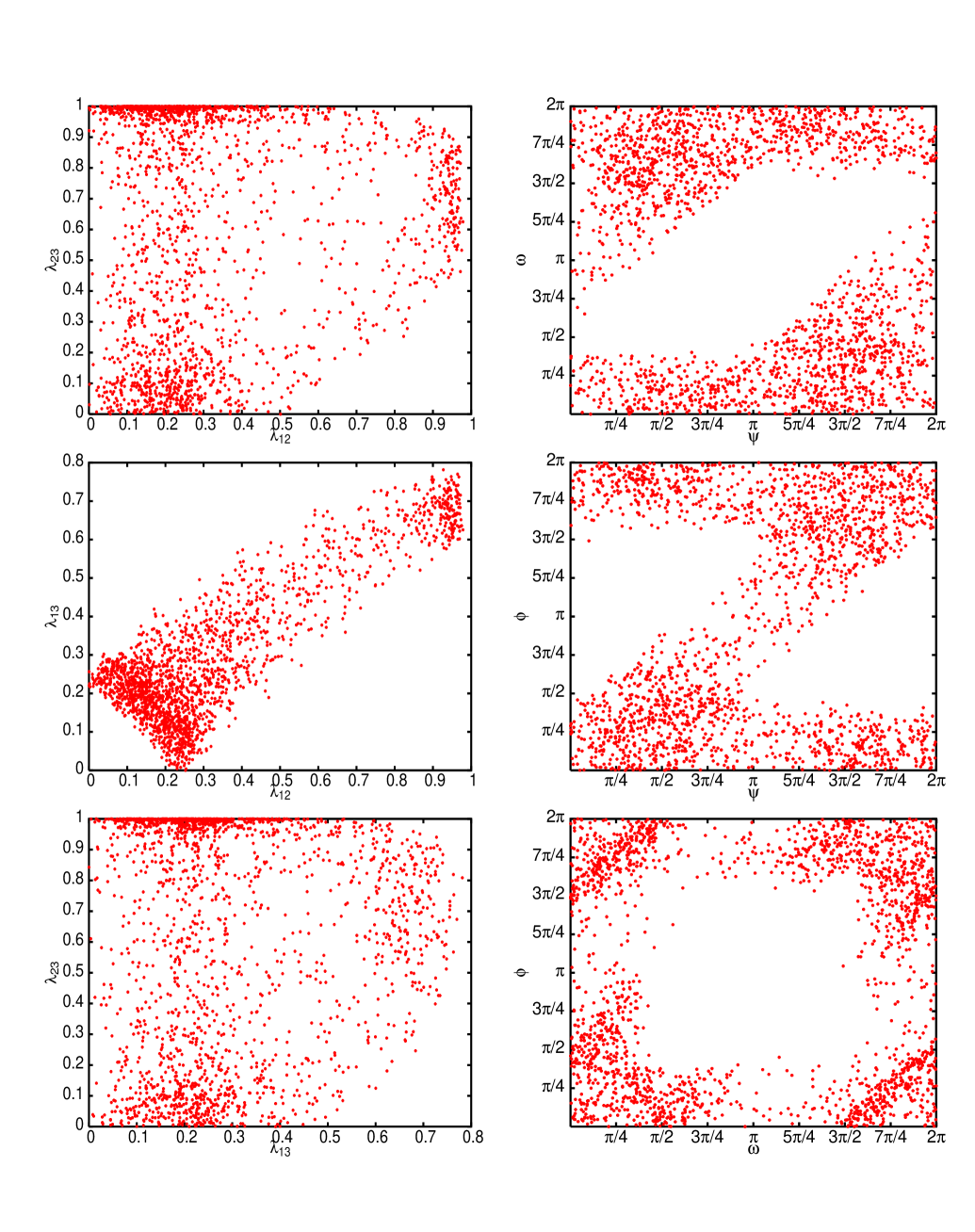
Figure 4: Scatter plot of the three $\lambda$ parameters and the CP–violating phases for the 1$\sigma$ allowed ranges of values of the neutrino mixing parameters given in Eq. (4).

Let us denote the phase in $\tilde{U}_{\rm lep}$ by $\psi$. We will include it in $\tilde{U}_{\rm lep}$ in the same way this is done for the phase $\delta$ in Eq. (3). We will also use $P_{\nu}={\rm diag}(1,e^{i\phi},e^{i\omega})$ and $Q_{\nu}\equiv{\rm diag}(1,e^{i\rho},e^{i\sigma})$. This means that the Dirac phase $\delta$, which has observable consequences in neutrino oscillation experiments, is determined only by the phases $\psi$, $\phi$ and $\omega$. The Majorana phases in $U_{\rm PMNS}$, $\alpha$ and $\beta$, receive contributions also from the two remaining phases $\rho$ and $\sigma$. Allowing the phases $\delta$, $\alpha$ and $\beta$ to vary between 0 and $2\pi$, permits to constrain (without loss of generality) the mixing angles $\theta_{ij}$ to lie between 0 and $\pi/2$. In Fig. 4 we show the result of a random search for the allowed regions of the values of the parameters $\lambda_{ij}$. The regions present in Fig. 1 are again allowed. Clustering of points around these regions is also observed. The effect of the phases is that values of the parameters, located in areas between the regions corresponding to the case of CP–conservation are allowed. Let us consider the physical observables of interest in the three main regions of the parameter space we have identified earlier.

4.2 Small $\lambda_{ij}$

Let us choose $\lambda_{12}=\lambda$, $\lambda_{23}=A\,\lambda$ and $\lambda_{13}=B\,\lambda$ with $A,B$ real and of order one . In this case $\tan^{2}\theta_{\rm sol}$, $U_{e3}$ and $\sin^{2}2\theta_{\rm atm}$ are given by

$$\begin{array}[]{c}\tan^{2}\theta_{\rm sol}\simeq 1-2\sqrt{2}\,(c_{\phi}-B\,c_{\omega-\psi})\,\lambda+2\left(2\,(c_{\phi}-B\,c_{\omega-\psi})^{2}-\sqrt{2}\,A\,(c_{\omega}+B\,c_{\phi-\psi})\right)\,\lambda^{2}~{},\\[8.5359pt] U_{e3}\simeq\sqrt{\frac{\displaystyle 1}{\displaystyle 2}(\displaystyle 1+B^{2}+2\,B\,c_{\omega-\phi-\psi})}\left(\lambda~{}-~{}\frac{\displaystyle(1-B^{2})\,A\,c_{\omega-\phi}}{\displaystyle 1+B^{2}+2\,B\,c_{\omega-\phi-\psi}}\,\lambda^{2}\right)~{},\\[8.5359pt] \sin^{2}2\theta_{\rm atm}\simeq 1-4\,A^{2}\,c_{\omega-\phi}\,\lambda^{2}\end{array}$$ (32)

plus terms of order ${\cal{O}}(\lambda^{3})$. We introduced the obvious notation $c_{\phi}=\cos\phi$, $s_{\omega-\psi}=\sin(\omega-\psi)$, etc. Note that the possibility of all three $\lambda_{ij}$ being of the same order was not possible in case of conservation of CP. The rephasing invariant $J_{CP}$, which controls the magnitude of CP–violating effects in neutrino oscillations, has the form:

$$J_{CP}\simeq\frac{\lambda}{4\sqrt{2}}\,\left(s_{\phi}+B\,s_{\omega-\psi}+\lambda\,(s_{\omega-2\phi}+B\,s_{2\omega-\phi-\psi})\,A\right)+{\cal{O}}(\lambda^{3})~{}.$$ (33)

Thus, not only the phase $\psi$ of $\tilde{U}_{\rm lep}$, but also the phases $\omega$ and $\phi$ from $P_{\nu}$ contribute to $J_{CP}$. Using Eqs. (32) and (33) it is not difficult to convince oneself that the magnitude of $J_{CP}$ is controlled by the magnitude of $|U_{e3}|$. Indeed, if, e.g., $c_{\omega-\phi-\psi}=-1$ and $B=1$, so that the term $\sim\lambda$ in the expression for $U_{e3}$ vanishes and to leading order $U_{e3}\simeq-\sqrt{2}\,A\,c_{\omega-\phi}\,\lambda^{2}$, the term $\sim\lambda$ in $J_{CP}$ also vanishes and we have $J_{CP}\sim U_{e3}$.

The invariants $S_{1}$ and $S_{2}$ which (for $|U_{e3}|\neq 0$) determine the magnitude of the effects of CP–violation associated with the Majorana nature of massive neutrinos, read:

$$\begin{array}[]{c}S_{1}\simeq\frac{\displaystyle\lambda}{\displaystyle 2}\left(s_{\phi+\sigma}+B\,s_{\omega-\psi+\sigma}\right)\\[8.5359pt] S_{2}\simeq\frac{\displaystyle\lambda}{\displaystyle 2}\left(s_{\phi-\rho+\sigma}+B\,s_{\omega-\psi-\rho+\sigma}\right)~{},\end{array}$$ (34)

where we gave only the terms of order $\lambda$. We see that all five phases in $\tilde{U}_{\rm lep}$, $P_{\nu}$ and $Q_{\nu}$, and not only the phases $\rho$ and $\sigma$ in $Q_{\nu}$, contribute to $S_{1}$ and $S_{2}$. In the leading order expressions for $S_{1,2}$, Eq. (34), the five phases enter in three independent combinations. Moreover, in the case of $\rho=\sigma=0$, which is realized if the bimaximal mixing structure of $U_{\nu}$ is associated (in the limit of $U_{\rm lep}={\mathbbm{1}}$) with the approximate conservation of $L^{\prime}=L_{e}-L_{\mu}-L_{\tau}$ (see Subsection 4.6), we have to leading order in $\lambda$:

$$J_{CP}\simeq\frac{S_{1}}{2\,\sqrt{2}}\simeq\frac{S_{2}}{2\,\sqrt{2}}~{}.$$ (35)

Thus, the magnitude of the CP–violating effects in neutrino oscillations is directly related in this case to the magnitude of the CP–violating effects associated with the Majorana nature of neutrinos. To leading order, both types of CP–violating effects are due to two phases, $\phi$ and $(\omega-\psi)$. We will consider a model in which $\rho=\sigma=0$ in Subsection 4.6.

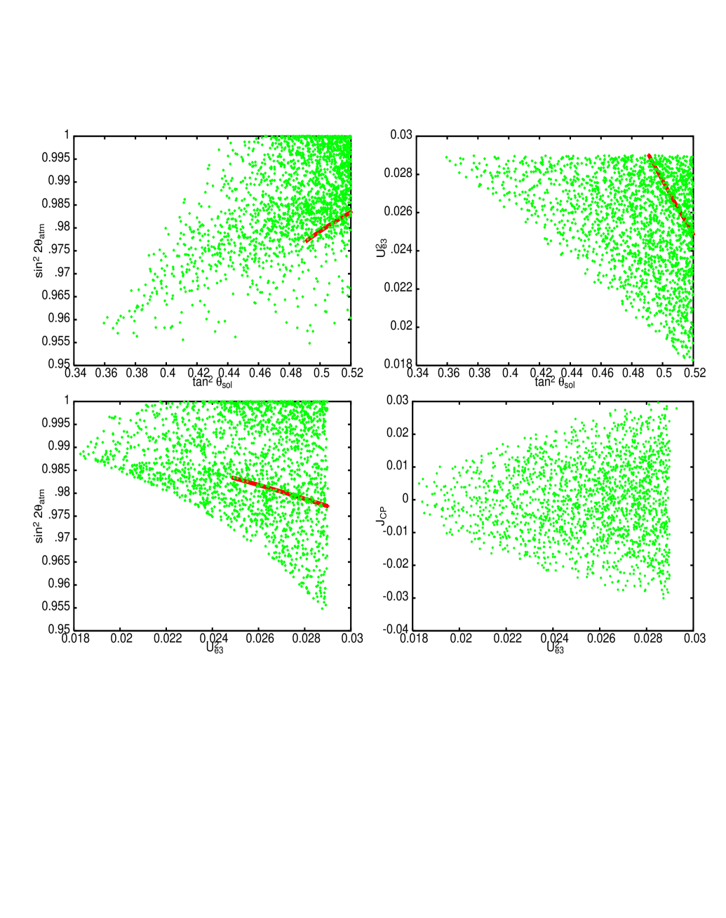
Figure 5: Scatter plot of the oscillation parameters for the case of hierarchical $\lambda_{ij}$, i.e., $\lambda_{13}=\lambda_{12}\,\lambda_{23}=\lambda_{12}^{3}$. The various possible regions and correlations are shown both in the case of CP–violation (bright green areas) and CP–conservation (dark red areas). The 1$\sigma$ allowed ranges of values of the neutrino mixing parameters given in Eq. (4) were used.

In Fig. 5 we show the correlations between the observables $\tan^{2}\theta_{\rm sol}$, $|U_{e3}|^{2}$ and $\sin^{2}2\theta_{\rm atm}$, when a hierarchy between the three $\lambda$ parameters of the form we have considered in Subsection 3.2, $\lambda_{12}\equiv\lambda$, $\lambda_{13}=\lambda^{3}$ and $\lambda_{23}=\lambda^{2}$, is assumed. The $1\sigma$ allowed ranges of $\tan^{2}\theta_{\rm sol}$, $|U_{e3}|^{2}$ and $\sin^{2}2\theta_{\rm atm}$, were used to constrain $\lambda$ and the CP–violating phases. As it follows from Fig. 5, $\tan^{2}\theta_{\rm sol}$ can take values in the whole $1\sigma$ interval allowed by the data, Eq. (4). This is in sharp contrast to the case of CP–conservation, in which the correlation between the values $|U_{e3}|$ and the deviation of $\tan^{2}\theta_{\rm sol}$ from 1 leads, as Fig. 5 shows, to the lower limit $\mbox{$\tan^{2}\theta_{\rm sol}$}\mathrel{\hbox to0.0pt{\raise 2.20013pt\hbox{$>$}\hss}{\lower 2.20013pt\hbox{$\sim$}}}0.48$. We find also that if CP is not conserved, the following lower bound holds: $|U_{e3}|^{2}\mathrel{\hbox to0.0pt{\raise 2.20013pt\hbox{$>$}\hss}{\lower 2.20013pt\hbox{$\sim$}}}0.018$. There are interesting correlations between $\tan^{2}\theta_{\rm sol}$, $|U_{e3}|^{2}$ and $\sin^{2}2\theta_{\rm atm}$. For instance, $\mbox{$\tan^{2}\theta_{\rm sol}$}{}\leq 0.40$ implies $|U_{e3}|^{2}\mathrel{\hbox to0.0pt{\raise 2.20013pt\hbox{$>$}\hss}{\lower 2.20013pt\hbox{$\sim$}}}0.026$ and $\mbox{$\sin^{2}2\theta_{\rm atm}$}\mathrel{\hbox to0.0pt{\raise 2.20013pt\hbox{$<$}\hss}{\lower 2.20013pt\hbox{$\sim$}}}0.975$.

4.3 The Case of $\lambda_{23}=1$

This case corresponds to “small” $\lambda_{12,13}$, $\lambda_{12,13}\mathrel{\hbox to0.0pt{\raise 2.20013pt\hbox{$<$}\hss}{\lower 2.20013pt\hbox{$\sim$}}}0.35$. Introducing $\lambda_{12}=\lambda$ and $\lambda_{13}=B\lambda$, with $B$ real, we find:

$$\begin{array}[]{c}\tan^{2}\theta_{\rm sol}\simeq 1-2\sqrt{2}\,(c_{\omega}+B\,c_{\phi-\psi})\,\lambda+4\left(c_{\omega}+B\,c_{\omega-\psi}\right)^{2}\,\lambda^{2}~{},\\[8.5359pt] U_{e3}\simeq\lambda\,\sqrt{\frac{\displaystyle 1}{\displaystyle 2}(1+B^{2}-2\,B\,c_{\omega-\phi+\psi})}+{\cal O}(\lambda^{3})~{},\\[8.5359pt] \sin^{2}2\theta_{\rm atm}\simeq 1-\frac{1}{4}\,(1-B^{2}-2\,B\,c_{\omega-\phi-\psi})^{2}\,\lambda^{4}~{}.\end{array}$$ (36)

The formulae for the mixing parameters can actually be obtained from the corresponding formulae for all $\lambda_{ij}$ small, Eq. (32), by setting $A=0$ and making the change $B\rightarrow-B$, $\phi\leftrightarrow\omega$. The rephasing invariant $J_{CP}$ reads:

$$J_{CP}\simeq\frac{\lambda}{4\sqrt{2}}\,\left(s_{\omega}-B\,s_{\phi-\psi}\right)+{\cal O}(\lambda^{3})~{}.$$ (37)

The Majorana counterparts to $J_{CP}$, $S_{1}$ and $S_{2}$, are given by

$$\begin{array}[]{c}S_{1}\simeq-\frac{\displaystyle\lambda}{\displaystyle 2}\,\left(s_{\omega+\sigma}-B\,s_{\phi-\psi+\sigma}\right)\\[8.5359pt] S_{2}\simeq-\frac{\displaystyle\lambda}{\displaystyle 2}\,\left(s_{\omega-\rho+\sigma}-B\,s_{\phi-\psi-\rho+\sigma}\right)~{}.\end{array}$$ (38)

For $\rho=\sigma=0$ one finds that to order $\lambda$ the relation $S_{1}=S_{2}=-2\sqrt{2}~{}J_{CP}$ is valid. Relatively small $\omega$ is favored in this case. Furthermore, atmospheric neutrino mixing is predicted to be close to maximal, to be more precise, the lower limit $\mbox{$\sin^{2}2\theta_{\rm atm}$}\mathrel{\hbox to0.0pt{\raise 2.20013pt\hbox{$>$}\hss}{\lower 2.20013pt\hbox{$\sim$}}}0.97$ holds.

4.4 Large $\lambda_{ij}$

We consider $\lambda_{ij}\geq 1/\sqrt{2}$ and choose again as small expansion parameters the $\epsilon_{ij}$ introduced in Eq. (14). For the oscillation observables one finds

$$\begin{array}[]{c}\tan^{2}\theta_{\rm sol}\simeq 1-4\,\frac{\displaystyle\cos(\omega+\phi)/2}{\displaystyle\cos(\omega-\phi)/2}\,\epsilon_{12}+2\,\frac{\displaystyle 2+2\,c_{\omega+\phi}+c_{\omega+\psi}-c_{\phi+\psi}}{\displaystyle\cos^{2}(\omega-\phi)/2}\,\epsilon_{12}^{2}~{},\\[8.5359pt] U_{e3}\simeq\sin(\omega-\phi)/2+\epsilon_{12}\,\cos(\omega-\phi)/2~{},\\[8.5359pt] \sin^{2}2\theta_{\rm atm}\simeq 1+{\cal{O}}(\epsilon^{4})~{}.\end{array}$$ (39)

The atmospheric neutrino mixing is again very close to maximal. The term $\sim\sin(\omega-\phi)/2$ in $U_{e3}$ is not suppressed by positive powers of $\epsilon_{ij}$. This suggests that $(\omega-\phi)/2$ should be relatively small. For $\omega=\phi$ the expressions for the three rephasing invariants, associated with CP–nonconservation, take a rather simple form:

$$J_{CP}\simeq-\frac{s_{\phi}}{4}\,\epsilon_{12}+\frac{s_{\phi-\psi}}{4}\,\epsilon_{23}^{2}~{},$$ (40)

and

$$\begin{array}[]{c}S_{1}\simeq-\frac{\displaystyle s_{\psi-\sigma}}{\displaystyle\sqrt{2}}\,\epsilon_{12}-\frac{\displaystyle s_{\sigma}}{\displaystyle\sqrt{2}}\,\epsilon_{23}^{2}~{},\\[8.5359pt] S_{2}\simeq\frac{\displaystyle s_{\psi+\rho-\sigma}}{\displaystyle\sqrt{2}}\,\epsilon_{12}-\frac{\displaystyle s_{\rho-\sigma}}{\displaystyle\sqrt{2}}\,\epsilon_{23}^{2}~{}.\end{array}$$ (41)

In the case of $\sigma=\rho=0$ we have $S_{1}\simeq-S_{2}$, but there is no simple relation between $S_{1,2}$ and $J_{CP}$.

Note that in all three cases under study the connection between $S_{1}$, $S_{2}$ and $J_{CP}$ is different.

4.5 Special Cases

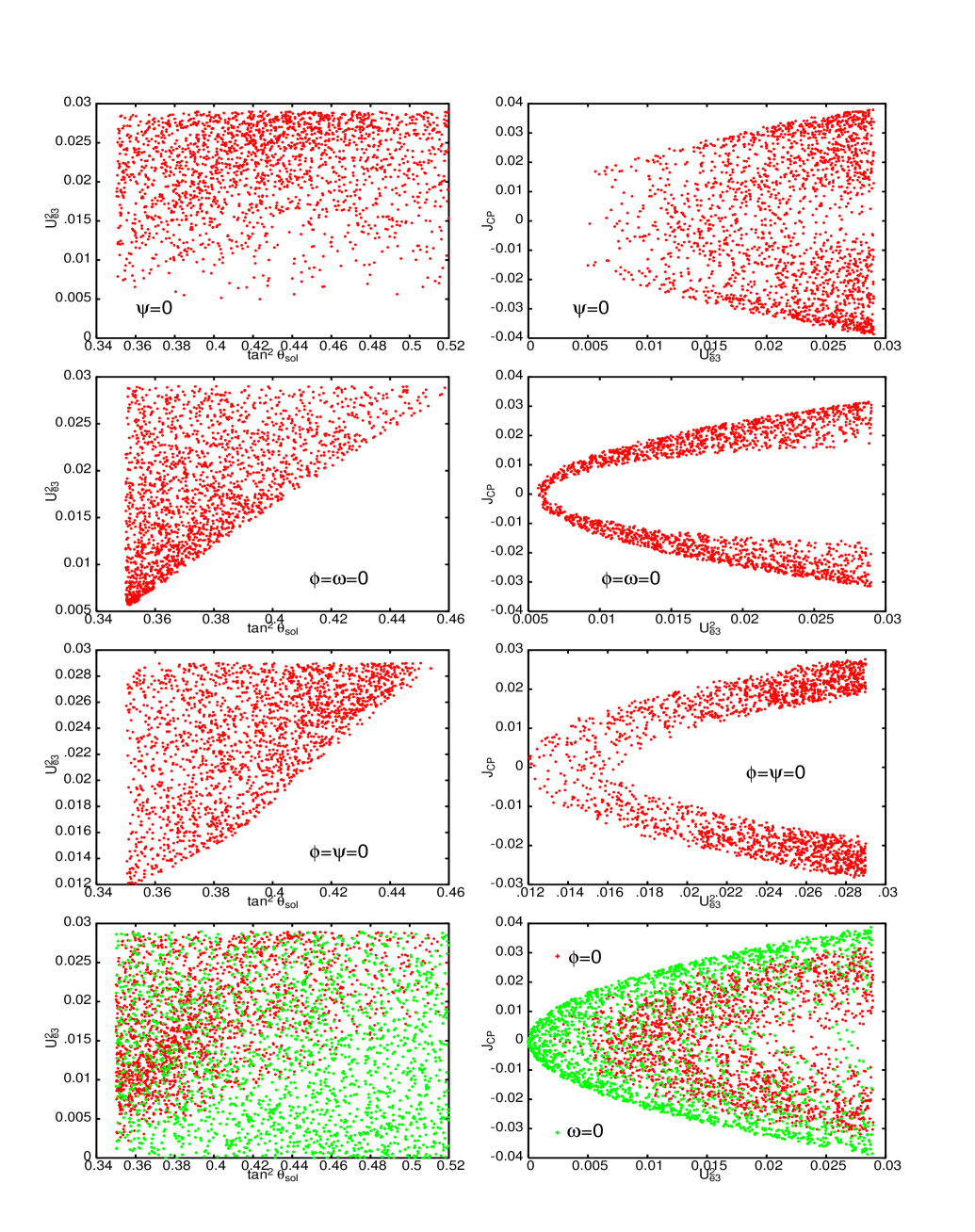
Figure 6: Scatter plot of the correlations between $\tan^{2}\theta_{\rm sol}$ and $|U_{e3}|^{2}$, and between $J_{CP}$ and $|U_{e3}|^{2}$, when the $\lambda_{ij}$ are of the same order and some of the CP–violating phases, $\psi$, $\phi$ and $\omega$, are zero. In the last row we display the CP–violating cases corresponding to $\omega=0$ (bright green areas) and $\phi=0$ (dark red area). The value $\lambda_{12}=0.24$ and 1$\sigma$ allowed ranges of values of the neutrino mixing parameters given in Eq. (4) were used.

It is instructive to examine the interplay of parameters when some of the three phases in $\tilde{U}_{\rm lep}$ and $P_{\nu}$ are zero. It turns out that there are no drastic consequences in the cases of “small” hierarchical $\lambda_{ij}$, of $\lambda_{23}=1$, and when all $\lambda_{ij}$ are “large”. Interesting correlations happen, however, in the case of “small” $\lambda_{ij}$ when the three $\lambda_{ij}$ are of the same order. To illustrate this we choose again $\lambda_{12}=\lambda$, $\lambda_{23}=A\,\lambda$ and $\lambda_{13}=B\,\lambda$ with $A,B$ real and of order one. We fix $\lambda=\sqrt{m_{\mu}/m_{\tau}}\simeq 0.24$ and vary $A,B$ between 0.4 and $1/\sqrt{\lambda}$. In doing so we observe that values of $A$ and $B$ slightly below 0.5 are favored, indicating a mild hierarchy in $\lambda_{ij}$. Inspecting Eq. (32) one finds that the dependence on $\omega$ of the oscillation parameters is rather weak. If $\omega=\psi$ one finds from Eq. (32) that $\tan^{2}\theta_{\rm sol}$ will be too large, $\mbox{$\tan^{2}\theta_{\rm sol}$}\mathrel{\hbox to0.0pt{\raise 2.20013pt\hbox{$>$}\hss}{\lower 2.20013pt\hbox{$\sim$}}}0.58$. We show in Fig. 6 the scatter plots of the correlations between $\tan^{2}\theta_{\rm sol}$ and $|U_{e3}|^{2}$, and between $|U_{e3}|^{2}$ and $J_{CP}$, which turn out to be the most interesting ones. The 1$\sigma$ allowed ranges of values of the neutrino mixing parameters given in Eq. (4) were used. If the charged lepton mass Lagrangian conserves CP, i.e., if $\psi=0$, there exists a lower bound on $|U_{e3}|^{2}\mathrel{\hbox to0.0pt{\raise 2.20013pt\hbox{$>$}\hss}{\lower 2.20013pt\hbox{$\sim$}}}0.005$. In this case $|J_{CP}|$ can be relatively large, for instance, $|J_{CP}|\simeq 0.035$ for $|U_{e3}|^{2}=0.025$, but is also allowed to be zero.

If CP is conserved by the neutrino mass term, i.e., if $\phi=\omega=0$, a simple correlation between $\tan^{2}\theta_{\rm sol}$ and $|U_{e3}|^{2}$ exists again: smaller $|U_{e3}|^{2}$ implies smaller $\tan^{2}\theta_{\rm sol}$ (see Fig. 6). A similar limit on $|U_{e3}|^{2}$ as in the case of $\psi=0$ applies. Most remarkably, the area of allowed values of $J_{CP}$ “bifurcates” as a function of $|U_{e3}|^{2}$ and for values of $|U_{e3}|^{2}\mathrel{\hbox to0.0pt{\raise 2.20013pt\hbox{$>$}\hss}{\lower 2.20013pt\hbox{$\sim$}}}0.008$, $J_{CP}=0$ is no longer allowed. For $|U_{e3}|^{2}\geq 0.010$, for instance, one has $|J_{CP}|\mathrel{\hbox to0.0pt{\raise 2.20013pt\hbox{$>$}\hss}{\lower 2.20013pt\hbox{$\sim$}}}0.01$. This can be understood as follows. If $\omega=\phi=0$ holds, the requirement of vanishing $J_{CP}$ (see Eq. (33)) is fulfilled for $\psi=0$. Then, one sees from Eq. (32) that to order $\lambda$, the equality

$$\mbox{$\tan^{2}\theta_{\rm sol}$}\simeq 1-4\,\frac{1-B}{1+B}\,|U_{e3}|$$ (42)

holds. For the values of $B$ considered, $B=(0.40-2.0)$, this equality is incompatible with the 1$\sigma$ upper bounds on $\tan^{2}\theta_{\rm sol}$ and $|U_{e3}|^{2}$.

The “bifurcation” happens also when $\phi=\psi=0$ holds (Fig. 6). The lower limit on $|U_{e3}|^{2}$ in this case is roughly by a factor of 4 smaller than in the preceding ones. Though not shown here, there can also be interesting constraints on $\sin^{2}2\theta_{\rm atm}$ when some of the phases vanish. If, e.g., $\omega=\phi=0$ holds, one sees from Eq. (32) that $1-\mbox{$\sin^{2}2\theta_{\rm atm}$}$ receives a correction of order $\lambda^{2}\simeq 0.06$. It can be shown that typically $\mbox{$\sin^{2}2\theta_{\rm atm}$}\mathrel{\hbox to0.0pt{\raise 2.20013pt\hbox{$<$}\hss}{\lower 2.20013pt\hbox{$\sim$}}}0.98$ in this case.

4.6 Specific Models

We shall consider next specific models in which Eq. (24) arises. We will also investigate how the CP–violating phases appear in the matrix $U_{\nu}$.

It is well–known that when $U_{\rm lep}={\mathbbm{1}}$, bimaximal neutrino mixing can be generated by the following neutrino mass matrix [9, 23]

$$m_{\nu}=\frac{m}{\sqrt{2}}\,\left(\begin{array}[]{ccc}0&1&1\\[5.69046pt] 1&0&0\\[5.69046pt] 1&0&0\end{array}\right)~{}.$$ (43)

The latter has eigenvalues of 0 and $\pm m$. This matrix has a flavour symmetry which corresponds to the conservations of the lepton charge $L^{\prime}=L_{e}-L_{\mu}-L_{\tau}$. One can lift the degeneracy of the two mass eigenvalues by adding a small perturbation $\epsilon\,m/\sqrt{2}$ in the $\mu\tau$ entry. This yields a mass matrix known from the Zee model [34] (see also, e.g., [35, 36, 37, 38]).

It is well–known that there is no CP–violation in the Zee model since one can absorb all three possible phases in the charged lepton fields. As we will see, this is true only when the charged lepton mass matrix is diagonal. One finds that in this case $\mbox{$\Delta m^{2}_{\rm A}$}\simeq m^{2}\,(1-\epsilon/\sqrt{2})$ and $\mbox{$\Delta m^{2}_{\odot}$}\simeq\sqrt{2}\,m^{2}\,\epsilon$. This fixes

$$\epsilon\simeq\frac{1}{\sqrt{2}}\,\frac{\mbox{$\Delta m^{2}_{\odot}$}}{\mbox{$\Delta m^{2}_{\rm A}$}}\simeq\frac{1}{\sqrt{2}}\,\frac{7\cdot 10^{-5}\,\rm eV^{2}}{2\cdot 10^{-3}\,\rm eV^{2}}\simeq 0.025~{},$$ (44)

where we used the best–fit values found in the recent analyzes in [2, 4]. For $\epsilon\neq 0$ the solar mixing is slightly reduced from its maximal value [36, 37]: we have $\mbox{$\tan^{2}\theta_{\rm sol}$}\simeq 1-\epsilon/\sqrt{2}\simeq 0.98$. This is incompatible even with the 5$\sigma$ allowed range of values of $\tan^{2}\theta_{\rm sol}$ (see, e.g., [2]).

In order to examine the implications of existence of phases in $m_{\nu}$, we will assume that the three non–vanishing entries in $m_{\nu}$ are complex and will denote the phases of these entries — the $e\mu$, $e\tau$ and $\mu\tau$, by $\alpha^{\prime}$, $\beta^{\prime}$ and $\gamma^{\prime}$, respectively. The neutrino mass Lagrangian then has the form:

$${\cal{L}}=-\frac{m}{2\sqrt{2}}\left(\overline{\nu_{eL}}\,\nu_{\mu R}^{c}\,e^{-i\alpha^{\prime}}+\overline{\nu_{eL}}\,\nu_{\tau R}^{c}\,e^{-i\beta^{\prime}}+\epsilon\,\overline{\nu_{\mu L}}\,\nu_{\tau R}^{c}\,e^{-i\gamma^{\prime}}\right)+{\rm h.c.}$$ (45)

where $\nu_{lR}^{c}\equiv C\,\overline{\nu_{eL}}^{\rm T}$, $C$ being the charge conjugation matrix. We can redefine the flavor neutrino fields as follows: $\nu_{lL}=e^{ia_{l}}\nu^{\prime}_{lL}$, $l=e,\mu,\tau$. Choosing

$$\begin{array}[]{c}a_{e}=-\frac{1}{2}(\alpha^{\prime}+\beta^{\prime}-\gamma^{\prime})~{},\\[5.69046pt] a_{\mu}=-\frac{1}{2}(\alpha^{\prime}-\beta^{\prime}+\gamma^{\prime})~{},\\[5.69046pt] a_{\tau}=-\frac{1}{2}(\beta^{\prime}-\alpha^{\prime}+\gamma^{\prime})~{},\end{array}$$ (46)

we get in terms of the fields $\nu^{\prime}_{lL}$:

$${\cal{L}}=-\frac{m}{2\sqrt{2}}\left(\overline{\nu^{\prime}_{eL}}\,\nu_{\mu R}^{{}^{\prime}c}+\overline{\nu^{\prime}_{eL}}\,\nu_{\tau R}^{{}^{\prime}c}+\epsilon\,\overline{\nu^{\prime}_{\mu L}}\,\nu_{\tau R}^{{}^{\prime}c}\,\right)+{\rm h.c.}$$ (47)

Now the neutrino mass matrix contains only real entries and is diagonalized by an orthogonal transformation with an orthogonal real matrix $O$. The matrix $O$ has to a good approximation the bimaximal mixing form, Eq. (1). The mass eigenstate Majorana fields $\chi_{j}$, $j=1,2,3$, are related to the fields $\nu^{\prime}_{L}\equiv(\nu^{\prime}_{eL},\nu^{\prime}_{\mu L},\nu^{\prime}_{\tau L})^{T}$ via $\nu_{L}^{\prime}=O\,\chi_{L}$, where $\chi_{L}\equiv(\chi_{1L},\chi_{2L},\chi_{3L})^{T}$. Since $\nu^{\prime}_{L}$ can be written as $\tilde{P}^{\dagger}_{\nu}\,\nu_{L}$, where $\nu_{L}\equiv(\nu_{eL},\nu_{\mu L},\nu_{\tau L})^{T}$ contains the original flavor neutrino fields, and $\tilde{P}_{\nu}\equiv{\rm diag}(e^{ia_{e}},e^{ia_{\mu}},e^{ia_{\tau}})$, we have $\nu_{L}=\tilde{P}_{\nu}\,O\,\chi_{L}$. We can factor out one of the three phases in $\tilde{P}_{\nu}$, i.e.,

$$\tilde{P}_{\nu}=e^{-\frac{i}{2}(\alpha^{\prime}+\beta^{\prime}-\gamma^{\prime})}\,{\rm diag}(1,e^{-i(\gamma^{\prime}-\beta^{\prime})},e^{-i(\gamma^{\prime}-\alpha^{\prime})})\equiv e^{i\phi_{\nu}}\,P_{\nu}~{}.$$ (48)

Thus, comparing the resulting formula with Eq. (29), we see that in this special case of only three phases in $m_{\nu}$, for the phase matrix $Q_{\nu}$ holds: $Q_{\nu}={\mathbbm{1}}$. Consequently, the characteristic leading order relations between $S_{1}$, $S_{2}$ and $J_{CP}$ as discussed in Sections 4.2 to 4.4 will hold in the three generic structures of $U_{\lambda}$ discussed above. In terms of the notations used earlier in this Section we have $\phi=(\beta^{\prime}-\gamma^{\prime})$ and $\omega=(\alpha^{\prime}-\gamma^{\prime})$. Thus, there are altogether 3 CP–violating phases in $\tilde{U}_{\rm lep}$ and $U_{\nu}$ in the specific model we are considering. In the case of $\alpha^{\prime}=\beta^{\prime}$, one has $\phi=\omega$.

The mixing parameters $\tan^{2}\theta_{\rm sol}$, $U_{e3}$ and $\sin^{2}2\theta_{\rm atm}$ are functions of the 3 angles and 1 phase in $\tilde{U}_{\rm lep}$ and of the 2 phases in $P_{\nu}$. The formulae and results we have derived in Subsections 4.2 to 4.5 are valid in the specific model under discussion if one sets $\rho=\sigma=0$ and takes into account the fact that $\phi=(\beta^{\prime}-\gamma^{\prime})$ and $\omega=(\alpha^{\prime}-\gamma^{\prime})$. If $U_{\rm lep}=\mathbbm{1}$, the phases in $P_{\nu}$ are unphysical and can be absorbed by the charged lepton fields, CP is conserved in the lepton sector and $J_{CP}=S_{1}=S_{2}=0$.

The neutrino mass term, Eq. (45), leads to a neutrino mass spectrum with inverted hierarchy: $m_{2}\simeq-m_{1}$, $m_{3}\ll m_{2}$, and $\mbox{$\Delta m^{2}_{\odot}$}=m^{2}_{2}-m^{2}_{1}>0$, $\mbox{$\Delta m^{2}_{\rm A}$}=m^{2}_{2}-m^{2}_{3}\simeq m^{2}\gg\mbox{$\Delta m^{2}_{\odot}$}$. The effective Majorana mass measured in $(\beta\beta)_{0\nu}$–decay, $\left|<\!m\!>\right|$, is given approximately by (see, e.g., [21])

$$\mbox{$\left|<\!m\!>\right|$}\simeq\sqrt{\mbox{$\Delta m^{2}_{\rm A}$}}\,\left|U_{e1}^{2}-U_{e2}^{2}\right|\simeq\left\{\begin{array}[]{cc}\sqrt{2}~{}m\,\lambda\,\left|1-B\,e^{i(\alpha^{\prime}-\beta^{\prime}-\psi)}\right|~{},&\mbox{case I}\\[8.5359pt] \sqrt{2}~{}m\,\lambda\,\left|1+B\,e^{i(\beta^{\prime}-\alpha^{\prime}-\psi)}\right|~{},&\mbox{case II}\end{array}\right.$$ (49)

where case I and case II refer respectively to $\lambda_{12}=\lambda$, $\lambda_{23}=A\,\lambda$, $\lambda_{13}=B\,\lambda$, and to $\lambda_{12}=\lambda$, $\lambda_{23}=1$, $\lambda_{13}=B\,\lambda$. Note that $\left|<\!m\!>\right|$ does not vanish in the limit of $\epsilon=0$ [9]. Comparing the expressions for $\left|<\!m\!>\right|$ with that for $J_{CP}$,

$$J_{CP}\simeq\left\{\begin{array}[]{cc}\frac{1}{4\sqrt{2}}(s_{\beta^{\prime}-\gamma^{\prime}}+B\,s_{\alpha^{\prime}-\gamma^{\prime}-\psi})\,\lambda~{},&\mbox{case I}~{},\\[8.5359pt] \frac{1}{4\sqrt{2}}\,(s_{\alpha^{\prime}-\gamma^{\prime}}-B\,s_{\beta^{\prime}-\gamma^{\prime}-\psi})\,\lambda~{},&\mbox{ case II}~{},\end{array}\right.$$ (50)

one finds that all three phases $(\alpha^{\prime}-\gamma^{\prime})$, $(\beta^{\prime}-\gamma^{\prime})$ (or $\phi$, $\omega$) and $\psi$ contribute to both, the “Dirac” phase $\delta$ and to the single Majorana phase that enters into the expression for $\left|<\!m\!>\right|$ in the case of neutrino mass spectrum with inverted hierarchy [20, 22].

If we set $\beta^{\prime}=\alpha^{\prime}$, only $\psi$ contributes to $\left|<\!m\!>\right|$, while $J_{CP}$ is a non–trivial function of the two phases $(\alpha^{\prime}-\gamma^{\prime})\equiv\phi$ and $(\alpha^{\prime}-\gamma^{\prime}-\psi)\equiv(\phi-\psi)$. If, however, $\beta^{\prime}=\gamma^{\prime}$, then $\phi=0$, $\omega=(\alpha^{\prime}-\beta^{\prime})$, and we have to leading order in $\lambda$ in case I: $J_{CP}\simeq\lambda\,B\,s_{\alpha^{\prime}-\beta^{\prime}-\psi}/(4\sqrt{2})\simeq S_{1}/(2\sqrt{2})\simeq S_{2}/(2\sqrt{2})$. The effective Majorana mass as given in Eq. (49) can be written as:

$$\mbox{$\left|<\!m\!>\right|$}\simeq m\,\left|\cos 2\theta_{\rm sol}-i\,8\,J_{CP}\right|~{}.$$ (51)

The same relation holds in case II when $\alpha^{\prime}=\gamma^{\prime}$. Thus, quite remarkably, in these cases the deviation of $\left|<\!m\!>\right|$ from the minimal value it can have in the case of neutrino mass spectrum with inverted hierarchy (see, e.g., [21]), ${\rm min}(\mbox{$\left|<\!m\!>\right|$})\simeq m\cos 2\theta_{\rm sol}$, is determined by $J_{CP}$.

A similar analysis can be performed and analogous results can be obtained if the small term $\sim\epsilon$, generating the requisite splitting between the two non–zero eigenvalues of the matrix (43), is present in one of the diagonal entries in Eq. (43).

5 Conclusions

Assuming that the three flavour neutrino mixing matrix $U_{\rm PMNS}$ a product of two unitary matrices $U_{\rm lep}$ and $U_{\nu}$ arising from the diagonalization of the charged lepton and neutrino mass matrices, $U_{\rm PMNS}=U^{\dagger}_{\rm lep}U_{\nu}$, and that apart from possible CP–violating phases, $U_{\nu}$ has a bimaximal mixing form, Eq. (1), we have performed in the present article a systematic study of the possible forms of the matrix $U^{\dagger}_{\rm lep}$ which are compatible with the existing data on neutrino mixing and oscillations. The three mixing angles in $U_{\rm lep}$ were treated as free parameters without assuming any hierarchy relation between them. The case of CP–nonconservation was of primary interest and was analyzed in detail.

We have found that there exist three possible generic structures of $U_{\rm lep}$, which are compatible with the existing data on neutrino mixing. One corresponds to a hierarchical “CKM–like” matrix. In this case relatively large values of the solar neutrino mixing angle $\theta_{\rm sol}$, and of $|U_{e3}|^{2}\equiv|(U_{\rm PMNS})_{e3}|^{2}$, are typically predicted, $\tan^{2}\theta_{\rm sol}\mathrel{\hbox to0.0pt{\raise 2.20013pt\hbox{$>$}\hss}{\lower 2.20013pt\hbox{$\sim$}}}0.42$, $|U_{e3}|^{2}\mathrel{\hbox to0.0pt{\raise 2.20013pt\hbox{$>$}\hss}{\lower 2.20013pt\hbox{$\sim$}}}0.02$, while the atmospheric neutrino mixing angle $\theta_{\rm atm}$ can deviate noticeably from $\pi/4$, $\sin^{2}2\theta_{\rm atm}\mathrel{\hbox to0.0pt{\raise 2.20013pt\hbox{$>$}\hss}{\lower 2.20013pt\hbox{$\sim$}}}0.95$. The second corresponds to one of the mixing angles in $U_{\rm lep}$ being equal to $\pi/2$, and predicts practically maximal atmospheric neutrino mixing $\sin^{2}2\theta_{\rm atm}\simeq 1$. Large atmospheric neutrino mixing, $\sin^{2}2\theta_{\rm atm}\mathrel{\hbox to0.0pt{\raise 2.20013pt\hbox{$>$}\hss}{\lower 2.20013pt\hbox{$\sim$}}}0.95$, is naturally predicted by the third possible generic structure of $U_{\rm lep}$, which corresponds to all three mixing angles in $U_{\rm lep}$ being large.

The parametrization of the 3 flavour neutrino mixing matrix as $U_{\rm PMNS}=U^{\dagger}_{\rm lep}U_{\nu}$ is useful especially for studying the case of CP–nonconservation. We have found that, in general, in addition to the three Euler–like angles, $U^{\dagger}_{\rm lep}$ contains only one CP–violating phase, while $U_{\nu}$ includes four CP–violating phases and can be parametrized as follows: $U_{\nu}=P_{\nu}~{}U_{\rm bimax}~{}Q_{\nu}$, where $P_{\nu}$ and $Q_{\nu}$ are diagonal phase matrices containing two phases each, and $U_{\rm bimax}$ is the bimaximal mixing matrix, Eq. (1). The two phases in $Q_{\nu}$ are Majorana–like — the flavour neutrino oscillation probabilities do not depend on them. In general, the three angles and the Dirac CP–violating phase in the PMNS matrix $U_{\rm PMNS}$ depend in a complicated manner on the three angles and the phase in $U_{\rm lep}$ and on the two phases in $P_{\nu}$. Finally, the two Majorana CP–violating phases in $U_{\rm PMNS}$ are functions of the all the five CP–violating phases in $U_{\rm lep}$, $P_{\nu}$ and $Q_{\nu}$, and of the the three angles in $U_{\rm lep}$.

We have derived approximate and rather simple expressions for the observables $\tan^{2}\theta_{\rm sol}$, $|U_{e3}|$ and $\sin^{2}2\theta_{\rm atm}$, as well as for three rephasing invariants of the $U_{\rm PMNS}$ matrix, $J_{CP}$ and $S_{1,2}$, associated respectively with CP–violation due to the Dirac phase and due to the two Majorana phases in $U_{\rm PMNS}$. This is done for each of the three possible generic structures of $U_{\rm lep}$. In certain specific cases we find that simple relations between $J_{CP}$ and $S_{1,2}$ hold (see, e.g., Eq. (35)).

Finally, we considered a simple model in which $U_{\rm PMNS}$ is expressed in terms $U^{\dagger}_{\rm lep}U_{\nu}$ with $U_{\nu}=P_{\nu}~{}U_{\rm bimax}~{}Q_{\nu}$. In this model the neutrino mass term is assumed to have the same form (when we set $U_{\rm lep}=\mathbbm{1}$) as that of the Zee model. One finds that in this case $Q_{\nu}=\mathbbm{1}$, while $P_{\nu}$ contains two CP–violating phases. Expressions for the earlier indicated neutrino mixing observables and for the effective Majorana mass in $(\beta\beta)_{0\nu}$–decay, $\left|<\!m\!>\right|$, are given. We find that if the CP–violating phases in $P_{\nu}$ satisfy a certain condition, $\left|<\!m\!>\right|$ depends in a simple way on $J_{CP}$ (Eq. (51)).

It would be interesting to generalize to the matrix $U_{\rm lep}~{}P_{\nu}$ the idea of unitarity triangles, which has been successfully used in analyzing CP–violation in the quark sector, particularly in $B$–meson decays. This could provide a helpful graphical representation of CP–violation in neutrino oscillations.

Acknowledgments

It is a pleasure to thank S. Choubey and A. Smirnov for helpful discussions. W.R. would like to acknowledge with gratefulness the hospitality of the Physics Department at Dortmund University, where part of this study was done. This work was supported in part by the EC network HPRN-CT-2000-00152 (W.R.), by US Department of Energy Grant DE-FG02-97ER-41036 (P.H.F.), and by the Italian INFN under the program “Fisica Astroparticellare” (S.T.P.).

References

- [1] S. Pascoli and S.T. Petcov, hep-ph/0308034.
- [2] A. Bandyopadhyay et al., hep-ph/0309174 (to be published in Phys. Lett. B).
- [3] B. Pontecorvo, Zh. Eksp. Teor. Fiz. 33 (1957) 549 and 34 (1958) 247; Z. Maki, M. Nakagawa and S. Sakata, Prog. Theor. Phys. 28 (1962) 870.
- [4] Y. Hayato, talk Presented at International Europhysics Conference on High-Energy Physics (HEP 2003), Aachen, Germany, 17-23 Jul 2003; http://eps2003.physik.rwth-aachen.de/transparencies/07/index.php
- [5] S. N. Ahmed et al. [SNO Collaboration], nucl-ex/0309004.
- [6] M. Apollonio et al. [CHOOZ Collaboration], Phys. Lett. B 466, 415 (1999).
- [7] F. Boehm et al., Phys. Rev. Lett. 84 (2000) 3764.
- [8] W. Rodejohann, hep-ph/0309249 (to be published in Phys. Rev. D).
- [9] S. T. Petcov, Phys. Lett. B 110, 245 (1982).
- [10] R. Barbieri et al., JHEP 9812, 017 (1998); G. Altarelli and F. Feruglio, JHEP 9811, 021 (1998); S. Davidson and S. F. King, Phys. Lett. B 445, 191 (1998); R. N. Mohapatra and S. Nussinov, Phys. Rev. D 60, 013002 (1999); C. H. Albright and S. M. Barr, Phys. Lett. B 461, 218 (1999); Y. Nomura and T. Yanagida, Phys. Rev. D 59, 017303 (1999); A. S. Joshipura and S. D. Rindani, Eur. Phys. J. C 14, 85 (2000); R. N. Mohapatra, A. Perez-Lorenzana and C. A. de Sousa Pires, Phys. Lett. B 474, 355 (2000); A. Aranda, C. D. Carone and P. Meade, Phys. Rev. D 65, 013011 (2002); R. Kitano and Y. Mimura, Phys. Rev. D 63, 016008 (2001); K. S. Babu and S. M. Barr, Phys. Lett. B 525, 289 (2002); H. S. Goh, R. N. Mohapatra and S. P. Ng, Phys. Lett. B 542, 116 (2002); S. Antusch et al., Phys. Lett. B 544, 1 (2002); T. Miura, T. Shindou and E. Takasugi, Phys. Rev. D 68, 093009 (2003); B. Stech and Z. Tavartkiladze, hep-ph/0311161.
- [11] S. F. King, JHEP 0209, 011 (2002).
- [12] Z. z. Xing, Phys. Rev. D 64, 093013 (2001).
- [13] C. Giunti and M. Tanimoto, Phys. Rev. D 66, 053013 (2002).
- [14] C. Giunti and M. Tanimoto, Phys. Rev. D 66, 113006 (2002).
- [15] M. Jezabek and Y. Sumino, Phys. Lett. B 457, 139 (1999).
- [16] S. M. Bilenky, J. Hosek and S. T. Petcov, Phys. Lett. B 94, 495 (1980).
- [17] M. Doi et al., Phys. Lett. B 102, 323 (1981).
- [18] G. L. Fogli et al., Phys. Rev. D 67, 093006 (2003).
- [19] P. Langacker et al., Nucl. Phys. B 282, 589 (1987).
- [20] S. M. Bilenky et al., Phys. Rev. D 54, 4432 (1996).
- [21] S. M. Bilenky, S. Pascoli and S. T. Petcov, Phys. Rev. D 64, 053010 (2001).
- [22] S. Pascoli, S. T. Petcov and L. Wolfenstein, Phys. Lett. B 524, 319 (2002); W. Rodejohann, hep-ph/0203214; S. Pascoli, S. T. Petcov and W. Rodejohann, Phys. Lett. B 549, 177 (2002).
- [23] C.N. Leung and S.T. Petcov, Phys. Lett. B 124, 461 (1983).
- [24] S.M. Bilenky and S.T. Petcov, Rev. Mod. Phys. 59, 671 (1987).
- [25] C. Albright et al., hep-ex/0008064; M. Apollonio et al., hep-ph/0210192.
- [26] S. Pascoli, S. T. Petcov and W. Rodejohann, Phys. Rev. D 68, 093007 (2003).
- [27] C. Jarlskog, Z. Phys. C 29, 491 (1985); Phys. Rev. D 35, 1685 (1987).
- [28] P. I. Krastev and S. T. Petcov, Phys. Lett. B 205 (1988) 84.
- [29] J. F. Nieves and P. B. Pal, Phys. Rev. D 36, 315 (1987), and Phys. Rev. D 64, 076005 (2001).
- [30] G. C. Branco, L. Lavoura and M. N. Rebelo, Phys. Lett. B 180, 264 (1986).
- [31] J. A. Aguilar-Saavedra and G. C. Branco, Phys. Rev. D 62, 096009 (2000).
- [32] Private communication by J.F. Nieves.
- [33] P. H. Frampton, S. L. Glashow and D. Marfatia, Phys. Lett. B 536, 79 (2002).
- [34] A. Zee, Phys. Lett. B 93, 389 (1980) [Erratum-ibid. B 95, 461 (1980)]; L. Wolfenstein, Nucl. Phys. B 175, 93 (1980); S.T. Petcov, Phys. Lett. B 115, 401 (1982).
- [35] P. H. Frampton and S. L. Glashow, Phys. Lett. B 461, 95 (1999).
- [36] Y. Koide, Phys. Rev. D 64, 077301 (2001) and hep-ph/0201250.
- [37] P. H. Frampton, M. C. Oh and T. Yoshikawa, Phys. Rev. D 65, 073014 (2002).
- [38] X. G. He, hep-ph/0307172.