Factorization Breaking in Diffractive Photoproduction of Dijets

Abstract

We have calculated the diffractive dijet cross section in low-$Q^{2}$ $ep$ scattering in the HERA regime. The results of the calculation in LO and NLO are compared to recent experimental data of the H1 collaboration. We find that in LO the calculated cross sections are in reasonable agreement with the experimental results. In NLO, however, some of the cross sections disagree, showing that factorization breaking occurs in that order. By suppressing the resolved contribution by a factor of approximately three, good agreement with all the data is found. The size of the factorization breaking effects in diffractive dijet photoproduction agrees well with absorptive model predictions.

1 Introduction

Diffractive $\gamma p$ interactions are characterized by an outgoing proton of high longitudinal momentum and/or a large rapidity gap, defined as a region of pseudo-rapidity, $\eta=-\ln\tan\theta/2$, devoid of particles. It is assumed that the large rapidity gap is due to the exchange of a pomeron, which carries the internal quantum numbers of the vacuum. Diffractive events that contain a hard scattering are referred to as hard diffraction. A necessary condition for a hard scattering is the occurrence of a hard scale, which may be the large momentum transfer $Q^{2}$ in inclusive deep-inelastic $ep$ scattering, the high transverse momentum of jets or single hadrons, or the mass of heavy quarks or of $W$-bosons produced in high-energy $\gamma p$, $ep$ or $p\bar{p}$ collisions.

The central problem in hard diffraction is the question of QCD factorization, i.e. the question whether it is possible to explain the observed cross sections in hard diffractive processes by a convolution of diffractive parton distribution functions (PDFs) with parton-level cross sections.

The diffractive PDFs have been determined by the H1 collaboration from a recent high-precision inclusive measurement of the diffractive deep inelastic scattering (DIS) process $ep\rightarrow eXY$, where $Y$ is a single proton or a low mass proton excitation H1 . The diffractive PDFs can serve as input for the calculation of any of the other diffractive hard scattering reactions mentioned above. For diffractive DIS, QCD factorization has been proven by Collins Coll . This has the consequence that the evolution of the diffractive PDFs is predictable in the same way as the PDFs of the proton via the DGLAP evolution equations. Collins’ proof is valid for all lepton-induced collisions. These include besides diffractive DIS also the diffractive direct photoproduction of jets. The proof fails for hadron-induced processes.

As is well known, the cross section for the photoproduction of jets is the sum of the direct contribution, where the photon couples directly to the quarks, and of the resolved contribution, where the photon first resolves into partons (quarks or gluons), which subsequently induce the hard scattering to produce the jets in the final state. So, the resolved part resembles hadron-induced production of jets as for example in $p\bar{p}$ collisions. Dijet production in single-diffractive collisions has been measured recently by the CDF collaboration at the Tevatron CDF . It was found that the dijet cross section was suppressed relative to the prediction based on older diffractive PDFs from the H1 collaboration H11 by one order of magnitude CDF . From this result we would conclude that the resolved contribution in diffractive photoproduction of jets should be reduced by a correction factor similar to the one needed in hadron-hadron scattering Al . This suppression factor (sometimes also called the rapidity gap survival probability) has been calculated using various eikonal models, based on multi-pomeron exchanges and $s$-channel unitarity Kaidalov:2001iz . The direct and the resolved parts of the cross section contribute with varying strength in different kinematic regions. In particular, the $x_{\gamma}$-distribution is very sensitively dependent on the way how these two parts of the cross section are superimposed. Near $x_{\gamma}\simeq 1$ the direct part dominates, whereas for $x_{\gamma}<1$ the resolved part gives the main contribution. However, in this region also contributions from next-to-leading order (NLO) corrections of the direct cross section occur. Therefore, to decide whether the resolved part is suppressed as compared to the experimental data, a NLO analysis is actually needed. This is the aim of this paper. For our calculations we rely on our work on dijet production in the inclusive (sum of diffractive and non-diffractive) reaction $\gamma+p\rightarrow{\rm jets}+X$ KKK , in which we have calculated the cross sections for inclusive one-jet and two-jet production up to NLO for both the direct and the resolved contribution. The predictions of this and other work Frixione:1997ks have been tested now by many experimental studies of the H1 and ZEUS collaborations H12 ; ZEUS . Very good agreement with the experimental data H12 ; ZEUS has been found. From these comparisons it follows that a leading order (LO) calculation is not sufficient. It underestimates the measured cross section by up to $50\%$ Klasen:2002xb .

The question whether the resolved cross section needs a suppression factor, can be decided first by looking at the shape of those distributions which are particularly sensitively dependent on the resolved contributions, as for example the $x_{\gamma}$-distribution for the smaller $x_{\gamma}$ or the $E_{T}$-distributions at small $E_{T}$. Because of the interplay of direct and resolved contributions, LO calculations are not sufficient, in particular, since the NLO corrections are much more important for the resolved than the direct part. This is even more important if one looks at the normalization of the differential cross sections.

Recently the H1 collaboration H13 have presented data for differential dijet cross sections in the low-$|t|$ diffractive photoproduction process $ep\rightarrow eXY$, in which the photon dissociation system $X$ is separated from a leading low-mass baryonic system $Y$ by a large rapidity gap. Using the same kinematic constraint as in these measurements we shall calculate the same cross section as in the H1 analysis up to NLO. By comparing to the data we shall try to find out, whether or not a suppression of the resolved cross section is needed in order to find reasonable agreement between the data and the theoretical predictions.

The outline of this work is as follows. In Sec. 2, we specify the kinematic variables used in the analysis and describe the input for the calculation of the diffractive dijet cross section. In Sec. 3, we report our results and discuss our findings concerning the suppression factor for the resolved contributions. Section 4 contains our conclusions and the outlook to further work.

2 Kinematic Variables and Diffractive Parton Distributions

2.1 Kinematic Variables and Constraints

The diffractive process $ep\rightarrow eXY$, in which the systems $X$ and $Y$ are separated by the largest rapidity gap in the final state, is sketched in Fig. 1.

Figure 1: Diffractive scattering process $ep\to eXY$, where the hadronic systems $X$ and $Y$ are separated by the largest rapidity gap in the final state.

The system $X$ contains at least two jets, and the system $Y$ is supposed to be a proton or another low-mass baryonic system. Let $k$ and $p$ denote the momenta of the incoming electron (or positron) and proton, respectively and $q$ the momentum of the virtual photon $\gamma^{*}$. Then the usual kinematic variables are

$$s=(k+p)^{2},~{}Q^{2}=-q^{2},~{}{\rm and}~{}y=\frac{qp}{kp}.$$ (1)

We denote the four-momenta of the systems $X$ and $Y$ by $p_{X}$ and $p_{Y}$. The H1 data H13 are described in terms of

$$M_{X}^{2}=p_{X}^{2} ~{}{\rm and}~{} t=(p-p_{Y})^{2},$$

$$M_{Y}^{2}=p_{Y}^{2} ~{}{\rm and}~{} x_{I\!\!P}=\frac{q(p-p_{Y})}{qp},$$ (2)

where $M_{X}$ and $M_{Y}$ are the invariant masses of the systems $X$ and $Y$, $t$ is the squared four-momentum transfer of the incoming proton and the system $Y$, and $x_{I\!\!P}$ is the momentum fraction of the proton beam transferred to the system $X$.

The exchange between the systems $X$ and $Y$ is supposed to be the pomeron $I\!\!P$ or any other Regge pole, which couples to the proton and the system $Y$ with four-momentum $p-p_{Y}$. The pomeron is resolved into partons (quarks or gluons) with four-momentum $v$. In the same way the virtual photon can resolve into partons with four-momentum $u$, which is equal to $q$ for the direct process. With these two momenta $u$ and $v$ we define

$$x_{\gamma}=\frac{pu}{pq}~{}{\rm and}~{}z_{I\!\!P}=\frac{qv}{q(p-p_{Y})}.$$ (3)

$x_{\gamma}$ is the longitudinal momentum fraction carried by the partons coming from the photon, and $z_{I\!\!P}$ is the corresponding quantity carried by the partons of the pomeron etc., i.e. the diffractive exchange. For the direct process we have $x_{\gamma}=1$. The final state, produced by the ingoing momenta $u$ and $v$, has the invariant mass $M_{12}=\sqrt{(u+v)^{2}}$, which is equal to the invariant dijet mass in the case that no more than two hard jets are produced. $q-u$ and $p-p_{Y}-v$ are the four-momenta of the remnant jets produced at the photon and pomeron side. The regions of the kinematic variables, in which the cross section has been measured by the H1 collaboration H13 , are given in Tab. 1.

Table 1: Regions of kinematic variables.

0.3	$<$	$y$	$<$	0.65
		$Q^{2}$	$<$	0.01 GeV2
		$E_{T}^{\rm jet1}$	$>$	5 GeV
		$E_{T}^{\rm jet2}$	$>$	4 GeV
$-1$	$<$	$\eta_{\rm lab}^{\rm jet1,2}$	$<$	2
		$x_{I\!\!P}$	$<$	0.03
		$M_{Y}$	$<$	1.6 GeV
		$-t$	$<$	1 GeV2

With the same constraints we have evaluated the theoretical cross sections.

The upper limit of $x_{I\!\!P}$ is kept small in order for the pomeron exchange to be dominant. In the experimental analysis as well as in the NLO calculations, jets are defined with the inclusive $k_{T}$-cluster algorithm with a distance parameter $d=1$ ES in the laboratory frame. At least two jets are required with transverse energies $E_{T}^{\rm jet1}>5$ GeV and $E_{T}^{\rm jet2}>4$ GeV. They are the leading and subleading jets with $-1<\eta_{\rm lab}^{\rm jet1,2}<2$. The lower limits of the jet $E_{T}$’s are asymmetric in order to avoid infrared sensitivity in the computation of the NLO cross sections, which are integrated over $E_{T}$ KK .

In the experimental analysis the variable $y$ is deduced from the energy $E_{e}^{\prime}$ of the scattered electron $y=1-E_{e}^{\prime}/E_{e}$. Furthermore, $sy=W^{2}=(q+p)^{2}=(p_{X}+p_{Y})^{2}$. $x_{I\!\!P}$ is reconstructed according to

$$x_{I\!\!P}=\frac{\sum_{X}(E+p_{z})}{2E_{p}},$$ (4)

where $E_{p}$ is the proton beam energy and the sum runs over all particles (jets) in the $X$-system. The variables $M_{12}$, $x_{\gamma}$, and $z_{I\!\!P}$ are determined only from the kinematic variables of the two hard leading jets with four-momenta $p^{\rm jet1}$ and $p^{\rm jet2}$. So,

$$M_{12}^{2}=(p^{\rm jet1}+p^{\rm jet2})^{2}$$ (5)

where additional jets are not taken into account. In the same way

$$x_{\gamma}^{\rm jets}=\frac{\sum_{\rm jets}(E-p_{z})}{2yE_{e}}~{}{\rm and}~{}z_{I\!\!P}^{\rm jets}=\frac{\sum_{\rm jets}(E+p_{z})}{2x_{I\!\!P}E_{p}}.$$ (6)

The sum over jets runs only over the variables of the two leading jets. These definitions for $x_{\gamma}$ and $z_{I\!\!P}$ are not the same as the definitions given earlier, where also the remnant jets and any additional hard jets are taken into account in the final state. In the same way $M_{X}$ can be estimated by $M_{X}^{2}=M_{12}^{2}/(z_{I\!\!P}^{\rm jets}x_{\gamma}^{\rm jets})$. The dijet system is characterized by the transverse energies $E_{T}^{\rm jet1}$ and $E_{T}^{\rm jet2}$ and the rapidities in the laboratory system $\eta^{\rm jet1}_{\rm lab}$ and $\eta^{\rm jet2}_{\rm lab}$. The differential cross sections are measured and calculated as functions of the transverse energy $E_{T}^{\rm jet1}$ of the leading jet, the average rapidity $\overline{\eta}^{\rm jets}=(\eta^{\rm jet1}_{\rm lab}+\eta^{\rm jet2}_{\rm lab})/2$, and the jet separation $|\Delta\eta^{\rm jets}|=|\eta^{\rm jet1}_{\rm lab}-\eta^{\rm jet2}_{\rm lab}|$, which is related to the scattering angle in the center-of-mass system of the two hard jets.

2.2 Diffractive Parton Distributions

The diffractive PDFs are obtained from an analysis of the diffractive process $ep\rightarrow eXY$, which is illustrated in Fig. 1, where now $Q^{2}$ is large and the state $X$ consists of all possible final states, which are summed. The cross section for this diffractive DIS process depends in general on five independent variables (azimuthal angle dependence neglected): $Q^{2}$, $x$ (or $\beta$), $x_{I\!\!P}$, $M_{Y}$, and $t$. These variables are defined as before, and $x=Q^{2}/(2pq)=Q^{2}/(Q^{2}+W^{2})=x_{I\!\!P}\beta$. The system $Y$ is not measured, and the results are integrated over $-t<1$ GeV² and $M_{Y}<1.6$ GeV as in the photoproduction case. The measured cross section is expressed in terms of a reduced diffractive cross section $\sigma^{D(3)}_{r}$ defined through

$$\frac{d^{3}\sigma^{D}}{dx_{I\!\!P}dxdQ^{2}}=\frac{4\pi\alpha^{2}}{xQ^{4}}\left(1-y+\frac{y^{2}}{2}\right)\sigma^{D(3)}_{r}(x_{I\!\!P},x,Q^{2})$$ (7)

and is related to the diffractive structure functions $F^{D(3)}_{2}$ and $F^{D(3)}_{L}$ by

$$\sigma^{D(3)}_{r}=F^{D(3)}_{2}-\frac{y^{2}}{1+(1-y)^{2}}F^{D(3)}_{L}.$$ (8)

$y$ is defined as before, and $F^{D(3)}_{L}$ is the longitudinal diffractive structure function.

The proof of Collins Coll , that QCD factorization is applicable to diffractive DIS, has the consequence that the DIS cross section for $\gamma^{*}p\rightarrow XY$ can be written as a convolution of a partonic cross section $\sigma^{\gamma^{*}}_{a}$, which is calculable as an expansion in the strong coupling constant $\alpha_{s}$, with diffractive PDFs $f^{D}_{a}$ yielding the probability distribution for a parton $a$ in the proton under the constraint that the proton undergoes a scattering with a particular value for the squared momentum transfer $t$ and $x_{I\!\!P}$. Then the cross section for $\gamma^{*}p\rightarrow XY$ is

$$\frac{d^{2}\sigma}{dx_{I\!\!P}dt}=\sum_{a}\int_{x}^{x_{I\!\!P}}d\xi\sigma^{\gamma*}_{a}(x,Q^{2},\xi)f_{a}^{D}(\xi,Q^{2};x_{I\!\!P},t).$$ (9)

This formula is valid for sufficiently large $Q^{2}$ and fixed $x_{I\!\!P}$ and $t$. The parton cross sections are the same as those for inclusive DIS. The diffractive PDFs are non-perturbative objects. Only their $Q^{2}$ evolution can be predicted with the well known DGLAP evolution equations, which we shall use in LO and NLO.

Usually for $f_{a}^{D}(x,Q^{2};x_{I\!\!P},t)$ an additional assumption is made, namely that it can be written as a product of two factors, $f_{I\!\!P/p}(x_{I\!\!P},t)$ and $f_{a/I\!\!P}(\beta,Q^{2})$,

$$f_{a}^{D}(x,Q^{2};x_{I\!\!P},t)=f_{I\!\!P/p}(x_{I\!\!P},t)f_{a/I\!\!P}(\beta=x/x_{I\!\!P},Q^{2}).$$ (10)

$f_{I\!\!P/p}(x_{I\!\!P},t)$ is the pomeron flux factor. It gives the probability that a pomeron with variables $x_{I\!\!P}$ and $t$ couples to the proton. Its shape is controlled by Regge asymptotics and is in principle measurable by soft processes under the condition that they can be fully described by single pomeron exchange. This Regge factorization formula, first introduced by Ingelman and Schlein JS , represents the resolved pomeron model, in which the diffractive exchange, i.e. the pomeron, can be considered as a quasi-real particle with a partonic structure given by PDFs $f_{a/I\!\!P}(\beta,Q^{2})$. $\beta$ is the longitudinal momentum fraction of the pomeron carried by the emitted parton $a$ in the pomeron. The important point is that the dependence of $f_{a}^{D}$ on the four variables $x,Q^{2},x_{I\!\!P}$ and $t$ factorizes in two functions $f_{I\!\!P/p}$ and $f_{a/I\!\!P}$, which each depend only on two variables.

Since the value of $t$ could not be fixed in the diffractive DIS measurements, it has been integrated over with $t$ varying in the region $t_{\rm cut}<t<t_{\min}$. Therefore we have according to H1

$$f(x_{I\!\!P})=\int_{t_{\rm cut}}^{t_{\min}}dtf_{I\!\!P/p}(x_{I\!\!P},t),$$ (11)

where $t_{\rm cut}=-1$ GeV² and $t_{\min}$ is the minimum kinematically allowed value of $|t|$. In H1 the pomeron flux factor is assumed to have the following form

$$f_{I\!\!P/p}(x_{I\!\!P},t)=x_{I\!\!P}^{1-2\alpha_{I\!\!P}(t)}\exp(B_{I\!\!P}t).$$ (12)

$\alpha_{I\!\!P}(t)$ is the pomeron trajectory, $\alpha_{I\!\!P}(t)=\alpha_{I\!\!P}(0)+\alpha^{\prime}_{I\!\!P}t$, assumed to be linear in $t$. The values of $B_{I\!\!P},\alpha_{I\!\!P}(0)$ and $\alpha_{I\!\!P}^{\prime}$ are taken from H1 and have the values $B_{I\!\!P}=4.6$ GeV^-2, $\alpha_{I\!\!P}(0)=1.17$, and $\alpha_{I\!\!P}^{\prime}=0.26$ GeV^-2. Usually $f_{I\!\!P/p}(x_{I\!\!P},t)$ as written in Eq. (12) has in addition to the dependence on $x_{I\!\!P}$ and $t$ a normalization factor $N$, which can be inferred from the asymptotic behavior of $\sigma_{\rm tot}$ for $pp$ and $p\bar{p}$ scattering. Since it is unclear whether these soft diffractive cross sections are dominated by a single pomeron exchange, it is better to include $N$ into the pomeron PDFs $f_{a/I\!\!P}$ and fix it from the diffractive DIS data H1 . The diffractive DIS cross section $\sigma_{r}^{D(3)}$ is measured in the kinematic range $6.5\leq Q^{2}\leq 120$ GeV², $0.01\leq\beta\leq 0.9$ and $10^{-4}\leq x_{I\!\!P}<0.05$.

The pomeron couples to quarks in terms of a light flavor singlet $\Sigma(z_{I\!\!P})=u(z_{I\!\!P})+d(z_{I\!\!P})+s(z_{I\!\!P})+\bar{u}(z_{I\!\!P})+\bar{d}(z_{I\!\!P})+\bar{s}(z_{I\!\!P})$ and to gluons in terms of $g(z_{I\!\!P})$, which are parameterized at the starting scale $Q_{0}=\sqrt{3}$ GeV. $z_{I\!\!P}$ is the momentum fraction entering the hard subprocess, so that for the LO process $z_{I\!\!P}=\beta$, and in NLO $\beta<z_{I\!\!P}<1$. These PDFs of the pomeron are parameterized by a particular form in terms of Chebychev polynomials as given in H1 . Charm quarks couple differently from the light quarks by including the finite charm mass $m_{c}=1.5$ GeV in the massive charm scheme and describing the coupling to photons via the photon-gluon fusion process. For the pomeron PDFs, we used a two-dimensional fit in the variables $z_{I\!\!P}$ and $Q^{2}$ and then inserted the interpolated result in the cross section formula.

2.3 Cross Section Formula

Under the assumption that the cross section can be calculated from the well known formulæ for jet production in low $Q^{2}$ $ep$ collisions, the cross section for the reaction $e+p\rightarrow e+2~{}{\rm jets}+X^{\prime}+Y$ is computed from the following basic formula:

$$d\sigma^{D}(ep\rightarrow e+2~{}{\rm jets}+X^{\prime}+Y)=$$

$$\sum_{a,b}\int_{t_{\rm cut}}^{t_{\min}}dt\int_{x_{I\!\!P}^{\min}}^{x_{I\!\!P}^{\max}}dx_{I\!\!P}\int_{0}^{1}dz_{I\!\!P}\int_{y_{\min}}^{y_{\max}}dy\int_{0}^{1}dx_{\gamma}$$

$$f_{\gamma/e}(y)f_{a/\gamma}(x_{\gamma},M^{2}_{\gamma})f_{I\!\!P/p}(x_{I\!\!P},t)f_{b/I\!\!P}(z_{I\!\!P},M_{I\!\!P}^{2})$$

$$d\sigma^{(n)}(ab\rightarrow{\rm jets}).$$ (13)

$y$, $x_{\gamma}$ and $z_{I\!\!P}$ denote the longitudinal momentum fractions of the photon in the electron, the parton $a$ in the photon, and the parton $b$ in the pomeron. $M_{\gamma}$ and $M_{I\!\!P}$ are the factorization scales at the respective vertices, and $d\sigma^{(n)}(ab\rightarrow{\rm jets)}$ is the cross section for the production of an $n$-parton final state from two initial partons $a$ and $b$. It is calculated in LO and NLO, as are the PDFs of the photon and the pomeron.

The function $f_{\gamma/e}(y)$, which describes the virtual photon spectrum, is assumed to be given by the well-known Weizsäcker–Williams approximation,

$$f_{\gamma/e}(y) = \frac{\alpha}{2\pi}\left[\frac{1+(1-y)^{2}}{y}\ln\frac{Q^{2}_{\max}(1-y)}{m_{e}^{2}y^{2}}\right.$$ (14)

$$+ \left.2m_{e}^{2}y(\frac{1-y}{m_{e}^{2}y^{2}}-\frac{1}{Q^{2}_{\max}})\right].$$

Usually, only the dominant leading logarithmic contribution is considered. We have added the second non-logarithmic term as evaluated in Fri . $Q^{2}_{\max}=0.01$ GeV² for the cross sections calculated in this work.

The formula for the cross section $d\sigma^{D}$ can be used for the resolved as well as for the direct process. For the latter, the parton $a$ is the photon and $f_{\gamma/\gamma}(x_{\gamma},M^{2}_{\gamma})=\delta(1-x_{\gamma})$, which does not depend on $M_{\gamma}$. As is well known, the distinction between direct and resolved photon processes is meaningful only in LO of perturbation theory. In NLO, collinear singularities arise from the photon initial state, that must be absorbed into the photon PDFs and produce a factorization scheme dependence as in the proton and pomeron cases. The separation between the direct and resolved processes is an artifact of finite order perturbation theory and depends in NLO on the factorization scheme and scale $M_{\gamma}$. The sum of both parts is the only physically relevant quantity, which is approximately independent of the factorization scale $M_{\gamma}$ due to the compensation of the scale dependence between the NLO direct and the LO resolved contribution BKS ; KKK .

For the resolved process, PDFs of the photon are needed, for which we choose the LO and NLO versions of GRV GRV . They have been found to give a very good description of the cross sections for photoproduction of inclusive one- and two-jet final states H12 ; ZEUS .

3 Results

In this Section, we present the comparison of the theoretical predictions in LO and NLO with the experimental data from H1 H13 . In this paper, preliminary data on cross sections differential in $x_{\gamma}^{\rm jets}$ and $z_{I\!\!P}^{\rm jets}$ for the diffractive production of two jets in the kinematic regions specified in Tab. 1 are given. These two cross sections are the only differential cross sections, which are not normalized to unity in the measured kinematic range. All other differential cross sections, namely those differential in the variables $\log_{10}x_{I\!\!P}$, $y$, $E_{T}^{\rm jet1}$, $M_{X}^{\rm jets}$, $M_{12}^{\rm jets}$, $\overline{\eta}^{\rm jets}$, and $|\Delta\eta^{\rm jets}|$, are normalized cross sections. With these latter distributions, only the shape can be used to test a possible factorization breaking in the resolved component.

Before we confronted the calculated cross sections with the experimental data, we have corrected them for hadronization effects. The calculated cross sections are the cross sections for the production of QCD jets, which consist either of one parton or a recombination of two partons according to the $k_{T}$-cluster algorithm. The experimental cross sections are measured with hadron jets constructed with the same jet algorithm. Although the difference between the two kinds of jets is not large, in particular for jets with sufficiently large $E_{T}$’s, we have corrected the originally calculated cross sections with a factor $C_{\rm had}$ for the transformation from QCD jets to hadron jets. The correction factors $C_{\rm had}$ for the differential cross sections in the kinematic variables of interest are shown in Fig. 2.

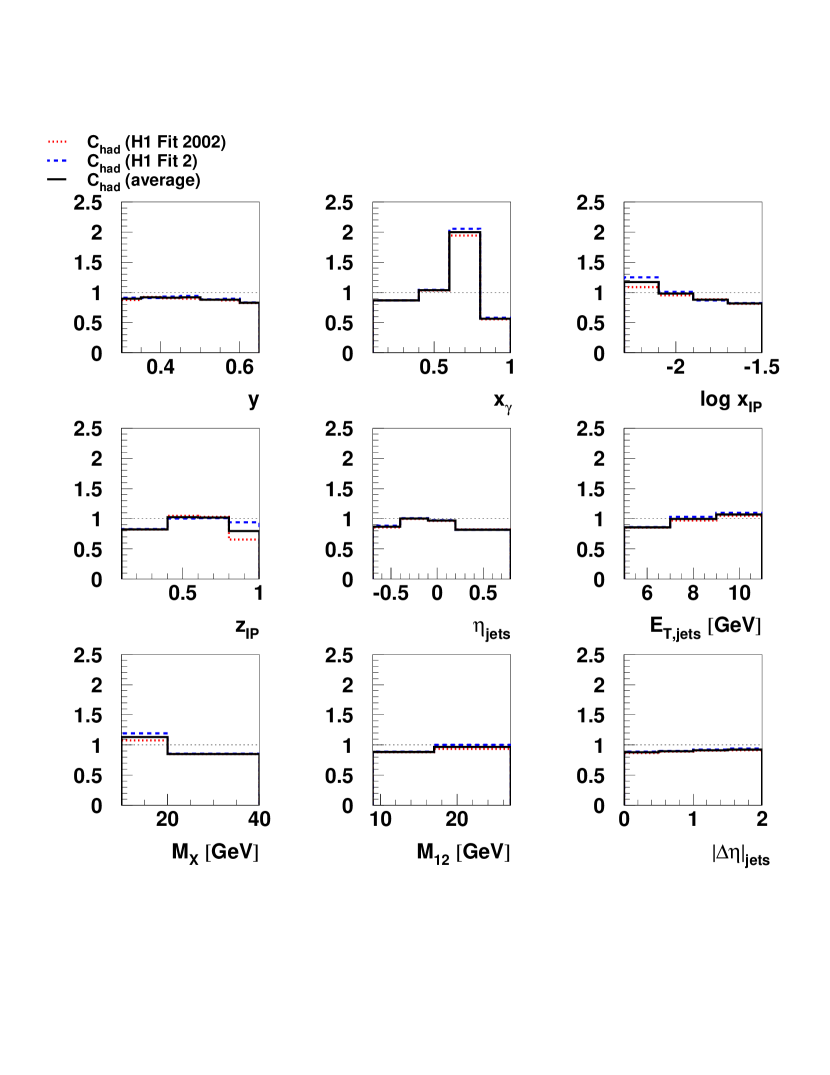
Figure 2: Ratios of hadronic to partonic dijet cross sections for two different fits of the parton densities in the pomeron H1 ; H11 as well as their average Schi .

Here, $C_{\rm had}$ is the ratio of the respective cross sections for hadronic jets to partonic jets. The correction factors have been calculated from Monte Carlo models including LO cross sections together with parton showering and subsequent hadronization by the H1 group Schi . As seen in Fig. 2, $C_{\rm had}$ is approximately equal to one with deviations less than $20\%$. The only exception is $C_{\rm had}$ for the $x_{\gamma}^{\rm jets}$ cross section with a value that is appreciably different from one for $x_{\gamma}^{\rm jets}\geq 0.6$.

The differential cross sections have been calculated in LO and NLO with varying scales, where the renormalization scale and both factorization scales are set equal and are $\mu=\xi E_{T}^{\rm jet1}$ with $\xi$ varied in the range $0.5\leq\xi\leq 2$. This way we hope to have a reasonable estimate of the error for the theoretical cross sections and are not in danger to base our conclusions concerning factorization breaking only on one particular scale choice. Note that for the pomeron PDFs the variation of the factorization scale is restricted by their parameterization to $M_{I\!\!P}^{2}\leq 150$ GeV².

The theoretical cross sections are presented in two versions in LO and NLO, respectively. In the first version no suppression factor $R$ is applied. It corresponds to the LO or NLO prediction with no factorization breaking, labeled $R=1$ in the figures. The second version is with a suppression factor $R=0.34$ in the resolved cross section, labelled $R=0.34$ in the figures. This particular value for $R$ is motivated by the recent work of Kaidalov et al. KKMR . These authors studied the ratio of diffractive to inclusive dijet photoproduction in the HERA regime with and without including unitarity effects, which are responsible for factorization breaking, as a function of $x_{\gamma}$. In this study they applied a very simplified dijet production model for this ratio, which is very similar to the model proposed by the CDF collaboration for $p\bar{p}$ collisions CDF . From the calculations of this ratio, with and without unitarity corrections, they obtained the suppression factor $R=0.34$ for $x_{\gamma}\leq 0.3$ (see Fig. 6 in Ref. KKMR ), which they attribute to the resolved part of the photoproduction cross section. We shall use this value of the suppression factor as a first try and apply it to the total resolved part in the LO calculation and to its NLO correction. The direct part is, in both cases, left unsuppressed ($R=1$). It is clear that not all of the distributions will be sensitive to the value of $R$. Furthermore, most of the distributions are normalized to one, so that the absolute magnitude can not be used as a discriminator for the occurence of a suppression factor.

Our LO (top) and NLO (bottom) results are shown in Fig. 3 for

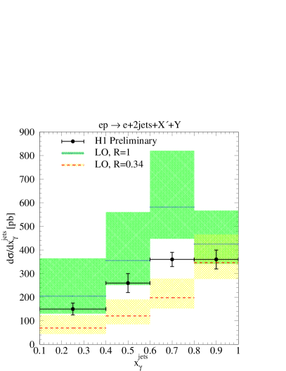
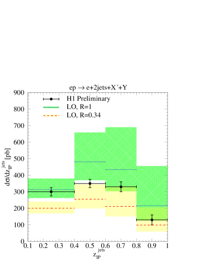
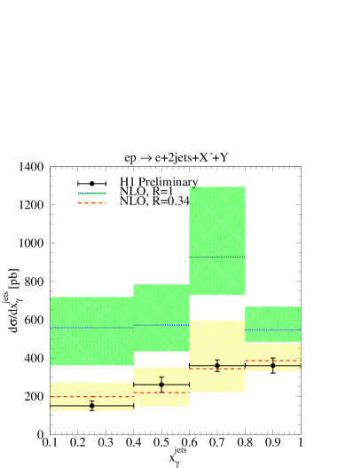
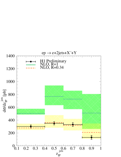
Figure 3: LO (upper) and NLO (lower) cross sections for diffractive dijet photoproduction as functions of $x_{\gamma}^{\rm jets}$ (left) and $z_{I\!\!P}^{\rm jets}$ (right), compared to preliminary H1 data. The shaded areas indicate a variation of scales by a factor of two around $E_{T}^{\rm jet1}$.

the differential cross sections in $x_{\gamma}^{\rm jets}$ (left) and $z_{I\!\!P}^{\rm jets}$ (right), which are not normalized to one. The normalized distributions in $x_{\gamma}^{\rm jets}$, $z_{I\!\!P}^{\rm jets}$, $\log_{10}x_{I\!\!P}$, $y$, $E_{T}^{\rm jet1}$, $M_{X}^{\rm jets}$, $M_{12}^{\rm jets},\overline{\eta}^{\rm jets}$, and $|\Delta\eta^{\rm jets}|$ are shown in LO and NLO in Figs. 4-8.

For $d\sigma/dx_{\gamma}^{\rm jets}$ (Fig. 3, left), we have very different cross sections for $R=1$ and $R=0.34$ and for the scale choice $\xi=1$. An exception is the highest $x_{\gamma}^{\rm jets}$-bin, where the difference is only $20\%$, since in this bin the direct contribution is dominant and the suppression factor is therefore less effective. In all the other bins, $d\sigma/dx_{\gamma}^{\rm jets}$ with $R=0.34$ is reduced by this factor as expected. Except for the highest $x_{\gamma}^{\rm jets}$-bin, neither of the two LO calculations agrees with the data. The $R=1$ cross section is too large and the $R=0.34$ cross section is too small. Only when we consider the scale variation with $0.5\leq\xi\leq 2$ as a realistic error estimate, we would conclude that the unsuppressed LO cross section ($R=1$) is marginally consistent with the H1 data inside the experimental errors. At NLO, the conclusion is reversed: the suppressed cross section now agrees very well with the data, while the unsuppressed cross section drastically overestimates the data.

For $d\sigma/dz_{I\!\!P}^{\rm jets}$ in Fig. 3 (right), the agreement of unsuppressed and suppressed cross sections with the data is equally marginal at LO, even within the respective error bands, while it is excellent for the suppressed NLO cross section. We remark that the suppressed and unsuppressed cross sections with $\xi=1$ differ approximately only by a factor 0.5, since in this distribution the direct and resolved contributione are superimposed differently than in $d\sigma/dx_{\gamma}^{\rm jets}$.

For the normalized $x_{\gamma}^{\rm jets}$ distributions in Fig. 4

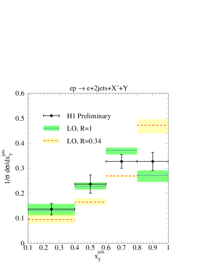
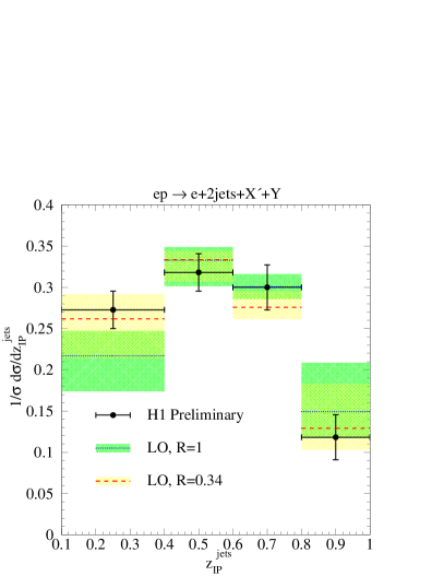
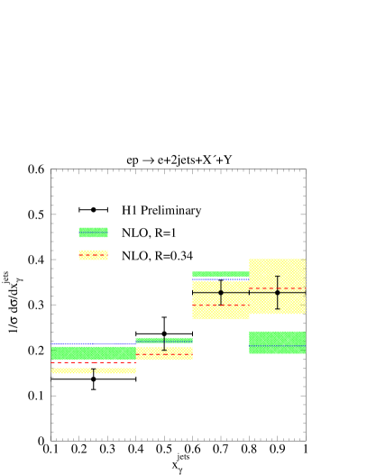
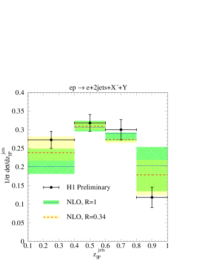
Figure 4: Normalized $x_{\gamma}^{\rm jets}$ (left) and $z_{I\!\!P}^{\rm jets}$ (right) distributions in LO (top) and NLO (bottom), compared to preliminary H1 data.

(left), the overall agreement is, of course, better. In particular, the unsuppressed LO distribution agrees now with the data within the scale uncertainty, whereas at NLO it is again the suppressed distribution that describes the data best. Furthermore, the scale uncertainty is substantially reduced in the normalized distributions as expected. For the $z_{I\!\!P}^{\rm jets}$ distributions in Fig. 4 (right), both the unsuppressed and suppressed LO distributions agree with the data within errors, while at NLO agreement is only found for the latter.

The comparison of the normalized distributions in $\log_{10}$ $x_{I\!\!P}$ and $y$ is shown in Fig. 5. Here the theoretical predictions for

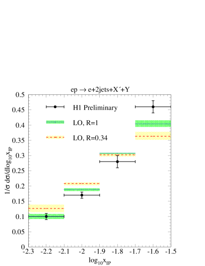
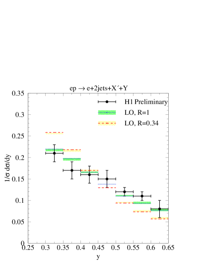
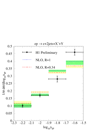
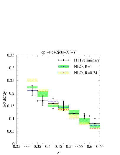
Figure 5: Normalized $\log_{10}x_{I\!\!P}$ (left) and $y$ (right) distributions in LO (top) and NLO (bottom), compared to preliminary H1 data.

$R=0.34$ and $R=1$ differ very little. This is understandable, since the $x_{I\!\!P}$ and $y$ dependence of the cross section factorize (see Eq. (13)) to a large extent. Only through the correlations due to the kinematical constraints we observe small differences between the $R=0.34$ and the $R=1$ cross sections, particularly in the $y$ distribution. From this comparison no definite conclusions concerning the suppression can be drawn. All theoretical predictions agree more or less with the data. In the highest $\log_{10}x_{I\!\!P}$ bin the measured point lies higher than the theoretical points. This can be explained, at least partly, by an additional sub-leading Reggeon contribution, which has not been taken into account in the diffractive PDFs we are using (see Fig. 7 in H13 ).

Next we look at the $E_{T}^{\rm jet1}$ distribution in Fig. 6. The

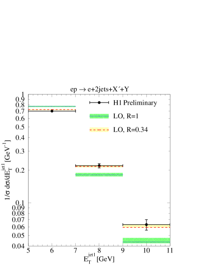
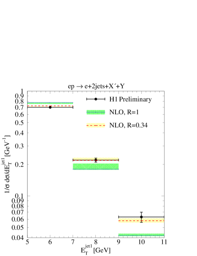
Figure 6: Normalized $E_{T}^{\rm jet1}$ distribution in LO (left) and NLO (right), compared to preliminary H1 data.

LO (left) and NLO (right) distributions with $R=0.34$ are flatter than the unsuppressed distribution as we expect it, since the resolved component occurs dominantly at the smaller $E_{T}^{\rm jet1}$. The suppressed cross section agrees better with the data points, even if the scale uncertainty is taken into account. Due to the normalization of the cross section, the differences between LO and NLO are almost invisible.

The distributions $1/\sigma~{}d\sigma/dM_{X}^{\rm jets}$ and $1/\sigma~{}d\sigma/dM_{12}^{\rm jets}$ are correlated due to $M_{X}^{\rm jets}=M_{12}^{\rm jets}/\sqrt{z_{I\!\!P}^{\rm jets}x_{\gamma}^{\rm jets}}$. Although the distributions in $x_{\gamma}^{\rm jets}$ and $z_{I\!\!P}^{\rm jets}$ are bound to reveal more detailed information on possible factorization breaking, we have calculated the mass distributions nevertheless. The results and the comparisons with the data are shown in Fig. 7. The

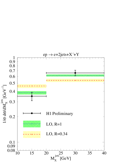
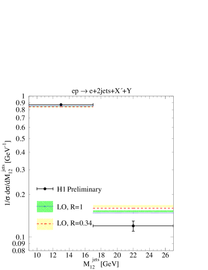
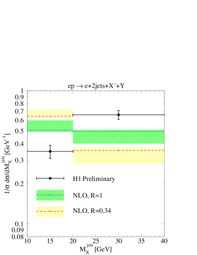
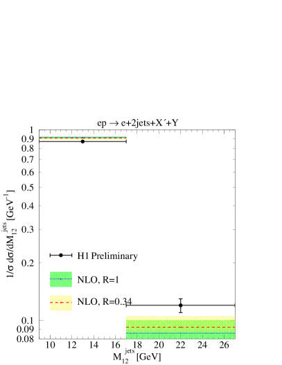
Figure 7: Normalized $M_{X}^{\rm jets}$ (left) and $M_{12}^{\rm jets}$ (right) distributions in LO (top) and NLO (bottom), compared to preliminary H1 data.

experimental cross sections increase with $M_{X}^{\rm jets}$, while they decrease with increasing $M_{12}^{\rm jets}$. This is due to the correlation mentioned above. The distribution in $M_{12}^{\rm jets}$ is also correlated with the distribution in $E_{T}^{\rm jet1}$. For the mass distribution of the dijet final state, which can directly be measured experimentally, the LO and NLO, suppressed and unsuppressed distributions are very similar and agree with the data. In contrast, the hadronic mass $M_{X}^{\rm jets}$ has to be reconstructed and is very sensitive to systematic errors in the measured variables. The theoretical prediction follows the increase in the data only in LO, while at NLO the dependency is reversed and is very sensitive to the presence of a possible third parton in the final state $X$.

The distributions in $\overline{\eta}^{\rm jets}$ and $|\Delta\eta^{\rm jets}|$ presented in Fig. 8 involve a delicate superposition of

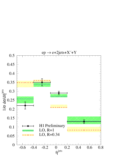
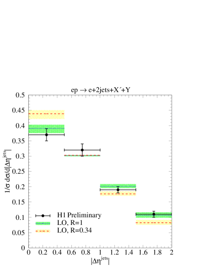
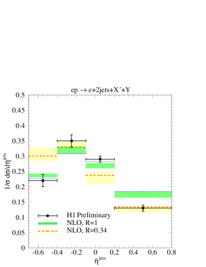
Figure 8: Normalized $\overline{\eta}^{\rm jets}$ (left) and $|\Delta\eta^{\rm jets}|$ (right) distributions in LO (top) and NLO (bottom), compared to preliminary H1 data.

direct and resolved contributions. In particular, the direct (resolved) process dominates for negative (positive) $\overline{\eta}$. While the LO $\overline{\eta}$-distribution agrees better with the data, if the resolved process is not suppressed ($R=1$), the conclusion is again reversed at NLO, as was already the case for the $x_{\gamma}^{\rm jets}$-distribution in Fig. 3. For the lowest bin in $\overline{\eta}$, we observe an excess of the theoretical prediction over the data, which is well known from studies of inclusive jet production at the very low transverse momenta studied here and which can be related to additional hadronization effects. The distribution in $|\Delta\eta^{\rm jets}|$ is intimately linked to the angular distribution of the partonic scattering matrix elements. It is thus less sensitive to the superposition of direct and resolved photon contributions, and the theoretical predictions agree almost equally well.

In summary, we conclude that for most LO distributions the unsuppressed theory, i.e. with no factorization breaking, agrees better with the experimental data. This conclusion is, however, premature, since at NLO it is the suppressed theory, i.e. with factorization breaking and $R=0.34$, which is preferred.

In KKMR , the suppression factor of $R=0.34$ was deduced from a calculation of the ratio of diffractive and inclusive dijet photoproduction at HERA as a function of $x_{\gamma}$ for two cases: (i) no absorption and (ii) absorption included. The calculation of this ratio for the two cases was based on a very simplified model, in which the ratio depended only on the gluon PDFs of the pomeron and proton in the numerator and denominator, respectively. It is of interest to see how this ratio behaves as a function of $x_{\gamma}^{\rm jets}$ for the two cases $R=1$ and $R=0.34$ in LO and NLO in the more detailed theory presented in this work, i.e. in a theory where this ratio is calculated from the full cross section formula in Eq. (13) and the corresponding formula for the inclusive dijet cross section with quarks and gluons and realistic experimental cuts.

The result is shown in Fig. 9 (left), where we have used the

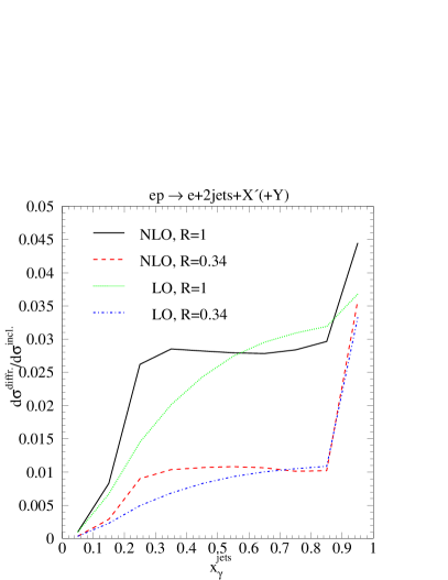
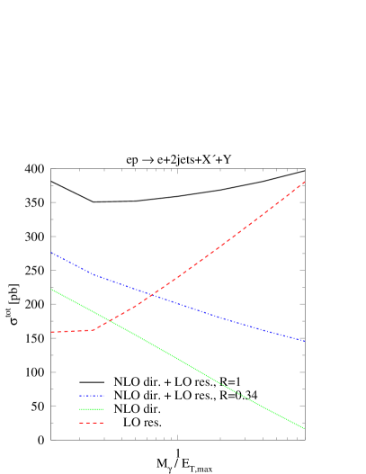
Figure 9: Ratio of diffractive to inclusive dijet photoproduction as a function of $x_{\gamma}^{\rm jets}$ (left) and photon factorization scale dependence of resolved and direct contributions together with their weighted sums (right).

CTEQ5M1 parameterization for the proton PDFs CTEQ in the inclusive cross section results. In LO and for $R=1$, the ratio $d\sigma^{\rm diffr}/d\sigma^{\rm incl}$ starts at small $x_{\gamma}^{\rm jets}=0.05$ at a very low value ($\simeq 0.001$) and then rises monotonically up to $0.032$ and $0.037$ at $x_{\gamma}^{\rm jets}=0.85$ and $0.95$. With $R=0.34$, i.e. with suppression of the resolved part, the increase of this ratio is very much reduced. It goes up to $0.011$ at $x_{\gamma}^{\rm jets}=0.85$. At $x_{\gamma}^{\rm jets}=0.95$ the ratio is substantially larger, since in this region the unsuppressed direct cross section dominates. We see that up to $x_{\gamma}^{\rm jets}=0.85$ the suppressed ratio ($R=0.34$) is reduced approximately by a factor of three as compared to the unsuppressed ratio ($R=1$) as expected. The behavior of the ratio is somewhat different for the NLO case. In particular, the diffractive NLO resolved contribution has a steeper rise at $x_{\gamma}^{\rm jets}=0.25$ and flatter behavior above, which is reflected in both the unsuppressed and the suppressed sum. Compared to the corresponding curves for $d\sigma^{\rm diffr}/d\sigma^{\rm incl}$ in KKMR , the qualitative behavior of our curves, in LO and NLO, is similar. The ’no absorption/absorption included’ curves in KKMR resemble more our LO than our NLO results as expected. We have to keep in mind, however, that the kinematic constraints applied in KKMR differ from ours, which are the same as in the experimental analysis. This translates mainly into a different (smaller) normalization of our results. Clearly it would be interesting to measure $d\sigma^{\rm diffr}/d\sigma^{\rm incl}$ as a function of $x_{\gamma}^{\rm jets}$ in order to have another observable for measuring the suppression as a function of $x_{\gamma}^{\rm jets}$. Compared to the cross section $d\sigma/dx_{\gamma}^{\rm jets}$ considered earlier, this ratio has the advantage to depend less on the photon PDFs, which appear both in the numerator and the denominator and should cancel to a large extent.

It may well be that our procedure to describe the factorization breaking by applying a suppression factor to the total resolved cross section is not correct and must be modified. An indication for this is the fact that the separation between the direct and the resolved process is not physical. It depends in NLO on the factorization scheme and scale $M_{\gamma}$, as already mentioned earlier. The sum of both cross sections is the only physically relevant cross section, which is approximately independent of the factorization scale $M_{\gamma}$. By multiplying the resolved part with the suppression factor $R=0.34$ the correlation of the $M_{\gamma}$-dependence between the direct and the resolved part is changed and the sum of both parts has a much stronger $M_{\gamma}$ dependence than for the unsuppressed case ($R=1$). This is shown in Fig. 9 (right). We see the compensation of the $M_{\gamma}$-dependence between the NLO direct cross section (dotted line) and the LO resolved cross section (dashed line) in the unsuppressed ($R=1$) case, leading to a fairly $M_{\gamma}$ independent sum of both contributions (full line) KKK ; BKS . When the LO resolved part is suppressed with the factor $R=0.34$, the compensation is reduced, and the sum of the NLO direct and LO resolved parts becomes much more $M_{\gamma}$-dependent than before (although not too much in the range $0.5<M_{\gamma}/E_{T,\max}<2$, as seen by the dashed-dotted curve in the right part of Fig. 9).

The compensation of the $M_{\gamma}$-dependence between the NLO direct and LO resolved cross section occurs via the anomalous or point-like part of the photon PDFs. This means that this part of the PDFs is closely related to the direct cross section. It is usually assumed that the direct part obeys factorization and has no suppression factor. So the point-like part in the photon PDFs should not be suppressed either, and the suppression factor should be applied only to the hadron-like part and the gluon part of the photon PDFs. Since all three parts, point-like, hadron-like and gluon, are correlated through the evolution equations, it is not clear how this suggestion could be realized. Of course, if the point-like part is not suppressed, the problem of the insufficient compensation of the scale dependence of the NLO direct and LO resolved part would be solved. It is, however, conceivable that this problem would be solved quite naturally if one attempts to incorporate absorptive effects into the NLO theory following, for example, the work of Kaidalov:2001iz .

4 Conclusions and Outlook

The recent measurement of diffractive dijet photoproduction combined with the analysis of diffractive inclusive DIS data in terms of diffractive PDFs offers the opportunity to test factorization in diffractive dijet photoproduction. For this purpose we have calculated several cross sections and normalized distributions for various kinematical variables in LO and NLO and compared them with recent preliminary H1 measurements H13 . In LO we found that the measured distributions und unnormalized cross sections agree quite well with the theoretical results if, by a reasonable variation of scales, a theoretical error is taken into account. This means that in a LO comparison there is no evidence for a possible factorization breaking expected for the resolved contribution. However, it is well known that for dijet photoproduction NLO corrections are very important for the direct and in particular for the resolved contributions to the cross section. Indeed, the theoretical results at NLO disagree with the data for unnormalized cross sections like $d\sigma/dx_{\gamma}^{\rm jets}$ and $d\sigma/dz_{I\!\!P}^{\rm jets}$. Agreement between data and theoretical results is found, however, if the resolved contribution is suppressed by a factor $R=0.34$. This factor is motivated by a recent calculation of absorptive effects in diffractive dijet photoproduction KKMR . Since NLO results are more trustworthy than any LO cross section calculations, we consider our findings a strong indication that factorization breaking occurs in diffractive dijet photoproduction with a rate of suppression expected from theoretical models.

It would be interesting to investigate hard diffractive photoproduction of other final states, for which the superposition of direct and resolved contributions is different. Such diffractive photoproduction reactions are, e.g., large-$p_{T}$ inclusive single-hadron production, heavy-flavour production with or without jets, and prompt photon production. In order to verify that factorization breaking disappears when the $Q^{2}$ of the virtual photon is increased from small to larger values, it would be desirable to have measurements of diffractive production of the final states mentioned above as a function of $Q^{2}$.

Finally factorization breaking is expected not only in the diffractive region, $x_{I\!\!P}\ll 1$, but also at larger values of $x_{I\!\!P}$ where Regge exchanges other than the pomeron occur. For example, pion exchange is strong in all reactions with a leading neutron. Here, dijet photoproduction with a leading neutron has been studied in LO and NLO KKn and compared to ZEUS experimental data Zeusn . This process could also be a candidate for factorization breaking in the resolved contribution.

- (1) H1 Collaboration, paper 980 submitted to the 31st Int.’l Conf. on High Energy Physics ICHEP 2002, Amsterdam, and paper 089 submitted to the EPS 2003 Conf., Aachen.
- (2) J. Collins, Phys. Rev. D 57 (1998) 3051, Phys. Ref. D 61 (2000) 019902 (E), and J. Phys. G 28 (2002) 1069.
- (3) CDF Collaboration, T. Affolder et al., Phys. Rev. Lett. 84 (2000) 5043.
- (4) H1 Collaboration, C. Adloff et al., Z. Phys. C 76 (1997) 613.
- (5) L. Alvero et al., Phys. Rev. D 59 (1999) 074022.
- (6) A.B. Kaidalov, V.A. Khoze, A.D. Martin, and M.G. Ryskin, Eur. Phys. J. C 21 (2001) 521 and references therein.
- (7) M. Klasen and G. Kramer, Z. Phys. C 72 (1996) 107 and 76 (1997) 67; M. Klasen, T. Kleinwort, and G. Kramer, Eur. Phys. J. Direct C 1 (1998) 1.
- (8) S. Frixione and G. Ridolfi, Nucl. Phys. B 507 (1997) 315.
- (9) H1 Collaboration, C. Adloff et al., Report DESY 02-225, February 2003, submitted to Eur. Phys. J. C and earlier H1 papers given there.
- (10) ZEUS Collaboration, S. Chekanov et al., Eur. Phys. J. C 23 (2002) 615, Phys. Lett. B 531 (2002) 9, Phys. Lett. B 560 (2003) 7, and earlier ZEUS papers given in these references.
- (11) M. Klasen, Rev. Mod. Phys. 74 (2002) 1221.
- (12) H1 Collaboration, paper 987 submitted to the 31st Int.’l Conf. on High Energy Physics, ICHEP 2002, Amsterdam, and paper 087 submitted to the EPS 2003 Conf., Aachen.
- (13) S. Ellis and D. Soper, Phys. Rev. D 48 (1993) 3160; S. Catani et al., Nucl. Phys. B 406 (1993) 187.
- (14) M. Klasen and G. Kramer, Phys. Lett. B 366 (1996) 385; S. Frixione and G. Ridolfi, Nucl. Phys. B 507 (1997) 315.
- (15) G. Ingelman and P. Schlein, Phys. Lett. B 152 (1985) 256.
- (16) S. Frixione et al., Phys. Lett. B 319 (1993) 339.
- (17) D. Bödeker, G. Kramer, and S.G. Salesch, Z. Phys. C 63 (1994) 471.
- (18) M. Glück, E. Reya, and A. Vogt, Phys. Rev. D 45 (1992) 3986 and D 46 (1992) 1973.
- (19) F.-P. Schilling, private communication.
- (20) A.B. Kaidalov, V.A. Khoze, A.D. Martin, and M.G. Ryskin, Phys. Lett. B 567 (2003) 61.
- (21) CTEQ Collaboration, H.L. Lai et al., Eur. Phys. J. C 12 (2000) 375.
- (22) M. Klasen and G. Kramer, Phys. Lett. B 508 (2001) 259; M. Klasen, J. Phys. G 28 (2002) 1091.
- (23) ZEUS Collaboration, J. Breitweg et al., Nucl. Phys. B 596 (2001) 3.