Exact identification of the radion and its coupling to the observable sector

Abstract

Braneworld models in extra dimensions can be tested in laboratory by the coupling of the radion to the Standard Model fields. The identification of the radion as a canonically normalized field involves a careful General Relativity treatment: if a bulk scalar is responsible for the stabilization of the system, its fluctuations are entangled with the perturbations of the metric and they also have to be taken into account (similarly to the well-developed theory of scalar metric perturbations in $4$D cosmology with a scalar field). Extracting a proper dynamical variable in a warped geometry/scalar setting is a nontrivial task, performed so far only in the limit of negligible backreaction of the scalar field on the background geometry. We perform the general calculation, diagonalizing the action up to second order in the perturbations and identifying the physical eigenmodes of the system for any amplitude of the bulk scalar. This computation allows us to derive a very simple expression for the exact coupling of the eigenmodes to the Standard Model fields on the brane, valid for an arbitrary background configuration. As an application, we discuss the Goldberger-Wise mechanism for the stabilization of the radion in the Randall-Sundrum type models. The existing studies, limited to small amplitude of the bulk scalar field, are characterized by a radion mass which is significantly below the physical scale at the observable brane. We extend them beyond the small backreaction regime. For intermediate amplitudes, the radion mass approaches the electroweak scale, while its coupling to the observable brane remains nearly constant. At very high amplitudes, the radion mass instead decreases, while the coupling sharply increases. Severe experimental constraints are expected in this regime.

I Introduction

Braneworlds embedded in higher dimensions have opened new interesting directions in high energy particle physics, general relativity, and cosmology. The Randall-Sundrum (RS) model with warped $5$D bulk geometry between two plane-parallel orbifold branes RS1 has been particularly studied. Its low energy spectrum contains a scalar field, denoted as radion $Q$, which is associated to the inter-brane modulus. The radion is coupled to Standard Model (SM) fields living on one brane, which gives very interesting phenomenology for accelerator experiments phenomenology . The coupling is of the form

$${\cal L}_{int}=\frac{Q}{\Lambda}\,T^{\mu}_{\mu}\,,$$ (1)

where $T^{\mu}_{\mu}$ is the trace of the energy momentum of the SM fields, $Q$ refers to the radion field, while the coupling $\Lambda$ is close to the electroweak scale GW ; GW2 ; csaki1 ; csaki2 .

The radion originates from the scalar fluctuations of the bulk geometry. In the RS model RS1 the two branes are at indifferent equilibrium: the interbrane distance is a free parameter, corresponding to a massless radion. The situation is changed if a bulk scalar field $\phi$ is introduced to stabilize the system, as in the Goldberger-Wise mechanism GW . The identification and the study of the properties of the radion field are less straightforward in this case. The initial studies, including the original work GW , were based on the effective $4$D theory, obtained integrating an approximate ansatz for the geometry and the scalar field profile along the extra coordinate. However, the introduction of the bulk scalar makes the gravity/scalar system more complex, and requires a self-consistent treatment based on the $5$D Einstein eqs. Dewolfe ; GR . In particular, the scalar fluctuations $\Phi$ of the bulk metric are sourced by the fluctuations $\delta\phi$ of the bulk scalar field, and the coupled linearized system $\left(\Phi,\delta\phi\right)$ also has to be treated self-consistently. The $5$ dimensional equations for the system were derived in the basic papers Tanaka:2000er ; csaki2 . The analysis of csaki2 is particularly advanced and clear with respect to the coupling of the modes, so we will often refer to it for comparison. The properties of the radion obtained in these studies are nonetheless in good agreement with the ones from the $4$D effective theory (the agreement is actually much better than what has been claimed sometimes in the literature, as we will discuss below).

All the existing studies share one limitation: it is always assumed that the bulk scalar field has a negligible backreaction on the background geometry (the only effect being that it lifts up the flat direction corresponding to the radion). Phenomenological studies have so far been restricted to this case, first because it is only in this limit that the bulk geometry is (approximately) AdS as in the RS proposal, but also because it is the only case for which the properties of the radion were known. Indeed, in this limit the contribution of $\delta\phi$ to the wave function of the radion is negligible, and the radion behaves approximately like the metric perturbation $\Phi\,$ csaki2 . As a consequence, the exact diagonalization of the coupled $\left(\Phi,\delta\phi\right)$ system in not required in this limit.

In contrast to these works, the aim of the present paper is to study the scalar perturbations for the general situation in which the bulk scalar $\phi$ has arbitrary amplitude. The main motivation is that very small $\phi$ should not be considered as completely natural, since the idea of RS is to avoid strong hierarchies besides the one given by the warp factor.  There is no incompatibility between a sizable $\phi$ and the main idea of RS1 : although the bulk geometry will be in general different from pure AdS, one can still naturally achieve a strong warping at the observable brane, as needed to solve the hierarchy problem. In particular, this is also true for the Goldberger-Wise mechanism GW and its generalizations. The main obstacle is that the mixing between the different scalar perturbations cannot any longer be neglected, and the coupled system of perturbations has to be diagonalized. This study is still missing in the existing literature, and it is the main result of the present work. As we will show, the coupled $\left(\Phi,\delta\phi\right)$ pair contains a single dynamical variable which we denote by $v$, and which is a linear superposition of the pair. The equation for $v$ reduces to an oscillator-like equation. More importantly, the action of the system can be shown to be diagonal in terms of the $4$D Kaluza-Klein modes of $v\,$, which we denote by $Q_{n}\,$. In this way, we obtain the exact $4$D action for the physical scalar modes of the theory. The action differs from the effective (approximate) $4$D theory which has been computed in the literature by neglecting the $\delta\phi$ modes, and - moreover in general - by starting from a $5$D ansatz which does not satisfy the linearized equations for the perturbations (the effective action is derived and discussed in Appendix C, to emphasize the difference from the exact $4$D theory discussed in the rest of the paper).

The final result can be easily summarized. Decomposing the metric perturbation in terms of the $4$D KK modes, $\Phi=\sum_{n}{\tilde{\Phi}_{n}}\left(y\right)\,Q_{n}\left(x\right)$ ($y$ denoting the extra coordinate), we find that the quadratic action for the scalar modes can be cast in the diagonal form

$$S=\sum_{n}S_{n}=\sum_{n}C_{n}\int d^{4}x\;Q_{n}\left[\,\Box-m_{n}^{2}\,\right]Q_{n}\,\,,$$ (2)

where $m_{n}^{2}$ are the physical masses obtained from an eigenvalue boundary problem in the extra dimension (see below). As we remarked, the radion corresponds to the mode with the lowest mass. The fields $Q_{n}$ are scalars fields of the exact $4$D theory, and their decoupled actions can be trivially quantized. The coefficients $C_{n}$ are given by

$$C_{n}=\frac{3\,M^{3}}{2}\int_{0}^{y_{0}}\frac{dy}{A}\,\left[\frac{3\,M^{3}}{2\,\phi^{\prime\,2}}\,\left(A^{2}\,{\tilde{\Phi}}_{n}\right)^{\prime\,2}\,+\left(A^{2}\,{\tilde{\Phi}}_{n}\right)^{2}\right]\,\,.$$ (3)

In this expression, $A$ is the warp factor, $M$ the fundamental scale of gravity in $5$ dimensions, and prime denotes differentiation with respect to $y\,$. This result is particularly simple and completely general, since it holds for arbitrary background configurations $A$ and $\phi\,$. The derivation, to be discussed in detail below, exploits the strong similarity of the system with the one of scalar metric fluctuations in the scalar field inflationary cosmology. This analogy allows us to identify the dynamical variable $v$, which in inflationary cosmology is known as the Mukhanov-Sasaki variable mukhanov ; sasaki , and which is the starting point of our computation.

The requirement that the modes $Q_{n}$ are canonically normalized, $C_{n}\equiv 1/2\,$, fixes the normalization of ${\tilde{\Phi}}_{n}\,$, which in turn defines the strength of the coupling of the radion and of the other KK modes to the SM fields on the observable brane (the computation and diagonalization of the action is indeed necessary for this task. The normalization of the modes cannot be derived from the Einstein equations for the perturbations, which are all linear in the perturbations). Similarly to the initial expression (1), the coupling $\Lambda_{n}$ of the radion and the other KK modes to brane fields is given by

$${\cal L}_{{\rm int},n}=\frac{Q_{n}}{\Lambda_{n}}\,T^{\mu}_{\mu}\quad\quad,\quad\quad\Big{|}\frac{1}{\Lambda_{n}}\Big{|}=\Big{|}\frac{{\tilde{\Phi}}_{n}\left(y_{0}\right)}{2}\Big{|}\,\,.$$ (4)

where $y_{0}$ is the location of the observable brane. Due to the explicit knowledge of (3), we can determine the coupling of all the perturbations for arbitrary background configuration. Our general calculation confirms the accuracy of the results of csaki2 in the limit of small $\phi\,$.  Our results extend these calculations to a general amplitude of the field $\phi$ and to an arbitrary geometry $A\,$.

The paper is organized as follows. In section II we present the action and the relevant equations of the system. The main result summarized above is derived in section III, while it is applied to a couple of specific examples in section IV, one of which - first proposed in Dewolfe - is a generalization of the Goldberger-Wise mechanism GW for the stabilization of the radion of the Randall-Sundrum model RS1 . The existing studies of the phenomenology of this model, limited to small amplitude of the bulk scalar field, are characterized by a radion mass which is significantly below the physical scale at the observable brane. This hierarchy decreases as $\phi$ increases, and, fore sizable values of $\phi\,$, the radion mass approaches the electroweak scale. On the contrary, the coupling of the radion to the observable sector remains constant for a wide range of $\phi\,$. The radion mass reaches a maximal value for a finite value of $\phi\,$. At higher amplitudes the mass decreases, while its coupling to the SM sharply increases. In section V we verify numerically some of these analytical results: we follow the oscillations of a two-brane system around a static configuration with the numerical code developed in bc ; the frequency spectrum of the oscillations exhibits resonances precisely in correspondence to the masses of the modes given by the analytical computation. The higher resonances are excited by the their coupling to the radion in the nonlinear regime. Once their amplitude becomes small, they become constant in time, confirming the fact that they are decoupled at the linear level. The results of the paper are discussed in section VI, where we also comment on more general related issues. For example, we discuss preheating effects due to the oscillations of the radion, and the linearized $4$D gravity on the branes. The paper is concluded by three Appendices. In the first one we compute the quadratic action for the perturbations. Appendix B presents analytical results in the small $\phi$ limit. Finally, Appendix C contains the computation of the effective $4$D action for the radion, and the comparison with the exact results discussed in the rest of the paper.

II Set-up

We start from the action

$$S=2\int_{0}^{y_{0}}d^{5}x\sqrt{-g}\left[\frac{M^{3}}{2}R-\frac{1}{2}\left(\partial\,\varphi\right)^{2}-V\left(\varphi\right)\right]-\sum_{i=1,2}\int d^{4}x\sqrt{-\gamma}\left\{2M^{3}\left[K\right]+U\left(\varphi\right)\right\}\,\,,$$ (5)

where the first term is the bulk action, and the sum contains contributions from the two branes, located at $y=0$ and $y=y_{0}\equiv-y_{0}$ along the extra dimension. The overall factor of $2$ multiplying the first term accounts for the integration over the intervals $[-y_{0},0]$ and $[0,y_{0}]$, which are identified by an $S^{1}/{\mathbb{Z}}_{2}$ symmetry. To shorten the notation, the bulk cosmological constant is included in the bulk potential $V\,$, while brane tensions are included in the brane potentials $U\,$. The quantity $\left[K\right]$ denotes the jump of the extrinsic curvature at the two branes, while $M$ is the fundamental scale of gravity in $5$ dimensions. We choose the following line element

$$ds^{2}=A\left(y\right)^{2}\left[\left(1+2\Psi\right)\eta_{\mu\nu}\,dx^{\mu}\,dx^{\nu}+\left(1+2\Phi\right)dy^{2}\right],$$ (6)

where Greek indices span the $1+3$ coordinates parallel to the flat branes, and $\eta={\rm diag}\left(-1,1,1,1\right)\,$. Namely, we have conformal coordinates for the warped background geometry, while the scalar metric perturbations $\Psi$ and $\Phi$ are expressed in the (generalized) longitudinal gauge.  Perturbations of the bulk scalar field are denoted $\varphi\left(x,y\right)=\phi\left(y\right)+\delta\phi\left(x,y\right)\,$. We are interested in static warped configurations (and, in addition, flat branes), so that the two background quantities $A$ and $\phi$ depend on the extra coordinate $y$ only. Concerning the background quantities, variation of the action (5) gives the bulk equations (here and in the following, prime denotes derivative wrt $y\,$)

$$\phi^{\prime\prime}+3\,\frac{A^{\prime}}{A}\,\phi^{\prime}-A^{2}\,V^{\prime}=0\,\,,$$

$$\frac{A^{\prime\prime}}{A}=2\frac{A^{\prime 2}}{A^{2}}-\frac{\phi^{\prime 2}}{3\,M^{3}}\,\,,$$

$$6M^{3}\frac{A^{\prime 2}}{A^{2}}=\frac{\phi^{\prime 2}}{2}-A^{2}\,V\,\,,$$ (7)

as well as the junction conditions

$$\frac{A^{\prime}}{A^{2}}=\mp\frac{U}{6\,M^{3}}\quad,\quad\quad\frac{\phi^{\prime}}{A}=\pm\frac{U^{\prime}}{2}\,\,,$$ (8)

where the upper and lower sign refers to the brane at $y=0$ and $y=y_{0}\,$, respectively (prime on the potentials $V$ and $U$ denotes differentiation with respect to $\phi\,$).

As with the background, not all of the equations for the perturbations are dynamical, reflecting the fact that not all the modes given above are physical. The system of linearized Einstein equations for the perturbations include the two constraint equations

$$\Phi-\frac{A}{A^{\prime}}\Psi^{\prime}-\frac{A\,\phi^{\prime}}{3\,M^{3}\,A^{\prime}}\,\delta\phi=0\,\,,$$

$$\Phi=-2\,\Psi\,\,.$$ (9)

as well as a dynamical equation. By using the constraint equations, the latter can be written as

$$\left[\Box+\frac{d^{2}}{d\,y^{2}}-\frac{\left(1/z\right)^{\prime\prime}}{1/z}\right]{\cal U}=0\,\,,$$ (10)

where we have defined

$$z\equiv\sqrt{2}\frac{A^{5/2}\,\phi^{\prime}}{A^{\prime}}\quad\quad,\quad\quad{\cal U}\equiv\frac{A^{3/2}}{\phi^{\prime}}\,\Psi\,\,,$$ (11)

and where $\Box$ is the D’Alambertian operator in $4$ d. Finally, there are two junction conditions for the perturbations at the two branes,

$$\left(A^{2}\,\Phi\right)^{\prime}=\frac{2\,A^{2}\,\phi^{\prime}\,\delta\phi}{3\,M^{3}}\,\,,$$

$$\delta\phi^{\prime}-\phi^{\prime}\,\Phi=\pm\frac{1}{2}\,A\,U^{\prime\prime}\,\delta\phi\,\,.$$ (12)

The first of these conditions could have also be obtained from the two constraint equations (9) evaluated at the two branes. The second condition instead contains additional, physically relevant information, relating $\delta\phi$ to the “mass parameters” of the scalar field at the two branes. As can be intuitively expected, very high $U^{\prime\prime}$ force $\delta\phi=0$ at the two branes. This is the case which is typically considered in the literature (starting from the original proposal GW ), since the results simplify significantly in this limit. In the next section we perform the identification and quantization of the perturbations for arbitrary $U^{\prime\prime}$, and we give general formulae valid for arbitrary bulk and brane potentials for $\phi\,$. The examples of section IV are instead restricted to high $U^{\prime\prime}\,$.

III Quantization of the action for perturbations and the identification of the physical modes.

From the analysis of the previous section, we see that scalar metric perturbations are coupled to the fluctuations of the bulk scalar field responsible for the stabilization of the system. The covariant formulation (5) fully underlines the symmetries of the theory. However - as in all gauge theories - the price to pay is the introduction of auxiliary degrees of freedom, so that it is not straightforward to identify and decouple the physical modes of the system. However, this is very important if we want to know their properties, namely their masses and their coupling to the (electroweak) sector on the observable brane. The mass spectrum for the perturbations can be obtained directly from the equations of motion. The easiest way to do so is to first identify some linear combination of the perturbations for which the dynamical equation can be cast in a Schrödinger-type form Tanaka:2000er ; csaki2 ; FK ; lorentzo . This is the case for the variable ${\cal U}$ defined in eq. (11), although other combinations can be used (see below). After solving this equation, the spectrum of the system can be obtained from the boundary conditions (12) at the two branes.

This procedure, however, does not identify which combination $v$ of the perturbations corresponds to the physical degrees of freedom, nor does it determine the proper normalization of the modes, since the bulk and boundary conditions are linear in the perturbations.  On the other hand, this information is needed to determine the coupling of the physical modes to the observable sector, see eq. (4). To obtain it, one has to diagonalize the action $S_{2}$ for these modes, which is computed by expanding the initial action (5) up to second order in the perturbations. This is a more difficult exercise than simply obtaining the equations of motion for the perturbations, and indeed it is the main original result of the present work.

We divide the discussion in two subsections. In the first one we quantize the system for the case in which the bulk scalar field $\phi$ is absent. This is a particularly simplified situation, since in this case there is only one physical scalar perturbation. This computation, which is the only one given in the literature, allows us to determine the normalization of the radion when the bulk scalar field is absent or when its backreaction on the bulk geometry can be neglected csaki2 . As shown in csaki2 , the contribution of $\delta\phi$ to the wave function of the radion is negligible in this limit, and the coupling of the radion to brane fields is (approximately) given by the coupling of $\Phi\,$. In subsection III.2 we perform the general calculation, valid for a bulk scalar field of any amplitude. This computation confirms the accuracy of the analysis of csaki2 in the limit in which the backreaction of $\phi$ is small and can be treated perturbatively. In addition, it gives new interesting results. First, as we mentioned, it provides the coupling of the radion to brane fields for arbitrary values of $\phi\,$. Second, it allows the computation of the coupling of the other KK modes, which cannot be approximated by the analysis of III.1 even in the small $\phi$ limit. The reason for this is the discontinuity in the number of modes with or without the bulk scalar field: when $\phi$ is absent, there is only one physical scalar degree of freedom (the radion). On the contrary, there is a whole tower of KK modes when the scalar field is present (no matter how small its amplitude is). Hence, the study of the action without $\phi$ does not provide any information about the KK modes.

III.1 Computation without the bulk scalar field

It is very instructive to study what happens when the scalar field is absent. Expanding the action (5) at quadratic order in the perturbations, and imposing $\Psi=-\Phi/2\,$, we find 

$$S_{2}\left[\varphi=0\right]= 2M^{3}\int d^{5}x\,A^{3}\left[\frac{-3}{4}\eta^{\mu\nu}\partial_{\mu}\Phi\partial_{\nu}\Phi+\frac{3}{2}\Phi^{\prime 2}+6\frac{A^{\prime}}{A}\Phi\Phi^{\prime}+\left(12\frac{A^{\prime 2}}{A^{2}}-3\frac{A^{\prime\prime}}{A}\right)\Phi^{2}\right]\,\,.$$ (13)

From eq. (9) we have

$$\Phi^{\prime}+2\frac{A^{\prime}}{A}\Phi=0\;\;\;\Rightarrow\;\;\;\Phi\propto A^{-2}\,\,.$$ (14)

Hence, in this case there is only one scalar eigenmode, corresponding to the radion field, while the tower of KK modes is absent cgr . We can then eliminate $\Phi^{\prime}$ in favor of $\Phi\,$, so that the action (13) becomes

$$S_{2}\left[\varphi=0\right]=2M^{3}\int d^{5}xA^{3}\left[-\frac{3}{4}\eta^{\mu\nu}\partial_{\mu}\Phi\partial_{\nu}\Phi+3\left(2\,\frac{A^{\prime 2}}{A^{2}}-\frac{A^{\prime\prime}}{A}\right)\Phi^{2}\right]\,\,.$$ (15)

The second term vanishes due to the background equations (7). We thus recover the well known result of a massless radion in the absence of any bulk field. Decomposing

$$\Phi\left({\bf x},y\right)={\tilde{\Phi}}\left(y\right)Q\left({\bf x}\right)\,\,,$$ (16)

the above action becomes

$$S=-\frac{3\,M^{3}}{2}\int_{0}^{y_{0}}dy\,A^{3}\,{\tilde{\Phi}}^{2}\int d^{4}x\eta^{\mu\nu}\partial_{\mu}Q\partial_{\nu}Q\equiv-\frac{1}{2}\int d^{4}x\,\eta^{\mu\nu}\,\partial_{\mu}Q\,\partial_{\nu}Q\,\,.$$ (17)

The last condition (i.e. the request that the $4$D field $Q$ is canonically normalized) specifies the normalization of ${\tilde{\Phi}}\,$, which in turns determines the coupling of the radion with the fields on the observable brane. The quantization of the last expression is straightforward.

When the bulk scalar is absent, the function $Q\,$, which encodes the physical degree of freedom, obeys the free wave equation $\Box Q=0\,$. The free bulk wave equation is satisfied by the bulk gravitational waves $h_{AB}$. The $5$ bulk degrees of freedom of $h_{AB}$ are projected to the $4$D brane as two tensor modes (corresponding to usual $4$D gravitons), two gravi-vectors (which are however absent at orbifold branes) and one gravi-scalar. When the bulk scalar is absent, we suggest interpreting the massless radion $Q$ as the massless gravi-scalar projection of the bulk graviton.

When the branes are stabilized by the bulk scalar field, the massless gravi-scalar projection is absent andrei . However, this degree of freedom does not disappear. The dynamical degree of freedom will be in this case a linear combination of the metric perturbation $\Phi$ and the fluctuation of the scalar field $\delta\phi\,$, and it emerges as a massive radion at the brane, rather than as a gravi-scalar (see the next section for details). The situation is similar to the re-shuffling of the degrees of freedom which occurs during a symmetry breaking, where here the symmetry breaking is associated with the stabilization of the interbrane distance.

III.2 General computation with a bulk scalar field

The expansion of the action (5) at second order in the perturbations gives

$$S_{2}=2M^{3}\!\!\int d^{5}x\,A^{3}\left\{\eta^{\mu\nu}\!\!\left[\frac{\partial_{\mu}\delta\phi\,\partial_{\nu}\delta\phi}{-\,2\ M^{3}}+3\partial_{\mu}\left(\Phi+\Psi\right)\partial_{\nu}\Psi\right]-\frac{1}{2\,M^{3}}\delta\phi^{\prime 2}+6\Psi^{\prime 2}+\frac{1}{M^{3}}\,\phi^{\prime}\delta\phi^{\prime}\left(\Phi-4\Psi\right)+\right.$$

$$\left.+12\frac{A^{\prime}}{A}\Psi^{\prime}\left(-\Phi+2\Psi\right)-\left(\frac{\phi^{\prime 2}}{M^{3}}-12\frac{A^{\prime 2}}{A^{2}}\right)\left(\frac{1}{2}\Phi^{2}+4\Psi^{2}\right)-\left[\frac{1}{2\,M^{3}}A^{2}V^{{}^{\prime\prime}}\delta\phi^{2}-\frac{1}{M^{3}}A^{2}V^{\prime}\delta\phi\left(\Phi+4\Psi\right)\right]\right\}+$$

$$-2\sum_{i}\int d^{4}xA^{4}\left[2U\Psi^{2}+2U^{\prime}\delta\phi\Psi+\frac{1}{4}U^{\prime\prime}\delta\phi^{2}\right]\,\,.$$ (18)

The derivation is given in Appendix A. Due to the presence of the bulk scalar field and its fluctuations, the general expression (18) is more involved than (13), and the quantization is more difficult. There are however similarities with the well known problem of scalar perturbations in $4$D inflationary cosmology with a scalar field, which fortunately can be exploited in the case at hand.  In the cosmological set-up, the inflaton field is the analogous of the bulk scalar $\phi\,$, and the time $t$ is analogous to the bulk coordinate $y\,$ (the scale factor $a\left(t\right)$ is the analogue of the warp factor $A\left(y\right)\,$). The evolution equations for the inflationary case constitute an initial value problem (initial conditions specified at some early time during inflation), which is in our case replaced by a boundary value problem (junction conditions at the two branes). The analogy cannot be pursued up to the quantization (in both cases, a canonical quantization is performed, and the $t\leftrightarrow y$ analogy has to be abandoned). However, it allows us to identify the dynamical variable $v$ which is the starting point for the quantization of (18). There are two complications compared to the inflationary case. The first is that, from the $4D$ point of view, the system (18) contains an infinite KK tower of scalar perturbations, while there is only one scalar mode in the inflationary case (as it was also the case in the previous subsection). The second is the presence of two branes as boundaries of the $y$ coordinate. Total derivatives in $y$ cannot be dropped (unlike the cosmological situation, where the space has no boundaries). As we shall see, they are actually crucial to ensure the orthogonality of the different modes in the action.

Starting from the action (18), we first eliminate $\Phi$ by use of the first of (9) (nondynamical equations, have to be used for the quantization. They compensate for the presence of non-physical degrees of freedom in the set of perturbations). We then identify total derivatives, and simplify the final expression by use of the background equations. Finally, we use $\Psi=-\Phi/2$ to express $\Psi$ (and its derivatives) back in terms of $\Phi\,$. Although the calculation is rather involved, the final result is particularly simple

$$S_{2} = \frac{1}{2}\int d^{5}x\,v\left[\Box+\frac{d^{2}}{dy^{2}}-\frac{z^{\prime\prime}}{z}\right]v+$$ (19)

$$+\int d^{5}x\,\partial_{y}\,\left[\frac{3\,M^{3}\,A^{4}}{4\,A^{\prime}}\,\eta^{\mu\nu}\partial_{\mu}\Phi\partial_{\nu}\Phi-\frac{A^{4}}{A^{\prime}}\,\Phi\left(2\frac{A^{\prime}}{A}\,\phi^{\prime}-\frac{A^{2}\,V^{\prime}}{2}\pm\frac{A\,U^{\prime\prime}\phi^{\prime}}{4}\right)\delta\phi\right]\,\,.$$

The variable $z$ was defined in (11). The combination

$$v\equiv z\left(-\frac{\Phi}{2}-\frac{A^{\prime}}{A\,\phi^{\prime}}\delta\phi\right)=\frac{3M^{3}}{z}\left(z\,{\cal U}\right)^{\prime}$$ (20)

is the $5$D generalization of what is commonly denoted as Mukhanov-Sasaki variable mukhanov ; sasaki , and it is the dynamical variable in the bulk. It is gauge invariant, i.e. it does not change under infinitesimal redefinitions of the coordinate system. The bulk equation for $v$ is immediately obtained from the action (19), and it can be shown to be equivalent to the dynamical eq. (10) expressed in terms of ${\cal U}\,$

$$\left[\Box+\frac{d^{2}}{d\,y^{2}}-\frac{z^{\prime\prime}}{z}\right]v=0\,\,.$$ (21)

As we mentioned, the boundary terms cannot be neglected. Their presence enforces the hermiticity of the Lagrangian operator. Starting from only the bulk term, we get 

$$\frac{1}{2}\int d^{5}x\left\{v_{1}\left[\Box+\frac{d^{2}}{dy^{2}}-\frac{z^{\prime\prime}}{z}\right]v_{2}-v_{2}\left[\Box+\frac{d^{2}}{dy^{2}}-\frac{z^{\prime\prime}}{z}\right]v_{1}\right\}=\frac{1}{2}\int d^{5}x\left(v_{1}\,v_{2}^{\prime}-v_{1}^{\prime}v_{2}\right)^{\prime}=$$

$$=\dots=\int d^{5}x\left[\frac{A^{4}}{A^{\prime}}\,\left(\Phi_{1}\,\delta\phi_{2}-\delta\phi_{1}\,\Phi_{2}\right)\,\left(2\frac{A^{\prime}}{A}\,\phi^{\prime}-\frac{A^{2}\,V^{\prime}}{2}\pm\frac{A\,U^{\prime\prime}\phi^{\prime}}{4}\right)\right]^{\prime}\,\,.$$ (22)

The last term precisely cancels with the difference of the boundary terms in (19). This guarantees the orthogonality of the KK modes of the scalar perturbations. The different modes arise from the decomposition

$$F\left(x,y\right)=\sum_{n}{\tilde{F}}_{n}\left(y\right)\,Q_{n}\left(x\right)\,\,,$$ (23)

where $F$ is any of $\delta\phi,\Phi,$ and $v\,$ (the same functions $Q_{n}$ have to be used in order to satisfy the coupled equations (12) and (20)). The equations for the perturbation separate in $x$ and $y\,$. For example, eq. (21) enforces the two eigenvalue equations in the bulk

$$\left(\Box-m_{n}^{2}\right)Q_{n}=0\quad\quad,\quad\quad\left(\frac{d^{2}}{dy^{2}}-\frac{z^{\prime\prime}}{z}+m_{n}^{2}\right){\tilde{v}}_{n}=0\,\,.$$ (24)

Similarly, eq. (10) gives an eigenvalue equation for ${\tilde{\cal U}}_{n}\,$. Combining it with the constraint equations to eliminate terms in ${\tilde{\Phi}}_{n}^{\prime}$ and ${\tilde{\Phi}}_{n}^{\prime\prime}\,$, we get

$$\left(2\frac{A^{\prime}}{A}\phi^{\prime}-\frac{A^{2}V^{\prime}}{2}\pm\frac{AU^{\prime\prime}\phi^{\prime}}{4}\right){\tilde{\delta}\phi}_{n}=-\frac{3M^{3}}{4}m_{n}^{2}{\tilde{\Phi}}_{n}\,\,.$$ (25)

Finally, we insert the decomposition (23) into the action (5). Making use of the last two equations, we get

$$S = \sum_{n,m}C_{nm}\int d^{4}x\;Q_{m}\left[\,\Box-m_{n}^{2}\,\right]Q_{n}\,\,,$$

$$C_{nm} \equiv \frac{1}{2}\int_{0}^{y_{0}}dy\,{\tilde{v}}_{m}\,{\tilde{v}}_{n}-\frac{3M^{3}A^{4}}{4A^{\prime}}{\tilde{\Phi}}_{m}{\tilde{\Phi}}_{n}\Big{|}_{0}^{r_{0}}=$$ (26)

$$= \frac{3\,M^{3}}{2}\int_{0}^{y_{0}}\frac{dy}{A}\,\left[\frac{3\,M^{3}}{2\,\phi^{\prime 2}}\,\left(A^{2}\,{\tilde{\Phi}}_{m}\right)^{\prime}\,\left(A^{2}\,{\tilde{\Phi}}_{n}\right)^{\prime}+A^{2}\,{\tilde{\Phi}}_{m}\,A^{2}\,{\tilde{\Phi}}_{n}\right]\equiv C_{n}\,\delta_{mn}\,\,.$$

The second expression for $C_{mn}\,$ has been obtained relating $v$ and $\Phi$ through ${\cal U}$ (eqs. (10) and (20)). Hermiticity and orthogonality of different modes are manifest from it.

This completes the diagonalization of the starting action in terms of the different scalar modes. We have thus obtained the exact free actions for the physical modes

$\displaystyle S_{n}^{\,\rm free}$ $\displaystyle=$ $\displaystyle C_{n}\int d^{4}x\;Q_{n}\left[\,\Box-m_{n}^{2}\,\right]Q_{n}\,\,,$ $\displaystyle C_{n}$ $\displaystyle=$ $\displaystyle\frac{3\,M^{3}}{2}\int_{0}^{y_{0}}\frac{dy}{A}\,\left[\frac{3\,M^{3}}{2\,\phi^{\prime\,2}}\,\left(A^{2}\,{\tilde{\Phi}}_{n}\right)^{\prime\,2}\,+\left(A^{2}\,{\tilde{\Phi}}_{n}\right)^{2}\right]\equiv\frac{1}{2}\,\,.$ (27)

The last condition determines the coupling of the scalar modes to fields on the observable brane. In the next section we discuss this issue in detail for a couple of specific examples.

IV Coupling of the perturbations to brane fields

In the previous section we have determined the canonically normalized scalar modes $Q_{n}$ which enter in the exact $4$ dimensional description of the system. Their coupling to SM fields is encoded in the induced metric $\gamma$ at the observable brane. From the Standard Model action

$$S_{\rm SM}=\int d^{4}x\sqrt{-\gamma}\,{\cal L}_{\rm SM}$$ (28)

we get

$$S_{\rm int}=-\frac{1}{2}\,\sum_{n}{\tilde{\Phi}}_{n}\left(y_{0}\right)\,\int d^{4}x\sqrt{-\gamma_{0}}\,Q_{n}\left(x\right)T^{\mu}_{\mu}\left(x\right)+\dots\,\,,$$ (29)

where $T^{\mu}_{\mu}$ is the trace of the stress energy tensor of SM fields, while $\gamma_{0}$ denotes the background induced metric. Dots denote higher order couplings, as well as other possible interactions, as for example the one arising from the coupling of the Higgs boson to the curvature Giudice:2000av , which will not be considered here. Hence, the coupling $\Lambda_{n}$ of the $n-th$ mode is given by

$${\cal L}_{{\rm int},n}=\frac{Q_{n}}{\Lambda_{n}}\,T^{\mu}_{\mu}\quad\quad,\quad\quad\Big{|}\frac{1}{\Lambda_{n}}\Big{|}=\Big{|}\frac{{\tilde{\Phi}}_{n}\left(y_{0}\right)}{2}\Big{|}\,\,.$$ (30)

This shows explicitly that the normalization coefficients $C_{n}$ obtained in the previous section are needed to determine the coupling of the modes to SM fields.

In the following we compute the mass spectrum and the coupling of the scalar perturbations for two specific models. As remarked in the previous Section, we can (with a very good accuracy) neglect the impact of the brane fields on the wave function of the radion (they can be treated as probe fields). The first model we consider is a variation of the Goldberger-Wise mechanism GW , due to DeWolfe et al. (DFGK) Dewolfe , for which the background equations can be solved analytically. The study of the perturbations for this model was performed in details in csaki2 in the limit of small backreaction of the scalar field $\phi\,$. In subsection IV.1 we extend this study to large $\phi\,$. The second model, discussed in subsection IV.2, is a toy example which does not solve the hierarchy problem. We discuss it here because both the equations for the background and for the perturbations can be solved analytically. The two models show similar features: the mass scale of the radion is given by the backreaction of the scalar field, whereas the mass scale of the remaining KK modes is set by the size of the extra dimension. In addition, the coupling of the radion with SM fields is in both cases stronger than the one of the KK modes.

IV.1 The DFGK Model

DeWolfe et al. provided a procedure to “construct” bulk and brane potentials for the scalar field for which the background equations can be solved analytically Dewolfe . One specific example studied in Dewolfe is characterized by the following potentials 

$$V = -6k^{2}M^{3}+\left(2\,k\,u+\frac{u^{2}}{2}\right)\phi^{2}-\frac{u^{2}}{6\,M^{3}}\phi^{4}\,\,,$$

$$U_{\pm} = \pm\left(6\,k\,M^{3}-u\,\phi_{\pm}^{2}\right)\mp 2u\phi_{\pm}\left(\phi-\phi_{\pm}\right)+\tfrac{1}{2}\mu_{\pm}\left(\phi-\phi_{\pm}\right)^{2}\,\,.$$ (31)

The upper and lower sign refer to the brane at $y=0$ and $y=y_{0}\,$, respectively. The quantity $\phi_{+}$ ($\phi_{-}$) denotes the value of the scalar field at the brane at $y=0$ ($y=y_{0}$). The “mass parameters” $\mu_{\pm}$ do not affect the background solutions (since they do not contribute to the background junction conditions (8)). However, they enter in the junction conditions (12) for the perturbations. As we remarked, the $\mu_{\pm}\rightarrow\infty$ limit forces $\delta\phi=0$ at the two branes. For simplicity, the following calculation is restricted to this limit.

Exact analytical background solutions are computed in normal coordinate $w$ for the bulk, defined as

$$w=\int_{0}^{y}A\left(y\right)d\,y$$ (32)

(the two branes are located at $w=0\,$ and at $w_{0}=w\left(y_{0}\right)\,$). The background solutions are

$$\phi=\phi_{+}{\rm e}^{-u\,w}\quad\quad,\quad\quad A={\rm exp}\left[-kw-\frac{\phi_{+}^{2}}{12\,M^{3}}\,\left({\rm e}^{-2\,u\,w}-1\right)\right]\,\,,$$ (33)

where the normalization $A\left(0\right)=1$ has been chosen. Following csaki2 , we define the parameter $l^{2}\equiv\phi_{+}^{2}/\left(2\,M^{3}\right)$ to characterize the strength of the scalar field $\phi$. The $l\ll 1$ limit corresponds to negligible backreaction of the scalar field on the background geometry. The case $l=0$ corresponds to the RS background solution RS1 .

The four dimensional Planck mass is given by

$$M_{p}^{2}=2M^{3}\int_{0}^{w_{0}}dw\,A^{2}\left(w\right)\simeq 2M^{3}\int_{0}^{\infty}dw\,A^{2}\left(w\right)=\frac{M^{3}}{k}\,{\rm e}^{\,l^{2}/3}\>_{1}F_{1}\left[\frac{k}{u},\,\frac{k}{u}+1,\,-\frac{l^{2}}{3}\right]\,\,,$$ (34)

where ${}_{1}F_{1}$ is a confluent hypergeometric function. For $u\ll k\,$, this expression reduces to

$$M_{p}^{2}\simeq\frac{M^{3}}{k}\quad\quad\quad\left(k~{}\mbox{\raisebox{-2.58334pt}{$\stackrel{{\scriptstyle<}}{{\sim}}$}}~{}M\right)\,\,.$$ (35)

The electroweak scale at the second brane is generated from the warp factor

$$A\left(w_{0}\right)\simeq\frac{\rm TeV}{M_{p}}\,\,.$$ (36)

In the present model, the equations for the perturbations can be solved analytically only in the small $l$ limit. The computation, summarized in Appendix B, gives at leading order in $l$

$${\rm Radion:} \Big{|}\frac{1}{\Lambda_{\rm rad}}\Big{|}\simeq\frac{k\,y_{0}}{\sqrt{6}\,M_{p}}\quad,\quad\quad m_{\rm rad}\simeq\frac{2\,u\,l}{\left(k\,y_{0}\right)^{1+u/k}}\,\sqrt{\frac{2\,k+u}{3\,k}}\,\,\,,$$

$${\rm KKmodes:} \Big{|}\frac{1}{\Lambda_{n}}\Big{|}\simeq\frac{2\,\sqrt{2}\,l\,u}{3\,n\,\pi\,k}\,\frac{\left(k\,y_{0}\right)^{1-u/k}}{M_{p}}\quad,\quad\quad m_{n}\simeq\frac{n\,\pi}{y_{0}}\quad\quad,\quad\quad n=1,\,2,\,\dots$$ (37)

As we mentioned, the coupling of the radion to the SM is set by the electroweak scale ($A\left(y_{0}\right)\simeq k\,y_{0}\sim 10^{15}-10^{16}$ sets the hierarchy between the Planck and the electroweak scales). We also note that the radion mass is proportional to the backreaction parameter $l\,$, confirming that the radion corresponds to a flat direction in absence of any stabilization mechanism (an additional significant suppression to $m_{\rm rad}$ is given by the $u\left(k\,y_{0}\right)^{-u/k}$ prefactor). As a consequence, the radion mass is expected to be below the physical cut-off scale for the $y_{0}$ brane, set by eq. (36)). On the other hand, the masses for the KK modes are rather insensitive to $l\,$, and are set by the inverse size ($\sim$ TeV) of the extra dimension. Finally, we observe that the coupling of the KK modes to brane fields vanishes in the $l\rightarrow 0$ limit. This was expected, since in this limit the mode $\Phi$, which is the only one directly coupled to brane fields in eq. (29), coincides with the radion.

Eqs. (37) are valid for $l\ll 1\,$. For larger $l$, the equations for the perturbations cannot be solved analytically. However, they can be solved numerically, and the coupling to SM fields can be obtained by numerical evaluation of the condition (27), which is valid for arbitrary background. We found convenient (i.e., numerics do not develop large hierarchies) to work in terms of the variable $Y\equiv A^{2}\,\Phi\,$, and in normal coordinate $w\,$. The bulk equation for $Y$ is given in Appendix B. It is supplemented by the junction conditions $Y^{\prime}=0\,$ at the two branes. Hence, we have a boundary value problem, which we solve by the shooting method: in the numerical integration, we start from $Y=1$ (normalization yet to be determined) and $Y^{\prime}=0$ at $w=0\,$, choose an arbitrary value for the mass, and evolve the bulk differential equation for $Y\,$. The integration gives a value of $Y^{\prime}\left(w=w_{0}\right)\,$ which depends on the choice of $m\,$. In general, $Y^{\prime}\left(w_{0}\right)\neq 0\,$, signaling that we started from a “bad value” of the mass $m\,$. Only when $Y^{\prime}\left(w_{0}\right)=0$ we have found a physical mode which solves all the equations for the perturbations. This occurs only for a discrete set of $m\,$, which constitute the masses of the physical modes of the system. A dense scan in $m$ allows to determine the spectrum of the theory, and the wave function associated to each mode. The normalization of each wave function is then found by numerical evaluation of (27).

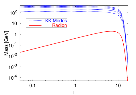
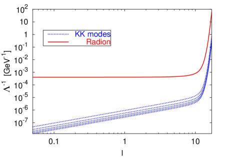
Figure 1: Mass (left panel) and coupling (right panel) of the radion and the first KK modes as a function of the (rescaled) amplitude $l$ of the scalar field. Parameters are chosen as $k=0.1\,M\,$, $u=k/40\,$, and in a way to maintain the same warping for all $l\,$.

Figure 1 shows the masses (left panel) and the couplings of the radion and the first (lightest) KK modes as a function of $l\,$. Besides $l\,$, the system is determined by the four parameter $M,\,k,\,u\,,$ and $y_{0}\,$ (or, equivalently, $w_{0}\,$). We fixed $u/k=1/40$ (too big or too small values give too small radion masses), and $k=0.1M\,$. The two additional conditions that we need are the recovery of the Plank mass in the $4$D gravity, eq. (34), and of the electroweak scale at the observable brane, eq. (36). The numerical results agree with the analytical expressions (37) at low $l\,$. The radion mass grows linearly with $l\,$, while the modes of the KK modes are constant. As $l$ increases, the masses show a rather sharp decrease, which extends also to greater values of $l\,$ than the ones shown in the Figure. The decrease is probably due to the increase of $w_{0}\,$, necessary to preserve a strong warping as $l$ increases (cf. eqs. (33) and (36)). We see that intermediate values for $l$ are needed, since the radion mass becomes too small both at small and large $l\,$. The maximum is achieved for $l~{}\mbox{\raisebox{-2.58334pt}{$\stackrel{{\scriptstyle<}}{{\sim}}$}}~{}10\,$, far from the $l\ll 1$ regime. Also the couplings of the modes to the observable sector, shown in the right panel, agree with the analytical results at small $l\,$. The coupling of the radion is constant, while the one of the KK modes increases linearly with $l\,$ (This behavior has been explained in the paragraph after eq. (37)). The coupling of all the modes sharply increases at large $l\,$, when the backreaction of $\phi$ cannot be neglected any longer. Both the decrease of the masses and the increase of the couplings occurring at large $l$ increase the potential detectability of the bulk excitations, and stringent experimental bounds should be expected in this limit.

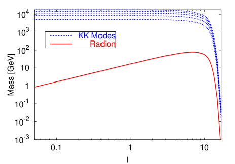
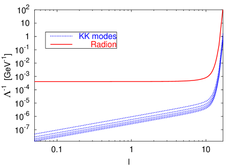
Figure 2: Same as in fig. 1, but with $k=M\,$.

An analogous calculation is summarized in Figure 2, where we show the masses and the couplings of the scalar modes for the choice of parameters $k=M\,$, $u=k/40\,$ ($y_{0}$ and $M$ are then fixed as in fig. 1). The numerical results shown in the two Figures exhibit the same qualitative behavior. The increase of $k$ is responsible for the higher values of the masses shown in fig. 2. The values of the couplings are instead very weakly sensitive on $k\,$, as eqs. (37) indicate.

IV.2 A Toy Braneworld

We consider a second example, characterized by the scalar potentials 

$$V\left(\phi\right) = -\,\tfrac{3\,W_{0}^{2}}{24\,M^{3}}\,{\rm exp}\left(\frac{2\,\phi}{\sqrt{3\,M^{3}}}\right)\,\,,$$

$$U_{\pm}\left(\phi\right) = \mp W_{0}\,{\rm exp}\left(\frac{\phi_{\pm}}{\sqrt{3\,M^{3}}}\right)\mp\frac{W_{0}}{\sqrt{3\,M^{3}}}\,{\rm exp}\left(\frac{\phi_{\pm}}{\sqrt{3\,M^{3}}}\right)\,\left(\phi-\phi_{\pm}\right)+\frac{\mu_{\pm}}{2}\,\left(\phi-\phi_{\pm}\right)^{2}$$ (38)

(see the previous subsection for the notation).

The background solutions for this model (given in conformal coordinate $y$ along the bulk) are

$$\phi=M^{3/2}\,\left[\alpha\,y+\beta\right]\;\;,\;\;A=\frac{2\,\sqrt{3}\,\alpha\,M^{3}}{W_{0}}\,{\rm e}^{-\,\frac{\alpha\,y+\beta}{\sqrt{3}}}\equiv A_{0}\,{\rm e}^{-\alpha\,y/\sqrt{3}}\,\,,$$ (39)

where $\alpha$ and $\beta$ are arbitrary constants (of mass dimension $1$ and $0\,$, respectively). Hence, the scalar field $\phi$ is linear in $y\,$. One can arrange for a strong warping between the two branes, $\alpha\,y_{0}\gg 1\,$. However, it is obtained through a strong hierarchy (in terms of the parameters entering in (38)) between the potentials $U_{\pm}$ at the two branes. In this sense, the model does not constitute a natural solution to the hierarchy problem. However, it is rather instructive, since the bulk equations for the perturbations of this model can be solved analytically (we have $z^{\prime\prime}/z=3\,\alpha^{2}/4$ in eq. (21)).

The junction conditions for the perturbations can be also solved analytically in the $\mu_{\pm}\rightarrow\infty$ limit . The mass spectrum is

$$m_{\rm rad}=\sqrt{\frac{2}{3}}\,\alpha\quad\quad,\quad\quad m_{\rm KK}=\sqrt{\frac{3\,\alpha^{2}}{4}+\left(\frac{n\,\pi}{y_{0}}\right)^{2}}\,\,.$$ (40)

The mass of the radion vanishes in absence of warping, while the KK modes have a contribution proportional to the warping in addition to the standard KK mass $\sim n\,\pi/y_{0}\;\left(n=1,\,2,\dots\right)\,$ . The masses of the radion and of the KK modes become comparable at large warping, $\alpha\,y_{0}\gg 1$. Finally, the coupling of the different modes to brane fields at the observable brane are given by

$$\Big{|}\frac{1}{\Lambda_{\rm radion}}\Big{|}=\frac{\alpha^{1/2}}{2^{1/2}\,3^{3/4}\,M^{3/2}\,A_{0}^{3/2}}\,{\rm e}^{\sqrt{3}\,\alpha\,y_{0}/2}\;\;,\;\;\Big{|}\frac{1}{\Lambda_{\rm KK}}\Big{|}=\frac{4\,n\,\pi\,\alpha^{1/2}}{3\,M^{3/2}\,A_{0}^{3/2}}\frac{1}{\left(\alpha\,y_{0}\right)^{3/2}}\,{\rm e}^{\sqrt{3}\,\alpha\,y_{0}/2}\,\,.$$ (41)

As in the previous example, the radion is more strongly coupled than the other KK modes, although the couplings have comparable strength.

V Numerics of the perturbations with the BraneCode

The analytical results derived above can be be supported by very different means, namely by the numerical study of the braneworld dynamics. Suppose we have a stable flat brane configuration plus fluctuations around it. This can be achieved by taking initial conditions which are slightly displaced from the stable configuration, so that the system will start oscillating around it. In this way we can study the properties and the time evolution of the perturbations, and see what relation they have with the eigemodes of the system computed analytically, eq. (27). The evolution of the interbrane distance $D\left(t\right)$ is often characterized by several oscillatory modes, superimposed to a lower frequency oscillation. Correspondingly, the Fourier transform of $D\left(t\right)\,$ shows the presence of resonance bands: the one with lowest frequency is identified with the radion field, while the other ones with the higher KK modes. The numerical values of the frequencies of the bands can be compared with the analytical expression for the masses of the modes. In addition, we can split the time evolution in successive time intervals (each containing several oscillations), and perform the Fourier transform in each of them. This allows to study how the excited modes evolve in time.

We make use of a numerical code, named BraneCode bc , designed for the study of the broad class of brane models (5) we are interested in. The numerical integration is performed with the assumption of homogeneity and isotropy along the brane coordinates, so that the system solved is effectively two-dimensional (time and bulk coordinates). This limitation removes the tensor modes from the numerical evolution (since there are no tensor modes in two dimensions), which is welcome for the present analysis. However, it also restricts the study of the scalar modes to the large wavelengths limit. Since we numerically integrate the exact $5$D Einstein equations, the present study goes beyond the linear regime for the perturbations, which limits instead the analytical calculations. In the example shown below, the nonlinear dynamics is relevant at the earlier stages of the evolution.

Some attention has to be paid to the choice of the initial conditions, since they have to respect two constraint (nondynamical) Einstein equations. The simplest possibility is to search for static bulk configurations, with

$$ds^{2}=A\left(y\right)^{2}\left[-dt^{2}+{\rm e}^{2Ht}\,d{\bf x}^{2}+dy^{2}\right]\,\,,$$ (42)

and with $\phi=\phi\left(y\right)\,$. As discussed in bc , the class of potentials considered in section IV admits at most two static configurations. When they exist, they are characterized by different values of $H\,$, which is proportional to the Hubble parameter measured by brane observers. The solution with higher $H$ is unstable, while the other one is stable. As explained in FK , a non-vanishing $H$ gives a negative contribution to the physical masses of the scalar fluctuations around the solution, $m_{\rm tot}^{2}\leq m_{0}^{2}-4\,H^{2}\,$. In many cases $m^{2}_{\rm tot}$ is negative, meaning that the corresponding static configuration is subject to a tachyonic instability FK . The instability typically leads towards the stable configuration, characterized by the lower expansion rate bc .

A systematic algorithm for the search of static configurations is described in bc . In the present discussion, we focus on the model (38), and start from an unstable static solution. Figure 3 shows the relaxation of this configuration towards a stable solution, of the class discussed in the previous section. We plot the time evolution of the interbrane distance, defined as

$$D\left(t\right)=\int_{0}^{y_{0}}dy\,A\left(t,y\right)\,\,,$$ (43)

together with its Fourier transform. We show two different spectra, according to different (consecutive) time intervals immediately after the “transition” between the two solutions.

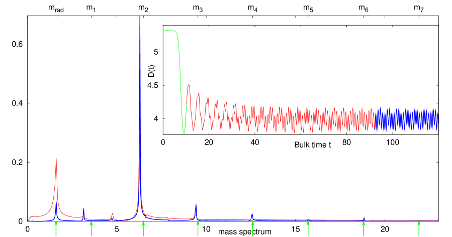
Figure 3: Relaxation towards a stable braneworld configuration in the model (38). The evolution of the interbrane distance $D\left(t\right)$ and its Fourier transform are shown. The arrows beneath the frequency axis denote the masses of the radion and of the first KK modes according to eq. (40). Parameters are chosen as $\alpha\,y_{0}=2,\,\beta=0,\,{\rm e}^{-\alpha\,y_{0}/\sqrt{3}}\,A_{0}\,\mu_{+}=A_{0}\,\mu_{-}=100\,M\,$, and the figure is shown in units $M=1\,$.

The numerical result confirms the rapidity of the transition, and the initial excitation of the radion mode. The subsequent evolution can be roughly divided into two stages. During the earlier one, we can see the excitation of modes of higher frequency superimposed to the radion oscillation. The positions of the modes are in excellent agreement with the masses obtained analytically - see eq. (40) - which are indicated by the arrows below the frequency axis. These confirm that the modes excited are precisely the ones found through the linearized analytical calculation. We note that the excitation of the higher modes starts already during the first oscillation of the radion field. It is also possible to see a decrease of the amplitude of the radion oscillations during all this first stage. The second stage is instead characterized by a constant pattern of oscillatory modes. The spectrum of the perturbations does not change appreciably during these later times.

These features can be readily understood. The large amplitude of the radion oscillations is due to the strong tachyonic instability of the first configuration. The excitation of the higher frequency modes is due to the coupling of the perturbations which occurs at the nonlinear level (as we mentioned, the numerical integration automatically takes into account the nonlinear dynamics of the system). Most of the energy of the radion field is transferred to the higher modes, as also indicated by the decrease of the overall amplitude occurring in the first stage. At later times, the amplitudes of the oscillations become sufficiently small so that nonlinear effect can be neglected. The fact that the patterns of the oscillations become constant confirms that the modes are decoupled at the linear level, as eq. (27) indicates.

In the present computation, we did not include any brane fields. Their coupling to the radion may be responsible for some energy transfer from the bulk to fields on the brane, during the earlier stages of cosmological evolution. This possibility is discussed in greater detail in the discussion section.

VI Discussion

We considered $5$D braneworld models with the inclusion of a bulk scalar field for the sake of generality and, more importantly, to provide stabilization of the extra dimension. Observers on a $4$D brane embedded in this space will in general experience corrections to the $4$D Einstein gravity, as well as additional four dimensional degrees of freedom emerging from the bulk gravity and the bulk scalar. These excitations interact with the fields of the Standard Model (or more generically, of the observable sector) living on our brane. Therefore, their nature and the details of their couplings to the observable sector are the subject of particle physics phenomenology and experiments. The set-up we studied is a specific example of more general systems characterized by a higher dimensional warped bulk geometry, which emerges not only in the context of $5$D braneworlds, but also in many other models motivated by string cosmology, see e.g. KKLT . For this reason we will comment not only on the results of the explicit calculations of the paper, but also on potential extensions of our methods and results for the broad context of the warped geometries.

In the present paper we focused on the scalar excitations of the system. The warp bulk geometry can be strongly curved, and the full machinery of General Relativity is required for the study of the bulk gravity/scalar dynamics. In general, the physical modes associated with the excitations of the coupled gravity/scalar system do neither coincide with the fluctuations $\delta\phi$ of the scalar field nor with the scalar perturbations $\Phi$ of the metric, but rather with some linear combination of them. This is sharply different from the identification of the eigenmodes in the familiar KK dimensional reduction, where higher dimensional metric components decouple from the bulk fields. A much more similar context is the one of $4$D cosmology with scalar fields, where cosmological scalar perturbations of the metric are sourced by the fluctuations of the inflaton. In the present paper we extended this approach to the more complicated set-up of higher dimensional warped geometries.

This analysis can be pursued in several directions.

1. We computed the coupling of the radion (the lightest eigenmode of the warped geometry excitations) and of the higher KK modes to Standard Model particles, which is one of the most crucial pieces of information for phenomenological studies. The physical modes emerge from the decomposition and diagonalization of the second order action for the perturbations. The diagonalization requires great care, since the starting action for the perturbations is particularly involved, and the identification of the relevant dynamical variables is far from being obvious. Contributions both from the bulk and the branes are present in this action, neither of which can be immediately diagonalized. In particular, a priori one could have wondered whether the two different contributions could have been simultaneously diagonalized, or if some mixing between the different KK levels would have unavoidably remained.

We performed this tedious decomposition in the case of $5$D braneworlds with bulk scalar field and two orbifold branes at the edges. The answer happens to be rather transparent and simple: the total action for the perturbations from the bulk and the two branes can be diagonalized in terms of free, non-interacting scalar KK excitations. The canonical quantization of the actions of these modes specifies the normalization of their wave function along the extra dimension. This in turns defines the value of the perturbations at the observable brane, which sets the coupling between the scalar modes and the SM fields (the overall normalization cannot be obtained from the $5$D Einstein equations for the perturbations, which are all linear in the perturbations). For the reasons just remarked, it should not be a surprise that the couplings are very sensitive on the details of background bulk geometry and of the bulk scalar field distribution. We illustrated this dependence with some specific examples, see for example Figs. 1 and 2.

One of the examples we have considered is related to the Goldberger-Wise mechanism GW for the stabilization of the Randall-Sundrum model RS1 . More specifically, we consider the model by De Wolfe et al. (DFGK) Dewolfe , where the background equation for the stabilized geometry and the bulk scalar field can be solved analytically. It is convenient to introduce a parameter $l$ csaki2 - proportional to the amplitude of the scalar field - which characterizes the departure of the model from the pure Randall-Sundrum model without stabilization. Thus, $l=0$ corresponds to the Randall-Sundrum model, small $l\ll 1$ to small backreaction of the background scalar on the bulk AdS geometry, while large $l~{}\mbox{\raisebox{-2.58334pt}{$\stackrel{{\scriptstyle>}}{{\sim}}$}}~{}1$ implies a significant modification of the geometry due to the presence of $\phi\,$. It is important to bear in mind that a large warping (large difference of the background conformal factor $A$ between the two branes) can be obtained for all $l\,$. Thus, the virtue of the braneworld models to solve the hierarchy problem is preserved also for cases, characterized by large $l\,$, in which the bulk geometry may significantly differ from the AdS geometry of RS1 . Indeed, in the specific example we have considered we were able to preserve the same warping for all values of $l\,$.

We shall make comment on the physical reliability of the models with small vs. non-small $l$. It is not easy to accept that the bulk scalar field gives only negligible, perturbative contribution to the background bulk geometry, and that its only role is to provide a tiny lift of the radion mode, without affecting the geometry in any other way. As we already remarked, the idea of RS is to avoid strong hierarchies besides the one given by the warp factor. If $l$ is limited to the small values needed to remain in the perturbative regime, the radion mass turns out to be significantly smaller than the electroweak scale. Although this is certainly a much milder hierarchy than the one between the electroweak and the Plank scales, it can be avoided provided $l$ is sufficiently large. Another point in favor of a large $l$ is related to the dynamics of the radion in the early universe. To appreciate this, we computed and showed in Appendix C the $4$D effective potential for the radion (this effective potential is only approximately valid at small $l\,$, and should not be confused with the exact $4$D description given in the main text). In terms of the canonically normalized field (corresponding to the radion in this effective description), the local minimum at which the stabilization occurs is minuscule. If we are interested in the early dynamics of the braneworld, it is very hard to understand how the system can go to such a minimum, unless it starts extremely close to it. This is a very similar problem to the one of moduli stabilization in heterotic string cosmology bs . This problem is enhanced for small $l\,$. These reasons are a strong motivation for studying the system also beyond the small $l$ limit.

The coupling of the radion to SM fields was already computed by Csaki et al. csaki2 in the limit of small backreaction, $l\ll 1\,$. Our formula reproduces their result in this limit. In addition, we found that the strength of the interaction remains almost constant in the range $0<l~{}\mbox{\raisebox{-2.58334pt}{$\stackrel{{\scriptstyle<}}{{\sim}}$}}~{}10$. Most interestingly, however, is that for $l>10$ the value of the coupling begins to grow sharply as a function of $l$. Therefore we conclude that, in the model considered, a stronger stabilization can enhance even by orders of magnitude the coupling of the radion to SM fields.

Another very interesting property we found is the strong dependence of the masses of the radion and of the KK modes on the parameter $l\,$. In the range $0<l~{}\mbox{\raisebox{-2.58334pt}{$\stackrel{{\scriptstyle<}}{{\sim}}$}}~{}10$ the mass of the radion increases linearly with $l$ (consistently with the fact that the radion becomes massless as $l\rightarrow 0\,$), while the masses of the KK modes are nearly constant. At $l~{}\mbox{\raisebox{-2.58334pt}{$\stackrel{{\scriptstyle>}}{{\sim}}$}}~{}10$ the masses of all the modes are instead sharply decreasing. The decrease is probably due to the larger interbrane separation which must be imposed at large $l\,$ - in order to preserve a strong warping at the observable brane - and which results in lower masses from gradients in the $y$ direction. Hence, both very small and large $l$ are phenomenologically excluded, since they lead to a too light radion. The radion mass is maximized for $l\sim 10\,$, far from the perturbative $l\ll 1$ regime. This paper provides the technical tools for extending the phenomenological studies to this relevant regime.

2. We identified the KK eigenmodes of the braneworld excitations in the general case, without any assumption of small backreaction of the bulk scalar field. In the linear regime they are free non-interacting dynamical fields, since they correspond to canonically normalized eigenmodes of the action expanded up to second order in the perturbations. However, we may expect that they are coupled at higher (third and further) order in the decomposition of the full action. To verify this, we made use of numerical simulations of the dynamical evolution of the braneworlds, which give complementary informations to the analytical study. The simulations are based on the BraneCode, which was developed to solve the fully nonlinear self-consistent evolution of the braneworld with the scalar field bc . We started with an unstable brane configuration, which evolves to a stable one plus excitations around it. The excitations are composed of a superposition of oscillatory modes, whose frequencies (determined by a Fourier decomposition) coincide with the eigenmasses found by the analytical study of the linear regime. The higher KK modes are excited by the nonlinear interactions with the radion field during the earlier stages of the evolution. At later times, the nonlinear interactions can be neglected, and the pattern of oscillations becomes constant.

The discussion of the brane system restructuring and of the excitation of its eigenmodes leads us to another subject where the interaction of the radion and the other KK modes with SM particles is important. This is (p)reheating of the universe after inflation, and, in particular, the role that the brane excitations may have had in the generation of brane fields. Inflation in the braneworld setting corresponds to the curved brane, so that after inflation the brane is flattening as the brane curvature decreases with the decrease of the Hubble parameter $H(t)$. As we just noted, the reconfiguration of the brane geometry leads to interbrane oscillations, which correspond to excitations of the radion and the other KK modes. The interaction of the bulk modes with the SM particles will results in the decay of these oscillations. More specifically, let us consider a coherently oscillating radion $\Phi=\Phi_{0}\,\cos{m_{rad}\,t}$ interacting with some scalar field $\chi$ of mass $m$ living on our brane. The equation for the amplitudes of the eigenmodes $\chi_{k}(t)e^{i\vec{k}\vec{x}}$ of quantum fluctuations of $\chi$ can be reduced to

$$\ddot{\chi}_{k}+\left(k^{2}+m^{2}-(m^{2}+\frac{1}{2}m^{2}_{rad})\Phi_{0}\,\cos{m_{rad}\,t}\right)\chi_{k}=0$$ (44)

(more accurately, $\chi_{k}$ refers to the canonically normalized field, and $m$ to the physical mass, both obtained after a rescaling with the conformal factor at the brane; in addition, one should take into account that the amplitude $\Phi_{0}$ of the oscillations is decreasing due to the cosmological expansion of the brane). This is the familiar equation for the parametric resonant amplification of quantum fluctuations interacting with the oscillating background field KLS94 . The strength of the effect is given by the parameter $q=(\frac{m^{2}}{m^{2}_{rad}}+\frac{1}{2})\,\Phi_{0}$. The amplitude of the radion oscillations (here $\Phi_{0}$) corresponds to the induced metric fluctuation, which is below unity. Thus, in case of a mass ratio $\frac{m^{2}}{m^{2}_{rad}}<1\,$, the parametric resonance is not strong enough for preheating. In the opposite case, $\frac{m^{2}}{m^{2}_{rad}}\gg 1\,$, the parameter $q$ is large, but the effect works only in the higher instability bands where $k^{2}>\frac{m^{2}}{m^{2}_{rad}}\,$, and it is again very small. We conclude that it is hard to have preheating effects from the radion oscillations, so that the radion oscillations decay in the perturbative regime. An interesting earlier paper coll seems to conclude that preheating effects associated to the oscillations of the radion are instead more significant. We think that, once the expansion of the brane, and the consequent decrease of the amplitude of the oscillations, are taken into account, the result claimed in coll may be significantly reduced.

3. Finally, we will discuss other virtues of the method of the full action series decomposition which we used in the paper. While we focus on the problem of identification of the eigenmodes of the gravity/scalar dynamical system in order to quantize the radion and the higher KK modes, in principle we can extend this method to discuss another important sector of the effective $4$D theory, namely effective $4$D gravity. There is extensive literature on the properties of the $4$D gravity in the braneworld models; here we discuss only the low energy limit, that is the linearized gravity at the brane cgr ; shift ; Mukohyama:2001ks . On general grounds, one expects that the $4$D effective gravity at the brane will be a Brans-Dicke (BD) theory. For pure RS model without brane stabilizations, the BD gravity contains a massless scalar, which is the radion. For stabilized branes the radion acquires a mass, so that one expects a BD theory with a massive BD scalar. The latter situation was studied in R , where the Lagrangian for the $4$D gravity was derived as a series containing the Einstein term $R$ plus higher derivatives term of the form $R^{2}/m^{2}_{rad}$, plus even higher derivatives terms.

The main method adopted in the literature for the derivation of the low energy $4$D effective gravity is based on the introduction of a point-like stress-energy source at the visible brane, and on the investigation of the gravitational response upon this source, including the bulk gravity, the scalar field, and the shift in the embedding of the branes shift . Notice, however, that the signature of the low energy gravity (BD or $R^{2}$ theory) is manifested in the free gravitational modes even without the stress-energy sources. Therefore, in principle we can address the question regarding brane gravity in terms of the series decomposition of the full action. To do so, we need to include not only the scalar metric perturbations $\Phi$ in the form (6), but also the transverse-traceless gravitational modes $h^{TT}_{AB}$. Bulk gravitational waves in general have $5$ degrees of freedom. However, the massless scalar and vector projections of the bulk graviton are absent, so that the massless graviton has only $2$ degrees which corresponds to usual $3+1$ dimensional transversal and traceless (TT) gravitational waves $h^{TT}_{\mu\nu}\,$ andrei . We can extend (6) to the form where the full $5$D metric perturbations $h_{AM}$ are

$$h_{55}=2\Phi\ ,\,\,\,h_{5\mu}=0\ ,\,\,\,h_{\mu\nu}=h^{TT}_{\mu\nu}-\eta_{\mu\nu}\Phi\ .$$ (45)

We then have to include TT modes in the decomposition of section III.1. Up to the second order in perturbation series, the effective $4$D action acquires the new term $h^{TT}_{\mu\nu;\rho}h^{TT;\rho}_{\mu\nu}/4$ which is equal to the linearized $4$D curvature $R$, see e.g. andrei . The BD coupling $(1+Q)R$ emerges only in the third order of the perturbation series, which is beyond the scope of this paper. Here we just note that a terms with the structure $\Phi h^{TT;\rho}_{\mu\nu}h^{TT}_{\mu\nu;\rho}$ will appear in the third order decomposition.

What is important, is that with the present approach we explicitly see that the BD scalar is a massive one. This follows from the second order decomposition of section III.2. Now, how the BD theory with the massive radion (as a BD scalar) can be reconciled with the $R+R^{2}$ theory derived in R ? It is well known conf that a theory of gravity with the higher derivatives in the form ${\cal L}_{1}=-\frac{M_{p}^{2}}{16\pi}\left(R+\frac{R^{2}}{6m^{2}}\right)$ is conformally equivalent to the Einstein theory with the scalar field $\phi$ and with Lagrangian ${\cal L}_{2}=-\frac{M_{p}^{2}}{16\pi}R+\frac{1}{2}\phi_{\mu}\phi^{\mu}-V(\phi)$. The metrics of theories ${\cal L}_{1}$ and ${\cal L}_{2}$ are related by conformal transformation $g_{\mu\nu}\to\left(1-\frac{R}{3m^{2}}\right)\,g_{\mu\nu}$. The scalar fields $\phi$ is obtained from the scalar curvature $R$ as

$$\phi=\sqrt{\frac{3M_{p}^{2}}{16\pi}}\ln\left(1-\frac{R}{3m^{2}}\right)\,\,,$$ (46)

and the potential is given by formula

$$V(\phi)=\frac{3M_{p}^{2}m^{2}}{32\pi}\left[1-\exp\left(-\sqrt{\frac{16\phi}{3M_{p}^{2}}}\phi\right)\right]\ .$$ (47)

In the limit of small $\phi$ we obtain $V(\phi)\approx\frac{1}{2}m^{2}\phi^{2}$. Thus, for small values of the radion (i.e. BD scalar) the Einstein gravity with small high derivative corrections is equivalent to the theory without $R^{2}$ term but with instead the additional massive scalar.

Appendix A Computation of $S_{2}$

In this Appendix we outline the computation of the action (18) for the perturbations. Following mfb , we first perform an ADM decomposition along $y$ of the gravitational part of the action (5). One can easily verify that, for a line element of the form

$$ds^{2}={\cal A}^{2}\left(t,{\bf x},y\right)\left(-dt^{2}+d{\bf x}^{2}\right)+{\cal B}^{2}\left(t,{\bf x},y\right)dy^{2}\,\,,$$ (48)

one has

$$\sqrt{|G|}R=\sqrt{|G|}\left\{R_{\left(4\right)}+\frac{12\,{\cal A}^{\prime 2}}{{\cal B}^{2}\,{\cal A}^{2}}\right\}-8\left[\frac{{\cal A}^{3}\,{\cal A}^{\prime}}{{\cal B}}\right]^{\prime}-2\,\eta^{\mu\nu}\partial_{\mu}\left({\cal A}^{2}\,\partial_{\nu}{\cal B}\right)\,\,,$$ (49)

where $R_{\left(4\right)}=-6\eta^{\mu\nu}\left(\partial_{\mu}\partial_{\nu}{\cal A}\right)/{\cal A}^{3}$ is the curvature of the four dimensional slices. The last term in (49) is a boundary term on the $3+1$ slices, and it can be dropped. On the other hand, the total derivative in $y\,$ does not vanish, since the space in that direction is limited by the two branes. However, its contribution to the action precisely cancels with the Gibbons-Hawking term $\sqrt{-\gamma}\left[K\right]$ in the starting action (5) for the two branes.

Hence, only the first term of (49) is relevant. Combining it with the bulk action for the scalar field, we get

$$S_{\rm bulk}=2\int_{0}^{y_{0}}d^{5}x{\cal A}^{4}\,{\cal B}\left[-6\,M^{3}\,\eta^{\mu\nu}\frac{\partial_{\mu}\partial_{\nu}{\cal A}}{{\cal A}^{3}}+\frac{12\,M^{3}\,{\cal A}^{\prime 2}}{{\cal B}^{2}\,{\cal A}^{2}}-\frac{\eta^{\mu\nu}}{2\,{\cal A}^{2}}\partial_{\mu}\varphi\,\partial_{\nu}\varphi-\frac{1}{2\,{\cal B}^{2}}\varphi^{\prime 2}-V\right]\,\,.$$ (50)

The coefficients ${\cal A}$ and ${\cal B}$ are obtained from the line element (6). Expanding the bulk action at second order in the perturbations, and making use of the background equations to simplify the final expression, we obtain the bulk part of the action (18). The brane contributions to (18) are instead the expansion of the last term of (5).

Appendix B Perturbations in the DFGK model for $l\ll 1$

In the following, we derive the analytical results given in (37), valid in the $l\ll 1$ regime. Some of the present results were also obtained in csaki2 . It is useful to work in terms of the rescaled mode ${\tilde{Y}}_{n}=A^{2}\,{\tilde{\Phi}}_{n}\,$, and in normal coordinate $w\,$. By combining the equations for the background quantities and the perturbations, one finds

$${\tilde{Y}}_{n}^{\prime\prime}-2\left(\frac{\phi^{\prime\prime}}{\phi^{\prime}}+\frac{A^{\prime}}{A}\right){\tilde{Y}}_{n}^{\prime}+\left[2\,\frac{A^{\prime\prime}}{A}-2\,\frac{A^{\prime 2}}{A^{2}}+\frac{m_{n}^{2}}{A^{2}}\right]{\tilde{Y}}_{n}=0\quad\quad,\quad\quad{\tilde{Y}}_{n}^{\prime}|_{w=0,w_{0}}=0$$ (51)

(in this Appendix, prime denotes differentiation with respect to normal coordinate $w\,$).

For the moment, we restrict the computation to $l=0\,$, that is we ignore the backreaction of the scalar field on the background geometry (notice that $\phi^{\prime\prime}/\phi^{\prime}=-u$ is regular in this limit). The bulk equation is then solved by

$${\tilde{Y}}_{n}={\tilde{Y}}_{n}^{(0)}\,{\rm e}^{-w\left(k+u\right)}\left[J_{1+u/k}\left(\frac{m_{n}}{k}\,{\rm e}^{kw}\right)+{\cal C}_{n}\,Y_{1+u/k}\left(\frac{m_{n}}{k}\,{\rm e}^{kw}\right)\right]\,\,,$$ (52)

with arbitrary constants ${\tilde{Y}}_{n}^{(0)}$ and ${\cal C}_{n}\,$. Differentiating this solution gives

$${\tilde{Y}}_{n}^{\prime}=-m_{n}\,{\tilde{Y}}_{n}^{(0)}\,{\rm e}^{-w\,u}\left[J_{2+u/k}\left(\frac{m_{n}}{k}\,{\rm e}^{kw}\right)+{\cal C}_{n}\,Y_{2+u/k}\left(\frac{m_{n}}{k}\,{\rm e}^{kw}\right)\right]\,\,.$$ (53)

The boundary condition at $w=0$ can be used to enforce

$${\cal C}_{n}=-\,\frac{J_{2+u/k}\left(\frac{m_{n}}{k}\right)}{Y_{2+u/k}\left(\frac{m_{n}}{k}\right)}\rightarrow\frac{\pi}{\Gamma\left(2+\frac{u}{k}\right)\,\Gamma\left(3+\frac{u}{k}\right)}\,\left(\frac{m_{n}}{2\,k}\right)^{4+\frac{2\,u}{k}}\,\,,$$ (54)

where the last limit holds for $m_{n}/k\rightarrow 0\,$. As we will now see, this is the case we are interested in, since $m$ is set to the electroweak scale, while $k\sim M_{p}\,$.

Eq. (53) shows that a mode (52) with vanishing mass solves also the boundary conditions. This mode corresponds to the radion, whose mass is due to the backreaction of $\phi$ on the geometry: a non-vanishing radion mass is found only once the bulk equation (51) is expanded at the first nontrivial order in $l\,$. Let us postpone this calculation till the end of this Appendix, and concentrate on the KK modes, for which the present calculation ($l=0$) is accurate enough. As clear from the expansion (54), the second term in (52) is completely irrelevant for $m_{n}/k\sim{\rm TeV}/M_{p}\,$. The junction condition at $w=w_{0}$ then gives

$$J_{2+\frac{u}{k}}\left(\frac{m_{n}}{k}\,{\rm e^{k\,w_{0}}}\right)\simeq 0\,\,.$$ (55)

Hence, the masses of the KK modes are determined by the poles of this function. By expanding it for large argument we find

$$m_{n}\simeq\frac{\pi}{y_{0}}\left[n+\frac{3}{4}+\frac{u}{2\,k}-\frac{15+16u/k+4u^{2}/k^{2}}{8\,\pi^{2}\,n}+{\cal O}\left(n^{-2}\right)\right]\quad,\quad\quad n=1,\,2,\,3,\,4,\,5,\dots$$ (56)

This approximation becomes more and more accurate as $n$ increases. However, the comparison with numerical results shows very good agreement at all $n\,$. The normalization coefficient ${\tilde{Y}}_{n}^{(0)}$ is computed by inserting the solution (52) into the normalization condition (27). Since we are interested in the leading result for small $l\,$, only the first term in (27) has to be computed. We get

$$\frac{9\,M^{3}\,m_{n}^{2}\,{\tilde{Y}}_{n}^{(0)\>2}}{8\,l^{2}\,u^{2}}\,\int_{0}^{w_{0}}dw\,{\rm e}^{2\,k\,w}\,J_{2+\frac{u}{k}}^{2}\left(\frac{m_{n}}{k}\,{\rm e}^{k\,w}\right)\simeq\frac{9\,M^{3}\,{\tilde{Y}}_{n}^{(0)\>2}}{16\,k\,l^{2}\,u^{2}}\,m_{n}^{2}\,{\rm e}^{2\,k\,w_{0}}\,J_{1+\frac{u}{k}}^{2}\left(\frac{m_{n}}{k}\,{\rm e}^{k\,w_{0}}\right)\equiv\frac{1}{2}\,\,.$$ (57)

We can now evaluate the normalized ${\tilde{\Phi}}_{n}={\tilde{Y}}_{n}/A^{2}$ at the $w_{0}\,$ brane. We obtain, at leading order, the coupling of the KK modes with brane fields reported in eq. (37).

We still have to compute the normalization and the mass of the radion field. As remarked, the mass can be obtained by inserting the background solutions (33) into the bulk eq. (51), and expanding at the first nontrivial order in $l\,$. The normalization can however be found already from the $l=0\,$ term. At zero-th order in $l\,$, the radion is massless, and eqs. (51) are solved by a constant ${\tilde{Y}}\,$ (as it is also confirmed by the limit of (53) and (54) for $m_{n}\rightarrow 0\,$). We thus recover the result ${\tilde{\Phi}}\propto A^{-2}$ given in (14). Inserting a constant ${\tilde{Y}}$ in (27) we find the radion normalization, and finally the coupling to SM fields given in eq. (37). The radion mass is obtained by expansion of the bulk eq. (51) at second order in $l\,$, using the ansatz ($Y_{0}$ is the constant $0-$th order solution)

$$Y\left(w\right)=Y_{0}+l^{2}y\left(w\right)\;\;,\;\;\;m^{2}=l^{2}{\tilde{m}}^{2}\,\,.$$ (58)

This equation can be easily solved. Imposing that $y^{\prime}\left(w\right)$ vanishes at the two branes gives the radion mass

$$m^{2}=\frac{4\,l^{2}\,u^{2}\,\left(2k+u\right)\left({\rm e}^{2\,k\,w_{0}}-1\right)}{3\,k\left({\rm e}^{2\left(2k+u\right)w_{0}}-1\right)}\simeq\frac{4\,l^{2}\,u^{2}\left(2k+u\right){\rm e}^{-2\left(k+u\right)w_{0}}}{3\,k}\,\,.$$ (59)

The function $y\left(w\right)$ modifies the radion normalization at subleading order in $l\,$; the effect can be neglected provided $l$ is sufficiently small.

Appendix C Effective potential for the radion

In this Appendix we compute the effective $4$D Lagrangian for the radion in the model (IV.1), following the original computation of GW . The $4$D Lagrangian is obtained starting from an ansatz which does not satisfy the $5$D Einstein equations of the theory, so it should be considered only as a first, heuristic study of the system. We discuss it here mainly to compare it with the exact $4$D description obtained in section III. To derive it, it is convenient to use “rescaled” normal coordinates

$$ds^{2}=A\left({\bar{w}}\right)^{2}\eta_{\mu\nu}\,dx^{\mu}\,dx^{\nu}+w_{0}\left(t\right)^{2}d{\bar{w}}^{2}\quad,\quad\quad{\bar{w}}\in\left[0,1\right]\,\,,$$ (60)

so that the interbrane distance is encoded in the (time-dependent) parameter $w_{0}\,$. The advantage of this parameterization is that the kinetic term for $w_{0}\,$ is very easily obtained. As in GW , we neglect the backreaction of the scalar field $\phi$ on the metric; hence, the analysis is restricted to the small $l$ limit (in addition, the effective Lagrangian only refers to the radion field, while the result (27) is valid for all the physical modes). We “promote” the parameter $w_{0}$ to be time-dependent, so that

$$A={\rm e}^{-k\,{\bar{w}}\,w_{0}\left(t\right)}\,\,.$$ (61)

The kinetic term for $w_{0}$ is obtained by integration over ${\bar{w}}$ of the $R_{\left(4\right)}$ term in (49), which gives

$${\cal L}_{K}=M^{3}\int_{0}^{1}d{\bar{w}}\,w_{0}A^{4}\frac{6\,\ddot{A}}{A^{3}}=\dots=\frac{1}{2}\left[\sqrt{\frac{6\,M^{3}}{k}}\,{\rm e}^{-kw_{0}\left(t\right)}\right]^{{\small\bullet}\,2}\equiv\frac{1}{2}\dot{\gamma}^{2}\left(t\right)\,\,,$$ (62)

where $\gamma$ is the canonically normalized field (a further contribution to ${\cal L}_{K}$ is given by the kinetic term of $\phi\,$, but it is subdominant in $l\,$).

The effective potential for the radion is obtained by integrating the action over ${\bar{w}}\,$. The O$\left(l^{0}\right)$ part cancels, corresponding to the cancellation of the $4$D cosmological constant in the RS model. Hence, we effectively integrate the action for the scalar field, after subtracting the bulk cosmological constant and the brane tensions from the bulk/brane potentials

$$-V_{\rm eff}=2\int_{0}^{1}d{\bar{w}}\,A^{4}w_{0}\left[-\frac{\phi^{\prime 2}}{2\,w_{0}^{2}}-{\tilde{V}}\right]-A\left(0\right)^{4}{\tilde{U}}_{0}-A\left(1\right)^{4}{\tilde{U}}_{1}$$ (63)

(in this Appendix, prime denotes differentiation with respect to ${\bar{w}}\,$). The rescaled potentials are (cf. eqs. (IV.1))

$${\tilde{V}} = \left(2\,k\,u+\,\frac{u^{2}}{2}\right)\phi^{2}+{\rm O}\left(\phi^{4}\right)\,\,,$$

$${\tilde{U}}_{0} = -2\,u\,l^{2}M^{3}-2\,\sqrt{2}\,l\,u\,M^{3/2}\left(\phi\left(0\right)-\sqrt{2}\,l\,M^{3/2}\right)+\frac{\mu_{+}}{2}\left(\phi\left(0\right)-\sqrt{2}\,l\,M^{3/2}\right)^{2}\,\,,$$

$${\tilde{U}}_{1} = 2\,u\,l^{2}M^{3}\,{\rm e}^{-2\,u\,q_{0}}+2\,\sqrt{2}\,l\,u\,M^{3/2}\,{\rm e}^{-u\,q_{0}}\,\left(\phi\left(1\right)-\sqrt{2}\,l\,M^{3/2}\,{\rm e}^{-u\,q_{0}}\right)+\frac{\mu_{-}}{2}\left(\phi\left(1\right)-\sqrt{2}\,l\,M^{3/2}\,{\rm e}^{-u\,q_{0}}\right)^{2}\,.$$ (64)

Contrary to this Appendix, in the other parts of this paper the background solution is fixed to the static configuration determined by the bulk/brane potentials. In the present calculation, this would amount in setting $w_{0}=q_{0}\,$ (this can be easily seen by comparing the value of $A$ at the second brane with the potential on that brane, as given here and in section IV.1). However, our aim here is to compute the effective potential for arbitrary $w_{0}\,$, so that the bulk ansatz for $A\left({\bar{w}}\right)$ and for $\phi\left({\bar{w}}\right)$ has to be given also for $w_{0}\neq q_{0}\,$. As we shall see, the effective potential $V_{\rm eff}$ will be precisely minimized for $w_{0}=q_{0}\,$, in agreement with the exact equations of the $5$D theory.

The bulk equation for $\phi$ in the unperturbed background (61) is

$$\phi^{\prime\prime}-4\,k\,w_{0}\,\phi^{\prime}-w_{0}^{2}\left(4\,k\,u+u^{2}\right)\phi=0\,\,.$$ (65)

In addition, we have the boundary conditions at the two branes, which, in the large $\mu_{\pm}$ limit, read

$$\phi\left(0\right)=\sqrt{2}\,l\,M^{3/2}\quad\quad,\quad\quad\phi\left(1\right)=\sqrt{2}\,l\,M^{3/2}\,{\rm e}^{-u\,q_{0}}\,\,.$$ (66)

These equations give

$$\frac{\phi\left({\bar{w}}\right)}{\sqrt{2}\,l\,M^{3/2}}=\left[1-\frac{{\rm e}^{\left(w_{0}-q_{0}\right)u}-1}{{\rm e}^{2\left(2k+u\right)w_{0}}-1}\right]\,{\rm e}^{-uw_{0}{\bar{w}}}+\frac{{\rm e}^{\left(w_{0}-q_{0}\right)u}-1}{{\rm e}^{2\left(2k+u\right)w_{0}}-1}\,{\rm e}^{\left(4k+u\right)w_{0}{\bar{w}}}\,\,.$$ (67)

We note that, for $w_{0}=q_{0}\,$, the expression (67) reduces to $\phi=\sqrt{2}\,l\,M^{3/2}\,{\rm exp}\left(-uq_{0}{\bar{w}}\right)\,$, in agreement with eq. (33). The effective potential for the radion is now easily computed to be

$$V_{\rm eff}=\frac{4\,l^{2}\,M^{3}\left(2k+u\right)\left[{\rm e}^{u\left(w_{0}-q_{0}\right)}-1\right]^{2}}{{\rm e}^{2\left(2k+u\right)w_{0}}-1}+{\rm O}\left(l^{4}\right)\,\,.$$ (68)

which is indeed minimized (and vanishes) for $w_{0}=q_{0}\,$.

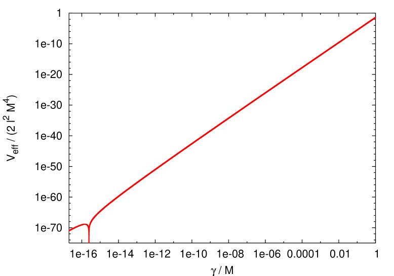
Figure 4: Effective $4$D potential as a function of the canonically normalized field $\gamma\,$. We fixed $k=M,\,u=M/40\,$. The parameter $q_{0}$ is chosen so that ${\rm exp}\left(-k\,q_{0}\right)=10^{-16}$ sets the electroweak scale at the observable brane. Note that the interbrane distance decreases as $\gamma$ increases.

To summarize the computation, the effective $4$D Lagrangian for the radion is, in terms of the canonically normalized field $\gamma\,$ and at leading order in $l\,$,

$${\cal L}_{\rm eff}=\frac{1}{2}\,\dot{\gamma}^{2}-V_{\rm eff}\quad\quad,\quad\quad V_{\rm eff}=4\,l^{2}\,M^{3}\left(2k+u\right)\frac{\left[{\rm e}^{-u\,q_{0}}\left(\sqrt{\frac{k}{6\,M^{3}}}\,\gamma\right)^{-u/k}-1\right]^{2}}{\left(\sqrt{\frac{k}{6\,M^{3}}}\,\gamma\right)^{-2\left(2k+u\right)/k}-1}\,\,.$$ (69)

In Figure 4 we show $V_{\rm eff}\left(\gamma\right)$ for a specific choice of the parameters compatible with the solution of the hierarchy problem (see the main text). We note that the interbrane distance decreases as $\gamma$ increases. The limit $\gamma\rightarrow 0$ ($w_{0}\rightarrow\infty$) corresponds to infinite distance between the two branes, while the two branes coincide for $\gamma=\sqrt{6\,M^{3}/k}$ ($w_{0}=0\,$). The potential $V_{\rm eff}$ sharply increases as the two branes approach each other, due to the strong gradient energy of $\phi\,$. On the contrary, $V_{\rm eff}$ vanishes at very large distances (small $\gamma\,$). In addition, $V_{\rm eff}$ has a minimum at finite $\gamma\equiv\gamma_{0}\,$, corresponding to $w_{0}=q_{0}\,$. This is the value of the radion set by the stabilization mechanism.

We should caution against the use of this potential for a strongly time-dependent $\gamma\left(t\right)\,$, and for $\gamma$ too far from the minimum $\gamma_{0}\,$. Indeed, the starting ansatz (61) and (67) does not satisfy the Einstein equations of the $5$D theory even in the small $l$ limit. More accurate answers can be obtained from the (numerical) integration of the equations of the exact $5$D theory bc . Still, the effective potential can be used to gain a qualitative understanding of the system. We see that $\gamma$ has to be always very close to $\gamma_{0}\,$, if we want the stabilization to take place. We note the close analogy with to the problem of stabilizing the dilaton of superstring theory from gaugino condensation bs : starting from a static configuration far from $\gamma_{0}\,$, the two branes will move to infinite distance, since the barrier in the potential at $\gamma~{}\mbox{\raisebox{-2.58334pt}{$\stackrel{{\scriptstyle<}}{{\sim}}$}}~{}\gamma_{0}$ is too small to “stop” the evolution of the two branes, unless $\gamma\simeq\gamma_{0}$ from the very beginning. Although this problem is present at all $l\,$, the scale of the potential shows that it becomes worse as $l$ decreases, since one can start from smaller interbrane distance without $V_{\rm eff}$ to exceed the limit of validity of the computation (e.g. $V_{\rm eff}$ smaller than the scale set by the AdS curvature).

The effective potential (69) allows a very accurate determination of the mass of the radion in the small $l$ limit

$$m_{\rm eff}^{2}\equiv\frac{d^{2}V_{\rm eff}}{d\gamma^{2}}\big{|}_{\gamma=\gamma_{0}}=\frac{4\,l^{2}\,u^{2}\,\left(2k+u\right)\,{\rm e}^{2\,k\,q_{0}}}{3\,k\left({\rm e}^{2\left(2k+u\right)q_{0}}-1\right)}\simeq\frac{4\,l^{2}\,u^{2}\left(2k+u\right){\rm e}^{-2\left(k+u\right)q_{0}}}{3\,k}\,\,,$$ (70)

where the last expression holds for strong warping. We note the remarkable agreement with the $5$D calculation, eq. (59). This result contradicts some claims in the literature of a discrepancy between the two computations for the radion mass in the DFGK model. The existence of different answers was reported for example in csaki2 , end of section 6. The origin of the discrepancy is most probably due to a miscalculation of $V_{\rm eff}\,$ in the analysis quoted by csaki2 : the mass (70) obtained from the effective potential computed here is in excellent agreement with the one from the $5$D equations given in (59) and in csaki2 .

References

- (1) L. Randall and R. Sundrum, Phys. Rev. Lett. 83, 3370 (1999) [hep-ph/9905221].
- (2) K. m. Cheung, Phys. Rev. D 63, 056007 (2001); S. C. Park, H. S. Song and J. Song, Phys. Rev. D 63, 077701 (2001); S. Bae and H. S. Lee, Phys. Lett. B 506, 147 (2001); S. C. Park and H. S. Song, Phys. Lett. B 506, 99 (2001); S. C. Park, H. S. Song and J. Song, Phys. Rev. D 65, 075008 (2002); T. Han, G. D. Kribs and B. McElrath, Phys. Rev. D 64, 076003 (2001); M. Chaichian, K. Huitu, A. Kobakhidze and Z. H. Yu, Phys. Lett. B 515, 65 (2001); P. Das and U. Mahanta, Phys. Lett. B 528, 253 (2002); M. Chaichian, A. Datta, K. Huitu and Z. h. Yu, Phys. Lett. B 524, 161 (2002); Y. A. Kubyshin, arXiv:hep-ph/0111027; J. L. Hewett and T. G. Rizzo, JHEP 0308, 028 (2003); C. Csaki, J. Erlich and J. Terning, Phys. Rev. D 66, 064021 (2002); D. Dominici, B. Grzadkowski, J. F. Gunion and M. Toharia, Nucl. Phys. B 671, 243 (2003); K. Cheung, C. S. Kim and J. h. Song, Phys. Rev. D 67, 075017 (2003); M. Battaglia, S. De Curtis, A. De Roeck, D. Dominici and J. F. Gunion, Phys. Lett. B 568, 92 (2003); A. Datta and K. Huitu, Phys. Lett. B 578, 376 (2004); J. F. Gunion, M. Toharia and J. D. Wells, arXiv:hep-ph/0311219; K. Cheung, C. S. Kim and J. h. Song, arXiv:hep-ph/0311295.
- (3) W. D. Goldberger and M. B. Wise, Phys. Rev. Lett. 83, 4922 (1999) [hep-ph/9907447].
- (4) W. D. Goldberger and M. B. Wise, Phys. Lett. B 475, 275 (2000) [hep-ph/9911457].
- (5) C. Csaki, M. Graesser, L. Randall and J. Terning, Phys. Rev. D 62, 045015 (2000) [hep-ph/9911406].
- (6) C. Csaki, M. L. Graesser and G. D. Kribs, Phys. Rev. D 63, 065002 (2001) [hep-th/0008151].
- (7) O. DeWolfe, D. Z. Freedman, S. S. Gubser and A. Karch, Phys. Rev. D 62, 046008 (2000) [hep-th/9909134];
- (8) G. W. Gibbons, R. Kallosh and A. D. Linde, JHEP 0101, 022 (2001) [arXiv:hep-th/0011225].4;
- (9) T. Tanaka and X. Montes, Nucl. Phys. B 582, 259 (2000) [hep-th/0001092].
- (10) V. F. Mukhanov, JETP Lett. 41, 493 (1985) [Pisma Zh. Eksp. Teor. Fiz. 41, 402 (1985)].
- (11) M. Sasaki, Prog. Theor. Phys. 76, 1036 (1986).
- (12) J. Martin, G. Felder, A. Frolov, M. Peloso and L. Kofman, Phys. Rev. D, in press [hep-th/0309001].
- (13) C. van de Bruck, M. Dorca, R. H. Brandenberger and A. Lukas, Phys. Rev. D 62, 123515 (2000) [hep-th/0005032].
- (14) A. V. Frolov and L. Kofman, [hep-th/0209133].
- (15) A. V. Frolov and L. Kofman, [hep-th/0309002].
- (16) J. Lesgourgues and L. Sorbo, [hep-th/0310007].
- (17) C. Charmousis, R. Gregory and V. A. Rubakov, Phys. Rev. D 62, 067505 (2000) [hep-th/9912160].
- (18) V. F. Mukhanov, Sov. Phys. JETP 67, 1297 (1988) [Zh. Eksp. Teor. Fiz. 94N7, 1 (1988)].
- (19) V. F. Mukhanov, H. A. Feldman and R. H. Brandenberger, Phys. Rept. 215, 203 (1992).
- (20) G. F. Giudice, R. Rattazzi and J. D. Wells, Nucl. Phys. B 595, 250 (2001) [arXiv:hep-ph/0002178].
- (21) S. Kachru, R. Kallosh, A. Linde and S. P. Trivedi, Phys. Rev. D 68, 046005 (2003) [hep-th/0301240].
- (22) R. Brustein and P. J. Steinhardt, Phys. Lett. B 302, 196 (1993) [hep-th/9212049].
- (23) S. Mukohyama and L. Kofman, Phys. Rev. D 65, 124025 (2002) [hep-th/0112115].
- (24) L. A. Kofman and V. F. Mukhanov, JETP Lett. 44, 619 (1986) [Pisma Zh. Eksp. Teor. Fiz. 44, 481 (1986)].
- (25) L. Kofman, A. D. Linde and A. A. Starobinsky, Phys. Rev. Lett. 73, 3195 (1994) [hep-th/9405187]; Phys. Rev. D 56, 3258 (1997) [hep-ph/9704452].
- (26) H. Collins, R. Holman and M. R. Martin, Phys. Rev. Lett. 90, 231301 (2003) [hep-ph/0205240].
- (27) J. Garriga and T. Tanaka, Phys. Rev. Lett. 84, 2778 (2000) [hep-th/9911055].
- (28) S. Mukohyama, Phys. Rev. D 65, 084036 (2002) [hep-th/0112205].
- (29) B. Whitt, Phys. Lett. B 145, 176 (1984); A. Starobinsky, in Cosmology, Hydrodynamics, and Turbolence, ed. A. Monin et al., Moskow ’89, p. 152.