Indirect signals from light neutralinos
in supersymmetric models without gaugino mass unification

Abstract

We examine indirect signals produced by neutralino self–annihilations, in the galactic halo or inside celestial bodies, in the frame of an effective MSSM model without gaugino-mass unification at a grand unification scale. We compare our theoretical predictions with current experimental data of gamma–rays and antiprotons in space and of upgoing muons at neutrino telescopes. Results are presented for a wide range of the neutralino mass, though our discussions are focused on light neutralinos. We find that only the antiproton signal is potentially able to set constraints on very low–mass neutralinos, below 20 GeV. The gamma–ray signal, both from the galactic center and from high galactic latitudes, requires significantly steep profiles or substantial clumpiness in order to reach detectable levels. The up-going muon signal is largely below experimental sensitivities for the neutrino flux coming from the Sun; for the flux from the Earth an improvement of about one order of magnitude in experimental sensitivities (with a low energy threshold) can make accessible neutralino masses close to $O$, $Si$ and $Mg$ nuclei masses, for which resonant capture is operative.

I Introduction

In Supersymmetric models without gaugino-mass unification at the grand unification scale, neutralinos can be lighter than the current lower bound of 50 GeV, which instead occurs in the case of gaugino–universal models. In Refs. lowneu ; lowmass we discussed the properties of these light neutralinos as relic particles ($R$–parity conservation is assumed) and showed that an absolute lower limit of 6 GeV on the neutralino mass $m_{\chi}$ can be placed by applying the most recent determinations of the upper bound on the Cold Dark Matter (CDM) content in the Universe, in combination with constraints imposed on the Higgs and supersymmetric parameters by measurements at colliders and other precision experiments, like the muon anomalous magnetic moment and the rare decay $b\rightarrow s+\gamma$. In Refs. lowneu ; lowmass we also showed that direct detection rates for light relic neutralinos make these particles detectable with WIMP direct search experiments with current technologies. A comparison of our predictions with intervening experimental results was presented in Ref. lowdir .

In the present paper we examine light neutralinos in connection with the indirect signals which can be produced by neutralino self–annihilations in the galactic halo or inside celestial bodies. We compare our theoretical predictions with current experimental data on measurements of gamma–rays and antiprotons in space and of up-going muons at neutrino telescopes. Results are presented for a wide range of the neutralino mass, from the established lower bound of 6 GeV up to 500 GeV. However, our discussions are focused on light neutralinos (i.e. neutralinos with $m_{\chi}\mathrel{\mathop{\kern 0.0pt\hbox to0.0pt{\raise 0.86108pt\hbox{$<$}\hss}}\lower 3.87495pt\hbox{\kern-1.90002pt$\sim$}}$ 50 GeV), since these are not usually considered in current literature otherlow .

The structure of the paper is the following. In Sec. II we briefly summarize the gaugino non–universal supersymmetric model and the properties of light neutralinos which arise in this framework. In Sec. III we discuss the dark matter density distribution in the galactic halo, which is relevant to indirect detection signals, especially to the gamma–ray flux. In Sec. IV we present the calculation and comparison with data of the gamma–ray flux: we consider both the signal coming from the galactic center and from high galactic latitudes. In Sec. V we discuss the antiproton signal, whereas in Sec. VI we show our results for the indirect signals at neutrino telescopes. Our conclusions are drawn in Sec. VII.

II Supersymmetric models without gaugino–mass unification

A typical assumption of supersymmetric models is the unification condition for the three gaugino masses $M_{1,2,3}$ at the GUT scale: $M_{1}=M_{2}=M_{3}$. This hypothesis implies that at the electroweak scale $M_{1}\simeq 0.5~{}M_{2}$. Under this unification condition the bound on the neutralino mass is determined to be $m_{\chi}\mathrel{\mathop{\kern 0.0pt\hbox to0.0pt{\raise 0.86108pt\hbox{$>$}\hss}}\lower 3.87495pt\hbox{\kern-1.90002pt$\sim$}}50$ GeV. This is derived from the lower bound on the chargino mass (which depends on $M_{2}$ but not on $M_{1}$) determined at LEP2: $m_{\chi^{\pm}}\mathrel{\mathop{\kern 0.0pt\hbox to0.0pt{\raise 0.86108pt\hbox{$>$}\hss}}\lower 3.87495pt\hbox{\kern-1.90002pt$\sim$}}$ 100 GeV. By allowing a deviation from gaugino–universality, the neutralino can be lighter than in the gaugino–universal models when $M_{1}\equiv R~{}M_{2}$, with $R<0.5$. In this case current data from accelerators do not set an absolute lower bound on $m_{\chi}$.

We consider here an extension of the MSSM which allows for a deviation from gaugino–mass universality by the introduction of the parameter $R$, varied here in the interval: $(0.01\div 0.5)$. This range for $R$ implies that the accelerator lower bound on the neutralino mass can be moved down to few GeV for $R\sim 0.01$. The ensuing light neutralinos have a dominant bino component; a deviation from a pure bino composition is mainly due to a mixture of $\tilde{B}$ with $\tilde{H}_{1}^{\circ}$ lowneu ; lowmass ; lowdir . Notice that our range of $R$ includes also the usual model with gaugino–mass universality.

We therefore employ an effective MSSM scheme at the electroweak scale, defined in terms of a minimal number of parameters, only those necessary to shape the essentials of the theoretical structure of MSSM and of its particle content, supplemented by the gaugino non–universality parameter $R$. The assumptions that we impose at the electroweak scale are: a) all squark soft–mass parameters are degenerate: $m_{\tilde{q}_{i}}\equiv m_{\tilde{q}}$; b) all slepton soft–mass parameters are degenerate: $m_{\tilde{l}_{i}}\equiv m_{\tilde{l}}$; c) all trilinear parameters vanish except those of the third family, which are defined in terms of a common dimensionless parameter $A$: $A_{\tilde{b}}=A_{\tilde{t}}\equiv Am_{\tilde{q}}$ and $A_{\tilde{\tau}}\equiv Am_{\tilde{l}}$. As a consequence, the supersymmetric parameter space consists of the following independent parameters: $M_{2},\mu,\tan\beta,m_{A},m_{\tilde{q}},m_{\tilde{l}},A$ and $R$. In the previous list of parameters we have denoted by $\mu$ the Higgs mixing mass parameter, by $\tan\beta$ the ratio of the two Higgs v.e.v.’s and by $m_{A}$ the mass of the CP-odd neutral Higgs boson.

In the numerical random scanning of the supersymmetric parameter space we have used the following ranges: $1\leq\tan\beta\leq 50$, $100~{}{\rm GeV}\leq|\mu|$, $M_{2}\leq 1000~{}{\rm GeV}$, $100~{}{\rm GeV}\leq m_{\tilde{q}},m_{\tilde{l}}\leq 1000~{}{\rm GeV}$, ${\rm sign}(\mu)=-1,1$, $90~{}{\rm GeV}\leq m_{A}\leq 1000~{}{\rm GeV}$, $-3\leq A\leq 3$, in addition to the above mentioned range $0.01\leq R\leq 0.5$. We impose the experimental constraints: accelerators data on supersymmetric and Higgs boson searches and on the invisible width of the Z boson, measurements of the branching ratio of the $b\rightarrow s+\gamma$ decay and of the upper bound on the branching ratio of $B_{s}\rightarrow\mu^{+}+\mu^{-}$, and measurements of the muon anomalous magnetic moment $a_{\mu}\equiv(g_{\mu}-2)/2$. The range used here for the $b\rightarrow s+\gamma$ branching ratio is $2.18\cdot 10^{-4}\leq BR(b\rightarrow s+\gamma)\leq 4.28\cdot 10^{-4}$ bsgamma . For the branching ratio of $B_{s}\rightarrow\mu^{+}+\mu^{-}$ we employ the upper limit $BR(B_{s}\rightarrow\mu^{+}+\mu^{-})<7.5\cdot 10^{-7}$ (95% C.L.) bsmumu_exp ; for the theoretical evaluation we have used the results of bsmumu_th with inclusion of the QCD radiative corrections to the $b$ Yukawa coupling carena . For the deviation of the current experimental world average of $a_{\mu}$ from the theoretical evaluation within the Standard Model we use the 2$\sigma$ range: $-142\leq\Delta a_{\mu}\cdot 10^{11}\leq 474$; this interval takes into account the recent evaluations of Refs. davier ; hagiwara2 . We notice that gluinos do not enter directly into our loop contributions to $BR(b\rightarrow s+\gamma)$ and $BR(B_{s}\rightarrow\mu^{+}+\mu^{-})$, since we assume flavor-diagonal sfermion mass matrices. Thus, gluinos appear only in the QCD radiative corrections to the $b$ Yukawa coupling; in the evaluation of these effects the value of the relevant mass parameter $M_{3}$ is taken at the standard unification value $M_{3}=M_{2}\;\alpha_{3}(M_{Z})/\alpha_{2}(M_{Z})$, where $\alpha_{3}(M_{Z})$ and $\alpha_{2}(M_{Z})$ are the SU(3) and SU(2) coupling constants evaluated at the scale $M_{Z}$.

The new data on the cosmic microwave background from WMAPwmap , used in combination with other cosmological observations, mainly galaxy surveys and Lyman–$\alpha$ forest data, are sharpening our knowledge of the cosmological parameters, and in particular of the amount of dark matter in the Universe. From the analysis of Ref. wmap , we obtain a restricted range for the relic density of a cold species like the neutralinos. The density parameter of cold dark matter is bounded at $2\sigma$ level by the values: $(\Omega_{CDM}h^{2})_{\rm min}=0.095$ and $(\Omega_{CDM}h^{2})_{\rm max}=0.131$. This is the range for CDM that we consider in the present paper. An independent determination for the content of cold dark matter in the Universe is provided by the Sloan Digital Sky Survey Collaboration sloan ; this new data agrees with the results of Ref. wmap .

We recall that the relic abundance $\Omega_{\chi}h^{2}$ is essentially given by $\Omega_{\chi}h^{2}\propto<\sigma_{\rm ann}v>^{-1}_{\rm int}$, where $<\sigma_{\rm ann}v>_{\rm int}$ is the thermally–averaged neutralino annihilation cross section times average velocity, integrated from the freeze–out temperature $T_{f}$ to the present one $T_{0}$. The quantity $\sigma_{\rm ann}$ enters also in the calculation of the indirect signals that will be discussed in the following sections. In the evaluation of $\sigma_{\rm ann}$ we have considered the full set of available final states: fermion-antifermion pairs, gluon pairs, pairs of charged Higgs bosons, one Higgs boson and one gauge boson, pairs of gauge bosons anni . We have not included coannihilation in our evaluation of the neutralino relic abundance, since, at variance from a constrained SUGRA scheme, in our effective supersymmetric model a matching of the neutralino mass with other masses is accidental, i.e. not induced by some intrinsic relationship among different parameters. Introducing coannihilation would only produce an insignificant reshuffle in the representative points of the scatter plots displayed in the present paper, without a modification of their borders, which are the only feature of physical significance.

The relic abundance $\Omega_{\chi}h^{2}$ of neutralinos lighter than 50 GeV which arise in our class of gaugino non–universal models has a relatively simple structure in terms of dominant diagrams in the annihilation cross section lowneu ; lowmass . Here we just remind that combining our calculation of the relic abundance of light neutralinos with the value of $(\Omega_{CDM}h^{2})_{\rm max}$, an absolute lower bound on the neutralino mass of 6 GeV can be set lowneu ; lowmass . We note that within our present scanning of the supersymmetric parameter space, the lower limit on the neutralino mass shifts to about 7 GeV, when the upper bound on $BR(B_{s}\rightarrow\mu^{+}+\mu^{-})<7.5\cdot 10^{-7}$ is implemented (this constraint was not included in lowneu ; lowmass ). It is remarkable that a lower limit on $m_{\chi}$ is set not by searches at accelerators, but instead by cosmological arguments.

III Dark matter in the Galaxy

Signals due to neutralino self–annihilation in the halo depend quadratically on the dark matter density distribution $\rho(\vec{r})$, and are therefore very sensitive to the features of this physical quantity. Two properties are of special relevance: 1) the behavior of the density distribution in the galactic center (GC), 2) the extent of the density contrast (clumpiness), which represents the deviation of the actual density distribution from a smooth distribution.

The most commonly used density distributions can be parametrized by the following spherically–averaged density profile hernquist :

$$\rho(r)=\rho_{l}\left(\frac{r_{\odot}}{r}\right)^{\gamma}\left[\frac{1+(r_{\odot}/a)^{\alpha}}{1+(r/a)^{\alpha}}\right]^{(\beta-\gamma)/\alpha},$$ (1)

where $r=|\vec{r}|$, $r_{\odot}=8$ kpc S2 is the distance of the Sun from the galactic center, $a$ is a scale length and $\rho_{l}$ is the total local (solar neighborhood) dark matter density. In particular, the isothermal density profile corresponds to $(\alpha,\beta,\gamma)$ = (2,2,0), the Navarro, Frenk and White (NFW) profile nfw corresponds to $(\alpha,\beta,\gamma)$ = (1,3,1) and the Moore et al. profile moore to $(\alpha,\beta,\gamma)$ = (1.5,3,1.5). The two latter profiles, both derived from numerical simulations of structure formation, differ noticeably in their behavior at small distances from the GC: $r^{-1}$ for the NFW and $r^{-1.5}$ for the Moore et al. profile, with ensuing large differences in the size of the expected signals for WIMP annihilation from the central region of the Galaxy.

Recent results of extensive numerical simulations, aimed at an analysis of the inner structure of $\Lambda CDM$ halos, strongly disfavor a behavior as singular as $r^{-1.5}$, but also indicate that a NFW profile is likely not to be adequate at small distances from the GC navarro . It turns out that the density profile is not described by a singular power–law at small distances; rather, in this asymptotic regime, the numerical results are well fitted by a profile whose logarithmic slope $\delta(r)\equiv-d(\ln\;\rho(r))/d(\ln\;r)$ is given by $\delta(r)\sim r^{-\alpha}$ with $\alpha\simeq 0.17$. This leads to a non–singular dark matter density distribution function of the form navarro :

$$\rho(r)=\rho_{-2}\;\exp\left\{-\frac{2}{\alpha}\left[\left(\frac{r}{r_{-2}}\right)^{\alpha}-1\right]\right\},$$ (2)

where $r_{-2}$ is the radius where the logarithmic slope is $\delta=-2$, and $\rho_{-2}\equiv\rho(r_{-2})$. These various distributions mainly differ in their behavior at small $r$. We wish to stress here that anyway current cosmological simulations are not reliable for radii smaller than an $r_{\rm min}\simeq 0.1$ – 1 kpc. We also notice that singular profiles are subject of debate in current literature, with analyses pointing to inconsistencies with observational data on rotational curves salucci .

Furthermore we recall that other density profiles are able to describe the dark matter halo, including for instance different classes of logarithmic and power–law potentials, axisymmetric distributions or even triaxial distributions bcfs . In the following we will concentrate on the standard isotropic density profiles of Eq. (1) and on the new profile of Eq. (2) deduced from numerical simulations. For definiteness, we use as a reference model the NFW density distribution, and discuss the deviation from this reference case when the other density profiles are considered. Most signals do not depend or are only mildly dependent on the critical behavior of the dark matter density around the GC: this occurs for the neutrino fluxes from the Earth and the Sun, for antiprotons and for gamma–rays coming from large galactic latitudes. On the contrary, gamma-rays coming from the GC are very sensitive to the inner parts of the Galaxy and the differences between the different halo profiles will be explicitly discussed.

A key parameter for all the density distributions is the value for the total local dark matter density $\rho_{l}$. This parameter can be determined for each density profile assuming compatibility with the measurements of rotational curves and the total mass of the Galaxy bcfs . For instance, a simple modelling of the visible and dark components of the Galaxy showed that $\rho_{l}$ can range from 0.18 GeV cm^-3 to 0.71 GeV cm^-3 for an isothermal sphere profile, from 0.20 GeV cm^-3 to 1.11 GeV cm^-3 for a NFW distribution and 0.22 GeV cm^-3 to 0.98 GeV cm^-3 for a Moore et al. shape bcfs . For definiteness, our results will be presented for $\rho_{l}=0.3$ GeV cm^-3 for all the density profiles employed in the present analysis. The parameter $\rho_{l}$ enters as a mere scaling factor in the signal fluxes: the effect of varying $\rho_{l}$ is therefore easily taken into account.

Once the density profile which describes the total dark matter density in the galactic halo is chosen, the actual neutralino density distribution is taken to be:

$$\rho_{\chi}(r)=\xi\rho(r),$$ (3)

where $\xi$ accounts for the fact that neutralinos could be only a fraction of the total cold dark matter ($\xi\leq 1$). This characteristic is linked to the actual relic abundance of neutralinos and is accounted for by using the standard rescaling prescription: $\xi=\min[1,\Omega_{\chi}h^{2}/(\Omega_{CDM}h^{2})_{\rm min}]$.

As was noticed in Refs. bss ; ss ; bbm an effect of density contrast in the dark matter distribution could produce a strong enhancement effect in signals due to $\chi$-$\chi$ annihilations in the halo. This property was subsequently considered in connection with various signals (gamma rays, positrons, antiprotons) clump ; clump2 , sometimes under the assumption of a strong clumpiness effect, at the level of a few orders of magnitude. However, according to a recent analytical investigation on the production of small-scale dark matter clumps bde , the clumpiness effect would not be large, with the result that the ensuing enhancement on the annihilation signals is limited to a factor of a few. Similar conclusions are also reached in Ref. setal by using results of high-resolution numerical simulations.

IV Gamma rays

The flux of gamma rays $\Phi_{\gamma}(E_{\gamma},\psi)$ originated from neutralino pair annihilation in the galactic halo bss ; clump ; gamma_history and coming from the angular direction $\psi$ is given by:

$$\Phi_{\gamma}(E_{\gamma},\psi)=\frac{1}{4\pi}\frac{\langle\sigma_{\rm ann}v\rangle}{m_{\chi}^{2}}\frac{dN_{\gamma}}{dE_{\gamma}}\frac{1}{2}I(\psi)\,,$$ (4)

where $\langle\sigma_{\rm ann}v\rangle$ is the annihilaton cross section times the relative velocity mediated over the galactic velocity distribution function and $dN_{\gamma}/dE_{\gamma}$ is the energy spectrum of $\gamma$-rays originated from a single neutralino pair annihilation. The quantity $I(\psi)$ is the integral of the squared dark matter density distribution performed along the line of sight:

$$I(\psi)=\int_{\rm l.o.s}\rho^{2}(r(\lambda,\psi))~{}d\lambda(\psi),$$ (5)

and $\psi$ is the angle between the line of sight and the line pointing toward the GC. The angle $\psi$ is related to the galactic longitude $l$ and latitude $b$ by the expression $\cos\psi=\cos l\cos b$. A point at a distance $\lambda$ from us and observed under an angle $\psi$ is therefore located at the galactocentric distance $r=\sqrt{\lambda^{2}+r_{\odot}^{2}-2\lambda r_{\odot}\cos\psi}$. The factor of $1/2$ in Eq.(4) is due to the fact that the gamma–ray flux depends on the number of neutralino pairs present in the galactic halo, as pointed out in Ref. clump1 . This factor of $1/2$ applies as well to any other indirect detection signal which depends on the annihilation of a pair of Majorana fermions in the galactic halo, like positrons, antiprotons, antideuterium. In the case of dark matter composed of Dirac fermions, the statistical factor would instead be $1/4$, if $\rho(r)$ describes the total dark matter distribution ascribed to the given Dirac species.

IV.1 The source spectrum

As far as the annihilation of light neutralinos is concerned (namely for neutralino masses below the thresholds for gauge–bosons, higgs-bosons and $t$ quark production), the production of $\gamma$–rays in the continuum takes contribution mainly from the hadronization of quarks and gluon pairs produced in the neutralino annihilation process. The subsequent $\pi^{0}$ production and decay $\pi^{0}\longrightarrow 2\gamma$ give usually the dominant contribution. In this case the $\gamma$–ray energy spectrum is given by:

$$\frac{dN_{\gamma}}{dE_{\gamma}}=\int_{E_{\pi}^{\rm min}}^{E_{\pi}^{\rm max}}P(E_{\pi},E_{\gamma})\frac{dN_{\pi}}{dE_{\pi}}dE_{\pi},$$ (6)

where $P(E_{\pi},E_{\gamma})=2(E_{\pi}^{2}-m_{\pi}^{2})^{-1/2}$ is the probability per unit energy to produce a $\gamma$–ray with energy $E_{\gamma}$ out of a pion with energy $E_{\pi}$, while $dN_{\pi}/dE_{\pi}$ is the pion yield per annihilation event.

We have evaluated the quantity $dN_{\pi}/dE_{\pi}$ by means of a Monte Carlo simulation with the PYTHIA package pythia . The Monte Carlo code has been run by injecting $q\bar{q}$ and gluon pairs back–to–back at fixed center–of–mass energy $E_{\rm cm}=2\,m_{\chi}$. Since quarks and gluons are confined, they contribute to a complex final–state pattern of out–going hadronic strings decaying to physical hadrons through fragmentation. In the Lund string scheme, fragmentation is an intrinsically scale invariant process. This implies that, in the rest frame of the decaying string, the final–state spectrum is invariant in the variable $x\equiv E_{F}/m_{\rm string}$, where $E_{F}$ is the energy of the given final state and $m_{\rm string}$ is the total string mass. Were it not for showered gluons, a $q\bar{q}$ pair from neutralino annihilation would produce, in the reference frame of the two annihilating neutralinos, a single hadronic string at rest with $m_{\rm string}=2\,m_{\chi}$, subsequently fragmenting to produce (among other particles) a pion spectrum which would be scale–invariant in the variable $y\equiv E_{\pi}/m_{\chi}$. However, due to showering, this scale invariance is significantly broken, since the pion energy–spectrum is given by the superposition of different decaying strings boosted at different energies. Therefore the pion spectrum at a given neutralino mass cannot be obtained from that calculated at a different $m_{\chi}$.

We have therefore evaluated the pion yield per annihilation event, $dN_{\pi}^{F}(m_{\chi},E_{\pi})/dE_{\pi}$, for each final state $F=f\bar{f},gg$, at different neutralino masses: $m_{\chi}=$ 6, 10, 50, 100, 500 and 1000 GeV and for pion energies ranging from $m_{\pi^{0}}$ to $m_{\chi}$ in 100 equal bins in logarithmic scale. In order to optimize our numerical calculations, we then obtain the pion spectrum at neutralino masses and pion energies different from the ones sampled through a two dimensional numerical interpolation. We have explicitly checked with the PYTHIA Monte Carlo results that our interpolation is accurate at the percent level both on the reconstructed pion yield and on the final gamma–ray spectrum from $\pi^{0}$ decay, as given by Eq. (6).

The contribution to the $\gamma$–ray spectrum from production and decay of mesons other than pions (mostly $\eta$, $\eta^{\prime}$, charmed and bottom mesons) and of baryons is usually subdominant as compared to $\pi^{0}$ decay. These additional contributions can be safely neglected (they typically contribute only up to 10% of the total flux for $E_{\gamma}\mathrel{\mathop{\kern 0.0pt\hbox to0.0pt{\raise 0.86108pt\hbox{$<$}\hss}}\lower 3.87495pt\hbox{\kern-1.90002pt$\sim$}}$ 1 GeV). A notable exception is given by the hadronization of $b\bar{b}$ pairs at low production energies, i.e. for neutralino masses between the production threshold for a $b$–meson and about 10 GeV. In this case jet flavor conservation leads to the production of a bottom meson $B=B^{0},B^{\pm},B^{0}_{s}$ with 100 % probability. In the PYTHIA code, 75% of the times the $B$ meson is in the excited state and decays through $B^{*}\rightarrow B+\gamma$ with $m_{B}^{*}-m_{B}\simeq$ 46 MeV. Since the $B^{*}$ mesons are produced almost at rest ($m_{B}\simeq 5.3$ GeV) for $m_{\chi}\mathrel{\mathop{\kern 0.0pt\hbox to0.0pt{\raise 0.86108pt\hbox{$<$}\hss}}\lower 3.87495pt\hbox{\kern-1.90002pt$\sim$}}10$ GeV, they generate a (slightly boosted) gamma–ray line that dominates the other contributions below $E_{\gamma}\simeq$ 100 MeV. We have then included this peculiar contribution to our interpolating procedure note .

Neutralino annihilation into lepton pairs can also produce gamma–rays from electromagnetic showering of the final state leptons. This process can be dominant for $E_{\gamma}\mathrel{\mathop{\kern 0.0pt\hbox to0.0pt{\raise 0.86108pt\hbox{$<$}\hss}}\lower 3.87495pt\hbox{\kern-1.90002pt$\sim$}}$ 100 MeV, when the neutralino annihilation process has a sizable branching ratio into lepton pairs. In the case of production of $\tau$ leptons, their semihadronic decays also produce neutral pions, which then further contribute to the gamma–ray flux. Also these additional contributions are included in our numerical evaluations, again by modelling the gamma–ray production with the PYTHIA Monte Carlo for the same set of neutralino masses quoted above, and by numerically interpolating for other values of $m_{\chi}$.

When the neutralino masses are sufficiently large, the annihilation channels into Higgs bosons, gauge bosons and $t\bar{t}$ pairs become kinematically accessible. We compute analytically the full decay chain down to the production of a quark, gluon or a lepton. The ensuing $\gamma$–ray spectrum is then obtained by using the results discussed above for quarks, gluons and leptons, by properly boosting the differential energy distribution to the rest frame of the annihilating neutralinos (see e.g. Appendix I in Ref. pbar_susy for details).

IV.2 The geometrical factor

Isothermal	Isothermal	NFW	Moore et al.	$r$–dependent log–slope Eq.(2)
$a=3.5$ kpc	$a=2.5$ kpc	$a=25$ kpc	$a=30$ kpc	$\alpha=0.142$
		$r_{c}=0.01$ pc	$r_{c}=0.01$ pc	$r_{-2}=26.4$ kpc
				$\rho_{-2}=0.035$ GeV cm-3
18.5	42.5	184.2	10866	600

Table 1: Values for $I_{\Delta\psi}$ in Eq.(7) when different dark matter distributions are assumed (in units of GeV² cm^-6 kpc). The angular region of integration $\Delta\psi$ is defined by the intervals: $|\Delta l|\leq 5^{\circ}$, $|\Delta b|\leq 2^{\circ}$. The first two columns refer to an isothermal distribution with a core $a=3.5$ and 2.5 kpc, respectively. The third and fourth columns refer to singular DM distributions: a NFW with a scale length $a=25$ kpc and a Moore et al. profile with a scale length $a=30$ kpc; in both cases, the DM profile has a cut–off radius $r_{c}=0.01$ pc. The last column refers to the density profile of Eq.(2) with the parameters of the distribution G1 in Table III of Ref. navarro : $\alpha=0.142$, $r_{-2}=26.4$ kpc and $\rho_{-2}=0.035$ GeV cm^-3. For all these profiles: $\rho_{l}=0.3$ GeV cm^-3.

The integral along the line of sight $I(\psi)$ in Eq. (5) is the quantity that takes into account the shape of the dark matter profile. For small values of $\psi$, $I(\psi)$ is very sensitive to possible enhancement of the density at the GC and therefore large differences for the different density profiles are expected.

When comparing to experimental data, Eq.(5) is averaged over the telescope aperture–angle $\Delta\psi$:

$$I_{\Delta\psi}=\frac{1}{\Delta\psi}\int_{\Delta\psi}I(\psi)~{}d\psi\,.$$ (7)

The gamma–ray flux is therefore proportional to $I_{\Delta\psi}$.

In our analysis on the galactic center emission, we will employ data from the EGRET experiment egret_gc ; egret_gc_source , whose angular resolution is given by the longitude–latitude aperture: $|\Delta l|\leq 5^{\circ}$, $|\Delta b|\leq 2^{\circ}$. Table 1 shows the values of $I_{\Delta\psi}$ for the density profiles discussed in Sec. III. The effect of changing the core radius of an isothermal sphere is not negligible: an increase of a factor of 2.3 is obtained by reducing $a$ from 3.5 kpc to 2.5 kpc. In the case of singular distributions a small–distance cut–off of $r_{c}=0.01$ pc is assumed (inside $r_{c}$ the density is assumed to be constant). A NFW profile then gives a flux which is about 10 times larger than an isothermal sphere with $a=3.5$ kpc. The very steep Moore et al. profile would produce a flux about 60 times larger than a NFW. The Navarro et al. navarro profile with $r$–dependent log–slope sits between the NFW and Moore et al. cases: though not singular, it nevertheless provides a flux which is about 3 times larger than a singular NFW halo. The variability of $I_{\Delta\psi}$ on the dark matter profile can therefore be as large as a factor of 600, comparing the very steep Moore et al. profile with an isothermal sphere with a large core radius. However, the recent critical analysis on numerical simulation of Ref. navarro implies that a factor of 30 is likely to be a more plausible interval.

In the case of high galactic latitudes, the dependence of $I_{\Delta\psi}$ on the density profile is much milder. At these high latitudes, EGRET identifies a residual gamma–ray flux which is ascribed to a possible extragalactic component, but could as well be due to dark matter annihilation in the galactic halo. We will consider in our analysis two different angular regions: $|b|>10^{\circ}$ with the exclusion of $|l|\leq 40^{\circ}$ and $10^{\circ}\leq|b|\leq 30^{\circ}$ around the galactic center egret_extragal (region A) and $|b|\geq 86^{\circ}$ (region B). Region B has been considered in the reanalysis of EGRET data by the authors of Ref. waxman , where more stringent limits on the the gamma-ray residual intensity from the galactic poles have been derived. The value of $I_{\Delta\psi}$ for region A is 1.66 for a NFW profile, and ranges from 1.61 for the isothermal sphere with $a=3.5$ kpc to 1.80 for the $r$–dependent log–slope profile: when pointing away from the critical behavior of the density profiles at galactic center, the line of sight integral is almost universal. In the case of region B, $I_{\Delta\psi}=0.67$ for the NFW distribution, and ranges from 0.62 for the isothermal sphere with $a=3.5$ kpc to 0.69 for the $r$–dependent log–slope profile. In both cases, the Moore et al. profile gives a line–of–sight integral slightly smaller than in the case of the $r$–dependent log–slope profile.

IV.3 Signal from the galactic center

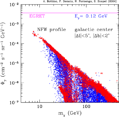
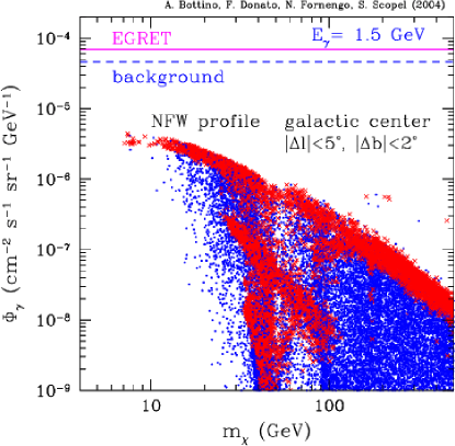
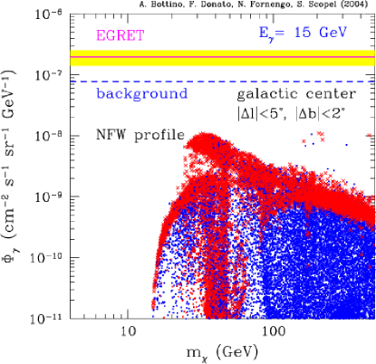
Figure 1: Gamma–ray flux from the galactic center inside the angular region $|\Delta l|\leq 5^{\circ}$, $|\Delta b|\leq 2^{\circ}$ for a NFW matter density profile. The scatter plots are derived by a full scan of the parameter space of the supersymmetric model described in Sec. II. Crosses (red) and dots (blue) denote neutralino configurations with $0.095\leq\Omega_{\chi}h^{2}\leq 0.131$ and $\Omega_{\chi}h^{2}<0.095$, respectively. Top left: flux calculated at $E_{\gamma}=0.12$ GeV; the horizontal line shows the gamma–ray flux measured by EGRET egret_gc , assumed to be compatible with the estimate of the background egret_gc . Top right: flux calculated at $E_{\gamma}=1.5$ GeV; the solid horizontal line shows the gamma–ray flux measured by EGRET egret_gc , the dashed line is an estimate of the gamma–ray background egret_gc . Bottom: flux calculated at $E_{\gamma}=15$ GeV; the solid horizontal line shows the gamma–ray flux measured by EGRET egret_gc , the shaded horizontal band denotes the 1$\sigma$ error bar on the EGRET data and the dashed line is an estimate of the gamma–ray background egret_gc .

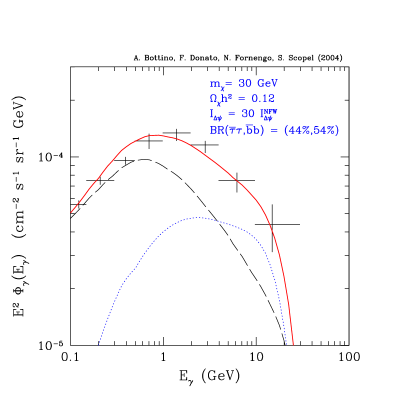
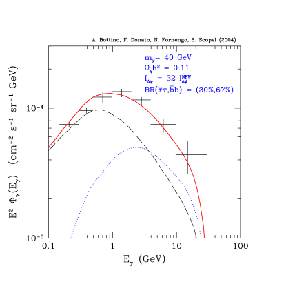
Figure 2: Gamma–ray spectra $\Phi_{\gamma}(E_{\gamma})$, multiplied by $E_{\gamma}^{2}$, from the galactic center inside the angular region $|\Delta l|\leq 5^{\circ}$, $|\Delta b|\leq 2^{\circ}$, as functions of the photon energy. Left panel: the dotted line is the spectrum for a neutralino with mass $m_{\chi}=30$ GeV, calculated for a density profile with a factor 30 of enhancement with respect to the NFW case; the dashed line is the gamma ray background calculated in Ref. egret_gc , reduced by 10%; the solid line is the total flux, sum of the supersymmetric signal and the background; the experimental points are the EGRET data egret_gc . Right panel: the same, for $m_{\chi}=40$ GeV and for a density profile with a factor 32 of enhancement with respect to the NFW case. Both supersymmetric configurations have been selected from the points shown in Fig. 1. The numbers quoted in the legend inside parentheses denote the values of the neutralino annihilation branching ratios into $\bar{b}b$ and $\bar{\tau}\tau$.

Data from low galactic latitudes ($|b|<10^{\circ}$), including the galactic center region, have been collected by the EGRET telescope egret_gc . The diffuse gamma–ray flux of the inner galaxy measured by EGRET shows a possible excess over the estimated background at energies larger than about 1 GeV.

Clearly a firm assessment of an excess requires a good knowledge of the standard production of gamma rays in our Galaxy. At the energies of interest for our analysis - namely, from about 100 MeV to tens of GeV - the main production mechanism of $\gamma$-rays is the interaction of cosmic rays (mainly protons and helium nuclei) with the interstellar medium (atomic and molecular hydrogen, and helium). In these strong reactions $\pi^{0}$’s are produced, and hence $\gamma$-rays via pion decay: $\pi^{0}\rightarrow 2\gamma$. The ensuing spectrum has a bump around 70 MeV, and drops at high energies with an energy power law which follows the progenitor cosmic ray spectrum ($E^{-\alpha}$, with $\alpha\sim$ 2.7). Another source of $\gamma$-rays comes from inverse-Compton scattering of cosmic ray electrons off the interstellar photons. In particular, energetic electrons may scatter off the cosmic microwave background, and off the infrared, optical and ultraviolet radiation arising from stellar activity and dust. The third radiation component originates from electron bremsstrahlung over the interstellar medium, which may be partially or even totally ionized. Bremsstrahlung $\gamma$-rays are mostly important in the low energy tail. For a full calculation of these three main radiation components one needs a good knowledge of the physics of cosmic rays and of the interstellar medium in the region of interest. This is particularly unlikely when dealing with the galactic center area.

In the literature, several different results have been achieved on the subject. First of all, the EGRET Collaboration developed a detailed calculation of the $\gamma$–ray background at the energies of interest for the detector egret_gc ; egret_calc : this calculation shows a clear deficit of $\gamma$-rays towards the GC with respect to measurements. The excess in the data is apparent for $E_{\gamma}\mathrel{\mathop{\kern 0.0pt\hbox to0.0pt{\raise 0.86108pt\hbox{$>$}\hss}}\lower 3.87495pt\hbox{\kern-1.90002pt$\sim$}}1$ GeV, where the shapes of the spectra of the estimated background and the data differ significantly. At lower energies the spectral agreement is instead rather good. Similar conclusions have been drawn in Refs. mori with some different procedure in the calculation of the background. In this paper a harder, probably unrealistic, nucleonic spectrum is shown not to be anyway sufficient to explain the GeV excess. Some modifications towards harder electron and nucleon spectra are studied in Ref. strong , but a satisfactory agreement with data is not achieved (notice that it is anyway hard to reconcile these hypothesis with galactic cosmic rays measurements). The results of all these analyzes favor the interpretation of the EGRET data in terms of an excess over the background, mostly at energies above 1 GeV.

However, different assumptions on acceleration busching and diffusion erlykin of cosmic ray nucleons, and on the spectral shape of primary nucleons in the interstellar space aharonian , have been proposed and lead to a quite good agreement of the EGRET measured flux: almost all the spectral features are reproduced by these calculations. In this case, the EGRET data would be explained in terms of the standard galactic $\gamma$–ray production.

At present, it is very difficult to favor one model against the others, both on theoretical and observational basis. This implies that the uncertainty on the calculation of the galactic $\gamma$-ray flux, and in particular at the galactic center, is very difficult to quantify.

Due to these open problems on the determination of the background component, we will develop our analysis along two paths. First of all we will discuss whether, and under which conditions, it is possible to set constraints on low–mass neutralinos from the gamma-ray studies. Then we will comment on the possibility for low–mass neutralinos to explain the putative EGRET excess.

The gamma–ray flux from the galactic center inside the angular region $|\Delta l|\leq 5^{\circ}$, $|\Delta b|\leq 2^{\circ}$ for a NFW matter density profile is shown in Fig. 1 at three representative photon energies: $E_{\gamma}=$ 0.12, 1.5 and 15 GeV. These energies correspond to three energy bins of the EGRET detector. The scatter plots of the two top panels display a peculiar funnel shape at small masses. This is due to the fact that the neutralino flux is bounded from below by the cosmological limit $\Omega_{\chi}h^{2}\leq(\Omega_{CDM}h^{2})_{\rm max}$. This feature is similar to the one we found in Refs. lowneu ; lowmass ; lowdir , in connection with neutralino direct detection rates. The variation in shape of the scatter plots, when $E_{\gamma}$ is increased, is easily understood in terms of Eq.(4). At $E_{\gamma}=0.12$ GeV the $m_{\chi}^{-2}$ behavior is clearly visible. Energies of the order of 100 MeV are very crucial in offering the possibility to set limits on the very light neutralino sector. By increasing the photon energy, the lightest neutralinos do not have enough phase space to produce photons at this energy (since they annihilate almost at rest in the Galaxy): therefore the gamma–ray flux at very low masses becomes progressively depressed, as $E_{\gamma}$ increases. At $E_{\gamma}=1.5$ GeV a neutralino with a mass of 6 GeV can produce approximately the same flux as a 10-15 GeV neutralino. At $E_{\gamma}=15$ GeV all the neutralinos lighter than 15 GeV obviously do not produce any photon: at this energy the maximal fluxes are obtained for neutralinos with masses around 30 GeV.

The first conclusion which can be drawn from Fig. 1 is that the supersymmetric model considered here is not constrained, at present, by EGRET data for a NFW density profile. An increase in the flux by a factor of 3.3, as would be in the case of the $r$–dependent log–slope profile of Eq.(2), is also not enough to set limits.

Larger enhancements in the geometrical factor $I_{\Delta\psi}$ over the NFW case are necessary to set limits. The comparison of the three panels of Fig. 1 shows that the limits come from different energies $E_{\gamma}$, depending on the neutralino mass. For very light neutralinos, i.e. $m_{\chi}\mathrel{\mathop{\kern 0.0pt\hbox to0.0pt{\raise 0.86108pt\hbox{$<$}\hss}}\lower 3.87495pt\hbox{\kern-1.90002pt$\sim$}}10$ GeV, the lowest energy bin is the relevant one. In this case an enhancement of a factor of 6 would allow to raise the predicted fluxes for $E_{\gamma}=0.12$ GeV at the level of the EGRET measurement, and therefore to start setting limits. For masses in the range $10~{}{\rm GeV}\mathrel{\mathop{\kern 0.0pt\hbox to0.0pt{\raise 0.86108pt\hbox{$<$}\hss}}\lower 3.87495pt\hbox{\kern-1.90002pt$\sim$}}m_{\chi}\mathrel{\mathop{\kern 0.0pt\hbox to0.0pt{\raise 0.86108pt\hbox{$<$}\hss}}\lower 3.87495pt\hbox{\kern-1.90002pt$\sim$}}20~{}{\rm GeV}$ the $E_{\gamma}=1.5$ GeV bin sets more stringent limits, at least on a fraction of the supersymmetric models, but only for a factor of enhancement of at least 15–20 over the NFW case. These factors are pretty large, even though not as large as the one which refers to a Moore et al. profile, which is about 60, as discussed before. For masses around 30–40 GeV the best limits come from the highest energy bin $E_{\gamma}=15$ GeV, where a factor of 20–25 would allow the fluxes to reach the EGRET data. In the case of the standard MSSM, where the neutralino has masses larger than 50 GeV the lowest energy bins are always less constraining that the higher energy ones, as can be seen by comparing the different panels of Fig. 1. Instead, the lower energy bins are crucial for the study of the low–mass neutralinos. We finally comment that a Moore et al. profile would make all the fluxes for $m_{\chi}\mathrel{\mathop{\kern 0.0pt\hbox to0.0pt{\raise 0.86108pt\hbox{$<$}\hss}}\lower 3.87495pt\hbox{\kern-1.90002pt$\sim$}}10$ GeV incompatible with the data, but this profile is less likely, as we discussed above.

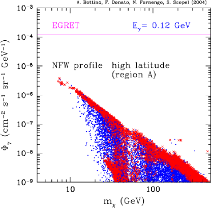
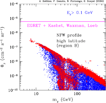
Figure 3: Gamma–ray flux from galactic high–latitudes for a NFW matter density profile. The scatter plots are derived by a full scan of the parameter space of the supersymmetric model described in Sec. II. Crosses (red) and dots (blue) denote neutralino configurations with $0.095\leq\Omega_{\chi}h^{2}\leq 0.131$ and $\Omega_{\chi}h^{2}<0.095$, respectively. Left panel: flux calculated at $E_{\gamma}=0.12$ GeV in the high–latitude regions defined by $|b|>10^{\circ}$ with the exclusion of $|l|\leq 40^{\circ}$ and $10^{\circ}\leq|b|\leq 30^{\circ}$ around the galactic center; the horizontal line shows the gamma–ray residual flux identified by EGRET egret_extragal . Right panel: integrated flux for energies above $E_{\gamma}=0.1$ GeV in the polar regions defined by $|b|\geq 86^{\circ}$; the dashed horizontal line shows the upper limit on a possible residual flux in the polar regions, obtained in Ref. waxman .

Now, let us turn to a brief discussion of the possibility to explain the EGRET excess by means of low–mass neutralinos. The analysis made above on the behavior of the gamma–ray fluxes in the three representative energy bins of Fig. 1 shows that neutralinos in the mass range $25~{}{\rm GeV}\mathrel{\mathop{\kern 0.0pt\hbox to0.0pt{\raise 0.86108pt\hbox{$<$}\hss}}\lower 3.87495pt\hbox{\kern-1.90002pt$\sim$}}m_{\chi}\mathrel{\mathop{\kern 0.0pt\hbox to0.0pt{\raise 0.86108pt\hbox{$<$}\hss}}\lower 3.87495pt\hbox{\kern-1.90002pt$\sim$}}40~{}{\rm GeV}$ are the ones which may have the possibility to fill the excess in the energy range above 1 GeV, without spoiling the lower energy behavior of the background which is supposed to have an acceptable agreement with the data. We show that indeed the low–mass neutralinos in this mass range are able to explain the EGRET excess in Fig. 2. In this figure we plot the predicted gamma–ray spectra for two representative supersymmetric configuration when, for definiteness, the gamma–ray background as calculated in Ref. egret_calc is assumed. In the left panel of Fig. 2 we show a supersymmetric configuration with $m_{\chi}=30$ GeV and a relic abundance in the proper range to explain dark matter: $\Omega_{\chi}h^{2}=0.12$. The dominant annihilation channels of these low–mass neutralinos are $\chi\chi\rightarrow\bar{\tau}\tau$ and $\chi\chi\rightarrow\bar{b}b$ lowneu ; lowmass . Gamma rays coming from annihilation into $\tau$’s give a harder spectrum as compared to the $b$ channel. In this representative point the two channels have (approximately) the same branching ratio: this gives sizable contribution to the gamma–ray flux in all the energy range from 1 to 10 GeV, which is where the excess in the EGRET data is more pronounced. By allowing the background to fluctuate down by 10% and by using a geometrical factor $I_{\Delta\psi}$ 30 times larger than in the NFW case, we show that a pretty good agreement between the total flux and the data can be obtained. We are not quoting a statistical significance for this agreement since we are not performing a systematic statistical analysis here: however, we are interested in showing that, in addition to the standard MSSM neutralinos with masses larger than 50 GeV ullio_morselli , also low–mass neutralinos have the capability of explaining the putative EGRET excess. In both cases, low–mass and standard neutralinos, the values of the line–of–sight integrals $I_{\Delta\psi}$ which are able to explain the EGRET excess are much larger than what is provided by a NFW density profile. However, for neutralinos in the 30–40 GeV mass range these enhancement factors are smaller than in the case of heavier neutralinos, due to the $m_{\chi}^{-2}$ behavior.

The right panel of Fig. 2 shows a second example, with a neutralino of $m_{\chi}=40$ GeV and $\Omega_{\chi}h^{2}=0.11$. The background of Ref. egret_calc is again scaled down by 10%. In this case the geometrical factor is 32 times the NFW one. The branching fraction of annihilation into $b$ quarks is larger than in the previous case. This enhances the contribution to the gamma–ray flux in the 1–3 GeV range without spoiling the agreement at larger energies.

A detailed analysis of the spectral features of the gamma–ray fluxes produced by neutralino annihilation and their comparison with the EGRET data is beyond the scope of the present paper and will be presented elsewhere.

IV.4 Signal from high galactic latitude

Data from high galactic latitudes have been collected by the EGRET telescope egret_extragal . An analysis of the measurements taken over the latitudes $|b|>10^{o}$, and excluding the region $|l|<40^{o}$ and $10^{o}<|b|<30^{o}$ around the galactic center, has been performed in Ref. egret_extragal . All the identified sources as well as the components due to the interactions of cosmic rays with the galactic disk gas have been subtracted egret_extragal . The residual flux, averaged over the considered portion of the sky, has been shown to be isotropic and well fitted by the power law $\Phi_{HL}^{\rm EGRET}(E_{\gamma})=k(E_{\gamma}/E_{0})^{-\alpha}$, where $k=(7.32\pm 0.34)\cdot 10^{-6}$ photons cm^-2 sec^-1 sr^-1 GeV^-1, $\alpha=2.10\pm 0.03$ and $E_{0}=451$ MeV. This spectrum is often referred to as the extragalactic diffuse emission, since no known source inside the Galaxy seems to be responsible for it. One possibility is that it is due to unresolved gamma-ray–emitting blazars. Relying on the analysis by EGRET, one can use the residual flux as an upper bound to any flux due to exotic sources, including annihilation of relic neutralinos. Recently, a re-analysis of EGRET data has been performed in Ref. waxman , taking particular care of the spatial dependence of the observed photons. Working on the integrated flux and taking into account contributions from several galactic tracers, the authors of Ref. waxman show that the high-latitude $\gamma$-ray sky exhibits strong galactic features and could be well accommodated by simple galactic models. Conservative constraints have been set on the flux integrated above 100 MeV and averaged over different sectors of the sky far from the galactic plane. In this scenario, the room left to an unexplained diffuse flux – often considered as an extragalactic background, but also possibly due to exotic galactic sources – is much smaller (by a factor of three, at least) than the one reported in Ref. egret_extragal . Here we consider the upper limit of Ref. waxman on this possible residual, isotropic flux $I_{\gamma}$ in the polar region ($|b|>86^{0}$): $I_{\gamma}<0.6\cdot 10^{-5}$ $\gamma\;{\rm sec}^{-1}{\rm cm}^{-2}{\rm sr}^{-1}$, and compare it to our estimates for the $\gamma$-ray flux due to neutralino annihilation averaged in the same spatial region.

The results for both estimates are shown in Fig. 3 for a NFW profile. As in the case of the galactic center emission, also for high latitudes we do not have constraints on the supersymmetric parameter space. Contrary to the case of the galactic center region, for high latitudes the geometrical factor $I_{\Delta\psi}$ is practically independent of the halo profile, as discussed before. We therefore conclude that at present the $\gamma$–ray signals from high galactic latitudes do not provide any constraint on the supersymmetric parameter space. The situation could change if further studies will show that a much bigger fraction of the EGRET measured flux at high latitudes is due to galactic foreground or when next–generation experiments will provide further information.

V Antiprotons in cosmic rays

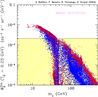
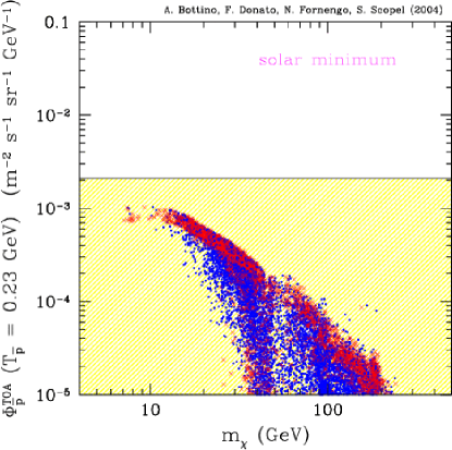
Figure 4: Antiproton flux at $T_{\bar{p}}=0.23$ GeV as a function of the neutralino mass, calculated at solar minimum. The scatter plots are derived by a full scan of the parameter space of the supersymmetric model described in Sec. II. A spherical isothermal dark matter density profile has been used. The solar modulation is calculated at the phase of solar minimum. Crosses (red) and dots (blue) denote neutralino configurations with $0.095\leq\Omega_{\chi}h^{2}\leq 0.131$ and $\Omega_{\chi}h^{2}<0.095$, respectively. The shaded region denotes the amount of primary antiprotons which can be accommodated at $T_{\bar{p}}=0.23$ GeV without entering in conflict with the experimental BESS data bess95-97 ; bess98 and secondary antiproton calculations pbar_sec . Left panel: the best fit set for the astrophysical parameters is used. Right panel: the astrophysical parameters which provide the most conservative antiproton fluxes are used.

Like in the case of the gamma–ray flux, the production of antiprotons from neutralino annihilation results from the hadronization of quarks and gluons created in the annihilation process pbar_history ; pbar0 ; Bottino_Salati ; bergstrom ; pbar_susy . The differential rate per single annihilation, unit volume and time is defined as:

$$q_{\bar{p}}^{\rm susy}(r,T_{\bar{p}})=\,\langle\sigma_{\rm ann}v\rangle\,\frac{dN_{\bar{p}}}{dT_{\bar{p}}}\frac{1}{2}\left(\frac{\rho_{\chi}(r)}{m_{\chi}}\right)^{2},$$ (8)

where $T_{\bar{p}}$ denotes the antiproton kinetic energy, $dN_{\bar{p}}/dT_{\bar{p}}$ (indicated as $g(T_{\bar{p}})$ in Refs.Bottino_Salati ; pbar_susy ) is the differential antiproton spectrum per annihilation event, and the factor 1/2 accounts for the number of annihilating neutralino pairs. The spectrum $dN_{\bar{p}}/dT_{\bar{p}}$ is evaluated by means of the Monte Carlo simulations we already used in Sec. IV.1.

Once antiprotons are produced in the dark halo, they diffuse and propagate throughout the Galaxy. To describe these processes, we follow the treatment of Ref. pbar_susy , to which we refer for details. Here we only recall that the propagation of antiprotons has been considered in a two-zone diffusion model PaperI ; PaperI_bis ; revue , defined in terms of six free parameters whose role is to take into account the main physical processes which affect the propagation of cosmic rays in the Galaxy: acceleration of primary nuclei, diffusion, convective wind, reacceleration process and interaction with the interstellar medium. These free parameters are constrained by comparing the fluxes of various cosmic ray species calculated in our diffusion model with observations. In this regard, the most important observable is the measured Boron/Carbon ratio ($B/C$), whose analysis within our diffusion model is presented in Ref. PaperI_bis . The parameters constrained by the $B/C$ measurements have been shown to be compatible with a series of other observed species PaperI_bis ; pbar_sec ; beta_rad , further supporting the employed model. Therefore, in the calculation of the primary antiproton flux we only use those values for the propagation parameters which provide a good statistical agreement to the $B/C$ data. One of the main results obtained in Ref. pbar_susy is that the supersymmetric antiproton flux, when calculated with the selected propagation parameters, is affected by a large uncertainty. At low energy this uncertainty reaches almost two orders of magnitude, while it diminishes to a factor of thirty at higher energies. Only better and more complete data on cosmic rays (both stable and radioactive) could help in reducing this uncertainty.

At variance with the gamma ray signal, the supersymmetric antiproton flux measured at Earth is almost insensitive to the specific form of the dark matter distribution function, among those discussed in Sec. III. Indeed, these various distributions differ mainly at the galactic center, while at solar neighborhood differences are very mild. Since charged particles, such as antiprotons, suffer enormous energy redistributions, gains and losses, it is almost impossible for an antiproton produced around the galactic center to reach the Earth. This property was shown in Ref. origin , and quantified in Ref. pbar_susy for the case of a NFW distribution and an isothermal one.

In the present work, we use directly the results reached in Ref. pbar_susy , where the function

$$C^{\rm prop}_{\rm susy}(T_{\bar{p}})=\frac{\Phi_{\bar{p}}(r_{\odot},T_{\bar{p}})}{\Upsilon g(T_{\bar{p}})}$$ (9)

was calculated. In this equation, $\Phi_{\bar{p}}(r_{\odot},T_{\bar{p}})$ is the interstellar antiproton flux after propagation and $\Upsilon$ is the supersymmetric flux factor:

$$\Upsilon=\frac{1}{2}\xi^{2}\,\frac{\langle\sigma_{\rm ann}v\rangle}{m_{\chi}^{2}}.$$ (10)

The quantity $C^{\rm prop}_{\rm susy}(T_{\bar{p}})$ may be considered as a measure of how the source flux $q_{\bar{p}}^{\rm susy}(r,T_{\bar{p}})$ is modified by the propagation of antiprotons in the Galaxy before reaching the heliosphere. In the results presented in the following, we have calculated the antiproton flux $\Phi_{\bar{p}}(r_{\odot},T_{\bar{p}})$ according to Eq. (9), where the $C^{\rm prop}_{\rm susy}(T_{\bar{p}})$ function has been taken directly from Ref. pbar_susy for a few representative combinations of the propagation parameters and source spectra $g(T_{\bar{p}})$. We have calculated the quantities entering the factor $\Upsilon$ as described in Sec. II.

V.1 Secondary antiprotons

Antiprotons in the Galaxy are also produced via standard interactions. Proton and helium cosmic rays interact with the interstellar hydrogen and helium nuclei, producing quarks and gluons that subsequently can hadronize into antiprotons. A calculation of this secondary antiproton flux has been done in Ref. pbar_sec , to which we refer for details. Here we only emphasize the main results obtained in that work: i) The antiproton flux has been evaluated consistently by employing the propagation parameters as derived from a full and systematic analysis on stable nuclei PaperI ; ii) This secondary antiproton flux is in very good agreement with the data taken from the experiments bess bess95-97 ; bess98 , ams ams98 , caprice caprice (see Fig. 14 in Ref. pbar_susy ); iii) The uncertainty on the final flux due to propagation is about 20%, with a slight dependence on the energy. Another important source of uncertainty of order 20%-25% resides in the nuclear production cross sections, in particular when considering the interactions over the interstellar helium.

V.2 Constraints on a primary antiproton source?

As discussed above, the secondary antiproton flux already provides a satisfactory agreement with current experimental data, and then no much room is left to primary contributions. This situation suggests that antiproton data could be used to place significant constraints on supersymmetric parameters. However, one has to notice that, as shown in pbar_susy , the supersymmetric primary flux is affected by uncertainties much larger than those related to the secondary flux. This is due to the fact that the sources of the latter are located in the galactic disk. On the contrary, the relic neutralinos are expected to be distributed in the whole galactic halo and then produce an antiproton flux much more sensitive to the astrophysical parameters.

To show quantitatively how the experimental data could constrain the supersymmetric parameters, in Fig. 4 we display the antiproton flux evaluated at $T_{\bar{p}}=0.23$ GeV for a full scan of our supersymmetric model described in Sec. II. As expected, the scatter plot is prominent at small masses. Furthermore, it is remarkable that for $m_{\chi}\mathrel{\mathop{\kern 0.0pt\hbox to0.0pt{\raise 0.86108pt\hbox{$<$}\hss}}\lower 3.87495pt\hbox{\kern-1.90002pt$\sim$}}$ 25 GeV the scatter plot is funnel-shaped. The reason is the same as the one given above in connection with Fig. 1. The two panels of Fig. 4 correspond to two different sets of the propagation parameters. One, used in the left panel, is the set giving the best fit to the $B/C$ ratio, while the other, hereby denoted as the conservative set and used in the right panel provides the lowest (secondary and primary) antiproton fluxes. A spherical cored isothermal distribution for dark matter has been used. However, as mentioned before, a different choice does not significantly modifies the scatter plots. The shaded region denotes the amount of primary antiprotons which can be accommodated at $T_{\bar{p}}=0.23$ GeV without entering in conflict with the BESS experimental data bess95-97 ; bess98 and secondary antiproton calculations pbar_sec .

From the right panel of Fig. 4 we conclude that, within the current astrophysical uncertainties, one cannot derive any constraint on the supersymmetric parameters, if one assumes a very conservative attitude in the selection of the propagation parameters. It is worth noticing that even within this choice, some supersymmetric configurations at very small masses are close to the level of detectability. As a further comment on the left panel of Fig. 4, we wish to stress that any further breakthrough in the knowledge of the astrophysical parameters would allow a significant exploration of small mass configurations, in case the conservative set of parameters is excluded. Should the effect of antiproton propagation turn out to be equivalent to the one obtained with the best fit set, the analysis of cosmic antiprotons would prove quite important for exploring very light neutralinos. This is particularly true for neutralino masses below $\mathrel{\mathop{\kern 0.0pt\hbox to0.0pt{\raise 0.86108pt\hbox{$<$}\hss}}\lower 3.87495pt\hbox{\kern-1.90002pt$\sim$}}$ 15 GeV, in view of the typical funnel shape displayed in the scatter plots.

VI Upgoing muons at neutrino telescopes

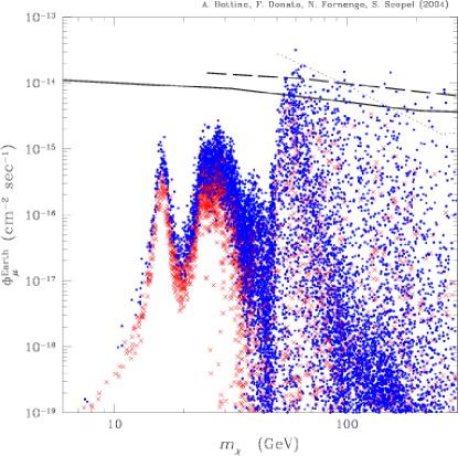
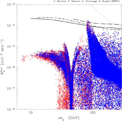
Figure 5: Flux of upgoing muons as a function of the neutralino mass. The scatter plots are derived by a full scan of the parameter space of the supersymmetric model described in Sec. II. Crosses (red) and dots (blue) denote neutralino configurations with $0.095\leq\Omega_{\chi}h^{2}\leq 0.131$ and $\Omega_{\chi}h^{2}<0.095$, respectively. Left panel: signal from the Earth; the solid, dashed and dotted lines denote the experimental upper limits from SuperKamiokande sk , MACRO macro and AMANDA amanda , respectively. Right panel: signal from the Sun; the solid, dashed, dot-dashed and dotted lines denote the experimental upper limits from SuperKamiokande sk , MACRO macro , Baksan baksan and AMANDA amanda , respectively.

Indirect evidence for WIMPs in our halo may be obtained at neutrino telescopes by measurements of the upgoing muons, which would be generated by neutrinos produced by pair annihilation of neutralinos captured and accumulated inside the Earth and the Sun others_mu ; noi_mu . The process goes through the following steps: capture by the celestial body of the relic neutralinos through a slow–down process due essentially to neutralino elastic scattering off the nuclei of the macroscopic body; accumulation of the captured neutralinos in the central part of the celestial body; neutralino–neutralino annihilation with emission of neutrinos; propagation of neutrinos (we have included the $\nu_{\mu}$–$\nu_{\tau}$ vacuum oscillation effect with parameters: $\Delta m^{2}=3\times 10^{-3}$ eV², $\sin\theta=1$) and conversion of their $\nu_{\mu}$ component into muons in the rock surrounding the detector; propagation and detection of the ensuing upgoing muons in the detector.

The various quantities relevant for the previous steps are calculated here according to the method described in Refs. noi_mu , to which we refer for further details. We just recall that the neutrino flux due to the annihilation processes taking place in a distant source like the Sun, as a function of the neutrino energy $E_{\nu}$, is given by

$$\frac{dN_{\nu}}{dE_{\nu}}=\frac{\Gamma_{A}}{4\pi d^{\,2}}\sum_{F,f}B^{(F)}_{\chi f}\frac{dN_{f\nu}}{dE_{\nu}},$$ (11)

where $\Gamma_{A}$ is the annihilation rate inside the macroscopic body griest , $d$ is the distance from the source, $F$ denotes the $\chi$–$\chi$ annihilation final states, $B^{(F)}_{\chi f}$ denotes the branching ratios into heavy quarks, $\tau$ leptons and gluons in the channel $F$; $dN_{f\nu}/dE_{\nu}$ is the differential distribution of the neutrinos generated by the hadronization of quarks and gluons and the subsequent hadronic semileptonic decays. The annihilation rate is given by $\Gamma_{A}=C/2~{}{\rm tanh}^{2}(t_{0}/\tau_{A})$ griest , where $t_{0}$ is the age of the macroscopic body, $\tau_{A}=(CC_{A})^{-1/2}$, $C_{A}$ is the annihilation rate proportional to the neutralino–neutralino annihilation cross–section and $C$ denotes the capture rate per effective volume of the body. The capture rate $C$ is calculated here as in Refs. gould ; helio , the WIMP velocity distribution in the galactic inertial frame being described by a Maxwellian function with a dispersion velocity of 270 km s^-1. We recall that the capture rate by the Earth is favored when the WIMP mass is close to the nuclear mass of one of the main chemical components of the Earth: Oxygen, Magnesium, Silicon in the mantle and Iron in the core gould . We have neglected the contributions of the light quarks directly produced in the annihilation process or in the hadronization of heavy quarks and gluons, because these light particles stop inside the medium (Sun or Earth) before their decay. For the case of the Sun we have also considered the energy loss of the heavy hadrons in the solar medium.

VI.1 Neutrinos from the center of the Earth

In the left panel of Fig. 5 we show the expected upgoing muon flux integrated for $E_{\mu}>$1 GeV, as a function of $m_{\chi}$, and compared to the present experimental upper bounds on the same quantity from the experiments Superkamiokande sk , MACRO macro , and AMANDA amanda . For $m_{\chi}\mathrel{\mathop{\kern 0.0pt\hbox to0.0pt{\raise 0.86108pt\hbox{$<$}\hss}}\lower 3.87495pt\hbox{\kern-1.90002pt$\sim$}}$ 40 GeV the signal from the Earth presents several peaks due to resonant capture on Oxygen, Silicon and Magnesium (we recall that the process of capture on Earth is driven by the coherent neutralino–nucleus cross section). These elements are almost as abundant in Earth as Iron, which is the most important target nucleus for neutralino capture at higher masses. The dip at $m_{\chi}\simeq M_{Z}/2$ is due to the rescaling prescription of Eq. (3), since the resonance in the $Z$–exchange annihilation cross section reduces the relic abundance $\Omega_{\chi}h^{2}$. Moreover, for $m_{\chi}\mathrel{\mathop{\kern 0.0pt\hbox to0.0pt{\raise 0.86108pt\hbox{$<$}\hss}}\lower 3.87495pt\hbox{\kern-1.90002pt$\sim$}}$ 25 GeV, the branching ratio $B^{(\tilde{\tau})}_{\chi\tau}$ to the $\tau\bar{\tau}$ final state, which is the one with the highest neutrino yield per annihilation, is suppressed. This last property is due to the fact that, in this range of $m_{\chi}$, the final state to $b\bar{b}$ in the annihilation cross section is required to be the dominant one in order to keep the relic abundance $\Omega_{\chi}h^{2}$ below its cosmological upper bound lowmass . This, together with the fact that lower $\chi$ masses imply softer $\nu$ spectra that produce less $\mu$’s above threshold, explains why the up-going muon signal expected for light neutralinos ($m_{\chi}\mathrel{\mathop{\kern 0.0pt\hbox to0.0pt{\raise 0.86108pt\hbox{$<$}\hss}}\lower 3.87495pt\hbox{\kern-1.90002pt$\sim$}}$ 50 GeV) turns out to be below the level reached at higher masses.

It is worth noting that substantial modifications to the standard Maxwellian velocity distribution in the solar neighborhood have been considered in recent years, with two conflicting models. Damour and Krauss dk proposed the existence of a solar-bound population, generated by WIMPs which scattered off the Sun surface and were then set, by perturbations from other planets, into orbits crossing the Earth, but not the Sun. The existence of this low-speed population would make the capture of WIMPs by the Earth very efficient with an ensuing dramatic enhancement of the up-going muon flux as compared to the standard case bdeku . On the contrary, Gould and Alam ga used arguments based on calculations of asteroid trajectories to conclude that solar-bound WIMPs could evolve quite differently, inducing a significant suppression in the up-going muon flux from the Earth, as compared to the standard Maxwellian case, for WIMP masses larger than 150 GeV. A very recent re–analysis of this problem le supports the conclusions of Gould and Alam, though with a less dramatic suppression effect. Our results have been derived using the standard Maxwellian distribution. The results of Ref. le would not significantly alter our conclusion on the detectability of light neutralinos. The maximal fluxes are obtained for resonant capture on $O$, $Si$ and $Mg$ nuclei in the mantle: in this situation no suppression occurs. For neutralino masses away from the resonant condition, a reduction factor up to 0.8 for $m_{O}\mathrel{\mathop{\kern 0.0pt\hbox to0.0pt{\raise 0.86108pt\hbox{$<$}\hss}}\lower 3.87495pt\hbox{\kern-1.90002pt$\sim$}}m_{\chi}\mathrel{\mathop{\kern 0.0pt\hbox to0.0pt{\raise 0.86108pt\hbox{$<$}\hss}}\lower 3.87495pt\hbox{\kern-1.90002pt$\sim$}}m_{Fe}$ and up to 2–3 for $m_{\chi}\mathrel{\mathop{\kern 0.0pt\hbox to0.0pt{\raise 0.86108pt\hbox{$<$}\hss}}\lower 3.87495pt\hbox{\kern-1.90002pt$\sim$}}10$ GeV is possible le : however, in these cases, the upgoing muon flux is already very depressed, as it is shown in Fig. 5, left panel. In conclusion, using the standard Maxwellian distribution, the present measurements of up-going muons from the Earth put some constraints on neutralino configurations for masses above 50 GeV. For lighter neutralinos, explorations by neutrino telescopes would require a substantial increase in sensitivity while keeping a low energy threshold (close to 1 GeV). This in turn would imply a sizable extension of the telescope and a dense array of photomultipliers, which is certainly feasible, but very expensive.

VI.2 Neutrinos from the Sun

In the right panel of Fig. 5 we show the up-going muon flux expected from the Sun, integrated for $E_{\mu}>$1 GeV, as a function of $m_{\chi}$. The signal is compared to the present experimental upper bounds on this flux coming from the experiments Superkamiokandesk , MACROmacro , AMANDAamanda and Baksanbaksan . Also in this case the signal level turns out to be suppressed for $m_{\chi}\mathrel{\mathop{\kern 0.0pt\hbox to0.0pt{\raise 0.86108pt\hbox{$<$}\hss}}\lower 3.87495pt\hbox{\kern-1.90002pt$\sim$}}$ 50 GeV as compared to what is obtained at higher masses, the reasons of this behavior being the same as in the case of the Earth. On the other hand, the enhancement of the signal at $m_{\chi}\sim m_{W}$ is due to a peculiar behavior of the neutralino–nucleon spin–dependent cross section, which drives the neutralino capture in the Sun (mainly on hydrogen). This cross section reaches its maximum whenever the $Z$–exchange channel dominates, and this requirement is verified when the neutralino–$Z$ coupling, proportional to the combination $a_{3}^{2}-a_{4}^{2}$, is maximal spin . By numerical inspection we have verified that this last quantity is significantly peaked for $m_{\chi}\sim M_{W}$. In this range of masses the annihilation channel to $W^{+}W^{-}$ opens up and dominates the annihilation cross section. We conclude here that investigations of light neutralinos by up-going muons from the Sun do not provide favourable prospects.

VII Conclusions and Perspectives

We have considered the most relevant indirect strategies for detecting the presence of relic neutralinos in our Galaxy through the products of their self-annihilation. This includes annihilations taking place directly in the galactic halo or inside celestial bodies (Earth and Sun). Our investigation has been performed in the frame of an effective supersymmetric model at the electroweak scale with no assumption on gaugino mass universality at the GUT scale. The range of the neutralino mass taken into consideration brackets a wide interval, from 6 GeV up to 500 GeV. While the low extreme is decided by the lower bound of 6 GeV, established in Ref. lowneu ; lowmass , the upper extreme of 500 GeV is chosen only for convenience. Actually, no model-independent upper limit for the neutralino mass is available, apart for a generic value of order of 1 TeV, beyond which the raison d’être of supersymmetry fades away. Though our calculations span over the wide range of the neutralino masses recalled above, our discussions were focused on light neutralinos, i.e. neutralinos with masses below 50 GeV: this value corresponds to the lower bound of $m_{\chi}$ when gaugino-mass unification is assumed. Indeed, light neutralinos are rarely considered in the literature, though their properties are quite interesting, as we already proved in connection with their cosmological properties and their detectability by current experiments of direct WIMP search lowneu ; lowmass ; lowdir . Thus the present paper is the natural continuation of our previous investigations on neutralinos of small mass. Different galactic dark matter distributions have been considered, from the cored isothermal one to the profiles obtained by numerical cosmological simulations in Refs. nfw ; moore , including also the most recent ones of Ref. navarro .

Now we summarize the main results of the present paper:

• For the $\gamma$ rays we have considered separately fluxes from the galactic center and high latitude regions, and compared our predictions with the EGRET data. Our numerical results have been provided employing as a reference DM distribution the NFW profile. We have shown that in this case the EGRET data at all angles do not put any constraints on the supersymmetric flux. The minimum gap between the theoretical predictions and the data occurs at light masses and is of almost one order of magnitude. We have discussed by how much this gap changes in terms of the dark matter distribution. This variation is relevant only for signals coming from the galactic center. For this sector, we have shown that using the $r$–dependent log–slope distribution of Ref. navarro the gap between data and supersymmetric fluxes is reduced by a factor of 3 with respect to the NFW profile. Only profiles as steep as the Moore et al. one, disfavored by recent simulations, could exclude some light neutralino configurations. We have also shown that neutralinos of masses around 30–40 GeV could explain the EGRET excess in case of a significant enhancement effect as compared to the NFW distribution. A general word of caution concerns the fact that the background due to conventional cosmic rays production mechanisms still suffers from sizeable uncertainties.

• We have shown that in the case of cosmic antiprotons, no constraint on the supersymmetric parameters can be derived, if one assumes a very conservative attitude in the selection of the propagation parameters. However, it is remarkable that indeed the signal at very small masses is close to the level of detectability. Some breakthrough in the knowledge of the astrophysical parameters could allow a significant exploration of small mass configurations. This is particularly true for neutralino masses below about 15 GeV, in view of the typical funnel shape displayed in the scatter plots.

• The present measurements of up-going muons from the center of the Earth put some constraints on neutralino configurations for masses above 50 GeV. For lighter neutralinos, explorations by neutrino telescopes require a substantial increase in sensitivity with an energy threshold close to 1 GeV. Investigations of light neutralinos by up-going muons from the Sun are very disfavored.

We wish to recall that, according to the measurements of the HEAT Collaboration heat , the spectrum of the positron component of cosmic rays shows some enhancement between 7 and 20 GeV. This is only a mild effect which, as shown in Ref. heat , could be explained in terms of conventional secondary production mechanisms. Alternatively, some authors have interpreted this effect as a deviation from a pure secondary flux, which could be generated by neutralino self-annihilation kane ; be . This hypothesis, to be a viable one, requires that the neutralino flux is enhanced by a sizable factor. Since the measured positrons must be created in a region around the Earth of a radius of a few kpc origin , an enhancement would imply a significant dark matter overdensity in that region, with implications for the $\bar{p}$ signal. This scenario appears strongly model dependent, and as such not suitable for setting constraints to supersymmetric parameters.

Antideuterons in space as a signal of neutralino self-annihilation, which were shown in Ref.dbar to be a very promising investigation means, will be considered in a forthcoming paper.

- (1) A. Bottino, N. Fornengo and S. Scopel, Phys. Rev. D 67, 063519 (2003) [hep-ph/0212379].
- (2) A. Bottino, F. Donato, N. Fornengo and S. Scopel, Phys. Rev. D 68, 043506 (2003) [hep-ph/0304080].
- (3) A. Bottino, F. Donato, N. Fornengo and S. Scopel, Phys. Rev. D 69, 037302 (2004) [hep-ph/0307303].
- (4) For prospects to detect these light neutralinos at tevatron and colliders see: G. Bélanger, F. Boudjema, A. Cottrant, A. Pukhov, S. Rosier-Lees, hep-ph/0310037.
- (5) S. Ahmed et al., (CLEO Collaboration), CONF 99/10, arXiv:hep-ex/9908022; R. Barate et al. (ALEPH Collaboration), Phys. Lett. B 429, 169 (1998); K. Abe et al. (Belle Collaboration), Phys. Lett. B 511, 151 (2001).
- (6) D. Acosta et al., (CDF Collaboration), hep-ex/0403032.
- (7) C. Bobeth, T. Ewerth, F. Krüger and J. Urban, Phys. Rev. D 64, 074014 (2001); A. Dedes, H. K. Dreiner and U. Nierste, Phys. Rev. Lett. 87, 251804 (2001).
- (8) M. Carena, D. Garcia, U. Nierste and C.E.M. Wagner, Phys. Lett. B 499, 141 (2001) and references quoted therein.
- (9) M. Davier et al., Eur.Phys.J. C 31, 503 (2003).
- (10) K. Hagiwara et al., hep-ph/0312250.
- (11) D.N. Spergel et al., Astrophys. J. Suppl. 148, 175 (2003).
- (12) M. Tegmark et al., in press on Pyhs. Rev. D, astro-ph/0310723.
- (13) A. Bottino, V. de Alfaro, N. Fornengo, G. Mignola, and M. Pignone, Astropart. Phys. 2, 67 (1994).
- (14) L. Hernquist, Astrophys. J. 356, 359 (1990).
- (15) F. Eisenhauer et al., Astrophys. J. 597, L121 (2003).
- (16) J.F. Navarro, C.S. Frenk and S.D.M. White, Astrophys. J. 462, 563 (1996).
- (17) B. Moore et al., Mon. Not. Roy. Astron. Soc. 310, 1147 (1999).
- (18) J. F. Navarro et al., to appear in Mon. Not. Roy. Astron. Soc., astro-ph/0311231.
- (19) See, for instance, A. Borriello and P. Salucci, Mont. Not. R. Astron. Soc. 232 (2001) 285.
- (20) P. Belli, R. Cerulli, N. Fornengo and S. Scopel, Phys. Rev. D 66, 043503 (2002) and references therein.
- (21) H. Bengtsson, P. Salati and J. Silk, Nucl. Phys. B 346, 129 (1990).
- (22) J. Silk and A. Stebbins, Astrophys. J. 411, 439 (1993).
- (23) V. Berezinsky, A. Bottino and G. Mignola, Phys. Lett. B 391, 355 (1997).
- (24) L. Bergström, J. Edsjö, and P. Ullio, Phys. Rev. D 58, 083507 (1998); L. Bergström, J. Edsjö, P. Gondolo, and P. Ullio, Phys. Rev. D 59, 043506 (1998);
- (25) R. Aloisio, P. Blasi, and A. V. Olinto, astro-ph/0206036; B. Moore et al., Astrophys. J 524, L19 (1999).
- (26) V. Berezinsky, V. Dokuchaev and Yu. Eroshenko, Phys. Rev. D 68, 103003 (2003).
- (27) F. Stoher et al., Mon. Not. Roy. Astron. Soc. 345, 1313 (2003).
- (28) V. Berezinsky, A. Bottino, G. Mignola, Phys. Lett. B325, 136 (1994); G. Jungman, M. Kamionkowsky, Phys. Rev. D 51, 3121 (1995); P. Chardonnet et al., Ap. J 454, 774 (1995); L. Bergström, P. Ullio and J. Buckley, Astropart. Phys. 9, 137 (1998); P. Ullio and L. Bergström, Nucl. Phys. B504, 27 (1997); Phys. Rev. D 57, 1962 (1998); S. Peirani, P. Mohayaee, J.A. de Freitas Pacheco, astro-ph/0401378.
- (29) P. Ullio, L. Bergström, J. Edsjö and C. Lacey, Phys. Rev. D 66, 123502 (2002).
- (30) T. Sjöstrand, P. Eden, C. Friberg, L. Lonnblad, G. Miu, S. Mrenna and E. Norrbin, Comput. Phys. Commun. 135, 238 (2001).
- (31) More details about our evaluation of the spectrum from neutralino self–annihilations will be presented in a separate paper.
- (32) F. Donato, N. Fornengo, D. Maurin, P. Salati, R. Taillet in press on Phys. Rev. D, astro-ph/0306207.
- (33) S.D. Hunter et al., Astrophys. J. 481, 205 (1997).
- (34) P. Sreekumar et al., Astrophys. J. 494, 523 (1998).
- (35) U. Keshet, E. Waxman and A. Loeb, subm. to Astrophys. J., astro-ph/0306442.
- (36) H.A. Mayer-Hasselwander et al., Astron. & Astrophys. 335, 161 (1998).
- (37) D.L. Bertsch et al., Astrophys. J. 416, 587 (1993).
- (38) M. Mori, Astrophys. J. 478, 225 (1997).
- (39) A.W. Strong, I.V. Moskalenko and O. Reimer, Astrophys. J. 537, 763 (2000).
- (40) I. Büsching, M. Pohl, and R. Schlickeiser, Astron. & Astrophys. 377, 1056 (2001).
- (41) A.D. Erlykin and A.W.Wolfendale, J. Phys. G: Nucl. Part. Phys. 28, 2329 (2002).
- (42) F.A. Aharonian and A.M. Atoyan, Astron. & Astrophys. 362, 937 (2000).
- (43) A. Cesarini et al., astro-ph/0305075.
- (44) J. Silk and M. Srednicki, Phys. Rev. Lett. 53, 624 (1984); J. Ellis, R.A. Flores, K. Freese, S. Ritz, D. Seckel and J. Silk, Phys. Lett. B 214, 403 (1988); F. Stecker, S. Rudaz and T. Walsch, Phys. Rev. Lett. 55, 2622 (1985); J.S. Hagelin and G.L. Kane, Nucl. Phys. B 263, 399 (1986); S. Rudaz and F.W. Stecker, Astrophys. J. 325, 16 (1988); F. Stecker and A. Tylka, Astrophys. J. 336, L51 (1989); G. Jungman and M. Kamionkowski, Phys. Rev. D 49, 2316 (1994).
- (45) A. Bottino, C. Favero, N. Fornengo, and G. Mignola, Astropart. Phys. 3, 77 (1995).
- (46) A. Bottino, F. Donato, N. Fornengo, and P. Salati, Phys. Rev. D 58, 123503 (1998).
- (47) L. Bergström, J. Edsjö, and P. Ullio, Astrophys. J. 526, 215 (1999).
- (48) D. Maurin, F. Donato, R. Taillet, and P. Salati, Astrophys. J. 555, 585 (2001).
- (49) D. Maurin, R. Taillet, F. Donato, Astron. & Astrophys. 394, 1039 (2002).
- (50) D. Maurin, R. Taillet, F. Donato, P. Salati, A. Barrau, and G. Boudoul, in Research Signposts, “Recent Developments in Astrophysics”, astro-ph/0212111.
- (51) F. Donato et al., Astrophys. J. 563, 172 (2001).
- (52) F. Donato, D. Maurin, and R. Taillet, Astron. & Astrophys. 381, 539 (2002).
- (53) D. Maurin and R. Taillet, Astron. & Astrophys. 404, 949 (2003).
- (54) S. Orito, et al. (BESS Collaboration), Phys. Rev. Lett. 84, 1078 (2000).
- (55) T. Maeno, et al. (BESS Collaboration), Astropart. Phys. 16, 121 (2001).
- (56) M Aguilar, et al. (AMS Collaboration), Phys. Rep. 366, 331 (2002).
- (57) M. Boezio, et al. (CAPRICE Collaboration), Astrophys. J. 561, 787 (2001).
- (58) J. Silk, K. Olive and M. Srednicki, Phys. Rev. Lett. 55, 257 (1985); T. Gaisser, G. Steigman and S. Tilav, Phys. Rev. D 34, 2206 (1986); K. Freese, Phys. Lett. B 167, 295 (1986); K. Griest and S. Seckel, Nucl. Phys. B 279, 804 (1987); G.F. Giudice and E. Roulet, Nucl. Phys. B 316 (1989) 429; G.B. Gelmini, P. Gondolo and E. Roulet, Nucl. Phys. B 351, 623 (1991); M. Kamionkowski, Phys. Rev. D 44, 3021 (1991); F. Halzen, M. Kamionkowski and T. Steltzer, Phys. Rev. D 45, 4439 (1992); M. Mori et al., Phys. Rev. D 48, 5505 (1993); M. Drees, G. Jungman, M. Kamionkowski and M.M. Nojiri, Phys. Rev. D 49, 636 (1994); R. Gandhi, J.L. Lopez, D.V. Nanopoulos, K. Yuan and A. Zichichi, Phys. Rev. D 49, 3691 (1994); L. Bergström, J. Edsjö and P. Gondolo, Phys. Rev. D 55, 1765 (1997); L. Bergström, J. Edsjö and M. Kamionkowski, Astrop. Phys. 7, 147 (1997).
- (59) A. Bottino, V. de Alfaro, N. Fornengo, G. Mignola and M. Pignone, Phys. Lett. B 265, 57 (1991); A. Bottino, N. Fornengo, G. Mignola and L. Moscoso, Astroparticle Physics 3, 65 (1995); V. Berezinsky, A. Bottino, J. Ellis, N. Fornengo, G. Mignola and S. Scopel, Astrop. Phys. 5, 333 (1996); A. Bottino, F. Donato, N. Fornengo and S. Scopel, Astropart. Phys. 10, 203 (1999); A. Bottino, F. Donato, N. Fornengo and S. Scopel, Phys. Rev. D 62, 056006 (2000).
- (60) K. Griest and D. Seckel, Nucl. Phys. B 283, 681 (1987).
- (61) A. Gould, Astrophys. J. 321, 571 (1987); 368, 610 (1991).
- (62) A. Bottino, G. Fiorentini, N. Fornengo, B. Ricci, S. Scopel, F.L. Villante Phys. Rev. D 66, 053005 (2002).
- (63) A. Habig [Super-Kamiokande Collaboration], hep-ex/0106024.
- (64) M. Ambrosio et al. [MACRO Collaboration], Phys. Rev. D 60, 082002 (1999).
- (65) X. Bai et al. (AMANDA Collaboration), Proceedings of the 28th International Cosmic Ray Conferences (ICRC 2003), Tsukuba, Japan, 31 Jul - 7 Aug 2003.
- (66) T. Damour and L.M. Krauss, Phys. Rev. Lett. 81, 5726 (1998); Phys. Rev. D 59, 063509 (1999).
- (67) L. Bergström, T. Damour, J. Edsjö, L.M. Krauss and P. Ullio, JHEP 09, 999 (1999).
- (68) A. Gould and S.M.K. Alam, Astrophys. J. 549, 72 (2001).
- (69) J. Lundberg and J Edsjö, astro-ph/0401113.
- (70) M. M. Boliev et al., Prepared for International Workshop on Aspects of Dark Matter in Astrophysics and Particle Physics, Heidelberg, Germany, 16-20 Sep 1996.
- (71) A. Bottino, F. Donato, G. Mignola, S. Scopel, P. Belli and A. Incicchitti, Phys. Lett. B 402, 113 (1997).
- (72) S. Coutu et al., (HEAT Collaboration), Astropart. Phys. 11, 429 (1999).
- (73) G.L. Kane, L.-T. Wang and J.D. Wells, Phys. Rev. D 65, 057701 (2002).
- (74) E.A. Baltz and J. Edsjö, Phys. Rev. D 59, 023511 (1999).
- (75) F. Donato, N. Fornengo, and P. Salati, Phys. Rev. D 62, 057701 (043003).