ECT*-04-02
Electroweak pinch technique to all orders
Abstract
The generalization of the pinch technique to all orders in the electroweak sector of the Standard Model within the class of the renormalizable ’t Hooft gauges, is presented. In particular, both the all-order PT gauge-boson– and scalar–fermions vertices, as well as the diagonal and mixed gauge-boson and scalar self-energies are explicitly constructed. This is achieved through the generalization to the Standard Model of the procedure recently applied to the QCD case, which consist of two steps: (i) the identification of special Green’s functions, which serve as a common kernel to all self-energy and vertex diagrams, and (ii) the study of the (on-shell) Slavnov-Taylor identities they satisfy. It is then shown that the ghost, scalar and scalar–gauge-boson Green’s functions appearing in these identities capture precisely the result of the pinching action at arbitrary order. It turns out that the aforementioned Green’s functions play a crucial role, their net effect being the non-trivial modification of the ghost, scalar and scalar–gauge-boson diagrams of the gauge-boson– or scalar–fermions vertex we have started from, in such a way as to dynamically generate the characteristic ghost and scalar sector of the background field method. The pinch technique gauge-boson and scalar self-energies are also explicitly constructed by resorting to the method of the background-quantum identities.
pacs:
11.15.Bt,11.15.Ex,14.70.Fm,14.70.Hp1 Introduction
The possibility of defining a consistent perturbative expansion of a non-Abelian gauge theory in the continuum, is intimately connected with the prescription of a gauge fixing procedure; the latter will in fact remove the redundant degrees of freedom originating from gauge invariance, thus allowing for the derivation of a self-consistent set of Feynman rules. At this point however, a new type of redundancy appears, for as the Green’s functions of the theory, which constitutes the building blocks of the perturbative expansion, will carry a great deal of unphysical information, their dependence on the gauge fixing parameter ( in gauges, in the background field gauge, in axial gauges, etc.) being a paradigmatic example. As long as one deals strictly with physical quantities (such as -matrix elements), this gauge fixing parameter dependence is not a problem at all, since it is never to be seen; on its turn, the latter fact suggests therefore that large cancellations, driven by powerful field theoretical mechanisms, take place among the various Green’s functions of the theory.
A tool to unveil such cancellations has been the Pinch Technique (PT) [1], a (diagrammatic) technique by which a given physical amplitude is reorganized into sub-amplitudes, which have the same kinematic properties as conventional -point functions (self-energies, vertices and boxes) being in addition endowed with important physical properties, such as the independence of the gauge-fixing scheme and parameters chosen to quantize the theory, gauge-invariance, [i.e., the PT Green’s functions satisfy simple tree-level-like Ward identities (WIs) instead of the usual complicated non linear Slavnov-Taylor identities (STIs) involving ghost fields], the display of only physical thresholds, and, finally, a good behavior at high energies. The aforementioned reorganization has been achieved diagrammatically at the one [1] and two [2] loops, by recognizing that longitudinal momenta circulating inside vertex and box diagrams can change the topology of the latter by “pinching out” internal fermion lines, generating in this way propagator-like terms; these terms are then reassigned to conventional self-energies graphs in order to give rise to the effective PT Green’s functions, which manifestly possess the properties (generally associated to physical observables) described above.
The conceptual and phenomenological advantages of being able to work with such special Green’s functions in a non-Abelian field theoretical context [such as the Standard Model (SM)], are to be found in those physical circumstances where one has to go beyond the confines of fixed order perturbation theory, to look for a systematic rearrangement/resummation of the perturbative series. An exemplification of this situation, that captures simultaneously the multitude of problems involved, is given by the problem of computing transition amplitudes in the vicinity of resonances, where the tree-level propagator of the particle mediating the interaction, , becomes singular as the center-of-mass energy [3]. The standard way for regulating this physical kinematic singularity is to use a Breit-Wigner type of propagator, which essentially amounts to the replacement , where is the width of the unstable (resonating) particle. The field-theoretical mechanism which enables this replacement is the Dyson resummation of the (one-loop) self-energy of the unstable particle, which leads to the substitution [the running width of the particle is then defined as ]. This means then that the Breit-Wigner procedure is in fact equivalent to a reorganization of the perturbative series: the Dyson summation of the self-energy amounts to removing a particular piece from each order of the perturbative expansion, since from all the Feynman graphs contributing to a given order we only pick the part which contains self-energy bubbles , and then take . Given that non-trivial cancellations involving the various Green’s function is generally taking place at any given order of the conventional perturbative expansion, the act of removing one of them from each order can distort those cancellations, finally introducing spurious gauge fixing parameter dependences in the resummed propagator ; this is indeed what happens when constructing non-Abelian running widths in general, and the SM ones in particular. The application of the PT ensures that all unphysical contributions contained inside have been identified and properly discarded, before undergoes resummation [4]. Thus, at one-loop order, the resummation formalism based on the PT accomplishes the simultaneous reconciliation of crucial physical requirements such as gauge independence, gauge invariance, renormalization-group invariance, and the optical and equivalence theorems [5].
As a second example, we consider the proper definition of form factors in non-Abelian theories. This definition poses in general many problems, basically related to the gauge independence/invariance of the final answer [6]. The application of the PT in this context, has allowed for an unambiguous definition of such quantities, some representative SM examples being the magnetic dipole and electric quadrupole moments of the [7], the top-quark magnetic moment [8], and the neutrino charge radius [9]. Most notably, the gauge independent, renormalization group invariant, and target independent SM neutrino charge radius constructed through the PT constitutes a genuine physical observable, since it can be extracted (at least in principle) from experiments [10].
Other interesting applications include the gauge-invariant formulation of the process independent part of the parameter at one- [11] and two-loops [12], various finite temperature calculations [13], the correct definition of non-Abelian effective charges [14], a novel approach to the comparison of electroweak data with theory [15], resonant CP violation [16], the construction of the two-loop PT quark self-energy [17], and, more recently, the issue of (supersymmetric) particle mixings [18, 19], the determination of the gauge independent form factors for Møller scattering and their relation to the running of the weak mixing angle [20], and the discussion of the PT as a physical renormalization scheme for GUTs [21].
One question that has not been answered yet, is the one regarding the possibility of generalizing the PT (and thus many of the aforementioned results) to all orders in the context of spontaneously broken theories in general, and of the electroweak sector of the SM in particular. With respect to the QCD case, two are the main difficulties of working in the spontaneous symmetry breaking scenario, which makes the all-order generalization of the PT procedure a much more challeging excercise. The first one is related to the proliferation of Feynman diagrams due to the richer particle spectrum of such theories; the second one is related to the complications arising from the presence of Goldtone’s bosons, which implies that the BRST symmetry (and therefore the STIs) will now be realized through them. Nevertheless, by unveiling the intertwining between the PT and the BRST symmetry underlying the theory, we will show that the all-order generalization becomes possible along the same lines put forward in [22] for the QCD case.
To this end, in Section 2, we introduce our notations and conventions together with a brief review of the Batalin-Vilkovisky and Nielsen formalism, which will be later used in deriving and analyzing the PT Green’s functions. Then, in Section 3, we will review the PT in the case of non-conserved currents, and proceed to isolate all the possible sources of pinching momenta, i.e., the tree-level (gauge-bosons) propagators and the trilinear vertices of the type and (where and stands for gauge-bosons and scalars respectively, see below).
Each one of these sources is then treated separately in Section 4. We first show how the Feynman gauge (FG) is reached by establishing a connection between the PT and the Nielsen identities formalism; in this way the longitudinal momenta coming from the propagators are eliminated. Then we concentrate on the pinching momenta of the trilinear vertices by reexamining the PT algorithm in the light of the BRST symmetry, and arguing that the original one-loop PT rearrangements are but lower-order manifestations of a fundamental cancellation taking place between graphs of distinct kinematic nature when computing the divergence of a special four-point function that will also be isolated.
Sections 5 and 6 are somewhat more technical and present in great detail the construction of the (all orders) PT gauge-boson– and scalar–fermion-fermion vertices both in the charged as well as in the neutral sector. Once the effective Green’s functions have been constructed, they will be compared to the corresponding Green’s functions obtained in the Feynman gauge of the background field method (BFM) [23]. The latter is a special gauge-fixing procedure, implemented at the level of the generating functional. In particular, it preserves the symmetry of the action under ordinary gauge transformations with respect to the background (classical) gauge field , while the quantum gauge fields appearing in the loops transform homogeneously under the gauge group, i.e., as ordinary matter fields which happened to be assigned to the adjoint representation [24]. As a result of the background gauge symmetry, the -point functions are gauge-invariant, in the sense that they satisfy naive, QED-like WIs. Notice however that they are not gauge-independent, because they depend explicitly on the quantum gauge-fixing parameter used to define the tree-level propagators of the quantum gluons. In theories with spontaneous symmetry breaking this dependence on gives rise to unphysical thresholds inside these Green’s functions for , a fact which limits their usefulness for resummation purposes [4]. Only the case of the background Feynman gauge (BFG) (i.e., BFM with ) is free from unphysical poles, and it has been shown that the results of these Green’s functions collapse to those of the PT, at one loop [25] (full SM) and at two loops [26] (SM with massless fermions). As we will see, this correspondence between the PT Green’s functions and the ones obtained using the BFG persists to all orders in the full SM case, in a complete parallel to the QCD case [22]. We would like to stress that in deriving such a correspondence, at no point we will employ an a priori knowledge of the BFM. Instead both its special ghost sectors, as well as the different vertices involving one background and two quantum fields, will arise dynamically and, at the same time, will be projected out to the special value . Once this equality between the Green’s functions obtained using either schemes has been established and correctly interpreted (see Section 8), it will provide a valuable book-keeping scheme, since the BFM Feynman rules in the Feynman gauge can be directly employed in the construction of the effective PT Green’s functions.
In Section 7 we construct explicitly the PT two-point functions using the BQIs together with the results on the vertices previously proved. Finally, the paper ends with our conclusions and two appendices, where the STIs and BQIs used in our proof are listed.
2 Prolegomena
2.1 The electroweak lagrangian
In order to define the relevant quantities and set up the notation used throughout the paper, we begin by writing the classical (gauge invariant) Standard Model (SM) lagrangian as
| (2.1) |
The gauge invariant Yang-Mills part consists of an isotriplet (with ) associated with the weak isospin generators , and an isosinglet with weak hypercharge associated to the group factor ; it reads
| (2.2) | |||||
The Higgs-boson part involves a complex scalar doublet field and its complex (charge) conjugate , given by
| (2.7) |
Here denotes the physical Higgs field, while and represents respectively the charged and neutral unphysical (Goldstone’s) degrees of freedom. Then takes the form
| (2.8) |
with the covariant derivative defined as
| (2.9) |
and the Higgs potential as
| (2.10) |
The SM leptons (we neglect the quark sector in what follows) are grouped into left-handed doublets
| (2.11) |
which transform under the fundamental representation of , and right-handed singlets (which comprise only the charged leptons)
| (2.12) |
transforming with respect to the Abelian subgroup only. In the previous formulas, is the generation index, and the projection operators are defined according to . In this way the leptonic part of reads
| (2.13) |
with the Yukawa coupling.
The Higgs field will give mass to all the Standard Model fields, by acquiring a vacuum expectation value ; in particular the masses of the gauge fields are generated after absorbing the massless would-be Goldstone bosons and . The physical massive gauge-bosons and the (massless) photon are then obtained by diagonalizing the mass matrix, and reads
| (2.14) |
where
| (2.15) |
with the weak mixing angle.
For quantizing the theory, a gauge fixing term must be added to the classical Lagrangian . To avoid tree-level mixing between gauge and scalar fields, a renormalizable gauge of the ’t Hooft type is most commonly chosen; this is specified by one gauge parameter for each gauge-boson, and defined through the linear gauge fixing functions
| (2.16) |
yielding to the gauge fixing Lagrangian
| (2.17) | |||||
The fields and represent auxiliary, non propagating fields: they are the so called Nakanishy-Lautrup Lagrange multipliers for the gauge condition, and they can be eliminated through their equations of motion
| (2.18) |
which lead to the usual gauge fixing Lagrangian
| (2.19) |
The Faddeev-Popov ghost sector corresponding to the above gauge fixing Lagrangian reads then
| (2.20) |
where is the BRST operator (see below). The ghost Lagrangian contains kinetic terms for the Faddeev-Popov fields, which allows to introduce them as dynamical fields of the theory.
Summarizing, the complete Standard Model Lagrangian in the gauges is given by
| (2.21) |
The full set of Feynman rules derived from this Lagrangian (together with the BFM gauge fixing procedure and the corresponding Feynman rules) can be found in [27], and will be used throughout the paper.
2.2 The Batalin-Vilkovisky formalism
Due to the presence of the gauge fixing and Faddeev-Popov ghost terms, the SM lagrangian of Eq.(2.21), is no longer gauge invariant; however it is invariant under the BRST symmetry, whose transformations for the SM fields read
| (2.22) |
where , and we have defined
| (2.23) |
To take full advantage of the presence of the BRST symmetry, in the Batalin-Vilkovisky formalism [28] one introduces for each SM field a corresponding anti-field , and couples them through the Lagrangian (for details see also [29, 30])
| (2.24) |
Then the BRST invariance of the SM action, or, that is the same, the unitarity of the -matrix and the gauge independence of the physical observables, are encoded into the master equation
| (2.25) |
where
| (2.26) |
In Eq.(2.26), the sum runs over all the SM fields, and denote the right and left differentiation respectively, and finally represents the effective action [which depends on the antifields through Eq.(2.24)]. This equation can be used to derive the complete set of non-linear STIs to all orders in the perturbative theory, via the repeated application of functional differentiation (see again [29, 30]).
However, the important point here is that the STI functional (2.26) can be written down in the BFM formalism. To this end, one introduces a set of background sources associated to each SM field that will be split into its background () and quantum () parts. Then the master equation will read [29]
| (2.27) |
where
| (2.28) |
and denotes the effective action depending on the background sources ().
Differentiation of the above STI functional with respect to the background sources and background or quantum fields, gives then rise to identities relating 1PI functions involving background fields with the ones involving quantum fields: these background-quantum identities (BQIs) can be then used as a tool to relate the PT answer to the BFM ones [22, 26, 30].
Finally a technical remark. When deriving STIs and BQIs in the Batalin-Vilkovisky formalism, we will always work with the minimal generating functional , where all the “trivial pairs” have been removed [31]. In the case of a linear gauge fixing, such as the one at hand, this is equivalent to working with the “reduced” functional , defined by subtracting from the complete generating functional the local term corresponding to the gauge fixing part of the Lagrangian. One should then keep in mind that the Green’s functions generated by the minimal effective action , or the complete one , are not equal [32]. At tree-level, one has for example that
| (2.29) | |||||
At higher orders the difference depends only on the renormalization of the field and of the gauge parameter. It should also be noticed that, since we have eliminated the classical gauge-fixing fermion from the generating functional , we allow for tree-level mixing between the scalar and the gauge-boson sector, with
| (2.30) |
2.3 Nielsen Identities
By enlarging the BRST symmetry, we can construct a tool to control the dependence of the Green’s functions on the gauge parameter in a completely algebraic way.
We first of all start observing that, according to the fact that terms that are total BRST variation do not contribute between physical states, the sum of the gauge fixing and Faddeev-Popov lagrangians can be rewritten as
| (2.31) | |||||
To gain control over the parameter dependence of the Green’s functions we then promote the latter to be (static) fields and introduce their corresponding BRST sources (with ) such that
| (2.32) |
After doing this, Eq.(2.31) is no longer valid, and to preserve the BRST invariance of the SM Lagrangian one has to add to the the sum the following term
| (2.33) |
which will control the couplings of the sources with the SM fields, giving the corresponding Feynman rules. For all practical calculations one can set thus recovering both the unextended BRST transformations of Eq.(2.22), as well as the master equation of (2.25). However when , the master equation reads
| (2.34) |
where
| (2.35) |
Thus, after differentiating this new master equation and setting to zero, we get
| (2.36) |
Establishing the above functional equation, allows (via the repeated application of functional differentiation) to control the gauge parameter dependence of the different Green’s functions appearing in the theory (but, unlike the PT, cannot be used to construct gauge invariant and gauge fixing parameter independent Green’s functions). These relations are known in the literature under the name of Nielsen identities (NIs) [33].
Notice, finally, that the extension of the BRST symmetry through Eq.(2.32) is just a technical trick to gain control over the gauge parameter dependence of the various Green’s functions appearing in the theory; thus, unlike the STIs generated from Eq.(2.26), Eq.(2.36) does not have to be preserved in the renormalization process, that will in general deform it (see [32] and references therein). We will briefly return to this issue in Section 4.1.
3 Electroweak PT
A general -matrix element of a process can be written following the standard Feynman rules as
| (3.1) |
Evidently the Feynman diagrams impose a decomposition of into three distinct sub-amplitudes , , and , with a very characteristic kinematic structure, i.e. a very particular dependence on the the Mandelstam kinematic variables and the masses. Thus, is the conventional self-energy contribution, which only depends on the momentum transfer , corresponds to vertex diagrams which in general depend also on the masses of the external particles, whereas is a box-contribution, having in addition a non-trivial dependence on the Mandelstam variable . However, all these sub-amplitudes, in addition to their dependence of the physical kinematic variables, also display a non-trivial dependence on the unphysical gauge fixing parameter parameter . Of course we know that the BRST symmetry guarantees that the total is independent of , i.e. ; thus, in general, a set of delicate gauge-cancellations will take place. The PT framework provides a very particular realization of this cancellations. Specifically, the transition amplitude above can be decomposed as [1]
| (3.2) |
i.e., in terms of three individually gauge-invariant and gauge fixing parameter independent quantities: a propagator-like part (), a vertex-like piece (), and a part containing box graphs (). The key observation that allow to reach this important result is that vertex and box graphs contain in general pieces, which are kinematically akin to self-energy graphs of the transition amplitude. The PT is a systematic way of extracting such pieces and appending them to the conventional self-energy graphs. In the same way, effective gauge invariant vertices may be constructed, if after subtracting from the conventional vertices the propagator-like pinch parts we add the vertex-like pieces, if any, coming from boxes. The remaining purely box-like contributions are then also gauge invariant.
In what follows we will consider for concreteness the -matrix element for a fermion elastic scattering process we set , with the square of the momentum transfer. One could equally well study the annihilation channel, in which case would be the center-of-mass energy. If not stated explicitly we will always assume that the initial and final fermions are the same (i.e., no mixing will be considered).
In order to identify the pieces which are to be reassigned, in the original PT algorithm all one had to do is to resort to the fundamental WIs of the theory, triggered when the longitudinal momenta appearing inside Feynman diagrams eventually reach the elementary gauge-boson–fermions vertex involving one on-shell fermion carrying momentum and one off-shell quark, carrying momentum . In particular, in a theory with conserved currents (QCD or the SM with massless matter content) the WI triggered will be of the form
| (3.3) |
Depending on the order and the topology of the diagram one is looking at, this final WI maybe activated immediately (as always happens at the one loop order), or as the final outcome of a sequential triggering of intermediate WIs (as happens at two and more loops). Of the two terms appearing in the above STI, the first one remove (“pinches” out) the internal bare fermion propagator (thus generating a propagator-like piece), while the second one will vanish on-shell. The propagator-like pieces obtained in this way are next reassigned to the usual gauge bosons self-energies, giving rise to the corresponding PT self-energies.
In this paper, however, we stay general on the matter content of the SM, allowing for massive fermions, and thus non conserved currents. Now the application of the PT in such a theory turns out to be rather more involved with respect to what we have just outlined. One of the main differences is that the charged gauge bosons will couple to fermions with different masses, consequently modifying the WI of Eq.(3.3) to
| (3.4) |
As before, the first two terms will pinch and vanish on-shell respectively, but the extra terms appearing in Eq.(3.4) give rise to additional propagator- and vertex-like contributions not present in the massless case, which are ultimately related to the presence in the theory of the would-be Goldstone’s bosons and .
An important step in the PT procedure is then clearly the identification of all the longitudinal momenta involved, i.e. the momenta which can trigger the elementary WI above. The possible sources of longitudinal momenta are two: the bare tree-level gauge-boson propagators, and some of the trilinear vertices appearing in the theory. As far as the first ones are concerned, one has that the bare tree-level gauge-boson propagator reads ( from now on)
| (3.5) |
and the longitudinal momenta are simply those multiplying the
term (and thus notice that they are not
present in the FG case ).
For isolating the longitudinal momenta coming from the trilinear
vertices instead, one start noticing that
the bare tree-level trilinear gauge boson vertex read
(all the momenta are taken to be incoming, i.e., )
where , is defined in (2.23) and
| (3.6) |
The Lorentz structure may be split into two parts [1]
| (3.7) |
with
| (3.8) |
The above decomposition allows to satisfy the WI
| (3.9) |
where the first two terms on the
right-hand side are the difference of
the two-inverse
propagators appearing inside the one-loop vertex graphs
(in the FG), while
the last term accounts for the
difference in their masses, and is associated to the
coupling of the corresponding would-be Goldstone bosons.
(A completely analogous, -dependent
separation of the three–gauge-boson vertex may be carried out, such that
the divergence of the non-pinching part
will equal to the difference of two inverse tree-level propagators
written for arbitrary value of . This decomposition
appears for the first time in Eq.(4.4) of [34],
and has also been employed in [35]).
Equation (3.9) has to be compared with the usual tree level WI
| (3.10) | |||||
The term , which in configuration space corresponds to a pure divergence, is the interesting one: in fact, it contains the longitudinal momenta, which will eventually trigger the PT rearrangements.
However, when considering the non-conserved current case, this is not
the end of the story,
since additional graphs involving the would-be Goldstone’s bosons
, and the physical Higgs boson (which do not couple to
massless fermions), must now be included: these diagrams give
rise, when considering the scalar sector of the theory, to new pinch contributions as a result of
the longitudinal momenta carried by the trilinear
vertices of the type [36]. These bare tree-level vertices read in fact
(all momenta incoming)
where is a coefficient depending on the
actual particle content of the vertex, and we have
| (3.11) |
From the Lorentz structure above, we can then isolate the longitudinal momentum , writing
| (3.12) |
with
| (3.13) |
and the part will be then the one that trigger the relevant STIs for the scalar case.
Before concluding this section, we would like to comment on an additional subtle point. One of the main obstacle related to the generalization of the PT beyond one-loop has been the issue of whether or not a splitting analogous to that of Eqs.(3.7) and (3.12) should take place for the internal three–gauge-boson vertices, i.e., vertices where all the three legs are irrigated by virtual momenta (so that never enters alone into any of the legs). This issue has been resolved by resorting to the special unitarity properties satisfied by the PT Green’s functions. The final answer (put forward in [2]) is that no splitting should take place for any of these internal trilinear vertices; this will also be the strategy adopted in all what follows.
4 The fundamental cancellations
In what follows we will explain in detail how one has to deal with the longitudinal momenta we have been isolating in the previous section. In particular, we will show that on the one hand, as far as the longitudinal momenta coming from the propagators are concerned, one can effectively work without loss of generality in the FG, so that they can be completely neglected; on the other hand for the longitudinal momenta coming from the trilinear vertices (which are present also in the FG), we will explain how the PT rearrangements enforced by the WI of Eq.(3.4), can be collectively captured at any order through the judicious exploitation of the STIs satisfied by some special Green’s functions, which serve as a common kernel to all higher order self-energies and vertex diagrams.
4.1 Gauge-boson propagators: NIs
Has already noticed the longitudinal momenta coming from the gauge-boson propagator vanish in the FG. In fact, provided that one is studying the entire -matrix (as we do), one could in principle start directly in the FG, since that the entire -matrix written in the FG is equal to the same entire -matrix written in any other gauge have been shown long ago. What is less obvious is that all the relevant cancellations of the gauge parameter dependent pieces proceed without the need of carrying out integrations over the virtual loop momenta, thus maintaining the kinematic identity of the various Green’s functions intact. This constitutes in fact a point of central importance within the PT philosophy, and has been shown to be indeed the case by explicit calculations at one [1] and two [17] loops.
Here we will show explicitly that this assumption is true to all orders (thus justifying once and for all the PT projection to the FG), by resorting to the NIs, following closely [32]. The only hypothesis we make is that in the renormalization procedure we remove all the tadpoles and fix the parameters of using physical observables: then all the possible deformations of Eq.(2.36) are bound to drop out from the amplitude, and the following proof goes through to all orders (provided the STIs have been restored order by order as we always assume) independently both of the specific choice of the renormalization of unphysical parameters, as well as of the regularization scheme adopted.
Let then be the truncated Green’s function associated to our four fermion process, and let us decompose it as
| (4.1) |
where a sum over repeated fields (running over all the allowed SM combinations) is intended, indicates a (full) propagator between the SM fields and , and we have omitted the momentum dependence of the Green’s functions as well as Lorentz indices. Then,
| (4.2) | |||||
The NIs allow then to uncover the patterns of the rearrangements needed to get the above equality, and these will reveal to actually be PT patterns. Under our assumptions, the NIs for the various terms that appear in Eq.(4.2) can be derived from the master equation (2.36) and read (neglecting terms that either vanish due to the on-shell conditions of the external fermions or cancel when using the LSZ reduction formula)
| (4.3) |
Then, we see immediately that the boxes are not needed for removing the gauge fixing parameter dependence of the internal self-energies, since the latter is exactly canceled from the vertices alone, according to the pattern
| (4.4) | |||||
Finally, using the relation , one can uncover the cancellation happening between the boxes and vertices, according to the rule
| (4.5) |
From the above patterns one conclude that not only the gauge cancellations go through without the need of integration over the virtual momenta, but also that they follow the - cancellations characteristic of the PT (which has in a sense to be expected since both the PT cancellations and the NIs are BRST-driven). Actually, it is possible with a bit of work to explicitly identify the auxiliary Green’s functions appearing in the NIs of Eq.(4.3), with the corresponding pieces cancelled in the PT procedure.
We end up observing that the above proof is totally general: it allows for all possible mixings and and does not depend on the fermions being massive or massless. The latter means in turn that the PT algorithm will go through irrespectively of the latter property.
4.2 Trilinear vertices: STIs
From the previous section, we know that we can work without loss of generality in the FG, eliminating in this way the bare tree-level gauge-boson propagators as a source of longitudinal momenta. We can then focus our attention on the (all-order) study of the longitudinal momenta coming from the trilinear vertices.
In particular, we now come to the important observation that will allow for the (electroweak) PT generalization to all orders. The key step has been to realize that in the QCD (or conserved current) case the PT rearrangements induced when triggering the elementary WI of Eq.(3.3) are but lower order manifestations of a fundamental cancellation taking place between graph of distinct kinematic nature (the so-called - cancellation). As we will show, this will continue to be true also in the SM case, where the elementary WI triggered is that of Eq.(3.4).
Let us concentrate on the gauge boson sector, and see how the aforementioned - cancellation is enforced in the charged case. Thus, consider the process with the gauge-bosons off-shell and the fermions on-shell, whose tree-level amplitude will be denoted by . From now on we will restrict our attention to the case in which the fermions are leptons; moreover we will define the quantities
| (4.6) |
In the above formulas, the electric charge of the fermion and is the third component of the weak isospin [which is for up (down) leptons]. As described in Section 3, the amplitude allow for a decomposition into distinct classes: graphs which do not contain information about the kinematic details of the incoming test-quarks are self-energy graphs, whereas those which display a dependence on the test quarks are vertex graphs. Sice the former depend only on the variable , whereas the latter on both and the mass of the test quarks, we will refer to them as -channel and -channel graphs, respectively. For the amplitude at hands, we then have
| (4.7) |
where
| (4.8) |
and we have introduced the current
| (4.9) |
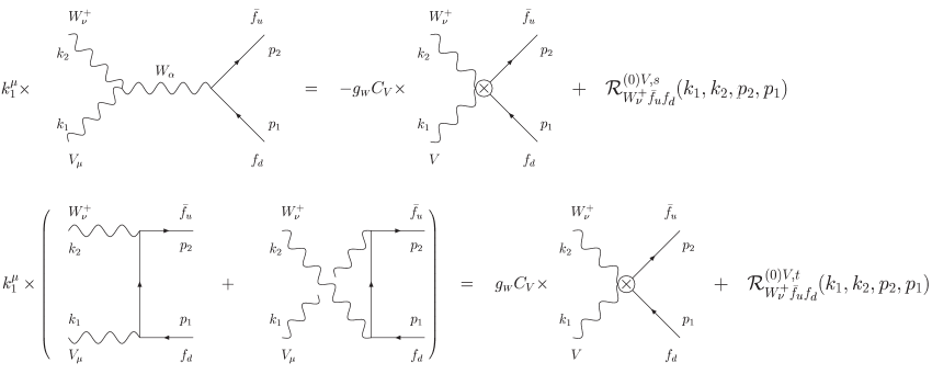
Notice that the above - decomposition is ambiguous in the presence of longitudinal momenta, since their action can change the topology of a given Feynman diagram. Let us consider in fact the action of a longitudinal momentum, say , on the amplitude . In this case, the WI of Eq.(3.10) will be triggered in the -channel graph, while that of Eq.(3.4) in the -channel one. In particular, isolating the “pinched” terms, one has (Fig.1)
| (4.10) |
Notice that the first term in the first equation above, even if it comes from a -channel graph, is in fact propagator-like. Adding by parts the two equations we enforce the PT - cancellation, thus getting the result
| (4.11) |
It is interesting to see how the very same cancellation applies also in the neutral gauge-boson sector. Consider in fact the tree-level amplitude : once again we can decompose the amplitude into its - and -channel parts, given by
| (4.12) |
where
| (4.13) |
When contracted by a longitudinal momentum we will then have the results (Fig.2)
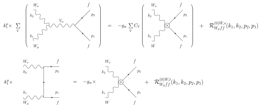
| (4.14) |
where we have defined the effective current as
| (4.15) |
which should not be confused with the usual current of Eq.(4.9). Adding by parts Eq.(4.14), we get finally
| (4.16) |
The first line of the right-hand side (rhs) of the above equation is always zero, independently on the external (on-shell) leptons, reflecting the well known property of process independence of the PT algorithm. If we choose down leptons, the zero is due to the identity
| (4.17) | |||||
In the case we choose right-handed polarized down leptons instead, while there is no term (there are no boxes in such case), the cancellation continue to be true due to the identity
| (4.18) |
Finally, if we consider up leptons there is no coupling with the photon in the channel, but still the cancellation goes through since one has that
| (4.19) |
(notice that in this case the contribution of the -channel graph has an extra minus sign due to a permutation of the gauge bosons in the trilinear vertex).
The reader can easily convince him-/her-self that the very same kind of - cancellation manifest itself in exactly the same way when considering the SM scalar sector (both in the charged as well as in the neutral case), by calculating the divergence of the corresponding amplitudes , , and .
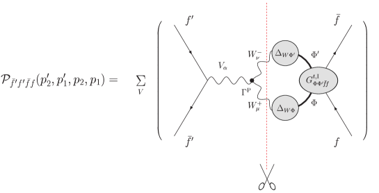
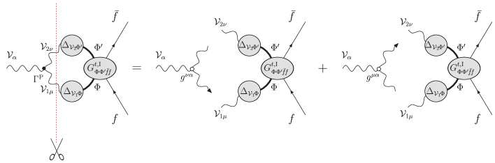
The (tree-level) - cancellations outlined above are in fact a consequence of the underlying BRST symmetry, and as such they will continue to occur at higher orders; thus the correct way to look at them is through the use of the STIs. To fix the ideas let us consider the neutral gauge-boson sector, and denote by the subset of graphs of our process that will receive the action of the longitudinal momenta stemming from the pinching part of the gauge-boson trilinear vertices . Since the decomposition is carried out only on the external vertices, we have that (see Fig.3)
| (4.20) | |||||
where we have defined the integral measure
| (4.21) |
with , the space-time dimension, and the ’t Hooft mass. Clearly, there is an equal contribution from the situated on the right hand-side of .
Let us focus on the (on-shell) STI satisfied by the amplitude ; the latter is listed in the appendix [Eq.(1.8)] and it is of the form
| (4.22) |
Now, as already discussed in our tree-level examples, in perturbation theory both and are given by Feynman diagrams, which can be separated into distinct classes, depending on their kinematic dependence and their geometrical properties. In addition to the aforementioned - decomposition, Feynman diagrams can be also separated into one-particle irreducible (1PI) and one-particle reducible (1PR) ones. In particular, 1PR graphs are those which, after cutting one line, get disconnected into two subgraphs none of which is a tree-level graph; if this does not happen, then the graph is 1PI. The crucial point is that the action of the momenta or on does not respect, in general, the original - and 1PI-1PR separation furnished by the Feynman diagrams (see third paper of [4]).
In other words, even though Eq.(4.22) holds for the entire amplitude, it is not true for the individual sub-amplitudes, i.e.,
| (4.23) |
where I (respectively R) indicates the one-particle irreducible (respectively reducible) parts of the amplitude involved. Evidently, whereas the characterization of graphs as propagator- and vertex-like is unambiguous in the absence of longitudinal momenta (e.g., in a scalar theory), their presence tends to mix propagator- and vertex-like graphs. Similarly, 1PR graphs are effectively converted into 1PI ones (the opposite cannot happen). The reason for the inequality of Eq.(4.23) are precisely the propagator-like terms, such as those encountered in our tree-level examples and in the one- and two-loop PT calculations [2]; they have the characteristic feature that, when depicted by means of Feynman diagrams contain unphysical vertices, i.e., vertices which do not exist in the original Lagrangian. All such diagrams cancel diagrammatically against each other. Thus, after the PT cancellations have been enforced, we find that the -channel irreducible part satisfies the identity
| (4.24) |
since, in this case, all the possible mixing due to the presence of the longitudinal momenta, has been taken into account.
Of course these observations apply also to the gauge-boson charged sector case as well as to the scalar sector. The non-trivial step for generalizing the PT to all orders is then the following: Instead of going through the arduous task of manipulating the left hand-side of Eq.(4.24) in order to determine the pinching parts and explicitly enforce their cancellation, use directly the right-hand side, which already contains the answer! Indeed, the right-hand side involves only conventional (ghost) Green’s functions, expressed in terms of normal Feynman rules, with no reference to unphysical vertices. This algorithm has been successfully implemented in the QCD case; in the next two sections we will see that it gives rise to the PT vertices with the expected properties to all orders.
5 The PT gauge-boson–fermion–fermion vertex
This section contains one of the central result of the present paper, namely the all-order PT construction of the gauge-boson–fermion–fermion vertex, with the gauge-boson off-shell and the fermions on-shell. By virtue of the observations made in the previous section, the derivation presented here turns out to be particularly compact.
Before entering into the detailed calculations, a note on the notation. To avoid notational clutter we will refrain, in what follows, to indicate redundant indices in the Green’s functions. Thus, we will remove from them all the references to the external fermions and their momenta, since the latter are irrelevant for the PT construction (which is independent of the external particle chosen). Thus, for example, the four point amplitudes and , will read and respectively.
5.1 Charged gauge-boson sector
We begin with the construction of the PT vertex ( from now on). To achieve this, we classify all the diagrams that contribute to this vertex in the FG, into the following types (Fig.4): (i) those containing an external (tree-level) three-gauge-boson vertex, i.e., those containing a three-gauge-boson vertex where the momentum is incoming, and (ii) those which do not have such an external vertex. This latter set contains graphs where the incoming gauge-boson couples to the rest of the diagram with any other type of interaction vertex other than a three-gauge-boson vertex. Thus we write
| (5.1) |
where, according to our definitions,
| (5.2) |
In Eq.(5.2) we have , , and , and the sum is over all the allowed permutations and combinations of fields.
As a second step, we next carry out the characteristic PT vertex decomposition of Eq.(3.7) to the external three-gauge-boson vertex appearing in the class (i) diagrams, i.e. we define
| (5.3) |
For the case at hands then
| (5.4) | |||||
where the integral measure has been defined in (4.21). Following the discussion presented in the previous section, the pinching action amounts then to using the STIs of Eqs.(1.2) and (1.6) for making the replacements (Fig.5)
| (5.5) | |||||
and similarly for the term involving the amplitude, or, equivalently,
| (5.6) | |||||
At this point the construction of the effective PT vertex has been completed, and we have
| (5.7) | |||||
We pause here to make a comment about the above result. What we want to stress is that Eq.(5.7) is provided as it is by blindly following the PT prescriptions given in the previous sections. On the other hand, one may now ask if there exists Feynman rules which can be employed has a shortcut to compute PT Green’s functions, such as the vertex function of Eq.(5.7). It turns out that at the one- and two-loop level the answer to this question is positive, and the needed Feynman rules are in fact provided by the BFM ones at the special value [background Feynman gauge (BFG for short)].
In what follows we will show that the effective PT vertex and the gauge-boson–fermion–fermion vertex written in the BFG are in fact equal. For doing this we first of all observe that part of the type (ii) diagrams contained in the original FG vertex, carry over to the same sub-groups of BFG graphs. In fact, in the BFM all of the vertices involving fermions have the usual form, so that we have
| (5.8) |
Moreover, since the BFM gauge-fixing term is quadratic in the quantum fields, apart from vertices involving ghost fields, only vertices containing exactly two quantum fields can differ from the conventional FG ones. Thus the vertices (respectively ) involving one background gauge-boson and three quantum gauge-boson (respectively one quantum gauge-boson and two quantum scalars) coincide with the FG vertices (respectively ), so that
| (5.9) |
Finally, as far as the vertices involving two quantum fields are concerned, we have that the vertex coincides with the corresponding FG vertex , and that the vertex coincides with the part of the PT decomposition Eq.(3.7). Thus we have the identities
| (5.10) |
The final step is to recognize that the BFG ghost and scalar–gauge-boson sectors will be provided precisely by combining the remaining FG class (ii) diagrams with the terms appearing on the right hand-side of Eq.(5.7). Specifically we will reproduce the symmetric vertex characteristic of the BFG, as well as the and the vertices (the last vertex being totally absent in the FG).
Now the form of the relevant terms appearing in Eq.(5.6), is given in Eqs.(1.5) and (1.7) of the Appendix. In particular the -channel irreducible part of these identities has precisely the same form provided that we replace the kernels appearing in the original STIs by the corresponding -channel irreducible kernels . Our analysis of the PT terms starts then from the terms which are of the type and that are absent in the FG formalism. Then, these terms read
| (5.11) |
where we have used the fact that . It is then straightforward to check that the above terms correspond precisely to the BFG sector of the theory, i.e., we have
| (5.12) |
The remaining PT terms mix instead with the corresponding class (ii) contributions. For the ghost sector we have in fact that the class (ii) diagrams amount to the contribution
| (5.13) | |||||
which, when added to the corresponding PT terms, gives
| (5.14) | |||||
i.e., we have recovered the symmetric BFG ghost sector,
| (5.15) |
Finally, the class (ii) contributions for the gauge-boson–scalar sector, reads
| (5.16) | |||||
where and . One should notice that there is no FG coupling: the corresponding BFG vertex must be entirely generated from the PT terms. Adding in fact the PT terms to the above contributions we get the result
| (5.17) | |||||
Now, the first two terms in the above expression corresponds precisely to the BFG vertex , while represents the BFG coupling. Therefore, we find that
| (5.18) |
This concludes the proof of the (all-order) identity (putting back the fermionic indices)
| (5.19) |
We emphasize that the sole ingredient used in the above construction has been the STIs of Eqs.(1.2) and (1.6); in particular at no point have we employed an a priori knowledge of the background field formalism. Instead both its special ghost sectors, as well as the different vertices involving two quantum fields has arisen dynamically, and, at the same time, projected out to the special value . As we will see this will be always the case.
5.2 Neutral gauge-boson sector
As in the charged case, we start by defining the class (i) diagrams as
| (5.20) |
In the neutral sector there is only one class (i) term, and, after carrying out the usual decomposition, we have
| (5.21) |
Using the STIs of Eq.(1.8), we have that the pinching action amounts to the replacement
| (5.22) |
which gives in turn the PT vertex
| (5.23) | |||||
We can now compare the PT result with the BFG one. For the same reasons discussed in the charged case, we have the following identities
| (5.24) |
On the other hand once again the BFG ghost sector and gauge-boson–scalar sector will be dynamically generated through PT terms or the combination of PT terms and class (ii) diagrams. The relevant terms appearing in Eq.(5.23) are shown in Eq.(1.9); in particular we find that, as in the previous case, the PT terms of the type are responsible for the dynamical generation of the corresponding BFG sector, i.e., we have
| (5.25) |
where
| (5.26) |
The remaining PT contributions mixes with the corresponding class (ii) diagrams, therefore generating the BFG modified sector of the theory. In fact, the class (ii) diagrams contribution to the ghost sector reads
| (5.27) | |||||
so that by adding them to the PT terms, we get
| (5.28) |
which represents the BFG symmetric ghost sector, i.e.
| (5.29) |
Finally, the class (ii) diagrams contributing to the gauge-boson–scalar sector, can be written as
| (5.30) | |||||
Notice that in the BFG there is no coupling between the background photon and the fields, so that the above terms should precisely cancel (for ) the PT contributions. In fact, adding the two terms we find
| (5.31) |
where turns out to be the BFG coupling, i.e. and . Thus we have the identity
| (5.32) |
which finally show that, also for the neutral gauge boson sector, the PT result coincides with the BFG ones, i.e., putting back the fermion indices,
| (5.33) |
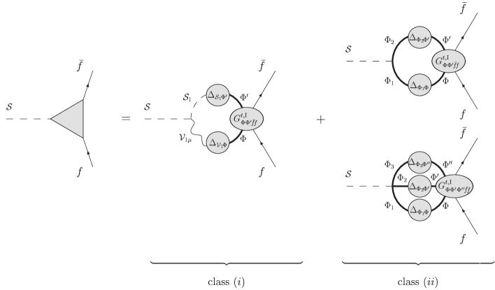
6 The PT scalar–fermion–fermion vertex
As explained in the earlier, when dealing with spontaneously broken theories, longitudinal momenta appear also in the vertices involving two scalar fields and one gauge-boson field, and thus must be included in the PT procedure. In the next two subsections we discuss the PT reorganization of the charged and neutral scalar sectors in details, proving once again the correspondence between the PT effective vertices and the BFG ones.
6.1 Charged scalar sector
The procedure to be applied in the scalar sector is very similar to the one used in the gauge-boson sector. One starts by classifying all the diagrams that contribute to this vertex in the FG, into the following types (Fig.6): (i) those containing an external (tree-level) scalar–scalar–gauge-boson vertex, i.e., those containing a scalar–scalar–gauge-boson vertex where the momentum is incoming, and (ii) those which do not have such an external vertex. This latter set contains graphs where the incoming gauge-boson couples to the rest of the diagram with any other type of interaction vertex other than a scalar–scalar–gauge-boson vertex. Thus, in the charged scalar case, we write
| (6.1) |
where, according to our definitions,
As a second step, we next carry out the characteristic PT vertex decomposition of Eq.(3.12) to the external scalar–scalar–gauge-boson vertex appearing in the class (i) diagrams, i.e. we define
| (6.3) |
In the case at hands then
| (6.4) |
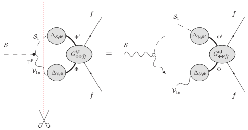
where the index runs over the neutral fields only, i.e. , with and . The pinching action amounts then to using the STIs of Eq.(1.10) for making the replacement (Fig.7)
| (6.5) |
so that the effective PT vertex will be given by
We then can proceed to the comparison with the corresponding BFG vertex . We start by observing that the vertices , and coincide with the corresponding FG vertices , and ; moreover, the vertices coincide with the part of the corresponding PT decomposition of Eq.(3.12). Thus we have the following identities
| (6.7) |
Let us once again turn our attention on the PT terms given in Eqs.(1.11) and (1.12), and start our analysis from the four particle sector of the type. Now, as far as the corresponding BFG sector is concerned, one should notice that there is no BFG coupling such as : in fact, there is a perfect cancellation between the PT terms involving the kernel appearing in and ( and respectively), while the terms involving the kernel carry a half of the corresponding BFG coupling and add up. It is then straightforward to check that the PT terms
| (6.8) | |||||
give rise to the correct BFG four particle ghost sector, i.e., that
| (6.9) |
For getting the remaining BFG sectors of the theory, one has also to consider the corresponding class (ii) diagrams. The FG contributions to the ghost sector reads in fact
| (6.10) | |||||
Now we notice that on the one hand there is no FG coupling, so that the BFG will be generated entirely from the PT terms; on the other hand the PT terms do not involve the kernel , which tell us that the FG coupling and the BFG one should coincide (as indeed happens to be true). Thus adding the two contributions we get
| (6.11) |
where is such that and . But the latter couplings are precisely the corresponding BFG ones so that we have the identity
| (6.12) |
The last sector one needs to check is the scalar–scalar one. To this end we start by noticing that the FG contributions to this sector will contain only (external) Higgs fields, and read
| (6.13) | |||||
The BFG coupling will be thus completely generated from the PT terms, combining the terms proportional to the (external) field kernel appearing in , and . Adding all the terms we find in fact
| (6.14) |
where represents the corresponding BFG coupling, i.e., and . We thus have that
| (6.15) |
which represents the last identity we need for proving that (putting back the fermionic indices)
| (6.16) |
6.2 Neutral scalar sector
In the neutral scalar sector case, the class (i) diagrams allow for the following PT decomposition
| (6.17) |
with
| (6.18) |
In the above expressions we have that is (respectively, ) when (respectively, ), and that (respectively, ) when (respectively, ).
Through the use of the STIs of Eq.(1.13), the pinching action amount in this case to the following replacement
| (6.19) | |||||
so that the effective PT vertex will be given by
| (6.20) | |||||
We can now proceed to the comparison with the corresponding BFG vertex. We first of all notice that as in the charged scalar case we have the following identities
| (6.21) |
Next, we concentrate on the PT terms [shown in Eqs.(1.14) and (1.15)], starting from the four particle sector of the type. It is then a long but straightforward exercise to check that the PT terms
| (6.22) |
generate the four particles BFG ghost sector, i.e.,
| (6.23) |
The remaining PT terms will mix with the corresponding class (ii) diagrams. In particular, as far as the remaining part of the ghost sector is concerned, the FG contributions reads
| (6.24) | |||||
At this point we observe that the background field does not couple with (two) ghosts, so that the PT terms must precisely cancel the FG ones. In fact, after adding the two contributions, one can easily check that
| (6.25) |
correctly reproduces the BFG sector, i.e.,
| (6.26) |
We finally need to consider the scalar–scalar sector. The FG contributions to the latter read
| (6.27) | |||||
Now, we first of all notice that the BFG vertex and the BFG one coincide; moreover since there is no BFG coupling, the PT terms should exactly vanish in this case, since there is no FG coupling either. After adding the PT contributions to the above terms, one has the result
| (6.28) |
which precisely coincide with the BFG one, i.e we have
| (6.29) |
This concludes the proof that (putting back fermionic indices)
| (6.30) |
7 Reconstruction of the PT terms: two-point functions
Of course at this point one would expect that the two-point functions too coincide with the BFG ones, since both the boxes as well as the vertices coincide with the corresponding quantities in the BFG, and the -matrix is unique. A proof based on the strong induction principle along the same lines of the one carried out in [22] for the QCD case can be easily carried out.
In this section however, we are going to briefly address a slightly different question that is: can one explicitly reconstruct the pinching parts that implicitly cancel in our all-order generalization of the PT procedure? or, equivalently, can one explicitly construct the two-point PT functions? The use of the BQIs of Eq.(2.1) and (LABEL:AVBQI) will allow a positive answer to both questions.
To fix the ideas we will hereafter consider the charged electroweak sector, i.e., we choose and , so that the BQIs of Eq.(LABEL:AVBQI) read
| (7.1) |
where we have omitted the momentum dependence of the various Green’s function as for the rest of this section [the latter can be easily reconstructed from the appendix equations (2.1) and (LABEL:AVBQI)].
On the other hand, due to our explicit construction, we know that in general and , so that the above BQIs express (to all orders) the relations between the PT three point Green’s functions and the normal ones, and (upon inversion) viceversa.
To extract the propagator-like pieces from the above BQIs, one has to isolate all the terms proportional to the tree-level vertices and . The complete set of these terms can be found inverting at each perturbative order Eqs.(7.1) thus writing the three points Green’s functions in terms of the PT ones, and observing that at tree-level they coincide. It is clear from the structure of Eq.(7.1) that the propagator-like pieces extracted from the BQI (respectively, ) will contain in general both the two points functions and (respectively, and ).
After isolating the propagator-like terms one has to decide how to allot them among the available two point functions , , and . At a first sight, it is tempting to assign the () part entirely to the () self-energy, while giving the term proportional to () to the mixed function (). To see that this is however not the case, we notice that at one-loop (respectively, ), but still the BQIs should provide contribution for both the as well as the two-point functions (respectively, and ).
The correct procedure is instead the following [36]:
-
i)
To isolate from the terms proportional to the corresponding two type of contributions, we insert the identity
(7.2) When looking at the BQI for (respectively, ) the first term will contribute to the (respectively, ) PT two point function, while the second to the (respectively, ) one.
-
ii)
To isolate from the terms proportional to the corresponding two type of contributions, we instead make use of the following relation, holding when contracted with on-shell spinors
(7.3) When looking at the BQI for (respectively, ) the first term will contribute to the (respectively, ) PT two point function, while the second to the (respectively, ) one.
At the one-loop level one has for example that
| (7.4) |
Making use of Eqs.(7.2) and (7.3) we then find
| (7.5) | |||||
Therefore, taking into account the mirror vertices, we end up with the results
| (7.6) |
Inspection of the above expressions shows that they coincide precisely with the one-loop expansion of the BQIs of Eq.(2.1), thus we recover the well known results
| (7.7) |
More involved is the analysis in the two-loop case, where the BQIs for the vertex functions read
| (7.8) | |||||
To extract the corresponding propagator-like pieces we can make use, as in the previous case, of the identities of Eq.(7.2) and (7.3). However beyond the one-loop level this is not the end of the story: the conversion of the 1PR string of (normal) one-loop self-energies into the corresponding string of one-loop PT self-energies has to be taken into account. This will generated the 1PI contributions that have to be allotted to the corresponding two-loop PT two-point functions.
Therefore, after adding the mirror vertex contributions, we have the results
| (7.9) |
Moreover, following the second paper of [4] we find,
| (7.10) |
8 Conclusions
In the present paper we have extended the algorithm presented in [22] for generalizing the PT to all orders in QCD, to the case of the electroweak sector of the SM. This generalization has been a pending problem, mainly due both to the proliferation of Feynman diagrams as compared to the QCD case, as well as to the complication arising from the presence of Goldtone’s bosons in the theory, which implies that the BRST symmetry (and therefore the STIs) are now realized through them. These problems have been solved by resorting to the recently introduced PT construction by means of the STI satisfied by special four-point functions which serve as a common kernel to all higher order self-energy and vertex diagrams. Thus, instead of manipulating algebraically individual Feynman diagrams, all the pinching action could be simultaneously addressed. In particular, we have shown that without any modification (apart from the obvious one of the inclusion of the vertices of the type as sources of pinching momenta in the scalar sector), the QCD algorithm goes through in the SM case, allowing for the all-order generalization of the PT.
It should be clear by now that, being valid to all orders, the PT is a procedure intrinsic to any gauge theory (Abelian and non-Abelian), that can be applied to obtain Green’s functions possessing many of the properties of -matrix elements. This is particularly important in the SM case, in which the consistent description of unstable particles necessitates the definition and resummation of off-shell (two-point) Green’s functions, which must respect the crucial physical requirements of resummability, analiticity, unitarity, gauge invariance, multiplicative renormalization and no shifting of the position of the pole [4]. This is naturally provided by the PT two-point functions to all orders.
The correspondence between the PT Green’s functions and the BFG ones, that we have shown to persist to all order, has been a source of considerable confusion in the literature; in particular it has been argued that the PT is but a special case of the BFM, representing one out of an infinite number of equivalent choices parametrized by the gauge fixing parameter. One should however recall that for a general value of the latter parameter, the BFM Green’s functions shows a residual dependence on it. Thus, from the PT point of view there is no difference between a theory quantized in the BFM or gauges: in fact, to eliminate this residual dependence of the BFM Green’s functions, one would apply the very same PT algorithm discussed in this paper (but with the STIs written down in this gauge), and arrive at precisely the same vertices and propagators we have described. The BFG has only the special property that pinching contribution vanishes, and thus is the most economical way of obtainig the PT results. In addition, the PT construction goes through unaltered, under circumstances where the BFM Feynman rules cannot even be applied. Specifically, if instead of an -matrix element one were to consider a different observable, such as a current-current correlation function or a Wilson loop, as was in fact done by Cornwall in the original formulation [1] (and, more recently, in [17]), one could not start out using the BFM Feynman rules, because all fields appearing inside the first non-trivial loop are quantum ones. Instead, by following the PT rearrangement inside these physical amplitudes one would dynamically arrive at the BFM answer.
Notice that the renormalization program will not spoil the PT construction presented here. Of course there is no doubt that if one supplies the correct set of counterterms within the conventional formulation the entire -matrix will continue to be renormalized, even after the PT rearrangements of the (unrenormalized) Feynman graphs. The question is eventually if the new Green’s functions constructed through the PT rearrangements are individually renormalizable (a classic counter example being the unitary gauge of the SM, where the entire -matrix is renormalizable, whereas the individual Green’s functions computed in this gauge are not). The general methodology for dealing with this issue has been established in the second paper of [2], where the two-loop QCD case was studied in detail, and consist of two steps: one should first of all start out with the counterterms which are necessary to renormalize individually the conventional Green’s functions contributing to the -loop -matrix in the RFG; then, one should show that, by simply rearranging these counterterms, following the PT rules, we arrive at the renormalized -loop PT Green’s functions. This analysis was extended to the (QCD) all order case in the second paper of [22], where it was shown that renormalization poses no problems whatsoever to the PT construction. The generalization of the above analysis to the SM case does not present any additional conceptual complication.
The extension of the PT to theories beyond the SM should pose (at least at the one-loop level) no problems at all, and has been recently pursued in the MSSM [19], in the context of finding a scale and gauge independent definition of mixing angles for scalar particles. It remains to be seen what Feynman rules give rise to these super-PT Green’s functions in theories possessing many scalars in the spectrum (such as the MSSM), since in the latter case (contrary to the SM one) one has, in principle, the freedom to include (or not) in the BFM gauge fixing function also scalars that do not posses a vev (such as squarks), therefore symmetrizing (or not) the corresponding coupling. To the best of our knowledge, it is not yet clear which one (if any) of the above possible choices will constitute the super-BFM gauge of the MSSM. However notice that the PT procedure has no arbitrariness whatsoever (contrary to the claims in [19]), and moreover naturally select a super-BFM gauge fixing function where all the scalars have been put, since we have seen that one should pinch whenever a longitudinal momenta appears in the external tree-level vertex of type (i) diagrams (and this will happen for all the vertices of the type , irrespectively from whether or not the scalar has a vev). We conjecture that the MSSM super-BFM gauge will coincide with the one dynamically projected out by the super-PT procedure.
Clearly, it would also be very interesting to reach a deeper understanding of why the PT dynamically singles out the BFG value . There are several pieces of evidence that the BFG is somehow special; for example, the anomalous one-loop SUSY breaking in Yang-Mills theories with local coupling is uniquely determined by the BFG value of a certain vertex function [37]. One possible direction to explore would be to look for special properties of the BFM action at ; an interesting 3D example of a field-theory, which, when formulated in the background Landau gauge (), displays an additional (non-BRST related) rigid super-symmetry, is given in [38].
Concluding, we think that many of the open questions related to the PT procedure, such as its uniqueness, independence from the test particles and especially its generalization beyond leading order, have been fully addressed and solved, both in theories with, as well as without, spontaneous symmetry breaking. Moreover, a deep connection between the PT and powerful BRST related algebraic formalisms (such as the ones of Batalin-Vilkovisky and Nielsen) has been unveiled, allowing the PT to acquire the status of a well-defined formal tool.
All the figures of this paper have been drawn with JaxoDraw [39]. Visit the JaxoDraw home page
http://altair.ific.uv.es/~JaxoDraw/home.html to know more about it.
Appendix A Slavnov-Taylor identities
In this appendix we briefly discuss the derivation of the (on-shell) STIs needed, by taking as a case study the STI satisfied by the amplitude when hitting from the neutral gauge boson side.
For getting this STI one starts by observing that the BRST transformation of an antighost-field starts with the term (which is in momentum space). In this particular case we then trade the gauge boson field for the anti-ghost field , and consider the trivial (due to ghost charge conservation) identity
| (1.1) |
leaving the fermionic fields unspecified. By applying the BRST operator to the above identity, and passing to momentum space, we get the identity
| (1.2) | |||||
where (FT stands for Fourier transform)
| (1.3) |
and two fields between brackets are taken to be at the same space-time position. A diagrammatic representation of the Green’s functions appearing above is shown in Fig.(8).
Now let us concentrate on the terms. From the BRST variations of Eq.(2.22), it is clear that independently of the type of fermions appearing in Eq.(1.3), these terms will miss an external fermion propagator, and will thus vanish due to the on-shell condition. At one-loop order, for example, these terms represent simply the ones proportional to the inverse tree-level propagator appearing in the PT calculations. Indeed, we can multiply both sides of the Eq.(1.2) by the product of the two inverse propagator of the external fermions, and then sandwich the amplitude between their spinors: due to the on-shell conditions the vanishing of the aforementioned terms follows by virtue of the Dirac equation. One should observe that the vanishing of these on-shell pieces is in fact the reason for the (all order) process independence of the PT algorithm [40, 22].
Thus one arrives at the following (on-shell) STI
| (1.4) |
where, omitting the spinors,
| (1.5) | |||||
In Eq.(1.5) (as in the rest of these Appendices), a sum over twice repeated fields (running over all the allowed SM combinations) is intended.
In what follows we list all the remaining on-shell STIs used throughout the paper.
A.1 Gauge-boson sector
A.1.1 Charged sector
A.1.2 Neutral sector
In this case the STIs needed are just
| (1.8) |
where we have
| (1.9) | |||||
A.2 Scalar bosons sector
A.2.1 Charged sector
The STIs employed in this case reads
| (1.10) |
where runs over the neutral would-be Goldstone bosons only, i.e., . In particular we have
| (1.11) | |||||
with and , and
| (1.12) | |||||
where is (respectively, ) when (respectively, ), and (respectively, ) when (respectively, ).
A.2.2 Neutral sector
Finally, in the neutral scalar sector the following STIs appear
| (1.13) |
where we have
| (1.14) | |||||
and
| (1.15) | |||||
Appendix B Background quantum identities
In this appendix we report the BQIs used in the paper. Details on how to derive them can be found in [29, 30].
B.1 Two-point functions
The BQIs for the two-point functions read
| (2.1) | |||||
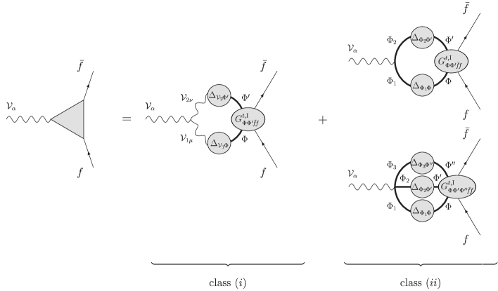
B.2 Three-point functions
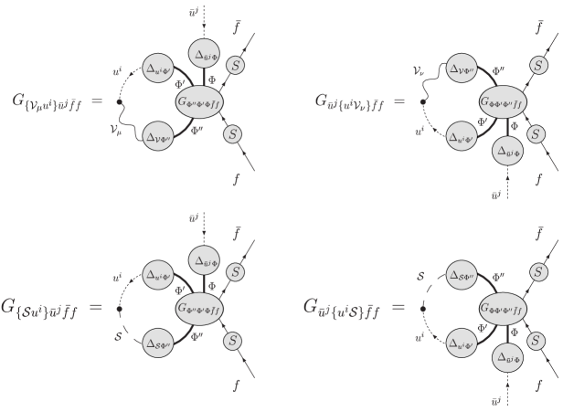
Neglecting pieces that vanish when considering the external fermions to be on-shell, the BQIs for the three-point functions read
Notice that the Green’s functions that provide the reorganization of the Feynman diagrams for converting the three-point background functions into the corresponding quantum ones are precisely the same that appear in the two-point functions of Eq.(2.1).
References
References
- [1] J. M. Cornwall, Phys. Rev. D26 (1982) 1453; J. M. Cornwall, J. Papavassiliou, Phys. Rev. D40 (1989) 3474; J. Papavassiliou, Phys. Rev. D41 (1990) 3179; G. Degrassi and A. Sirlin, Phys. Rev. D46 (1992) 3104.
- [2] J. Papavassiliou, Phys. Rev. Lett. 84 (2000) 2782; Phys. Rev. D62 (2000) 045006.
- [3] M. J. Veltman, Physica 29 (1963) 186; W. W. Repko and C. J. Suchyta, Phys. Rev. Lett. 62 (1989) 859; S. Dawson and S. Willenbrock, Phys. Rev. D40 (1989) 2880; A. Pilaftsis, Z. Phys. C47 (1990) 95; A. Dobado, Phys. Lett. B237 (1990) 457; A. Sirlin, Phys. Rev. Lett. 67 (1991) 2127; A. Sirlin, Phys. Lett. B267 (1991) 240; R. G. Stuart, Phys. Lett. B262 (1991) 113; R. G. Stuart, Phys. Lett. B272 (1991) 353; R. G. Stuart, Phys. Rev. Lett. 70 (1993) 3193; M. Nowakowski and A. Pilaftsis, Z. Phys. C60 (1993) 121; A. Aeppli, G. J. van Oldenborgh and D. Wyler, Nucl. Phys. B428 (1994) 126; U. Baur and D. Zeppenfeld, Phys. Rev. Lett. 75 (1995) 1002; M. Beuthe, R. Gonzalez Felipe, G. Lopez Castro and J. Pestieau, Nucl. Phys. B498 (1997) 55; D. Wackeroth and W. Hollik, Phys. Rev. D55 (1997) 6788; M. Passera and A. Sirlin, Phys. Rev. D58 (1998) 113010; B. A. Kniehl and A. Sirlin, Phys. Rev. Lett. 81 (1998) 1373.
- [4] J. Papavassiliou, A. Pilaftsis, Phys. Rev. Lett. 75 (1995) 3060; Phys. Rev. D53 (1996) 2128; Phys. Rev. D54 (1996) 5315; Phys. Rev. Lett. 80 (1998) 2785; Phys. Rev. D58 (1998) 053002.
- [5] J. M. Cornwall, D. N. Levin and G. Tiktopoulos, Phys. Rev. D10 (1974) 1145; C. E. Vayonakis, Lett. Nuovo Cim. 17 (1976) 383; M. S. Chanowitz and M. K. Gaillard, Nucl. Phys. B261 (1985) 379; G. J. Gounaris, R. Kogerler and H. Neufeld, Phys. Rev. D34 (1986) 3257.
- [6] K. Fujikawa, B. W. Lee, A. I. Sanda, Phys. Rev. D6 (1972) 2923.
- [7] J. Papavassiliou, K. Philippides, Phys. Rev. D48 (1993) 4255.
- [8] J. Papavassiliou, C. Parrinello, Phys. Rev. D50 (1994) 3059.
- [9] J. Bernabeu, L. G. Cabral-Rosetti, J. Papavassiliou, J. Vidal, Phys. Rev. D62 (2000) 113012.
- [10] J. Bernabeu, J. Papavassiliou, J. Vidal, Phys. Rev. Lett. 89 (2002) 101802; arXiv:hep-ph/0210055, Nucl. Phys. B to appear; J. Papavassiliou, J. Bernabeu, D. Binosi and J. Vidal, arXiv:hep-ph/0310028.
- [11] G. Degrassi, B. A. Kniehl, A. Sirlin, Phys. Rev. D48 (1993) 3963.
- [12] J. Papavassiliou, K. Philippides, K. Sasaki, Phys. Rev. D53 (1996) 3942.
- [13] S. Nadkarni, Phys. Rev. Lett. 61 (1988) 396; G. Alexanian, V. P. Nair, Phys. Lett. B352 (1995) 435; M. Passera, K. Sasaki, Phys. Rev. D54 (1996) 5763; K. Sasaki, Phys. Lett. B369 (1996) 117.
- [14] J. Papavassiliou, E. de Rafael, N. J. Watson, Nucl. Phys. B503 (1997) 79. D. Binosi, J. Papavassiliou, Nucl. Phys. Proc. Suppl. 121 (2003) 281.
- [15] K. Hagiwara, S. Matsumoto, D. Haidt, C. S. Kim, Z. Phys. C64 (1994) 559.
- [16] A. Pilaftsis, Nucl. Phys. B504 (1997) 61.
- [17] D. Binosi, J. Papavassiliou, Phys. Rev. D65 (2002) 085003.
- [18] Y. Yamada, Phys. Rev. D64 (2001) 036008; A. Pilaftsis, Phys. Rev. D65 (2002) 115013.
- [19] J. R. Espinosa, Y. Yamada, Phys. Rev. D67 (2003) 036003.
- [20] A. Ferroglia, G. Ossola, A. Silin, arXiv:hep-ph/0307200.
- [21] M. Binger, S. J. Brodsky, arXiv:hep-ph/0310322.
- [22] D. Binosi, J. Papavassiliou, Phys. Rev. D66 (2002) 111901; J. Phys. G30 (2004) 203; arXiv:hep-ph/0310149.
- [23] B. S. Dewitt, Phys. Rev. 162 (1967) 1195; J. Honerkamp, Nucl. Phys. B48 (1972) 269; R. E. Kallosh, Nucl. Phys. B78 (1974) 293; H. Kluberg-Stern, J. B. Zuber, Phys. Rev. D12 (1975) 482; I. Y. Arefeva, L. D. Faddeev, A. A. Slavnov, Theor. Math. Phys. 21 (1975) 1165; G. ’t Hooft, in: *Karpacz 1975, Proceedings, Acta Universitatis Wratislaviensis*, Vol. 1, No. 368, Wroclaw, 1976, pp. 354; S. Weinberg, Phys. Lett. B91 (1980) 51; L. F. Abbott, Nucl. Phys. B185 (1981) 189; G. M. Shore, Ann. Phys. 137 (1981) 262; L. F. Abbott, M. T. Grisaru, R. K. Schaefer, Nucl. Phys. B229 (1983) 372; C. F. Hart, Phys. Rev. D28 (1983) 1993; A. Rebhan, G. Wirthumer, Z. Phys. C28 (1985) 269.
- [24] S. Weinberg, The Quantum Theory of Fields, Vol. II, Cambridge University Press, New York, 1996.
- [25] A. Denner, G. Weiglein, S. Dittmaier, Phys. Lett. B333 (1994) 420; S. Hashimoto, J. Kodaira, Y. Yasui, K. Sasaki, Phys. Rev. D50 (1994) 7066.
- [26] D. Binosi, J. Papavassiliou, Phys. Rev. D66 (2002) 076010.
- [27] A. Denner, G. Weiglein, S. Dittmaier, Nucl. Phys. B440 (1995) 95.
- [28] I. A. Batalin, G. A. Vilkovisky, Phys. Lett. B69 (1977) 309; Phys. Rev. D28 (1983) 2567.
- [29] P. A. Grassi, T. Hurth, M. Steinhauser, Annals Phys. 288 (2001) 197; Nucl. Phys. B610 (2001) 215.
- [30] D. Binosi, J. Papavassiliou, Phys. Rev. D66 (2002) 025024.
- [31] G. Barnich, F. Brandt, M. Henneaux, Phys. Rept. 338 (2000) 439.
- [32] P. Gambino, P. A. Grassi, Phys. Rev. D62 (2000) 076002.
- [33] N. K. Nielsen, Nucl. Phys. B101 (1975) 173.
- [34] J. M. Cornwall and G. Tiktopoulos, Phys. Rev. D15 (1997) 2937.
- [35] B. J. Haeri, Phys. Rev. D38 (1988) 3799; A. Pilaftsis, Nucl. Phys. B487 (1997) 467.
- [36] J. Papavassiliou, Phys. Rev. D50 (1994) 5958.
- [37] E. Kraus, Phys. Rev. D65 (2002) 105003.
- [38] D. Birmingham, M. Rakowski, G. Thompson, Nucl. Phys. B329 (1990) 83.
- [39] D. Binosi and L. Theussl, arXiv:hep-ph/0309015.
- [40] N. J. Watson, Phys. Lett. B349 (1995) 155.