Instantons and the Spin of the Nucleon

Abstract

Motivated by measurements of the flavor singlet axial coupling constant of the nucleon in polarized deep inelastic scattering we study the contribution of instantons to OZI violation in the axial-vector channel. We consider, in particular, the $f_{1}-a_{1}$ meson splitting, the flavor singlet and triplet axial coupling of a constituent quark, and the axial coupling constant of the nucleon. We show that instantons provide a short distance contribution to OZI violating correlation functions which is repulsive in the $f_{1}$ meson channel and adds to the flavor singlet three-point function of a constituent quark. We also show that the sign of this contribution is determined by positivity arguments. We compute long distance contributions using numerical simulations of the instanton liquid. We find that the iso-vector axial coupling constant of a constituent quark is $(g_{A}^{3})_{Q}=0.9$ and that of a nucleon is $g_{A}^{3}=1.28$, in good agreement with experiment. The flavor singlet coupling of a quark is close to one, while that of a nucleon is suppressed, $g_{A}^{0}=0.77$. However, this number is larger than the experimental value $g_{A}^{0}=(0.28-0.41)$.

I Introduction

The current interest in the spin structure of the nucleon dates from the 1987 discovery by the European Muon Collaboration that only about 30% of the spin of the proton is carried by the spin of the quarks Ashman:1987hv . This results is surprising from the point of view of the naive quark model, and it implies a large amount of OZI (Okubo-Zweig-Iizuka rule) violation in the flavor singlet axial vector channel. The axial vector couplings of the nucleon are related to polarized quark densities by

$$g_{A}^{3} = \Delta u-\Delta d,$$ (1)

$$g_{A}^{8} = \Delta u+\Delta d-2\Delta s,$$ (2)

$$g_{A}^{0} \equiv \Delta\Sigma=\Delta u+\Delta d+\Delta s.$$ (3)

The first linear combination is the well known axial vector coupling measured in neutron beta decay, $g_{A}^{3}=1.267\pm 0.004$. The hyperon decay constant is less well determined. A conservative estimate is $g_{A}^{8}=0.57\pm 0.06$. Polarized deep inelastic scattering is sensitive to another linear combination of the polarized quark densities and provides a measurement of the flavor singlet axial coupling constant $g_{A}^{0}$. Typical results are in the range $g_{A}^{0}=(0.28-0.41)$, see Filippone:2001ux for a recent review.

Since $g_{A}^{0}$ is related to the nucleon matrix element of the flavor singlet axial vector current many authors have speculated that the small value of $g_{A}^{0}$ is in some way connected to the axial anomaly, see Dorokhov:ym ; Bass:1993bs ; Bass:2003vp for reviews. The axial anomaly relation

$$\partial^{\mu}A_{\mu}^{0}=\frac{N_{f}g^{2}}{16\pi^{2}}G_{\mu\nu}^{a}\tilde{G}_{\mu\nu}^{a}+\sum_{f}2m_{f}\bar{q}_{f}i\gamma_{5}q_{f}$$ (4)

implies that matrix elements of the flavor singlet axial current $A_{\mu}^{0}$ are related to matrix elements of the topological charge density. The anomaly also implies that there is a mechanism for transferring polarization from quarks to gluons. In perturbation theory the nature of the anomalous contribution to the polarized quark distribution depends on the renormalization scheme. The first moment of the polarized quark density in the modified minimal subtraction $(\overline{MS})$ scheme is related to the first moment in the Adler-Bardeen $(AB)$ scheme by Altarelli:1988nr

$$\Delta\Sigma_{\overline{MS}}=\Delta\Sigma_{AB}-N_{f}\frac{\alpha_{s}(Q^{2})}{2\pi}\Delta G(Q^{2}),$$ (5)

where $\Delta G$ is the polarized gluon density. Several authors have suggested that $\Delta\Sigma_{AB}$ is more naturally associated with the “constituent” quark spin contribution to the nucleon spin, and that the smallness of $\Delta\Sigma_{\overline{MS}}$ is due to a cancellation between $\Delta\Sigma_{AB}$ and $\Delta G$. The disadvantage of this scheme is that $\Delta\Sigma_{AB}$ is not associated with a gauge invariant local operator Jaffe:1989jz .

Non-perturbatively the anomaly implies that $g_{A}^{0}=\Delta\Sigma$ can be extracted from nucleon matrix elements of the topological charge density $g^{2}G^{a}_{\mu\nu}\tilde{G}^{a}_{\mu\nu}/(32\pi^{2})$ and the pseudoscalar density $m\bar{\psi}i\gamma_{5}\psi$. The nucleon matrix element of the topological charge density is not known, but the matrix element of the scalar density $g^{2}G^{a}_{\mu\nu}G^{a}_{\mu\nu}$ is fixed by the trace anomaly. We have Shifman:zn

$$\langle N(p)|\frac{g^{2}}{32\pi^{2}}G^{a}_{\mu\nu}G^{a}_{\mu\nu}|N(p^{\prime})\rangle=C_{S}(q^{2})m_{N}\bar{u}(p)u(p^{\prime}),$$ (6)

with $C_{S}(0)=-1/b$ where $b=11-2N_{f}/3$ is the first coefficient of the QCD beta function. Here, $u(p)$ is a free nucleon spinor. Anselm suggested that in an instanton model of the QCD vacuum the gauge field is approximately self-dual, $G^{2}=\pm G\tilde{G}$, and the nucleon coupling constants of the scalar and pseudoscalar gluon density are expected to be equal, $C_{S}(0)\simeq C_{P}(0)$ Anselm:1992wz , see also Kuhn:1990df . Using $g_{A}^{0}=N_{f}C_{P}(0)$ in the chiral limit we get $g_{A}^{0}\simeq-N_{f}/b\simeq-0.2$, which is indeed quite small.

A different suggestion was made by Narison, Shore, and Veneziano Narison:hv . Narison et al. argued that the smallness of $\Delta\Sigma=g_{A}^{0}$ is not related to the structure of the nucleon, but a consequence of the $U(1)_{A}$ anomaly and the structure of the QCD vacuum. Using certain assumptions about the nucleon-axial-vector current three-point function they derive a relation between the singlet and octet matrix elements,

$$g_{A}^{0}=g_{A}^{8}\frac{\sqrt{6}}{f_{\pi}}\sqrt{\chi^{\prime}_{top}(0)}.$$ (7)

Here, $f_{\pi}=93$ MeV is the pion decay constant and $\chi^{\prime}_{top}(0)$ is the slope of the topological charge correlator

$$\chi_{top}(q^{2})=\int d^{4}x\,e^{iqx}\,\langle Q_{top}(0)Q_{top}(x)\rangle,$$ (8)

with $Q_{top}(x)=g^{2}G^{a}_{\mu\nu}\tilde{G}^{a}_{\mu\nu}/(32\pi^{2})$. In QCD with massless fermions topological charge is screened and $\chi_{top}(0)=0$. The slope of the topological charge correlator is proportional to the screening length. In QCD we expect the inverse screening length to be related to the $\eta^{\prime}$ mass. Since the $\eta^{\prime}$ is heavy, the screening length is short and $\chi^{\prime}_{top}(0)$ is small. Equation (7) relates the suppression of the flavor singlet axial charge to the large $\eta^{\prime}$ mass in QCD.

Both of these suggestions are very interesting, but the status of the underlying assumptions is somewhat unclear. In this paper we would like to address the role of the anomaly in the nucleon spin problem, and the more general question of OZI violation in the flavor singlet axial-vector channel, by computing the axial charge of the nucleon and the axial-vector two-point function in the instanton model. There are several reasons why instantons are important in the spin problem. First of all, instantons provide an explicit, weak coupling, realization of the anomaly relation equ. (4) and the phenomenon of topological charge screening Schafer:1996wv ; Shuryak:1994rr . Second, instantons provide a successful phenomenology of OZI violation in QCD Schafer:2000hn . Instantons explain, in particular, why violations of the OZI rule in scalar meson channels are so much bigger than OZI violation in vector meson channels. And finally, the instanton liquid model gives a very successful description of baryon correlation functions and the mass of the nucleon Schafer:1993ra ; Diakonov:2002fq .

This paper is organized as follows. In Sect. II we review the calculation of the anomalous contribution to the axial-vector current in the field of an instanton. In Sect. III and IV we use this result in order to study OZI violation in the axial-vector correlation function and the axial coupling of a constituent quark. Our strategy is to compute the short distance behavior of the correlation functions in the single instanton approximation and to determine the large distance behavior using numerical simulations. In Sect. V we present numerical calculations of the axial couplings of the nucleon and in Sect. VI we discuss our conclusions. Some results regarding the spectral representation of nucleon three-point functions are collected in an appendix.

II Axial Charge Violation in the Field of an Instanton

We would like to start by showing explicitly how the axial anomaly is realized in the field of an instanton. This discussion will be useful for the calculation of the OZI violating part of the axial-vector correlation function and the axial charge of the nucleon. The flavor singlet axial-vector current in a gluon background is given by

$$A_{\mu}(x)={\rm Tr}\left[\gamma_{5}\gamma_{\mu}S(x,x)\right]$$ (9)

where $S(x,y)$ is the full quark propagator in the background field. The expression on the right hand side of equ. (9) is singular and needs to be defined more carefully. We will employ a gauge invariant point-splitting regularization

$${\rm Tr}\left[\gamma_{5}\gamma_{\mu}S(x,x)\right]\equiv\lim_{\epsilon\to 0}{\rm Tr}\left[\gamma_{5}\gamma_{\mu}S(x+\epsilon,x-\epsilon)P\exp\left(-i\int_{x-\epsilon}^{x+\epsilon}A_{\mu}(x)dx\right)\right].$$ (10)

In the following we will consider an (anti) instanton in singular gauge. The gauge potential of an instanton of size $\rho$ and position $z=0$ is given by

$$A_{\mu}^{a}=\frac{2\rho^{2}}{x^{2}+\rho^{2}}\frac{x^{\nu}}{x^{2}}\,R^{ab}\bar{\eta}^{b}_{\mu\nu}.$$ (11)

Here, $\bar{\eta}^{a}_{\mu\nu}$ is the ’t Hooft symbol and $R^{ab}$ characterizes the color orientation of the instanton. The fermion propagator in a general gauge potential can be written as

$$S(x,y)=\sum_{\lambda}\frac{\Psi_{\lambda}(x)\Psi_{\lambda}^{+}(y)}{\lambda-m},$$ (12)

where $\Psi_{\lambda}(x)$ is a normalized eigenvector of the Dirac operator with eigenvalue $\lambda$, $D\!\!\!\!/\,\Psi_{\lambda}(x)=\lambda\Psi_{\lambda}(x)$. We will consider the limit of small quark masses. Expanding equ. (12) in powers of $m$ gives

$$S_{\pm}(x,y)=-\frac{\Psi_{0}(x)\Psi_{0}^{+}(y)}{m}+\sum_{\lambda\neq 0}\frac{\Psi_{\lambda}(x)\Psi_{\lambda}^{+}(y)}{\lambda}+m\sum_{\lambda\neq 0}\frac{\Psi_{\lambda}(x)\Psi_{\lambda}^{+}(y)}{\lambda^{2}}+O(m^{2}).$$ (13)

Here we have explicitly isolated the zero mode propagator. The zero mode $\Psi_{0}$ was found by ’t Hooft and is given by

$$\Psi_{0}(x)=\frac{\rho}{\pi}\frac{1}{(x^{2}+\rho^{2})^{3/2}}\frac{\gamma\cdot x}{\sqrt{x^{2}}}\gamma_{\pm}\phi.$$ (14)

Here, $\phi^{a\alpha}=\epsilon^{a\alpha}/\sqrt{2}$ is a constant spinor and $\gamma_{\pm}=(1\pm\gamma_{5})/2$ for an instanton/anti-instanton. The second term in equ. (13) is the non-zero mode part of the propagator in the limit $m\to 0$ Brown:1977eb

$$S_{\pm}^{NZ}(x,y)\equiv\sum_{\lambda\neq 0}\frac{\Psi_{\lambda}(x)\Psi_{\lambda}^{+}(y)}{\lambda}=\vec{D\!\!\!\!/\,}_{x}\Delta_{\pm}(x,y)\gamma_{\pm}+\Delta_{\pm}(x,y)\stackrel{{\scriptstyle\leftarrow}}{{D\!\!\!\!/\,}}_{y}\gamma_{\mp}$$ (15)

where $D^{\mu}=\partial^{\mu}-iA_{\pm}^{\mu}$ and $\Delta_{\pm}(x,y)$ is the propagator of a scalar field in the fundamental representation. Equ. (15) can be verified by checking that $S_{\pm}^{NZ}$ satisfies the equation of motion and is orthogonal to the zero mode. The scalar propagator can be found explicitly

$$\Delta_{\pm}(x,y)=\Delta_{0}(x,y)\frac{1}{\sqrt{1+\frac{\rho^{2}}{x^{2}}}}\left(1+\frac{\rho^{2}\sigma_{\mp}\cdot x\sigma_{\pm}\cdot y}{x^{2}y^{2}}\right)\frac{1}{\sqrt{1+\frac{\rho^{2}}{y^{2}}}},$$ (16)

where $\Delta_{0}=1/(4\pi^{2}\Delta^{2})$ with $\Delta=x-y$ is the free scalar propagator. The explicit form of the non-zero mode propagator can be obtained by substituting equ. (16) into equ. (15). We find

$$S^{NZ}_{\pm}(x,y) = \frac{1}{\sqrt{1+\frac{\rho^{2}}{x^{2}}}}\frac{1}{\sqrt{1+\frac{\rho^{2}}{y^{2}}}}\left\{S_{0}(x-y)\left(1+\frac{\rho^{2}\sigma_{\mp}\cdot x\sigma_{\pm}\cdot y}{x^{2}y^{2}}\right)\right.$$ (17)

$$\hskip 8.5359pt\mbox{}-\frac{\Delta_{0}(x-y)}{x^{2}y^{2}}\left(\frac{\rho^{2}}{\rho^{2}+x^{2}}\sigma_{\mp}\cdot x\sigma_{\pm}\cdot\gamma\sigma_{\mp}\cdot\Delta\sigma_{\pm}\cdot y\gamma_{\pm}\right.$$

$$\hskip 71.13188pt\mbox{}\left.\left.+\frac{\rho^{2}}{\rho^{2}+y^{2}}\sigma_{\mp}\cdot x\sigma_{\pm}\cdot\Delta\sigma_{\mp}\cdot\gamma\sigma_{\pm}\cdot y\gamma_{\mp}\right)\right\}$$

Here, $S_{0}=-\Delta\!\!\!//(2\pi^{2}\Delta^{4})$ denotes the free quark propagator. As expected, the full non-zero mode propagator reduces to the free propagator at short distance. The linear mass term in equ. (13) can be written in terms of the non-zero mode propagator

$$\sum_{\lambda\neq 0}\frac{\Psi_{\lambda}(x)\Psi_{\lambda}^{+}(y)}{\lambda^{2}}=\int d^{4}zS^{NZ}_{\pm}(x,z)S^{NZ}_{\pm}(z,y)=-\Delta_{\pm}(x,y)\gamma_{\pm}-\Delta^{M}_{\pm}(x,y)\gamma_{\mp},$$ (18)

where $\Delta_{\pm}(x,y)$ is the scalar propagator and $\Delta^{M}_{\pm}(x,y)=\langle x|(D^{2}+\sigma\cdot G/2)^{-1}|y\rangle$ is the propagator of a scalar particle with a chromomagnetic moment. We will not need the explicit form of $\Delta^{M}_{\pm}(x,y)$ in what follows. We are now in the position to compute the regularized axial current given in equ. (10). We observe that neither the free propagator nor the zero mode part will contribute. Expanding the non-zero mode propagator and the path ordered exponential in powers of $\epsilon$ we find

$${\rm Tr}\left[\gamma_{5}\gamma^{\mu}S(x,x)\right]=\pm\frac{2\rho^{2}x^{\mu}}{\pi^{2}(x^{2}+\rho^{2})^{3}},$$ (19)

which shows that instantons act as sources and sinks for the flavor singlet axial current. We can now compare this result to the anomaly relation equ. (4). The divergence of equ. (19) is given by

$$\partial^{\mu}A_{\mu}(x)=\pm\frac{2\rho^{2}}{\pi^{2}}\frac{4\rho^{2}-2x^{2}}{(x^{2}+\rho^{2})^{4}}.$$ (20)

The topological charge density in the field of an (anti) instanton is

$$\frac{g^{2}}{16\pi^{2}}G^{a}_{\mu\nu}\tilde{G}^{a}_{\mu\nu}=\pm\frac{12\rho^{4}}{\pi^{2}(x^{2}+\rho^{2})^{4}}.$$ (21)

We observe that the divergence of the axial current given in equ. (19) does not agree with the topological charge density. The reason is that in the field of an instanton the second term in the anomaly relation, which is proportional to $m\bar{\psi}\gamma_{5}\psi$, receives a zero mode contribution and is enhanced by a factor $1/m$. In the field of an (anti) instanton we find

$$2m\bar{\psi}i\gamma_{5}\psi=\mp\frac{4\rho^{2}}{\pi^{2}(x^{2}+\rho^{2})^{3}}.$$ (22)

Taking into account both equ. (21) and (22) we find that the anomaly relation (4) is indeed satisfied.

III OZI Violation in Axial-Vector Two-Point Functions

In this section we wish to study OZI violation in the axial-vector channel due to instantons. We consider the correlation functions

$$\Pi_{\mu\nu}^{j}(x,y)=\langle j_{\mu}(x)j_{\nu}(y)\rangle,$$ (23)

where $j_{\mu}$ is one of the currents

$$\begin{array}[]{rcllrcll}V_{\mu}^{a}&=&\bar{\psi}\gamma_{\mu}\tau^{a}\psi&(\rho),&V_{\mu}^{0}&=&\bar{\psi}\gamma_{\mu}\psi&(\omega),\\ A_{\mu}^{a}&=&\bar{\psi}\gamma_{\mu}\gamma_{5}\tau^{a}\psi&(a_{1}),&A_{\mu}^{0}&=&\bar{\psi}\gamma_{\mu}\gamma_{5}\psi&(f_{1}),\end{array}$$ (24)

where in the brackets we have indicated the mesons with the corresponding quantum numbers. We will work in the chiral limit $m_{u}=m_{d}\to 0$. The iso-vector correlation functions only receive contributions from connected diagrams. The iso-vector vector ($\rho$) correlation function is

$$(\Pi_{V}^{3})_{\mu\nu}(x,y)=2(P^{con}_{V})_{\mu\nu}(x,y)=-2\langle{\rm Tr}\left[\gamma_{\mu}S(x,y)\gamma_{\nu}S(y,x)\right]\rangle.$$ (25)

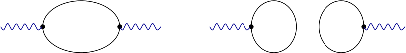
Figure 1: Quark line diagrams that contribute to the vector and axial-vector two-point function in the iso-vector and iso-singlet channel. The solid lines denote quark propagators in a gluonic background field. The two diagrams show the connected and disconnected contribution.

The iso-singlet correlator receives additional, disconnected, contributions, see Fig. 1. The iso-singlet vector ($\omega$) correlator is given by

$$(\Pi_{V}^{0})_{\mu\nu}(x,y)=2(P^{con}_{V})_{\mu\nu}(x,y)+4(P^{dis}_{V})_{\mu\nu}(x,y)$$ (26)

with

$$(P^{dis}_{V})_{\mu\nu}(x,y)=\langle{\rm Tr}\left[\gamma_{\mu}S(x,x)\right]{\rm Tr}\left[\gamma_{\nu}S(y,y)\right]\rangle.$$ (27)

The axial-vector correlation functions are defined analogously. At very short distance the correlation functions are dominated by the free quark contribution $\Pi_{A}^{3}=\Pi_{A}^{0}=\Pi_{V}^{3}=\Pi_{V}^{0}\sim 1/x^{6}$. Perturbative corrections to the connected correlators are $O(\alpha_{s}(x)/\pi)$, but perturbative corrections to the disconnected correlators are very small, $O((\alpha_{s}(x)/\pi)^{2})$. In this section we will compute the instanton contribution to the correlation functions. At short distance, it is sufficient to consider a single instanton. For the connected correlation functions, this calculation was first performed by Andrei and Gross Andrei:xg , see also Nason:1993ak . Disconnected correlation function were first considered in Geshkenbein:vb and a more recent study can be found in Dorokhov:2003kf .

In order to make contact with our calculation of the vector and axial-vector three-point functions in the next section, we briefly review the calculation of Andrei and Gross, and then compute the disconnected contribution. Using the expansion in powers of the quark mass, equ. (13), we can write

$$(P^{con}_{V})_{\pm}^{\mu\nu}(x,y)=(P^{con}_{V})^{\mu\nu}_{0}+A^{\mu\nu}_{\pm}+B^{\mu\nu}_{\pm}$$ (28)

with

$$(P_{V}^{con})^{\mu\nu}_{0} = -{\rm Tr}\left[\gamma^{\mu}S_{0}(x,y)\gamma^{\nu}S_{0}(y,x)\right],$$ (29)

$$A^{\mu\nu}_{\pm} = -{\rm Tr}\left[\gamma^{\mu}S^{NZ}_{\pm}(x,y)\gamma^{\nu}S^{NZ}_{\pm}(y,x)\right]-(P^{con}_{V})_{0}^{\mu\nu}(x,y),$$ (30)

$$B^{\mu\nu}_{\pm} = -2{\rm Tr}\left[\gamma^{\mu}\Psi_{0\pm}(x)\Psi_{0\pm}^{+}(y)\gamma^{\nu}\Delta_{\pm}(y,x)\gamma_{\pm}\right].$$ (31)

Using the explicit expression for the propagators given in the previous section we find

$$A^{\mu\nu}_{\pm} = \frac{\rho^{2}h_{x}h_{y}}{2\pi^{4}\Delta^{4}}\left\{S^{\mu\alpha\nu\beta}\Big{[}\rho^{2}h_{x}h_{y}(2\Delta_{\alpha}\Delta_{\beta}-\Delta^{2}\delta_{\alpha\beta})+h_{y}(y_{\beta}\Delta_{\alpha}+y_{\alpha}\Delta_{\beta})\right.$$ (32)

$$\hskip 56.9055pt\mbox{}\left.-h_{x}(x_{\beta}\Delta_{\alpha}+x_{\alpha}\Delta_{\beta})\Big{]}\mp 2\epsilon^{\mu\nu\alpha\beta}(h_{y}\Delta_{\alpha}y_{\beta}-h_{x}\Delta_{\beta}x_{\alpha})\right\}$$

and

$$B^{\mu\nu}_{\pm}=-\frac{\rho^{2}}{\pi^{4}\Delta^{2}}h_{x}^{2}h_{y}^{2}\left\{(x\cdot y+\rho^{2})\delta^{\mu\nu}-(y^{\mu}x^{\nu}-x^{\mu}y^{\nu})\mp\epsilon^{\mu\alpha\nu\beta}x_{\alpha}y_{\beta}\right\}$$ (33)

with $h_{x}=1/(x^{2}+\rho^{2})$, $\Delta=x-y$, and $S^{\mu\alpha\nu\beta}=g^{\mu\alpha}g^{\nu\beta}-g^{\mu\nu}g^{\alpha\beta}+g^{\mu\beta}g^{\alpha\nu}$. Our result agrees with Andrei:xg up to a color factor of $3/2$, first noticed in Dubovikov:bf , a ’-’ sign in front of the epsilon terms, which cancels after adding instantons and anti-instantons, and a ’-’ sign in front of the 2nd term in $B^{\mu\nu}$. This sign is important in order to have a conserved current, but it does not affect the trace $P^{\mu\mu}$. Summing up the contributions from instantons and anti-instantons we obtain

$$(P^{con}_{V})^{\mu\nu}(x,y) = 2\frac{12S^{\mu\alpha\nu\beta}\Delta_{\alpha}\Delta_{\beta}}{(2\pi^{2})^{2}\Delta^{8}}+\frac{1}{2\pi^{4}}(h_{x}h_{y})^{2}\rho^{2}\left[-\frac{2\Sigma^{2}}{\Delta^{4}}\Delta^{\mu}\Delta^{\nu}+\frac{2\Sigma\cdot\Delta}{\Delta^{4}}(\Sigma^{\mu}\Delta^{\nu}+\Delta^{\mu}\Sigma^{\nu}\right.$$ (34)

$$\hskip 56.9055pt\mbox{}\left.-\Sigma\cdot\Delta g^{\mu\nu})+\frac{2}{\Delta^{2}}(\Delta^{2}g^{\mu\nu}-\Delta^{\mu}\Delta^{\nu}-\Delta^{\mu}\Sigma^{\nu}+\Delta^{\nu}\Sigma^{\mu})\right].$$

This result has to be averaged over the position of the instanton. We find

$$2a^{\mu\nu} = \sum_{\pm}\int d^{4}zA^{\mu\nu}_{\pm}(x-z,y-z)=-\frac{1}{\pi^{2}}\left[\frac{\partial^{2}}{\partial\Delta_{\mu}\partial\Delta_{\nu}}G(\Delta^{2},\rho)+2G^{\prime}(\Delta^{2},\rho)g^{\mu\nu}\right],$$ (35)

$$2b^{\mu\nu} = \sum_{\pm}\int d^{4}zB^{\mu\nu}_{\pm}(x-z,y-z)=\frac{1}{\pi^{2}}\left[\frac{\partial^{2}}{\partial\Delta^{2}}G(\Delta^{2},\rho)+2G^{\prime}(\Delta^{2},\rho)\right]g^{\mu\nu},$$ (36)

with

$$G^{\prime}(\Delta^{2},\rho)=\frac{\partial G(\Delta^{2},\rho)}{\partial\Delta^{2}}=\frac{\rho^{2}}{\Delta^{4}}\left[-\frac{2\rho^{2}}{\Delta^{2}}\xi\log\frac{1-\xi}{1+\xi}-1\right]$$ (37)

and $\xi^{2}=\Delta^{2}/(\Delta^{2}+4\rho^{2})$. The final result for the single instanton contribution to the connected part of the vector current correlation function is

$$\delta(P_{V}^{con})^{\mu\mu}=(P_{V}^{con})^{\mu\mu}-2(P^{con}_{V})^{\mu\mu}_{0}=\frac{24}{\pi^{2}}\frac{\rho^{4}}{\Delta^{2}}\;\frac{\partial}{\partial\Delta^{2}}\left(\frac{\xi}{\Delta^{2}}\log\frac{1+\xi}{1-\xi}\right)\equiv\frac{24}{\pi^{2}}\frac{\rho^{4}}{\Delta^{2}}F(\Delta,\xi),$$ (38)

where we defined

$$F(\Delta,\xi)=\frac{\partial}{\partial\Delta^{2}}\left(\frac{\xi}{\Delta^{2}}\log\frac{1+\xi}{1-\xi}\right).$$ (39)

The computation of the connected part of the axial-vector correlator is very similar. Using equs. (30,31) we observe that the only difference is the sign in front of $B^{\mu\nu}$. We find

$$\delta(P^{con}_{A})^{\mu\mu}=(P^{con}_{A})^{\mu\mu}-2(P^{con}_{A})^{\mu\mu}_{0}=-\frac{1}{\pi^{2}}\left[20\Delta^{2}G^{\prime\prime}+56G^{\prime}\right],$$ (40)

with $G^{\prime}$ given in equ. (37)

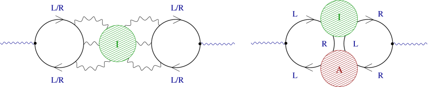
Figure 2: Instanton contributions to the disconnected axial-vector correlation function. The left panel shows the single-instanton (non-zero mode) contribution. The right panel shows the instanton-anti-instanton (fermion zero mode) contribution.

We now come to the disconnected part, see Fig. 2. In the vector channel the single instanton contribution to the disconnected correlator vanishes Geshkenbein:vb . In the axial-vector channel we can use the result for ${\rm Tr}[\gamma_{5}\gamma^{\mu}S(x,x)]$ derived in the previous section. The correlation function is

$$(P^{dis}_{A})^{\mu\nu}(x,y)=\frac{4\rho^{4}(x-z)^{\mu}(y-z)^{\nu}}{\pi^{4}((x-z)^{2}+\rho^{2})^{3}((y-z)^{2}+\rho^{2})^{3}}.$$ (41)

Summing over instantons and anti-instantons and integrating over the center of the instanton gives

$$(P^{dis}_{A})^{\mu\nu}=2\frac{\rho^{4}}{2\pi^{2}}\frac{\partial^{2}}{\partial\Delta_{\mu}\partial\Delta_{\nu}}F(\Delta,\xi)$$ (42)

and

$$(P^{dis}_{A})^{\mu\mu}=\frac{4\rho^{4}}{\pi^{2}}\left\{2\frac{d}{d\Delta^{2}}+\Delta^{2}\left(\frac{d}{d\Delta^{2}}\right)^{2}\right\}F(\Delta,\xi).$$ (43)

We can now summarize the results in the vector singlet ($\omega$) and triplet ($\rho$), as well as axial-vector singlet ($f_{1}$) and triplet ($a_{1}$) channel. The result in the $\rho$ and $\omega$ channel is

$$(\Pi^{3}_{V})^{\mu\mu}=(\Pi^{0}_{V})^{\mu\mu}=-\frac{12}{\pi^{4}\Delta^{6}}+2\int d\rho n(\rho)\frac{24}{\pi^{2}}\frac{\rho^{4}}{\Delta^{2}}F(\Delta,\xi).$$ (44)

In the $a_{1},f_{1}$ channel we have

$$(\Pi^{3}_{A})^{\mu\mu} = -\frac{12}{\pi^{4}\Delta^{6}}+\int d\rho n(\rho)\left[-\frac{2}{\pi^{2}}\left(20\Delta^{2}G^{\prime\prime}+56G^{\prime}\right)\right],$$ (45)

$$(\Pi^{0}_{A})^{\mu\mu} = -\frac{12}{\pi^{4}\Delta^{6}}+\int d\rho n(\rho)\left[-\frac{2}{\pi^{2}}\left(20\Delta^{2}G^{\prime\prime}+56G^{\prime}\right)+\frac{16\rho^{4}}{\pi^{2}}\left(2F^{\prime}+\Delta^{2}F^{\prime\prime}\right)\right].$$ (46)

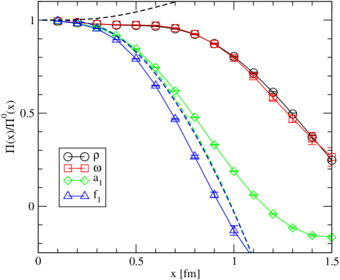
Figure 3: Correlation functions in the $\rho,\omega,a_{1}$ and $f_{1}$ channel. All correlation functions are normalized to free field behavior. The data points show results from a numerical simulation of the random instanton liquid. The dashed lines show the single instanton approximation.

In order to obtain a numerical estimate of the instanton contribution we use a very simple model for the instanton size distribution, $n(\rho)=n_{0}\delta(\rho-\bar{\rho})$, with $\bar{\rho}=0.3$ fm and $n_{0}=0.5\,{\rm fm}^{-4}$. The results are shown in Fig. 3.

We observe that the OZI rule violating difference between the singlet and triplet axial-vector correlation functions is very small and repulsive. We can also see this by studying the short distance behavior of the correlation functions. The non-singlet correlators satisfy

$$(\Pi_{V}^{3})^{\mu\mu} = (\Pi_{V}^{3})^{\mu\mu}_{0}\left\{1+\frac{\pi^{2}x^{4}}{3}\int d\rho n(\rho)+\ldots\right\},$$ (47)

$$(\Pi_{A}^{3})^{\mu\mu} = (\Pi_{A}^{3})^{\mu\mu}_{0}\left\{1-\pi^{2}x^{4}\int d\rho n(\rho)+\ldots\right\}.$$ (48)

As explained by Dubovikov and Smilga, this result can be understood in terms of the contribution of the dimension $d=4$ operators $\langle g^{2}G^{2}\rangle$ and $\langle m\bar{q}q\rangle$ in the operator product expansion (OPE). The OZI violating contribution

$$(\Pi^{OZI}_{A})^{\mu\mu}=(\Pi^{0}_{A})^{\mu\mu}-(\Pi^{3}_{A})^{\mu\mu}=-(\Pi^{3}_{A})^{\mu\mu}_{0}\left(\frac{4\pi^{2}}{45}\frac{x^{6}}{\rho^{2}}\right)\int d\rho n(\rho)$$ (49)

is of $O(x^{6})$ and not singular at short distance. Our results show that it remains small and repulsive even if $x>\rho$. We also note that the sign of the OZI-violating term at short distance is model independent. The quark propagator in euclidean space satisfies the Weingarten relation

$$S(x,y)^{\dagger}=\gamma_{5}S(y,x)\gamma_{5}.$$ (50)

This relation implies that ${\rm Tr}[S(x,x)\gamma_{\mu}\gamma_{5}]$ is purely real. As a consequence we have

$$\lim_{x\to y}\Big{\{}{\rm Tr}[S(x,x)\gamma_{\mu}\gamma_{5}]{\rm Tr}[S(y,y)\gamma_{\mu}\gamma_{5}]\Big{\}}>0.$$ (51)

Since the path integral measure in euclidean space is positive this inequality translates into an inequality for the correlation functions. In our convention the trace of the free correlation function is negative, and equ. (51) implies that the interaction is repulsive at short distance. The result is in agreement with the single instanton calculation.

We can also study higher order corrections to the single instanton result. The two-instanton (anti-instanton) contributions is of the same form as the one-instanton result. An interesting contribution arises from instanton-anti-instanton pairs, see Fig. 2. This effect was studied in Schafer:1994nv . It was shown that the instanton-anti-instanton contribution to the disconnected meson channels can be described in terms of an effective lagrangian

$${\cal L}=\frac{2G}{N_{c}^{2}}(\bar{\psi}\gamma_{\mu}\gamma_{5}\psi)^{2}$$ (52)

with

$$G=\int d\rho_{1}d\rho_{2}(2\pi\rho_{1})^{2}(2\pi\rho_{2})^{2}\frac{n(\rho_{1},\rho_{2})}{8T_{IA}^{2}}$$ (53)

where $n(\rho_{1},\rho_{2})$ is the tunneling rate for an instanton-anti-instanton pair and $T_{IA}$ is the matrix element of the Dirac between the two (approximate) zero modes. We note that this interaction is also repulsive, and that there is no contribution to the $\omega$ channel.

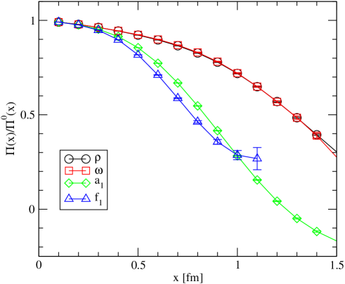
Figure 4: Correlation functions in the $\rho,\omega,a_{1}$ and $f_{1}$ channel. All correlation functions are normalized to free field behavior. The data points show results from unquenched simulations of the instanton liquid model.

Numerical results for the vector meson correlation functions are shown in Figs. 3 and 4. The correlation functions are obtained from Monte Carlo simulations of the instanton liquid as described in Schafer:1995pz ; Schafer:1995uz . We observe that OZI violation in the vector channel is extremely small, both in quenched and unquenched simulations. The OZI violating contribution to the $f_{1}$ channel is repulsive. In quenched simulations this contribution becomes sizable at large distance. Most likely this is due to mixing with an $\eta^{\prime}$ ghost pole. We observe that the effect disappears in unquenched simulations. The pion contribution to the $a_{1}$ correlator is of course present in both quenched and unquenched simulations.

Experimentally we know that the $\rho$ and $\omega$, as well as the $a_{1}$ and $f_{1}$ meson, are indeed almost degenerate. Both iso-singlet states are slightly heavier than their iso-vector partners. To the best of our knowledge there has been only one attempt to measure OZI violating correlation functions in the vector and axial-vector channel on the lattice, see Isgur:2000ts . Isgur and Thacker concluded that OZI violation in both channels was too small to be reliably measurable in their simulation.

IV Axial Vector Coupling of a Quark

In this section we wish to study the iso-vector and iso-singlet axial coupling of a single quark. Our purpose is twofold. One reason is that the calculation of the axial-vector three-point function involving a single quark is much simpler than that of the nucleon, and that it is closely connected to the axial-vector two-point function studied in the previous section. The second, more important, reason is the success of the constituent quark model in describing many properties of the nucleon. It is clear that constituent quarks have an intrinsic structure, and that the axial decay constant of a constituent quark need not be close to one. Indeed, Weinberg argued that the axial coupling of a quark is $(g_{A}^{3})_{Q}\simeq 0.8$ Weinberg:gf . Using this value of $(g_{A}^{3})_{Q}$ together with the naive $SU(6)$ wave function of the nucleon gives the nucleon axial coupling $g_{A}^{3}=0.8\cdot 5/3\simeq 1.3$, which is a significant improvement over the naive quark model result $5/3$. It is interesting to study whether, in a similar fashion, the suppression of the flavor singlet axial charge takes place on the level of a constituent quark.

In order to address this question we study three-point functions involving both singlet and triplet vector and axial-vector currents. The vector three-point function is

$$(\Pi^{a}_{VQQ})^{\alpha\beta}_{\mu}(x,z,y)=\langle q^{\alpha}(x)V^{a}_{\mu}(z)\bar{q}^{\beta}(y)\rangle.$$ (54)

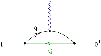
Figure 6: Physical interpretation of the gauge invariant axial-vector three-point function of a quark in terms of a weak light-quark transition in a heavy-light $\bar{Q}q$ meson.

The axial-vector function $(\Pi^{a}_{AQQ})$ is defined analogously. We should note that equ. (54) is not gauge invariant. We can define a gauge invariant correlation function by including a gauge string. The gauge string can be interpreted as the propagator of a heavy anti-quark, see Fig. 6. This implies that the gauge invariant quark axial-vector three-point function is related to light quark weak transitions in heavy-light mesons.

The spectral representation of vector and axial-vector three-point functions is studied in some detail in the appendix. The main result is that in the limit that $y_{4}\gg z_{4}\gg x_{4}$ the ratio

$$\frac{{\rm Tr}[(\Pi^{a}_{AQQ})_{3}\gamma_{5}\gamma_{3}]}{{\rm Tr}[(\Pi^{a}_{VQQ})_{4}\gamma_{4}]}\to\frac{g_{A}}{g_{V}}$$ (55)

tends to the ratio of axial-vector and vector coupling constants, $g_{A}/g_{V}$. We therefore define the following Dirac traces

$$(\Pi^{a}_{VQQ})^{\mu\nu}(x,z,y) = {\rm Tr}[(\Pi^{a}_{VQQ})^{\mu}\gamma^{\nu}],$$ (56)

$$(\Pi^{a}_{AQQ})^{\mu\nu}(x,z,y) = {\rm Tr}[(\Pi^{a}_{AQQ})^{\mu}\gamma_{5}\gamma^{\nu}].$$ (57)

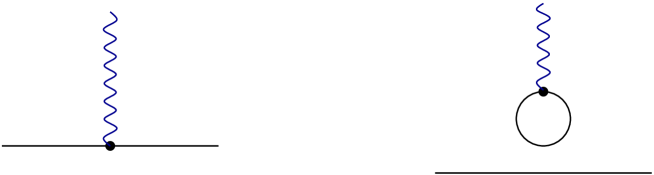
Figure 5: Quark line diagrams that contribute to the vector and axial-vector three-point function of a constituent quark. The solid lines denote quark propagators in a gluonic background field. The two diagrams show the connected and disconnected contribution.

As in the case of the two-point function the iso-triplet correlator only receives quark-line connected contributions, whereas the iso-singlet correlation function has a disconnected contribution, see Fig. 5. We find

$$(\Pi^{3}_{VQQ})^{\mu\nu}(x,z,y)=(P^{con}_{VQQ})^{\mu\nu}(x,z,y)=\langle{\rm Tr}[S(x,z)\gamma^{\mu}S(z,y)\gamma^{\nu}]\rangle$$ (58)

and

$$(\Pi^{0}_{VQQ})^{\mu\nu}(x,z,y)=(P^{con}_{VQQ})^{\mu\nu}(x,z,y)-2(P^{dis}_{VQQ})^{\mu\nu}(x,z,y)$$ (59)

with

$$(P^{dis}_{VQQ})^{\mu\nu}(x,z,y)=\langle{\rm Tr}[S(x,y)\gamma^{\mu}]{\rm Tr}[S(z,z)\gamma^{\nu}]\rangle,$$ (60)

as well as the analogous result for the axial-vector correlator.

In the following we compute the single instanton contribution to these correlation functions. We begin with the connected part. We again write the propagator in the field of the instanton as $S_{ZM}+S_{NZ}+S_{m}$ where $S_{ZM}$ is the zero-mode term, $S_{NZ}$ is the non-zero mode term, and $S_{m}$ is the mass correction. In the three-point correlation function we get contribution of the type $S_{NZ}S_{NZ}$, $S_{ZM}S_{m}$ and $S_{m}S_{ZM}$

$$(P^{con}_{A/VQQ})^{\mu\nu} = P_{NZNZ}^{\mu\nu}+c_{A/V}\left(P^{\mu\nu}_{ZMm}+P^{\mu\nu}_{mZM}\right)$$ (61)

$$= {\rm Tr}[S^{NZ}(x,z)\gamma^{\mu}S^{NZ}(z,y)\gamma^{\nu}]$$

$$+c_{A/V}{\rm Tr}[-\Psi_{0}(x)\Psi_{0}^{+}(z)\gamma^{\mu}(-\Delta_{\pm}(z,y)\gamma_{\pm}\gamma^{\nu}]$$

$$+c_{A/V}{\rm Tr}[(-\Delta_{\pm}(x,z)\gamma_{\pm})\gamma^{\mu}(-\Psi_{0}(z)\Psi_{0}^{+}(y))\gamma^{\nu}],$$

where the only difference between the vector and axial-vector case is the sign of ’ZMm’ and ’mZM’ terms. We have $c_{A/V}=\pm 1$ for vector (axial vector) current insertions. The detailed evaluation of the traces is quite tedious and we relegate the results to the appendix B.

Our main goal is the calculation of the disconnected correlation function, which is related to OZI violation. In the single instanton approximation only the axial-vector correlator receives a non-zero disconnected contribution

$$(P^{dis}_{AQQ})^{\mu\nu}={\rm Tr}[S(x,y)\gamma_{5}\gamma^{\nu}]{\rm Tr}[S(z,z)\gamma_{5}\gamma^{\mu}],$$ (62)

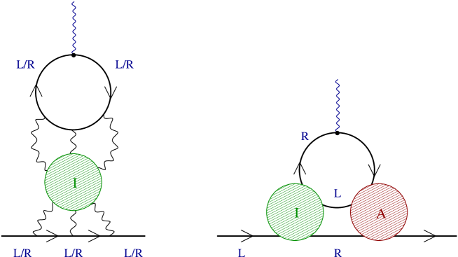
Figure 7: Instanton contributions to the disconnected axial-vector three-point correlation function of a quark. The left panel shows the single-instanton (non-zero mode) contribution. The right panel shows the instanton-anti-instanton (fermion zero mode) contribution.

see Fig. 7. We observe that the second trace is the axial-vector current in the field of an instanton, see equ. (19). As for the first trace, it is easy to see that neither the zero mode part of the propagator nor the part of $S_{NZ}$ proportional to the free propagator can contribute. A straight-forward computation gives

$${\rm Tr}[S(x,y)\gamma_{5}\gamma^{\nu}]=\mp\frac{\rho^{2}}{\pi^{2}(x-y)^{2}x^{2}y^{2}}\frac{x^{\alpha}y^{\beta}(x-y)^{\sigma}}{\sqrt{(1+\frac{\rho^{2}}{x^{2}})(1+\frac{\rho^{2}}{y^{2}})}}\left(\frac{S^{\alpha\nu\sigma\beta}}{\rho^{2}+x^{2}}-\frac{S^{\alpha\sigma\nu\beta}}{\rho^{2}+y^{2}}\right).$$ (63)

Combined with equ. (19) we obtain

$$(P^{dis}_{AQQ})^{\mu\nu}=-\frac{2\rho^{4}z^{\mu}x^{\alpha}y^{\beta}(x-y)^{\sigma}}{\pi^{4}(x-y)^{2}x^{2}y^{2}(z^{2}+\rho^{2})^{3}}\frac{1}{\sqrt{(1+\frac{\rho^{2}}{x^{2}})(1+\frac{\rho^{2}}{y^{2}})}}\left(\frac{S^{\alpha\nu\sigma\beta}}{\rho^{2}+x^{2}}-\frac{S^{\alpha\sigma\nu\beta}}{\rho^{2}+y^{2}}\right),$$ (64)

which has to be multiplied by a factor 2 in order to take into account both instantons and anti-instantons.

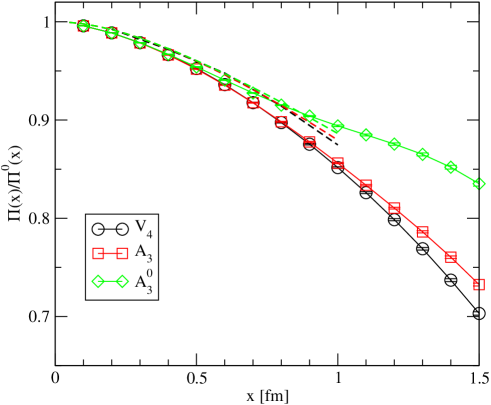
Figure 8: Axial and vector three-point functions of a quark as a function of the separation between the two quark sources. The correlation functions are normalized to free field behavior. The data points show results from numerical simulations of the instanton liquid and the dashed lines show the single instanton approximation.

Results for the vector and axial-vector three-point functions $(\Pi_{VQQ}^{3})^{44}(\tau,\tau/2,0)$ and $(\Pi_{AQQ}^{0,3})^{33}(\tau,\tau/2,0)$ are shown in Fig. 8. We observe that the vector and axial-vector correlation functions are very close to one another. We also note that the disconnected contribution adds to the connected part of the axial-vector three-point function. This can be understood from the short distance behavior of the correlation function. The disconnected part of the gauge invariant three-point function satisfies

$$\lim_{y,z\to x}\Big{\{}(\Pi_{AQQ}^{dis})^{33}(x,z,y)\Big{\}}=\lim_{x\to z}\Big{\{}{\rm Tr}[S(x,x)\gamma_{3}\gamma_{5}]{\rm Tr}[S(z,z)\gamma_{3}\gamma_{5}]\Big{\}}>0.$$ (65)

This expression is exactly equal to the short distance term in the disconnected $f_{1}$ meson correlation function. The short distance behavior of the connected three-point function, on the other hand, is opposite in sign to the two-point function. This is related to the fact that the two-point function involves one propagator in the forward direction and one in the backward direction, whereas the three-point function involves two forward propagating quarks. A similar connection between the interaction in the $f_{1}$ meson channel and the flavor singlet coupling of a constituent quark was found in a Nambu-Jona-Lasinio model Vogl:1991qt ; Steininger:ed . It was observed, in particular, that an attractive coupling in the $f_{1}$ channel is needed in order to suppress the flavor singlet $(g_{A}^{0})_{Q}$.

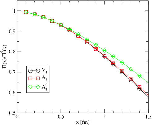
Figure 9: Axial and vector three-point functions of a quark as a function of the separation between the two quark sources. The data points show results from an unquenched instanton simulation.

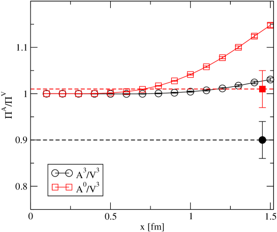
Figure 10: Ratio of axial-vector to vector correlation functions of a constituent quark calculated in the instanton liquid model. The open points show point-to-point correlation functions while the solid point is the zero momentum (point-to-plane) limit. The figure shows the iso-vector and iso-singlet correlation functions.

The same general arguments apply to the short distance contribution from instanton-anti-instanton pairs. At long distance, on the other hand, we expect that IA pairs reduce the flavor singlet axial current correlation function. The idea can be understood from Fig. 7, see Dorokhov:ym ; Dorokhov:2001pz ; Kochelev:1997ux . In an IA transition a left-handed valence up quark emits a right handed down quark which acts to shield its axial charge. We have studied this problem numerically, see Figs. 8-10. We find that in quenched simulations the flavor singlet axial three-point function is significantly enhanced. This effect is analogous to what we observed in the $f_{1}$ channel and disappears in unquenched simulations. We have also studied the axial three-point function at zero three-momentum $\vec{q}=0$. This correlation function is directly related to the coupling constant, see App. A. We find that the iso-vector coupling is smaller than one, $(g_{A}^{3})_{Q}\simeq 0.9$, in agreement with Weinberg’s idea. The flavor singlet coupling, on the other hand, is close to one. We observe no suppression of the singlet charge of a constituent quark. We have also checked that this result remains unchanged in unquenched simulations.

V Axial Structure of the Nucleon

In this section we shall study the axial charge of the nucleon in the instanton model. We consider the same correlation functions as in the previous section, but with the quark field replaced by a nucleon current. The vector three-point function is given by

$$(\Pi^{a}_{VNN})^{\alpha\beta}_{\mu}(x,y)=\langle\eta^{\alpha}(0)V^{a}_{\mu}(y)\bar{\eta}^{\beta}(x)\rangle.$$ (66)

Here, $\eta^{\alpha}$ is a current with the quantum numbers of the nucleon. Three-quark currents with the nucleon quantum numbers were introduced by Ioffe Ioffe:kw . He showed that there are two independent currents with no derivatives and the minimum number of quark fields that have positive parity and spin $1/2$. In the case of the proton, the two currents are

$$\eta_{1}=\epsilon_{abc}(u^{a}C\gamma_{\mu}u^{b})\gamma_{5}\gamma_{\mu}d^{c},\hskip 28.45274pt\eta_{2}=\epsilon_{abc}(u^{a}C\sigma_{\mu\nu}u^{b})\gamma_{5}\sigma_{\mu\nu}d^{c}.$$ (67)

It is sometimes useful to rewrite these currents in terms of scalar and pseudo-scalar diquark currents. We find

$$\eta_{1} = 2\left\{\epsilon_{abc}(u^{a}Cd^{b})\gamma_{5}u^{c}-\epsilon_{abc}(u^{a}C\gamma_{5}d^{b})u^{c}\right\},$$ (68)

$$\eta_{2} = 4\left\{\epsilon_{abc}(u^{a}Cd^{b})\gamma_{5}u^{c}+\epsilon_{abc}(u^{a}C\gamma_{5}d^{b})u^{c}\right\}.$$ (69)

Instantons induce a strongly attractive interaction in the scalar diquark channel $\epsilon^{abc}(u^{b}C\gamma_{5}d^{c})$ Schafer:1993ra ; Rapp:1997zu . As a consequence, the nucleon mainly couples to the scalar diquark component of the Ioffe currents $\eta_{1,2}$. This phenomenon was also observed on the lattice Leinweber:1994nm . This result is suggestive of a model of the spin structure that is quite different from the naive quark model. In this picture the nucleon consists of a tightly bound scalar-isoscalar diquark, loosely coupled to the third quark Anselmino:1992vg . The quark-diquark model suggests that the spin and isospin of the nucleon are mostly carried by a single constituent quark, and that $g_{A}^{N}\simeq g_{A}^{Q}$.

Nucleon correlation functions are defined by $\Pi^{N}_{\alpha\beta}(x)=\langle\eta_{\alpha}(0)\bar{\eta}_{\beta}(x)\rangle$, where $\alpha,\beta$ are Dirac indices. The correlation function of the first Ioffe current is

$$\Pi_{\alpha\beta}(x)=2\epsilon_{abc}\epsilon_{a^{\prime}b^{\prime}c^{\prime}}\,\langle\left(\gamma_{\mu}\gamma_{5}S_{d}^{cc^{\prime}}(0,x)\gamma_{\nu}\gamma_{5}\right)_{\alpha\beta}\,{\rm Tr}\left[\gamma_{\mu}S_{u}^{aa^{\prime}}(0,x)\gamma_{\nu}C(S_{u}^{bb^{\prime}}(0,x))^{T}C\right]\rangle.$$ (70)

The vector and axial-vector three-point functions can be constructed in terms of vector and axial-vector insertions into the quark propagator,

$$(\Gamma^{V}_{\mu})_{f}^{aa^{\prime}}(x,y) = S_{f}^{ab}(0,y)\gamma_{\mu}S_{f}^{ba^{\prime}}(y,x),$$ (71)

$$(\Gamma^{A}_{\mu})_{f}^{aa^{\prime}}(x,y) = S_{f}^{ab}(0,y)\gamma_{\mu}\gamma_{5}S_{f}^{ba^{\prime}}(y,x).$$ (72)

The three-point function is given by all possible substitutions of equ. (71) and (72) into the two-point function. We have

$$\begin{array}[]{rclc}(\Pi^{a}_{VNN})^{\alpha\beta}_{\mu}(x,y)=2\epsilon_{abc}\epsilon_{a^{\prime}b^{\prime}c^{\prime}}&&&\\ \langle\Bigg{\{}&g_{V}^{d}\left(\gamma_{\rho}\gamma_{5}(\Gamma^{V}_{\mu})_{d}^{cc^{\prime}}(x,y)\gamma_{\sigma}\gamma_{5}\right)_{\alpha\beta}&{\rm Tr}\left[\gamma_{\rho}S_{u}^{aa^{\prime}}(0,x)\gamma_{\sigma}C(S_{u}^{bb^{\prime}}(0,x))^{T}C\right]&\\ +&2g_{V}^{u}\left(\gamma_{\rho}\gamma_{5}S_{d}^{cc^{\prime}}(0,x)\gamma_{\sigma}\gamma_{5}\right)_{\alpha\beta}&{\rm Tr}\left[\gamma_{\rho}(\Gamma^{V}_{\mu})_{u}^{aa^{\prime}}(x,y)\gamma_{\sigma}C(S_{u}^{bb^{\prime}}(0,x))^{T}C\right]&\\ -&\left(\gamma_{\rho}\gamma_{5}S_{d}^{cc^{\prime}}(0,x)\gamma_{\sigma}\gamma_{5}\right)_{\alpha\beta}&{\rm Tr}\left[\gamma_{\rho}S_{u}^{aa^{\prime}}(0,x)\gamma_{\sigma}C(S_{u}^{bb^{\prime}}(0,x))^{T}C\right]&\\ &&\cdot\;{\rm Tr}\left[g_{V}^{u}\gamma_{\mu}S_{u}^{dd}(y,y)+g_{V}^{d}\gamma_{\mu}S_{d}^{dd}(y,y)\right]&\Bigg{\}}\rangle,\end{array}$$ (73)

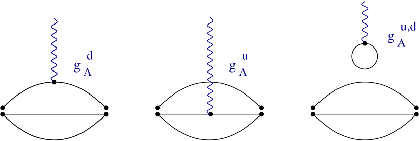
Figure 11: Quark line diagrams that contribute to the axial-vector three-point function of the proton. The solid lines denote quark propagators in a gluonic background field. The lines are connected in the same way that the Dirac indices of the propagators are contracted. The iso-vector and iso-singlet correlation functions correspond to $g_{A}^{u}=-g_{A}^{d}=1$ and $g_{A}^{u}=g_{A}^{d}=1$, respectively. The disconnected diagram only contributes to the iso-scalar three-point function.

where the first term is the vector insertion into the $d$ quark propagator in the proton, the second term is the insertion into the $uu$ diquark, and the third term is the disconnected contribution, see Fig. 11. The vector charges of the quarks are denoted by $g_{V}^{f}$. In the case of the iso-vector three-point function we have $g_{V}^{u}=1$, $g_{V}^{d}=-1$ and in the iso-scalar case $g_{V}^{u}=g_{V}^{d}=1$.

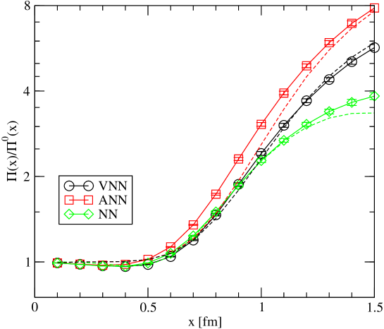
Figure 12: Vector, axial-vector three-point functions of the nucleon and nucleon two-point function calculated in the instanton liquid model. All correlation functions are normalized to free field behavior. The results are compared to a simple pole fit of the type discussed in the appendix.

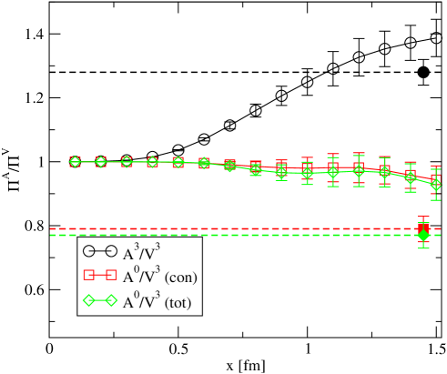
Figure 13: Ratio of axial-vector to vector correlation functions of the nucleon calculated in the instanton liquid model. The open points show point-to-point correlation functions while the solid point is the zero momentum (point-to-plane) limit. The figure shows the iso-vector, connected iso-singlet, and full iso-singlet axial-vector correlation functions.

Vector and axial-vector three-point functions of the nucleon are shown in Figs. 12 and 13. In order to verify that the correlation functions are dominated by the nucleon pole contribution we have compared our results to the spectral representation discussed in the appendix, see Fig. 12. The nucleon coupling constant was determined from the nucleon two-point function. The figure shows that we can describe the three-point functions using the phenomenological values of the vector and axial-vector coupling constants. We have also checked that the ratio of axial-vector and vector current three-point functions is independent of the nucleon interpolating field for $x>1$ fm. The only exception is a pure pseudo-scalar diquark current, which has essentially no overlap with the nucleon wave function.

The main result is that the iso-vector axial-vector correlation function is larger than the vector correlator. The corresponding ratio is shown in Fig. 13, together with the ratio of $\vec{q}=0$ correlation functions. We find that the iso-vector axial coupling constant is $g_{A}^{3}=1.28$, in good agreement with the experimental value. We also observe that the ratio of point-to-point correlation functions is larger than this value. As explained in the appendix, this shows that the axial radius of the nucleon is smaller than the vector radius. Taking into account only the connected part of the correlation function we find a singlet coupling $g_{A}^{0}=0.79$. The disconnected part is very small, $g_{A}^{0}(dis)=-(0.02\pm 0.02)$. Assuming that $\Delta s\simeq\Delta u(dis)=\Delta d(dis)$ this implies that the OZI violating difference $g_{A}^{8}-g_{A}^{0}$ is small. This result does not change in going from the quenched approximation to full QCD.

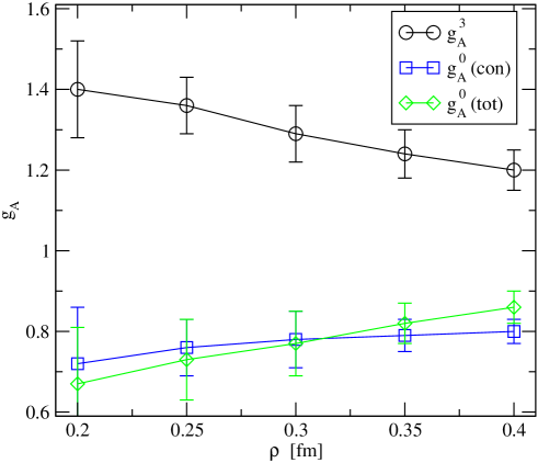
Figure 14: Axial coupling constants of the nucleon as a function of the instanton size $\rho$ with the instanton density fixed at $(N/V)=1\,{\rm fm}^{-4}$. We show the iso-vector, connected iso-singlet, and full iso-singlet axial coupling constant.

We have also studied the dependence of the results on the average instanton size, see Fig. 14. We observe that there is a slight decrease in the iso-singlet coupling and a small increase in the iso-vector coupling as the instanton size is decreased. What is surprising is that the disconnected term changes sign between $\rho=0.3$ fm and $\rho=0.35$ fm. The small value $g_{A}^{0}(dis)=-(0.02\pm 0.02)$ obtained above is related to the fact that the phenomenological value of the instanton size is close to the value where $g_{A}^{0}(dis)$ changes sign. However, even for $\rho$ as small as 0.2 fm the disconnected contribution to the axial coupling $g_{A}^{0}(dis)=-(0.05\pm 0.02)$ is smaller in magnitude than phenomenology requires.

VI Conclusions

The main issue raised by the EMC measurement of the flavor singlet axial coupling is not so much why $g_{A}^{0}$ is much smaller than one - except for the naive quark model there is no particular reason to expect $g_{A}^{0}$ to be close to one - but why the OZI violating observable $g_{A}^{0}-g_{A}^{8}$ is large. Motivated by this question we have studied the contribution of instantons to OZI violation in the axial-vector channel. We considered the $f_{1}-a_{1}$ meson splitting, the flavor singlet and triplet axial coupling of a constituent quark, and the axial coupling constant of the nucleon. We found that instantons provide a short distance contribution which is repulsive in the $f_{1}$ meson channel and adds to the gauge invariant flavor singlet three-point function of a constituent quark. We showed that the sign of this term is fixed by positivity arguments.

We computed the axial coupling constants of the constituent quark and the nucleon using numerical simulations of the instanton liquid. We find that the iso-vector axial coupling constant of a constituent quark is $(g_{A}^{3})_{Q}=0.9$ and that of a nucleon is $g_{A}^{3}=1.28$, in good agreement with experiment. The result is also in qualitative agreement with the constituent quark model relation $g_{A}^{3}=5/3\cdot(g_{A}^{3})_{Q}$. The flavor singlet coupling of quark is close to one, while that of a nucleon is suppressed, $g_{A}^{0}=0.77$. However, this value is still significantly larger than the experimental value $g_{A}^{0}=(0.28-0.41)$. In addition to that, we find very little OZI violation, $\Delta s\simeq\Delta u(dis)\simeq-0.01$. We observed, however, that larger values of the disconnected contribution can be obtained if the average instanton size is smaller than the phenomenological value of $\rho\simeq 1/3$ fm.

There are many questions that remain to be addressed. In order to understand what is missing in our calculation it would clearly be useful to perform a systematic study of OZI violation in the axial-vector channel on the lattice. The main question is whether the small value of $g_{A}^{0}$ is a property of the nucleon, or whether large OZI violation is also seen in other channels. A study of the connected contributions to the axial coupling constant in cooled as well as quenched quantum QCD configurations was performed in Dolgov:1998js . These authors find $g_{A}^{0}(con)=\Delta u(con)+\Delta d(con)\simeq 0.6$ in both cooled and full configurations. The disconnected term was computed by Dong et al. Dong:1995rx . They find $\Delta u(dis)+\Delta d(dis)\simeq-0.24$.

In the context of the instanton model it is important to study whether the results for $g_{A}^{0}$ obtained from the axial-vector current three-point function are consistent with calculations of $g_{A}^{0}$ based on the matrix element of the topological charge density $G\tilde{G}$ Forte:1990xb ; Hutter:1995cs ; Kacir:1996qn ; Diakonov:1995qy . It would also be useful to further clarify the connection of the instanton liquid model to soliton models of the nucleon Diakonov:1987ty . In soliton models the spin of the nucleon is mainly due to the collective rotation of the pion cloud, and a small value for $g_{A}^{0}$ is natural Brodsky:1988ip ; Blotz:1993am . The natural parameter that can be used in order to study whether this picture is applicable is the number of colors, $N_{c}$. Unfortunately, a direct calculations of nucleon properties for $N_{c}>3$ would be quite involved. Finally it would be useful to study axial form factors of the nucleon. It would be interesting to see whether there is a significant difference between the iso-vector and iso-singlet axial radius of the nucleon. A similar study of the vector form factors was recently presented in Faccioli:2003yy .

Acknowledgments: We would like to thank E. Shuryak for useful discussions. This work was supported in part by US DOE grant DE-FG-88ER40388.

Appendix A Spectral Representation

A.1 Nucleon Two-Point Function

Consider the euclidean correlation function

$$\Pi^{\alpha\beta}_{N}(x)=\langle\eta^{\alpha}(0)\bar{\eta}^{\beta}(x)\rangle,$$ (74)

where $\eta^{\alpha}(x)$ is a nucleon current and $\alpha$ is a Dirac index. We can write

$$\Pi^{\alpha\beta}_{N}(x)=\Pi_{1}(x)(\hat{x}\cdot\gamma)^{\alpha\beta}+\Pi_{2}(x)\delta^{\alpha\beta}.$$ (75)

The functions $\Pi_{1,2}(x)$ have spectral representations

$$\Pi_{1}(x) = \int_{0}^{\infty}ds\,\rho_{1}(s)D^{\prime}(\sqrt{s},x),$$ (76)

$$\Pi_{2}(x) = \int_{0}^{\infty}ds\,\rho_{2}(s)D(\sqrt{s},x),$$ (77)

where $\rho_{1,2}(s)$ are spectral functions and

$$D(m,x) = \;\frac{m}{4\pi^{2}x}K_{1}(mx),$$ (78)

$$D^{\prime}(m,x) = -\frac{m^{2}}{4\pi^{2}x}K_{2}(mx),$$ (79)

are the euclidean coordinate space propagator of a scalar particle with mass $m$ and its derivative with respect to $x$. The contribution to the spectral function arising from a nucleon pole is

$$\rho_{1}(s)=|\lambda^{2}_{N}|\delta(s-m_{N}^{2}),\hskip 28.45274pt\rho_{2}(s)=|\lambda^{2}_{N}|m_{N}\delta(s-m_{N}^{2}),$$ (80)

where $\lambda_{N}$ is the coupling of the nucleon to the current, $\langle 0|\eta|N(p)\rangle=\lambda_{N}u(p)$, and $m_{N}$ is the mass of the nucleon. It is often useful to consider the point-to-plane correlation function

$$K^{\alpha\beta}_{N}(\tau)=\int d^{3}x\,\Pi^{\alpha\beta}_{N}(\tau,\vec{x}).$$ (81)

The integral over the transverse plane insures that all intermediate states have zero three-momentum. The nucleon pole contribution to the point-to-plane correlation function is

$$K^{\alpha\beta}_{N}(\tau)=\frac{1}{2}(1+\gamma_{4})^{\alpha\beta}|\lambda_{N}|^{2}\exp(-m_{N}\tau).$$ (82)

A.2 Scalar Three-Point Functions

Next we consider three-point functions. Before we get to three-point functions of spinor and vector currents we consider a simpler case in which the spin structure is absent. We study the three-point function of two scalar fields $\phi$ and a scalar current $j$. We define

$$\Pi(x,y)=\langle\phi(0)j(y)\phi(x)\rangle.$$ (83)

The spectral representation of the three-point function is complicated and in the following we will concentrate on the contribution from the lowest pole in the two-point function of the field $\phi$. We define the coupling of this state to the field $\phi$ and the current $j$ as

$$\langle 0|\phi(0)|\Phi(p)\rangle = \lambda,$$ (84)

$$\langle\Phi(p^{\prime})|j(0)|\Phi(p)\rangle = F(q^{2}),$$ (85)

where $F(q^{2})$ with $q=p-p^{\prime}$ is the scalar form factor. The pole contribution to the three-point function is

$$\Pi(x,y)=\lambda^{2}\int d^{4}z\,D(m,y+z)F(z)D(m,x-y-z),$$ (86)

where $D(m,x)$ is the scalar propagator and $F(z)$ is the Fourier transform of the form factor. In order to study the momentum space form factor directly it is convenient to integrate over the location of the endpoint in the transverse plane and Fourier transform with respect to the midpoint

$$\int d^{3}x\,\int d^{3}y\,e^{iqy}\langle\phi(0)j(\tau/2,\vec{y})\phi(\tau,\vec{x})\rangle=\frac{\lambda^{2}}{(2m)^{2}}\exp(-m\tau)F(q^{2}).$$ (87)

The correlation function directly provides the form factor for spacelike momenta. Maiani and Testa showed that there is no simple procedure to obtain the time-like form factor from euclidean correlation functions Maiani:ca .

Form factors are often parametrized in terms of monopole, dipole, or monopole-dipole functions

$$F_{M}(q^{2}) = F_{M}(0)\frac{m_{V}^{2}}{Q^{2}+m_{V}^{2}},$$ (88)

$$F_{D}(q^{2}) = F_{D}(0)\left(\frac{m_{V}^{2}}{Q^{2}+m_{V}^{2}}\right)^{2},$$ (89)

$$F_{MD}(q^{2}) = F_{MD}(0)\frac{m_{1}^{2}}{Q^{2}+m_{1}^{2}}\left(\frac{m_{2}^{2}}{Q^{2}+m_{2}^{2}}\right)^{2},$$ (90)

with $Q^{2}=-q^{2}$. For these parametrization the Fourier transform to euclidean coordinate space can be performed analytically. We find

$$F_{M}(x) = m_{V}^{2}D(x,m_{V})$$ (91)

$$F_{D}(x) = m_{V}^{2}\left(-\frac{x}{2}D^{\prime}(x,m_{V})-D(x,m_{V})\right)$$ (92)

$$F_{MD}(x) = \frac{m_{1}^{2}m_{2}^{4}}{m_{2}^{2}-m_{1}^{2}}\left\{\frac{1}{m_{2}^{2}-m_{1}^{2}}\left(D(x,m_{1})-D(x,m_{2})\right)\right.$$ (93)

$$\left.\hskip 56.9055pt\mbox{}+\frac{1}{m_{2}^{2}}\left(\frac{x}{2}D^{\prime}(x,m_{2})+D(x,m_{2})\right)\right\}.$$

We also consider three-point functions involving a vector current $j_{\mu}$. The matrix element is

$$\langle\Phi(p^{\prime})|j_{\mu}(0)|\Phi(p)\rangle=q_{\mu}F(q^{2}).$$ (94)

The pole contribution to the vector current three-point function is

$$\Pi_{\mu}(x,y)=\lambda^{2}\int d^{4}z\,D(m,y+z)\hat{z}_{\mu}F^{\prime}(z)D(m,x-y-z),$$ (95)

with $F^{\prime}(z)=dF(z)/dz$ and $\hat{z}_{\mu}=z_{\mu}/|z|$. For the parameterizations given above the derivative of the coordinate space form factor can be computed analytically. We get

$$F_{M}^{\prime}(x) = m_{V}^{2}D^{\prime}(x,m_{V})$$ (96)

$$F_{D}^{\prime}(x) = -\frac{m_{V}^{4}}{2}D(x,m_{V})$$ (97)

$$F_{MD}^{\prime}(x) = \frac{m_{1}^{2}m_{2}^{4}}{m_{2}^{2}-m_{1}^{2}}\left\{\frac{1}{m_{2}^{2}-m_{1}^{2}}\left(D^{\prime}(x,m_{1})-D^{\prime}(x,m_{2})\right)\right.$$ (98)

$$\left.\hskip 56.9055pt\mbox{}+\frac{x}{2}D(x,m_{2})\right\}.$$

A.3 Three-Point Functions involving nucleons and vector or axial-vector currents

Next we consider three-point functions of the nucleon involving vector and axial-vector currents. The vector three-point function is

$$(\Pi^{a}_{VNN})^{\alpha\beta}_{\mu}(x,y)=\langle\eta^{\alpha}(0)V^{a}_{\mu}(y)\bar{\eta}^{\beta}(x)\rangle.$$ (99)

The axial-vector three-point function is defined analogously. The nucleon pole contribution involves the nucleon coupling to the current $\eta$ and the nucleon matrix element of the vector and axial vector currents. The vector current matrix element is

$$\langle N(p^{\prime})|V_{\mu}^{a}|N(p)\rangle=\bar{u}(p^{\prime})\left[F_{1}(q^{2})\gamma_{\mu}+\frac{i}{2M}F_{2}(q^{2})\sigma_{\mu\nu}q^{\nu}\right]\frac{\tau^{a}}{2}u(p),$$ (100)

where the form factors $F_{1,2}$ are related to the electric and magnetic form factors via

$$G_{E}(q^{2}) = F_{1}(q^{2})+\frac{q^{2}}{4M^{2}}F_{2}(q^{2}),$$ (101)

$$G_{M}(q^{2}) = F_{1}(q^{2})+F_{2}(q^{2}).$$ (102)

The axial-vector current matrix element is

$$\langle N(p^{\prime})|A_{\mu}^{a}|N(p)\rangle=\bar{u}(p^{\prime})\left[G_{A}(q^{2})\gamma_{\mu}+\frac{1}{2M}G_{P}(q^{2})(p^{\prime}-p)_{\mu}\right]\gamma_{5}\frac{\tau^{a}}{2}u(p)$$ (103)

where $G_{A,P}$ are the axial and induced pseudo-scalar form factors.

We are interested in extracting the vector and axial-vector coupling constants $g_{V}=F_{1}(0)$ and $g_{A}=G_{A}(0)$. In order to determine the vector coupling $g_{V}$ we study the three-point function involving the four-component of the vector current in the euclidean time direction. For simplicity we take $y=x/2$. We find that

$$(\Pi_{VNN})^{\alpha\beta}_{4}(x,x/2)=\Pi_{VNN}^{1}(\tau)\delta^{\alpha\beta}+\Pi_{VNN}^{2}(\tau)(\gamma_{4})^{\alpha\beta},$$ (104)

where $x_{\mu}=(\vec{0},\tau)$. The two independent structures $\Pi_{VNN}^{1,2}$ are given by

$$\Pi_{VNN}^{1}(\tau) = |\lambda_{N}|^{2}\int d^{4}y\,\left\{\left[\frac{\tau+2y_{4}}{2x_{1}}mD^{\prime}(x_{1})D(x_{2})+\frac{\tau-2y_{4}}{2x_{2}}mD(x_{1})D^{\prime}(x_{2})\right]F_{1}(y)\right.$$ (105)

$$\hskip 42.67912pt\mbox{}+\left.\frac{\tau|\vec{y}|}{x_{1}x_{2}}D^{\prime}(x_{1})D^{\prime}(x_{2})\frac{F^{\prime}_{2}(y)}{2m}\right\},$$

$$\Pi_{VNN}^{2}(\tau) = |\lambda_{N}|^{2}\int d^{4}y\,\left\{\left[\frac{\tau^{2}-4y_{4}^{2}+4\vec{y}^{2}}{4x_{1}x_{2}}D^{\prime}(x_{1})D^{\prime}(x_{2})+m^{2}D(x_{1})D(x_{2})\right]F_{1}(y)\right.$$ (106)

$$\hskip 42.67912pt\mbox{}+\left.|\vec{y}|\left[\frac{m}{x_{1}}D^{\prime}(x_{1})D(x_{2})+\frac{m}{x_{2}}D^{\prime}(x_{2})D(x_{1})\right]\frac{F^{\prime}_{2}(y)}{2m}\right\},$$

where $F_{1,2}(y)$ are the Fourier transforms of the the Dirac form factors $F_{1,2}(q^{2})$, and we have defined $x_{1}=(\vec{y},\tau/2+y_{4})$ and $x_{2}=(-\vec{y},\tau/2-y_{4})$.

In order to extract the axial-vector coupling we study three-point functions involving spatial components of the axial-vector current. We choose the three-component of the current and again take $y=x/2$ with $x_{\mu}=(\vec{0},\tau)$. We find

$$(\Pi_{ANN})^{\alpha\beta}_{3}(x,x/2)=\Pi_{ANN}^{1}(\tau)(\gamma_{5})^{\alpha\beta}+\Pi_{ANN}^{2}(\tau)(\gamma_{3}\gamma_{5})^{\alpha\beta}+\Pi_{ANN}^{3}(\tau)(\gamma_{3}\gamma_{4}\gamma_{5})^{\alpha\beta},$$ (107)

with

$$\Pi_{ANN}^{1}(\tau) = |\lambda_{N}|^{2}\int d^{4}y\,my_{3}\left[\frac{\tau+2y_{4}}{2x_{1}}D^{\prime}(x_{1})D(x_{2})-\frac{\tau-2y_{4}}{2x_{2}}D(x_{1})D^{\prime}(x_{2})\right]G_{A}(y),\;\;\;$$ (108)

$$\Pi_{ANN}^{2}(\tau) = |\lambda_{N}|^{2}\int d^{4}y\,\left\{\left[\frac{\tau^{2}+8y_{3}^{2}-4y^{2}}{4x_{1}x_{2}}D^{\prime}(x_{1})D^{\prime}(x_{2})+m^{2}D(x_{1})D(x_{2})\right]G_{A}(y)\right.$$ (109)

$$\hskip 42.67912pt\mbox{}+\left.\frac{y_{3}^{2}}{|\vec{y}|}\left[\frac{m}{x_{1}}D^{\prime}(x_{1})D(x_{2})+\frac{m}{x_{2}}D^{\prime}(x_{2})D(x_{1})\right]\frac{G^{\prime}_{P}(y)}{2m}\right\},$$

where $G_{A,P}(y)$ are the Fourier transforms of the nucleon axial and induced pseudo-scalar form factors.

These results are quite complicated. The situation simplifies if we consider three-point functions in which we integrate all points over their location in the transverse plane. The vector three-point function is

$$\int d^{3}x\int d^{3}y\,(\Pi_{VNN})^{\alpha\beta}_{4}(\tau,\vec{x};\tau/2,\vec{y})=\frac{g_{V}}{2}(1+\gamma_{4})^{\alpha\beta}|\lambda_{N}|^{2}\exp(-m_{N}\tau),$$ (110)

where $g_{V}=F_{1}(0)$ is the vector coupling. Note that the three-point function of the spatial components of the current vanishes when integrated over the transverse plane. The axial-vector three-point function is

$$\int d^{3}x\int d^{3}y\,(\Pi_{ANN})^{\alpha\beta}_{3}(\tau,\vec{x};\tau/2,\vec{y})=\frac{g_{A}}{2}\left((1+\gamma_{4})\gamma_{3}\gamma_{5}\right)^{\alpha\beta}|\lambda_{N}|^{2}\exp(-m_{N}\tau),$$ (111)

where $g_{A}=G_{A}(0)$ is the axial-vector coupling. In the case of the axial-vector current the three-point function of the time component of the current vanishes when integrated over the transverse plane. This is why we consider three-point function involving the spatial components of the axial current.

A.4 Phenomenology

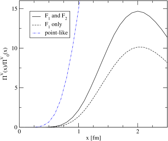
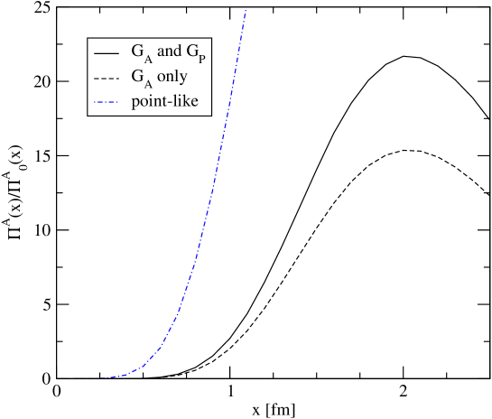
Figure 15: Nucleon pole contribution to the vector (upper panel) and axial-vector (lower panel) nucleon three-point function. The solid line shows the complete results, the dashed line is the contribution from the $F_{1}$ and $G_{A}$ form factors only, and the dash-dotted line corresponds to a point-like nucleon. We have used a nucleon coupling constant $\lambda=2.2\,{\rm fm}^{-3}$ as well as phenomenological values for the form factors and coupling constants.

In Fig. 15 we show the nucleon pole contribution to the vector and axial-vector three-point functions. We have used the phenomenological values of the isovector coupling constants

$$\begin{array}[]{rclcrcl}G_{E}(0)&=&1,&&G_{M}(0)&=&4.7,\\ G_{A}(0)&=&1.25,&&G_{P}(0)&=&\frac{4M^{2}}{m_{\pi}^{2}}g_{A}.\end{array}$$ (112)

We have parametrized $G_{E,V}$ and $G_{A}$ by dipole functions with $m_{V}=0.88$ GeV and $m_{A}=1.1$ GeV. The induced pseudoscalar form factor is parametrized as a pion propagator multiplied by a dipole form factor with dipole mass $m_{A}$.

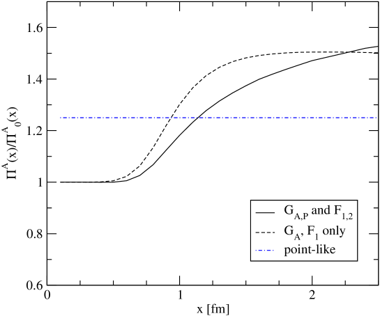
Figure 16: Ratio of the phenomenological parameterizations of the axial-vector and vector three-point functions. We have added a short distance continuum contribution to the nucleon pole terms. The curves are labeled as in the previous figure. Note that both the solid and the dashed line will approach $g_{A}=1.25$ as $x\to\infty$. Also note that the solid line is in very good agreement with the instanton calculation shown in Fig. 13.

We observe that at distances that are accessible in lattice or instanton simulations, $x\sim(1-2)$ fm, the typical momentum transfer is not small and the correlation function is substantially reduced as compared to the result for a point-like nucleon. We also observe that the $F_{2}$ and $G_{P}$ form factors make substantial contributions. Fig. 16 shows that the ratio of the axial-vector and vector correlation functions is nevertheless close to the value for a point-like nucleon, $g_{A}/g_{V}\simeq 1.25$. We observe that the ratio of point-to-point correlation functions approaches this value from above. This is related to the fact that the axial radius of the nucleon is smaller than the vector radius. As a consequence, the point-to-point correlation function at finite separation $\tau$ “sees” a larger fraction of the axial charge as compared to the vector charge.

Appendix B Instanton contribution to quark three-point functions

In this appendix we provide the results for the traces that appear in the single instanton contribution to the quark three-point function. Our starting point is the expression

$$(P^{con}_{A/VQQ})^{\mu\nu}=P_{NZNZ}^{\mu\nu}+c_{A/V}\left(P^{\mu\nu}_{ZMm}+P^{\mu\nu}_{mZM}\right),$$ (113)

see equ. (61). Due to the Dirac structure of the non-zero mode part of the propagator, the $NZNZ$ term is the same for both the vector and axial-vector correlation functions. It has 4 parts stemming from combinations of the two terms of non-zero mode propagator equ. 17

$$P_{NZNZ_{11}}^{\mu\nu} = \frac{2H(x,z,y)(x-z)^{\alpha}(z-y)^{\beta}}{\pi^{4}(x-z)^{4}(z-y)^{4}}S^{\nu\alpha\mu\beta}\left[1+\frac{\rho^{2}}{z^{2}}\left(\frac{x\cdot z}{x^{2}}+\frac{z\cdot y}{y^{2}}\right)+\frac{\rho^{4}x\cdot y}{x^{2}z^{2}y^{2}}\right],$$ (114)

$$P_{NZNZ_{12}}^{\mu\nu} = \frac{H(x,z,y)(x-z)^{\alpha}y^{\beta}}{2\pi^{4}(x-z)^{4}(z-y)^{2}z^{2}y^{2}}[(z^{\alpha_{0}}+\frac{\rho^{2}}{x^{2}}x^{\alpha_{0}})S^{\alpha_{0}\sigma\sigma_{0}\beta}\pm\frac{\rho^{2}}{x^{2}}x^{\alpha_{0}}\epsilon^{\alpha_{0}\sigma\sigma_{0}\beta}]$$ (115)

$$\times\left[\frac{\rho^{2}(z-y)^{\sigma_{0}}}{\rho^{2}+z^{2}}(S^{\nu\alpha\mu\sigma}\pm\epsilon^{\nu\alpha\mu\sigma})+\frac{\rho^{2}(z-y)^{\sigma}}{\rho^{2}+y^{2}}(S^{\nu\alpha\mu\sigma_{0}}\mp\epsilon^{\nu\alpha\mu\sigma_{0}})\right],$$

$$P_{NZNZ_{21}}^{\mu\nu} = \frac{H(x,z,y)(z-y)^{\alpha}x^{\beta}}{2\pi^{4}(x-z)^{2}(z-y)^{4}z^{2}x^{2}}[(z^{\alpha_{0}}+\frac{\rho^{2}}{y^{2}}y^{\alpha_{0}})S^{\beta\sigma\sigma_{0}\alpha_{0}}\pm\frac{\rho^{2}}{y^{2}}y^{\alpha_{0}}\epsilon^{\beta\sigma\sigma_{0}\alpha_{0}}]$$ (116)

$$\times\left[\frac{\rho^{2}(x-z)^{\sigma_{0}}}{\rho^{2}+x^{2}}(S^{\nu\sigma\mu\alpha}\pm\epsilon^{\nu\sigma\mu\alpha})+\frac{\rho^{2}(x-z)^{\sigma}}{\rho^{2}+z^{2}}(S^{\nu\sigma_{0}\mu\alpha}\mp\epsilon^{\nu\sigma_{0}\mu\alpha})\right],$$

$$P_{NZNZ_{22}}^{\mu\nu} = \frac{H(x,z,y)x^{\alpha_{0}}y^{\beta}}{4\pi^{4}(x-z)^{2}(z-y)^{2}z^{2}y^{2}x^{2}}\frac{\rho^{4}}{(\rho^{2}+z^{2})}\left[\frac{(x-z)^{\sigma}(z-y)^{\sigma_{1}}}{(\rho^{2}+x^{2})}(S^{\nu\alpha\mu\alpha_{1}}\pm\epsilon^{\nu\alpha\mu\alpha_{1}})\right.$$ (117)

$$+\left.\frac{(x-z)^{\alpha}(z-y)^{\alpha_{1}}}{(\rho^{2}+y^{2})}(S^{\nu\sigma\mu\sigma_{1}}\mp\epsilon^{\nu\sigma\mu\sigma_{1}})\right]T_{\pm}[\alpha_{0},\alpha,\sigma,\alpha_{1},\sigma_{1},\beta],$$

where

$$H(x,z,y)=\left\{\left(1+\frac{\rho^{2}}{z^{2}}\right)\sqrt{\left(1+\frac{\rho^{2}}{x^{2}}\right)\left(1+\frac{\rho^{2}}{y^{2}}\right)}\right\}^{-1}$$ (118)

and the Dirac trace $T_{\pm}$ is defined as

$$T_{\mp}[\mu,2,3,4,5,6] \equiv \left[\left(g^{\mu 2}S^{3456}-g^{\mu 3}S^{2456}+g^{\mu 4}S^{2356}-g^{\mu 5}S^{2346}+g^{\mu 6}S^{2345}\right)\right.$$ (119)

$$\mp\left.\left(g^{\mu 2}\epsilon^{3456}-g^{\mu 3}\epsilon^{2456}+g^{23}\epsilon^{\mu 456}+g^{45}\epsilon^{\mu 236}-g^{46}\epsilon^{\mu 235}+g^{56}\epsilon^{\mu 234}\right)\right],$$

where $2,3,\ldots$ is short for $\mu_{2},\mu_{3},\ldots$. The $S_{ZM}S_{m}$ term is easily seen to be

$$P^{\mu\nu}_{ZMm} = {\rm Tr}[-\Psi_{0}(x)\Psi_{0}^{+}(z)\gamma^{\mu}(-\Delta_{\pm}(z,y)\gamma_{\pm})\gamma^{\nu}]$$ (120)

$$= \frac{\varphi(x)\varphi(z)x^{\alpha_{0}}z^{\beta_{0}}}{8\pi^{2}(z-y)^{2}}\frac{1}{\sqrt{(1+\frac{\rho^{2}}{z^{2}})(1+\frac{\rho^{2}}{y^{2}})}}T_{\mp}[\alpha_{0},\sigma_{1},\sigma,\beta_{0},\mu,\nu]$$

$$\times\left[\delta^{\sigma_{1},\sigma}+\frac{\rho^{2}z^{\alpha}y^{\beta}}{z^{2}y^{2}}(S^{\sigma_{1}\sigma\alpha\beta}\pm\epsilon^{\sigma_{1}\sigma\alpha\beta})\right]$$

with $\varphi(x)=\rho/(\pi\sqrt{x}(x^{2}+\rho^{2})^{3/2})$. The $S_{m}S_{ZM}$ term is obtained similarly

$$P^{\mu\nu}_{mZM} = {\rm Tr}[(-\Delta_{\pm}(x,z)\gamma_{\pm})\gamma^{\mu}(-\Psi_{0}(z)\Psi_{0}^{+}(y))\gamma^{\nu}]$$ (121)

$$= \frac{\varphi(z)\varphi(y)z^{\alpha_{0}}y^{\beta_{0}}}{8\pi^{2}(x-z)^{2}}\frac{1}{\sqrt{(1+\frac{\rho^{2}}{x^{2}})(1+\frac{\rho^{2}}{z^{2}})}}T_{\mp}[\alpha_{0},\sigma_{1},\sigma,\beta_{0},\nu,\mu]\times$$

$$\times\left[\delta^{\sigma_{1},\sigma}+\frac{\rho^{2}x^{\alpha}z^{\beta}}{x^{2}z^{2}}(S^{\sigma_{1}\sigma\alpha\beta}\pm\epsilon^{\sigma_{1}\sigma\alpha\beta})\right].$$

For all the above formulas, we need to add instanton and anti-instanton contribution and integrate over the position of the instanton, which was suppressed above. As usual, for an instanton at position $z_{I}$ we have to shift $x,y,z$ according to $x\to(x-z_{I})$, etc.

References

- (1) J. Ashman et al. [European Muon Collaboration], Phys. Lett. B 206, 364 (1988).
- (2) B. W. Filippone and X. D. Ji, Adv. Nucl. Phys. 26, 1 (2001) [hep-ph/0101224].
- (3) A. E. Dorokhov, N. I. Kochelev and Y. A. Zubov, Int. J. Mod. Phys. A 8, 603 (1993).
- (4) S. D. Bass and A. W. Thomas, Prog. Part. Nucl. Phys. 33, 449 (1994) [hep-ph/9310306].
- (5) S. D. Bass, Acta Phys. Polon. B 34, 5893 (2003) [hep-ph/0311174].
- (6) G. Altarelli and G. G. Ross, Phys. Lett. B 212, 391 (1988).
- (7) R. L. Jaffe and A. Manohar, Nucl. Phys. B 337, 509 (1990).
- (8) M. A. Shifman, A. I. Vainshtein and V. I. Zakharov, Phys. Lett. B 78, 443 (1978).
- (9) A. Anselm, Phys. Lett. B 291, 455 (1992).
- (10) J. H. Kuhn and V. I. Zakharov, Phys. Lett. B 252, 615 (1990).
- (11) S. Narison, G. M. Shore and G. Veneziano, Nucl. Phys. B 433, 209 (1995) [hep-ph/9404277].
- (12) T. Schäfer and E. V. Shuryak, Rev. Mod. Phys. 70, 323 (1998) [hep-ph/9610451].
- (13) E. V. Shuryak and J. J. Verbaarschot, Phys. Rev. D 52, 295 (1995) [hep-lat/9409020].
- (14) T. Schäfer and E. V. Shuryak, preprint, hep-lat/0005025.
- (15) T. Schäfer, E. V. Shuryak and J. J. Verbaarschot, Nucl. Phys. B 412, 143 (1994) [hep-ph/9306220].
- (16) D. Diakonov, Prog. Part. Nucl. Phys. 51, 173 (2003) [hep-ph/0212026].
- (17) L. S. Brown, R. D. Carlitz, D. B. Creamer and C. K. Lee, Phys. Rev. D 17, 1583 (1978).
- (18) N. Andrei and D. J. Gross, Phys. Rev. D 18, 468 (1978).
- (19) P. Nason and M. Porrati, Nucl. Phys. B 421, 518 (1994) [hep-ph/9302211].
- (20) B. V. Geshkenbein and B. L. Ioffe, Nucl. Phys. B 166, 340 (1980).
- (21) A. E. Dorokhov and W. Broniowski, Eur. Phys. J. C 32, 79 (2003) [hep-ph/0305037].
- (22) M. S. Dubovikov and A. V. Smilga, Nucl. Phys. B 185, 109 (1981).
- (23) T. Schäfer, E. V. Shuryak and J. J. M. Verbaarschot, Phys. Rev. D 51, 1267 (1995) [hep-ph/9406210].
- (24) T. Schäfer and E. V. Shuryak, Phys. Rev. D 53, 6522 (1996) [hep-ph/9509337].
- (25) T. Schäfer and E. V. Shuryak, Phys. Rev. D 54, 1099 (1996) [hep-ph/9512384].
- (26) N. Isgur and H. B. Thacker, Phys. Rev. D 64, 094507 (2001) [hep-lat/0005006].
- (27) S. Weinberg, Phys. Rev. Lett. 67, 3473 (1991).
- (28) U. Vogl and W. Weise, Prog. Part. Nucl. Phys. 27, 195 (1991).
- (29) K. Steininger and W. Weise, Phys. Rev. D 48, 1433 (1993).
- (30) A. E. Dorokhov, preprint, hep-ph/0112332.
- (31) N. I. Kochelev, Phys. Rev. D 57, 5539 (1998) [hep-ph/9711226].
- (32) B. L. Ioffe, Nucl. Phys. B 188, 317 (1981) [Erratum-ibid. B 191, 591 (1981)].
- (33) R. Rapp, T. Schäfer, E. V. Shuryak and M. Velkovsky, Phys. Rev. Lett. 81, 53 (1998) [hep-ph/9711396].
- (34) D. B. Leinweber, Phys. Rev. D 51, 6383 (1995) [nucl-th/9406001].
- (35) M. Anselmino, E. Predazzi, S. Ekelin, S. Fredriksson and D. B. Lichtenberg, Rev. Mod. Phys. 65, 1199 (1993).
- (36) D. Dolgov, R. Brower, J. W. Negele and A. Pochinsky, Nucl. Phys. Proc. Suppl. 73, 300 (1999) [hep-lat/9809132].
- (37) S. J. Dong, J. F. Lagae and K. F. Liu, Phys. Rev. Lett. 75, 2096 (1995) [hep-ph/9502334].
- (38) S. Forte and E. V. Shuryak, Nucl. Phys. B 357, 153 (1991).
- (39) M. Hutter, preprint, hep-ph/9509402.
- (40) M. Kacir, M. Prakash and I. Zahed, Acta Phys. Polon. B 30, 287 (1999) [hep-ph/9602314].
- (41) D. Diakonov, M. V. Polyakov and C. Weiss, Nucl. Phys. B 461, 539 (1996) [hep-ph/9510232].
- (42) D. Diakonov, V. Y. Petrov and P. V. Pobylitsa, Nucl. Phys. B 306, 809 (1988).
- (43) S. J. Brodsky, J. R. Ellis and M. Karliner, Phys. Lett. B 206, 309 (1988).
- (44) A. Blotz, M. V. Polyakov and K. Goeke, Phys. Lett. B 302, 151 (1993).
- (45) P. Faccioli, preprint, hep-ph/0312019.
- (46) L. Maiani and M. Testa, Phys. Lett. B 245, 585 (1990).