hep-ph/0401160
MCTP-04-03

Saclay t04/009

Oblique Corrections from Higgsless Models in Warped Space

Giacomo Cacciapaglia^a, Csaba Csáki^a, Christophe Grojean^b,c,
and John Terning^d

^a Institute for High Energy Phenomenology
Newman Laboratory of Elementary Particle Physics
Cornell University, Ithaca, NY 14853, USA

^b Service de Physique Théorique, CEA Saclay, F91191 Gif–sur–Yvette, France

^c Michigan Center for Theoretical Physics, Ann Arbor, MI 48109, USA
^d Theory Division T-8, Los Alamos National Laboratory, Los Alamos, NM 87545, USA

cacciapa@lepp.cornell.edu, csaki@lepp.cornell.edu, grojean@spht.saclay.cea.fr, terning@lanl.gov

We calculate the tree-level oblique corrections to electroweak precision observables generated in higgless models of electroweak symmetry breaking with a 5D SU(2)${}_{L}\times$SU(2)_R $\times$U(1)_B-L gauge group on a warped background. In the absence of brane induced kinetic terms (and equal left and right gauge couplings) we find the $S$ parameter to be $\sim 1.15$, while $T\sim U\sim 0$, as in technicolor theories. Planck brane induced kinetic terms and unequal left-right couplings can lower $S$, however for sufficiently low values of $S$ tree-level unitarity will be lost. A kinetic term localized on the TeV brane for SU(2)_D will generically increase $S$, however an induced kinetic term for U(1)_B-L on the TeV brane will lower $S$. With an appropriate choice of the value of this induced kinetic term $S\sim 0$ can be achieved. In this case the mass of the lowest Z^′ mode will be lowered to about $300$ GeV.

1 Introduction

Finding the correct mechanism for electroweak symmetry breaking is perhaps the most important problem facing particle physics. The simplest possibility is via a standard model (SM) Higgs field, however the mass of such a Higgs is unstable to radiative corrections. The usual ways to overcome this problem is either to assume that the Higgs mass is stabilized by supersymmetry, or that electroweak symmetry is broken dynamically by some interaction becoming strong around the TeV scale. Extra dimensions may also offer possible ways of stabilizing the Higgs mass against radiative corrections, either by lowering the scale of gravity in large extra dimensions [1], by localizing gravity away from the SM fields in the RS model [2], or by the Higgs secretly being the scalar component $A_{5}$ of an extra dimensional gauge field [3] (the 4D implementation of this last approach leads to the recently proposed [4] little Higgs models). However, extra dimensions could not only offer new ways to stabilize the Higgs mass, but also a completely new mechanism to break the symmetry itself without the existence of a Higgs: boundary conditions at the endpoints of a finite extra dimension could break a gauge symmetry, in which case unitarity of the scattering amplitudes of massive gauge bosons (GB’s) is not cured by the exchange of the physical Higgs scalar, but rather by the exchange of a tower of massive KK gauge bosons [5] (see also [6]). A toy model with massive W and Z bosons of this sort was presented in [5]. In order to find a realistic higgsless model of electroweak symmetry breaking one needs to overcome several problems. The first is the question of how to ensure that the boundary conditions (BC’s) give the right $M_{W}/M_{Z}$ mass ratio. The correct tree-level prediction is usually ensured by a custodial SU(2) global symmetry in the sector that breaks the electroweak symmetry. The way to implement custodial SU(2) in an extra dimensional theory is by putting SU(2)${}_{L}\times$SU(2)_R gauge bosons in an anti-de Sitter (AdS) background [7]. The reason behind this lies in the holographic interpretation of an AdS bulk: it is supposed to correspond to a four dimensional conformal field theory (CFT) which has a global symmetry dictated by the gauge symmetries in the bulk. Those symmetries broken on the Planck brane (the UV brane) will be interpreted as global symmetries, while those unbroken will remain as weakly gauged global symmetries of the CFT all the way down to the TeV scale. Based on this insight, [8] considered a 5D gauge theory on an AdS₅ background with SU(2)${}_{L}\times$SU(2)${}_{R}\times$U(1)_B-L gauge bosons in the bulk. SU(2)${}_{R}\times$U(1)_B-L is broken to U(1)_Y on the Planck brane, leaving the broken generators as global symmetries (and thus ensuring the custodial SU(2) symmetry necessary for recovering the GB mass ratios). On the TeV brane SU(2)${}_{L}\times$SU(2)_R is broken to SU(2)_D thereby breaking electroweak symmetry. This theory could be considered as the AdS/CFT dual of walking technicolor [10]: the CFT runs slowly until energies where the TeV brane appears and electroweak symmetry is broken. It was shown in [8] (and in [11] for the same model with an enlarged parameter space) that the leading SM predictions are recovered in this setup: one gets the correct W/Z mass ratio and coupling to fermions localized close to the Planck brane. The KK modes of the W and Z are heavy enough to have escaped direct detection, but just light enough to unitarize the scattering amplitudes. For the simplest choice of parameters the first of these KK modes would appear at around 1.2 TeV.

Two important issues have to be addressed to make the model completely realistic: how to generate fermion masses in the absence of a Higgs scalar, and how large the corrections to electroweak precision observables would be. In [12] (and also in [8, 9, 11]) it has been shown that it is possible to obtain a realistic fermion mass spectrum in this model: the unbroken gauge group on the TeV brane is non-chiral, so an explicit mass term can be added there. In order to lift the SU(2)_D degeneracy, mixing with Planck brane localized fermions can be added (which is equivalent to adding different brane localized kinetic terms for the right handed up vs. down type quarks, or neutrinos vs. charged leptons). The issue of electroweak precision observables in higgsless theories was first discussed in [9], where it was argued that in generic higgsless models there will be an $S$ parameter of order one generated (analogously to technicolor theories). In this paper we investigate the tree-level oblique corrections to electroweak precision observables in the warped higgsless model in terms of the input parameters of the theory. We find, that in the absence of brane induced kinetic terms (and equal left and right couplings) $S\sim 1.15,T\sim U\sim 0$. Unequal L,R couplings or Planck brane induced kinetic terms can lower $S$ to acceptable values only at the price of losing tree-level unitarity (thus entering a strong coupling regime). TeV brane induced SU(2) kinetic terms generically raise the value of $S$, however a TeV brane induced kinetic term for the U(1)_B-L gauge group lowers $S$. By choosing an appropriate value for this coupling one can obtain $S\sim 0$ (and a moderately negative $T$). In this case the mass of the lightest Z^′ KK mode is lowered to about 300 GeV.

Note however, that while this analysis does give a large fraction of the corrections to electroweak precision observables, one should not directly compare the values of $S,T,U$ obtained here to the usually quoted experimental values. The reason is that the experimentally allowed values of $S,T,U$ are usually extracted from the data assuming the existence of a SM Higgs with a certain mass (usually 115 GeV). Here however there is no Higgs particle, so its contribution should be subtracted from the analysis. This procedure is however complicated by the fact that only the sum of the gauge plus Higgs sector gives a finite and gauge invariant contribution to the oblique parameters, so the right approach would be to replace this sum with the 1-loop contribution of the full KK tower of the W and Z. In addition, depending on the actual fermion mass model, there can be large non-oblique corrections to the interactions of the third generation, in particular to the $Zb\bar{b}$ vertex. These issues are left for further investigation. Further interesting questions regarding higgsless models have been discussed in [13, 14, 15]: non-perturbative arguments for unitarity of models with BC breaking of gauge symmetries have been presented in [13, 14], while deconstruction of the higgsless models was considered in [15] (see also [5]).

This paper is organized as follows: in Section 2 we discuss the setup and the expansion of the wave functions to sub-leading order in $1/\log(R^{\prime}/R)\sim 1/30$. In section 3 we present the calculation of the oblique corrections for the simplest point on the parameter space. In Section 4 we extend this calculation to asymmetric gauge couplings, and more importantly including brane induced kinetic terms. We show how $S$ can be lowered using the U(1)_B-L induced kinetic term on the TeV brane, and briefly discuss the properties of the lightest Z^′ mode for the case with small $S$. We conclude in Section 5.

While this paper was in preparation, two related studies [16, 17] of the oblique corrections to electroweak precision observables in higgsless models appeared, which have a considerable overlap with our work.

2 The model

We will consider the model discussed in [8]: an SU(2)${}_{L}\times$SU(2)${}_{R}\times$U(1)_B-L gauge theory on a fixed AdS₅ background. We will use the conformally flat metric

$$ds^{2}=\left(\frac{R}{z}\right)^{2}\Big{(}\eta_{\mu\nu}dx^{\mu}dx^{\nu}-dz^{2}\Big{)}$$ (2.1)

where $z$ is on the interval $[R,R^{\prime}]$. The bulk Lagrangian for the gauge fields (after decomposing the 5D gauge boson into a 4D gauge boson $A_{\mu}^{a}$ and a 4D scalar $A_{5}^{a}$ in the adjoint representation, and adding the appropriate gauge fixing terms in R_ξ gauge) are of the form

$$\mathcal{S}=\int d^{4}x\,\int_{R}^{R^{\prime}}dz\,\frac{R}{z}\,\left(-\frac{1}{4}F_{\mu\nu}^{a}F^{a\mu\nu}-\frac{1}{2}F_{5\nu}^{a}F^{a5\nu}-\frac{1}{2\xi}(\partial_{\mu}A^{a\mu}-\xi\partial_{5}A_{5}^{a})^{2}\right),$$ (2.2)

where $M=0,1,2,3,5$ denotes 5D Lorentz indices while $\mu=0,1,2,3$ are used to denote usual 4D Lorentz indices. $F^{a}_{MN}=\partial_{M}A_{N}^{a}-\partial_{N}A_{M}^{a}+g_{5}f^{abc}\,A^{b}_{M}A^{c}_{N}$, and the $f^{abc}$’s are the structure constants of the gauge group, and we have $F^{a}_{MN}=(W^{L,a}_{MN},W^{R,a}_{MN},B_{MN})$ for the SU(2)_L, SU(2)_R, U(1)_B-L gauge groups. We will denote the 5D gauge couplings of these groups by $g_{5L},g_{5R}$ and $\tilde{g}_{5}$. Taking $\xi\to\infty$ will result in the unitary gauge, where all the KK modes of the scalars fields $A^{a}_{5}$ are unphysical (they become the longitudinal modes of the 4D gauge bosons), except if there is a zero mode for the $A_{5}$’s. A zero mode in $A_{5}$ would correspond to a Goldstone boson in the holographic interpretation. Such Goldstone modes exist if some of the bulk gauge symmetries are broken both on the Planck brane and the TeV brane. In the model considered below this will not be the case, and so will assume that every $A_{5}^{a}$ mode is massive, and thus that all the $A_{5}$’s are eliminated in the unitary gauge.

We denote by $A^{R\,a}_{M}$, $A^{L\,a}_{M}$ and $B_{M}$ the gauge bosons of $SU(2)_{R}$, $SU(2)_{L}$ and $U(1)_{B-L}$ respectively. For simplicity we will first assume $g_{5L}=g_{5R}=g_{5}$ (later on we will relax this assumption). We impose the following BC’s:

$${\rm at}\ z=R^{\prime}: \left\{\begin{array}[]{l}\partial_{z}(A^{L\,a}_{\mu}+A^{R\,a}_{\mu})=0,\ A^{L\,a}_{\mu}-A^{R\,a}_{\mu}=0,\ \partial_{z}B_{\mu}=0,\\ \vrule height=15.0pt,depth=5.0pt,width=0.0pt(A^{L\,a}_{5}+A^{R\,a}_{5})=0,\ \partial_{z}(A^{L\,a}_{5}-A^{R\,a}_{5})=0,\ B_{5}=0.\end{array}\right.$$ (2.5)

$${\rm at}\ z=R: \left\{\begin{array}[]{l}\partial_{5}A^{L\,a}_{\mu}=0,\ A^{R\,1,2}_{\mu}=0,\\ \vrule height=15.0pt,depth=5.0pt,width=0.0pt\partial_{z}(g_{5}B_{\mu}+\tilde{g}_{5}A^{R\,3}_{\mu})=0,\ \tilde{g}_{5}B_{\mu}-g_{5}A^{R\,3}_{\mu}=0,\\ \vrule height=15.0pt,depth=5.0pt,width=0.0ptA^{L\,a}_{5}=0,\ A^{R\,a}_{5}=0,\ B_{5}=0.\end{array}\right.$$ (2.9)

The KK expansion is given by

$$B_{\mu}(x,z) = \frac{1}{\tilde{g}_{5}}\,a_{0}\gamma_{\mu}(x)+\sum_{k=1}^{\infty}\psi^{(B)}_{k}(z)\,Z^{(k)}_{\mu}(x)\,,$$ (2.10)

$$A^{L\,3}_{\mu}(x,z) = \frac{1}{g_{5}}\,a_{0}\gamma_{\mu}(x)+\sum_{k=1}^{\infty}\psi^{(L3)}_{k}(z)\,Z^{(k)}_{\mu}(x)\,,$$ (2.11)

$$A^{R\,3}_{\mu}(x,z) = \frac{1}{g_{5}}\,a_{0}\gamma_{\mu}(x)+\sum_{k=1}^{\infty}\psi^{(R3)}_{k}(z)\,Z^{(k)}_{\mu}(x)\,,$$ (2.12)

$$A^{L\,\pm}_{\mu}(x,z) = \sum_{k=1}^{\infty}\psi^{(L\pm)}_{k}(z)\,W^{(k)\,\pm}_{\mu}(x)\,,$$ (2.13)

$$A^{R\,\pm}_{\mu}(x,z) = \sum_{k=1}^{\infty}\psi^{(R\pm)}_{k}(z)\,W^{(k)\,\pm}_{\mu}(x)\,.$$ (2.14)

The Euclidean bulk equation of motion satisfied by spin-1 fields in AdS space is

$$(\partial_{z}^{2}-\frac{1}{z}\partial_{z}+q^{2})\psi(z)=0,$$ (2.15)

where the solutions in the bulk are assumed to be of the form $A^{a}_{\mu}(q)e^{-iqx}\psi(z)$. The KK mode expansion is given by the solutions to this equation which are of the form

$$\psi^{(A)}_{k}(z)=z\left(a^{(A)}_{k}J_{1}(q_{k}z)+b^{(A)}_{k}Y_{1}(q_{k}z)\right)~{},$$ (2.16)

where $A$ labels the corresponding gauge boson.

Next we want to do an expansion in $1/\log(R^{\prime}/R)$ for the wave functions of the gauge bosons. When $R^{\prime}\to\infty$, the TeV brane is sent to infinity, and thus there is no electroweak symmetry breaking. So in this limit $M_{W},M_{Z}\to 0$, and the wave functions will be exactly flat. For finite $R^{\prime}$, $M_{W}^{2},M_{Z}^{2}\propto 1/\log(R^{\prime}/R)$ [8]. This means that the argument of the gauge boson wave function $Mz$ is at most of order $1/\log(R^{\prime}/R)$, thus an expansion in small arguments for the Bessel functions is justified and all quantities related to the light gauge bosons should have a well-defined expansion in $1/\log(R^{\prime}/R)$. In [8] we have shown that the leading terms $\sim 1/\log(R^{\prime}/R)$ in this log expansion exactly reproduce the SM mass relations and the SM couplings. The $1/\log^{2}(R^{\prime}/R)$ will then correspond to the leading corrections to the electroweak precision observables. In the rest of this section we will find the corrections to the gauge boson wave functions to order $1/\log^{2}(R^{\prime}/R)$, which we will then use in the next section to get the oblique correction parameters $S,T,U$ to electroweak precision observables.

From the expansion for small arguments of the Bessel functions appearing in (2.16), the wavefunction of a mode with mass $M\ll 1/R^{\prime}$ can be written as (analogously to the expansions in [8, 18]):

$$\psi^{(A)}(z) \approx c_{0}^{(A)}+M_{A}^{2}z^{2}\left(c_{1}^{(A)}-\frac{c_{0}^{(A)}}{2}\log(z/R)\right)$$ (2.17)

$$+M_{A}^{4}z^{4}\left(-\frac{c_{1}^{(A)}}{8}-\frac{3c_{0}^{(A)}}{64}+\frac{c_{0}^{(A)}}{16}\log(z/R)\right)+{\cal O}(M_{A}^{6}z^{6}),$$

with $c_{1}^{(A)}$ at most ${\cal O}(c_{0}^{(A)}\log(R^{\prime}/R))$, and $(MR^{\prime})^{2}\sim{\cal O}(1/\log(R^{\prime}/R))$. The integrals of these wave functions that will be relevant for electroweak precision observables are given by (suppressing the index $A$):

$$\int_{R}^{R^{\prime}}\,\frac{dz}{z}\psi(z)^{2} \approx c_{0}^{2}\log\left(\frac{R^{\prime}}{R}\right)+M^{2}R^{\prime 2}\left(c_{0}c_{1}-\frac{1}{2}c_{0}^{2}\log{\textstyle\frac{R^{\prime}}{R}}\right)$$

$$+M^{4}R^{\prime 4}\left(\frac{c_{0}^{2}\left(\log{\textstyle\frac{R^{\prime}}{R}}\right)^{2}}{16}-\frac{c_{0}c_{1}\log{\textstyle\frac{R^{\prime}}{R}}}{4}+\frac{c_{1}^{2}}{4}\right)+{\cal O}\left(\frac{1}{\log{\textstyle\frac{R^{\prime}}{R}}}\right)$$

$$\int_{R}^{R^{\prime}}\,\frac{dz}{z}\left[\partial_{z}\psi(z)\right]^{2} \approx \left(\frac{M^{4}R^{\prime 2}}{2}-\frac{M^{6}R^{\prime 4}}{8}\right)\left(c_{0}^{2}\left(\log{\textstyle\frac{R^{\prime}}{R}}\right)^{2}-4c_{0}c_{1}\log{\textstyle\frac{R^{\prime}}{R}}+4c_{1}^{2}\right)$$

$$+{\cal O}\left(\frac{1}{\left(\log{\textstyle\frac{R^{\prime}}{R}}\right)^{2}}\right)$$

The boundary conditions on the bulk gauge fields give the following results for the leading and next-to-leading log terms in the wavefunction for the lightest charged gauge bosons

$$c_{0}^{(L\pm)} \equiv c_{\pm}~{},\ \ c_{0}^{(R\pm)}={\cal O}\left(c_{\pm}\frac{R^{2}}{R^{\prime 2}}\right)\approx 0~{},$$ (2.20)

$$c_{1}^{(L\pm)} \approx \frac{c_{\pm}}{4}~{},\ \ c_{1}^{(R\pm)}\approx\frac{c_{\pm}}{2}\log\left(\frac{R^{\prime}}{R}\right)+{\cal O}\left(\frac{c_{\pm}}{\log\left(\frac{R^{\prime}}{R}\right)}\right)~{},$$ (2.21)

while for the neutral gauge bosons we find in the same approximation

$$c_{0}^{(L3)}\equiv\,c~{},\ \ c_{0}^{(R3)}\approx-c\,\frac{\tilde{g}_{5}^{2}}{g_{5}^{2}+\tilde{g}_{5}^{2}}~{},\ \ c_{0}^{(B)}\approx-c\,\frac{g_{5}\,\tilde{g}_{5}}{g_{5}^{2}+\tilde{g}_{5}^{2}}~{}.$$ (2.22)

To leading log order we also have:

$$c_{1}^{(L3)} \approx \,\frac{c}{4}~{},$$ (2.23)

$$c_{1}^{(R3)} \approx \frac{c}{2}\,\frac{g_{5}^{2}}{g_{5}^{2}+\tilde{g}_{5}^{2}}\log\frac{R^{\prime}}{R}-\frac{c}{4}\,\frac{\tilde{g}_{5}^{2}}{g_{5}^{2}+\tilde{g}_{5}^{2}}+\ldots~{},$$ (2.24)

$$c_{1}^{(B)} \approx -\frac{c}{2}\,\frac{g_{5}\,\tilde{g}_{5}}{g_{5}^{2}+\tilde{g}_{5}^{2}}\log\frac{R^{\prime}}{R}-\frac{c}{4}\,\frac{g_{5}\,\tilde{g}_{5}}{g_{5}^{2}+\tilde{g}_{5}^{2}}+\ldots~{}.$$ (2.25)

To leading order in $1/R$ and to next-to-leading order in $1/\log\left(R^{\prime}/R\right)$, the lightest solution for this equation for the mass of the $W^{\pm}$’s is

$$M_{W}^{2}=\frac{1}{R^{\prime 2}\log\left(\frac{R^{\prime}}{R}\right)}\left(1+\frac{3}{8\log\frac{R^{\prime}}{R}}\right)\,,$$ (2.26)

while the lowest mass of the $Z$ tower is approximately given by

$$M_{Z}^{2}=\frac{g_{5}^{2}+2\tilde{g}_{5}^{2}}{g_{5}^{2}+\tilde{g}_{5}^{2}}\frac{1}{R^{\prime 2}\log\left(\frac{R^{\prime}}{R}\right)}\left(1+\frac{3}{8\log\frac{R^{\prime}}{R}}\frac{g_{5}^{2}+2\tilde{g}_{5}^{2}}{g_{5}^{2}+\tilde{g}_{5}^{2}}\right)\,.$$ (2.27)

3 Oblique Corrections to Precision Electroweak Observables

To calculate precision electroweak corrections we first need to choose a “renormalization convention.” Our aim is to find a scheme in which all corrections will be oblique (that is the effective 4D Lagrangian describing the coupled gauge boson-fermion system only gets corrections in the gauge boson sector, but not the fermion sector). With bulk gauge kinetic terms normalized by $1/g_{5}^{2}$ a very simple convention is to set the gauge boson wavefunction to be one at the location of the fermion [18]. Here we have chosen canonical normalization. What we need to require is that the couplings of Planck brane localized fermions give exactly the leading order relations for the couplings. This definition will make the corrections oblique. The couplings of an SU(2)_L doublet fermion to the vector gauge bosons are read off from the bulk covariant derivative evaluated at the location of the fermion, i.e., at the Planck brane:

$$\left(g_{5}T_{3}A^{L3}_{\mu}+g_{5}T_{\pm}A^{L\mp}_{\mu}+\frac{Y}{2}\tilde{g}_{5}B_{\mu}\right)_{|z=R}=\\ a_{0}Q\gamma_{\mu}+g_{5}\psi_{1}^{L\mp}(R)T_{\pm}W^{\mp}_{\mu}+g_{5}\psi_{1}^{(L3)}(R)\left(T_{3}+\frac{\tilde{g}_{5}\psi_{1}^{(B)}(R)}{g_{5}\psi_{1}^{(L3)}(R)}\frac{Y}{2}\right)Z_{\mu}~{},$$ (3.1)

where we have used the KK expansion (2.10)-(2.14) as well as the relation $\tilde{g}_{5}B_{\mu}=g_{5}A_{\mu}^{L3}$ for the photon wavefunction. $Y$ is the SM hypercharge of the fermion, $Q=Y/2+T_{3L}$ its electric charge. Using the BC $\tilde{g}_{5}B_{\mu}=g_{5}A_{\mu}^{R3}$ on the Planck brane, an identical expression also holds for the SU(2)_L singlet fermions that are embedded into SU(2)_R doublet representations (see Ref. [12] for details).

We now have to compare these couplings with the SM ones. The first point to note is that in this formula, the only quantity completely fixed by the BC’s, and then independent on the overall normalizations of the W and the Z, is the ratio of the $Z$ couplings to the $T_{3}$ and $Y$ component of the fermion. Thus, in order to recover the SM couplings for the fermions and ensure that besides the oblique corrections there are no other corrections we will have to impose that the one ratio independent of the normalizations reproduces the SM result:

$$\frac{g^{\prime 2}}{g^{2}}=-\frac{\tilde{g}_{5}\psi_{1}^{(B)}(R)}{g_{5}\psi_{1}^{(L3)}(R)}~{}.$$ (3.2)

Moreover, due to the unbroken U(1)_em it is always possible to canonically normalize the photon kinetic term in the effective 4D Lagrangian, thus we choose

$$Z_{\gamma} = \int_{R}^{R^{\prime}}[\Psi^{\gamma}]^{2}\left(\frac{R}{z}\right)dz=\int_{R}^{R^{\prime}}([a_{0}/{\tilde{g}_{5}}]^{2}+2[a_{0}/g_{5}]^{2})\left(\frac{R}{z}\right)dz=1~{}.$$ (3.3)

Since the photon wave function is flat it is easy to find its coupling to the Planck brane fermions and thus define the electric charge ($1/e^{2}=1/g^{2}+1/g^{\prime 2}$) as:

$$\frac{1}{e^{2}}=\frac{1}{a_{0}^{2}}=\left(\frac{1}{\tilde{g}_{5}^{2}}+\frac{2}{g_{5}^{2}}\right)R\log R^{\prime}/R~{}.$$ (3.4)

The two equations (3.2) and (3.4) completely define the 4 dimensional SM gauge couplings in terms of the 5D parameters. At the leading order in the log expansion, we recover the relations obtained in [8]:

$$g^{2} = \frac{g_{5}^{2}}{R\log(R^{\prime}/R)},$$ (3.5)

$$e^{2} = \frac{g_{5}^{2}\tilde{g}_{5}^{2}}{(g_{5}^{2}+2\tilde{g}_{5}^{2})R\log(R^{\prime}/R)},$$ (3.6)

$$g^{\prime 2} = \frac{g_{5}^{2}\tilde{g}_{5}^{2}}{(g_{5}^{2}+\tilde{g}_{5}^{2})R\log(R^{\prime}/R)},$$ (3.7)

$$\sin\theta_{W} = \frac{\tilde{g}_{5}}{\sqrt{g_{5}^{2}+2\tilde{g}_{5}^{2}}}.$$ (3.8)

Note, however, that Eqs. (3.2) and (3.4) will remain the correct definitions of the couplings even to higher orders in the log expansion. Furthermore, together with Eq. (3.1), they determine the remaining normalization factors that are set by requiring the correct couplings for the $W$ and $Z$, namely:

$$g_{5}\psi_{1}^{(L\pm)}(R) = g~{},$$ (3.9)

$$g_{5}\psi_{1}^{(L3)}(R) = g\cos\theta_{W}~{}.$$ (3.10)

Thus, at the leading order, the normalization coefficients in (2.20)-(2.25) are:

$$c_{\pm} = \frac{1}{\sqrt{R\log(R^{\prime}/R)}},$$ (3.11)

$$c = \sqrt{\frac{g_{5}^{2}+\tilde{g}_{5}^{2}}{g_{5}^{2}+2\tilde{g}_{5}^{2}}}\frac{1}{\sqrt{R\log(R^{\prime}/R)}},$$ (3.12)

$$a_{0} = \frac{g_{5}\tilde{g}_{5}}{\sqrt{(g_{5}^{2}+2\tilde{g}_{5}^{2})R\log(R^{\prime}/R)}}.$$ (3.13)

All the oblique corrections are now contained in the wavefunction and mass renormalizations of the gauge bosons. The wave function renormalizations are given by

$$Z_{W} = \int_{R}^{R^{\prime}}[\Psi^{W}]^{2}\left(\frac{R}{z}\right)dz=\int_{R}^{R^{\prime}}([\Psi^{L+}]^{2}+[\Psi^{R+}]^{2})\left(\frac{R}{z}\right)dz,$$ (3.14)

$$Z_{Z} = \int_{R}^{R^{\prime}}[\Psi^{Z}]^{2}\left(\frac{R}{z}\right)dz=\int_{R}^{R^{\prime}}([\Psi^{L3}]^{2}+[\Psi^{R3}]^{2}+[\Psi^{B}]^{2})\left(\frac{R}{z}\right)dz.$$ (3.15)

It is convenient to define equivalent vacuum polarization functions for these wavefunction renormalizations. Since we have already seen that $Z_{\gamma}=1$, the corresponding vacuum polarization

$$\Pi_{QQ}^{\prime}=\frac{d}{dp^{2}}\Pi_{QQ}(p^{2})|_{p^{2}=0}$$ (3.16)

vanishes. Also, since we are doing a tree-level calculation, there is no $Z-\gamma$ mixing and thus $\Pi_{3Q}^{\prime}$ also vanishes. We are left with the simple relations:

$$Z_{W}=1-g^{2}\Pi_{11}^{\prime}~{},\ \ \ \ \ \ \ \ Z_{Z}=1-(g^{2}+g^{\prime\,2})\Pi_{33}^{\prime}~{}.$$ (3.17)

With these definitions we find

$$\Pi_{11}^{\prime}=\Pi_{33}^{\prime}=\frac{3}{8}\frac{1}{g^{2}\log\frac{R^{\prime}}{R}}~{}.$$ (3.18)

Similarly we can calculate the vacuum polarizations at zero momentum, corresponding to the mass renormalizations of the gauge bosons:

$$g^{2}\Pi_{11}(0) = \int_{R}^{R^{\prime}}([\partial_{z}\Psi^{L+}]^{2}+[\partial_{z}\Psi^{R+}]^{2})\left(\frac{R}{z}\right)dz,$$ (3.19)

$$(g^{2}+g^{\prime\,2})\Pi_{33}(0) = \int_{R}^{R^{\prime}}([\partial_{z}\Psi^{L3}]^{2}+[\partial_{z}\Psi^{R3}]^{2}+[\partial_{z}\Psi^{B}]^{2})\left(\frac{R}{z}\right)dz.$$ (3.20)

Note that $\Pi_{QQ}(0)$ vanishes because the photon is exactly massless. We find

$$\Pi_{11}(0)=\Pi_{33}(0)=\frac{1}{g^{2}R^{\prime 2}\log\frac{R^{\prime}}{R}}+\mathcal{O}\left(\frac{1}{\left(\log\frac{R^{\prime}}{R}\right)^{3}}\right)~{}.$$ (3.21)

As a consistency check we can also show that the correction to the W mass is correctly reproduced by the $\Pi^{\prime}s$:

$$M_{W}^{2}=g^{2}\Pi_{11}(0)(1+g^{2}\Pi_{11}^{\prime})=\frac{1}{R^{\prime 2}\log\frac{R^{\prime}}{R}}\left(1+\frac{3}{8\log\frac{R^{\prime}}{R}}\right)~{}.$$ (3.22)

Note, that in the absence of a Higgs VEV the leading contribution to the W mass itself comes from $\Pi_{11}(0)$, as happens in technicolor models as well.

The oblique correction parameters in terms of these vacuum polarization functions are defined as [19]:

$$S \equiv 16\pi\,\big{(}\Pi_{33}^{\prime}-\Pi_{3Q}^{\prime}\big{)},$$

$$T \equiv \frac{4\pi}{\sin^{2}\theta_{W}\cos^{2}\theta_{W}\,M_{Z}^{2}}\,\big{(}\Pi_{11}(0)-\Pi_{33}(0)\big{)},$$ (3.23)

$$U \equiv 16\pi\,\big{(}\Pi_{11}^{\prime}-\Pi_{33}^{\prime}\big{)}.$$

For fermions localized on the Planck brane we find:

$$S \approx \frac{6\pi}{g^{2}\log\frac{R^{\prime}}{R}}\approx 1.15,$$ (3.24)

$$T = 0,$$ (3.25)

$$U = 0~{}.$$ (3.26)

Thus just as in technicolor models we find that there is a large positive contribution to the $S$ parameter. In technicolor language this corresponds to the effects of the CFT. The vanishing of $T$ is ensured by the custodial SU(2) symmetry close to the TeV brane. These results are in agreement with the expectations presented in [9].

The experimental values of $S,T,U$ are [20]

$$S = -0.03\pm 0.11$$ (3.27)

$$T = -0.02\pm 0.13$$ (3.28)

$$U = 0.24\pm 0.13~{}.$$ (3.29)

Clearly, with these central values $S$ is too large by a factor of 5-6 in order to be consistent with the electroweak precision observables. However, the above experimental values have been obtained assuming the existence of a SM Higgs with mass of 115 GeV. In order to correctly compare this model with the experimental result, the contribution of the Higgs would have to be subtracted. This is however harder than it may sound at first, since the Higgs contribution is finite and gauge invariant at one loop only together with the contribution of the W,Z gauge bosons. In this model what will likely happen is that the Higgs+W,Z contributions have to be replaced by the full 1-loop contribution of the entire W,Z KK towers in order to obtain a gauge invariant answer. This would be very interesting to do, here however we will not follow this route, but rather try to see if the introduction of more parameters could reduce the size of the correction to $S$.

4 Asymmetric gauge couplings and brane localized kinetic terms.

In this section, we analyse the more general case where the bulk gauge couplings of the $SU(2)_{L}$ and $SU(2)_{R}$ are different, $g_{5R}$ and $g_{5L}$, and brane kinetic terms allowed by the gauge symmetries of the theory are added. Some of these parameters have already been considered in [11], where it was shown that turning on these parameters does not change the leading order predictions for the SM masses and couplings. The AdS/CFT interpretation of different left-right bulk gauge couplings is that the CFT does not have a left-right interchange symmetry, or in other words is a chiral gauge theory, and so in our context such models are analogous to chiral technicolor [21]. On the Planck brane, the only allowed kinetic terms involve the locally unbroken SM group SU(2)${}_{L}\times$U(1)_Y. On the other hand, on the TeV brane the unbroken groups are the $U(1)_{B-L}$ and $SU(2)_{D}$, so that their effect is to mix the SM gauge bosons. In the case of $SU(2)_{D}$ it is clear that there is a direct contribution to the $S$ parameter, not suppressed by a log. In both cases there will be corrections to $S$, $T$, and $U$ even when the wavefunction is only kept to leading log order. For this reason we will deal with the TeV brane induced terms separately.

4.1 Planck brane kinetic terms.

The bulk Lagrangian is as in (2.2), except now $g_{5L}\neq g_{5R}$. The localized Lagrangian on the Planck brane is:

$$\mathcal{L}_{Pl}=-\left[\frac{r}{4}{W^{L}_{\mu\nu}}^{2}+\frac{r^{\prime}}{4}\frac{1}{g_{5R}^{2}+\tilde{g}_{5}^{2}}(g_{5R}B_{\mu\nu}+\tilde{g}_{5}W^{R3}_{\mu\nu})^{2}\right]\delta(z-R)~{},$$ (4.1)

where the parameters $r$ and $r^{\prime}$ have dimension of length. The presence of the localized kinetic terms modifies the BC’s for the gauge bosons which now read:

$${\rm at}\ z=R^{\prime}: \left\{\begin{array}[]{l}\partial_{z}(g_{5R}A^{L\,a}_{\mu}+g_{5L}A^{R\,a}_{\mu})=0,\ g_{5L}A^{L\,a}_{\mu}-g_{5R}A^{R\,a}_{\mu}=0,\ \partial_{z}B_{\mu}=0,\\ \vrule height=15.0pt,depth=5.0pt,width=0.0pt(g_{5R}A^{L\,a}_{5}+g_{5L}A^{R\,a}_{5})=0,\ \partial_{z}(g_{5L}A^{L\,a}_{5}-g_{5R}A^{R\,a}_{5})=0,\ B_{5}=0.\end{array}\right.$$ (4.4)

$${\rm at}\ z=R: \left\{\begin{array}[]{l}\partial_{5}A^{L\,a}_{\mu}+rM^{2}A^{L\,a}_{\mu}=0,\ A^{R\,1,2}_{\mu}=0,\\ \vrule height=15.0pt,depth=5.0pt,width=0.0pt\partial_{z}(g_{5R}B_{\mu}+\tilde{g}_{5}A^{R\,3}_{\mu})+r^{\prime}M^{2}(g_{5R}B_{\mu}+\tilde{g}_{5}A^{R\,3}_{\mu})=0,\\ \vrule height=15.0pt,depth=5.0pt,width=0.0pt\tilde{g}_{5}B_{\mu}-g_{5R}A^{R\,3}_{\mu}=0,\\ \vrule height=15.0pt,depth=5.0pt,width=0.0ptA^{L\,a}_{5}=0,\ A^{R\,a}_{5}=0,\ B_{5}=0.\end{array}\right.$$ (4.9)

Following the steps outlined in the previous section, and also including the effect of the localized Lagrangian in the wave function renormalization factors $Z$, the SM gauge couplings are defined by

$$\frac{1}{g^{2}} = \frac{R\log\frac{R^{\prime}}{R}+r}{g^{2}_{5L}}~{},$$ (4.10)

$$\frac{1}{g^{\prime 2}} = \left(R\log\frac{R^{\prime}}{R}+r^{\prime}\right)\left(\frac{1}{g^{2}_{5R}}+\frac{1}{\tilde{g}_{5}^{2}}\right)~{}.$$ (4.11)

With these definitions, all the SM relations are satisfied at leading order, so that the oblique corrections are suppressed by powers of $\log R^{\prime}/R$. There are three extra free parameters: the ratio $g_{5R}/g_{5L}$, $r$ and $r^{\prime}$.

The BC’s in Eq. (4.4)-(4.9) also modify the mass eigenvalues. For istance, the equation determining the tower of $W$ masses is:

$$g_{5L}^{2}(R_{0}-\tilde{R}_{0})(R_{1}-\tilde{R}_{1})+g_{5R}^{2}(R_{1}-\tilde{R}_{0})(R_{0}-\tilde{R}_{1})+\\ (g_{5L}^{2}+g_{5R}^{2})(R_{1}-\tilde{R}_{0})(R_{1}-\tilde{R}_{1})Mr\frac{J_{1}(MR)}{J_{0}(MR)}=0\,~{},$$ (4.12)

where the ratios $R_{0,1}$ and $\tilde{R}_{0,1}$ are defined by

$$R_{i}=\frac{Y_{i}(MR)}{J_{i}(MR)}~{},\quad\tilde{R}_{i}=\frac{Y_{i}(MR^{\prime})}{J_{i}(MR^{\prime})}~{}.$$ (4.13)

The lightest solution is:

$$M_{W}^{2}=\frac{2}{1+\frac{g_{5R}^{2}}{g_{5L}^{2}}}\frac{1}{1+\frac{r}{R\log R^{\prime}/R}}\,\frac{1}{R^{\prime 2}\log\frac{R^{\prime}}{R}}\left(1+\frac{2}{1+\frac{g_{5R}^{2}}{g_{5L}^{2}}}\frac{1}{1+\frac{r}{R\log R^{\prime}/R}}\,\frac{3}{8\log\frac{R^{\prime}}{R}}\right)~{}.$$ (4.14)

Analogously, for the $Z$ mass we find:

$$M_{Z}^{2}=\frac{2}{1+\frac{g_{5R}^{2}}{g_{5L}^{2}}}\frac{1}{1+\frac{r}{R\log R^{\prime}/R}}\,\frac{g^{2}+g^{\prime 2}}{g^{2}}\frac{1}{R^{\prime 2}\log\frac{R^{\prime}}{R}}\left(1+\frac{2}{1+\frac{g_{5R}^{2}}{g_{5L}^{2}}}\frac{1}{1+\frac{r}{R\log R^{\prime}/R}}\,\frac{g^{2}+g^{\prime 2}}{g^{2}}\frac{3}{8\log\frac{R^{\prime}}{R}}\right)~{}.$$ (4.15)

Applying the same formalism as in the previous section for the wavefunction and mass renormalizations we find:

$$\Pi_{11}^{\prime}=\Pi_{33}^{\prime} = \frac{3}{8}\frac{2}{1+\frac{g_{5R}^{2}}{g_{5L}^{2}}}\frac{1}{1+\frac{r}{R\log R^{\prime}/R}}\frac{1}{g^{2}\log\frac{R^{\prime}}{R}}~{},$$ (4.16)

$$\Pi_{11}(0)=\Pi_{33}(0) = \frac{2}{1+\frac{g_{5R}^{2}}{g_{5L}^{2}}}\frac{1}{1+\frac{r}{R\log R^{\prime}/R}}\frac{1}{g^{2}R^{\prime 2}\log\frac{R^{\prime}}{R}}+\mathcal{O}\left(\frac{1}{\left(\log\frac{R^{\prime}}{R}\right)^{3}}\right)~{}.$$ (4.17)

As before, we can also reproduce the correct W mass in Eq. (4.14) via the relation:

$$M_{W}^{2}=g^{2}\Pi_{11}(0)(1+g^{2}\Pi_{11}^{\prime})~{}.$$ (4.18)

Note that since the photon is still exactly massless, $\Pi_{QQ}(0)=0$ and there is no $Z-\gamma$ mixing. Moreover, $r^{\prime}$ only appears in the definition of $g^{\prime}$ and in higher-order terms, so it will not appear in the leading oblique corrections.

In the localized fermion approximation, we find

$$S \approx \frac{6\pi}{g^{2}\log\frac{R^{\prime}}{R}}\frac{2}{1+\frac{g_{5R}^{2}}{g_{5L}^{2}}}\frac{1}{1+\frac{r}{R\log R^{\prime}/R}},$$ (4.19)

$$T \approx 0,$$ (4.20)

$$U \approx 0~{}.$$ (4.21)

Note that both the leading contribution to the $S$ parameter and the $W$ mass square are multiplied by the same suppression factor. This means that if we want to lower the numerical value of $S$ in Eq. (3.24) by a factor of $10$, the value of $R^{\prime}$ decreases by a factor of $1/\sqrt{10}$. Indeed, we have numerically checked that the mass of the first $W$ resonance is increased from $\sim 1200$ GeV to $\sim 3800$ GeV. This means that increasing the ratio $g_{5R}/g_{5L}$ or $r$ is not an effective way of reducing the contribution to the $S$ parameter: as $S$ gets reduced, the KK modes of W and Z get pushed to higher values, and thus perturbative unitarity will be lost when $M_{W^{\prime}},M_{Z^{\prime}}$ get pushed above 1800 GeV. After that a tree-level calculation is no longer reliable, therefore a claim that for such parameters $S$ is significantly reduced is probably also not reliable.

4.2 TeV brane kinetic terms: linear analysis

The localized Lagrangian on the TeV brane is

$$\mathcal{L}_{brane}=-\frac{R^{\prime}}{R}\left[\frac{\tau^{\prime}}{4}B_{\mu\nu}^{2}+\frac{\tau}{4}\frac{1}{g_{5R}^{2}+g_{5L}^{2}}(g_{5R}W^{L}_{\mu\nu}+g_{5L}W^{R}_{\mu\nu})^{2}\right]\delta(z-R^{\prime})~{},$$ (4.22)

where the parameters $\tau$ and $\tau^{\prime}$ have dimension of length, and the modified BC for the gauge bosons are:

$${\rm at}\ z=R^{\prime}: \left\{\begin{array}[]{l}\partial_{z}(g_{5R}A^{L\,a}_{\mu}+g_{5L}A^{R\,a}_{\mu})-\tau M^{2}\frac{R^{\prime}}{R}(g_{5R}A^{L\,a}_{\mu}+g_{5L}A^{R\,a}_{\mu})=0,\\ \vrule height=15.0pt,depth=5.0pt,width=0.0ptg_{5L}A^{L\,a}_{\mu}-g_{5R}A^{R\,a}_{\mu}=0,\ \partial_{z}B_{\mu}-\tau^{\prime}M^{2}\frac{R^{\prime}}{R}B_{\mu}=0,\\ \vrule height=15.0pt,depth=5.0pt,width=0.0pt(g_{5R}A^{L\,a}_{5}+g_{5L}A^{R\,a}_{5})=0,\ \partial_{z}(g_{5L}A^{L\,a}_{5}-g_{5R}A^{R\,a}_{5})=0,\ B_{5}=0.\end{array}\right.$$ (4.26)

$${\rm at}\ z=R: \left\{\begin{array}[]{l}\partial_{5}A^{L\,a}_{\mu}+rM^{2}A^{L\,a}_{\mu}=0,\ A^{R\,1,2}_{\mu}=0,\\ \vrule height=15.0pt,depth=5.0pt,width=0.0pt\partial_{z}(g_{5R}B_{\mu}+\tilde{g}_{5}A^{R\,3}_{\mu})+r^{\prime}M^{2}(g_{5R}B_{\mu}+\tilde{g}_{5}A^{R\,3}_{\mu})=0,\\ \vrule height=15.0pt,depth=5.0pt,width=0.0pt\tilde{g}_{5}B_{\mu}-g_{5R}A^{R\,3}_{\mu}=0,\\ \vrule height=15.0pt,depth=5.0pt,width=0.0ptA^{L\,a}_{5}=0,\ A^{R\,a}_{5}=0,\ B_{5}=0.\end{array}\right.$$ (4.31)

As already mentioned, such kinetic terms are not diagonal in the SM gauge group, so they can make a large contribution to the $S$ parameter. We therefore expect a contribution unsuppressed by $\log R^{\prime}/R$, that can in principle cancel the contribution found in the previous subsection. In order to identify the leading contribution, we only need to expand the wave functions to order 1/log. We will then expand the results for small kinetic terms, allowing also to simplify the analytical formulae.

At leading order in the log, the SM gauge couplings are set by the following relations, which follow from Eqs. (3.2) and (3.4) (where the localized terms are taken into account in the normalization):

$$\frac{1}{e^{2}} = \frac{R\log R^{\prime}/R+r+\tau}{g_{5L}^{2}}+\frac{R\log R^{\prime}/R+r^{\prime}+\tau}{g_{5R}^{2}}+\frac{R\log R^{\prime}/R+r^{\prime}+\tau^{\prime}}{\tilde{g}_{5}^{2}}~{},$$ (4.32)

$$\frac{g^{\prime 2}}{g^{2}} = -\frac{\tilde{g}_{5}\,\psi_{Z}^{(B)}(R)}{g_{5L}\,\psi_{Z}^{(L3)}(R)}~{},$$ (4.33)

where the latter is completely determined by the BC’s (independent of the normalization of the wave functions).

Linearizing for small $\tau/(R\log R^{\prime}/R)\ll 1$ and $\tau^{\prime}/(R\log R^{\prime}/R)\ll 1$, it follows

$$\frac{1}{g^{2}} = \frac{R\log R^{\prime}/R+r+\tau}{g_{5L}^{2}}~{},$$ (4.34)

$$\frac{1}{g^{\prime 2}} = \frac{R\log R^{\prime}/R+r^{\prime}+\tau}{g_{5R}^{2}}+\frac{R\log R^{\prime}/R+r^{\prime}+\tau^{\prime}}{\tilde{g}_{5}^{2}}~{}.$$ (4.35)

The $W$ and $Z$ masses are also corrected by

$$M_{W}^{2} = M_{W0}^{2}\left(1-\frac{g_{5R}^{2}}{g_{5R}^{2}+g_{5L}^{2}}\frac{\tau}{r+R\log R^{\prime}/R}\right)~{},$$ (4.36)

$$M_{Z}^{2} = M_{Z0}^{2}\left(1-\frac{g_{5R}^{2}}{g_{5R}^{2}+g_{5L}^{2}}\frac{\tau}{r+R\log R^{\prime}/R}\left(1-\frac{g_{5L}^{2}g^{\prime 2}}{g_{5R}^{2}g^{2}}\right)\right)~{},$$ (4.37)

where $M_{W0}$ and $M_{Z0}$ are defined in Eqs. (4.14)-(4.15), in terms of the corrected $g$ and $g^{\prime}$, given in Eqs. (4.34)-(4.35).

Applying the formalism from the previous section, we find the vacuum polarization functions at leading log :

$$\Pi_{11}^{\prime}=\Pi_{33}^{\prime} = \frac{1}{1+\frac{g_{5R}^{2}}{g_{5L}^{2}}}\frac{\tau}{r+R\log R^{\prime}/R}\frac{1}{g^{2}}~{},$$ (4.38)

$$\Pi_{11}(0)=\Pi_{33}(0) = \frac{2}{1+\frac{g_{5R}^{2}}{g_{5L}^{2}}}\frac{1}{1+\frac{r}{R\log R^{\prime}/R}}\frac{1}{g^{2}R^{\prime 2}\log\frac{R^{\prime}}{R}}\left(1-\frac{\tau}{r+R\log R^{\prime}/R}\right)~{}.$$ (4.39)

As before, we can also reproduce the correct W mass in Eq. (4.14) via the relation:

$$M_{W}^{2}=g^{2}\Pi_{11}(0)(1+g^{2}\Pi_{11}^{\prime})~{},$$ (4.40)

and analogously for the $Z$ mass. Note that again the photon is exactly massless ($\Pi_{QQ}(0)=0$) and there is no $Z-\gamma$ mixing.

In the localized fermion approximation, we find

$$\delta S \approx \frac{8\pi}{g^{2}}\frac{2}{1+\frac{g_{5R}^{2}}{g_{5L}^{2}}}\frac{\tau}{r+R\log R^{\prime}/R}~{},$$ (4.41)

$$\delta T \approx 0~{},$$ (4.42)

$$\delta U \approx 0~{}.$$ (4.43)

Note that in order to obtain the full expression for $S$, (4.19) has to be added to the result above:

$$S\approx\frac{6\pi}{g^{2}\log R^{\prime}/R}\frac{2}{1+\frac{g_{5R}^{2}}{g_{5L}^{2}}}\frac{1}{1+\frac{r}{R\log R^{\prime}/R}}\left(1+\frac{4}{3}\frac{\tau}{R}\right)~{}.$$ (4.44)

This means that $S$ would vanish if $\tau\sim-3/4R$. In this case the expansion parameter used in the computation is still small, being divided by a log. However, the wrong sign kinetic term introduces a tachyonic solution in the spectrum of the $W$’s. For small values of $\tau$, the mass can be large and well above the cutoff of the theory, but we have checked that in order to cancel $S$ a tachyon at around $800$ GeV appears.

4.3 TeV brane kinetic terms: beyond linear perturbation for the $B-L$ kinetic term

As we have seen in the previous subsection, the $B-L$ kinetic term $\tau^{\prime}$ does not correct the oblique parameters at linear level. However, as we are going to show now, at the non-linear level it provides a negative contribution to the $S$ parameter. We are going to show this result by working analytically to quadratic order in an expansion in $\tau^{\prime}/(R\log R^{\prime}/R)$. We will also give numerical results beyond this quadratic level to emphasize that the negative contribution to $S$ is not an expansion artifact. Since our point here is not to give a general analysis of the parameter space but simply to exhibit a way to suppress $S$, we analyse the simple case where the other localized terms are negligible and $g_{5L}=g_{5R}=g_{5}$. It is straightforward to follow the same formalism, so that at leading log and quadratic order in $\tau^{\prime}$ we find:

$$\Pi_{11}^{\prime}=\Pi_{33}^{\prime} = -\frac{1}{2(g_{5}^{2}+\tilde{g}_{5}^{2})}\frac{\tau^{\prime 2}}{R\log R^{\prime}/R}~{},$$ (4.45)

$$\Pi_{11}(0) = \frac{R}{g_{5}^{2}R^{\prime 2}}~{},$$ (4.46)

$$\Pi_{33}(0) = \frac{R}{g_{5}^{2}R^{\prime 2}}\left(1+\frac{g_{5}^{2}\tilde{g}_{5}^{2}}{2(g_{5}^{2}+\tilde{g}_{5}^{2})^{2}}\frac{\tau^{\prime 2}}{(R\log\frac{R^{\prime}}{R})^{2}}\right)~{}.$$ (4.47)

In this simple case, the only free parameter that we have at our disposal is the value of the localized kinetic term, $\tau^{\prime}$. The values of the 5D gauge couplings, $g_{5}$ and ${\tilde{g}}_{5}$ are related to the SM gauge couplings, at the quadratic order in $\tau^{\prime}$, by

$$\frac{1}{g^{2}}+\frac{1}{g^{\prime 2}}=\frac{1}{g_{5}^{2}}\left(2+\left(1+\frac{\tau^{\prime}}{R\log R^{\prime}/R}\right)\frac{g_{5}^{2}}{{\tilde{g}}_{5}^{2}}\right)R\log\frac{R^{\prime}}{R}~{},$$ (4.48)

$$\frac{g_{5}^{2}}{{\tilde{g}}_{5}^{2}}=\frac{g^{2}-g^{\prime 2}}{g^{\prime 2}}\left(1-\frac{\tau^{\prime}}{R\log R^{\prime}/R}+\frac{g^{2}-g^{\prime 2}}{2g^{2}}\frac{\tau^{\prime 2}}{R^{2}\log^{2}R^{\prime}/R}\right).$$ (4.49)

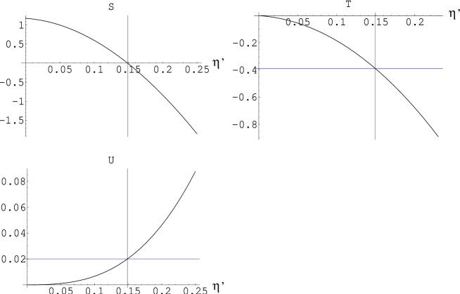
Figure 1: Plot of the oblique parameters as functions of the $B-L$ kinetic term on the TeV brane, normalized as $\eta^{\prime}=\tau^{\prime}/(R\log R^{\prime}/R)$. The grid lines point to the region where $S$ vanishes. These results include higher order corrections in the log and $\tau^{\prime}$ expansion, and we also checked them numerically.

The expressions obtained for $S,T,U$ are:

$$S \approx \frac{6\pi}{g^{2}\log\frac{R^{\prime}}{R}}-\frac{8\pi}{g^{2}}\left(1-\left(\frac{g^{\prime}}{g}\right)^{2}\right)\frac{\tau^{\prime 2}}{(R\log R^{\prime}/R)^{2}}~{},$$ (4.50)

$$T \approx -\frac{2\pi}{g^{2}}\left(1-\left(\frac{g^{\prime}}{g}\right)^{4}\right)\frac{\tau^{\prime 2}}{(R\log R^{\prime}/R)^{2}}~{},$$ (4.51)

$$U \approx 0~{}.$$ (4.52)

In this case, as $g^{\prime}/g=\tan\theta_{W}<1$, the additional contribution to $S$ is negative. This means that this contribution can cancel the positive log-suppressed result in Eq. (3.24). In Fig. 1 we plotted the numerical values of the oblique parameters, as functions of the properly normalized $B-L$ kinetic term. $S$ vanishes for $\tau^{\prime}/(R\log R^{\prime}/R)\approx 0.15$, a small value. We also find a negative contribution to $T$, that is $\approx-0.4$ when $S$ vanishes and a small contribution to $U$ from higher orders, $U\approx 0.02$. However, to T there will also be other moderate positive contributions of order $\sim 0.1$ at the loop level from the $t^{\prime},b^{\prime}$ sector.

Figure 2: The spectrum of the first three $Z$ resonances as a function of the $B-L$ kinetic term, normalized as $\eta^{\prime}=\tau^{\prime}/(R\log R^{\prime}/R)$.

It is now important to examine how the spectrum is changed. The $W$ resonances are clearly left unchanged, while in Fig. 2 we plotted the masses of the first three $Z$ resonances. The $Z$ mass is clearly left unchanged, being an imput parameter. However, the degeneracy of the first resonances originally at 1200 GeV is split. One boson is left stable around $1200$ GeV, while the other becomes light and if $S=0$ its mass drops to $\approx 300$ GeV. Increasing the $g_{5R}/g_{5L}$ mass ratio one can raise the Z^′ mass to about 400 GeV before perturbative unitarity is lost. In other words, this scenario predicts a light Z^′. Its couplings to the fermions are fixed by the wave function on the Planck brane:

$$g_{5}\psi_{Z^{\prime}}^{(L3)}(R)\,T_{3}+\tilde{g}_{5}\psi_{Z^{\prime}}^{(B)}(R)\,\frac{Y}{2}~{}.$$ (4.53)

We have numerically computed:

$$\frac{\psi_{Z^{\prime}}^{(L3)}(R)}{\psi_{Z}^{(L3)}(R)}\approx 0.03\,~{},\qquad\frac{\psi_{Z^{\prime}}^{(B)}(R)}{\psi_{Z}^{(B)}(R)}\approx 0.8\,~{},$$ (4.54)

so that our extra Z^′ mainly couples as a sequential hypercharge Z^′. Numerically, compared with the electric charge, the coupling is $\approx 0.2\,e\,Y/2$. This particular case is not fully covered in the literature [22], however the coupling should be small enough to escape direct production limits, mainly coming from the Tevatron (and also at LEP2). Another issue is the presence of induced 4-fermion couplings. Bounds on Z^′ masses vary between 150 and 800 GeV from 4 Fermi operators at HERA [23], depending on the precise structure and strength of the coupling of the extra Z^′ to SM fermions. However, the particular case of a sequential hypercharge Z^′ needs to be investigated in detail, which is beyond the scope of this paper.

5 Conclusions

We have calculated the tree-level oblique corrections to electroweak precision observables generated in higgless models of electroweak symmetry on a warped background. In the absence of brane induced kinetic terms (and equal left and right gauge couplings) we find the $S$ parameter to be $\sim 1.15$, while $T,U\sim 0$. Planck brane induced kinetic terms and unequal left-right couplings can lower $S$, however for sufficiently low values of $S$ tree-level unitarity will be lost. A kinetic term localized on the TeV brane for SU(2)_D will generically increase $S$, however an induced kinetic term for U(1)_B-L on the TeV brane will lower $S$. With appropriate choice of the value of this induced kinetic term $S\sim 0$ can be achieved. In this case the mass of the lowest Z^′ mode will be lowered to $\sim 300$ GeV.

References

- [1] N. Arkani-Hamed, S. Dimopoulos and G. R. Dvali, Phys. Lett. B 429, 263 (1998) [hep-ph/9803315].
- [2] L. Randall and R. Sundrum, Phys. Rev. Lett. 83, 3370 (1999) [hep-ph/9905221].
- [3] N. S. Manton, Nucl. Phys. B 158, 141 (1979); C. Csáki, C. Grojean and H. Murayama, Phys. Rev. D 67, 085012 (2003) [hep-ph/0210133]; C. A. Scrucca, M. Serone and L. Silvestrini, Nucl. Phys. B 669, 128 (2003) [hep-ph/0304220]; C. A. Scrucca, M. Serone, L. Silvestrini and A. Wulzer, hep-th/0312267.
- [4] N. Arkani-Hamed, A. G. Cohen, E. Katz and A. E. Nelson, JHEP 0207, 034 (2002) [hep-ph/0206021].
- [5] C. Csáki, C. Grojean, H. Murayama, L. Pilo and J. Terning, hep-ph/0305237.
- [6] R. S. Chivukula, D. A. Dicus and H. J. He, Phys. Lett. B 525, 175 (2002) [hep-ph/0111016]; R. S. Chivukula and H. J. He, Phys. Lett. B 532, 121 (2002) [hep-ph/0201164]; R. S. Chivukula, D. A. Dicus, H. J. He and S. Nandi, hep-ph/0302263; S. De Curtis, D. Dominici and J. R. Pelaez, Phys. Lett. B 554, 164 (2003) [hep-ph/0211353]; Phys. Rev. D 67, 076010 (2003) [hep-ph/0301059]; Y. Abe, N. Haba, Y. Higashide, K. Kobayashi and M. Matsunaga, hep-th/0302115.
- [7] K. Agashe, A. Delgado, M. J. May and R. Sundrum, JHEP 0308, 050 (2003) [hep-ph/0308036].
- [8] C. Csáki, C. Grojean, L. Pilo and J. Terning, hep-ph/0308038.
- [9] R. Barbieri, A. Pomarol and R. Rattazzi, hep-ph/0310285.
- [10] B. Holdom, Phys. Rev. D24 1441 (1981); B. Holdom, Phys. Lett. B150 301 (1985); K. Yamawaki, M. Bando, and K. Matumoto, Phys. Rev. Lett. 56 1335 (1986); T. Appelquist, D. Karabali, and L.C.R. Wijewardhana, Phys. Rev. Lett. 57 957 (1986); T. Appelquist and L.C.R. Wijewardhana, Phys. Rev. D35 774 (1987); T. Appelquist and L.C.R. Wijewardhana, Phys. Rev. D36 568 (1987).
- [11] Y. Nomura, JHEP 0311, 050 (2003) [hep-ph/0309189].
- [12] C. Csáki, C. Grojean, J. Hubisz, Y. Shirman and J. Terning, hep-ph/0310355.
- [13] T. Ohl and C. Schwinn, hep-ph/0312263.
- [14] J. Hirn and J. Stern, hep-ph/0401032.
- [15] R. Foadi, S. Gopalakrishna and C. Schmidt, hep-ph/0312324.
- [16] H. Davoudiasl, J. L. Hewett, B. Lillie and T. G. Rizzo, hep-ph/0312193.
- [17] G. Burdman and Y. Nomura, hep-ph/0312247.
- [18] C. Csáki, J. Erlich and J. Terning, Phys. Rev. D 66, 064021 (2002) [hep-ph/0203034].
- [19] M. Golden and L. Randall, Nucl. Phys. B361 (1991) 3; B. Holdom and J. Terning, Phys. Lett. B247 (1990) 88. M. E. Peskin and T. Takeuchi, Phys. Rev. D 46, 381 (1992).
- [20] K. Hagiwara et al. [Particle Data Group Collaboration], Phys. Rev. D 66, 010001 (2002).
- [21] J. Terning, Phys. Lett. B 344, 279 (1995) [hep-ph/9410233].
- [22] T. Appelquist, B. A. Dobrescu and A. R. Hopper, Phys. Rev. D 68, 035012 (2003) [hep-ph/0212073].
- [23] K. m. Cheung, Phys. Lett. B 517, 167 (2001) [hep-ph/0106251].