Cavendish-HEP-04/06 hep-ph/0401158

Renormalon approach to higher–twist distribution amplitudes and the convergence of the conformal expansion

Vladimir M. Braun¹, Einan Gardi^1,2 and Stefan Gottwald¹

¹Institut für Theoretische Physik, Universität Regensburg,
D-93040 Regensburg, Germany

² Cavendish Laboratory, University of Cambridge
Madingley Road, Cambridge, CB3 OHE, United Kingdom

Abstract:
Power corrections to exclusive processes are usually calculated using models for twist–four distribution amplitudes (DA) which are based on the leading–order terms in the conformal expansion. In this work we develop a different approach which does not rely on conformal symmetry but is based instead on renormalon analysis. This way we obtain an upper bound for the contributions of higher conformal spin operators, which translates into a bound on the end–point behavior of DA. The existence of such a bound is important for proving factorization theorems. For the two–particle twist–four DA we find in the renormalon model that the conformal expansion converges but it does not converge uniformly near the end points. This means that power corrections to observables which are particularly sensitive to the region where one valence quark is soft, may be underestimated when using the first few terms in the conformal expansion. The renormalon models of twist–four DA of the pion and the $\rho$ meson are constructed and can be used as a viable alternative to existing models.
Submitted to Nuclear Physics B

Keywords: QCD, Higher Twists, Exclusive Processes, Renormalons

1 Introduction

The relevant non-perturbative degrees of freedom in hard exclusive processes are described by hadron distribution amplitudes (DA) [1, 2] that detail the momentum–fraction distributions of partons in the infinite momentum frame by integrating out the transverse momentum dependence. The leading–twist parton distributions appear in the QCD description of hard exclusive reactions to the leading power accuracy and refer to parton configurations with the minimal number of constituents. The higher–twist distributions, in turn, are more numerous and are used to take into account a variety of effects due to parton virtuality, transverse momentum, and contributions of higher Fock states that are relevant for the description of power–suppressed corrections in the hard momentum. It should be mentioned that application of QCD factorization to exclusive processes beyond the leading–twist approximation presents a serious challenge because of end–point divergences related to the contributions of soft partons. Up to now such applications have been mostly in connection with the so–called light–cone sum rules (LCSR) [3] in which case the end–point divergences are removed by construction. More generally, end–point contributions have to be added and there is a hope that the precise separation of hard (twist–expandable) and soft (end–point) contributions can be achieved within the soft–collinear effective theory, see e.g. [4]. Having in mind the existing and potential applications it is worthwhile to have a fresh look at the theoretical description of higher–twist DA and the related uncertainties. The present work presents a step in this direction.

The existing theoretical framework for the description of DA is based on the conformal symmetry of the QCD Lagrangian, see [5] for a detailed review. The symmetry can be used to separate the dependence of the hadron wave function on the longitudinal momentum fractions and the transverse coordinates (that are later traded for the renormalization scale) in very much the same way as the rotational symmetry of the potential in quantum mechanics allows to separate the angular and the radial dependence. The orthogonal polynomials appearing in the expansion of distribution amplitudes [1, 2] are nothing but the irreducible representations of the collinear conformal group and play the same role as spherical harmonics in quantum mechanics, with the orbital angular momentum replaced by conformal spin. One motivation for using the conformal expansion is that contributions with different conformal spin do not mix with each other under QCD evolution to the leading logarithmic accuracy [1, 2]. Another rationale [6] is that QCD equations of motion (EOM) only relate terms with the same conformal spin so that any exact EOM–based relation between DA can be satisfied order by order in the conformal expansion. It follows that any parametrization of DA based on a truncated conformal expansion is consistent with the EOM and is preserved by evolution.

Assuming that DA are dominated by first few terms having the lowest conformal spin, the conformal expansion provides a practical framework for constructing models for DA [7, 8, 9, 10, 6, 11, 12, 13, 14, 15] which are both consistent with the QCD constraints and involve just a few non-perturbative parameters. This approach has been used extensively for phenomenology. Its main limitation is that just the first one or two terms in the expansion are included; the increasing number of parameters at higher conformal spins makes this program impractical otherwise, so the assumption that the conformal expansion converges fast is absolutely essential.

From the theoretical point of view, convergence of the conformal expansion is expected because anomalous dimensions of conformal operators are rising logarithmically with the spin and, therefore, higher–spin contributions are suppressed at asymptotically large scales. However, this suppression is numerically weak and not sufficient to guarantee convergence at the scales of practical interest. For leading twist this question can eventually be decided by experiment and indeed the qualitative success of quark counting rules and, more importantly, the CLEO data on the $\pi(\eta)\gamma\gamma^{*}$ transition form factor [16] strongly suggest that the meson DA are not very far from their asymptotic shape. For higher twist, using experimental data to constrain DA seems totally unrealistic and up to now there had been no arguments whatsoever whether truncation of the conformal expansion is legitimate in this case or not.

The aim of this work is to construct alternative models for twist–four meson DA that do not rely on the conformal expansion and present plausible bounds for the higher–spin contributions to these DA. To this end, we approach the problem from a different angle, using the concept of renormalons [17]. Owing to the breaking of scale invariance in the quantum theory through the running of the coupling, operators of different twist mix with each other under renormalization. Independence of a physical observable on the factorization scale implies intricate cancellations between different twists — the so–called cancellation of renormalon ambiguities — and the existence of these ambiguities can be used to estimate power–suppressed corrections in a similar way as the logarithmic scale dependence is used to estimate the accuracy of fixed–order perturbative calculations.

Most applications of renormalons have so far been in inclusive or semi–inclusive cross sections [17, 18], although some work has already been done in the context of exclusive processes. This includes analysis of the large–order behavior of the Brodsky–Lepage evolution kernel [19], and studies of infrared renormalons in specific processes, e.g. the $\gamma^{*}\gamma\pi_{0}$ form factor [20], the pion electromagnetic form factor [21], and deeply–virtual Compton scattering [22]. Here we do not consider a specific process but instead develop a general framework for estimating higher–twist contributions to exclusive processes involving pseudoscalar and vector mesons by constructing a renormalon model for DA, continuing the work by J. Andersen [23]. We trace the cancellation of renormalons and in this way establish an explicit connection between previous renormalon calculations and the operator product expansion (OPE) for exclusive processes, for cases that the latter exists. We then use the renormalon model to study the convergence of the conformal expansion.

In order to explain how the concept of renormalons becomes useful for constructing a consistent model for higher–twist DA let us discuss a concrete example. Consider the following matrix element:

$$\left\langle 0\left|{\rm T}\{\bar{d}(x_{2})\mbox{$\Delta$\raisebox{0.43057pt}{$/$}}\gamma_{5}u(x_{1})\}\right|\pi^{+}(p)\right\rangle_{\mu^{2}\simeq 1/|\Delta^{2}|}\,=\,$$ (1.1)

$$\hskip 1.0pt{}=i(p\Delta)\,f_{\pi}\!\int_{0}^{1}\!\!du\,{\rm e}^{-iupx_{1}-i\bar{u}px_{2}}\,\left[\int_{0}^{1}\!\!dv\,C(v,u,\Delta^{2},\mu_{F}^{2})\phi_{\pi}(v;\mu_{F}^{2})+\Delta^{2}g_{1}(u;\mu_{F}^{2})+\cdots\right]\!,$$

where $\bar{u}\equiv 1-u$, $f_{\pi}$ is the pion decay constant and the fields are taken at a small space-like separation: $\Delta\equiv x_{1}-x_{2}$ with $\Delta^{2}<0$, $|\Delta^{2}|\ll 1/\Lambda_{\rm QCD}^{2}$. Also, $\mu$ stands for the ultraviolet renormalization scale and for this discussion we assume that $\mu^{2}\simeq 1/|\Delta^{2}|$ to avoid large logarithms. The expansion in the square brackets on the right–hand side of Eq. (1.1) is nothing but the OPE: $C(v,u,\Delta^{2},\mu_{F}^{2})=\delta(u-v)+{\cal O}(\alpha_{s})$ is the twist–two coefficient function, $\phi_{\pi}(v;\mu_{F}^{2})$ is the standard, twist–two pion DA, and $\Delta^{2}g_{1}(u;\mu_{F}^{2})$ represents the twist–four contribution; $\mu_{F}^{2}$ is a factorization scale. The function $g_{1}(u;\mu_{F}^{2})$ can be interpreted as the distribution of the transverse momentum (squared) of the quark in the pion [10, 6] and is one example of the higher–twist DA that we will be interested in.

The conformal expansion of $g_{1}(u;\mu_{F}^{2})$ has been constructed in [6] using the expansion of three–particle DA involving a quark, an antiquark and a gluon, and EOM. In Sect. 4 we shall explain how this is done. Here we just quote the result:

$$g_{1}(u;\mu_{F}^{2}) = \bigg{\{}g^{(J=3)}(\mu_{F}^{2})\bigg{[}\,u^{2}\,\bar{u}^{2}\bigg{]}+g^{(J=4)}(\mu_{F}^{2})\bigg{[}u\bar{u}\,(13\,u\bar{u}+2)$$

$$+ 2\,(6\,u^{2}+3\,u+1)\,\bar{u}^{3}\,\mathrm{ln}(\bar{u})+2\,(6\,\bar{u}^{2}+3\,\bar{u}+1)\,\,u^{3}\mathrm{ln}(u)\bigg{]}+\cdots\bigg{\}},$$

where the coefficients $g^{(J)}(\mu_{F}^{2})$ renormalize multiplicatively, and $J=3,4,\ldots$ is the conformal spin. The corresponding logarithmic scale dependence cancels against the scale dependence of the twist–four coefficient function which is not shown in Eq. (1.1) for brevity. To the leading logarithmic accuracy and with the usual choice $\mu_{F}=\mu\simeq 1/|\Delta|$ this function reduces to a constant which can be included in the definition of $g_{1}(u;\mu_{F}^{2})$. The dots in Eq. (1) stand for the contribution of conformal spins $J\geq 5$, which were usually neglected. In this paper we want to study their significance.

To understand the rôle of renormalons one needs to carefully examine the separation made in Eq. (1.1) between twist two and twist four. For a qualitative discussion it is convenient to use a hard cutoff $1/|\Delta^{2}|\sim\mu^{2}\gg\mu_{F}^{2}\gg\Lambda^{2}$ for factorization: loop momenta $k^{2}>\mu_{F}^{2}$ contribute to the coefficient function $C(v,u,\Delta^{2},\mu_{F}^{2})$ while momenta $k^{2}<\mu_{F}^{2}$ contribute to the DA. Upon expanding the coefficient function near the light–cone $|\Delta^{2}|\mu_{F}^{2}\ll 1$, one obtains:

$$C(v,u,\Delta^{2},\mu_{F}^{2})=\bigg{(}1+c_{1}\alpha_{s}+c_{2}\alpha_{s}^{2}+\cdots\bigg{)}-d(v,u)\mu_{F}^{2}\Delta^{2}\cdots,$$ (1.3)

where $\alpha_{s}=\alpha_{s}(\mu^{2}=1/|\Delta^{2}|)$. It is the usual perturbative series with coefficients $c_{i}=c_{i}\left(v,u;\ln\left(\mu_{F}^{2}/\mu^{2}\right)\right)$ depending logarithmically on the scales, and the $d(v,u)$ term represents the leading power correction that arises because the low–momentum regions are cut off. Since the left–hand side of Eq. (1.1) does not depend on $\mu_{F}^{2}$, any such dependence in $C(v,u,\Delta^{2},\mu_{F}^{2})$ should cancel within the square brackets on the right–hand side. In particular, the logarithmic dependence of $C(v,u,\Delta^{2},\mu_{F}^{2})$ on $\mu_{F}^{2}$ is canceled by that of the twist–two distribution amplitude $\phi_{\pi}(v;\mu_{F}^{2})$. The cancellation of power dependence must involve the twist–four term $\Delta^{2}g_{1}(u;\mu_{F}^{2})$, so it is expected that in this factorization prescription

$$g_{1}(u;\mu_{F}^{2})\longrightarrow\mu_{F}^{2}\,\int_{0}^{1}dv\,d(v,u)\phi_{\pi}(v;\mu_{F}^{2})\,+\,\bar{g}_{1}(u;\mu_{F}^{2})\,,$$ (1.4)

where the second term depends on $\mu_{F}^{2}$ at most logarithmically. Indeed, upon renormalization the relevant twist–four operators show not only logarithmic ultraviolet divergence which is related to their anomalous dimension, but also quadratic ultraviolet divergence. Using a hard cutoff, the dependence of twist–four on $\mu_{F}^{2}$ is indeed that of Eq. (1.4): the twist–four operators mix with the leading–twist such that the dependence on $\mu_{F}^{2}$ in Eq. (1.1) cancels out. Clearly the function $d(v,u)$ can be computed either by considering the dependence of the twist–two coefficient function on $\mu_{F}^{2}$, i.e. its sensitivity to small loop momenta, or by considering the dependence of twist–four operators on $\mu_{F}^{2}$ i.e. their sensitivity to large loop momenta. Cancellation of $\mu_{F}^{2}$ to power accuracy requires that these two regularizations will be done using the same prescription.

In practice, a hard cutoff is difficult to implement. Usually, dimensional regularization is used instead. In this case power terms in the coefficient function (Eq. (1.3)) do not appear. However, the coefficients $c_{i}$ computed in a MS–like scheme diverge factorially with the order $i$. The factorial divergence implies that the sum of the perturbative series is only defined to a power accuracy and this ambiguity (renormalon ambiguity) must be compensated by adding a non-perturbative higher–twist correction. A detailed analysis shows [17] that the asymptotic large–order behavior of the coefficients (the renormalons) is in one–to–one correspondence with the sensitivity to extreme (small or large) loop momenta and that infrared renormalons in the leading–twist coefficient function are compensated by ultraviolet renormalons in the matrix elements of twist–four operators. At the end the picture described above re-appears: only the details depend on the factorization method.

Returning to Eq. (1.4) we observe that the quadratic term in $\mu_{F}$ is spurious since its sole purpose is to cancel the similar contribution to the coefficient function. It does not contribute, therefore, to any physical observable. The idea of the renormalon model [17, 18] is that, with a replacement of $\mu_{F}$ by a suitable non-perturbative scale, this contribution should be of the same order and have roughly the same functional form as the physical second contribution on the right–hand side of Eq. (1.4), which is the only one of interest. Assuming this “ultraviolet dominance” [24, 25, 17] we get the following model:

$$g_{1}(u;\mu_{F}^{2})\simeq k\Lambda_{\rm QCD}^{2}\,\int_{0}^{1}dv\,d(v,u)\phi_{\pi}(v;\mu_{F}^{2}),$$ (1.5)

where by explicit calculation (see Sect. 2) one finds for $d(v,u)$ at leading order

$$d(v,u) = \frac{1}{v^{2}}\,\bigg{[}u+(v-u)\ln\left(1-\frac{u}{v}\right)\bigg{]}\theta(v>u)$$ (1.6)

$$\hskip 40.0pt+\,\frac{1}{(1-v)^{2}}\,\bigg{[}1-u+(u-v)\ln\left(1-\frac{1-u}{1-v}\right)\bigg{]}\theta(v<u).$$

The overall coefficient in this model $k={\cal O}(1)$ can be fixed by the normalization integral $\int_{0}^{1}du\,g_{1}(u;\mu^{2})$ corresponding to the matrix element of a local operator which can be estimated by QCD sum rules [10, 6] or calculated on the lattice. To the accuracy of Eq. (1.6) the logarithmic $\mu_{F}$ dependence on the left–hand side and on the right–hand side of Eq. (1.5) do not match: one expects this model to be relevant at low scales of the order of a few times $\Lambda_{\rm QCD}$.

The “ultraviolet dominance” assumption used to derive Eq. (1.5), is in fact sufficient to derive the full set of two– and three–particle DA of twist–four in terms of the leading–twist DA. It is important that this approximation is fully consistent with the OPE and respects all constraints imposed by EOM. On the other hand, it does not assume any hierarchy of contributions of the increasing conformal spin and indeed the expressions in Eq. (1) and Eq. (1.5) are very different for any reasonable choice of the leading–twist DA. Since twist–four anomalous dimensions are not taken into account, one should expect that this model overestimates contributions of conformal operators with high spin. It is therefore complementary to the usual models based on using a first few terms with the lowest spin and provides an upper–bound estimate of the neglected contributions.

The presentation is organized as follows. In Sect. 2 we formulate our program in more precise terms, introducing the relevant techniques (Borel transform) and the systematic approximation (large–$N_{f}$ expansion) that will be used throughout the rest of the work. The expression in Eq. (1.6) is derived and the cancellation of the renormalon ambiguity for the matrix element of the type in Eq. (1.1) is demonstrated by an explicit calculation. The renormalon model of the pion DA of twist–four is presented in Sect. 3 and in Sect. 4 we discuss its conformal expansion. The generalization of these results for the case of vector mesons is considered in Sect. 5 while Sect. 6 is reserved for the conclusions.

2 Cancellation of renormalon ambiguities in the OPE

2.1 Definitions

In this section we compute the renormalon ambiguity of the leading–twist coefficient function in the simplest exclusive amplitude involving a pseudoscalar meson, and demonstrate how the unique result is restored by adding the twist–four contributions in the OPE. To begin with, let us set up the necessary definitions.

We choose to consider the gauge–invariant time–ordered product of two quark “currents” at a small (but non-vanishing) light–cone separation, which can be parametrized in terms of two Lorentz–invariant amplitudes $G_{1}(u,\Delta^{2};\mu^{2})$ and $G_{2}(u,\Delta^{2};\mu^{2})$ defined as

$$\left\langle 0\left|{\rm T}\{\bar{d}(x_{2})\gamma_{\nu}\gamma_{5}[x_{2},x_{1}]u(x_{1})\}\right|\pi^{+}(p)\right\rangle_{\mu^{2}}\,=\,$$ (2.1)

$$\hskip 40.0pt=i\,f_{\pi}\,\int_{0}^{1}\,du\,{\rm e}^{-iupx_{1}-i\bar{u}px_{2}}\,\left[G_{1}(u,\Delta^{2};\mu^{2})p_{\nu}+G_{2}(u,\Delta^{2};\mu^{2})\left(\frac{p\cdot\Delta}{\Delta^{2}}\Delta_{\nu}-p_{\nu}\right)\right].$$

Here $\Delta\equiv x_{1}-x_{2}$ with $|\Delta^{2}|\ll 1/\Lambda_{\rm QCD}^{2}$, $\Delta^{2}<0$ playing the rôle of the hard scale, $\bar{u}=1-u$ and $\mu^{2}$ is the ultraviolet renormalization scale. We use the notation $[x_{2},x_{1}]$ for the Wilson line connecting the points $x_{2}$ and $x_{1}$,

$$[x_{2},x_{1}]=P\exp\left[-ig\int_{0}^{1}\!dt\,\Delta_{\mu}A^{\mu}(x_{2}+t\Delta)\right].$$ (2.2)

Note that the $\mu^{2}$ dependence comes entirely from the wave–function renormalization of the quark and the antiquark fields in Eq. (2.1) and can be removed by adding the corresponding $Z$–factors. Up to this additional renormalization, the functions $G_{1,2}(u,\Delta^{2};\mu^{2})$ can be viewed as physical amplitudes. Their advantage is that they are simpler than exclusive amplitudes which are relevant for phenomenology (such as the two–photon one) and at the same time retain all the features that are important in the present context.

The asymptotic behavior of $G_{i}(u,\Delta^{2};\mu^{2})$, $i=1,2$ in the light–cone limit $\Delta^{2}\longrightarrow 0$ with $\Delta\cdot p$ fixed can be studied by the OPE, schematically

$$G_{i}(u,\Delta^{2})=C_{i}^{(2)}\otimes\phi^{(2)}\,+\,\Delta^{2}\sum C_{i}^{(4)}\otimes\phi_{i}^{(4)}\,+\,{\cal O}(\Delta^{4}),$$ (2.3)

where $C_{i}^{(t)}$ are the coefficient functions and $\phi^{(t)}$ are the pion DA given by vacuum–to–pion matrix elements of renormalized non-local operators, $t$ refers to twist and the summation goes over all independent contributions of given twist. The convolution is defined as

$$C_{i}\otimes\phi=\int_{0}^{1}dv\,C_{i}(v,u,\Delta^{2},\mu^{2},\mu_{F}^{2})\,\phi(v;\mu_{F}^{2}),$$ (2.4)

where $u,v$ have the meaning of the light–cone momentum fractions and we have indicated the dependence on the factorization scale $\mu_{F}^{2}$ and other variables. The Lorentz structures in Eq. (2.1) are chosen such that the coefficient functions $C_{i}$ depend on $\Delta^{2}$ logarithmically as follows from power counting.

The leading–twist pion DA $\phi_{\pi}(u)=\phi^{(2)}(u)$ is defined as usual by

$$\left\langle 0\left|\bar{d}(-z)\not\!z\gamma_{5}[-z,z]u(z)\right|\pi^{+}(p)\right\rangle_{\mu_{F}^{2}} = if_{\pi}(pz)\,\int_{0}^{1}du\,{\rm e}^{-ipz(u-\bar{u})}\phi_{\pi}(u;\mu_{F}^{2})\,,$$ (2.5)

where the normalization condition is

$$\int_{0}^{1}du\,\phi_{\pi}(u;\mu_{F}^{2})=1.$$ (2.6)

Here and below $z_{\mu}$ is the light–like vector, $z^{2}=0$. Although we will usually be using covariant notation, it is sometimes convenient to refer to light–cone coordinates where $p=(p_{+},0,0)$ and $x=(0,x_{-},x_{\perp})$. The light–cone limit corresponds to $x_{\perp}\longrightarrow 0$ with $x_{-}$ fixed such that $z=(0,x_{-},0)$.

In the present paper we will consider the leading–twist coefficient function to all orders in $\alpha_{s}(\mu^{2})$ but restrict ourselves to the leading order in higher–twist contributions: $C^{(4)}(u,v)=\delta(u-v)+{\cal O}(\alpha_{s})$. To this accuracy there is a single twist–four DA contributing to each of the functions $G_{1,2}$:

$$G_{1}(u,\Delta^{2}) = \bigg{[}1+c_{1}\alpha_{s}+c_{2}\alpha_{s}^{2}+\cdots\bigg{]}\otimes\phi_{\pi}+\Delta^{2}\phi_{1}^{(4)}(u;\mu_{F}^{2})+\cdots$$

$$G_{2}(u,\Delta^{2}) = \bigg{[}\widetilde{c}_{1}\alpha_{s}+\widetilde{c}_{2}\alpha_{s}^{2}+\cdots\bigg{]}\otimes\phi_{\pi}+\Delta^{2}\phi_{2}^{(4)}(u;\mu_{F}^{2})+\cdots.$$ (2.7)

In physical terms $\phi^{(4)}_{1}(u;\mu_{F}^{2})$ and $\phi^{(4)}_{2}(u;\mu_{F}^{2})$ correspond to contributions of valence–quark transverse momenta and of the “wrong” components of the quark spinors, respectively. In the notations of Ref. [6]

$$g_{1}(u)=\phi_{1}^{(4)}(u)\qquad\qquad{\rm and}\qquad\qquad g_{2}(u)=\frac{d}{du}\phi_{2}^{(4)}(u).$$

For an operator definition, it is convenient to use the concept of non-local operator off the light cone [26] which is defined as the generating function (formal Taylor expansion) for renormalized local operators. For example,

$$\Big{[}\bar{d}(-x)\not\!x\gamma_{5}[-x,x]u(x)\Big{]}_{\mu_{F}^{2}} = \sum_{k}\frac{2^{k+1}}{k!}x_{\nu}x_{\nu_{1}}\ldots x_{\nu_{k}}\bigg{\{}\Big{[}d\gamma_{\nu}\stackrel{{\scriptstyle\leftrightarrow}}{{D}}_{\nu_{1}}\ldots\stackrel{{\scriptstyle\leftrightarrow}}{{D}}_{\nu_{1}}u-\mbox{\rm Traces}\Big{]}_{\mu_{F}^{2}}^{\rm twist-2}$$ (2.8)

$$+\big{[}\mbox{\rm Traces}\big{]}^{\rm twist-4}_{\mu_{F}^{2}}+\big{[}\mbox{\rm Traces}\big{]}^{\rm twist-6}_{\mu_{F}^{2}}+\ldots\bigg{\}},$$

where $\stackrel{{\scriptstyle\leftrightarrow}}{{D}}_{\nu_{1}}=\stackrel{{\scriptstyle\rightarrow}}{{D}}_{\nu_{1}}-\stackrel{{\scriptstyle\leftarrow}}{{D}}_{\nu_{1}}$ is the covariant derivative, see [26, 27] for details. Note that the twist expansion of a non-local operator corresponds to its expansion over irreducible representations of the Lorentz group. This involves rearrangement of traces and symmetrization over groups of indices if necessary, cf. [28]. This compact notation is widely used in [6, 10, 11, 26, 13, 15]. In particular, we have [6]

$$\langle 0|\Big{[}\bar{d}(x_{2})\gamma_{\nu}\gamma_{5}[x_{2},x_{1}]u(x_{1})\}\Big{]}_{\mu_{F}^{2}}|\pi^{+}(p)\rangle\,=\,$$

$$\hskip 30.0pt=i\,f_{\pi}p_{\nu}\int_{0}^{1}du\,{\rm e}^{-iupx_{1}-i\bar{u}px_{2}}\left[\phi^{(2)}(u;\mu_{F}^{2})+\Delta^{2}\phi^{(4)}_{1}(u;\mu_{F}^{2})+{\cal O}(\Delta^{4})\right]$$

$$\hskip 40.0pt+\,i\,f_{\pi}\Big{(}\Delta_{\nu}(p\Delta)-p_{\nu}\Delta^{2}\Big{)}\int_{0}^{1}du\,{\rm e}^{-iupx_{1}-i\bar{u}px_{2}}\left[\phi^{(4)}_{2}(u;\mu_{F}^{2})+{\cal O}(\Delta^{2})\right].$$ (2.9)

Despite the similar appearance, beyond the tree level Eq. (2.1) and Eq. (2.1) describe different objects. As follows from the Taylor expansion Eq. (2.8) the non–local operator on the left–hand side of Eq. (2.1) is an analytic function of $\Delta^{2}$ at $\Delta^{2}\longrightarrow 0$. It corresponds to the analytic part of the amplitude in Eq. (2.1) [27] while the coefficient functions (by definition) take into account singular contributions. The most striking difference is that the non-local operator in Eq. (2.1) does not include the whole twist–two part of $G_{2}(u,\Delta^{2})$ in Eq. (2.1), which is $\sim 1/\Delta^{2}$. This contribution was overlooked in [23]. The non-local operator also does not include any of the coefficient functions appearing in Eq. (2.1), which absorb all logarithms $\sim\ln(-\Delta^{2}\mu_{F}^{2})$.

Using the EOM the two–particle pion DA $\phi^{(4)}_{1}(u;\mu_{F}^{2})$ and $\phi^{(4)}_{2}(u;\mu_{F}^{2})$ can be expressed in terms of the Fock components involving an extra gluon field. Following [6] we define the three–particle pion DA of twist four

$$\left\langle 0\left|\bar{d}(-z)[-z,vz]\gamma_{\nu}\gamma_{5}gG_{\mu\rho}(vz)[vz,z]u(z)\right|\pi^{+}(p)\right\rangle\,=\,\,$$

$$\hskip 35.0pt=\,f_{\pi}\int\!{\cal D}\alpha_{i}\,\,{\rm e}^{-ipz(\alpha_{1}-\alpha_{2}+\alpha_{3}v)}\bigg{\{}\frac{p_{\nu}}{pz}\,(p_{\mu}z_{\rho}-p_{\rho}z_{\mu})\Phi_{\parallel}(\alpha_{1},\alpha_{2},\alpha_{3})$$

$$\hskip 60.0pt+\left[\,p_{\rho}\left(g_{\mu\nu}-\frac{z_{\mu}p_{\nu}}{pz}\right)-p_{\mu}\left(g_{\rho\nu}-\frac{z_{\rho}p_{\nu}}{pz}\right)\right]\Phi_{\perp}(\alpha_{1},\alpha_{2},\alpha_{3})\bigg{\}},$$ (2.10)

where the longitudinal momentum fraction of the gluon is $\alpha_{3}$ and the integration measure is defined as

$$\int\!{\cal D}\alpha_{i}=\int_{0}^{1}d\alpha_{1}d\alpha_{2}d\alpha_{3}\,\delta(1-\alpha_{1}-\alpha_{2}-\alpha_{3})\,.$$ (2.11)

One obtains [6] (see also Appendix A in [12]):

$$\phi_{2}^{(4)}(u) = \int_{0}^{u}dv\int_{0}^{v}d\alpha_{1}\int_{0}^{1-v}d\alpha_{2}\,\frac{1}{\alpha_{3}}\left[2\Phi_{\perp}-\Phi_{\parallel}\right](\alpha_{1},\alpha_{2},\alpha_{3})$$

$$\phi_{1}^{(4)}(u)+\phi_{2}^{(4)}(u) = \frac{1}{2}\int_{0}^{u}d\alpha_{1}\int_{0}^{1-u}d\alpha_{2}\,\frac{\bar{u}\alpha_{1}-u\alpha_{2}}{\alpha_{3}^{2}}\left[2\Phi_{\perp}-\Phi_{\parallel}\right](\alpha_{1},\alpha_{2},\alpha_{3}),$$

where $\alpha_{3}=1-\alpha_{1}-\alpha_{2}$. The derivation of these relations relies on exact operator identities [26] which relate integrals over $v$ of the quark–gluon–antiquark operator in Eq. (2.1) to derivatives of the quark–antiquark operator appearing in Eq. (2.1).

For completeness, we present here the definitions of the other three–particle twist–four pion DA. These distributions do not contribute to Eq. (2.1) to leading order because of our specific choice of the (simple) correlation function, but are important for other applications. We will use these definitions in Sect. 3 where we construct the renormalon model.

First of all, there exist another pair of DA that correspond to the substitution of $\gamma_{5}G_{\mu\rho}$ by $i\widetilde{G}^{\mu\rho}\equiv\frac{i}{2}\epsilon^{\mu\rho\alpha\beta}G_{\alpha\beta}$ in Eq. (2.1). To the twist–four accuracy

$$\langle 0|\bar{d}(-z)[-z,vz]\gamma_{\nu}ig\widetilde{G}_{\mu\rho}(vz)[vz,z]u(z)|\pi^{+}(p)\rangle\,=\,\,$$ (2.13)

$$\hskip 35.0pt=\,f_{\pi}\int\!{\cal D}\alpha_{i}\,\,{\rm e}^{-ipz(\alpha_{1}-\alpha_{2}+\alpha_{3}v)}\bigg{\{}\frac{p_{\nu}}{pz}\,(p_{\mu}z_{\rho}-p_{\rho}z_{\mu})\Psi_{\parallel}(\alpha_{1},\alpha_{2},\alpha_{3})$$

$$\hskip 60.0pt+\left[\,p_{\rho}\left(g_{\mu\nu}-\frac{z_{\mu}p_{\nu}}{pz}\right)-p_{\mu}\left(g_{\rho\nu}-\frac{z_{\rho}p_{\nu}}{pz}\right)\right]\Psi_{\perp}(\alpha_{1},\alpha_{2},\alpha_{3})\bigg{\}}.$$

The functions $\Psi_{\perp,\parallel}$ and $\Phi_{\perp,\parallel}$ are not independent. In particular $\Psi_{\perp}$ and $\Phi_{\perp}$ can be obtained as the symmetric and the antisymmetric part, respectively, of a more general DA [13]

$$\langle 0|\bar{d}(-z)[-z,vz]\gamma_{-}\gamma_{\nu}\gamma_{+}ig\widetilde{G}_{\mu\rho}(vz)[vz,z]u(z)|\pi^{+}(p)\rangle\,=\,\,$$ (2.14)

$$=\,f_{\pi}\left[\,p_{\rho}\left(g_{\mu\nu}-\frac{z_{\mu}p_{\nu}}{pz}\right)-p_{\mu}\left(g_{\rho\nu}-\frac{z_{\rho}p_{\nu}}{pz}\right)\right]\int\!{\cal D}\alpha_{i}\,\,{\rm e}^{-ipz(\alpha_{1}-\alpha_{2}+\alpha_{3}v)}H^{\downarrow\uparrow}(\alpha_{1},\alpha_{2},\alpha_{3})\,.$$

One obtains [13]

$$\Psi_{\perp}(\alpha_{1},\alpha_{2},\alpha_{3})=-\frac{1}{2}\left[H^{\downarrow\uparrow}(\alpha_{1},\alpha_{2},\alpha_{3})+H^{\downarrow\uparrow}(\alpha_{2},\alpha_{1},\alpha_{3})\right],$$

$$\Phi_{\perp}(\alpha_{1},\alpha_{2},\alpha_{3})=-\frac{1}{2}\left[H^{\downarrow\uparrow}(\alpha_{1},\alpha_{2},\alpha_{3})-H^{\downarrow\uparrow}(\alpha_{2},\alpha_{1},\alpha_{3})\right],$$ (2.15)

see also Appendix A in [30].

In addition, we introduce a new three–particle DA $\Xi_{\pi}(\alpha_{i})$ as

$$\left\langle 0\left|\bar{d}(-z)\gamma_{\mu}\gamma_{5}gD^{\alpha}G_{\alpha\beta}(vz)[vz,z]u(z)\right|\pi^{+}(p)\right\rangle=$$

$$\hskip 60.0pt=\,if_{\pi}p_{\mu}p_{\beta}\int\!{\cal D}\alpha_{i}\,\,{\rm e}^{-ipz(\alpha_{1}-\alpha_{2}+v\alpha_{3})}\,\Xi_{\pi}(\alpha_{1},\alpha_{2},\alpha_{3}).$$ (2.16)

The Lorentz structure $p_{\mu}p_{\beta}$ is the only one relevant at twist four. Thanks to the equation of motion $D^{\alpha}G^{A}_{\alpha\beta}=-g\sum_{q}\bar{q}t^{A}\gamma_{\beta}q$ where the summation goes over all light flavors, $\Xi_{\pi}(\alpha_{i})$ can be viewed as describing either a quark–antiquark–gluon or a specific four–quark component of the pion: with the quark–antiquark pair in a color–octet state and at the same space–time point. This DA was not considered previously because its conformal expansion starts with a higher spin $J=5$ (see below) whereas in [6, 13] only the terms with $J=3$ and $J=4$ were included.

There exist further twist–four four–quark operators where all quark light–cone coordinates are separated, and also twist–four operators which include two gluons in addition to the quark–antiquark pair. They give rise to four–particle DA and will not be considered in this work. Although such operators contribute to exclusive amplitudes at twist four, they do not appear to leading order in the flavor expansion (cf. [31]) and can be systematically neglected to our accuracy.

2.2 Infrared renormalons in the twist–two coefficient functions

The scale separation made in Eq. (2.3) is arbitrary in two respects. To a given logarithmic accuracy  the separation between coefficient functions and operator matrix elements is ambiguous. However, the logarithmic dependence on the factorization scale $\mu_{F}^{2}$ cancels between the coefficient function $C^{(t=2)}$ and the corresponding DA $\phi^{(t=2)}$ leaving their product invariant. This can be phrased through perturbative evolution equations. To power accuracy  the separation between terms of different twist is ambiguous and the scale–independence of “structure functions” $G$ is only restored in the sum of all twists.

As discussed in the introduction the intuitive way to see this is to imagine using a cutoff scale $\mu_{F}^{2}$ to implement factorization: this scale serves as an infrared cutoff for the coefficient functions while it acts as an ultraviolet cutoff for the DA. The twist–two contribution would then depend on the scale as $\sim\mu_{F}^{2}\Delta^{2}\phi^{(2)}$. To keep $G$ invariant this dependence should cancel against a term of the form $\mu_{F}^{2}\phi^{(2)}$ in $\phi_{i}^{(4)}$. In other words, the twist–four operator has a quadratic ultraviolet divergence through which it mixes with the twist–two operator. In dimensional regularization the power–like cutoff dependence does not occur, but the ambiguity still persists because the perturbative series develops a factorial large–order behaviour. The perturbation theory, therefore, diverges (renormalon divergence) and its sum is only defined to power–like accuracy. This is the renormalon ambiguity which we are going to address now.

2.2.1 An all–order calculation

In order to evaluate the infrared–renormalon ambiguity in the twist–two coefficient functions

$$C_{1}^{(2)}(v,u,\Delta^{2},\mu^{2},\mu_{F}^{2}) = \delta(u-v)+c_{1}\alpha_{s}(\mu^{2})+c_{2}\alpha_{s}^{2}(\mu^{2})+\cdots$$

$$C_{2}^{(2)}(v,u,\Delta^{2},\mu^{2},\mu_{F}^{2}) = \widetilde{c}_{1}\alpha_{s}(\mu^{2})+\widetilde{c}_{2}\alpha_{s}^{2}(\mu^{2})+\cdots$$ (2.17)

we need to calculate them to all orders in the coupling. Of course, a full all–order calculation cannot be performed. Instead, as in other applications [17], we restrict ourselves to the perturbative series generated by the running–coupling effects in one–loop diagrams, i.e. using QCD coupling at the scale of the gluon virtuality. A convenient tool to perform this calculation is the Borel representation of the running coupling,

$$\frac{\beta_{0}\alpha_{s}(-k^{2})}{\pi}=\int_{0}^{\infty}dw\,{\rm e}^{\frac{5}{3}w}\,\left(\frac{\Lambda^{2}}{-k^{2}}\right)^{w},$$ (2.18)

where $\beta_{0}$ is the leading–order coefficient of the $\beta$ function,

$$\frac{d(\alpha_{s}/\pi)}{d\ln\mu^{2}}=-\beta_{0}(\alpha_{s}/\pi)^{2}+\ldots\hskip 60.0pt\beta_{0}=\frac{11}{12}C_{A}-\frac{1}{6}N_{f}\,,$$ (2.19)

$\Lambda=\Lambda_{\rm QCD}^{\overline{\rm{MS}}}$ and the exponential factor ${\rm e}^{\frac{5}{3}w}$ originates from the renormalization of the fermion loop in the $\overline{\rm{MS}}$ scheme. This way the calculation reduces to one loop with a modified gluon propagator

$$\frac{1}{-k^{2}}\longrightarrow\frac{(\Lambda^{2})^{w}}{(-k^{2})^{1+w}}.$$ (2.20)

and the result for the coefficient functions takes the form of a Borel integral

$$C_{1}(v,u,\Delta^{2},\mu^{2},\mu_{F}^{2}) = \delta(u-v)\,+\,\int_{0}^{\infty}dw\,{\rm e}^{\frac{5}{3}w}\,B_{1}(w;v,u,\Delta^{2}\mu^{2},\mu_{F}^{2}/\mu^{2})\,\left(-\Delta^{2}\Lambda^{2}\right)^{w},$$

$$C_{2}(v,u,\Delta^{2},\mu^{2},\mu_{F}^{2}) = \int_{0}^{\infty}dw\,{\rm e}^{\frac{5}{3}w}\,B_{2}(w;v,u,\Delta^{2}\mu^{2},\mu_{F}^{2}/\mu^{2})\,\left(-\Delta^{2}\Lambda^{2}\right)^{w}.$$ (2.21)

The perturbative expansion of $C_{i}$ can be recovered order by order from the expansion of their Borel transforms $B_{i}$ near $w=0$ observing that for one–loop coupling

$$\int_{0}^{\infty}\,dw\,w^{n}\left(\Lambda^{2}/\mu^{2}\right)^{w}=\frac{n!}{\left(\ln\mu^{2}/\Lambda^{2}\right)^{n+1}}=n!\left(\alpha_{s}\beta_{0}/\pi\right)^{n+1}.$$

The fixed–sign factorial behavior of the coefficients in this expansion in high orders manifests itself in that the functions $B_{i}$ develop singularities at finite values of $w$ on the positive real axis (renormalon singularities) rending the integrals in Eq. (2.21) ill–defined. The imaginary part that arises when the integration contour is moved above (or below) of the nearest singularity (to the origin) can be taken as a measure of the ambiguity of the summation of the perturbative series, see [17] for details.

The relevant diagrams are shown in Fig. 1.

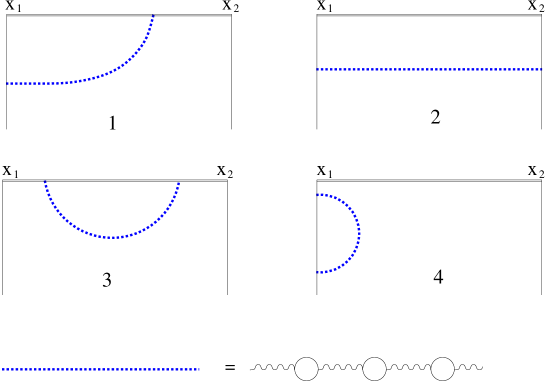
Figure 1: One–loop diagrams appearing in the non-local matrix element of Eq. (2.1). The upper double line represents a path–ordered exponential (a Wilson line) connecting $x_{1}$ and $x_{2}$, while the dashed line represents a dressed gluon (dressing is equivalent to summing over any number of fermion–loops insertions in the large–$N_{f}$ limit).

The calculation is presented in detail in Appendix A. We consider quarks on–shell and set the space-time dimension to $d=4$ from the beginning since $w\not=0$ acts as a regulator. The result for the (not yet renormalized) coefficient functions reads

$$B_{1}(w;u,v) = \frac{C_{F}}{2\beta_{0}}\frac{\Gamma(-w)}{\Gamma(1+w)}4^{-w}\bigg{\{}\theta(u>v)\frac{1}{\bar{v}}\left[(1+w)f_{+}^{(w)}\left(1-\frac{\bar{u}}{\bar{v}}\right)-wf^{(w)}\left(1-\frac{\bar{u}}{\bar{v}}\right)\right]$$ (2.22)

$${}\hskip 75.0pt+\,\theta(u<v)\frac{1}{v}\left[(1+w)f_{+}^{(w)}\left(1-\frac{u}{v}\right)-wf^{(w)}\left(1-\frac{u}{v}\right)\right]$$

$${}\hskip 75.0pt+\,\frac{1-w}{1+w}\left[\theta(u>v)\left(\frac{\bar{u}}{\bar{v}}\right)^{w+1}+\theta(u<v)\left(\frac{u}{v}\right)^{w+1}\right]$$

$$\hskip 75.0pt{}-\,\frac{1}{1-2w}\delta(u-v)\bigg{\}}$$

and

$$B_{2}(w;u,v) = \frac{C_{F}}{\beta_{0}}\frac{\Gamma(1-w)}{\Gamma(2+w)}4^{-w}\left[\theta(u>v)\left(\frac{\bar{u}}{\bar{v}}\right)^{w+1}+\theta(v>u)\left(\frac{u}{v}\right)^{w+1}\right],$$ (2.23)

where we used a short–hand notation

$$f^{(w)}(\beta) = \frac{\beta^{2w-1}(1-\beta)^{1+w}}{1+w}\,_{2}\!F_{1}(2w,w+1,2+w;1-\beta)\,.$$ (2.24)

In particular

$$f^{(w=0)}(\beta) = \frac{1-\beta}{\beta},$$

$$f^{(w=1)}(\beta) = 1-\beta+\beta\ln\beta\,.$$ (2.25)

The “$+$” prescription is defined as usual by:

$$f^{(w)}_{+}(\beta)=f^{(w)}(\beta)-\delta(\beta)\int_{0}^{1}d\tilde{\beta}f^{(w)}(\tilde{\beta}).$$ (2.26)

The terms $\sim f^{(w)}$ in Eq. (2.22) correspond, in Feynman gauge, to the contribution of the vertex correction (Diagram 1) in Fig. 1 and its symmetric counterpart, the contribution in the third line in Eq. (2.22) and the entire Eq. (2.23) originate from the box diagram (Diagram 2) and the remaining term $\sim 1/(1-2w)$ in the last line of Eq. (2.22) stands for the self–energy insertion in the Wilson line (Diagram 3).

2.2.2 Singularities of the Borel transform

The answer for $B_{1}(w;u,v)$ in Eq. (2.22) has a simple pole at $w=0$. This singularity is expected [17] and has to be removed by the subtraction of ultraviolet (UV) logarithmic divergences due to the wave–function renormalization of the quark fields, and of infrared (IR) logarithmic divergences that correspond to the renormalization of the leading–twist DA. To this end, note that vanishing of the Diagram 4 in Fig. 1 is a result of an exact cancellation between IR and UV divergent integrals. Upon introducing a scale which regulates one singularity, the other one will appear as a $1/w$ pole. Schematically

$$B_{1}(w;u,v)^{\rm Diagram-4}=\frac{C_{F}}{4\beta_{0}}\left(\left[\frac{1}{w}\right]_{\hbox{\tiny UV}}-\left[\frac{1}{w}\right]_{\hbox{\tiny IR}}\right).$$ (2.27)

In addition to renormalizing Diagram 4, ultraviolet subtraction removes the $1/w$ pole of Diagram 3 in Fig. 1.

Having performed the UV renormalization the remaining $1/w$ singularities from Diagrams 1, 2 and 4 are removed upon performing IR factorization. The counter-term which is to be subtracted from the DA $\phi^{(2)}$ and added to the coefficient function $B_{1}(w;u,v)$ is

$$B_{1}(w;u,v)^{\rm c.t.}=\frac{C_{F}}{2\beta_{0}}\frac{K(u,v)+{\cal O}(w)}{w}$$ (2.28)

where $K(u,v)$ is obtained as the limit at $w\to 0$ of the expression in the curly brackets in Eq. (2.22) and adding the IR–pole contribution in Eq. (2.27):

$$K(u,v)\equiv\left[\frac{v}{u}\left(1+\frac{1}{u-v}\right)\theta(u>v)+\frac{1-v}{1-u}\left(1+\frac{1}{v-u}\right)\theta(u<v)\right]_{+}.$$ (2.29)

$K(u,v)$ can easily be identified as the leading–order Brodsky–Lepage kernel [1, 2] controlling the $\mu_{F}^{2}$–evolution of the pion DA $\phi_{\pi}(u;\mu_{F}^{2})$:

$$\frac{d\phi_{\pi}(v;\mu_{F}^{2})}{d\ln\mu_{F}^{2}}=\frac{C_{F}\alpha_{s}}{2\pi}\int_{0}^{1}du\,K(u,v)\,\phi_{\pi}(u;\mu_{F}^{2})\,.$$ (2.30)

The terms ${\cal O}(w)$ in Eq. (2.28) correspond to scheme–dependent higher–order contributions to the Brodsky–Lepage evolution kernel. In MS–like schemes the kernel has an expansion in $\alpha_{s}$ with a finite radius of convergence, see [19] for explicit expressions in the large–$\beta_{0}$ limit. In other words in such schemes the infrared counter-term is free of Borel singularities.

To summarize, the subtraction of logarithmic UV and IR divergences removes the $1/w$ singularity in the Borel transformed coefficient functions in much the same way as poles $1/(d-4)$ are subtracted in renormalized amplitudes when using dimensional regularization. For the subsequent discussion it is important that in MS-like schemes the subtracted terms are analytic functions of the Borel variable $w$ and do not influence the structure of singularities of $B_{i}$ at $w>0$ which we are going to address now. For this reason we can work with non-subtracted amplitudes in what follows.

First, we note the presence of a Borel singularity at $w=1/2$ in the last term in Eq. (2.22) which comes from the self-energy insertion in the Wilson line and reflects a linear divergence in the UV region (UV renormalon). Such singularities are well–known in the context of the heavy–quark effective theory [32] in which case they reflect ambiguities in the non-perturbative definition of the heavy–quark mass [33, 32]. In our case, this singularity is an artifact of choosing an oversimplified “exclusive process” in Eq. (2.1) where a dynamical quark propagating between the points $x_{1}$ and $x_{2}$ is replaced by a path–ordered exponential. It has nothing to do with the twist expansion and will not appear in realistic physics applications. Therefore we will not consider this singularity further in this paper.

The remaining singularities at positive integer $w_{0}=1,2,\ldots$ have IR origin and are called IR renormalons. They obstruct the Borel integration in Eq. (2.21) and render the sum of perturbation theory ambiguous to power accuracy $\sim(\Lambda^{2}\Delta^{2})^{w_{0}}$. Hence we concentrate on the IR renormalon with $w_{0}=1$ which is the closest one to the origin and the only one relevant for the calculation to the twist–four accuracy $\sim\Delta^{2}$. For definiteness, we choose the residue at the $w=1$ singularity times $\pi=3.14\ldots$ as a measure of the ambiguity of the Borel integral (2.21), i.e.

$$\delta_{\hbox{\tiny IR}}\left\{\frac{f(w)}{1-w}\right\}=-\pi f(w=1)\,.$$ (2.31)

Using Eq. (2.22) and Eq. (2.23) we obtain the ambiguity of the twist–two approximation for the amplitudes $G_{1}$ and $G_{2}$

$$\delta_{\hbox{\tiny IR}}\left\{C_{1}\otimes\phi_{\pi}\right\} = -c\Lambda^{2}\Delta^{2}\!\!\int_{0}^{1}\!\!dv\,\phi_{\pi}(v)\left\{\frac{1}{v}\,f^{(1)}\left(1\!-\!\frac{u}{v}\right)\theta(v>u)\right.\left.+\,\frac{1}{\bar{v}}\,f^{(1)}\left(1\!-\!\frac{\bar{u}}{\bar{v}}\right)\theta(v<u)\right\}$$

$$= -c\Lambda^{2}\Delta^{2}\!\!\int_{0}^{1}\!\!dv\,\phi_{\pi}(v)\bigg{\{}\frac{1}{v^{2}}\,\bigg{[}u+(v-u)\ln\left(1-\frac{u}{v}\right)\bigg{]}\theta(v>u)$$

$$\hskip 90.0pt+\,\frac{1}{\bar{v}^{2}}\,\bigg{[}\bar{u}+(u-v)\ln\left(1-\frac{\bar{u}}{\bar{v}}\right)\bigg{]}\theta(v<u)\bigg{\}},$$

$$\delta_{\hbox{\tiny IR}}\left\{C_{2}\otimes\phi_{\pi}\right\} = c\Lambda^{2}\Delta^{2}\int_{0}^{1}dv\,\phi_{\pi}(v)\left\{\left(\frac{u}{v}\right)^{2}\theta(v>u)+\left(\frac{\bar{u}}{\bar{v}}\right)^{2}\theta(v<u)\right\},$$ (2.32)

respectively, where we used Eq. (2.2.1) and where the overall normalization

$$c\equiv\frac{\pi C_{F}}{8\beta_{0}}{\rm e}^{\frac{5}{3}}\simeq 0.7$$ (2.33)

corresponds to the convention in Eq. (2.31). The given number is for $N_{F}=3$. We are going to demonstrate that this ambiguity is exactly canceled by the UV renormalon ambiguity in the twist–four DA, which is reminiscent of quadratic UV divergence of the contributing operators.

2.3 UV renormalons in higher–twist operators and cancellation of ambiguities

In order to reveal the UV–renormalon divergence in the twist–four DA we consider the perturbative series generated by running–coupling effects in the matrix element of a generic quark–antiquark–gluon operator

$$\bar{d}(-z)[-z,vz]\Gamma gG_{\alpha\beta}(vz)[vz,z]u(z),$$ (2.34)

sandwiched between quarks states with momenta $q_{1}$ and $q_{2}$ with $q_{i}^{2}\not=0$. Here $\Gamma$ stands for an arbitrary Dirac structure and $z^{2}=0$. The relevant diagrams are shown in Fig. 2.

Figure 2: One–loop diagrams appearing in the non-local matrix element of quark–antiquark–gluon light–cone operators. The upper double line represents a path–ordered exponential (a Wilson line) along the light cone connecting between $-z$ and $vz$ and between $vz$ and $z$ while the dashed line represents a dressed gluon (dressing is equivalent to summing over any number of fermion–loops insertions in the large–$N_{f}$ limit).

One obtains

$$\left\langle q_{2}\left|\bar{d}(-z)\Gamma gG_{\alpha\beta}(vz)u(z)\right|q_{1}\right\rangle = {\rm e}^{-i(q_{1}+q_{2})z}\,\left(g_{\lambda\alpha}g_{\beta}^{\mu}-g_{\lambda\beta}g_{\alpha}^{\mu}\right)\frac{4\pi^{2}C_{F}}{\beta_{0}}\,\,\int_{0}^{\infty}\!\!dw\,{\rm e}^{\frac{5}{3}w}(-\Lambda^{2})^{w}\,$$ (2.35)

$${}\times\Big{[}\bar{d}_{q_{2}}\gamma_{\mu}\gamma_{\rho}\Gamma u_{q_{1}}\,I^{\lambda\rho}(q_{2},(1+v)z)-\bar{d}_{q_{2}}\Gamma\gamma_{\rho}\gamma_{\mu}u_{q_{1}}\,I^{\lambda\rho}(q_{1},(1-v)z)\Big{]},$$

where $\bar{d}_{q_{2}}$ and $u_{q_{1}}$ are quark spinors and $I^{\lambda\rho}(q,z)$ stands for the momentum integral

$$I^{\lambda\rho}(q,z)=\int\frac{d^{4}k}{(2\pi)^{4}}\frac{k^{\lambda}(q+k)^{\rho}}{\left(k^{2}\right)^{(1+w)}(q+k)^{2}}\,{\rm e}^{-ikz}$$ (2.36)

which is UV divergent at $w=1$. Performing the integral and extracting the $w=1$ pole, we obtain:

$$\left.I^{\lambda\rho}(q,z)\right|_{w=1} = \frac{-i}{32\pi^{2}(1-w)}\,\int_{0}^{1}\!da\,a\,{\rm e}^{iqz(1-a)}$$ (2.37)

$${}\times\bigg{[}iq^{\lambda}z^{\rho}(1-a)-iq^{\rho}z^{\lambda}a+g^{\lambda\rho}+\frac{1}{2}a(1-a)q^{2}z^{\lambda}z^{\rho}\bigg{]}.$$

As a consequence of the $w=1$ singularity the Borel integral in Eq. (2.35) is ill–defined. Using Eq. (2.31) to quantify the ambiguity and specifying for the relevant Dirac and Lorentz structures the final result can be brought to a form of operator relations (cf. [17, 23])

$$\delta_{\hbox{\tiny UV}}\left\{z^{\mu}\,\bar{d}(-z)\gamma^{\nu}\gamma_{5}gG_{\mu\nu}(vz)u(z)\right\} = 2i\,c\Lambda^{2}\int_{0}^{1}\!da\,(1-a)\Big{[}\bar{d}(-y)\mbox{$z$\raisebox{0.43057pt}{$/$}}\gamma_{5}u(z)-\bar{d}(-z)\mbox{$z$\raisebox{0.43057pt}{$/$}}\gamma_{5}u(\widetilde{y})\Big{]},$$

$$\delta_{\hbox{\tiny UV}}\left\{z^{\mu}\,\bar{d}(-z)\mbox{$z$\raisebox{0.43057pt}{$/$}}\gamma_{5}gG_{\mu\rho}(vz)u(z)\right\} = -2i\,c\Lambda^{2}\,z_{\rho}\int_{0}^{1}da\,a\,\Big{[}\bar{d}(-y)\mbox{$z$\raisebox{0.43057pt}{$/$}}\gamma_{5}u(z)-\bar{d}(-z)\mbox{$z$\raisebox{0.43057pt}{$/$}}\gamma_{5}u(\widetilde{y})\Big{]},$$

$$\delta_{\hbox{\tiny UV}}\left\{z^{\mu}\bar{d}(-z)\gamma^{\nu}ig\widetilde{G}_{\mu\nu}(vz)u(z)\right\} = 2i\,c\Lambda^{2}\int_{0}^{1}\!da\,(1+a)\,\Big{[}\bar{d}(-y)\mbox{$z$\raisebox{0.43057pt}{$/$}}\gamma_{5}u(z)+\bar{d}(-z)\mbox{$z$\raisebox{0.43057pt}{$/$}}\gamma_{5}u(\widetilde{y})\Big{]},$$

$$\delta_{\hbox{\tiny UV}}\left\{z^{\mu}\bar{d}(-z)\mbox{$z$\raisebox{0.43057pt}{$/$}}ig\widetilde{G}_{\mu\rho}(vz)u(z)\right\} = 2i\,c\Lambda^{2}z_{\rho}\int_{0}^{1}da\,a\,\Big{[}\bar{d}(-y)\mbox{$z$\raisebox{0.43057pt}{$/$}}\gamma_{5}u(z)+\bar{d}(-z)\mbox{$z$\raisebox{0.43057pt}{$/$}}\gamma_{5}u(\widetilde{y})\Big{]},$$

where $y\equiv z(1-(1+v)(1-a))$ and $\widetilde{y}\equiv z(1-(1-v)(1-a))$, and $c$ is the constant defined in Eq. (2.33). In order to arrive at these expressions we performed integration by parts over $a$ in order to remove factors of $q\cdot z$ and then converted the results into operator relations in configuration space. The relations in Eq. (2.3) can be viewed as the mixing under renormalization between the twist–four quark–gluon–antiquark operators and the twist–two quark–antiquark operator and the first two of them were derived in [23]. In a similar manner — see Appendix B — we obtain one more operator relation

$$\delta_{\hbox{\tiny UV}}\left\{\bar{d}(-z)z^{\beta}gD^{\alpha}G_{\alpha\beta}(vz)\mbox{$z$\raisebox{0.43057pt}{$/$}}\gamma_{5}u(z)\right\}=$$ (2.39)

$$= -4ic\Lambda^{2}\int_{0}^{1}da\,a\frac{d}{da}\left[\frac{1}{1+v}\,\bar{d}(-y)\mbox{$z$\raisebox{0.43057pt}{$/$}}\gamma_{5}u(z)\,+\,\frac{1}{1-v}\bar{d}(-z)\mbox{$z$\raisebox{0.43057pt}{$/$}}\gamma_{5}u(\widetilde{y})\right].$$

Taking matrix elements of Eqs. (2.3) and (2.39) between the vacuum and the pion state we derive UV ambiguities of three–particle pion DA defined in Sect. 2.1 in terms of the leading–twist pion DA:

$$\delta_{\hbox{\tiny UV}}\left\{\Phi_{\perp}(\alpha_{1},\alpha_{2},\alpha_{3})\right\} = c\Lambda^{2}\left[\frac{\phi_{\pi}(\alpha_{1})}{1-\alpha_{1}}-\frac{\phi_{\pi}(\alpha_{2})}{1-\alpha_{2}}\right],$$

$$\delta_{\hbox{\tiny UV}}\left\{\Phi_{\parallel}(\alpha_{1},\alpha_{2},\alpha_{3})\right\} = 2c\Lambda^{2}\left[\frac{\alpha_{2}\phi_{\pi}(\alpha_{1})}{(1-\alpha_{1})^{2}}-\frac{\alpha_{1}\phi_{\pi}(\alpha_{2})}{(1-\alpha_{2})^{2}}\right],$$

$$\delta_{\hbox{\tiny UV}}\left\{\Psi_{\perp}(\alpha_{1},\alpha_{2},\alpha_{3})\right\} = c\Lambda^{2}\left[\frac{\phi_{\pi}(\alpha_{1})}{1-\alpha_{1}}+\frac{\phi_{\pi}(\alpha_{2})}{1-\alpha_{2}}\right],$$

$$\delta_{\hbox{\tiny UV}}\left\{\Psi_{\parallel}(\alpha_{1},\alpha_{2},\alpha_{3})\right\} = -2c\Lambda^{2}\left[\frac{\alpha_{2}\phi_{\pi}(\alpha_{1})}{(1-\alpha_{1})^{2}}+\frac{\alpha_{1}\phi_{\pi}(\alpha_{2})}{(1-\alpha_{2})^{2}}\right],$$

$$\delta_{\hbox{\tiny UV}}\left\{\Xi_{\pi}(\alpha_{1},\alpha_{2},\alpha_{3})\right\} = -4c\Lambda^{2}\left[\frac{\alpha_{2}\,\phi_{\pi}(\alpha_{1})}{1-\alpha_{1}}-\frac{\alpha_{1}\,\phi_{\pi}(\alpha_{2})}{1-\alpha_{2}}\right],$$ (2.40)

where we used the symmetry property $\phi_{\pi}(\alpha)=\phi_{\pi}(1-\alpha)$ to arrive at the given expressions.

Last but not least, we use EOM in Eq. (2.1) to calculate the UV–renormalon ambiguity in the two–particle twist–four pion DA $\phi_{1,2}^{(4)}$ and find that it coincides identically with the IR renormalon ambiguity of the twist–two result in Eq. (2.2.2) but has opposite sign. It follows that the “structure functions” $G_{i}$ are unambiguous to the twist–four accuracy

$$\delta\left\{G_{1}\right\} = \delta_{\hbox{\tiny IR}}\left\{C_{1}\otimes\phi_{\pi}\right\}+\Delta^{2}\delta_{\hbox{\tiny UV}}\left\{\phi_{1}^{(4)}\right\}=0\,,$$

$$\delta\left\{G_{2}\right\} = \delta_{\hbox{\tiny IR}}\left\{C_{2}\otimes\phi_{\pi}\right\}+\Delta^{2}\delta_{\hbox{\tiny UV}}\left\{\phi_{2}^{(4)}\right\}=0\,,$$ (2.41)

as expected. For the cancellation to hold, it is important that both the leading–twist coefficient functions and the matrix elements of higher–twist operators are calculated using the same regularization and renormalization prescription. This can be seen as a consistency check for the OPE analysis.

3 Renormalon model for twist–four DA of the pion

The UV–renormalon ambiguities in the twist–four DA should be viewed as indicative of the size and the momentum–fraction dependence of “genuine” non-perturbative effects. We define the renormalon model for twist–four DA of the pion by taking the functional form of the corresponding UV–renormalon ambiguities, replacing the overall normalization constant $c\Lambda^{2}$ by a suitable non-perturbative parameter. The crucial observation is that although the absolute normalization of the renormalon ambiguity in Eq. (2.31) is essentially ad hoc, the relative normalization for the different DA in Eq. (2.3) is meaningful since the running–coupling calculation satisfies all constraints imposed by Lorentz symmetry and the EOM. Therefore, the renormalon model for the entire set of twist–four DA of the pion has just one free parameter: the overall normalization. This parameter can be related to the matrix element of the local operator

$$\langle 0|\bar{d}\gamma_{\nu}ig\widetilde{G}_{\mu\rho}u|\pi^{+}(p)\rangle\,=\,\frac{1}{3}f_{\pi}\delta^{2}[p_{\rho}g_{\mu\nu}-p_{\mu}g_{\rho\nu}]\,,\qquad\delta^{2}\simeq 0.2~{}\mbox{GeV}^{2},$$ (3.1)

where the number comes from QCD sum rules [34]. The UV–renormalon ambiguity of the same matrix element is, on the other hand

$$\delta_{\hbox{\tiny UV}}\left\{\langle 0|\bar{d}\gamma_{\nu}ig\widetilde{G}_{\mu\rho}u|\pi^{+}(p)\rangle\right\}\,=\,2f_{\pi}c\Lambda^{2}[p_{\rho}g_{\mu\nu}-p_{\mu}g_{\rho\nu}]\,,$$ (3.2)

so in Eq. (2.3) we replace

$$c\Lambda^{2}\to\frac{1}{6}\delta^{2}\simeq(180~{}\mbox{\rm MeV})^{2}$$ (3.3)

and end up with the set of three–particle DA

$$\Phi_{\perp}(\alpha_{1},\alpha_{2},\alpha_{3}) = \frac{\delta^{2}}{6}\left[\frac{\phi_{\pi}(\alpha_{1})}{1-\alpha_{1}}-\frac{\phi_{\pi}(\alpha_{2})}{1-\alpha_{2}}\right],$$

$$\Phi_{\parallel}(\alpha_{1},\alpha_{2},\alpha_{3}) = \frac{\delta^{2}}{3}\left[\frac{\alpha_{2}\phi_{\pi}(\alpha_{1})}{(1-\alpha_{1})^{2}}-\frac{\alpha_{1}\phi_{\pi}(\alpha_{2})}{(1-\alpha_{2})^{2}}\right],$$

$$\Psi_{\perp}(\alpha_{1},\alpha_{2},\alpha_{3}) = \frac{\delta^{2}}{6}\left[\frac{\phi_{\pi}(\alpha_{1})}{1-\alpha_{1}}+\frac{\phi_{\pi}(\alpha_{2})}{1-\alpha_{2}}\right],$$

$$\Psi_{\parallel}(\alpha_{1},\alpha_{2},\alpha_{3}) = -\frac{\delta^{2}}{3}\left[\frac{\alpha_{2}\phi_{\pi}(\alpha_{1})}{(1-\alpha_{1})^{2}}+\frac{\alpha_{1}\phi_{\pi}(\alpha_{2})}{(1-\alpha_{2})^{2}}\right],$$

$$\Xi_{\pi}(\alpha_{1},\alpha_{2},\alpha_{3}) = -\frac{2\delta^{2}}{3}\left[\frac{\alpha_{2}\,\phi_{\pi}(\alpha_{1})}{1-\alpha_{1}}-\frac{\alpha_{1}\,\phi_{\pi}(\alpha_{2})}{1-\alpha_{2}}\right].$$ (3.4)

Note that we have made the same replacement in all five DA. It must be so because these DA are all related — see Appendix B. Using the EOM, Eq. (3), (cf. Eq. (2.2.2)),

$$\phi_{1}^{(4)}(u) = \frac{\delta^{2}}{6}\!\!\int_{0}^{1}\!\!dv\,\phi_{\pi}(v)\bigg{\{}\frac{1}{v^{2}}\,\bigg{[}u+(v-u)\ln\left(1-\frac{u}{v}\right)\bigg{]}\theta(v>u)$$

$$\hskip 90.0pt+\,\frac{1}{\bar{v}^{2}}\,\bigg{[}\bar{u}+(u-v)\ln\left(1-\frac{\bar{u}}{\bar{v}}\right)\bigg{]}\theta(v<u)\bigg{\}},$$

$$\phi_{2}^{(4)}(u) = -\frac{\delta^{2}}{6}\int_{0}^{1}dv\,\phi_{\pi}(v)\left\{\left(\frac{u}{v}\right)^{2}\theta(v>u)+\left(\frac{\bar{u}}{\bar{v}}\right)^{2}\theta(v<u)\right\}$$ (3.5)

which completes the calculation.

The given expressions are valid for an arbitrary leading–twist pion DA $\phi_{\pi}(u)$. For practical applications it may be worthwhile to choose the asymptotic expression

$$\phi_{\pi}(u)=6u(1-u)$$ (3.6)

which is known to provide one with a reasonable accuracy [16]. With this choice

$$\Phi_{\perp}(\alpha_{1},\alpha_{2},\alpha_{3}) = \delta^{2}[\alpha_{1}-\alpha_{2}]\,,$$

$$\Phi_{\parallel}(\alpha_{1},\alpha_{2},\alpha_{3}) = 2\delta^{2}\alpha_{1}\alpha_{2}\left[\frac{1}{1-\alpha_{1}}-\frac{1}{1-\alpha_{2}}\right]\,,$$

$$\Psi_{\perp}(\alpha_{1},\alpha_{2},\alpha_{3}) = \delta^{2}\left[\alpha_{1}+\alpha_{2}\right]\,,$$

$$\Psi_{\parallel}(\alpha_{1},\alpha_{2},\alpha_{3}) = -2\delta^{2}\alpha_{1}\alpha_{2}\left[\frac{1}{1-\alpha_{1}}+\frac{1}{1-\alpha_{2}}\right]\,,$$

$$\Xi_{\pi}(\alpha_{1},\alpha_{2},\alpha_{3}) = 0\,.$$ (3.7)

Note that $\Xi_{\pi}(\alpha_{1},\alpha_{2},\alpha_{3})$ is vanishing in this approximation, but in general it is not zero and has to be taken into account if corrections to the asymptotic pion DA are included.

For the two particle DA one gets [23]

$$\phi_{1}^{(4)}(u) = \delta^{2}\bigg{\{}\bar{u}\bigg{[}\ln(\bar{u})-\mbox{\rm Li}_{2}(\bar{u})\bigg{]}+u\bigg{[}\ln(u)-\mbox{\rm Li}_{2}(u)\bigg{]}-u\bar{u}+\frac{\pi^{2}}{6}\bigg{\}},$$

$$\phi_{2}^{(4)}(u) = \delta^{2}\,\bigg{\{}u^{2}\ln(u)+\bar{u}^{2}\ln(\bar{u})+u\bar{u}\bigg{\}},$$ (3.8)

where ${\rm Li}_{a}(x)\equiv\sum_{n=1}^{\infty}x^{n}/n^{a}$. In the next section we shall compare these expressions with the model of [6, 13] based on conformal expansion.

4 Conformal expansion

4.1 General formalism

For fields “living” on the light–cone the conformal transformations reduce to the three–parameter group $SL(2,\mathbb{R})$ with the algebra of hyperbolic rotations, see [5] for a review. The conformal transformations for quantum fields are governed by their conformal spin which is defined as

$$j=\frac{1}{2}(s+\ell)\,,$$ (4.1)

where $\ell$ is the scaling dimension, $\ell=3/2$ for quarks and $\ell=1$ for gluons, and $s$ is the spin projection on the light cone. For Dirac spinors (quarks) the different spin components can be separated with the help of projection operators $q_{\pm}=\Pi_{\pm}q$ where

$$\Pi_{+}=\frac{1}{2}\gamma{-}\gamma{+},\qquad\qquad\Pi_{-}=\frac{1}{2}\gamma{+}\gamma{-},\qquad\qquad\Pi_{+}+\Pi_{-}=1\,.$$ (4.2)

The $q_{+}$ and $q_{-}$ fields have spin projections $s=1/2$ and $s=-1/2$, and hence different conformal spins $j=1$ and $j=1/2$, respectively. Similarly, the gluon field strength has to be decomposed in different spin components: $G_{+\perp}$ has spin projection $s=1$ and conformal spin $j=3/2$; $G_{\perp\perp}$ and $G_{+-}$ both have $s=0$ and $j=1$; finally $G_{-\perp}$ has $s=-1$ and $j=1/2$.

Conformal expansion of DA presents an example of the classical problem of spin summation in quantum mechanics, with the only difference being that the total conformal spin $J$ of the multi-parton system is always larger or equal to the sum of spins of constituents:

$$J=J_{\rm min}+N\,,\qquad J_{\rm min}=j_{1}+\ldots+j_{k}\,.$$ (4.3)

The integer number $N$ can be identified with the total number of covariant derivatives $D_{+}$ in the corresponding local operator. Adding a derivative increases the conformal spin by one unit and does not change the twist of the operator, defined as dimension minus spin. The generic conformal expansion for two–particle DA has the form [36]

$$\phi(u)=\frac{\Gamma(2j_{1}+2j_{2})}{\Gamma(2j_{1})\Gamma(2j_{2})}\,u^{2j_{1}-1}\,(1-u)^{2j_{2}-1}\,\sum_{N=0}^{\infty}\,c_{J}\,P^{(2j_{1}-1,2j_{2}-1)}_{N}(2u-1)\,,$$ (4.4)

where $P_{N}^{(\alpha,\beta)}[x]$ are Jacobi polynomials [35], $u$ and $1-u$ stand for the momentum fractions of the parton with spin $j_{1}$ and $j_{2}$, respectively, and the coefficients $c_{J}$ correspond to the contribution of the total conformal spin $J=j_{1}+j_{2}+N$. The factor in front of the sum is called the asymptotic distribution amplitude.

For three partons, a generic DA can be written as a double sum

$$\Phi(\alpha_{i})=\frac{\Gamma(2j_{1}+2j_{2}+2j_{3})}{\Gamma(2j_{1})\Gamma(2j_{2})\Gamma(2j_{3})}\,\alpha_{1}^{2j_{1}-1}\,\alpha_{2}^{2j_{2}-1}\,\alpha_{3}^{2j_{3}-1}\,\sum_{N=0}^{\infty}\,\sum_{n=0}^{N}\,C_{Jj}\,Y_{Jj}^{(12)3}(\alpha_{i})\,,$$ (4.5)

where [37, 38]

$$\!\!\!Y_{Jj}^{(12)3}(\alpha_{i})=(1-\alpha_{3})^{j-j_{1}-j_{2}}\,P_{J-j-j_{3}}^{(2j_{3}-1,2j-1)}[1-2\alpha_{3}]\,P_{j-j_{1}-j_{2}}^{(2j_{1}-1,2j_{2}-1)}\left[\frac{\alpha_{2}-\alpha_{1}}{1-\alpha_{3}}\right]$$ (4.6)

are the basis functions [5] corresponding to the total conformal spin $J=j_{1}+j_{2}+j_{3}+N$ and the fixed conformal spin of the $(1,2)$–parton pair $j=j_{1}+j_{2}+n$. The functions $Y_{Jj}^{(12)3}(\alpha_{i})$ form a complete basis and are mutually orthogonal with respect to the conformal scalar product:

$$\int_{0}^{1}{\cal D}\alpha_{i}\,\,\alpha_{1}^{2j_{1}-1}\alpha_{2}^{2j_{2}-1}\alpha_{3}^{2j_{3}-1}\,Y_{Jj}^{(12)3}(\alpha_{i})Y_{J^{\prime}j^{\prime}}^{(12)3}(\alpha_{i})={\cal N}_{Jj}\,\delta_{JJ^{\prime}}\,\delta_{jj^{\prime}}\,,$$ (4.7)

where

$${\cal N}_{Jj} = \frac{\Gamma(j\!+\!j_{1}\!-\!j_{2})\Gamma(j\!-\!j_{1}\!+\!j_{2})}{\Gamma(j\!-\!j_{1}\!-\!j_{2}\!+\!1)\Gamma(j\!+\!j_{1}\!+\!j_{2}\!-\!1)(2j\!-\!1)}\,\frac{\Gamma(J\!-\!j\!+\!j_{3})\Gamma(J\!+\!j\!-\!j_{3})}{\Gamma(J\!-\!j\!-\!j_{3}\!+\!1)\Gamma(J\!+\!j\!+\!j_{3}\!-\!1)(2J\!-\!1)}\,.$$

Using this orthogonality property the coefficients in the expansion of any DA can be obtained by projection:

$$C_{Jj} = \frac{\Gamma(2j_{1})\Gamma(2j_{2})\Gamma(2j_{3})}{\Gamma(2j_{1}+2j_{2}+2j_{3})}\,\frac{1}{{\cal N}_{Jj}}\,\int_{0}^{1}{\cal D}\alpha_{i}\,\Phi(\alpha_{i})\,Y_{Jj}^{(12)3}(\alpha_{i}).$$ (4.9)

The use of conformal symmetry is that, for a given twist, only the coefficients $C_{J,j}$ with $j_{1}+j_{2}\leq j\leq J-j_{3}$ in Eq. (4.5) and $c_{J}$ in Eq. (4.4) for the same value of the total spin  $J$ can be related by EOM and/or renormalization group evolution to the leading logarithmic accuracy. It follows that any parametrization of DA based on a truncated conformal expansion is consistent with the EOM and is preserved by evolution.

4.2 The two lowest orders

The relevant light–cone projections of the twist–four light–cone operators corresponding to the three–particle pion DA are

$${\cal H}^{\downarrow\uparrow}_{\perp} = \bar{d}_{-}(-z)\gamma^{\perp}\gamma_{5}gG_{\perp+}(vz)u_{+}(z)\,,$$

$${\cal O}_{\parallel} = \bar{d}_{+}(-z)\gamma_{+}\gamma_{5}gG_{+-}(vz)u_{+}(z)\,,$$

$$\widetilde{\cal O}_{\parallel} = \bar{d}_{+}(-z)\gamma_{+}ig\widetilde{G}_{+-}(vz)u_{+}(z)\,,$$

$${\cal D} = \bar{d}_{+}(-z)\gamma_{+}\gamma_{5}gD^{\mu}G_{\mu+}(vz)u_{+}(z)\,.$$ (4.10)

In the first operator $j_{d}=\frac{1}{2}$, $j_{u}=1$ and $j_{g}=3/2$ while in the second and the third operators $j_{d}=1$, $j_{u}=1$ and $j_{g}=1$. In all these cases the sum is the same, $J=j_{d}+j_{u}+j_{g}=3$. This is the minimum conformal spin corresponding to the asymptotic DA. In the fourth operator $j_{d}=j_{u}=1$ but owing to the derivative $j_{g}=2$, making the minimal conformal spin $4$. In addition, the $G$–parity demands that DA $\Phi_{\parallel}$ and $\Xi_{\pi}$ are antisymmetric under the interchange of $\alpha_{1}\leftrightarrow\alpha_{2}$. This implies that the matrix elements of the operators with minimal conformal spin vanish identically in these two cases and the conformal expansion for $\Phi_{\parallel}$ and $\Xi_{\pi}$ starts one unit of spin higher at $J=4$ and $J=5$, respectively.

The model developed in [6, 13] corresponds to taking into account contributions of the lowest two conformal spins $J=3$ and $J=4$. To this accuracy

$$\Phi_{\perp}(\alpha_{1},\alpha_{2},\alpha_{3}) = 10\,\delta^{2}\,(\alpha_{1}-\alpha_{2})\alpha_{3}^{2}\left[1+6\,\epsilon\,(1-2\alpha_{3})\right]\,,$$

$$\Phi_{\parallel}(\alpha_{1},\alpha_{2},\alpha_{3}) = 120\epsilon\delta^{2}\alpha_{1}\alpha_{2}\alpha_{3}(\alpha_{1}-\alpha_{2})\,,$$

$$\Psi_{\perp}(\alpha_{1},\alpha_{2},\alpha_{3}) = 10\delta^{2}\alpha_{3}^{2}(1-\alpha_{3})\left[1+6\epsilon(1-2\alpha_{3})\right]\,,$$

$$\Psi_{\parallel}(\alpha_{1},\alpha_{2},\alpha_{3}) = -40\delta^{2}\alpha_{1}\alpha_{2}\alpha_{3}\left[1+3\epsilon(1-3\alpha_{3})\right]\,,$$

$$\Xi_{\pi}(\alpha_{1},\alpha_{2},\alpha_{3}) = 0\,.$$ (4.11)

      

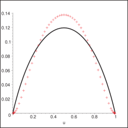
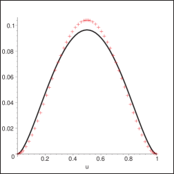
Figure 3: The two–particle twist–four DA $\phi_{1}^{(4)}$ (left) and $-\phi_{2}^{(4)}$ (right) based on the renormalon model (full line) and model of Ref. [6] (crosses) which uses the first two orders in the conformal expansion with the sum–rule estimate $\epsilon=0.5$. The normalization is chosen to be the same $\delta=1$.

The terms $\sim\delta^{2}$ are $J=3$ and define the asymptotic DA while contributions $\sim\epsilon\delta^{2}$ correspond to $J=4$. For each spin $J=3$ and $J=4$ there exists only one independent non-perturbative parameter and from conformal symmetry it follows that they have to have an autonomous scale dependence. This can be checked by a direct computation.

We have defined an alternative, renormalon model of higher–twist DA in Sect. 3 by requiring that it reproduces the correct normalization in Eq. (3.1). It is now a matter of a simple algebra to expand the renormalon model in Eq. (3) in contributions of increasing conformal spin (4.5) and compare with Eq. (4.2). We find that the structure in Eq. (4.2) is reproduced and the parameter $\epsilon$ proves to be independent on the choice of the leading–twist pion DA. One obtains

$$\left.\epsilon\right|_{\rm Ren}={7}/{12}\simeq 0.58$$ (4.12)

which is comfortably close to the QCD sum–rule estimate

$$\left.\epsilon\right|_{\rm SR}\simeq 0.5\pm 0.1\quad\mbox{\cite[cite]{[\@@bibref{}{BF90}{}{}]}}\,.$$ (4.13)

It is important that the conformal expansion of all four DA in Eq. (4.5) yields the same value of $\epsilon$, which illustrates that the renormalon model is consistent with the EOM. Note that $\Xi_{\pi}(\alpha_{1},\alpha_{2},\alpha_{3})=0$ to this accuracy; as mentioned above, its conformal expansion starts with $J=5$.

The two–particle twist–four DA of Eq. (2.3) are related to the three–particle ones through the EOM, Eq. (2.1). Thus, when truncated to order $J=4$ in the conformal expansion, the renormalon model essentially coincides with the model of [6], with the sole difference being the replacement of the sum–rule estimate for $\epsilon$ in Eq. (4.13), by that in Eq. (4.12). However, in the renormalon model there is a priori no need to truncate the expansion at $J=4$:  Eq. (3) represents the sum of all conformal spins. Figure 3 compares the two–particle DA between the model of [6] and that of Eq. (3). In general the two models are close, especially for $\phi_{2}^{(4)}$. We note, however, a qualitative difference in the end–point behavior. This is the subject of the next section.

4.3 Higher orders and the end–point behavior

4.3.1 Three–particle distributions

Let us start with the three–particle functions. The difference between the models in Eq. (3) and Eq. (4.2) corresponds to the contribution of higher conformal spins $J\geq 5$. Most striking is that the end–point behavior of the renormalon model expressions for small gluon momenta $\alpha_{3}\equiv\alpha_{g}\to 0$ is $\Phi\sim{\it const}$ for all five three–particle distributions in question whereas for each order in the conformal expansion $\Phi_{\parallel},\Psi_{\parallel}\sim\alpha_{3}^{1}$, $\Phi_{\perp},\Psi_{\perp}\sim\alpha_{3}^{2}$ and $\Xi_{\pi}\sim\alpha_{3}^{3}$.

The difference indicates that the conformal expansion is not converging. Indeed, assuming the asymptotic leading–twist pion DA in Eq. (3.6) we derive the following formal expansion of the DA in Eq. (3) in contributions of the conformal spin $J$:

$$\left\{\begin{array}[]{c}\Psi_{\perp}(\alpha_{i})\\ \Phi_{\perp}(\alpha_{i})\end{array}\right\} = \delta^{2}\,\left\{\begin{array}[]{c}\alpha_{1}+\alpha_{2}\\ \alpha_{1}-\alpha_{2}\end{array}\right\}\,\alpha_{3}^{2}\,\sum_{J=3}^{\infty}\frac{(2J-1)(J+1)}{J-1}\,P_{J-3}^{(2,2)}[1-2\alpha_{3}]\,,$$ (4.18)

$$\left\{\begin{array}[]{c}\Psi_{\parallel}(\alpha_{i})\\ \Phi_{\parallel}(\alpha_{i})\end{array}\right\} = -2\delta^{2}\,\alpha_{1}\alpha_{2}\alpha_{3}\,\sum_{J=3}^{\infty}\sum_{j=2}^{J-1}\left\{\begin{array}[]{c}1+(-1)^{j}\\ 1-(-1)^{j}\end{array}\right\}\frac{(2J-1)(2j-1)(J+j-1)}{(J-1)J(j-1)}$$ (4.24)

$$\hskip 10.0pt\times(1-\alpha_{3})^{j-2}\,P_{J-j-1}^{(1,2j-1)}[1-2\alpha_{3}]\,P_{j-2}^{(1,1)}\left[\frac{\alpha_{2}-\alpha_{1}}{1-\alpha_{3}}\right].$$

Taken literally the expansions in Eq. (4.18) are badly divergent for any fixed value of the gluon momentum fraction $\alpha_{3}$ and have to be understood as distributions in mathematical sense, i.e. they have to be convoluted with a suitable test function. Note that for the “transverse” distributions the double sum disappears since the only non-vanishing contributions come from $j=3/2$ ($n=0$) terms, cf.  Eq. (4.5). Owing to G–parity the DA $\Psi_{\perp},\Psi_{\parallel}$ are symmetric and $\Phi_{\perp},\Phi_{\parallel}$ are antisymmetric under replacement $\alpha_{1}\leftrightarrow\alpha_{2}$. This symmetry is realized differently for the transverse and the longitudinal components: for $\Phi_{\perp},\Psi_{\perp}$ it is associated with the explicit overall factor $\alpha_{1}\pm\alpha_{2}$ while the expansion itself is symmetric, depending only on $\alpha_{1}+\alpha_{2}=1-\alpha_{3}$. For $\Phi_{\parallel},\Psi_{\parallel}$, on the other hand, the proper symmetry is obtained by the selection of odd/even values of $j$ and taking into account that $P_{j-2}^{(1,1)}\left[x\right]=(-1)^{j}\,P_{j-2}^{(1,1)}\left[-x\right]$.

Absence of convergence may be an artifact of the single–dressed–gluon approximation. As well known [17], this accuracy is sufficient to identify the position of the singularity $w=1$ but does not distinguish between singularities of different strength so that all renormalons appear as simple poles. In the full theory they will be converted to branch points and instead of a pole at $w=1$ for a given $J$ there will be a sum of terms with different singular behavior

$$\frac{1}{1-w}\longrightarrow\sum_{h=0}^{N}\frac{r_{J,h}}{(1-w)^{1-{\gamma_{0}^{(J,h)}}/{\beta_{0}}}},$$ (4.25)

where $\beta_{0}$ is defined in Eq. (2.19) and $\gamma_{0}^{(J,h)}$ are the eigenvalues of the leading–order anomalous dimension matrix ${\gamma_{0}^{(J)}}$ for operators ${\cal O}_{J}(\mu^{2})$ with conformal spin $J$:

$$\mu^{2}\frac{{\cal O}_{J}(\mu^{2})}{d\mu^{2}}=-\gamma^{(J)}\,{\cal O}_{J}(\mu^{2}),\qquad\qquad\gamma^{(J)}={\gamma_{0}^{(J)}}\alpha_{s}/\pi+\cdots.$$ (4.26)

For large spins the anomalous dimensions are dominated by soft–gluon emission and for quark–antiquark–gluon operators one expects [38]

$$C_{F}\,\ln J\leq\gamma_{0}^{(J,h)}\leq N_{c}\,\ln J\,,$$ (4.27)

where the prefactors are nothing but color charges corresponding to the possible classical geometries of color flow. The logarithmic rise of anomalous dimensions translates to the suppression of contributions of higher conformal spin operators at large scales $\mu_{F}^{2}$

$$\left(\frac{\alpha_{s}(\mu_{F}^{2})}{\alpha_{s}(\mu_{0}^{2})}\right)^{\mbox{\scriptsize\rm const}\cdot\ln J}\sim J^{-\mbox{\scriptsize\rm const}\cdot\ln\ln\mu_{F}^{2}}$$

in the same way as higher–spin contributions get suppressed for the leading–twist DA [1, 2]. This suppression will improve the expansion in Eq. (4.18) and make it convergent at very large scales. In this sense, the renormalon model in Eq. (3), Eq. (3) can be regarded as representing a worst–case scenario for the convergence of the conformal expansion.

4.3.2 Two–particle distributions

The large higher–spin contributions to three–particle pion DA in the soft–gluon region $\alpha_{3}\to 0$ do not necessarily yield large corrections to physical observables because the gluon momentum fraction is always integrated over. Two–particle DA are more directly relevant. We find that $\phi_{1}^{(4)}(u)$ and $\phi_{2}^{(4)}(u)$ in Eq. (3) in the renormalon model have the asymptotic behavior in the end–point regions $\sim u(1-u)$ and $\sim u^{2}(1-u)^{2}\ln u(1-u)$, respectively, which is to be compared with the $\sim u^{2}(1-u)^{2}$ behavior of the leading conformal spin contributions (asymptotic DA) in both cases [6].

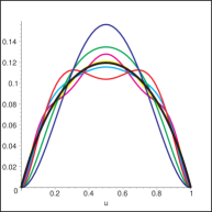
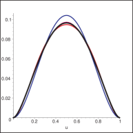
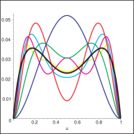
Figure 4: The first few orders (partial sums) in the conformal expansion of the renormalon model for the two–particle twist–four DA $\phi_{1}^{(4)}$ (left), $-\phi_{2}^{(4)}$ (middle) and $\phi_{1}^{(4)}+\phi_{2}^{(4)}$ (right). The thick black line represents Eq. (3).

The expansions we obtained for the three–particle DA can readily be inserted into Eq. (2.1) to yield the conformal expansions of the two–particle twist–four amplitudes. In the case of $\phi_{2}^{(4)}$ the integration can easily be performed with the result

$$\phi_{2}^{(4)}(u)=-4\delta^{2}\,u^{2}(1-u)^{2}\sum_{J=3,5,7,\ldots}^{\infty}\frac{2J-1}{J(J-1)^{2}(J-2)}\,P_{J-3}^{(2,2)}(2u-1).$$ (4.28)

Away from the end–points one can use the asymptotic expansion [35]

$$P_{n}^{(\alpha,\beta)}(\cos\theta)=\frac{\cos\{[n+(\alpha+\beta+1)/2]\theta-(2\alpha+1)\pi/4\}}{\sqrt{\pi n}\,[\sin(\theta/2)]^{\alpha+1/2}[\cos(\theta/2)]^{\beta+1/2}}+{\cal O}(n^{-3/2})$$ (4.29)

to see that Eq. (4.28) is convergent. It is not converging uniformly at the end points, however, which explains the logarithmic enhancement compared to the asymptotic DA (and the model of [6]). As noted in [6], the second derivative $(d^{2}/du^{2})\phi_{2}^{(4)}(u)$ corresponds to the non-local light–cone operator $\bar{d}(-z)\gamma^{-}\gamma_{5}\,u(z)=\bar{d}_{-}(-z)\gamma^{-}\gamma_{5}\,u_{-}(z)$ with both quarks having spin projection $s=-1/2$ alias $j_{\bar{d}}=j_{u}=1/2$. It follows that the conformal expansion of $(d^{2}/du^{2})\phi_{2}^{(4)}(u)$ goes over Legendre polynomials, or $P^{(0,0)}_{J-1}(2u-1)$. This result is consistent with Eq. (4.28) since

$$\frac{d^{2}}{du^{2}}\,\left[u^{2}(1-u)^{2}P_{J-3}^{(2,2)}(2u-1)\right]=(J-2)(J-1)\,P_{J-1}^{(0,0)}(2u-1)\,.$$ (4.30)

For $\phi_{1}^{(4)}$ a similar, closed–form all–order expression is not available. However, it is straightforward to compute the conformal expansion order by order in $J$, cf. Eq. (1):

$$\phi_{1}^{(4)}(u) = \delta^{2}\,\bigg{\{}\frac{5}{2}\bigg{[}\,u^{2}\,\bar{u}^{2}\bigg{]}_{J=3}+\frac{7}{24}\bigg{[}u\bar{u}\,(13\,u\bar{u}+2)$$ (4.31)

$$+ 2\,(6\,u^{2}+3\,u+1)\,\bar{u}^{3}\,\mathrm{ln}(\bar{u})+2\,(6\,\bar{u}^{2}+3\,\bar{u}+1)\,\,u^{3}\mathrm{ln}(u)\bigg{]}_{J=4}$$

$$+ \bigg{[}{\frac{1}{40}{u\bar{u}\,({140\,u^{2}\bar{u}^{2}+243\,u\bar{u}+42})}}+\frac{21}{20}\,(6\,u^{2}+3\,u+1)\,\bar{u}^{3}\,\mathrm{ln}(\bar{u})$$

$${}+{\frac{21}{20}}\,(6\,\bar{u}^{2}+3\,\bar{u}+1)\,u^{3}\,\mathrm{ln}(u)\bigg{]}_{J=5}+\cdots\bigg{\}}.$$

   

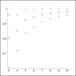
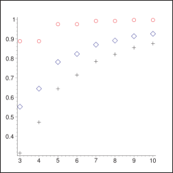
Figure 5: Subsequent approximations by the conformal expansion truncated at spin $J_{\rm max}=3,4,\ldots$ for the integrals $I_{0}$ (left panel) and $I_{1}$ (right panel) defined in Eq. (4.3.2) for $\phi_{1}^{(4)}(u)$ (diamonds), $\phi_{2}^{(4)}(u)$ (circles) and $\phi_{1}^{(4)}(u)+\phi_{2}^{(4)}(u)$ (crosses). The results are all normalized to the exact value obtained using Eq. (3). Note the different scales on the vertical axis.

Note that each term in the conformal expansion is of the order of $u^{2}(1-u)^{2}$ near the end–points but the expansion is not converging uniformly so that the $\sim u(1-u)$ behavior emerges in the sum of all spins.

The first few orders (partial sums) in the conformal expansion of the renormalon model are compared to the full result in Fig. 4 for the three functions: $\phi_{1}^{(4)}$, $\phi_{2}^{(4)}$ and $\phi_{1}^{(4)}+\phi_{2}^{(4)}$. The convergence is worst for the latter because of partial cancellation of the leading terms. Absence of uniform convergence at the end points means that the limit $u\to 0,1$ and the summation over conformal spins cannot be interchanged; the partial sums $\sum_{J=3}^{J_{\rm max}}$ diverge as $\phi_{1}^{(4)}(u)\sim(\delta^{2}/2)u^{2}(1-u)^{2}J_{\rm max}^{2}$ and $\phi_{2}^{(4)}(u)\sim-2\delta^{2}u^{2}(1-u)^{2}\ln J_{\rm max}$, respectively.

Last but not least, we show in Fig. 5 the subsequent approximations by the conformal expansion truncated at spin $J_{\rm max}=3,4,\ldots$ for the typical integrals that one encounters in the description of hard exclusive processes in QCD:

$$I_{0} = \int_{0}^{1}\frac{du}{u}\,\phi^{(4)}_{i}(u)\,,$$

$$I_{1} = \int_{0}^{1}\frac{du}{u}\ln(1/u)\,\phi^{(4)}_{i}(u)\,.$$ (4.32)

The difference between the renormalon model and the model of [6] ($J_{\rm max}=4$) is of order 10-30% for the first integral and somewhat larger for the second one.

5 Renormalon model for twist–four DA of the rho

A useful feature of the renormalon approach is its universality: with minor modifications it can be applied to DA of vector mesons as well. For definiteness we consider here $\rho^{+}$ meson. One difference to the pion case is that because of spin the number of DA proliferates significantly. We will conform to the definitions and notations of Ref. [12] and in particular distinguish between chiral–even and chiral–odd DA corresponding to the operators with odd/even number of $\gamma$–matrices, respectively, between the quark fields. A second difference is that because of a sizable $\rho$–meson mass the twist–four $\rho$–meson DA receive the Wandzura–Wilczek–type contributions of the operators with geometric twist–two given in terms of the leading–twist $\rho$–meson DA with the same (longitudinal or transverse) polarization, and the operators of geometric twist–three that are expressed in terms of twist–three DA with the opposite polarization . The Wandzura–Wilczek contributions to the vector–meson DA have been calculated in Refs. [11, 12]. They have to be added to the “genuine” twist–four contributions considered here. In this section we collect the necessary definitions and summarize the results; see Appendix C for more details.

In what follows $P_{\mu}$ stands for the $\rho$–meson momentum, $P^{2}=m_{\rho}^{2}$, and $e_{\mu}^{(\lambda)}$ is the polarization vector $e\cdot P=0$. We use the notation

$$p_{\mu}=P_{\mu}-\frac{m_{\rho}^{2}}{2p\cdot z}z_{\mu},\qquad p^{2}=0,$$

and define the transverse polarization vector by

$$e^{\perp}_{\mu}=e_{\mu}-\frac{e\cdot z}{p\cdot z}\left(p_{\mu}-\frac{m_{\rho}^{2}}{2p\cdot z}z_{\mu}\right).$$

We will also use the projector onto the directions orthogonal to $p$ and $z$:

$$g_{\mu\nu}^{\perp}=g_{\mu\nu}-\frac{1}{pz}(p_{\mu}z_{\nu}+p_{\nu}z_{\mu})\,.$$

5.1 Chiral–even distribution amplitudes

5.1.1 Definitions

We start by quoting the necessary definitions from Ref. [12] and in this section consider matrix elements involving an odd number of $\gamma$ matrices, which we refer to as chiral-even in what follows. For the vector operator the light–cone expansion to twist–four accuracy reads:

$$\langle 0|\Big{[}\bar{d}(-x)\gamma_{\mu}u(x)\Big{]}_{\mu_{F}^{2}}|\rho^{+}(P,\lambda)\rangle = f_{\rho}m_{\rho}\Bigg{\{}\frac{e^{(\lambda)}x}{Px}\,P_{\mu}\int_{0}^{1}du\,e^{-i\xi Px}\Big{[}\phi_{\parallel}(u)+\frac{m^{2}_{\rho}x^{2}}{4}\,{\mathbb{A}}(u)\Big{]}$$ (5.1)

$${}+\left(e^{(\lambda)}_{\mu}-P_{\mu}\frac{e^{(\lambda)}x}{Px}\right)\int_{0}^{1}du\,e^{-i\xi Px}\,{\mathbb{B}}(u)$$

$${}-\frac{1}{2}x_{\mu}\frac{e^{(\lambda)}x}{(Px)^{2}}m^{2}_{\rho}\int_{0}^{1}du\,e^{-i\xi Px}\,{\mathbb{C}}(u)\Bigg{\}}.$$

We do not consider the axial–vector operator because its light–cone expansion only includes contributions of twist three, five, etc., that are not relevant in the present context. For brevity, in this section we do not show gauge factors between the quark and the antiquark fields; we also use the short-hand notation

$$\xi=2u-1.$$

The vector decay constant $f_{\rho}$ is defined, as usual, as

$$\langle 0|\bar{d}(0)\gamma_{\mu}u(0)|\rho^{+}(P,\lambda)\rangle=f_{\rho}m_{\rho}e^{(\lambda)}_{\mu}\,.$$ (5.2)

The expansion in (5.1) involves three Lorentz invariant amplitudes which we have to interpret in terms of meson DA. Definitions of the latter involve non-local operators at strictly light–like separations and can most conveniently be written for longitudinal and transverse meson polarizations separately. Following [11, 12], we define chiral–even two–particle DA of the $\rho^{+}$ meson as

$$\langle 0|\Big{[}\bar{d}(-z)\gamma_{\mu}u(z)\Big{]}_{\mu_{F}^{2}}|\rho^{+}(P,\lambda)\rangle=f_{\rho}m_{\rho}\left[p_{\mu}\frac{e^{(\lambda)}z}{pz}\int_{0}^{1}\!du\,e^{-i\xi pz}\phi_{\parallel}(u,\mu_{F}^{2})\right.$$ (5.3)

$$+ \left.e^{(\lambda)}_{\perp\mu}\int_{0}^{1}\!du\,e^{-i\xi pz}g_{\perp}^{(v)}(u,\mu_{F}^{2})-\frac{1}{2}z_{\mu}\frac{e^{(\lambda)}z}{(pz)^{2}}m_{\rho}^{2}\int_{0}^{1}\!du\,e^{-i\xi pz}g_{3}(u,\mu_{F}^{2})\right].\hskip 11.38092pt$$

The distribution amplitude $\phi_{\parallel}$ is of twist two, $g_{\perp}^{(v)}$ of twist three and $g_{3}$ of twist four. All three functions $\phi=\{\phi_{\parallel},g_{\perp}^{(v)},g_{3}\}$ are normalized as

$$\int_{0}^{1}\!du\,\phi(u)=1.$$ (5.4)

This can be checked by comparing the two sides of the defining equations in the limit $z_{\mu}\to 0$ and using the EOM.

Comparing (5.3) with the light–cone expansion in (5.1) one finds [12]

$${\mathbb{B}}(u) = g^{(v)}_{\perp}(u),$$

$${\mathbb{C}}(u) = g_{3}(u)+\phi_{\parallel}(u)-2g^{(v)}_{\perp}(u)\,.$$ (5.5)

The remaining invariant amplitude ${\mathbb{A}}(u)$ accounts for the transverse momentum distribution in the valence component of the wave function. We end up with two two–particle twist–four DA of the longitudinally polarized $\rho$–meson, ${\mathbb{A}}(u)$ and $g_{3}(u)$ which are counterparts of the pion DA $\phi_{1}$ and $\phi_{2}$ (a precise correspondence will be given below).

Three–particle chiral–even distributions are rather numerous and can be defined by the following matrix elements:

$$\langle 0|\bar{d}(-z)g\widetilde{G}_{\mu\nu}(vz)\gamma_{\alpha}\gamma_{5}u(z)|\rho^{+}(P,\lambda)\rangle = f_{\rho}m_{\rho}p_{\alpha}[p_{\nu}e^{(\lambda)}_{\perp\mu}-p_{\mu}e^{(\lambda)}_{\perp\nu}]{\cal A}(v,pz)$$ (5.6)

$${}+f_{\rho}m_{\rho}^{3}\frac{e^{(\lambda)}z}{pz}[p_{\mu}g^{\perp}_{\alpha\nu}-p_{\nu}g^{\perp}_{\alpha\mu}]\widetilde{\Phi}(v,pz)$$

$${}+f_{\rho}m_{\rho}^{3}\frac{e^{(\lambda)}z}{(pz)^{2}}p_{\alpha}[p_{\mu}z_{\nu}-p_{\nu}z_{\mu}]\widetilde{\Psi}(v,pz),$$

$$\langle 0|\bar{d}(-z)gG_{\mu\nu}(vz)i\gamma_{\alpha}u(z)|\rho^{+}(P,\lambda)\rangle = f_{\rho}m_{\rho}p_{\alpha}[p_{\nu}e^{(\lambda)}_{\perp\mu}-p_{\mu}e^{(\lambda)}_{\perp\nu}]{\cal V}(v,pz)$$ (5.7)

$${}+f_{\rho}m_{\rho}^{3}\frac{e^{(\lambda)}z}{pz}[p_{\mu}g^{\perp}_{\alpha\nu}-p_{\nu}g^{\perp}_{\alpha\mu}]\Phi(v,pz)$$

$${}+f_{\rho}m_{\rho}^{3}\frac{e^{(\lambda)}z}{(pz)^{2}}p_{\alpha}[p_{\mu}z_{\nu}-p_{\nu}z_{\mu}]\Psi(v,pz),$$

where

$${\cal A}(v,pz)=\int{\cal D}{\alpha_{i}}e^{-ipz(\alpha_{u}-\alpha_{d}+v\alpha_{g})}{\cal A}(\alpha_{i}),$$ (5.8)

etc., and ${\alpha_{i}}$ is the set of three momentum fractions $\{\alpha_{1},\alpha_{2},\alpha_{3}\}=\{\alpha_{u},\alpha_{d},\alpha_{g}\}$. The integration measure is defined in Eq. (2.11).

Similarly to the pion case, all higher–twist two–particle DA of the $\rho$–meson do not present genuine independent degrees of freedom but can be expressed in terms of three–particle DA. The corresponding relations [12] are given in Eq. (C.1) below.

In addition, we introduce a new twist–four DA

$$\left\langle 0\left|\bar{d}(-z)\gamma_{\mu}gD^{\alpha}G_{\alpha\beta}(vz)u(z)\right|\rho^{+}(P,\lambda)\right\rangle=f_{\rho}m_{\rho}^{3}\,p_{\mu}p_{\beta}\,\frac{e^{(\lambda)}z}{pz}\Xi_{\rho}(v,pz)\,,$$ (5.9)

which can be viewed, equivalently, either as a three–particle quark–antiquark–gluon DA, or as a special case of a four-quark DA with the quark-antiquark pair in a color–octet state and at the same space point, cf. Eq. (2.1).

5.1.2 Renormalon model and comparison with Ref. [12]

The renormalon model for twist–four DA of the longitudinally polarized $\rho$–meson can most simply be derived from the UV–renormalon ambiguity in twist–four operators. The calculation is very similar to that in the pion case. One obtains in the single–dressed–gluon approximation

$$\delta_{\hbox{\tiny UV}}\Big{\{}z^{\mu}\,\bar{d}(-z)\gamma^{\nu}\gamma_{5}g\widetilde{G}_{\mu\nu}(vz)u(z)\Big{\}} = 2\,c\Lambda^{2}\,\int_{0}^{1}da(1+a)\,\bigg{[}\bar{d}(-y)\mbox{$z$\raisebox{0.43057pt}{$/$}}u(z)+\bar{d}(-z)\mbox{$z$\raisebox{0.43057pt}{$/$}}u(\widetilde{y})\bigg{]},$$

$$\delta_{\hbox{\tiny UV}}\Big{\{}z^{\mu}\,\bar{d}(-z)\mbox{$z$\raisebox{0.43057pt}{$/$}}\gamma_{5}g\widetilde{G}_{\mu\rho}(vz)u(z)\Big{\}} = 2\,c\Lambda^{2}\,z_{\rho}\,\int_{0}^{1}da\,a\,\bigg{[}\bar{d}(-y)\mbox{$z$\raisebox{0.43057pt}{$/$}}u(z)+\bar{d}(-z)\mbox{$z$\raisebox{0.43057pt}{$/$}}u(\widetilde{y})\bigg{]},$$

$$\delta_{\hbox{\tiny UV}}\Big{\{}z^{\mu}\,\bar{d}(-z)\gamma^{\nu}igG_{\mu\nu}(vz)u(z)\Big{\}} = -2\,c\Lambda^{2}\,\int_{0}^{1}da(1-a)\,\bigg{[}\bar{d}(-y)\mbox{$z$\raisebox{0.43057pt}{$/$}}u(z)-\bar{d}(-z)\mbox{$z$\raisebox{0.43057pt}{$/$}}u(\widetilde{y})\bigg{]},$$

$$\delta_{\hbox{\tiny UV}}\Big{\{}z^{\mu}\,\bar{d}(-z)\mbox{$z$\raisebox{0.43057pt}{$/$}}igG_{\mu\rho}(vz)u(z)\Big{\}} = 2\,c\Lambda^{2}\,z_{\rho}\,\int_{0}^{1}da\,a\,\bigg{[}\bar{d}(-y)\mbox{$z$\raisebox{0.43057pt}{$/$}}u(z)-\bar{d}(-z)\mbox{$z$\raisebox{0.43057pt}{$/$}}u(\widetilde{y})\bigg{]},$$

$$\delta_{\hbox{\tiny UV}}\Big{\{}z^{\beta}\bar{d}(-z)gD^{\alpha}G_{\alpha\beta}(vz)\mbox{$z$\raisebox{0.43057pt}{$/$}}u(z)\Big{\}} = -4ic\Lambda^{2}\int_{0}^{1}da\,a\frac{d}{da}\bigg{[}\frac{1}{1+v}\,\bar{d}(-y)\mbox{$z$\raisebox{0.43057pt}{$/$}}u(z)$$ (5.10)

$$\hskip 83.0pt+\,\frac{1}{1-v}\bar{d}(-z)\mbox{$z$\raisebox{0.43057pt}{$/$}}u(\widetilde{y})\bigg{]},$$

where $c$ is given in Eq. (2.33) and the variables $y$ and $\widetilde{y}$ are defined below Eq. (2.3). To obtain the renormalon model, we take the matrix elements of the operators in Eq. (5.1.2) between the vacuum and a $\rho$–meson state, project onto the relevant Lorentz structures and fix the normalization by the local matrix element

$$\langle 0|\bar{d}(0)g\widetilde{G}_{\mu\nu}(0)\gamma^{\nu}\gamma_{5}u(0)|\rho^{+}(P,\lambda)\rangle=f_{\rho}m_{\rho}^{3}e^{(\lambda)}_{\mu}\zeta_{4}\,,~{}~{}~{}\zeta_{4}=0.15\pm 0.10~{}\mbox{\cite[cite]{[\@@bibref{}{BK85}{}{}]}}$$ (5.11)

making the substitution

$$c\Lambda^{2}\to\frac{1}{6}\zeta_{4}\,m^{2}_{\rho}\,.$$ (5.12)

The resulting twist–four DA, expressed in terms of the twist–two one, read:

$$\widetilde{\Psi}(\alpha_{i}) = \frac{1}{3}\zeta_{4}\left[\frac{\alpha_{2}\phi_{\parallel}(\alpha_{1})}{(1-\alpha_{1})^{2}}+\frac{\alpha_{1}\phi_{\parallel}(\alpha_{2})}{(1-\alpha_{2})^{2}}\right],$$

$$\Psi(\alpha_{i})\Big{\}} = \frac{1}{3}\zeta_{4}\left[\frac{\alpha_{2}\phi_{\parallel}(\alpha_{1})}{(1-\alpha_{1})^{2}}-\frac{\alpha_{1}\phi_{\parallel}(\alpha_{2})}{(1-\alpha_{2})^{2}}\right],$$

$$\widetilde{\Phi}(\alpha_{i}) = \frac{1}{6}\zeta_{4}\left[\frac{\phi_{\parallel}(\alpha_{1})}{1-\alpha_{1}}+\frac{\phi_{\parallel}(\alpha_{2})}{1-\alpha_{2}}\right],$$

$$\Phi(\alpha_{i}) = -\frac{1}{6}\zeta_{4}\left[\frac{\phi_{\parallel}(\alpha_{1})}{1-\alpha_{1}}-\frac{\phi_{\parallel}(\alpha_{2})}{1-\alpha_{2}}\right],$$

$$\Xi_{\rho}(\alpha_{i}) = -\frac{2}{3}\zeta_{4}\left[\frac{\alpha_{2}}{1-\alpha_{1}}\,\phi_{\parallel}(\alpha_{1})-\frac{\alpha_{1}}{1-\alpha_{2}}\phi_{\parallel}(\alpha_{2})\right],$$ (5.13)

where we used the symmetry $\phi_{\parallel}(u)=\phi_{\parallel}(1-u)$. Note the similarity of this result to the pion case, Eq. (3): upon replacing in the latter $\delta^{2}$ by $\zeta_{4}$ one recovers the former with $-\Phi_{\perp}^{\pi}\longrightarrow\Phi^{\rho},\,\Phi_{\parallel}^{\pi}\longrightarrow\Psi^{\rho},\,\Psi_{\perp}^{\pi}\longrightarrow\widetilde{\Phi}^{\rho},\,-\Psi_{\parallel}^{\pi}\longrightarrow\widetilde{\Psi}^{\rho}$ and $\Xi_{\pi}\longrightarrow\Xi_{\rho}$.

The two–particle twist–four DA can now be restored using EOM [12]. The calculation (see Appendix C.1) gives:

$$\mathbb{A}(u) = \frac{8}{3}\zeta_{4}\int_{0}^{1}dv\,\phi_{\parallel}(v)\bigg{\{}\theta(u>v)\;\frac{1}{\bar{v}^{2}}\left[{\bar{u}+\bar{u}^{2}+(u-v)\ln\frac{u-v}{\bar{v}}}\right]$$

$$\hskip 93.0pt+\theta(u<v)\;\frac{1}{v^{2}}\left[{u+u^{2}+(v-u)\ln\frac{v-u}{v}}\right]\bigg{\}},$$

$$g_{3}(u) = -\frac{2}{3}\zeta_{4}\left\{\int_{0}^{1}\!dv\,\phi_{\parallel}(v)\left[\theta(u>v)\;\frac{1}{\bar{v}^{2}}+\theta(u<v)\;\frac{1}{v^{2}}\right]-\frac{\phi_{\parallel}(u)}{u\bar{u}}\right\}.$$ (5.14)

Continuing the comparison with the pion case $\mathbb{A}(u)$ is similar to $16(\phi_{1}-\phi_{2})$ and $g_{3}$ to $2{d^{2}\phi_{2}}/{du^{2}}$.

Eqs. (5.1.2) and (5.1.2) are valid for an arbitrary leading–twist DA. Choosing the asymptotic expression $\phi_{\parallel}(u)=6u(1-u)$ yields a simple model

$$\widetilde{\Psi}(\alpha_{i}) = 2\zeta_{4}\alpha_{1}\alpha_{2}\left[\frac{1}{1-\alpha_{1}}+\frac{1}{1-\alpha_{2}}\right],$$

$${\Psi}(\alpha_{i}) = 2\zeta_{4}\alpha_{1}\alpha_{2}\left[\frac{1}{1-\alpha_{1}}+\frac{1}{1-\alpha_{2}}\right],$$

$$\widetilde{\Phi}(\alpha_{i}) = \zeta_{4}\left[\alpha_{1}+\alpha_{2}\right],$$

$$\Phi(\alpha_{i}) = \zeta_{4}[\alpha_{2}-\alpha_{1}],$$

$$\Xi_{\rho}(\alpha_{i}) = 0$$ (5.15)

and

$$\mathbb{A}(u) = 16\zeta_{4}\bigg{\{}\bar{u}\bigg{[}u\ln(\bar{u})-\mbox{\rm Li}_{2}(\bar{u})\bigg{]}+u\bigg{[}\bar{u}\ln(u)-\mbox{\rm Li}_{2}(u)\bigg{]}-2u\bar{u}+\frac{\pi^{2}}{6}\bigg{\}},$$

$$g_{3}(u) = 4\zeta_{4}\bigg{\{}\ln(u)+\ln(\bar{u})+2\bigg{\}}.$$ (5.16)

This model should be compared with that of Ball and Braun (BB) in Ref. [12] based on the two first orders in the conformal expansion:

$$\widetilde{\Psi}^{\rm BB}(\alpha_{i}) = 40\,\zeta_{4}\,\alpha_{1}\alpha_{2}\alpha_{3}\Big{[}1+\frac{63}{4}\omega_{4}^{A}(3\alpha_{3}-1)\Big{]},$$

$$\Psi^{\rm BB}(\alpha_{i}) = 630\,\zeta_{4}\,\omega_{4}^{A}\,\alpha_{1}\alpha_{2}\alpha_{3}(\alpha_{2}-\alpha_{1})\,,$$

$$\widetilde{\Phi}^{\rm BB}(\alpha_{i}) = 10\,\zeta_{4}\,\alpha_{3}^{2}(1-\alpha_{3})\Big{[}1+\frac{63}{2}\omega_{4}^{A}(2\alpha_{3}-1)\Big{]},$$

$$\Phi^{\rm BB}(\alpha_{i}) = 10\,\zeta_{4}\,\alpha_{3}^{2}(\alpha_{2}-\alpha_{1})\Big{[}1+\frac{63}{2}\omega_{4}^{A}(2\alpha_{3}-1)\Big{]},$$

$$\Xi_{\rho}^{\rm BB}(\alpha_{i}) = 0\,,$$ (5.17)

where the new parameter $\omega_{4}^{A}$ is defined by the matrix element of the $J=4$ local operator in Eq. (4.21) in Ref. [12]. From QCD sum rules [12] one obtains a crude estimate:

$$\left.\omega_{4}^{A}\right|_{\rm SR}=0.8\pm 0.8\,.$$ (5.18)

To the same $J=4$ accuracy

$$\mathbb{A}^{\rm BB}(u) = \frac{200}{3}\zeta_{4}u^{2}\bar{u}^{2}-42\zeta_{4}\omega_{4}^{A}\Big{\{}u\bar{u}(2+13u\bar{u})+2u^{3}(1+3\bar{u}+6\bar{u}^{2})\ln u$$

$${}+2\bar{u}^{3}(1+3u+6u^{2})\ln\bar{u}\Big{\}},$$

$$g_{3}^{\rm BB}(u) = -\frac{20}{3}\zeta_{4}(1-6u\bar{u})\,.$$ (5.19)

To avoid misunderstanding, note that for this comparison we suppressed the Wandzura–Wilczek contributions of twist–two and twist–three operators to the coefficients in the conformal expansion in [12] and only retained the genuine twist–four contributions.

Performing the conformal expansion of the renormalon model, Eq. (5.1.2), up to $J=4$ we recover the structure of Eq. (5.1.2) predicting:

$$\left.\omega_{4}^{A}\right|_{\rm Ren}=-\frac{1}{9},$$ (5.20)

which can be contrasted with the sum–rule result in Eq. (5.18). Similar to the pion case, this number is not sensitive to the shape of the leading–twist DA.

Figure 6 compares the renormalon model with that of Ref. [12]. For $g_{3}(u)$ the main difference is in the asymptotic end–point behavior: it is logarithmic in the renormalon model and constant in the model of Ref. [12]. For $\mathbb{A}(u)$ the difference is more pronounced — the asymptotic behavior is linear and quadratic in the two models, respectively — and, moreover, it extends to the central region because of the very different $J=4$ contributions which are determined by Eq. (5.20) and the central value of Eq. (5.18), respectively. Figure 7 makes a similar comparison but this time adding the Wandzura–Wilczek terms in both models.

      

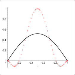
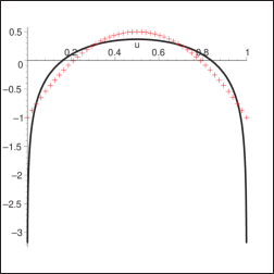
Figure 6: The two–particle twist–four DA of the $\rho$ in the chiral–even sector, $\mathbb{A}(u)$ (left) and $g_{3}(u)$ (right) based on the renormalon model of Eq. (5.1.2) (full line) and model of Ref. [12], given by Eq. (5.1.2) (crosses), which uses the first two orders in the conformal expansion with the sum–rule estimate $\omega_{4}^{A}=0.8$. The normalization is chosen to be the same $\zeta_{4}=0.15$.

      

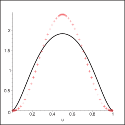
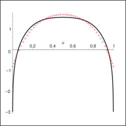
Figure 7: The same as Fig. 6, but including (in both models) the Wandzura–Wilczek contributions as given by Eqs. (4.22) and (4.23) in Ref. [12] with the parameters of Table 2 there, except that we consistently use the asymptotic leading–twist DA, so $a_{2}^{\parallel}=0$.

5.2 Chiral–odd distribution amplitudes

5.2.1 Definitions

For the chiral-odd operator involving the $\sigma_{\mu\nu}$–matrix the light–cone expansion to twist–four accuracy reads [12]:

$$\langle 0|\Big{[}\bar{d}(-x)\sigma_{\mu\nu}u(x)\Big{]}_{\mu_{F}^{2}}\!|\rho^{+}\!(P,\lambda)\rangle = if_{\rho}^{T}\!\left\{(e^{(\lambda)}_{\mu}\!P_{\nu}-e^{(\lambda)}_{\nu}\!P_{\mu})\!\!\int_{0}^{1}\!\!\!\!du\,e^{-i\xi Px}\bigg{[}\phi_{\perp}(u)+\frac{m_{\rho}^{2}x^{2}}{4}{\mathbb{A}}_{T}(u)\bigg{]}\right.$$ (5.21)

$${}+(P_{\mu}x_{\nu}-P_{\nu}x_{\mu})\frac{e^{(\lambda)}x}{(Px)^{2}}m_{\rho}^{2}\int_{0}^{1}\!du\,e^{-i\xi Px}{\mathbb{B}}_{T}(u)$$

$$\left.{}+\frac{1}{2}(e^{(\lambda)}_{\mu}x_{\nu}-e^{(\lambda)}_{\nu}x_{\mu})\frac{m_{\rho}^{2}}{Px}\int_{0}^{1}\!du\,e^{-i\xi Px}{\mathbb{C}}_{T}(u)\right\},$$

where the tensor coupling $f_{\rho}^{T}$ is given by

$$\langle 0|\bar{u}(0)\sigma_{\mu\nu}d(0)|\rho^{-}(P,\lambda)\rangle=if_{\rho}^{T}(e_{\mu}^{(\lambda)}P_{\nu}-e_{\nu}^{(\lambda)}P_{\mu}).$$ (5.22)

In comparison, the corresponding light–cone DA are defined as

$$\langle 0|\Big{[}\bar{d}(-z)\sigma_{\mu\nu}u(z)\Big{]}_{\mu_{F}^{2}}\!|\rho^{+}\!(P,\lambda)\rangle = if_{\rho}^{T}\bigg{\{}(e^{(\lambda)}_{\perp\mu}p_{\nu}-e^{(\lambda)}_{\perp\nu}p_{\mu})\int_{0}^{1}\!du\,e^{-i\xi pz}\phi_{\perp}(u,\mu_{F}^{2})$$ (5.23)

$$+(p_{\mu}z_{\nu}-p_{\nu}z_{\mu})\frac{e^{(\lambda)}z}{(pz)^{2}}m_{\rho}^{2}\int_{0}^{1}\!du\,e^{-i\xi pz}h_{\parallel}^{(t)}(u,\mu_{F}^{2})$$

$$+\frac{1}{2}(e^{(\lambda)}_{\perp\mu}z_{\nu}-e^{(\lambda)}_{\perp\nu}z_{\mu})\frac{m_{\rho}^{2}}{pz}\!\int_{0}^{1}\!\!du\,e^{-i\xi pz}h_{3}(u,\mu_{F}^{2})\bigg{\}},$$

where $\phi_{\perp}(u)$ is the leading–twist DA of the transversely polarized $\rho$–meson, $h_{\parallel}^{(t)}(u)$ is of twist–three and of no interest for our present purposes, and $h_{3}(u)$ is of twist–four. All three functions $\phi=\{\phi_{\perp},h_{\parallel}^{(t)},h_{3}\}$ are normalized as $\int_{0}^{1}du\,\phi(u)=1.$ Matching (5.23) with the light-cone expansion in Eq. (5.21) one obtains

$${\mathbb{B}}_{T}(u) = h_{\parallel}^{(t)}(u)-\frac{1}{2}\phi_{\perp}(u)-\frac{1}{2}h_{3}(u),$$

$${\mathbb{C}}_{T}(u) = h_{3}(u)-\phi_{\perp}(u).$$ (5.24)

The remaining invariant amplitude ${\mathbb{A}}_{T}(u)$ describes the transverse momentum distribution in the leading–twist component of the wave function. We end up with two two–particle twist–four DA of the transversely polarized $\rho$–meson, ${\mathbb{A}}_{T}(u)$ and $h_{3}(u)$ which are counterparts of the distributions ${\mathbb{A}}(u)$ and $g_{3}(u)$ for the longitudinally polarized $\rho$–meson and of the pion DA $\phi_{1}^{(4)}(u)$ and $\phi_{2}^{(4)}(u)$ defined in Eq. (2.1). The precise correspondence will be given below.

The three–particle DA are even more numerous than in the chiral-even case and can be defined as [12]:

$$\langle 0|\bar{d}(-z)\sigma_{\alpha\beta}gG_{\mu\nu}(vz)u(z)|\rho^{+}(P,\lambda)\rangle\ =$$ (5.25)

$$= f_{\rho}^{T}m_{\rho}^{2}\frac{e^{(\lambda)}z}{2(pz)}\bigg{[}p_{\alpha}p_{\mu}g^{\perp}_{\beta\nu}-p_{\beta}p_{\mu}g^{\perp}_{\alpha\nu}-p_{\alpha}p_{\nu}g^{\perp}_{\beta\mu}+p_{\beta}p_{\nu}g^{\perp}_{\alpha\mu}\bigg{]}{\cal T}(v,pz)$$

$$+ f_{\rho}^{T}m_{\rho}^{2}\bigg{[}p_{\alpha}e^{(\lambda)}_{\perp\mu}g^{\perp}_{\beta\nu}-p_{\beta}e^{(\lambda)}_{\perp\mu}g^{\perp}_{\alpha\nu}-p_{\alpha}e^{(\lambda)}_{\perp\nu}g^{\perp}_{\beta\mu}+p_{\beta}e^{(\lambda)}_{\perp\nu}g^{\perp}_{\alpha\mu}\bigg{]}T_{1}(v,pz)$$

$$+ f_{\rho}^{T}m_{\rho}^{2}\bigg{[}p_{\mu}e^{(\lambda)}_{\perp\alpha}g^{\perp}_{\beta\nu}-p_{\mu}e^{(\lambda)}_{\perp\beta}g^{\perp}_{\alpha\nu}-p_{\nu}e^{(\lambda)}_{\perp\alpha}g^{\perp}_{\beta\mu}+p_{\nu}e^{(\lambda)}_{\perp\beta}g^{\perp}_{\alpha\mu}\bigg{]}T_{2}(v,pz)$$

$$+ \frac{f_{\rho}^{T}m_{\rho}^{2}}{pz}\bigg{[}p_{\alpha}p_{\mu}e^{(\lambda)}_{\perp\beta}z_{\nu}-p_{\beta}p_{\mu}e^{(\lambda)}_{\perp\alpha}z_{\nu}-p_{\alpha}p_{\nu}e^{(\lambda)}_{\perp\beta}z_{\mu}+p_{\beta}p_{\nu}e^{(\lambda)}_{\perp\alpha}z_{\mu}\bigg{]}T_{3}(v,pz)$$

$$+ \frac{f_{\rho}^{T}m_{\rho}^{2}}{pz}\bigg{[}p_{\alpha}p_{\mu}e^{(\lambda)}_{\perp\nu}z_{\beta}-p_{\beta}p_{\mu}e^{(\lambda)}_{\perp\nu}z_{\alpha}-p_{\alpha}p_{\nu}e^{(\lambda)}_{\perp\mu}z_{\beta}+p_{\beta}p_{\nu}e^{(\lambda)}_{\perp\mu}z_{\alpha}\bigg{]}T_{4}(v,pz),\hskip 28.45274pt$$

$$\langle 0|\bar{d}(-z)gG_{\mu\nu}(vz)u(z)|\rho^{+}(P,\lambda)\rangle\ =\ if_{\rho}^{T}m_{\rho}^{2}\bigg{[}e^{(\lambda)}_{\perp\mu}p_{\nu}-e^{(\lambda)}_{\perp\nu}p_{\mu}\bigg{]}S(v,pz),$$

$$\langle 0|\bar{d}(-z)ig\widetilde{G}_{\mu\nu}(vz)\gamma_{5}u(z)|\rho^{+}(P,\lambda)\rangle\ =\ if_{\rho}^{T}m_{\rho}^{2}\bigg{[}e^{(\lambda)}_{\perp\mu}p_{\nu}-e^{(\lambda)}_{\perp\nu}p_{\mu}\bigg{]}\widetilde{S}(v,pz).$$ (5.26)

Of these seven amplitudes ${\cal T}$ is of twist three and the other six of twist four; higher–twist terms are suppressed.

We also introduce one more twist–four DA as follows

$$\langle 0|\bar{d}(-z)\sigma_{\mu\nu}gD^{\alpha}G_{\alpha\beta}(vz)u(z)|\rho^{+}(P,\lambda)\rangle=if_{\rho}m_{\rho}^{2}\,\bigg{[}e^{(\lambda)}_{\perp\mu}p_{\nu}-e^{(\lambda)}_{\perp\nu}p_{\mu}\bigg{]}p_{\beta}\,\Xi^{T}_{\rho}(v,pz)\,.$$ (5.27)

As in the other cases the twist–four two–particle DA do not present independent degrees of freedom and can be expressed in terms of three–particle DA using EOM [12], see Eq. (C.1) below.

5.2.2 Renormalon model and comparison with Ref. [12]

Computing the first UV–renormalon contribution to the operator $\bar{d}(-z)\sigma_{\alpha\beta}G_{\mu\nu}(vz)u(z)$, and taking the relevant Lorentz projections we find

$$\delta_{\hbox{\tiny UV}}\Big{\{}\,\bar{d}(-z)e_{\perp\nu}^{(\lambda)}z^{\beta}\,\sigma_{\mu\beta}\,g{G}^{\mu\nu}(vz)u(z)\Big{\}}$$

$$\hskip 50.0pt=-ic\Lambda^{2}\,e_{\perp\rho}^{(\lambda)}z_{\varepsilon}\int_{0}^{1}da(1+2a)\,\bigg{[}\bar{d}(-y)\sigma^{\rho\varepsilon}u(z)-\bar{d}(-z)\sigma^{\rho\varepsilon}u(\widetilde{y})\bigg{]},$$

$$\delta_{\hbox{\tiny UV}}\Big{\{}\,\bar{d}(-z)e^{(\lambda)}_{\perp\beta}z^{\nu}\,\sigma^{\mu\beta}\,g{G}_{\mu\nu}(vz)u(z)\Big{\}}$$

$$\hskip 50.0pt=ic\Lambda^{2}\,e^{(\lambda)}_{\perp\rho}z_{\varepsilon}\,\int_{0}^{1}da\,(1-2a)\,\bigg{[}\bar{d}(-y)\sigma^{\rho\varepsilon}u(z)-\bar{d}(-z)\sigma^{\rho\varepsilon}u(\widetilde{y})\bigg{]},$$

$$\delta_{\hbox{\tiny UV}}\Big{\{}\,\bar{d}(-z)e^{(\lambda)}_{\perp\beta}z_{\alpha}z_{\mu}\,\sigma^{\alpha\beta}\,gG^{\mu\nu}(vz)u(z)\Big{\}}$$

$$\hskip 50.0pt=-2ic\Lambda^{2}\,z^{\nu}z_{\rho}e^{(\lambda)}_{\perp\varepsilon}\int_{0}^{1}da\,a\,\bigg{[}\bar{d}(-y)\sigma^{\rho\varepsilon}u(z)-\bar{d}(-z)\sigma^{\rho\varepsilon}u(\widetilde{y})\bigg{]},$$

$$\delta_{\hbox{\tiny UV}}\Big{\{}\,\bar{d}(-z)e^{(\lambda)}_{\perp\nu}z_{\alpha}z_{\mu}\,\sigma^{\alpha\beta}\,gG^{\mu\nu}(vz)u(z)\Big{\}}$$

$$\hskip 50.0pt=-ic\Lambda^{2}\,z^{\beta}z_{\rho}e^{(\lambda)}_{\perp\varepsilon}\int_{0}^{1}da\,\bigg{[}\bar{d}(-y)\sigma^{\rho\varepsilon}u(z)-\bar{d}(-z)\sigma^{\rho\varepsilon}u(\widetilde{y})\bigg{]},$$ (5.28)

where $y$ and $\widetilde{y}$ are defined below Eq. (2.3). In a similar manner, for the operators $\bar{d}(-z)G_{\alpha\beta}(vz)u(z)$ and $\bar{d}(-z)\gamma_{5}i\widetilde{G}_{\alpha\beta}(vz)u(z)$ we obtain

$$\delta_{\hbox{\tiny UV}}\Big{\{}\bar{d}(-z)e^{(\lambda)}_{\perp\nu}z^{\mu}\,gG_{\mu\nu}(vz)u(z)\Big{\}}=\,c\Lambda^{2}\,z^{\alpha}e^{(\lambda)}_{\perp\beta}\int_{0}^{1}da\bigg{[}\bar{d}(-y)\sigma_{\alpha\beta}u(z)+\bar{d}(-z)\sigma_{\alpha\beta}u(\widetilde{y})\bigg{]},$$

$$\delta_{\hbox{\tiny UV}}\Big{\{}\bar{d}(-z)e^{(\lambda)}_{\perp\nu}z^{\mu}\gamma_{5}ig\widetilde{G}_{\mu\nu}(vz)u(z)\Big{\}}=\,-c\Lambda^{2}\,z^{\alpha}e^{(\lambda)}_{\perp\beta}\int_{0}^{1}\!\!da\,\bigg{[}\bar{d}(-y)\sigma_{\alpha\beta}u(z)+\bar{d}(-z)\sigma_{\alpha\beta}u(\widetilde{y})\bigg{]},$$

and finally for the operator $\bar{d}(-z)\sigma_{\mu\nu}gD^{\alpha}G_{\alpha\beta}(vz)u(z)$ we get

$$\delta_{\hbox{\tiny UV}}\Big{\{}z^{\beta}\bar{d}(-z)gD^{\alpha}G_{\alpha\beta}(vz)\sigma_{\mu\nu}u(z)\Big{\}}$$

$$\hskip 50.0pt=-4ic\Lambda^{2}\int_{0}^{1}da\,a\frac{d}{da}\bigg{[}\frac{1}{1+v}\,\bar{d}(-y)\sigma_{\mu\nu}u(z)+\,\frac{1}{1-v}\bar{d}(-z)\sigma_{\mu\nu}u(\widetilde{y})\bigg{]}.$$ (5.30)

Taking the matrix elements of the operators in Eq. (5.2.2) through Eq. (5.2.2) between the vacuum and the $\rho$–meson state we extract the renormalon ambiguity for these twist–four DA in terms of $\phi_{\perp}(u)$. Going over from the renormalon ambiguity to a model, one has to take into account that in the present case there exist two independent local operators of the lowest dimension that have proper quantum numbers:

$$\langle 0|\bar{d}(0)gG_{\mu\nu}(0)u(0)|\rho^{+}(P,\lambda)\rangle = if_{\rho}^{T}m_{\rho}^{2}\zeta^{T}_{4}(e^{(\lambda)}_{\mu}P_{\nu}-e^{(\lambda)}_{\nu}P_{\mu}),$$

$$\langle 0|\bar{d}(0)g\widetilde{G}_{\mu\nu}(0)i\gamma_{5}u(0)|\rho^{+}(P,\lambda)\rangle = if_{\rho}^{T}m_{\rho}^{2}\widetilde{\zeta}^{T}_{4}(e^{(\lambda)}_{\mu}P_{\nu}-e^{(\lambda)}_{\nu}P_{\mu}).$$ (5.31)

The parameters $\zeta_{4}^{T}\pm\widetilde{\zeta}_{4}^{T}$ renormalize multiplicatively with different anomalous dimensions [40] and from the QCD sum rules one finds [40, 12]

$$\zeta_{4}^{T}-\widetilde{\zeta}_{4}^{T} = 0.2\pm 0.1\,,$$

$$\zeta_{4}^{T}+\widetilde{\zeta}_{4}^{T} = 0\,.$$ (5.32)

The vanishing (or smallness) of the second number in Eq. (5.2.2) appears as a consequence of vanishing of the leading contribution to the corresponding correlation function, see Appendix C in [12].

By comparison of the expressions in Eq. (5.2.2) we observe that the leading UV–renormalon contribution to the operator $\bar{d}(-z)[gG_{\mu\nu}+g\widetilde{G}_{\mu\nu}i\gamma_{5}](vz)u(z)$ and thus to $\zeta_{4}^{T}+\widetilde{\zeta}_{4}^{T}$ vanishes as well. Therefore, within the renormalon model $\widetilde{\zeta}_{4}^{T}=-\zeta_{4}^{T}$ and similarly to the pion and the chiral–even $\rho$–meson cases the model has only one parameter.

Collecting everything and making the substitution

$$c\Lambda^{2}\to\frac{1}{2}\zeta_{4}^{T}m_{\rho}^{2}$$ (5.33)

we obtain

$$T_{1}(\alpha_{i})=-T_{3}(\alpha_{i})=\zeta_{4}^{T}\left[\frac{\alpha_{2}\phi_{\perp}(\alpha_{1})}{(1-\alpha_{1})^{2}}-\frac{\alpha_{1}\phi_{\perp}(\alpha_{2})}{(1-\alpha_{2})^{2}}\right],$$

$$T_{2}(\alpha_{i})=\phantom{-}T_{4}(\alpha_{i})=-\frac{1}{2}\zeta_{4}^{T}\left[\frac{\phi_{\perp}(\alpha_{1})}{(1-\alpha_{1})}-\frac{\phi_{\perp}(\alpha_{2})}{(1-\alpha_{2})}\right],$$

$$S(\alpha_{i})=-\,\widetilde{S}(\alpha_{i})\,=\,\frac{1}{2}\zeta_{4}^{T}\left[\frac{\phi_{\perp}(\alpha_{1})}{1-\alpha_{1}}+\frac{\phi_{\perp}(\alpha_{2})}{1-\alpha_{2}}\right],$$

$$\Xi^{T}_{\rho}(\alpha_{i})=-2\zeta_{4}^{T}\left[\frac{\alpha_{2}}{1-\alpha_{1}}\,\phi_{\perp}(\alpha_{1})-\frac{\alpha_{1}}{1-\alpha_{2}}\phi_{\perp}(\alpha_{2})\right],$$ (5.34)

where we used the symmetry $\phi_{\perp}(u)=\phi_{\perp}(1-u)$. The correspondence with the pion DA is as follows: upon replacing $\delta^{2}$ by $3\zeta_{4}^{T}$, $\Phi_{\parallel}^{\pi}\longrightarrow T_{1}^{\rho}$, $\Phi_{\perp}^{\pi}\longrightarrow-T_{2}^{\rho}$, $\Psi_{\perp}^{\pi}\longrightarrow S^{\rho}$ and $\Xi_{\pi}\longrightarrow\Xi^{T}_{\rho}$. There is no analog for $\Psi_{\parallel}^{\pi}$.

Finally, the two–particle twist–four DA are restored using EOM (see Appendix C.1):

$$\mathbb{A}_{T}(u) = 8\zeta_{4}^{T}\int_{0}^{1}dv\,\phi_{\perp}(v)\Bigg{[}\theta(u>v)\;\frac{1}{\bar{v}^{2}}\left({\bar{u}+(u-v)\ln\frac{u-v}{\bar{v}}}\right)$$

$$\hskip 80.0pt+\theta(u<v)\;\frac{1}{v^{2}}\left({u+(v-u)\ln\frac{v-u}{v}}\right)\Bigg{]},$$

$$h_{3}(u) = 0\,.$$ (5.35)

Note that there is no renormalon ambiguity in $h_{3}(u)$ at the level of a single dressed gluon, and therefore in our model this DA vanishes. Also note that apart from the different overall normalization ($\delta^{2}\longrightarrow 3\zeta_{4}^{T}$) $\mathbb{A}_{T}(u)$ is the same as $16\phi^{(4)}_{1}(u)$ in the pion case.

Choosing the asymptotic leading–twist DA $\phi_{\perp}(u)=6u(1-u)$ we obtain simple expressions

$$T_{1}(\alpha_{i})=-T_{3}(\alpha_{i})=6\zeta_{4}^{T}\alpha_{1}\alpha_{2}\left[\frac{1}{1-\alpha_{1}}-\frac{1}{1-\alpha_{2}}\right]\,,$$ (5.36)

$$T_{2}(\alpha_{i})=\phantom{-}T_{4}(\alpha_{i})=3\zeta_{4}^{T}[\alpha_{2}-\alpha_{1}]\,,$$

$$S(\alpha_{i})=-\,\widetilde{S}(\alpha_{i})\,=\,3\zeta_{4}^{T}\left[\alpha_{1}+\alpha_{2}\right],$$

$$\Xi^{T}_{\rho}(\alpha_{i})=0$$

and

$$\mathbb{A}_{T}(u) = 48\zeta_{4}^{T}\bigg{\{}\bar{u}\bigg{[}\ln(\bar{u})-\mbox{\rm Li}_{2}(\bar{u})\bigg{]}+u\bigg{[}\ln(u)-\mbox{\rm Li}_{2}(u)\bigg{]}-u\bar{u}+\frac{\pi^{2}}{6}\bigg{\}},$$

$$h_{3}(u) = 0\,.$$ (5.37)

These results can be compared with the model of [12]. The structure of the conformal expansion to spin $J=4$ accuracy is more complicated in this case as it involves three parameters. Following [12] we write

$$T_{1}({\alpha_{i}}) = \phantom{-}120t_{10}(\alpha_{2}-\alpha_{1})\alpha_{2}\alpha_{1}\alpha_{3},$$

$$T_{2}({\alpha_{i}}) = -30\alpha_{3}^{2}(\alpha_{2}-\alpha_{1})\left[\widetilde{s}_{00}+\frac{1}{2}\,\widetilde{s}_{10}\,(5\alpha_{3}-3)+\widetilde{s}_{01}\alpha_{3}\right],$$

$$T_{3}({\alpha_{i}}) = -120\widetilde{t}_{10}(\alpha_{2}-\alpha_{1})\alpha_{2}\alpha_{1}\alpha_{3},$$

$$T_{4}({\alpha_{i}}) = \phantom{-}30\alpha_{3}^{2}(\alpha_{2}-\alpha_{1})\left[s_{00}+\frac{1}{2}\,s_{10}\,(5\alpha_{3}-3)+s_{01}\alpha_{3}\right],$$ (5.38)

$${S}({\alpha_{i}}) = 30\alpha_{3}^{2}\!\left[s_{00}\,(1\!-\!\alpha_{3})+s_{10}\left\{\!\alpha_{3}(1\!-\!\alpha_{3})-\frac{3}{2}\,(\alpha_{2}^{2}+\alpha_{1}^{2})\right\}+s_{01}\left\{\alpha_{3}(1\!-\!\alpha_{3})-6\alpha_{2}\alpha_{1}\right\}\right],$$

$$\widetilde{S}({\alpha_{i}}) = 30\alpha_{3}^{2}\!\left[\widetilde{s}_{00}\,(1\!-\!\alpha_{3})+\widetilde{s}_{10}\left\{\!\alpha_{3}(1\!-\!\alpha_{3})-\frac{3}{2}\,(\alpha_{2}^{2}+\alpha_{1}^{2})\right\}+\widetilde{s}_{01}\left\{\alpha_{3}(1\!-\!\alpha_{3})-6\alpha_{2}\alpha_{1}\right\}\right],$$

where, assuming that $\widetilde{\zeta}_{4}^{T}=-\zeta_{4}^{T}$, one obtains

$$s_{00}=-\widetilde{s}_{00}=\zeta_{4}^{T},$$ (5.39)

and the remaining six coefficients involve three parameters $\langle\!\langle Q^{(1)}\rangle\!\rangle$, $\langle\!\langle Q^{(3)}\rangle\!\rangle$ and $\langle\!\langle Q^{(5)}\rangle\!\rangle$ defined by reduced matrix elements of local operators specified in Eq. (5.20) in [12]:

$$s_{10} = \frac{28}{55}\,\langle\!\langle Q^{(1)}\rangle\!\rangle+\frac{7}{11}\,\langle\!\langle Q^{(3)}\rangle\!\rangle+\frac{14}{3}\,\langle\!\langle Q^{(5)}\rangle\!\rangle,$$

$$\widetilde{s}_{10} = -\frac{28}{55}\,\langle\!\langle Q^{(1)}\rangle\!\rangle-\frac{7}{11}\,\langle\!\langle Q^{(3)}\rangle\!\rangle+\frac{14}{3}\,\langle\!\langle Q^{(5)}\rangle\!\rangle,$$

$$s_{01} = +\frac{49}{110}\,\langle\!\langle Q^{(1)}\rangle\!\rangle-\frac{7}{22}\,\langle\!\langle Q^{(3)}\rangle\!\rangle+\frac{7}{3}\,\langle\!\langle Q^{(5)}\rangle\!\rangle,$$

$$\widetilde{s}_{01} = -\frac{49}{110}\,\langle\!\langle Q^{(1)}\rangle\!\rangle+\frac{7}{22}\,\langle\!\langle Q^{(3)}\rangle\!\rangle+\frac{7}{3}\,\langle\!\langle Q^{(5)}\rangle\!\rangle,$$

$$t_{10} = -\frac{63}{220}\,\langle\!\langle Q^{(1)}\rangle\!\rangle+\frac{119}{44}\,\langle\!\langle Q^{(3)}\rangle\!\rangle,$$

$$\widetilde{t}_{10} = \phantom{-}\frac{63}{220}\,\langle\!\langle Q^{(1)}\rangle\!\rangle+\frac{35}{44}\,\langle\!\langle Q^{(3)}\rangle\!\rangle.$$ (5.40)

Here we only show genuine twist–four contributions and suppress the Wandzura-Wilczek terms. To the same accuracy

$${\mathbb{A}}_{T}^{\rm BB}(u) = 120\,\zeta_{4}^{T}\,u^{2}\bar{u}^{2}-\Big{(}\frac{126}{55}\,\langle\!\langle Q^{(1)}\rangle\!\rangle+\frac{70}{11}\,\langle\!\langle Q^{(3)}\rangle\!\rangle\Big{)}\Big{[}u\bar{u}(2+13u\bar{u})$$

$${}\hskip 10.0pt+\,2u^{3}(10-15u+6u^{2})\ln u+2\bar{u}^{3}(10-15\bar{u}+6\bar{u}^{2})\ln\bar{u}\Big{]},$$

$$h_{3}^{\rm BB}(u) = 0\,.$$ (5.41)

The particular model suggested in [12] makes use of the QCD sum–rule estimate

$$\langle\langle Q^{(1)}\rangle\rangle\big{|}_{\rm SR}=-0.15\pm 0.15~{}\mbox{\cite[cite]{[\@@bibref{}{BBK89}{}{}]}}\,,\qquad\langle\langle Q^{(3)}\,\rangle\rangle\big{|}_{\rm SR}=\langle\langle Q^{(5)}\,\rangle\rangle\big{|}_{\rm SR}=0\,.$$ (5.42)

On the other hand, starting with the renormalon model in Eq. (5.36) and Eq. (5.2.2) and isolating the $J=4$ contribution we obtain, using Eq. (5.2.2),

$$\langle\langle Q^{(1)}\rangle\rangle\big{|}_{\rm Ren}=\frac{10}{3}\langle\langle Q^{(3)}\,\rangle\rangle\big{|}_{\rm Ren},\quad\langle\langle Q^{(3)}\,\rangle\rangle\big{|}_{\rm Ren}=-\zeta_{4}^{T}=-0.10\pm 0.05,\quad\langle\langle Q^{(5)}\,\rangle\rangle\big{|}_{\rm Ren}=0\,.$$ (5.43)

Note that the renormalon model prediction for $\langle\langle Q^{(1)}\rangle\rangle$ is consistent with the sum–rule estimate within errors and the main difference is that $\langle\langle Q^{(3)}\rangle\rangle$ is non-vanishing. With the numbers from Eq. (5.43) the $J=4$ contribution to ${\mathbb{A}}_{T}(u)$ is enhanced by roughly factor four compared to the sum–rule estimate, but is still smaller than the leading $J=3$ term.

We conclude by a numerical comparison of the two–particle DA $\mathbb{A}_{T}(u)$ in the renormalon model, Eq. (5.2.2), and the model of [12] in Eq. (5.2.2) with QCD sum–rule estimates of the parameters. As in previous cases, the difference is most pronounced in the end–point regions where the two expressions have different asymptotic behavior.

      

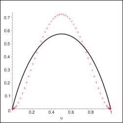
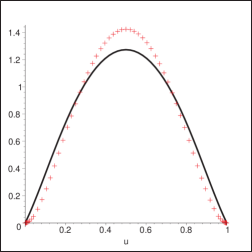
Figure 8: The two–particle twist–four DA $\mathbb{A}_{T}(u)$ without (left) and with (right) the Wandzura–Wilczek terms. Each figure compares between the renormalon model (full line) and model of Ref. [12] (crosses) which uses the first two orders in the conformal expansion with the sum–rule estimate of Eq. (5.42). Note the different scales on the vertical axis.

6 Conclusions

In this paper we have presented for the first time a systematic analysis of twist–four meson distribution amplitudes that goes beyond the first few orders in the conformal expansion. Our analysis is based on the study of the high–order behavior of perturbation theory in the single–dressed–gluon approximation which is equivalent to the study of one–loop power divergences of the contributing twist–four operators. In general, this calculation supports the conjecture that the shape of higher–twist DA is not far from the asymptotic form which is associated with operators with the lowest conformal spin. However, we find that the conformal expansion of the renormalon model does not converge uniformly at the end points. Consequently, the end–point behavior corresponding to the situation where one valence quark is soft, is qualitatively different between the sum over all spins and any fixed order in the conformal expansion. As the principal result, we obtain that the two–particle twist–four DA that describes the $k_{\perp}^{2}$ distribution of valence quarks in the meson — $\phi^{(4)}_{1}(u)$ for pion, $\mathbb{A}(u)$ and $\mathbb{A}^{T}(u)$ for $\rho$–meson — has the same linear falloff $\sim u(1-u)$ at $u\to 0,1$ as the leading–twist DA, compared to the quadratic behavior $\sim u^{2}(1-u)^{2}$ of the asymptotic DA (lowest conformal spin). Taking into account the limitations of our analysis this has to be understood as an upper bound. The existence of such a bound is important for proofs of factorization theorems.

An attractive feature of the renormalon approach is that it allows one to construct simple models of higher–twist DA with minimum number of non-perturbative parameters. In this paper we constructed such models for the pion and for the $\rho$-meson with both the longitudinal and the transverse polarizations. The corresponding expressions are given in Sect. 3, 5.1.2 and 5.2.2, respectively. In each of these cases the entire set of twist–four DA is determined in terms of the leading–twist DA with just one free parameter, the overall normalization, corresponding to the matrix element of a certain local operator. This approach presents a viable alternative to the models of Refs. [6, 12] based on the two first orders in the conformal expansion. The spread between the predictions of these two approaches is a fair measure of uncertainty in our present understanding of higher–twist effects.

In addition to giving, for the first time, an upper bound for the possible contribution of the operators with large conformal spins $J$, the renormalon model can also be used to estimate the next–to–lowest spin $J=4$ contributions. The corresponding estimates are given in Eq. (4.12), Eq. (5.20) and Eq. (5.43) for the pion, longitudinal $\rho$–meson and transverse $\rho$–meson, respectively. These estimates are probably more reliable than the corresponding QCD sum–rule results, as it is known that the sum–rule approach does not work well for operators containing derivatives. In particular for the longitudinal $\rho$–meson there is a significant difference, compare Eq. (5.20) and Eq. (5.18).

The renormalon approach can be applied in a straightforward manner to study yet higher power corrections, of twist six and above, which are otherwise inaccessible. Higher infrared–renormalon ambiguities in the coefficient functions of Eq. (2.21) at $w_{0}=2,3$, etc. corresponding to twist six, eight, etc. can be extracted from Eq. (2.22) and Eq. (2.23) in full analogy with the calculation of the leading renormalon ambiguity in Sect. 2.2.2. Assuming for simplicity the asymptotic leading–twist DA, the ambiguities in the leading–twist part of $G_{1}$ read:

$$\delta_{\hbox{\tiny IR}}^{w=2}\left\{C_{1}\otimes\phi_{\pi}\right\} = -\frac{\pi C_{F}}{2\beta_{0}}\frac{{\rm e}^{\frac{10}{3}}}{4^{2}}\left(-\Delta^{2}\Lambda^{2}\right)^{2}\,2\left[u^{3}\ln(u)+\bar{u}^{3}\ln(\bar{u})+u\bar{u}\right],$$ (6.1)

$$\delta_{\hbox{\tiny IR}}^{w=3}\left\{C_{1}\otimes\phi_{\pi}\right\} = -\frac{\pi C_{F}}{2\beta_{0}}\frac{{\rm e}^{\frac{15}{3}}}{4^{3}}\left(-\Delta^{2}\Lambda^{2}\right)^{3}\,\frac{8}{3}u\bar{u}\left[1+7u\bar{u}\right],$$

$$\delta_{\hbox{\tiny IR}}^{w=4}\left\{C_{1}\otimes\phi_{\pi}\right\} = -\frac{\pi C_{F}}{2\beta_{0}}\frac{{\rm e}^{\frac{20}{3}}}{4^{4}}\left(-\Delta^{2}\Lambda^{2}\right)^{4}\,\frac{1}{75}u\bar{u}\left[31+199u\bar{u}-2u^{2}\bar{u}^{2}\right].$$

In general, we find in the renormalon approach that the asymptotic behavior of the form $\sim u\bar{u}$ persists in the case of $G_{1}$ to all twists. For $G_{2}$, on the other hand, we find at any twist higher than four an asymptotic behavior of the form $\sim u^{2}\bar{u}^{2}$. This result suggests that the DA of all twists probably have the same universal power behavior in the end–point regions. This strong conjecture implies, in particular, that the twist expansion breaks down owing to the increasing singularity of higher–twist coefficient functions.

The present study can be extended in several respects. From the theoretical point of view the renormalon calculation that uses the modified gluon propagator in Eq. (2.20) can be understood as changing the scaling dimension of the gluon field. It is, therefore, tempting to try to reconcile the renormalon model with conformal symmetry of QCD with modified conformal spin assignment for the fields. Alternatively, since the renormalon model predictions effectively reduce to the analysis of quadratic divergences of twist–four operators, they may have the symmetry of QCD in two dimensions. Finally, there is a general problem of going beyond the large–$\beta_{0}$ approximation and taking anomalous dimensions into account.

To summarize, we believe that the renormalon approach is useful for understanding the structure of higher–twist contributions in hard exclusive processes and allows one to obtain quantitative estimates. Phenomenological applications are numerous but go beyond the tasks of this work.

Appendices

Appendix A Single–dressed–gluon calculation of the twist–two coefficient function

In this Appendix we present the detailed calculation of the diagrams in Fig. 1 to arrive at the Borel–regularized expression for the leading–twist coefficient function of the non–local operator in Eq. (2.1). The calculation is done in the Feynman gauge and for brevity we do not write explicitly the Wilson line connecting operators at different points.

We begin with Diagram 1 in Fig. 1 where the gluon is exchanged between the quark and the Wilson line. The latter is defined by Eq. (2.2). The calculation of this diagram plus its symmetric counterpart, where the gluon line is attached to the other quark, yields:

$$\left\langle p_{2}\left|{\rm T}\{\bar{d}(x_{2})\gamma_{\nu}\gamma_{5}u(x_{1})\}\right|p_{1}\right\rangle_{1} = \frac{4\pi^{2}C_{F}}{\beta_{0}}\int_{0}^{\infty}\!dw\,{\rm e}^{\frac{5}{3}w}\,(-\Lambda^{2})^{w}\int_{0}^{1}\!da\,e^{i(p_{2}x_{2}-p_{1}x_{1})}$$ (A.1)

$$\times\,\left[\bar{d}_{p_{2}}\gamma_{\sigma}\gamma_{\mu}\gamma_{\nu}\gamma_{5}u_{p_{1}}\Delta^{\sigma}{\rm I}_{1}^{\mu}(p_{2},a\Delta)+\bar{d}_{p_{2}}\gamma_{\nu}\gamma_{5}\gamma_{\mu}\gamma_{\sigma}u_{p_{1}}\Delta^{\sigma}{\rm I}_{1}^{\mu}(p_{1},a\Delta)\right],$$

where $\bar{d}_{p_{2}}$ and $u_{p_{1}}$ are quark spinors, $\Delta=x_{2}-x_{1}$ and the momentum integral ${\rm I}_{1}^{\mu}(p,\Delta)$ is given by

$${\rm I}_{1}^{\mu}(p,z) = \int\!\frac{d^{4}k}{(2\pi)^{4}}{\rm e}^{-ik\Delta}\frac{(p+k)^{\mu}}{(k^{2})^{1+w}(p+k)^{2}}$$ (A.2)

$$= \frac{1}{16\pi^{2}}\frac{\Gamma(-w)}{\Gamma(1+w)}\left(\frac{z^{2}}{4}\right)^{w}\int_{0}^{1}\!db\,b^{w}{\rm e}^{i(1-b)p\Delta}\left(ibp-2w\frac{\Delta}{\Delta^{2}}\right)^{\mu}\,.$$

Inserting the result of the momentum integration into Eq. (A.1), contracting the indices and using the Dirac equation for massless quarks gives

$$\left<p_{2}\left|{\rm T}\{\bar{d}(x_{2})\gamma_{\nu}\gamma_{5}u(x_{1})\}\right|p_{1}\right>_{1} = -\frac{C_{F}}{2\beta_{0}}\int_{0}^{\infty}\!\!dw\,{\rm e}^{\frac{5}{3}w}\,\frac{\Gamma(-w)}{\Gamma(1+w)}\left(\frac{-\Lambda^{2}\Delta^{2}}{4}\right)^{w}\!\int_{0}^{1}\!\!da\,a^{2w}\int_{0}^{1}\!\!db\,b^{w}$$

$$\times\,\left[\left(-ibp_{2}\cdot\Delta+\frac{w}{a}\right){\rm e}^{ia(1-b)p_{2}\cdot\Delta}+\left(-ibp_{1}\cdot\Delta+\frac{w}{a}\right){\rm e}^{ia(1-b)p_{1}\cdot\Delta}\right]$$

$$\times\,e^{i(p_{2}x_{2}-p_{1}x_{1})}\bar{d}_{p_{2}}\gamma_{\nu}\gamma_{5}u_{p_{1}}.$$

The terms proportional to $p_{1(2)}\cdot\Delta$ can be removed using $-ip\cdot\Delta{\rm e}^{ia(1-b)p\cdot\Delta}=\frac{1}{a}\frac{d}{db}{\rm e}^{ia(1-b)p\cdot\Delta}$ and then integrating by parts. Now the dependence on the external momenta is only in the spinors and the phase and can be absorbed in external quark states, so that the result takes the form:

$$\left<p_{2}\left|{\rm T}\{\bar{d}(x_{2})\gamma_{\nu}\gamma_{5}u(x_{1})\}\right|p_{1}\right>_{1} = -\frac{C_{F}}{2\beta_{0}}\int_{0}^{\infty}\!dw\,{\rm e}^{\frac{5}{3}w}\,\frac{\Gamma(-w)}{\Gamma(1+w)}\left(\frac{-\Lambda^{2}\Delta^{2}}{4}\right)^{w}\int_{0}^{1}\!d\alpha\int_{0}^{1-\alpha}\!\!d\beta$$ (A.4)

$$\times\int_{0}^{1}\!\!da\,a^{2w-1}\Big{\{}-2\delta(\alpha)\delta(\beta)+\int_{0}^{1}\!\!db\,b^{w}\left[\delta(\beta)\delta\left(\alpha-a(1-b)\right)+\delta(\alpha)\delta\left(\beta-a(1-b)\right)\right]\Big{\}}$$

$$\times\left<p_{2}\left|\bar{d}(x_{2}+\alpha\Delta)\gamma_{\nu}\gamma_{5}u(x_{1}-\beta\Delta)\right|p_{1}\right>.$$

Here we introduced for later convenience two new variables $\alpha$ and $\beta$. The integration over $a$ can be taken and after rearranging the terms the result can be represented as an OPE

$${\rm T}\{\bar{d}(x_{2})\gamma_{\nu}\gamma_{5}u(x_{1})\}_{1} = \frac{C_{F}}{2\beta_{0}}\,\int_{0}^{\infty}\!dw\,{\rm e}^{\frac{5}{3}w}\,\frac{\Gamma(-w)}{\Gamma(1+w)}\left(\frac{-\Delta^{2}\Lambda^{2}}{4}\right)^{w}\,\int_{0}^{1}d\alpha\int_{0}^{1-\alpha}d\beta$$ (A.5)

$$\times\,\bigg{[}(1+w)\bigg{(}f_{+}^{(w)}(\beta)\delta(\alpha)+f_{+}^{(w)}(\alpha)\delta(\beta)\bigg{)}-w\bigg{(}f^{(w)}(\beta)\delta(\alpha)+f^{(w)}(\alpha)\delta(\beta)\bigg{)}\bigg{]}$$

$$\times\,\bar{d}(x_{2}+\alpha\Delta)\gamma^{\mu}\gamma_{5}u(x_{1}-\beta\Delta)\,,$$

where it is understood that only leading–twist operators are retained on the right–hand side,

$$f^{(w)}(\beta) \equiv \beta^{2w-1}\int_{0}^{1-\beta}db\,(1-b)^{-2w}b^{w}$$ (A.6)

$$= \frac{\beta^{2w-1}(1-\beta)^{1+w}}{1+w}\,_{2}\!F_{1}([2w,w+1],[2+w];1-\beta),$$

and the “$+$” prescription is defined, as usual, by Eq. (2.26).

Next we consider Diagram 2 where the gluon is exchanged between the quarks. This contribution reads:

$$\left<p_{2}\left|{\rm T}\{\bar{d}(x_{2})\gamma_{\nu}\gamma_{5}u(x_{1})\}\right|p_{1}\right>_{2} = -\frac{i8\pi^{2}C_{F}}{\beta_{0}}\int_{0}^{\infty}\!dw\,{\rm e}^{\frac{5}{3}w}\,(-\Lambda^{2})^{w}\,e^{i(p_{2}x_{2}-p_{1}x_{1})}$$ (A.7)

$$\,\times\,\bar{d}_{p_{2}}\gamma_{\mu}\gamma_{\nu}\gamma_{5}\gamma_{\sigma}u_{p_{1}}{\rm I}_{2}^{\mu\sigma}(p_{1},p_{2},\Delta)\,,$$

where the integral ${\rm I}_{2}^{\mu\sigma}(p_{1},p_{2},\Delta)$ is given by the expression:

$${\rm I}_{2}^{\mu\sigma}(p_{1},p_{2},\Delta) = \int\!\frac{d^{4}k}{(2\pi)^{4}}{\rm e}^{-ik\Delta}\frac{(p_{1}+k)^{\mu}(p_{2}+k)^{\sigma}}{(k^{2})^{1+w}(p_{1}+k)^{2}(p_{2}+k)^{2}}$$

$$= \frac{i}{32\pi^{2}}\frac{\Gamma(-w)}{\Gamma(1+w)}\left(\frac{\Delta^{2}}{4}\right)^{w}\int_{0}^{1}\!d\alpha\int_{0}^{1-\alpha}\!d\beta\,(1-\alpha-\beta)^{w}$$

$$\,\times\,{\rm e}^{i(\alpha p_{2}\Delta+\beta p_{1}\Delta)}\left\{\left[g^{\mu\sigma}+2w\frac{\Delta^{\mu}\Delta^{\sigma}}{\Delta^{2}}\right]+\ldots\right\}.$$

Here the dots represent terms proportional to at least one external momentum $p_{1(2)}^{\mu(\sigma)}$, which do not contribute to Eq. (A.7) by virtue of the Dirac equation. Inserting Eq. (A) in Eq. (A.7), contracting the indices and absorbing the dependence on the momenta $p_{1}$ and $p_{2}$ in external quark states, one immediately obtains

$${\rm T}\{\bar{d}(x_{2})\gamma_{\nu}\gamma_{5}u(x_{1})\}_{2} = \frac{C_{F}}{2\beta_{0}}\int_{0}^{\infty}\!dw\,{\rm e}^{\frac{5}{3}w}\,\frac{\Gamma(-w)}{\Gamma(1+w)}\left(\frac{-\Lambda^{2}\Delta^{2}}{4}\right)^{w}\int_{0}^{1}\!d\alpha\int_{0}^{1-\alpha}\!d\beta\,$$ (A.9)

$$\times\,(1-\alpha-\beta)^{w}\left[g_{\mu\nu}(1+w)-2w\frac{\Delta_{\mu}\Delta_{\nu}}{\Delta^{2}}\right]$$

$$\times\,\bar{d}(x_{2}+\alpha\Delta)\gamma^{\mu}\gamma_{5}u(x_{1}-\beta\Delta)\,.$$

For the last step it was important to consider a non-forward matrix element ($p_{1}\neq p_{2}$), because otherwise one could not identify how the quark–field operators get shifted.

The last contribution comes from Diagram 3 since Diagram 4, describing the self energy of the incoming quark, has no scale and thus vanishes. We obtain:

$${\rm T}\{\bar{d}(x_{2})\gamma_{\nu}\gamma_{5}u(x_{1})\}_{3}=\frac{i4\pi^{2}C_{F}}{\beta_{0}}\Delta^{2}\!\!\int_{0}^{\infty}\!\!\!\!dw\,{\rm e}^{\frac{5}{3}w}\,(-\Lambda^{2})^{w}{\rm I}_{3}(\Delta)\bar{d}(x_{2})\gamma_{\nu}\gamma_{5}u(x_{1})\,,$$ (A.10)

where

$${\rm I}_{3}(\Delta^{2})=\int_{0}^{1}\!da\int_{0}^{a}\!db\,\int\!\frac{d^{4}k}{(2\pi)^{4}}{\rm e}^{-i(a-b)k\Delta}\frac{1}{(k^{2})^{1+w}}=\frac{i}{32\pi^{2}}\frac{\Gamma(-w)}{(1-2w)\Gamma(1+w)}\left(\frac{\Delta^{2}}{4}\right)^{w-1}.$$ (A.11)

Collecting the contributions in Eq. (A.5), Eq. (A.9) and Eq. (A.10) we get a gauge–invariant result for the OPE of the T–product of quark fields to all orders in the strong coupling in in the large-$\beta_{0}$ limit:

$${\rm T}\{\bar{d}(x_{2})\gamma_{\nu}\gamma_{5}[x_{2},x_{1}]u(x_{1})\} = \frac{C_{F}}{2\beta_{0}}\,\int_{0}^{\infty}\!dw\,{\rm e}^{\frac{5}{3}w}\,\frac{\Gamma(-w)}{\Gamma(1+w)}\left(\frac{-\Delta^{2}\Lambda^{2}}{4}\right)^{w}\,\int_{0}^{1}d\alpha\int_{0}^{1-\alpha}d\beta$$

$$\times\bigg{\{}g_{\mu\nu}\,\bigg{[}(1+w)\bigg{(}f_{+}^{(w)}(\beta)\delta(\alpha)+f_{+}^{(w)}(\alpha)\delta(\beta)\bigg{)}-w\bigg{(}f^{(w)}(\beta)\delta(\alpha)+f^{(w)}(\alpha)\delta(\beta)\bigg{)}\bigg{]}$$

$$+\,\left(g_{\mu\nu}(1+w)\,-w\frac{2\Delta_{\mu}\Delta_{\nu}}{\Delta^{2}}\right)\,(1-\alpha-\beta)^{w}$$

$$-\,g_{\mu\nu}\frac{1}{1-2w}\delta(\alpha)\delta(\beta)\bigg{\}}\,\times\,\bar{d}(x_{2}+\alpha\Delta)\gamma^{\mu}\gamma_{5}[x_{2}+\alpha\Delta,x_{1}-\beta\Delta]u(x_{1}-\beta\Delta),$$

where the terms in the curly brackets are grouped as they appear from individual diagrams in Feynman gauge: the first line corresponds to Diagram 1 (vertex correction) in Fig. 1 and its symmetric counterpart, the second line to Diagram 2 (box diagram), and the third line to Diagram 3 (self–energy like correction to the Wilson line). Disentangling the two Lorentz structures we end up with the answers for the unrenormalized coefficient functions given in Eq. (2.22) and Eq. (2.23).

Appendix B The operator $\bar{d}\gamma_{\mu}\gamma_{5}gD_{\alpha}G^{\alpha\beta}u$: UV divergence and EOM relations

The calculation of the UV–renormalon ambiguity of the operator in Eq. (2.1) goes along the same lines as in Sect. 2.3 and is fully analogous to the similar calculation (with no $\gamma_{5}$) in [17, 31]. For the matrix element between off–shell quark states (Fig. 2) we get

$$\left<q_{2}\left|\bar{d}(-z)gD^{\alpha}G_{\alpha\beta}(vz)\Gamma u(z)\right|q_{1}\right>\, = \,i\frac{4\pi^{2}C_{F}}{\beta_{0}}{\rm e}^{-i(q_{1}+q_{2})z}\,\left(g^{\sigma\rho}g_{\beta\nu}-g^{\rho}_{\beta}g^{\sigma}_{\nu}\right)$$

$$\times\int_{0}^{\infty}\!\!\!dw\,{\rm e}^{\frac{5}{3}w}(-\Lambda^{2})^{w}\,\Big{[}\bar{d}_{q_{2}}\gamma^{\nu}\gamma^{\lambda}\Gamma u_{q_{1}}\,\bar{I}_{\lambda\sigma\rho}(q_{2},(1+v)z)+\bar{d}_{q_{2}}\Gamma\gamma^{\lambda}\gamma^{\nu}u_{q_{1}}\,\bar{I}_{\lambda\sigma\rho}(q_{1},(1-v)z)\Big{]},$$

where the momentum integral is

$$\bar{I}_{\lambda\sigma\rho}(q,z)=\int\frac{d^{4}k}{(2\pi)^{4}}\frac{(q+k)_{\lambda}k_{\sigma}k_{\rho}}{\left(k^{2}\right)^{(1+w)}(q+k)^{2}}\,{\rm e}^{-ikz}.$$ (B.2)

Computing the integral, extracting the $w=1$ residue, specifying $\Gamma=\gamma_{\mu}\gamma_{5}$ and projecting with $x^{\mu}x^{\beta}$ we obtain the result in Eq. (2.39). Taking the matrix element of Eq. (2.39) between the vacuum and a pion state we end up with the renormalon ambiguity of the DA $\Xi_{\pi}(\alpha_{i})$ given in the last line of Eq. (2.3).

Going from an ambiguity to a model involves a replacement of the large–$\beta_{0}$ renormalon residue by a physical non-perturbative parameter, a certain local matrix element. From [6] it is known that the normalization of all four DA $\Phi_{\perp,\parallel}$ and $\Psi_{\perp,\parallel}$ is controlled by a single non-perturbative parameter $\delta^{2}$ for $J=3$. In the renormalon model, contributions of higher spins $J=4,5,\ldots$ to $\Phi_{\perp,\parallel}$ and $\Psi_{\perp,\parallel}$ are fixed uniquely in terms of $\delta^{2}$ so that no new parameters appear. We are going to argue that within this construction the normalization of $\Xi_{\pi}$ is also fixed uniquely by EOM that relate it to the $J=5$ contributions to the other DA. Thus, all five DA are given in terms of $\delta^{2}$ and the leading–twist pion DA.

The necessary constraint can be derived from the operator identity for the second derivative

$$\frac{\partial^{2}}{\partial x_{\alpha}\partial x^{\alpha}}\bar{d}(-x)\Gamma\,u(x)=-\partial^{2}\bar{d}(-x)\Gamma\,u(x)+g\bar{d}(-x)\Big{[}\sigma G(-x)\,\Gamma+\Gamma\sigma G(x)\Big{]}u(x)$$ (B.3)

$$+ {}2igx^{\nu}\frac{\partial}{\partial x_{\mu}}\!\int_{-1}^{1}\!\!dv\,v\,\bar{d}(-x)\Gamma G_{\nu\mu}(vx)u(x)+2igx^{\nu}\partial_{\mu}\!\int_{-1}^{1}\!\!dv\,\bar{d}(-x)\Gamma G_{\nu\mu}(vx)u(x)$$

$${}+2g\int_{-1}^{1}\!dv\int_{-1}^{v}\!dt\,(1+vt)\bar{d}(-x)\Gamma x^{\mu}x^{\nu}G_{\mu\rho}(-vx)G^{\rho}_{\phantom{\nu}\nu}(-tx)u(x)$$

$${}-igx^{\nu}\int_{-1}^{1}\!\!dv\,(1+v^{2})\,\bar{d}(-x)\Gamma[D_{\mu},G^{\mu}_{\phantom{\nu}\nu}](vx)u(x)$$

given in Eq. (A.9) in [12] (see also [26]). Here $\sigma G\equiv\sigma_{\alpha\beta}G^{\alpha\beta}$ and $\partial_{\mu}$ stands for the derivative with respect to the total translation.

Taking the matrix element of (B.3) between the vacuum and a pion state and using the definitions of the DA we obtain

$$2\,i\,\int_{0}^{1}du{\rm e}^{-i\,\mathit{pz}\,(2\,u-1)}\,\bigg{[}(4-2\,i\,\mathit{pz}\,(2\,u-1))\,\phi_{1}(u)+(-3+i\mathit{pz}\,(2\,u-1))\,\phi_{2}(u)\bigg{]}$$

$$=\int D\alpha_{i}\,\,{\rm e}^{-i\,\mathit{pz}\,(\alpha_{1}-\alpha_{2})}\bigg{[}2\left(\left({\frac{1}{\mathit{pz}^{2}\,\alpha_{3}^{2}}}-1\right)\,\mathrm{sin}(\mathit{pz}\,\alpha_{3})-{\frac{\mathrm{cos}(\mathit{pz}\,\alpha_{3})}{\mathit{pz}\,\alpha_{3}}}\right)\,{\Phi_{\perp}(\alpha_{i})}$$

$$\!\!+\left(\left({\frac{1}{\alpha_{3}}}+2-{\frac{i\,\alpha_{1}}{\mathit{pz}\,\alpha_{3}^{2}}}+{\frac{i\,\alpha_{2}}{\mathit{pz}\,\alpha_{3}^{2}}}\right)\,\mathrm{sin}(\mathit{pz}\,\alpha_{3})+\frac{i}{\alpha_{3}}\,({\alpha_{1}}-{\alpha_{2}})\,\mathrm{cos}(\mathit{pz}\,\alpha_{3})\right)\,{\Phi_{\parallel}(\alpha_{i})}$$ (B.4)

$$\!\!+\left(\left({\frac{1}{\alpha_{3}}}-{\frac{1}{\mathit{pz}^{2}\,\alpha_{3}^{3}}}\right)\,\mathrm{sin}(\mathit{pz}\,\alpha_{3})+{\frac{\mathrm{cos}(\mathit{pz}\,\alpha_{3})}{\mathit{pz}\,\alpha_{3}^{2}}}\right)\Xi_{\pi}(\alpha_{i})+i\left(2{\Psi_{\perp}(\alpha_{i})}-{\Psi_{\parallel}(\alpha_{i})}\right)\,\mathrm{cos}(\mathit{pz}\,\alpha_{3})\bigg{]},$$

where we omitted the contributions of the two–gluon operator from the right–hand side. These can be systematically put to zero to our accuracy as they start contributing at higher order in the flavor expansion.

Expansion of Eq. (B) in powers of $pz$ yields simple relations between integrals that involve all five three–particle DA. The odd powers are trivial: both the right–hand side and the left–hand side vanish by symmetry. The first two non-trivial relations are:

$$\int_{0}^{1}du\Big{[}-8\,\phi_{1}(u)+6\,\phi_{2}(u)\Big{]}=\int D\alpha_{i}\,\,\Big{[}-2\,{{\Psi_{\perp}(\alpha_{i})}}+\,{{\Psi_{\parallel}(\alpha_{i})}}\Big{]},$$ (B.5)

$$\int_{0}^{1}du\,(u-\bar{u})^{2}\,\Big{[}-16\,\phi_{1}(u)+10\,\phi_{2}(u)\Big{]}=\int D\alpha_{i}\,\,\bigg{[}-{\frac{4}{3}}\,(\alpha_{1}-\alpha_{2})\,\Xi_{\pi}(\alpha_{i})$$

$$\hskip 30.0pt+{\frac{2}{3}}\,(\alpha_{1}-\alpha_{2})\left(7\,(\alpha_{1}+\alpha 2\right)-10)\,{\Phi_{\parallel}(\alpha_{i})}-{\frac{8}{3}}\,(\alpha_{1}-\alpha_{2})(\alpha_{1}+\alpha_{2}-1)\,\Phi_{\perp}(\alpha_{i})$$

$$\hskip 30.0pt\mbox{}+\left(1-2\,\alpha_{2}-2\,\alpha_{1}+2\,\alpha_{2}^{2}+2\,\alpha_{1}^{2}\right)\,{{\left(\Psi_{\parallel}(\alpha_{i})-2\Psi_{\perp}(\alpha_{i})\right)}}\bigg{]}.$$

The first relation does not involve $\Xi_{\pi}(\alpha_{i})$ and is satisfied identically both by the model of [6] and the renormalon model. The second relation gives the required constraint for the normalization integral $\int{\cal D}\alpha_{i}\,(\alpha_{1}-\alpha_{2})\,\Xi_{\pi}(\alpha_{i})$ in terms of the other four DA. It is easy to verify that in order to satisfy this constraint one must assume in the last line of Eq. (2.3) the same replacement $c\Lambda^{2}\longrightarrow\delta^{2}/6$ as in the other DA.

Appendix C Cancellation of renormalons for the $\rho$–meson amplitudes

Here we want to demonstrate cancellation of IR renormalon ambiguities in the leading–twist coefficient functions with the UV–renormalon ambiguities in the matrix elements of twist–four DA for the case of exclusive amplitudes involving a vector $\rho$–meson. Similarly to the pion case, we consider the simplest example: a gauge–invariant T–product of quark fields sandwiched between the vacuum and the meson state.

C.1 UV renormalons in two–particle DA

To begin with, we calculate the UV–renormalon ambiguities in the two–particle DA of twist four. These can be obtained from the three–particle ones using EOM.

The specific EOM relations we need in the chiral–even sector are [12]:

$$g_{3}(u) = \phi_{\parallel}-2\frac{d}{du}\int_{0}^{u}\!d\alpha_{1}\int_{0}^{1-u}\!d\alpha_{2}\frac{1}{\alpha_{3}}\left[2\Phi(\alpha_{i})+\Psi(\alpha_{i})\right]$$

$$\mathbb{A}(u) = 32\int_{0}^{u}\!dv\int_{0}^{v}\!dw\left(g^{v}_{\perp}(w)-\phi_{\parallel}(w)\right)+32\int_{0}^{u}\!dv\int_{0}^{v}\!d\alpha_{1}\int_{0}^{1-v}\!d\alpha_{2}\frac{1}{\alpha_{3}}\left[2\Phi(\alpha_{i})+\Psi(\alpha_{i})\right],$$ (C.1)

$$+8\int_{0}^{u}\!d\alpha_{1}\int_{0}^{1-u}\!d\alpha_{2}\frac{u\alpha_{2}-(1-u)\alpha_{1}}{\alpha_{3}^{2}}\left[2\Phi(\alpha_{i})+\Psi(\alpha_{i})\right].$$

This implies that the ambiguities of $g_{3}(u)$ and $\mathbb{A}(u)$ due to UV renormalons at $w=1$ are given by

$$\delta_{\hbox{\tiny UV}}\left\{g_{3}(u)\right\} = -2\frac{d}{du}\int_{0}^{u}\!d\alpha_{1}\int_{0}^{1-u}\!d\alpha_{2}\frac{1}{\alpha_{3}}\delta_{\hbox{\tiny UV}}\left\{2\Phi(\alpha_{i})+\Psi(\alpha_{i})\right\},$$

$$\delta_{\hbox{\tiny UV}}\left\{\mathbb{A}(u)\right\} = 32\int_{0}^{u}\!dv\int_{0}^{v}\!d\alpha_{1}\int_{0}^{1-v}\!d\alpha_{2}\frac{1}{\alpha_{3}}\delta_{\hbox{\tiny UV}}\left\{2\Phi(\alpha_{i})+\Psi(\alpha_{i})\right\},$$ (C.2)

$$+8\int_{0}^{u}\!d\alpha_{1}\int_{0}^{1-u}\!d\alpha_{2}\frac{u\alpha_{2}-(1-u)\alpha_{1}}{\alpha_{3}^{2}}\delta_{\hbox{\tiny UV}}\left\{2\Phi(\alpha_{i})+\Psi(\alpha_{i})\right\},$$

where the ambiguities of the three–particle DA can be read from Eq. (5.1.2) using the inverse substitution in Eq. (5.12). For $g_{3}(u)$ we get

$$\delta_{\hbox{\tiny UV}}\left\{g_{3}(u)\right\} = 4c\frac{\Lambda^{2}}{m_{\rho}^{2}}\frac{d}{du}\int_{0}^{u}\!d\alpha_{1}\int_{0}^{1-u}\!d\alpha_{2}\,\left[\frac{\phi_{\parallel}(\alpha_{1})}{(1-\alpha_{1})^{2}}-\frac{\phi_{\parallel}(\alpha_{2})}{(1-\alpha_{2})^{2}}\right]$$

$$= 4c\frac{\Lambda^{2}}{m_{\rho}^{2}}\frac{d}{du}\left[(1-u)\int_{0}^{u}d\alpha\,\frac{\phi_{\parallel}(\alpha)}{(1-\alpha)^{2}}-u\int_{0}^{1-u}d\alpha\,\frac{\phi_{\parallel}(\alpha)}{(1-\alpha)^{2}}\right],$$

where we evaluated one of the $\alpha$ integrals. Taking the derivative in respect to $u$ and using the symmetry $\phi_{\parallel}(u)=\phi_{\parallel}(1-u)$ yields the desired result:

$$\delta_{\hbox{\tiny UV}}\left\{g_{3}(u)\right\} = -4c\frac{\Lambda^{2}}{m_{\rho}^{2}}\left\{\int_{0}^{1}\!dv\,\phi_{\parallel}(v)\left[\theta(u>v)\;\frac{1}{\bar{v}^{2}}+\theta(u<v)\;\frac{1}{v^{2}}\right]-\frac{\phi_{\parallel}(u)}{u\bar{u}}\right\}.$$ (C.4)

In turn, for the DA $\mathbb{A}(u)$ we get the following expression:

$$\delta_{\hbox{\tiny UV}}\left\{\mathbb{A}(u)\right\} = -16c\frac{\Lambda^{2}}{m_{\rho}^{2}}\Bigg{\{}4\int_{0}^{u}\!dv\int_{0}^{v}\!d\alpha_{1}\int_{0}^{1-v}\!d\alpha_{2}\,\left[\frac{\phi_{\parallel}(\alpha_{1})}{(1-\alpha_{1})^{2}}-\frac{\phi_{\parallel}(\alpha_{2})}{(1-\alpha_{2})^{2}}\right]$$

$$+\int_{0}^{u}\!d\alpha_{1}\int_{0}^{1-u}\!d\alpha_{2}\,\frac{u\alpha_{2}-(1-u)\alpha_{1}}{1-\alpha_{1}-\alpha_{2}}\left[\frac{\phi_{\parallel}(\alpha_{1})}{(1-\alpha_{1})^{2}}-\frac{\phi_{\parallel}(\alpha_{2})}{(1-\alpha_{2})^{2}}\right]\Bigg{\}}.$$

Taking one of the $\alpha$ integrals in each line yields:

$$\delta_{\hbox{\tiny UV}}\left\{\mathbb{A}(u)\right\} = -16c\frac{\Lambda^{2}}{m_{\rho}^{2}}\Bigg{\{}4\int_{0}^{u}\!dv\,\left[(1-v)\int_{0}^{v}\!d\alpha\,\frac{\phi_{\parallel}(\alpha)}{(1-\alpha)^{2}}-v\int_{0}^{1-v}\!d\alpha\,\frac{\phi_{\parallel}(\alpha)}{(1-\alpha)^{2}}\right]$$

$$-\left[\int_{0}^{u}\!d\alpha\,\left((u-\alpha)\ln\left(\frac{u-\alpha}{1-\alpha}\right)+u(1-u)\right)\frac{\phi_{\parallel}(\alpha)}{(1-\alpha)^{2}}\right.$$

$$-\left.\int_{0}^{1-u}\!d\alpha\,\left((1-u-\alpha)\ln\left(\frac{1-u-\alpha}{1-\alpha}\right)+u(1-u)\right)\frac{\phi_{\parallel}(\alpha)}{(1-\alpha)^{2}}\right]\Bigg{\}}.$$

Finally, integrating by parts over $v$ in the first line and rearranging the terms we obtain:

$$\delta_{\hbox{\tiny UV}}\left\{\mathbb{A}(u)\right\} = 16c\frac{\Lambda^{2}}{m_{\rho}^{2}}\int_{0}^{1}dv\,\phi_{\parallel}(v)\Bigg{\{}\theta(u>v)\;\frac{1}{\bar{v}^{2}}\left[{\bar{u}+\bar{u}^{2}+(u-v)\ln\frac{u-v}{\bar{v}}}\right]$$ (C.7)

$$\hskip 20.0pt+\theta(u<v)\;\frac{1}{v^{2}}\left[{u+u^{2}+(v-u)\ln\frac{v-u}{v}}\right]\Bigg{\}}.$$

In the chiral–odd sector the EOM relations between the two–particle and the three–particle DA of twist four are given by [12]:

$$h_{3}(u) = 2h_{\parallel}^{(s)}(u)-\Phi_{\perp}(u)$$

$$-2\frac{d}{du}\int_{0}^{u}\!d\alpha_{1}\int_{0}^{1-u}d\alpha_{2}\left[\frac{\alpha_{1}-\alpha_{2}-(2u-1)}{\alpha_{3}^{2}}S(\alpha_{i})-\frac{1}{\alpha_{3}}\left(T_{2}(\alpha_{i})-T_{3}(\alpha_{i})\right)\right],$$

$$\mathbb{A}_{T}(u) = -2\int_{0}^{u}\!dv\,(2v-1)\left[\Phi_{\perp}(v)+h_{3}(v)\right]+8\int_{0}^{u}\!dv\int_{0}^{1-u}\!dw\left[h_{3}(w)-\Phi_{\perp}(w)\right]$$

$$+4\int_{0}^{u}\!d\alpha_{1}\int_{0}^{1-u}\!d\alpha_{2}\left[\frac{1}{\alpha_{3}}S(\alpha_{i})-\frac{\alpha_{1}-\alpha_{2}-(2u-1)}{\alpha_{3}^{2}}\left(T_{2}(\alpha_{i})-T_{3}(\alpha_{i})\right)\right].$$

As a consequence, the ambiguity of $h_{3}(u)$ and $\mathbb{A}_{T}(u)$ due to UV renormalons is related to that of the three–particle DA $S(\alpha_{i})$, $T_{2}(\alpha_{i})$ and $T_{3}(\alpha_{i})$. Using the results for the ambiguities of the three–particle DA in Eq. (5.2.2) with the inverse substitution in Eq. (5.33) we obtain

$$\delta_{\hbox{\tiny UV}}\left\{h_{3}(u)\right\} = 4c\frac{\Lambda^{2}}{m_{\rho}^{2}}\frac{d}{du}\int_{0}^{u}\!d\alpha_{1}\int_{0}^{1-u}d\alpha_{2}\left\{\left[\frac{u-\alpha_{1}}{(1-\alpha_{1}-\alpha_{2})^{2}}-\frac{1}{1-\alpha_{1}}\right]\frac{\phi_{\perp}(\alpha_{1})}{(1-\alpha_{1})}\right.$$ (C.9)

$$-\left.\left[\frac{1-u-\alpha_{2}}{(1-\alpha_{1}-\alpha_{2})^{2}}-\frac{1}{1-\alpha_{2}}\right]\frac{\phi_{\perp}(\alpha_{2})}{(1-\alpha_{2})}\right\}.$$

The square bracket in the first line vanishes upon taking the $\alpha_{2}$ integral and that in the second line upon performing the $\alpha_{1}$ integral. Thus there is no UV renormalon ambiguity (at $w=1$):

$$\delta_{\hbox{\tiny UV}}\left\{h_{3}(u)\right\} = 0.$$ (C.10)

For $\mathbb{A}_{T}(u)$ on the other hand

$$\delta_{\hbox{\tiny UV}}\left\{\mathbb{A}_{T}(u)\right\} = 8c\frac{\Lambda^{2}}{m_{\rho}^{2}}\int_{0}^{u}\!\!d\alpha_{1}\!\int_{0}^{1-u}\!\!\!\!d\alpha_{2}\left\{\left[1-\frac{2(u-\alpha_{1})}{(1-\alpha_{1}-\alpha_{2})}+\frac{(u-\alpha_{1})(1-\alpha_{1})}{(1-\alpha_{1}-\alpha_{2})^{2}}\right]\frac{\phi_{\perp}(\alpha_{1})}{(1-\alpha_{1})^{2}}\right.$$ (C.11)

$$+\left.\left[1-\frac{2(1-u-\alpha_{2})}{(1-\alpha_{1}-\alpha_{2})}+\frac{(1-u-\alpha_{2})(1-\alpha_{2})}{(1-\alpha_{1}-\alpha_{2})^{2}}\right]\frac{\phi_{\perp}(\alpha_{2})}{(1-\alpha_{2})^{2}}\right\}.$$

Taking one $\alpha$ integral we obtain

$$\delta_{\hbox{\tiny UV}}\left\{\mathbb{A}_{T}(u)\right\} = 16c\frac{\Lambda^{2}}{m_{\rho}^{2}}\int_{0}^{1}dv\,\phi_{\parallel}(v)\Bigg{[}\theta(u>v)\;\frac{1}{(1-v)^{2}}\left({(1-u)+(u-v)\ln\frac{u-v}{1-v}}\right)$$ (C.12)

$$\hskip 100.0pt+\theta(u<v)\;\frac{1}{v^{2}}\left({u+(v-u)\ln\frac{v-u}{v}}\right)\Bigg{]}.$$

C.2 IR renormalons in coefficient functions

The IR $w=1$ renormalon ambiguity in the all–order perturbative calculation of the leading–twist coefficient functions can be obtained from a generalization of the OPE relation in Eq. (A) for the case of an arbitrary Dirac matrix $\Gamma$ between the quark fields:

$$\delta_{\hbox{\tiny IR}}\left\{{\rm T}\{\bar{d}(x_{2})\Gamma u(x_{1})\}\right\} = -c\Lambda^{2}\Delta^{2}\int_{0}^{1}\!d\alpha\int_{0}^{1-\alpha}\!d\beta\,$$

$${}\times\Big{\{}\left(f^{(1)}(\beta)\delta(\alpha)+f^{(1)}(\alpha)\delta(\beta)\right)\left[\bar{d}(x_{2}+\alpha\Delta)\Gamma u(x_{1}-\beta\Delta)\right]$$

$$+\frac{1}{4}(1-\alpha-\beta)\left(g_{\mu\nu}+2\frac{\Delta_{\mu}\Delta_{\nu}}{\Delta^{2}}\right)\,\left[\bar{d}(x_{2}+\alpha\Delta)\gamma_{\alpha}\gamma^{\mu}\Gamma\gamma^{\nu}\gamma^{\alpha}u(x_{1}-\beta\Delta)\right]\Big{\}},$$

where we replaced the $w$–integral by $\pi$ times the $w=1$ residue and suppressed the gauge–link; $c$ was defined in Eq. (2.33).

For vector mesons there are two relevant structures, chiral–even $\Gamma=\gamma_{\mu}$, and chiral–odd $\Gamma=\sigma_{\mu\nu}$. We will discuss these two sectors separately.

Chiral–even amplitudes

The matrix element of the T–product of quark operators between the $\rho^{+}$ and the vacuum state contains three Lorentz structures which we parametrize using the structure function $F_{i}$:

$$\langle 0|{\rm T}\{\bar{d}(-x)\gamma_{\mu}u(x)\}|\rho^{+}(P,\lambda)\rangle_{\mu^{2}} = f_{\rho}m_{\rho}\int_{0}^{1}\!du\,e^{-ipx(u-\bar{u})}\,$$

$$\times\Bigg{\{}\frac{e^{(\lambda)}x}{Px}P_{\mu}F_{1}(u,x^{2};\mu^{2})+\left(e_{\mu}^{(\lambda)}-P_{\mu}\frac{e^{(\lambda)}x}{Px}\right)F_{2}(u,x^{2};\mu^{2})-\frac{1}{2}x_{\mu}\frac{e^{(\lambda)}x}{(Px)^{2}}m_{\rho}^{2}F_{3}(u,x^{2};\mu^{2})\Bigg{\}}.$$

The OPE to twist–four accuracy reads:

$$F_{1}(u,x^{2};\mu^{2}) = C_{1}^{(2)}\otimes\phi_{\parallel}(u)+\frac{m_{\rho}^{2}x^{2}}{4}\mathbb{A}(u)\,,$$

$$F_{2}(u,x^{2};\mu^{2}) = C_{2}^{(3)}\otimes g_{\perp}^{(v)}(u)+\ldots\,,$$

$$F_{3}(u,x^{2};\mu^{2}) = C_{3}^{(2)}\otimes\phi_{\parallel}(u)+\mathbb{C}(u).$$ (C.15)

Here $\phi_{\parallel}(u)$ is the leading–twist DA of the longitudinally polarized $\rho$–meson, $g_{\perp}^{(v)}(u)$ is the DA of twist–three corresponding to the contribution of the transversely polarized $\rho$–meson and the functions $\mathbb{A}(u)$, $\mathbb{C}(u)$ represent higher–twist contributions. At leading order in $\alpha_{s}$ $C_{1}^{(2)}(u,v)=C_{2}^{(3)}(u,v)=\delta(u-v)$, alias $F_{1}(u,x^{2};\mu^{2})=\phi_{\parallel}(u)$ and $F_{2}(u,x^{2};\mu^{2})=g_{\perp}^{(v)}(u)$, while the remaining twist–two coefficient function $C_{3}^{(2)}$ vanishes.

In order to calculate the IR–renormalon ambiguity in the leading–twist part of the amplitudes in Eq. (C.2) we take the appropriate matrix element of Eq. (C.2) retaining the leading terms in Eq. (C.2). The result reads :

$$\delta_{\hbox{\tiny IR}}\left\{C_{1}^{(2)}\otimes\phi_{\parallel}(u)\right\} \!=\! \frac{-16c\Lambda^{2}}{m_{\rho}^{2}}\int_{0}^{1}\!dv\int_{0}^{1}\!d\alpha\int_{0}^{1-\alpha}\!d\beta\,\delta\big{(}v(1-\alpha-\beta)+\alpha-u\big{)}\,\phi_{\parallel}(v)$$

$$\hskip 90.0pt\times\left[\left(f^{(1)}(\beta)\delta(\alpha)+f^{(1)}(\alpha)\delta(\beta)\right)+2(1-\alpha-\beta)\right]$$

$$= \frac{-16c\Lambda^{2}}{m_{\rho}^{2}}\int_{0}^{1}dv\,\phi_{\parallel}(v)\bigg{[}\theta(u<v)\;\frac{1}{v^{2}}\left({u+u^{2}+(v-u)\ln\frac{v-u}{v}}\right)$$

$$\hskip 90.0pt+\theta(u>v)\;\frac{1}{\bar{v}^{2}}\left({\bar{u}+\bar{u}^{2}+(u-v)\ln\frac{u-v}{\bar{v}}}\right)\bigg{]},$$

$$\delta_{\hbox{\tiny IR}}\left\{C_{3}^{(2)}\otimes\phi_{\parallel}(u)\right\} = \frac{4c\Lambda^{2}}{m_{\rho}^{2}}\frac{d^{2}}{du^{2}}\int_{0}^{1}\!dv\!\int_{0}^{1}\!\!d\alpha\!\int_{0}^{1-\alpha}\!\!\!\!\!\!\!d\beta(1\!-\!\alpha\!-\!\beta)\,\delta\big{(}v(1\!-\!\alpha\!-\!\beta)+\alpha-u\big{)}\,\phi_{\parallel}(v)$$ (C.16)

$$= \frac{4c\Lambda^{2}}{m_{\rho}^{2}}\left\{\int_{0}^{1}\!dv\,\phi_{\parallel}(v)\left[\theta(u>v)\;\frac{1}{\bar{v}^{2}}+\theta(u<v)\;\frac{1}{v^{2}}\right]-\frac{\phi_{\parallel}(u)}{u\bar{u}}\right\}.$$

Comparing these expressions with the UV–renormalon ambiguities in the twist–four contributions for $\mathbb{A}(u)$ and $\mathbb{C}(u)$ in Eq. (C.7) and Eq. (C.4), respectively, we observe that the ambiguities in the structure functions $F_{i}$ cancel out, as expected.

Chiral–odd amplitudes

The calculation for chiral-odd amplitudes goes along similar lines. We parametrize the matrix element in terms of three more structure functions

$$\langle 0|\bar{d}(-x)\sigma_{\mu\nu}u(x)|\rho^{+}(P,\lambda)\rangle=if_{\rho}^{T}\int_{0}^{1}\!du\,e^{-ipx(u-\bar{u})}\bigg{\{}\left(e^{(\lambda)}_{\mu}P_{\nu}-e^{(\lambda)}_{\nu}P_{\mu}\right)F^{T}_{1}(u,x^{2};\mu^{2})$$ (C.17)

$$+\left(P_{\mu}x_{\nu}-P_{\nu}x_{\mu}\right)\frac{e^{(\lambda)}x}{(Px)^{2}}m_{\rho}^{2}F^{T}_{2}(u,x^{2};\mu^{2})+\frac{1}{2}\left(e^{(\lambda)}_{\mu}x_{\nu}-e^{(\lambda)}_{\nu}x_{\mu}\right)\frac{m_{\rho}^{2}}{Px}F^{T}_{3}(u,x^{2};\mu^{2})\bigg{\}}.$$

To twist–four accuracy

$$F^{T}_{1}(u,x^{2};\mu^{2}) = {C}_{1}^{T(2)}\otimes\phi_{\perp}(u)+\frac{m_{\rho}^{2}x^{2}}{4}\mathbb{A}_{T}(u)\,,$$

$$F^{T}_{2}(u,x^{2};\mu^{2}) = {C}_{2}^{T(3)}\otimes h_{\parallel}^{(t)}(u)+\ldots\,,$$

$$F^{T}_{3}(u,x^{2};\mu^{2}) = {C}_{3}^{T(2)}\otimes\phi_{\perp}(u)+\mathbb{C}_{T}(u)\,,$$ (C.18)

where $\phi_{\perp}(u)$ parametrize the leading–twist part. Repeating the procedure of the previous section we obtain the following ambiguity:

$$\delta_{\hbox{\tiny IR}}\left\{{C}_{1}^{T(2)}\otimes\phi_{\perp}(u)\right\} = -16c\frac{\Lambda^{2}}{m_{\rho}^{2}}\int_{0}^{1}dv\int_{0}^{1}d\alpha\int_{0}^{1-\alpha}\!d\beta\,\delta\left(v(1-\alpha-\beta)+\alpha-u\right)\phi_{T}(v)$$

$$\hskip 90.0pt\times\left(f^{(1)}(\beta)\delta(\alpha)+f^{(1)}(\alpha)\delta(\beta)\right)$$

$$= -16c\frac{\Lambda^{2}}{m_{\rho}^{2}}\int_{0}^{1}\!dv\,\phi_{T}(v)\Bigg{[}\theta(u<v)\;\frac{1}{v^{2}}\left({u+(v-u)\ln\frac{v-u}{v}}\right)$$

$$\hskip 90.0pt+\theta(u>v)\;\frac{1}{\bar{v}^{2}}\left({\bar{u}+(u-v)\ln\frac{u-v}{\bar{v}}}\right)\Bigg{]},$$

$$\delta_{\hbox{\tiny IR}}\left\{{C}_{3}^{T(2)}\otimes\phi_{\perp}(u)\right\} = 0,$$ (C.19)

The absence of an ambiguity in ${C}_{3}^{T(2)}\otimes\phi_{\perp}(u)$, which is to be associated with $\mathbb{C}_{T}(u)$, results from the fact that Diagram 2 in Fig. 1 vanishes owing to the identity $\gamma_{\alpha}\sigma_{\mu\nu}\gamma^{\alpha}=0$. The absence of this ambiguity is expected based on the fact that $h_{3}(u)$ has no corresponding UV–renormalon ambiguity — see Eq. (C.10) — and the relation between $\mathbb{C}_{T}(u)$ and $h_{3}(u)$ in Eq. (5.2.1). Comparing the result for $\delta_{\hbox{\tiny IR}}\{{C}_{1}^{T(2)}\otimes\phi_{\perp}(u)\}$ with the UV–renormalon ambiguity in $\mathbb{A}^{T}(u)$ in Eq. (C.12) we observe that the ambiguities in the structure function $F_{1}^{T}$ cancel out. This completes the calculation.

References

• [1] A. V. Efremov and A. V. Radyushkin, Theor. Math. Phys. 42 (1980) 97 [Teor. Mat. Fiz. 42 (1980) 147]. Phys. Lett. B94 (1980) 245.
• [2] G. P. Lepage and S. J. Brodsky, Phys. Lett. B87 (1979) 359; Phys. Rev. D22 (1980) 2157.
• [3] V. M. Braun, “Light-cone sum rules,” hep-ph/9801222; P. Colangelo and A. Khodjamirian, “QCD sum rules: A modern perspective,” hep-ph/0010175.
• [4] C. W. Bauer, D. Pirjol and I. W. Stewart, Phys. Rev. D67 (2003) 071502 [hep-ph/0211069]; M. Beneke and T. Feldmann, hep-ph/0311335.
• [5] V. M. Braun, G. P. Korchemsky and D. Muller, Prog. Part. Nucl. Phys. 51 (2003) 311 [hep-ph/0306057].
• [6] V. M. Braun and I. E. Filyanov, Z. Phys. C48 (1990) 239.
• [7] V. L. Chernyak and A. R. Zhitnitsky, Nucl. Phys. B201 (1982) 492 [Erratum-ibid. B214 (1983) 547].
• [8] V. L. Chernyak and I. R. Zhitnitsky, Nucl. Phys. B246 (1984) 52.
• [9] V. L. Chernyak, A. A. Ogloblin and I. R. Zhitnitsky, Z. Phys. C42 (1989) 569; Z. Phys. C42 (1989) 583.
• [10] V. L. Chernyak and A. R. Zhitnitsky, Phys. Rept. 112 (1984) 173.
• [11] P. Ball, V. M. Braun, Y. Koike and K. Tanaka, Nucl. Phys. B529 (1998) 323 [hep-ph/9802299].
• [12] P. Ball and V. M. Braun, Nucl. Phys. B543 (1999) 201 [hep-ph/9810475].
• [13] P. Ball, JHEP 9901 (1999) 010 [hep-ph/9812375].
• [14] V. Braun, R. J. Fries, N. Mahnke and E. Stein, Nucl. Phys. B589 (2000) 381 [Erratum-ibid. B607 (2001) 433] [hep-ph/0007279].
• [15] P. Ball, V. M. Braun and N. Kivel, Nucl. Phys. B649 (2003) 263 [hep-ph/0207307].
• [16] J. Gronberg et al. [CLEO Collaboration], Phys. Rev. D57 (1998) 33 [hep-ex/9707031].
• [17] M. Beneke, Phys. Rept. 317 (1999) 1; M. Beneke and V. M. Braun, “Renormalons and power corrections,”, in the Boris Ioffe Festschrift, At the Frontier of Particle Physics / Handbook of QCD, ed. M. Shifman (World Scientific, Singapore, 2001), vol. 3, p. 1719 [hep-ph/0010208].
• [18] Y. L. Dokshitzer, G. Marchesini and B. R. Webber, Nucl. Phys.B469 (1996) 93 [hep-ph/9512336];
M. Dasgupta and B. R. Webber, Phys. Lett. B382 (1996) 273 [hep-ph/9604388];
E. Stein, M. Meyer-Hermann, L. Mankiewicz and A. Schäfer, Phys. Lett. B376 (1996) 177 [hep-ph/9601356];
M. Meyer-Hermann, M. Maul, L. Mankiewicz, E. Stein and A. Schäfer, Phys. Lett. B383 (1996) 463 [Erratum-ibid.  B393 (1997) 487] [hep-ph/9605229].
• [19] S. V. Mikhailov, Phys. Lett. B431 (1998) 387.
• [20] P. Gosdzinsky and N. Kivel, Nucl. Phys. B521 (1998) 274 [hep-ph/9707367].
• [21] S. S. Agaev, Mod. Phys. Lett. A13 (1998) 2637 [hep-ph/9805278].
• [22] A. V. Belitsky and A. Schäfer, Nucl. Phys. B527 (1998) 235 [hep-ph/9801252].
• [23] J. R. Andersen, Phys. Lett. B475 (2000) 141 [hep-ph/9909396].
• [24] V. M. Braun, “QCD renormalons and higher twist effects,” hep-ph/9505317; “Ultraviolet dominance of power corrections in QCD?,” hep-ph/9708386.
• [25] M. Beneke, V. M. Braun and L. Magnea, Nucl. Phys. B497 (1997) 297 [hep-ph/9701309].
• [26] I. I. Balitsky and V. M. Braun, Nucl. Phys. B 311 (1989) 541.
• [27] I. I. Balitsky and V. M. Braun, Nucl. Phys. B361 (1991) 93.
• [28] B. Geyer, M. Lazar and D. Robaschik, Nucl. Phys. B559 (1999) 339 [hep-th/9901090]; B. Geyer and M. Lazar, Nucl. Phys. B581 (2000) 341 [hep-th/0003080].
• [29] J. D. Bjorken and S. D. Drell, “Relativistic quantum mechanics”, (Mc Graw–Hill, 1964).
• [30] V. M. Belyaev, Z. Phys. C65 (1995) 93 [hep-ph/9404279].
• [31] E. Gardi, G. P. Korchemsky, D. A. Ross and S. Tafat, Nucl. Phys. B636 (2002) 385 [hep-ph/0203161].
• [32] M. Beneke and V. M. Braun, Nucl. Phys. B426 (1994) 301 [hep-ph/9402364].
• [33] I. I. Y. Bigi, M. A. Shifman, N. G. Uraltsev and A. I. Vainshtein, Phys. Rev. D50 (1994) 2234 [hep-ph/9402360].
• [34] V. A. Novikov, M. A. Shifman, A. I. Vainshtein, M. B. Voloshin and V. I. Zakharov, Nucl. Phys. B237 (1984) 525.
• [35] A. Erdélyi et al. , Higher Trancendental functions, vol. II (McGraw-Hill, New York, 1953)
• [36] Y.M. Makeenko, Sov. J. Nucl. Phys.  33 (1981) 440.
• [37] V. M. Braun, S. E. Derkachov, G. P. Korchemsky and A. N. Manashov, Nucl. Phys. B553 (1999) 355 [hep-ph/9902375].
• [38] V. M. Braun, G. P. Korchemsky and A. N. Manashov, Nucl. Phys. B603 (2001) 69 [hep-ph/0102313].
• [39] V. M. Braun and A. V. Kolesnichenko, Phys. Lett. B175 (1986) 485; Sov. J. Nucl. Phys.  44 (1986) 489.
• [40] I. I. Balitsky, V. M. Braun and A. V. Kolesnichenko, Nucl. Phys. B312 (1989) 509.