Desperately Seeking Supersymmetry [SUSY]

Abstract

The discovery of X-rays and radioactivity in the waning years of the 19th century lead to one of the most awe inspiring scientific eras in human history. The 20th century witnessed a level of scientific discovery never before seen or imagined. At the dawn of the 20th century only two forces of Nature were known – gravity and electromagnetism. The atom was believed by chemists to be the elemental, indestructible unit of matter, coming in many unexplainably different forms. Yet J.J. Thomson, soon after the discovery of X-rays, had measured the charge to mass ratio of the electron, demonstrating that this carrier of electric current was ubiquitous and fundamental. All electrons could be identified by their unique charge to mass ratio.

In the 20th century the mystery of the atom was unravelled, the atomic nucleus was smashed, and two new forces of Nature were revealed – the weak force [responsible for radioactive $\beta$ decay and the nuclear fusion reaction powering the stars] and the nuclear force binding the nucleus. Quantum mechanics enabled the understanding of the inner structure of the atom, its nucleus and further inward to quarks and gluons [the building blocks of the nucleus] and thence outward to an understanding of large biological molecules and the unity of chemistry and microbiology.

Finally the myriad of new fundamental particles, including electrons, quarks, photons, neutrinos, etc. and the three fundamental forces – electromagnetism, the weak and the strong nuclear force – found a unity of description in terms of relativistic quantum field theory. These three forces of Nature can be shown to be a consequence of symmetry rotations in internal spaces and the particular interactions of each particle are solely determined by their symmetry charge. This unifying structure, describing all the present experimental observations, is known as the standard model. Moreover, Einstein’s theory of gravity can be shown to be a consequence of the symmetry of local translations and Lorentz transformations.

As early as the 1970s, it became apparent that two new symmetries, a grand unified theory of the strong, weak and electromagnetic interactions in conjunction with supersymmetry, might unify all the known forces and particles into one unique structure. Now 30 years later, at the dawn of a new century, experiments are on the verge of discovering (or ruling out) these possible new symmetries of Nature. In this article we try to clarify why supersymmetry [SUSY ] and supersymmetric grand unified theories [SUSY GUTs ] are the new standard model of particle physics, i.e. the standard by which all other theories and experiments are measured.

1 Introduction

Supersymmetry is a space-time symmetry; an extension of the group of transformations known as the Poincaré group including space-time translations, spatial rotations and pure Lorentz transformations. The Poincaré transformations act on the three space $\vec{x}$ and one time coordinate $t$. The supersymmetric extension adds two anti-commuting complex coordinates $\theta_{\alpha},\ \alpha=1,2$ satisfying $\theta_{\alpha}\theta_{\beta}+\theta_{\beta}\theta_{\alpha}=0$. Together they make superspace ${\bf z}=\{t,\vec{x},\theta_{\alpha}\}$ and supersymmtry transformations describe translations/rotations in superspace. Local supersymmetry implies a supersymmetrized version of Einstein’s gravity known as supergravity.

In the standard model, ordinary matter is made of quarks and electrons. All of these particles are Fermions with spin $s=\frac{1}{2}\hbar$, satisfying the Pauli exclusion principle. Hence no two identical matter particles can occupy the same space at the same time. In field theory, they are represented by anti-commuting space-time fields, we generically denote by, $\psi_{\alpha}(\vec{x},t)$. On the other hand, all the force particles, such as photons, gluons, $W^{\pm},\ Z^{0}$, are so-called gauge Bosons with spin $s=1\hbar$, satisfying Bose-Einstein statistics and represented by commuting fields $\phi(\vec{x},t)$. As a result Bosons prefer to sit, one on top of the other; thus enabling them to form macroscopic classical fields. A Boson - Fermion pair form a supermultiplet which can be represented by a superfield $\Phi(z)=\phi(\vec{x},t)+\theta\ \psi(\vec{x},t)$. Hence a rotation in superspace, rotates Bosons (force particles) into Fermions (matter particles) and vice versa.

This simple extension of ordinary space into two infinitesimal directions has almost miraculous consequences making it one of the most studied possible extensions of the standard model [SM] of particle physics. It provides a “technical” solution to the so-called gauge hierarchy problem, i.e. why is $M_{Z}/M_{pl}\ll 1$. In the SM, all matter derives its mass from the vacuum expectation value [VEV] $v$ of the Higgs field. The $W^{\pm}$ and $Z^{0}$ mass are of order $g\ v$ where $g$ is the coupling constant of the weak force. While quarks and leptons (the collective name for electrons, electron neutrinos and similar particles having no strong interactions) obtain mass of order $\lambda\ v$ where $\lambda$ is called a Yukawa coupling; a measure of the strength of the interaction between the Fermion and Higgs fields. The Higgs vacuum expectation value is fixed by the Higgs potential and in particular by its mass $m_{H}$ with $v\sim m_{H}$. The problem is that in quantum field theory, the Lagrangian (or bare) mass of a particle is subject to quantum corrections. Moreover for Bosons, these corrections are typically large. This was already pointed out in the formative years of quantum field theory by [Weisskopf (1939)]. In particular for the Higgs we have $m_{H}^{2}=m_{0}^{2}+\alpha\ \Lambda^{2}$ where $m_{0}$ is the bare mass of the Higgs, $\alpha$ represents some small coupling constant and $\Lambda$ is typically the largest mass in the theory. In electrodynamics $\alpha$ is the fine-structure constant and $\Lambda$ is the physical cutoff scale, i.e. the mass scale where new particles and their new interactions become relevant. For example, it is known that gravitational interactions become strong at the Planck scale $M_{pl}\sim 10^{19}$ GeV; hence we take $\Lambda\sim M_{pl}$. In order to have $M_{Z}\ll M_{pl}$ the bare mass must be fine-tuned to one part in $10^{17}$, order by order in perturbation theory, against the radiative corrections in order to preserve this hierarchy. This appears to be a particularly “unnatural” accident or, as most theorists believe, an indication that the SM is incomplete. Note that neither Fermions nor gauge Bosons have this problem. This is because their mass corrections are controlled by symmetries. For Fermions these chiral symmetries become exact only when the Fermion mass vanishes. Moreover with an exact chiral symmetry the radiative corrections to the Fermion’s mass vanish to all orders in perturbation theory. As a consequence when chiral symmetry is broken the Fermion mass corrections are necessarily proportional to the bare mass. Hence $m_{F}=m_{0}+\alpha\ m_{0}\ \log(\Lambda/m_{0})$ and a light Fermion mass does not require any “unnatural” fine-tuning. Similarly for gauge Bosons, the local gauge symmetry prevents any non-zero corrections to the gauge boson mass. As a consequence, massless gauge bosons remain massless to all orders in perturbation theory. What can we expect in a supersymmetric theory? Since supersymmetry unifies Bosons and Fermions, the radiative mass corrections of the Bosons are controlled by the chiral symmetries of their Fermionic superpartners. Moreover for every known Fermion with spin $\frac{1}{2}\hbar$ we necessarily have a spin 0 Boson (or Lorentz scalar) and for every spin $1\hbar$ gauge Boson, we have a spin $\frac{1}{2}\hbar$ gauge Fermion (or gaugino). Exact supersymmetry then requires Boson-Fermion superpartners to have identical mass. Thus in SUSY an electron necessarily has a spin 0 superpartner, a scalar electron, with the same mass. Is this a problem? The answer is yes, since the interaction of the scalar electron with all SM particles is determined by SUSY . In fact, the scalar electron necessarily has the same charge as the electron under all SM local gauge symmetries. Thus it has the same electric charge and it would have been observed long ago. We thus realize that SUSY can only be an approximate symmetry of Nature. Moreover it must be broken in such a way to raise the mass of the scalar partners of all SM Fermions and the gaugino partners of all the gauge Bosons. This may seem like a tall order. But what would we expect to occur once SUSY is softly broken at a scale $\Lambda_{SUSY}$? Then scalars are no longer protected by the chiral symmetries of their Fermionic partners. As a consequence they receive radiative corrections to their mass of order $\delta m^{2}\propto\alpha\ \Lambda_{SUSY}^{2}\ \log(\Lambda/m_{0})$. As long as $\Lambda_{SUSY}\leq 100$ TeV, the Higgs Boson can remain naturally light. In addition, the gauge Boson masses are still protected by gauge symmetries. The gauginos are special, however, since even if SUSY is broken, gaugino masses may still be protected by a chiral symmetry known as R symmetry [Farrar and Fayet (1979)]. Thus gaugino masses are controlled by both the SUSY and R symmetry breaking scales.

Before we discuss SUSY theories further, let us first review the standard model [SM]in some more detail. The standard model of particle physics is defined almost completely in terms of its symmetry and the charges (or transformation properties) of the particles under this symmetry. In particular the symmetry of the standard model is $SU(3)\times SU(2)\times U(1)_{Y}$. It is a local, internal symmetry, by which we mean it acts on internal properties of states as a rotation by an amount which depends on the particular space-time point. Local symmetries demand the existence of gauge Bosons (or spin 1 force particles) such as the gluons of the strong $SU(3)$ interactions or the $W^{\pm},\ Z^{0}$ or photon ($\gamma$) of the electroweak interactions $SU(2)\times U(1)_{Y}$. The strength of the interactions are determined by parameters called coupling constants. The values of these coupling constants however are not determined by the theory, but must be fixed by experiment.

There are three families of matter particles, spin 1/2 quarks and leptons; each family carrying identical SM symmetry charges. The first and lightest family contains the up (u) and down (d) quarks, the electron (e) and the electron neutrino ($\nu_{e}$) (the latter two are leptons). Two up quarks and one down quark bind via gluon exchange forces to make a proton, while one up and two down quarks make a neutron. Together different numbers of protons, neutrons bind via residual gluon and quark exchange forces to make nuclei and finally nuclei and electrons bind via electromagnetic forces (photon exchanges) to make atoms, molecules and us. The strong forces are responsible for nuclear interactions. The weak forces on the other hand are responsible for nuclear beta decay. In this process typically a neutron decays thereby changing into a proton, electron and electron neutrino. This is so-called $\beta^{-}$ decay since the electron (or $beta$ particle) has negative charge, $-e$. $\beta^{+}$ decays also occur where a proton (bound in the nucleus of an atom) decays into a neutron, anti-electron and electron neutrino. The anti-electron (or positron) has positive charge, $+e$ but identical mass to the electron. If the particle and anti-particle meet they annihilate, or disappear completely, converting their mass into pure energy in the form of two photons. The energy of the two photons is equal to the energy of the particle - anti-particle pair, which includes the rest mass of both. Nuclear fusion reactions where two protons combine to form deuterium (a p-n bound state), $e^{+}+\nu_{e}$ is the energy source for stars like our sun and the energy source of the future on earth. The weak forces occur very rarely because they require the exchange of the $W^{\pm},\ Z^{0}$ which are one hundred times more massive than the proton or neutron.

The members of the third family {$t,\ b,\ \tau,\ \nu_{\tau}$} are heavier than the second family {$c,\ s,\ \mu,\ \nu_{\mu}$} which are heavier than the first family members {$u,\ d,\ e,\ \nu_{e}$}. Why there are three copies of families and why they have the apparent hierarchy of masses is a mystery of the SM. In addition why each family has the following observed charges is also a mystery. A brief word about the notation. Quarks and leptons have four degrees of freedom each (except for the neutrinos which in principle may only have two degrees of freedom) corresponding to a left or right-handed particle or anti-particle. The field labelled $e$ contains a left-handed electron and a right-handed anti-electron, while $\bar{e}$ contains a left-handed anti-electron and a right-handed electron. Thus all four degrees of freedom are naturally (this is in accord with Lorentz invariance) contained in two independent fields $e,\ \bar{e}$. This distinction is a property of Nature, since the charges of the SM particles depend on their handedness. In fact in each family we have five different charge multiplets given by

$$Q=\left(\begin{array}[]{c}u\\ d\end{array}\right)\;\;\bar{u}\;\;\;\;\bar{d}\;\;\;\;\;\;L=\left(\begin{array}[]{c}\nu_{e}\\ e\end{array}\right)\;\;\bar{e}$$ (1)

where $Q$ is a triplet under color $SU(3)$, a doublet under weak $SU(2)$ and carries $U(1)_{Y}$ weak hypercharge $Y=1/3$. The color anti-triplets $(\bar{u},\ \bar{d})$ are singlets under $SU(2)$ with $Y=(-\frac{4}{3},\ \frac{2}{3})$ and finally the leptons appear as a electroweak doublet ($L$) and singlet ($\bar{e}$) with $Y=-1,+2$ respectively. Note, by definition, leptons are color singlets and thus do not feel the strong forces. The electric charge for all the quarks and leptons is given by the relation $Q_{EM}=T_{3}+\frac{Y}{2}$ where the (upper, lower) component of a weak doublet has $T_{3}=(+1/2,\ -1/2)$. Finally the Higgs boson multiplet,

$$H=\left(\begin{array}[]{c}h^{+}\\ h^{0}\end{array}\right)$$ (2)

with $Y=+1$ is necessary to give mass to the $W^{\pm},Z^{0}$ and to all quarks and leptons. In the SM vacuum, the field $h^{0}$ obtains a non-zero vacuum expectation value $\langle h^{0}\rangle=v/\sqrt{2}$. Particle masses are then determined by the strength of the coupling to the Higgs. The peculiar values of the quark, lepton and Higgs charges is one of the central unsolved puzzles of the SM. The significance of this problem only becomes clear when one realizes that the interactions of all the particles (quarks, leptons, and Higgs bosons), via the strong and electroweak forces, are completely fixed by these charges.

Let us now summarize the list of fundamental parameters needed to define the SM. If we do not include gravity or neutrino masses, then the SM has 19 fundamental parameters. These include the $Z^{0}$ and Higgs masses ($M_{Z},\;m_{h}$) setting the scale for electroweak physics. The three gauge couplings $\alpha_{i}(M_{Z}),\ i=1,2,3$, the 9 charged fermion masses and 4 quark mixing angles. Lastly, there is the QCD theta parameter which violates CP and thus is experimentally known to be less than $\approx 10^{-10}$. Gravity adds one additional parameter, Newton’s constant $G_{N}=1/M_{Pl}^{2}$ or equivalently the Planck scale. Finally neutrino masses and mixing angles have been definitively observed in many recent experiments measuring solar and atmospheric neutrino oscillations, and by carefully measuring reactor or accelerator neutrino fluxes. The evidence for neutrino masses and flavor violation in the neutrino sector has little controversy. It is the first strong evidence for new physics beyond the SM. We shall return to these developments later. Neutrino masses and mixing angles are described by 9 new fundamental parameters – 3 masses, 3 real mixing angles and 3 CP violating phases.

Let us now consider the minimal supersymmetric standard model [MSSM]. It is defined by the following two properties, (i) the particle spectrum , and (ii) their interactions.

1. Every matter fermion of the SM has a bosonic superpartner. In addition, every gauge boson has a fermionic superpartner. Finally, while the SM has one Higgs doublet, the MSSM has two Higgs doublets.

   $$H_{u}=\left(\begin{array}[]{c}h^{+}\\ h^{0}\end{array}\right),\;\;H_{d}=\left(\begin{array}[]{c}\bar{h}^{0}\\ \bar{h}^{-}\end{array}\right)$$ (3)

   with $Y=+1,\;\;-1$. The two Higgs doublets are necessary to give mass to up quarks, and to down quarks and charged leptons, respectively. The vacuum expectation values are now given by $\langle h^{0}\rangle=v\sin\beta/\sqrt{2}$, $\langle\bar{h}^{0}\rangle=v\cos\beta/\sqrt{2}$ where $\tan\beta$ is a new free parameter of the MSSM.

2. The MSSM has the discrete symmetry called R parity. All SM particles are R parity even, while all superpartners are R odd. This has two important consequences.

   $\bullet$ The lightest superpartner [LSP] is absolutely stable, since the lightest state with odd R parity cannot decay into only even R parity states. Assuming that the LSP is electrically neutral, it is a weakly interacting massive particle. Hence it is a very good candidate for the dark matter of the universe.

   $\bullet$ Perhaps more importantly, the interactions of all superpartners with SM particles is completely determined by supersymmetry and the observed interactions of the SM. Hence, though we cannot predict the masses of the superpartners, we know exactly how they interact with SM particles.

The MSSM has some very nice properties. It is perturbative and easily consistent with all precision electroweak data. In fact global fits of the SM and the MSSM provide equally good fits to the data [de Boer and Sander (2003)]. Moreover as the SUSY particle masses increase, they decouple from low energy physics. On the other hand their masses cannot increase indefinitely since one soon runs into problems of “naturalness.” In the SM the Higgs boson has a potential with a negative mass squared, of order the $Z^{0}$ mass, and an arbitrary quartic coupling. The quartic coupling stabilizes the vacuum value of the Higgs. In the MSSM the quartic coupling is fixed by supersymmetry in terms of the electroweak gauge couplings. As a result of this strong constraint, at tree level the light Higgs boson mass is constrained to be lighter than $M_{Z}$. One loop corrections to the Higgs mass are significant. Nevertheless the Higgs mass is bounded to be lighter than about 135 GeV [Okada et al(1991), Ellis et al(1991), Casas et al(1995), Carena et al(1995,1996), Haber et al(1997), Zhang (1999), Espinosa and Zhang (2000a,b), Degrassi et al(2003)]. The upper bound is obtained in the limit of large $\tan\beta$.

It was shown early on that, even if the tree level Higgs mass squared was positive, radiative corrections due to a large top quark Yukawa coupling are sufficient to drive the Higgs mass squared negative [Ibañez and Ross (1982), Alvarez-Gaume et al(1983), Ibañez and Ross (1992)]. Thus radiative corrections naturally lead to electroweak symmetry breaking at a scale determined by squark and slepton SUSY breaking masses. Note, a large top quark Yukawa coupling implies a heavy top quark. Early predictions for a top quark with mass above 50 GeV [Ibañez and Lopez (1983)] were soon challenged by the announcement of the discovery of the top quark by UA1 with a mass of 40 GeV. Of course, this false discovery was much later followed by the discovery of the top quark at Fermilab with a mass of order 175 GeV.

If the only virtue of SUSY is to explain why the weak scale ($M_{Z},\;m_{h}$) is so much less than the Planck scale, one might ponder whether the benefits outweigh the burden of doubling the SM particle spectrum. Moreover there are many other ideas addressing the hierarchy problem, such as Technicolor theories with new strong interactions at a TeV scale. One particularly intriguing possibility is that the universe has more than 3 spatial dimensions. In these theories the fundamental Planck scale $M_{*}$ is near a TeV, so there is no apparent hierarchy. I say apparent since in order to have the observed Newton’s constant $1/M_{Pl}^{2}$ much smaller than $1/M_{*}^{2}$ one needs a large extra dimension such that the gravitational lines of force can probe the extra dimension. If we live on a 3 dimensional brane in this higher dimensional space then at large distances compared to the size of the $d$ extra dimensions we will observe an effective Newton’s constant given by $G_{N}=1/M_{Pl}^{2}=1/(R^{d}M_{*}^{d+2})$ [Arkani-Hamed et al(1998)]. For example with $d=2$ and $M_{*}=1$ TeV we need the radius of the extra dimension $R\approx 1$ mm. If any of these new scenarios with new strong interactions at a TeV scale are true then we should expect a plethora of new phenomena occurring at the next generation of high energy accelerators, i.e. the Large Hadron Collider [LHC] at CERN. It is thus important to realize that SUSY does much more. It provides a framework for understanding the 16 parameters of the SM associated with gauge and Yukawa interactions and also the 9 parameters in the neutrino sector. This will be discussed in the context of supersymmetric grand unified theories [SUSY GUTs ] and family symmetries. As we will see these theories are very predictive and will soon be tested at high energy accelerators or underground detectors. We will elaborate further on this below. Finally it is also naturally incorporated into string theory which provides a quantum mechanical description of gravity. Unfortunately this last virtue is apparently true for all the new ideas proposed to solve the gauge hierarchy problem.

A possible subtitle for this article could be “A Tale of Two Symmetries: SUSY GUTs .” Whereas SUSY by itself provides a framework for solving the gauge hierarchy problem, i.e. why $M_{Z}\ll M_{GUT}$ , SUSY GUTs (with the emphasis on GUTs) adds the framework for understanding the relative strengths of the three gauge couplings and for understanding the puzzle of charge and mass. It also provides a theoretical lever arm for uncovering the physics at the Planck scale with experiments at the weak scale. Without any exaggeration it is safe to say that SUSY GUTs also address the following problems.

• They explain charge quantization since weak hypercharge ($Y$) is imbedded in a non-abelian symmetry group.

• They explain the family structure and in particular the peculiar color and electroweak charges of fermions in one family of quarks and leptons.

• They predict gauge coupling unification. Thus given the experimentally determined values of two gauge couplings at the weak scale, one predicts the value of the third. The experimental test of this prediction is the one major success of SUSY theories. It relies on the assumption of SUSY particles with mass in the 100 GeV to 1 TeV range. Hence it predicts the discovery of SUSY particles at the LHC.

• They predict Yukawa coupling unification for the third family. In SU(5) we obtain $b-\tau$ unification, while in SO(10) we have $t-b-\tau$ unification. We shall argue that the latter prediction is eminently testable at the Tevatron, the LHC or a possible Next Linear Collider.

• With the addition of family symmetry they provide a predictive framework for understanding the hierarchy of fermion masses.

• It provides a framework for describing the recent observations of neutrino masses and mixing. At zeroth order the See - Saw scale for generating light neutrino masses probes physics at the GUT scale.

• The LSP is one of the best motivated candidates for dark matter. Moreover back of the envelope calculations of LSPs, with mass of order 100 GeV and annihilation cross-sections of order $1/TeV^{2}$, give the right order of magnitude of their cosmological abundance for LSPs to be dark matter. More detailed calculations agree. Underground dark matter detectors will soon probe the mass/cross-section region in the LSP parameter space.

• Finally the cosmological asymmetry of baryons vs. anti-baryons can be explained via the process known as leptogenesis [Fukugita and Yanagida (1986)]. In this scenario an initial lepton number asymmetry, generated by the out of equilibrium decays of heavy Majorana neutrinos, leads to a net baryon number asymmetry today.

Grand unified theories are the natural extension of the standard model. Ever since it became clear that quarks are the fundamental building blocks of all strongly interacting particles, protons, neutrons, pions, kaons, etc. and that they appear to be just as elementary as leptons, it was proposed [Pati and Salam (1973a,b, 1974)] that the strong SU(3) color group should be extended to SU(4) color with lepton number as the fourth color.

${\bf G_{\rm Pati-Salam}\equiv\;\;\;SU_{4}(color)\times SU_{2}(L)\times SU_{2}(R)}$

$$\left(\begin{array}[]{c}u\\ d\end{array}\ \begin{array}[]{c}\nu_{e}\\ e\end{array}\right),\;\;\;\;\left(\begin{array}[]{c}\bar{u}\\ \bar{d}\end{array}\ \begin{array}[]{c}\bar{\nu}_{e}\\ \bar{e}\end{array}\right)$$ (4)

$$\left(H_{u}\;\;H_{d}\right)$$ (5)

In the Pati-Salam [PS] model, quarks and leptons of one family are united into two irreducible representations (Eqn. 4). The two Higgs doublets of the MSSM sit in one irreducible representation (Eqn. 5). This has significant consequences for fermion masses as we discuss later. However the gauge groups are not unified and there are still three independent gauge couplings, or two if one enlarges PS with a discrete parity symmetry where $L\leftrightarrow R$. PS must be broken spontaneously to the SM at some large scale $M_{G}$. Below the PS breaking scale the three low energy couplings $\alpha_{i},\ i=1,2,3$ renormalize independently. Thus with the two gauge couplings and the scale $M_{G}$ one can fit the three low energy couplings.

Shortly after PS, the completely unified gauge symmetry ${\bf SU_{5}}$ was proposed [Georgi and Glashow (1974)]. Quarks and leptons of one family sit in two irreducible representations.

$$\{Q=\left(\begin{array}[]{c}u\\ d\end{array}\right)\;\;\;e^{c}\;\;\;u^{c}\}\;\;\subset\;\;\bf 10,$$ (6)

$$\{d^{c}\;\;\;L=\left(\begin{array}[]{c}\nu\\ e\end{array}\right)\}\;\;\subset\;\;\bf\bar{5}.$$ (7)

The two Higgs doublets necessarily receive color triplet SU(5) partners filling out $5,\ \bar{5}$ representations.

$$\left(\begin{array}[]{c}H_{u}\\ T\end{array}\right),\;\;\left(\begin{array}[]{c}H_{d}\\ \bar{T}\end{array}\right)\;\;\subset\;\;{\bf 5_{H}},\;\;{\bf\bar{5}_{H}}$$ (8)

As a consequence of complete unification the three low energy gauge couplings are given in terms of only two independent parameters, the one unified gauge coupling $\alpha_{G}(M_{G})$ and the unification (or equivalently the SU(5) symmetry breaking ) scale $M_{G}$ [Georgi et al(1974)]. Hence there is one prediction. In addition we now have the dramatic prediction that a proton is unstable to decay into a $\pi^{0}$ and a positron, $e^{+}$.

Finally complete gauge and family unification occurs in the group ${\bf SO_{10}}$ [Georgi (1974), Fritzsch and Minkowski (1974)] with one family contained in one irreducible representation

$${\bf 10}+{\bf\bar{5}}+\bar{\nu}\;\;\subset\;\;\bf 16$$ (9)

and the two multiplets of Higgs unified as well.

$${\bf 5_{H}},\;\;{\bf\bar{5}_{H}}\;\;\subset\;\;\bf 10_{H},$$ (10)

(See Table 1).

Table 1: This table gives the particle spectrum for the 16 dimensional spinor representation of SO(10). The states are described in terms of the tensor product of five spin 1/2 states with spin up ($+$) or down ($-$) and in addition having an even number of ($-$) spins. { r,b,y } are the three color quantum numbers, and Y is weak hypercharge given in terms of the formula $\frac{2}{3}\Sigma({\rm C})-\Sigma({\rm W})$ where the sum ($\Sigma$) is over all color and weak spins with values ($\pm\ \frac{1}{2}$). Note, an SO(10) rotation corresponds either to raising one spin and lowering another or raising (or lowering) two spins. In the table, the states are arranged in SU(5) multiplets. One readily sees that the first operation of raising one spin and lowering another is an SU(5) rotation, while the others are special to SO(10).

$$\begin{array}[]{lccc}\hline\cr{\rm State}&{\rm Y}&{\rm Color}&{\rm Weak}\\ &=\frac{2}{3}\Sigma({\rm C})-\Sigma({\rm W})&{\rm C\;spins}&{\rm W\;spins}\\ \hline\cr\hline\cr{\bf\bar{\nu}}&{0}&+\,+\,+&+\,+\\ \hline\cr\\ \hline\cr{\bf\bar{e}}&{2}&+\,+\,+&-\,-\\ \hline\cr{\bf u_{r}}&&-\,+\,+&+\,-\\ {\bf d_{r}}&&-\,+\,+&-\,+\\ {\bf u_{b}}&{\frac{1}{3}}&+\,-\,+&+\,-\\ {\bf d_{b}}&&+\,-\,+&-\,+\\ {\bf u_{y}}&&+\,+\,-&+\,-\\ {\bf d_{y}}&&+\,+\,-&-\,+\\ \hline\cr{\bf\bar{u}_{r}}&&+\,-\,-&+\,+\\ {\bf\bar{u}_{b}}&{-\frac{4}{3}}&-\,+\,-&+\,+\\ {\bf\bar{u}_{y}}&&-\,-\,+&+\,+\\ \hline\cr\\ \hline\cr{\bf\bar{d}_{r}}&&+\,-\,-&-\,-\\ {\bf\bar{d}_{b}}&{\frac{2}{3}}&-\,+\,-&-\,-\\ {\bf\bar{d}_{y}}&&-\,-\,+&-\,-\\ \hline\cr{\bf\nu}&{-1}&-\,-\,-&+\,-\\ {\bf e}&&-\,-\,-&-\,+\\ \hline\cr\end{array}$$

GUTs predict that protons decay with a lifetime $\tau_{p}$ of order $M_{G}^{4}/\alpha_{G}^{2}m_{p}^{5}$. The first experiments looking for proton decay were begun in the early 1980s. However at the very moment that proton decay searches began, motivated by GUTs, it was shown that SUSY GUTs naturally increase $M_{G}$, thus increasing the proton lifetime. Hence, if SUSY GUTs were correct, it was unlikely that the early searches would succeed [Dimopoulos et al(1981), Dimopoulos and Georgi (1981), Ibañez and Ross (1981), Sakai (1981), Einhorn and Jones (1982), Marciano and Senjanovic (1982)]. At the same time, it was shown that SUSY GUTs did not significantly affect the predictions for gauge coupling unification (for a review see [Dimopoulos et al(1991), Raby (2002a)]). At present, non- SUSY GUTs are excluded by the data for gauge coupling unification; where as SUSY GUTs work quite well. So well in fact, that the low energy data is now probing the physics at the GUT scale. In addition, the experimental bounds on proton decay from Super-Kamiokande exclude non-SUSY GUTs, while severely testing SUSY GUTs. Moreover, future underground proton decay/neutrino observatories, such as the proposed Hyper-Kamiokande detector in Japan or UNO in the USA will cover the entire allowed range for the proton decay rate in SUSY GUTs .

If SUSY is so great, if it is Nature, then where are the SUSY particles? Experimentalists at high energy accelerators, such as the Fermilab Tevatron and the CERN LHC (now under construction), are desperately seeking SUSY particles or other signs of SUSY . At underground proton decay laboratories, such as Super-Kamiokande in Japan or Soudan II in Minnesota, USA, electronic eyes continue to look for the tell-tale signature of a proton or neutron decay. Finally, they are searching for cold dark matter, via direct detection in underground experiments such as CDMS, UKDMC or EDELWEISS, or indirectly by searching for energetic gammas or neutrinos released when two neutralino dark matter particles annihilate. In Sect. 2 we focus on the perplexing experimental/theoretical problem of where are these SUSY particles. We then consider the status of gauge coupling unification (Sect. 3), proton decay predictions (Sect. 4), fermion masses and mixing angles (including neutrinos) and the SUSY flavor problem (Sect. 5), and SUSY dark matter (Sect. 6). We conclude with a discussion of some remaining open questions.

2 Where are the supersymmetric particles ?

The answer to this question depends on two interconnected theoretical issues –

1. the mechanism for SUSY breaking, and

2. the scale of SUSY breaking.

The first issue is inextricably tied to the SUSY flavor problem. While the second issue is tied to the gauge hierarchy problem. We discuss these issues in sections 2.1 and 2.2.

2.1 SUSY Breaking Mechanisms

Supersymmetry is necessarily a local gauge symmetry, since Einstein’s general theory of relativity corresponds to local Poincaré symmetry and supersymmetry is an extension of the Poincaré group. Hence SUSY breaking must necessarily be spontaneous, in order not to cause problems with unitarity and/or relativity. In this section we discuss some of the spontaneous SUSY breaking mechanisms considered in the literature. However from a phenomenological stand point, any spontaneous SUSY breaking mechanism results in soft SUSY breaking operators with dimension 3 or less (such as quadratic or cubic scalar operators or fermion mass terms) in the effective low energy theory below the scale of SUSY breaking [Dimopoulos and Georgi (1981), Sakai (1981), Girardello and Grisaru (1982)]. There are a priori hundreds of arbitrary soft SUSY breaking parameters (the coefficients of the soft SUSY breaking operators) [Dimopoulos and Sutter (1995)]. These are parameters not included in the SM but are necessary to compare with data or make predictions for new experiments.

The general set of renormalizable soft SUSY breaking operators, preserving the solution to the gauge hierarchy problem, is given in a paper by [Girardello and Grisaru (1982)]. These operators are assumed to be the low energy consequence of spontaneous SUSY breaking at some fundamental SUSY breaking scale $\Lambda_{S}\gg M_{Z}$. The list of soft SUSY breaking parameters includes squark and slepton mass matrices, cubic scalar interaction couplings, gaugino masses, etc. Let us count the number of arbitrary parameters [Dimopoulos and Sutter (1995)]. Left and right chiral scalar quark and lepton mass matrices are a priori independent $3\times 3$ hermitian matrices. Each contains 9 arbitrary parameters. Thus for the scalar partners of {$Q,\ \bar{u},\ \bar{d},\ L,\ \bar{e}$} we have 5 such matrices or 45 arbitrary parameters. In addition corresponding to each complex $3\times 3$ Yukawa matrix (one for up and down quarks and charged leptons) we have a complex soft SUSY breaking trilinear scalar coupling ($A$) of left and right chiral squarks or sleptons to Higgs doublets. This adds $3\times 18=54$ additional arbitrary parameters. Finally, add to these 3 complex gaugino masses ($M_{i},\ i=1,2,3$), and the complex soft SUSY breaking scalar Higgs mass ($\mu B$) and we have a total of 107 arbitrary soft SUSY breaking parameters. In additon, the minimal supersymmetric extension of the SM requires a complex Higgs mass parameter ($\mu$) which is the coefficient of a supersymmetric term in the Lagrangian. Therefore, altogether this minimal extension has 109 arbitrary parameters. Granted, not all of these parameters are physical. Just as not all 54 parameters in the three complex $3\times 3$ Yukawa matrices for up and down quarks and charged leptons are observable. Some of them can be rotated away by unitary redefinitions of quark and lepton superfields. Consider the maximal symmetry of the kinetic term of the theory — global $SU(3)_{Q}\times SU(3)_{\bar{u}}\times SU(3)_{\bar{d}}\times SU(3)_{L}\times SU(3)_{\bar{e}}\times U(1)^{5}\times U(1)_{R}$. Out of the total number of parameters – 163 = 109 (new SUSY parameters) + 54 (SM parameters) – we can use the $SU(3)^{5}$ to eliminate 40 parameters and 3 of the $U(1)$s to remove 3 phases. The other 3 $U(1)$s however, are symmetries of the theory corresponding to B, L and weak hypercharge Y. We are thus left with 120 observables, corresponding to the 9 charged fermion masses, 4 quark mixing angles and 107 new, arbitrary observable SUSY parameters.

Such a theory, with so many arbitrary parameters, clearly makes no predictions. However, this general MSSM is a “straw man” (one to be struck down), but fear not since it is the worst case scenario. In fact, there are several reasons why this worst case scenario cannot be correct. First, and foremost, it is severely constrained by precision electroweak data. Arbitrary $3\times 3$ matrices for squark and slepton masses or for trilinear scalar interactions maximally violate quark and lepton flavor. The strong constraints from flavor violation were discussed by [Dimopoulos and Georgi (1981), Dimopoulos and Sutter (1995), Gabbiani et al(1996)]. In general, they would exceed the strong experimental contraints on flavor violating processes, such as $b\rightarrow s\gamma$, or $b\rightarrow sl^{+}l^{-}$, $B_{s}\rightarrow\mu^{+}\mu^{-}$, $\mu\rightarrow e\gamma$, $\mu-e$ conversion in nuclei, etc. In order for this general MSSM not to be excluded by flavor violating constraints, the soft SUSY breaking terms must be either

1. flavor independent,

2. aligned with quark and lepton masses or

3. the first and second generation squark and slepton masses ($\tilde{m}$) should be large (i.e. greater than a TeV).

In the first case, squark and slepton mass matrices are proportional to the $3\times 3$ identity matrix and the trilinear couplings are proportional to the Yukawa matrices. In this case the squark and slepton masses and trilinear couplings are diagonalized in the same basis that quark and lepton Yukawa matrices are diagonalized. This limit preserves three lepton numbers – $L_{e},\ L_{\mu},\ L_{\tau}$ – (neglecting neutrino masses) and gives minimal flavor violation (due only to CKM mixing) in the quark sector [Hall et al(1986)]. The second case does not require degenerate quark flavors, but approximately diagonal squark and slepton masses and interactions, when in the diagonal quark and lepton Yukawa basis. It necessarily ties any theoretical mechanism explaining the hierarchy of fermion masses and mixing to the hierarchy of sfermion masses and mixing. This will be discussed further in Sections 5.2 and 5.4. Finally, the third case minimizes flavor violating processes, since all such effects are given by effective higher dimension operators which scale as $1/\tilde{m}^{2}$. The theoretical issue is what SUSY breaking mechanisms are “naturally” consistent with these conditions.

Several such SUSY breaking mechanisms exist in the literature. They are called minimal supergravity [mSugra] breaking, gauge mediated SUSY breaking [GMSB], dilaton mediated [DMSB], anomaly mediated [AMSB], and gaugino mediated [gMSB]. Consider first mSugra which has been the benchmark for experimental searches. The minimal supergravity model [Ovrut and Wess (1982), Chamseddine et al(1982), Barbieri et al(1982), Ibañez (1982), Nilles et al(1983), Hall et al(1983)] is defined to have the minimal set of soft SUSY breaking parameters. It is motivated by the simplest ([Polony (1977)] hidden sector in supergravity with the additional assumption of grand unification. This SUSY breaking scenario is also known as the constrained MSSM [CMSSM] [Kane et al(1994)]. In mSUGRA/CMSSM there are four soft SUSY breaking parameters at $M_{G}$ defined by $m_{0}$, a universal scalar mass; $A_{0}$, a universal trilinear scalar coupling; $M_{1/2}$, a universal gaugino mass; and $\mu_{0}B_{0}$, the soft SUSY breaking Higgs mass parameter where $\mu_{0}$, is the supersymmetric Higgs mass parameter. In most analyses, $|\mu_{0}|$ and $\mu_{0}B_{0}$ are replaced, using the minimization conditions of the Higgs potential, by $M_{Z}$ and the ratio of Higgs VEVs $\tan\beta=\langle H_{u}\rangle/\langle H_{d}\rangle$. Thus the parameter set defining mSugra/CMSSM is given by

$$m_{0},\ A_{0},\ M_{1/2},\ {\rm sign}(\mu_{0}),\ \tan\beta.$$ (11)

This scenario is an example of the first case above (with minimal flavor violation), however it is certainly not a consequence of the most general supergravity theory and thus requires further justification. Nevertheless it is a useful framework for experimental SUSY searches.

In GMSB models, SUSY breaking is first felt by messengers carrying standard model charges and then transmitted to to the superpartners of SM particles [sparticles] via loop corrections containing SM gauge interactions. Squark and slepton masses in these models are proportional to $\alpha_{i}\ \Lambda_{SUSY}$ with $\Lambda_{SUSY}=F/M$. In this expression, $\alpha_{i},\;i=1,2,3$ are the fine structure constants for the SM gauge interactions, $\sqrt{F}$ is the fundamental scale of SUSY breaking, $M$ is the messenger mass, and $\Lambda_{SUSY}$ is the effective SUSY breaking scale. In GMSB the flavor problem is naturally solved since all squarks and sleptons with the same SM charges are degenerate and the $A$ terms vanish to zeroth order. In addition, GMSB resolves the formidable problems of model building [Fayet and Ferrara (1977)] resulting from the direct tree level SUSY breaking of sparticles. This problem derives from the supertrace theorem, valid for tree level SUSY breaking,

$$\Sigma(2J+1)(-1)^{2J}\ M^{2}_{J}=0$$ (12)

where the sum is over all particles with spin $J$ and mass $M_{J}$. It generically leads to charged scalars with negative mass squared [Fayet and Ferrara (1977), Dimopoulos and Georgi (1981)]. Fortunately the supertrace theorem is explicitly violated when SUSY breaking is transmitted radiatively. Low energy SUSY breaking models [Dimopoulos and Raby (1981), Dine et al(1981), Witten (1981), Dine and Fischler (1982), Alvarez-Gaume et al(1982)], with $\sqrt{F}\sim M\sim\Lambda_{SUSY}\sim 100$ TeV make dramatic predictions [Dimopoulos et al(1996)]. Following the seminal work of [Dine and Nelson (1993), Dine et al(1995,1996)] complete GMSB models now exist (for a review, see [Giudice and Rattazzi (1999)]. Of course the fundamental SUSY breaking scale can be much larger than the weak scale. Note SUSY breaking effects are proportional to $1/M$ and hence they decouple as $M$ increases. This is a consequence of SUSY breaking decoupling theorems [Polchinski and Susskind (1982), Dimopoulos and Raby (1983), Banks and Kaplunovsky (1983)]. However when $\sqrt{F}\geq 10^{10}$ GeV then supergravity becomes important.

DMSB, motivated by string theory, and AMSB and gMSB, motivated by brane models with extra dimensions, also alleviate the SUSY flavor problem. We see that there are several possible SUSY breaking mechanisms which solve the SUSY flavor problem and provide predictions for superpartner masses in terms of a few fundamental parameters. Unfortunately we do not a priori know which one of these (or some other) SUSY breaking mechanism is chosen by nature. For this we need experiment.

2.2 Fine Tuning or “Naturalness”

Presently, the only evidence for supersymmetry is indirect, given by the successful prediction for gauge coupling unification. Supersymmetric particles at the weak scale are necessary for this to work, however it is discouraging that there is yet no direct evidence. Searches for new supersymmetric particles at CERN or Fermilab have produced only lower bounds on their mass. The SM Higgs mass bound, applicable to the MSSM when the CP odd Higgs (A) is much heavier, is 114.4 GeV [LEP2 (2003)]. In the case of an equally light A, the Higgs bound is somewhat lower $\sim 89$ GeV. Squark, slepton and gluino mass bounds are of order 200 GeV, while the chargino bound is 103 GeV [LEP2 (2003)]. In addition other indirect indications for new physics beyond the standard model, such as the anomalous magnetic moment of the muon ($a_{\mu}$), are inconclusive. Perhaps Nature does not make use of this beautiful symmetry? Or perhaps the SUSY particles are heavier than we once believed.

Nevertheless, global fits to precision electroweak data in the SM or in the MSSM give equally good $\chi^{2}/dof$ [de Boer (2003)]. In fact the fit is slightly better for the MSSM due mostly to the pull of $a_{\mu}$. The real issue among SUSY enthusiasts is the problem of fine tuning. If SUSY is a solution to the gauge hierarchy problem (making the ratio $M_{Z}/M_{G}\sim 10^{-14}$ “naturally” small), then radiative corrections to the Z mass should be insensitive to physics at the GUT scale, i.e. it should not require any “unnatural” fine tuning of GUT scale parameters. A numerical test of fine tuning is obtained by defining the fine tuning parameter $\Delta_{\alpha}(=|\frac{a_{\alpha}}{M_{Z}^{2}}\frac{dM_{Z}^{2}}{da_{\alpha}}|$), the logarithmic derivative of the Z mass with respect to different “fundamental” parameters $a_{\alpha}$ = {$\mu,\ M_{1/2},\ m_{0},\ A_{0},\ \dots$} defined at $M_{G}$ [Ellis et al(1986), Barbieri and Giudice (1988), de Carlos and Casas (1993), Anderson et al(1995)]. Smaller values of $\Delta_{\alpha}$ correspond to less fine tuning and roughly speaking $p=Max(\Delta_{\alpha})^{-1}$ is the probability that a given model is obtained in a random search over SUSY parameter space.

There are several recent analyses, including LEP2 data, by [Chankowski et al(1997), Barbieri and Strumia (1998), Chankowski et al(1999)]. In particular [Barbieri and Strumia (1998), Chankowski et al(1999)] find several notable results. In their analysis [Barbieri and Strumia (1998)] only consider values of $\tan\beta<10$ and soft SUSY breaking parameters of the CMSSM or gauge-mediated SUSY breaking. [Chankowski et al(1999)] also consider large $\tan\beta=50$ and more general soft SUSY breaking scenarios. They both conclude that the value of $Max(\Delta_{\alpha})$ is significantly lower when one includes the one loop radiative corrections to the Higgs potential as compared to the tree level Higgs potential used in the analysis of [Chankowski et al(1997)]. In addition they find that the experimental bound on the Higgs mass is a very strong constraint on fine tuning. Larger values of the light Higgs mass require larger values of $\tan\beta$. Values of $Max(\Delta_{\alpha})<10$ are possible for a Higgs mass $<111$ GeV (for values of $\tan\beta<10$ used in the analysis of [Barbieri and Strumia (1998)]). However allowing for larger values of $\tan\beta$ [Chankowski et al(1999)] allows for a heavier Higgs. With LEP2 bounds on a SM Higgs mass of 114.4 GeV, larger values of $\tan\beta>4$ are required. It is difficult to conclude too much from these results. Note, the amount of fine tuning is somewhat sensitive to small changes in the definition of $\Delta_{\alpha}$. For example, replacing $a_{\alpha}\rightarrow a_{\alpha}^{2}$ or $M_{Z}^{2}\rightarrow M_{Z}$ will change the result by a factor of $2^{\pm 1}$. Hence factors of two in the result are definition dependent. Let us assume that fine tuning by 1/10 is acceptable, then is fine tuning by 1 part in 100 “unnatural.” Considering the fact that the fine tuning necessary to maintain the gauge hierarchy in the SM is at least 1 part in $10^{28}$, a fine tuning of 1 part in 100 (or even $10^{3}$) seems like a great success.

A slightly different way of addressing the fine tuning question says if I assign equal weight to all “fundamental” parameters at $M_{G}$ and scan over all values within some a priori assigned domain, what fraction of this domain is already excluded by the low energy data. This is the analysis that [Strumia (1999)] uses to argue that 95% of the SUSY parameter space is now excluded by LEP2 bounds on the SUSY spectrum and in particular by the Higgs and chargino mass bounds. This conclusion is practically insensitive to the method of SUSY breaking assumed in the analysis which included the CMSSM, gauge-mediated or anomaly mediated SUSY breaking or some variations of these. One might still question whether the a priori domain of input parameters, upon which this analysis stands, is reasonable. Perhaps if we doubled the input parameter domain we could find acceptable solutions in 50% of parameter space. To discuss this issue in more detail, let us consider two of the parameter domains considered in [Strumia (1999)]. Within the context of the CMSSM, he considers the domain defined by

$$m_{0},\ |A_{0}|,\ |M_{1/2}|,\ |\mu_{0}|,\ |B_{0}|=(0\div 1)\ m_{SUSY}$$ (13)

where $(a\div b)\equiv$ a random number between $a$ and $b$ and the overall mass scale $m_{SUSY}$ is obtained from the minimization condition for electroweak symmetry breaking. He also considered an alternative domain defined by

$$m_{0}=(\frac{1}{9}\div 3)\ m_{SUSY}, \;\;\;\;|\mu_{0}|,\ |M_{1/2}|=(\frac{1}{3}\div 3)\ m_{SUSY},$$

$$\ A_{0},\ B_{0}=(-3\div 3)\ m_{0}$$

with the sampling of $m_{0},\ M_{1/2},\ \mu_{0}$ using a flat distribution on a log scale. In both cases, he concludes that 95% of parameter space is excluded with the light Higgs and chargino mass providing the two most stringent constraints. Hence we have failed to find SUSY in 95% of the allowed region of parameter space. But perhaps we should open the analysis to other, much larger regions, of SUSY parameter space. We return to this issue in Sections 2.3 and 2.4.

For now however, let us summarize our discussion of naturalness constraints with the following quote from [Chankowski et al(1999)], “We re-emphasize that naturalness is [a] subjective criterion, based on physical intuition rather than mathematical rigour. Nevertheless, it may serve as an important guideline that offers some discrimination between different theoretical models and assumptions. As such, it may indicate which domains of parameter space are to be preferred. However, one should be very careful in using it to set any absolute upper bounds on the spectrum. We think it safer to use relative naturalness to compare different scenarios, as we have done in this paper.” As these authors discuss in their paper, in some cases the amount of fine tuning can be dramatically decreased if one assumes some linear relations between GUT scale parameters. These relations may be due to some, yet unknown, theoretical relations coming from the fundamental physics of SUSY breaking, such as string theory.

In the following we consider two deviations from the simplest definitions of fine tuning and naturalness. The first example, called focus point [FP] [Feng and Moroi (2000), Feng et al(2000a,b,c), Feng and Matchev (2001)] is motivated by infra-red fixed points of the renormalization group equations for the Higgs mass and other dimensionful parameters. The second had two independent motivations. In the first case it is motivated by the SUSY flavor problem and in this incarnation it is called the radiative inverted scalar mass hierarchy [RISMH] [Bagger et al(1999,2000)]. More recently it was reincarnated in the context of SO(10) Yukawa unification for the third generation quarks and leptons [YU] [Raby (2001), Dermíšek (2001), Baer and Ferrandis (2001), Blažek et al(2002a,b), Auto et al(2003), Tobe and Wells (2003)] scenarios. In both scenarios the upper limit on soft scalar masses is increased much above 1 TeV.

2.3 The focus point region of SUSY breaking parameter space

In the focus point SUSY breaking scenario, Feng et al[Feng and Moroi (2000), Feng et al(2000a,b)] consider the renormalization group equations [RGE] for soft SUSY breaking parameters, assuming a universal scalar mass $m_{0}$ at $M_{G}$. This may be as in the CMSSM (Eqn. 11) or even a variation of AMSB. They show that, if the top quark mass is approximately $174$ GeV, then the RGEs lead to a Higgs mass which is naturally of order the weak scale, independent of the precise value of $m_{0}$ which could be as large as 3 TeV. It was also noted that the only fine tuning in this scenario was that necessary to obtain the top quark mass, i.e. if the top quark mass is determined by other physics then there is no additional fine tuning needed to obtain electroweak symmetry breaking. As discussed in [Feng et al(2000c)] this scenario opens up a new window for neutralino dark matter. Cosmologically acceptable neutralino abundances are obtained even with very large scalar masses. Moreover as discussed in [Feng and Matchev (2001)] the focus point scenario has many virtues. In the limit of large scalar masses, gauge coupling unification requires smaller threshold corrections at the GUT scale, in order to agree with low energy data. In addition, larger scalar masses ameliorate the SUSY flavor and CP problems. This is because both processes result from effective higher dimensional operators suppressed by two powers of squark and/or slepton masses. Finally a light Higgs mass in the narrow range from about 114 to $\sim$ 120 GeV is predicted. Clearly the focus point region includes a much larger range of soft SUSY breaking parameter space than considered previously. It may also be perfectly “natural.”

The analysis of the focus point scenario was made within the context of the CMSSM. The focus point region extends to values of $m_{0}$ up to 3 TeV. This upper bound increases from 3 to about 4 TeV as the top quark mass is varied from 174 to 179 GeV. On the other hand, as $\tan\beta$ increases from 10 to 50, the allowed range in the $m_{0}-M_{1/2}$ plane for $A_{0}=0$, consistent with electroweak symmetry breaking, shrinks. As we shall see from the following discussion, this narrowing of the focus point region is most likely an artifact of the precise CMSSM boundary conditions used in the analysis. In fact the CMSSM parameter space is particularly constraining in the large $\tan\beta$ limit.

2.4 SO(10) Yukawa unification and the radiative inverted scalar mass hierarchy [RISMH]

The top quark mass $M_{t}\sim 174$ GeV requires a Yukawa coupling $\lambda_{t}\sim 1$. In the minimal SO(10) SUSY model [MSO₁₀SM] the two Higgs doublets, $H_{u},\ H_{d}$, of the MSSM are contained in one $10$. In addition the three families of quarks and leptons are in $16_{i},\ i=1,2,3$. In the MSO₁₀SM the third generation Yukawa coupling is given by

$$\lambda\ 16_{3}\ 10\ 16_{3} =\lambda\ (Q_{3}\ H_{u}\ \bar{t}\ +\ L_{3}\ H_{u}\ \bar{\nu}_{\tau}\ +\ Q_{3}\ H_{d}\ \bar{b}\ +\ L_{3}\ H_{d}\ \bar{\tau})$$

$$+\lambda\ (\frac{1}{2}Q_{3}\ Q_{3}\ +\ \bar{t}\ \bar{\tau})\ T+\lambda(Q_{3}\ L_{3}\ +\ \bar{t}\ \bar{b})\ \bar{T}.$$

Thus we obtain the unification of all third generation Yukawa couplings with

$$\lambda=\lambda_{t}=\lambda_{b}=\lambda_{\tau}=\lambda_{\nu_{\tau}}.$$ (16)

Of course this simple Yukawa interaction, with the constant $\lambda$ replaced by a $3\times 3$ Yukawa matrix, does not work for all three families. In this discussion, we shall assume that the first and second generations obtain mass using the same $10$, but via effective higher dimensional operators resulting in a hierarchy of fermion masses and mixing. In this case, Yukawa unification for the third family (Eqn. 16) is a very good approximation. The question then arises, is this symmetry relation consistent with low energy data given by

$$M_{t}=174.3\pm 5.1\ {\rm GeV}, \;\;\;m_{b}(m_{b})=4.20\pm 0.20\ {\rm GeV},$$ (17)

$$M_{\tau}=1.7770\pm 0.0018,$$

where the error on $M_{\tau}$ is purely a theoretical uncertainty due to numerical errors in the analysis. Although this topic has been around for a long time, it is only recently that the analysis has included the complete one loop threshold corrections at the weak scale [Raby (2001), Dermíšek (2001), Baer and Ferrandis (2001), Blažek et al(2002a,b), Auto et al(2003), Tobe and Wells (2003)]. It turns out that these corrections are very important. The corrections to the bottom mass are functions of squark and gaugino masses times a factor of $\tan\beta\sim m_{t}(m_{t})/m_{b}(m_{t})\sim 50$. For typical values of the parameters the relative change in the bottom mass $\delta m_{b}/m_{b}$ is very large, of order 50%. At the same time, the corrections to the top and tau masses are small. For the top, the same one loop corrections are proportional to $1/\tan\beta$, while for the tau, the dominant contribution from neutralino loops is small. These one loop radiative corrections are determined, through their dependence on squark and gaugino masses, by the soft SUSY breaking parameters at $M_{G}$. In the MSO₁₀SM we assume the following dimensionful parameters.

$$m_{16},\ m_{10},\ \Delta m_{H}^{2},\ A_{0},\ M_{1/2},\ \mu$$ (18)

where $m_{16}$ is the universal squark and slepton mass; $m_{H_{u/d}}^{2}=m_{10}^{2}(1\mp\Delta m_{H}^{2})$ is the Higgs up/down mass squared; $A_{0}$ is the universal trilinear Higgs - scalar coupling; $M_{1/2}$ is the universal gaugino mass and $\mu$ is the supersymmetric Higgs mass. $\tan\beta\approx 50$ is fixed by the top, bottom and $\tau$ mass. Note, there are two more parameters ($m_{10},\ \Delta m_{H}^{2}$) than in the CMSSM. They are needed in order to obtain electroweak symmetry breaking solutions in the region of parameter space with $m_{16}\gg\mu,\ M_{1/2}$. We shall defer a more detailed discussion of the results of the MSO₁₀SM to Sects. 5.1 and 6. Suffice it to say here that good fits to the data are only obtained in a narrow region of SUSY parameter space given by

$$A_{0}\approx-2\ m_{16}, m_{10}\approx\sqrt{2}\ m_{16}, \;\;\Delta m_{H}^{2}\approx 0.13$$ (19)

$$m_{16}\ \gg\ \mu\sim M_{1/2}, \;\;\;m_{16}\ >\ 2\;{\rm TeV}.$$

Once more we are concerned about fine-tuning with $m_{16}$ so large. However, we discover a fortuitous coincidence. This region of parameter space (Eqn. 19) “naturally” results in a radiative inverted scalar mass hierarchy with $\tilde{m}_{1,2}^{2}\gg\tilde{m}_{3}^{2}$ [Bagger et al(1999,2000)], i.e. first and second generation squark and slepton masses are of order $m_{16}^{2}$, while the third generation scalar masses are much lighter. Since the third generation has the largest couplings to the Higgs bosons, they give the largest radiative corrections to the Higgs mass. Hence with lighter third generation squarks and sleptons, a light Higgs is more “natural.” Although a detailed analysis of fine-tuning parameters is not available in this regime of parameter space, the results of several papers suggest that the fine-tuning concern is minimal (see for example, [Dimopoulos and Giudice (1995), Chankowski et al(1999), Kane et al(2003)]). While there may not be any fine-tuning necessary in the MSO₁₀SM region of SUSY parameter space (Eqn. 19), there is still one open problem. There is no known SUSY breaking mechanism which “naturally” satisfies the conditions of Eqn. 19. On the other hand, we conclude this section by noting that the latter two examples suggest that there is a significant region of SUSY breaking parameter space which is yet to be explored experimentally.

3 Gauge coupling unification

The apparent unification of the three gauge couplings at a scale of order $3\times 10^{16}$ GeV is, at the moment, the only experimental evidence for low energy supersymmetry [Amaldi et al(1991), Ellis et al(1991), Langacker and Luo (1991)]. In this section we consider the status of gauge coupling unification and the demise of minimal SUSY SU(5).

The theoretical analysis of unification is now at the level requiring two loop renormalization group running from $M_{G}$ to $M_{Z}$. Consistency then requires including one loop threshold corrections at both the GUT and weak scales. Once GUT threshold corrections are considered, a precise definition of the GUT scale ($M_{G}$) is needed. The three gauge couplings no longer meet at one scale, since

$$\alpha_{i}(\mu)^{-1}=\alpha_{G}^{-1}+\Delta_{i}(\mu)$$ (20)

where the corrections $\Delta_{i}(\mu)$ are logarithmic functions of mass for all states with GUT scale mass. In principle, the GUT scale can now be defined as the mass $M_{X}$ of the $X,\bar{X}$ gauge bosons mediating proton decay or as the scale where any two couplings meet. We define $M_{G}$ as the value of $\mu$ where

$$\alpha_{1}(M_{G})=\alpha_{2}(M_{G})\equiv\tilde{\alpha}_{G}.$$ (21)

Using two loop RGE from $M_{Z}$ to $M_{G}$, we find

$$M_{G}\approx 3\times 10^{16}\;\;{\rm GeV}$$ (22)

$$\alpha_{G}^{-1}\approx 24.$$

In addition, good fits to the low energy data require

$$\epsilon_{3}\equiv\frac{(\alpha_{3}(M_{G})-\tilde{\alpha}_{G})}{\tilde{\alpha}_{G}}\sim-3\%\;\;{\rm to}\;-4\%.$$ (23)

Note the exact value of the threshold correction ($\epsilon_{3}$), needed to fit the data, depends on the weak scale threshold corrections and in particular on the SUSY particle spectrum. We shall return to this later. On the other hand, significant contributions to the GUT threshold correction $\epsilon_{3}$ typically arise from the Higgs and GUT breaking sectors of the theory. Above $M_{G}$ there is a single coupling constant $\alpha_{G}\approx\tilde{\alpha}_{G}$ which then runs up to some fundamental scale $M_{*}$, such as the string scale, where the running is cut off. The GUT symmetry, in concert with supersymmetry, regulates the radiative corrections. Without the GUT, $\epsilon_{3}$ would naturally take on a value of order one.

Following [Lucas and Raby (1996)] we show that the allowed functional dependence of $\epsilon_{3}$ on GUT symmetry breaking vacuum expectation values [VEVs] is quite restricted. Consider a general SO(10) theory with

$$(n_{16}+3)\;{\bf 16}+n_{16}\;\overline{\bf 16}+n_{10}\;{\bf 10}+n_{45}\;{\bf 45}+n_{54}\;{\bf 54}+n_{1}\;{\bf 1}.$$ (24)

Note, the superpotential for the GUT breaking sector of the theory typically has a U(1)ⁿ $\times$ R symmetry which, as we shall see, has an important consequence for the threshold corrections. The one loop threshold corrections are given by

$$\alpha_{i}^{-1}(M_{G})=\alpha_{G}^{-1}-\Delta_{i}$$ (25)

with

$$\Delta_{i}={1\over 2\pi}\sum_{\xi}b_{i}^{\xi}\log\left|{M_{\xi}\over M_{G}}\right|.$$ (26)

The sum is over all super heavy particles $\xi$ with mass $M_{\xi}$ and $b_{i}^{\xi}$ is the contribution the super heavy particle would make to the beta function coefficient $b_{i}$ if the particle were not integrated out at $M_{G}$.

As a consequence of SUSY and the U(1) symmetries, Lucas and Raby proved the following theorem: $\epsilon_{3}$ is only a function of U(1) and R invariant products of powers of VEVs {$\zeta_{i}$}, i.e.

$${\epsilon}_{3}=F(\zeta_{1},\ldots,\zeta_{m})+{3\tilde{\alpha}_{G}\over 5\pi}\log\left|{{M_{T}^{eff}\over M_{G}}}\right|+\cdots.$$ (27)

As an example, consider the symmetry breaking sector given by the superpotential

$$W_{sym\,breaking}= {1\over M_{*}}A_{1}^{\prime}(A_{1}^{3}+{\cal S}_{3}SA_{1}+{\cal S}_{4}A_{1}A_{2})$$

$$+A_{2}(\psi\overline{\psi}+{\cal S}_{1}\tilde{A})+S\tilde{A}^{2}$$

$$+S^{\prime}(S{\cal S}_{2}+A_{1}\tilde{A})+{\cal S}_{3}S^{\prime 2}$$

where the fields transform as follows {$A_{1},\;A_{2},\;\tilde{A},\;A^{\prime}_{1}$} $\;\subset\;{\bf 45}$,       {$S,\;S^{\prime}$} $\;\subset\;{\bf 54}$,
$\psi,\;\bar{\psi}$ $\;\subset\;{\bf 16,\ \overline{16}}$,       and {${\cal S}_{1},\cdots,{\cal S}_{4}$} $\;\subset\;{\bf 1}$. In addition we include the Lagrangian for the electroweak Higgs sector given by

$$L_{Higgs}=[10_{1}A_{1}10_{2}+{\cal S}_{5}10^{2}_{2}|_{F}+{1\over M}[z^{*}10_{1}^{2}|_{D}.$$ (29)

$W_{sym\,breaking}$ has a [U(1)]${}^{4}\times$ R symmetry. Since SUSY is unbroken, the potential has many F and D flat directions. One in particular (Eqn. 30) breaks SO(10) to SU(3)$\times$SU(2)$\times$U(1)_Y leaving only the states of the MSSM massless plus some non-essential SM singlets.

$$\langle A_{1}\rangle=a_{1}\;\frac{3}{2}(B-L), \;\;\;\langle A_{2}\rangle=a_{2}\;\frac{3}{2}Y$$ (30)

$$\langle\tilde{A}\rangle=\tilde{a}\;\frac{1}{2}X \;\;\;\langle S\rangle=s\;\ {\rm diag}(111-3/2-3/2)\otimes{\bf 1}_{2\times 2}$$

$$\langle\psi\rangle=v\,\,|{\rm SU(5)\,\,singlet}\rangle \;\;\;\langle\overline{\psi}\rangle=\overline{v}\,\,|{\rm SU(5)\,\,singlet}\rangle$$ .

The VEVs {$a_{1},a_{2},\tilde{a},v,\overline{v},{\cal S}_{4}$} form a complete set of independent variables along the F and D flat directions. Note since the superpotential (Eqn. 3) contains higher dimension operators fixed by the cutoff scale $M_{*}\sim M_{Planck}$ the GUT scale spectrum ranges from $10^{13}-10^{20}$ GeV. Nevertheless the threshold corrections are controlled. The only invariant under a [U(1)]${}^{4}\times$R rotation of the VEVs is $\zeta={a_{1}^{4}\over a_{2}^{2}{\cal S}_{4}^{2}}$. By an explicit calculation we find the threshold correction

$${\epsilon}_{3}={3\tilde{\alpha}_{G}\over 5\pi}\biggl{\{}\log{256\over 243}-\frac{1}{2}\ \log\left|{(1-25\zeta)^{4}\over(1-\zeta)}\right|+\log\left|{{M_{T}^{eff}\over M_{G}}}\right|\biggr{\}}.$$ (31)

Taking reasonable values of the VEVs given by

$$a_{1}=2a_{2}=2{\cal S}_{4}=M_{G}$$ (32)

and the effective color triplet Higgs mass

$$M_{T}^{eff}\sim 10^{19}\;{\rm GeV}$$ (33)

we find

$$\zeta=16 \;\;\;\;\epsilon_{3}\approx-0.030.$$ (34)

Note, the large value of $M_{T}^{eff}$ is necessary to suppress proton decay rates as discussed in the following section.

4 Nucleon Decay : Minimal SU(5) SUSY GUT

Protons and neutrons [nucleons] are not stable particles; they necessarily decay in any GUT. Super-Kamiokande and Soudan II are looking for these decay products. The most recent (preliminary) Super-Kamiokande bounds on the proton lifetime [Jung (2002)] are given in Table 2. In the future, new detectors $\geq 10$ times larger than Super-K have been proposed – Hyper-Kamiokande in Japan and UNO in the USA.

Table 2: Recent preliminary lower bounds on the proton lifetime into specific decay modes from Super-Kamiokande [Jung (2002)].

• mode	$\tau/{\rm B\;\;limit}\;[10^{33}\;{\rm yrs}]$
  $p\rightarrow\pi^{0}+e^{+}$	$5.7\;\;@\;90\%{\rm C.L.}$
  $p\rightarrow K^{+}+\bar{\nu}$	$1.9\;\;@\;90\%{\rm C.L.}$

Note, a generic, dimension 6 nucleon decay operator is given by a 4 Fermion operator of the form $\sim(1/\Lambda^{2})\;\;q\ q\ q\ l$. Given the bound $\tau_{p}>5\times 10^{33}{\rm yrs}$ we find $\Lambda>4\times 10^{15}{\rm GeV}$. This is nice, since it is roughly consistent with the GUT scale and with the See-Saw scale for neutrino masses.

In this section we consider nucleon decay in the Minimal SU(5) SUSY GUT in more detail. In minimal SUSY SU(5), we have the following gauge and Higgs sectors. The gauge sector includes the gauge bosons for SU(5) which decompose, in the SM, to SU(3) $\times$ SU(2) $\times$ U(1) plus the massive gauge bosons {$X,\;\bar{X}$}. The $\{X,\;\bar{X}\}$ bosons with charges {$(3,\bar{2},-5/3),\;(\bar{3},2,5/3)$} are responsible for nucleon decay. The minimal SU(5) theory has, by definition, the minimal Higgs sector. It includes a single adjoint of SU(5), $\Sigma\subset$ 24, for the GUT breaking sector and the electroweak Higgs sector (Eqn. 8)

$$\left(\begin{array}[]{c}H_{u}\\ T\end{array}\right),\;\;\left(\begin{array}[]{c}H_{d}\\ \bar{T}\end{array}\right)\;\;\subset\;\;{\bf 5_{H}},\;\;{\bf\bar{5}_{H}}.$$

The superpotential for the GUT breaking and Higgs sectors of the model is given by [Witten (1981), Dimopoulos and Georgi (1981), Sakai (1981)]

$$W=\frac{\lambda}{3}\Tr\Sigma^{3}+\frac{\lambda V}{2}\Tr\Sigma^{2}+\bar{H}(\Sigma+3V)H.$$ (35)

In general, nucleon decay can have contributions from operators with dimensions 4, 5 and 6.

4.1 Dimension 6 operators

The dimension 6 operators are derived from gauge boson exchange (see Fig. 1). We obtain the effective dimension 6 (four Fermion) operator given by

$$\frac{g_{G}^{2}}{2M_{X}^{2}}\;\bar{u}^{\dagger}\ Q\ \bar{d}^{\dagger}\ L.$$ (36)

Thus the decay amplitude is suppressed by one power of $1/M_{X}^{2}$. How is $M_{X}$ related to the GUT scale $M_{G}$ determined by gauge coupling unification? Recall, in general we have

$$\epsilon_{3}=\frac{3\alpha_{G}}{5\pi}\ln\frac{M_{T}}{M_{G}}+\epsilon_{3}(M_{X},M_{\Sigma}).$$ (37)

However in minimal SU(5) we find

$$\epsilon_{3}(M_{X},M_{\Sigma})\equiv 0.$$ (38)

Thus gauge coupling unification fixes the values of the three parameters, {$\alpha_{G}(\equiv g_{G}^{2}/4\pi),\ M_{G},\ M_{T}$}. In addition, the $\alpha_{1}(M_{G})=\alpha_{2}(M_{G})$ condition gives the relation

$$(\frac{M_{G}}{M_{T}})^{1/15}=\frac{M_{G}}{(M_{X}^{2}M_{\Sigma})^{1/3}}\sim\frac{M_{G}}{(g_{G}^{2}\lambda)^{1/3}\langle\Sigma\rangle}.$$ (39)

In the last term we used the approximate relations

$$M_{X}\sim g_{G}\ \langle\Sigma\rangle,\;\;\;M_{\Sigma}\sim\lambda\ \langle\Sigma\rangle.$$ (40)

Hence the natural values for these parameters are given by

$$M_{X}\sim M_{\Sigma}\sim M_{G}\approx 3\times 10^{16}\;{\rm GeV}.$$ (41)

As a result, the proton lifetime is given by

$$\tau_{p}\sim 5\times 10^{36}\;(\frac{M_{X}}{3\times 10^{16}\ {\rm GeV}})^{4}\;(\frac{0.015\ {\rm GeV}^{3}}{\beta_{lattice}})^{2}\;{\rm yrs.}$$ (42)

and the dominant decay mode is

$$p\rightarrow\pi^{0}+e^{+}.$$ (43)

Note it is not possible to enhance the decay rate by taking $M_{X}\ll M_{G}$ without spoiling perturbativity, since this limit requires $\lambda\gg 1$. On the other hand, $M_{X}\gg M_{G}$ is allowed.

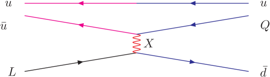
Figure 1: X boson exchange diagram giving the dimension 6 four fermion operator for proton and neutron decay.

4.2 Dimension 4 & 5 operators

The contribution of dimension 4 & 5 operators to nucleon decay in SUSY GUTs was noted by [Weinberg (1982); Sakai and Yanagida (1982)]. Dimension 4 operators are dangerous. In SUSY GUTs they always appear in the combination

$$(U^{c}\;D^{c}\;D^{c})+(Q\;L\;D^{c})+(E^{c}\;L\;L)$$ (44)

leading to unacceptable nucleon decay rates. R parity [Farrar and Fayet (1979)] forbids all dimension 3 and 4 (and even one dimension 5) baryon and lepton number violating operators. It is thus a necessary ingredient of any “natural” SUSY GUT.

Dimension 5 operators are obtained when integrating out heavy color triplet Higgs fields.

$$W\supset H_{u}\;QY_{u}\overline{U}+H_{d}(QY_{d}\overline{D}+LY_{e}\overline{E})+$$

$$T(Q{1\over 2}c_{qq}Q+\overline{U}c_{ue}\overline{E})+\bar{T}(Qc_{ql}L+\overline{U}c_{ud}\overline{D})$$

If the color triplet Higgs fields in Eqn. 4.2 {$T,\;\bar{T}$} have an effective mass term $M^{eff}_{T}\ \bar{T}\ T$ we obtain the dimension 5 operators

$$(1/M^{eff}_{T})\;\left[\ Q{1\over 2}c_{qq}Q\ Qc_{ql}L+\overline{U}c_{ud}\overline{D}\ \overline{U}c_{ue}\overline{E}\ \right],$$ (46)

denoted $LLLL$ and $RRRR$ operators, respectively. Nucleon decay via dimension 5 operators was considered by [Sakai and Yanagida (1982), Dimopoulos et al(1982), Ellis et al(1982)].

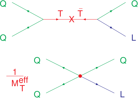
Figure 2: Color triplet Higgs exchange diagram giving the dimension 5 superpotential operator for proton and neutron decay.

The proton decay amplitude is then given generically by the expression

$$T(p\rightarrow K^{+}+\bar{\nu}) \propto\frac{c^{2}}{M^{eff}_{T}}\;({\rm Loop\;Factor)}\;(RG)\;\langle K^{+}\bar{\nu}|qqql|p\rangle$$

$$\sim\frac{c^{2}}{M^{eff}_{T}}\;{\rm(Loop\;Factor)}\;(RG)\;\frac{\beta_{lattice}}{f_{\pi}}\ m_{p}.$$

The last step used a chiral Lagrangian analysis to remove the $K^{+}$ state in favor of the vacuum state. Now we only need calculate the matrix element of a three quark operator between the proton and vacuum states. This defines the parameter $\beta_{lattice}$ using lattice QCD calculations. The decay amplitude includes four independent factors:

1. $\beta_{lattice}$, the three quark matrix element,

2. $c^{2}$, a product of two $3\times 3$ dimensionless coupling constant matrices,

3. a Loop Factor, which depends on the SUSY breaking squark, slepton and gaugino masses, and

4. $M^{eff}_{T}$, the effective color triplet Higgs mass which is subject to the GUT breaking sector of the theory.

Let us now consider each of these factors in detail.

4.2.1 $\beta_{lattice}$

The strong interaction matrix element of the relevant three quark operators taken between the nucleon and the appropriate pseudo-scalar meson may be obtained directly using lattice techniques. However these results have only been obtained recently [Aoki et al(JLQCD) (2000), Aoki et al(RBC) (2002)]. Alternatively, chiral Lagrangian techniques [Chadha et al(1983)] are used to replace the pseudo-scalar meson by the vacuum. Then the following three quark matrix elements are needed.

$$\beta U({\bf k})=\epsilon_{\alpha\beta\gamma}\smash{<}0|(u^{\alpha}d^{\beta})u^{\gamma}|{\rm proton}({\bf k})\smash{>},$$ (48)

$$\alpha U({\bf k})=\epsilon_{\alpha\beta\gamma}\smash{<}0|(\overline{\vphantom{d}u}^{*\,\alpha}\overline{d}^{*\,\beta})u^{\gamma}|{\rm proton}({\bf k})\smash{>}$$ (49)

and $U({\bf k})$ is the left handed component of the proton’s wavefunction. It has been known for some time that $|\beta|\approx|\alpha|$ [Brodsky et al(1984), Gavela et al(1989)] and that $|\beta|$ ranges from .003 to .03 GeV³ [Brodsky et al(1984), Hara et al(1986), Gavela et al(1989)]. Until quite recently, lattice calculations did not reduce the uncertainty in $|\beta|$; lattice calculations have reported $|\beta|$ as low as .006 GeV³ [Gavela et al(1989)] and as high as .03 GeV³ [Hara et al(1986)]. Additionally, the phase between $\alpha$ and $\beta$ satisfies $\beta\approx-\alpha$ [Gavela et al(1989)]. As a consequence, when calculating nucleon decay rates most authors have chosen to use a conservative lower bound with $|\alpha|\sim|\beta|=0.003$ GeV³ and an arbitrary relative phase.

Recent lattice calculations [Aoki et al(JLQCD) (2000), Aoki et al(RBC) (2002)] have obtained significantly improved results. In addition, they have compared the direct calculation of the three quark matrix element between the nucleon and pseudo-scalar meson to the indirect chiral Lagrangian analysis with the three quark matrix element between the nucleon and vacuum. [Aoki et al(JLQCD) (2000)] find

$$\beta_{lattice}=\langle 0|qqq|N\rangle=0.015(1)\;{\rm GeV}^{3}.$$ (50)

Also [Aoki et al(RBC) (2002)], in preliminary results reported in conference proceedings, obtained

$$\beta_{lattice}=0.007(1)\;{\rm GeV}^{3}.$$ (51)

They both find

$$\alpha_{lattice}\approx-\beta_{lattice}.$$ (52)

Several comments are in order. The previous theoretical range $0.003{\rm GeV}^{3}<\beta_{lattice}<0.03{\rm GeV}^{3}$ has been significantly reduced and the relative phase between $\alpha$ and $\beta$ has been confirmed. The JLQCD central value is 5 times larger than the previous “conservative lower bound.” Although the new, preliminary, RBC result is a factor of 2 smaller than that of JLQCD. We will have to wait for further results. What about the uncertainties? The error bars listed are only statistical. Systematic uncertainties (quenched + chiral Lagrangian) are likely to be of order $\pm 50$ % (my estimate). This stems from the fact that errors due to quenching are characteristically of order 30 %, while the comparison of the chiral Lagrangian results to the direct calculation of the decay amplitudes agree to within about 20 %, depending on the particular final state meson.

4.2.2 $c^{2}$ - Model Dependence

Consider the quark and lepton Yukawa couplings in SU(5) –

$$\lambda(\langle\Phi\rangle)\;10\;10\;5_{H}+\lambda^{\prime}(\langle\Phi\rangle)\;10\;\bar{5}\;\bar{5}_{H}$$ (53)

or in SO(10) –

$$\lambda(\langle\Phi\rangle)\;16\;16\;10_{H}.$$ (54)

The Yukawa couplings

$$\lambda(\langle\Phi\rangle),\;\;\lambda^{\prime}(\langle\Phi\rangle)$$ (55)

are effective higher dimensional operators, functions of adjoint ($\Phi$) (or higher dimensional) representations of SU(5) (or SO(10)). The adjoint representations are necessarily there in order to correct the unsuccessful predictions of minimal SU(5) (or SO(10)) and to generate a hierarchy of fermion masses. Once the adjoint (or higher dimensional) representations obtain VEVs ($\langle\Phi\rangle$), we find the Higgs Yukawa couplings –

$$H_{u}\;Q\ Y_{u}\ \overline{U}+H_{d}\ (\ Q\ Y_{d}\ \overline{D}+L\ Y_{e}\ \overline{E})$$ (56)

and also the effective dimension five operators

$$(1/M^{eff}_{T})\ \left[\ Q\ {1\over 2}c_{qq}\ Q\,Q\ c_{ql}\ L+\overline{U}\ c_{ud}\ \overline{D}\ \overline{U}\ c_{ue}\ \overline{E}\ \right].$$ (57)

Note, because of the Clebsch relations due to the VEVs of the adjoint representations, etc, we have

$$Y_{u}\neq c_{qq}\neq c_{ue}$$ (58)

and

$$Y_{d}\neq Y_{e}\neq c_{ud}\neq c_{ql}.$$ (59)

Hence, the $3\times 3$ complex matrices entering nucleon decay are not the same $3\times 3$ Yukawa matrices entering fermion masses. Is this complication absolutely necessary and how large can the difference be? Consider the SU(5) relation –

$$\lambda_{b}=\lambda_{\tau}$$ (60)

[Einhorn and Jones (1982), Inoue et al(1982), Ibañez and Lopez (1984)]. It is known to work quite well for small $\tan\beta\sim 1-2$ or large $\tan\beta\sim 50$ [Dimopoulos et al(1992), Barger et al(1993)]. For a recent discussion see [Barr and Dorsner (2003)]. On the other hand, the same relation for the first two families gives

$$\lambda_{s}=\lambda_{\mu}$$ (61)

$$\lambda_{d}=\lambda_{e}$$

leading to the unsuccessful relation

$$20\sim\frac{m_{s}}{m_{d}}=\frac{m_{\mu}}{m_{e}}\sim 200.$$ (62)

This bad relation can be corrected using Higgs multiplets in higher dimensional representations [Georgi and Jarlskog (1979), Georgi and Nanopoulos (1979), Harvey et al(1980,1982)] or using effective higher dimensional operators [Anderson et al(1994)]. Clearly the corrections to the simple SU(5) relation for Yukawa and c matrices can be an order of magnitude. Nevertheless, in predictive SUSY GUTs the c matrices are obtained once the fermion masses and mixing angles are fit [Kaplan and Schmaltz (1994), Babu and Mohapatra (1995), Lucas and Raby (1996), Frampton and Kong (1996), Blažek et al(1997), Barbieri and Hall (1997), Barbieri et al(1997), Allanach et al(1997), Berezhiani (1998), Blažek et al(1999,2000), Dermíšek and Raby (2000), Shafi and Tavartkiladze (2000), Albright and Barr (2000,2001), Altarelli et al(2000), Babu et al(2000), Berezhiani and Rossi (2001), Kitano and Mimura (2001), Maekawa (2001), King and Ross (2003), Chen and Mahanthappa (2003), Raby (2003), Ross and Velasco-Sevilla (2003), Goh et al(2003), Aulakh et al(2003)]. In spite of the above cautionary remarks we still find the inexact relations

$$c_{qq}\ c_{ql},\;\;c_{ud}\ c_{ue}\ \propto\ m_{u}\ m_{d}\ \tan\beta.$$ (63)

In addition, family symmetries can affect the texture of {$c_{qq},\ c_{ql},\ c_{ud},\ c_{ue}$}, just as it will affect the texture of Yukawa matrices.

In order to make predictions for nucleon decay it is necessary to follow these simple steps. Vary the GUT scale parameters, $\tilde{\alpha}_{G},\;M_{G}$, $Y_{u},\;Y_{d},\;Y_{e}$ and SOFT SUSY breaking parameters until one obtains a good fit to the precision electroweak data. Whereby we now explicitly include fermion masses and mixing angles in the category of precision data. Once these parameters are fit, then in any predictive SUSY GUT the matrices $c_{qq},\ c_{ql},\;c_{ud},\ c_{ue}$ at $M_{G}$ are also fixed. Now renormalize the dimension 5 baryon and lepton number violating operators from $M_{G}\rightarrow M_{Z}$ in the MSSM; evaluate the Loop Factor at $M_{Z}$ and renormalize the dimension 6 operators from $M_{Z}\rightarrow 1$ GeV. The latter determines the renormalization constant $A_{3}\sim 1.3$ [Dermíšek et al(2001)]. [Note, this should not be confused with the renormalization factor $A_{L}\sim.22$ [Ellis et al(1982)] which is used when one does not have a theory for Yukawa matrices. The latter RG factor, takes into account the combined renormalization of the dimension 6 operator from the weak scale to 1 GeV and also the renormalization of fermion masses from 1 GeV to the weak scale.] Finally calculate decay amplitudes using a chiral Lagrangian approach or direct lattice gauge calculation.

Before leaving this section we should remark that we have assumed that the electroweak Higgs in SO(10) models is contained solely in a 10. If however the electroweak Higgs is a mixture of weak doublets from $16_{H},\;10_{H}$ and, in addition, we include the higher dimensional operator $\frac{1}{M}(16\ 16\ 16_{H}\ 16_{H})$, useful for neutrino masses, then there are additional contributions to the dimension 5 operators considered in (Eqn. 46) [Babu et al(2000)]. However these additional terms are not required for neutrino masses [Blažek et al(1999,2000)].

4.3 Loop factor

The dimension 5 operators are a product of two fermion and two scalar fields. The scalar squarks and/or sleptons must be integrated out of the theory below the SUSY breaking scale. There is no consensus on the best choice for an appropriate SUSY breaking scale. Moreover, in many cases there is a hierarchy of SUSY particle masses. Hence we take the simplest assumption, integrating out all SUSY particles at $M_{Z}$. When integrating out the SUSY particles in loops, the effective dimension 5 operators are converted to effective dimension 6 operators. This results in a loop factor which depends on the sparticle masses and mixing angles.

Consider the contribution to the loop factor for the process $p\rightarrow K^{+}+\bar{\nu}_{\tau}$ in Fig. 3. This graph is due to the RRRR operators and gives the dominant contribution at large $\tan\beta$ and a significant contribution for all values of $\tan\beta$ [Lucas and Raby (1997), Babu and Strassler (1998), Goto and Nihei (1999), Murayama and Pierce (2002)].

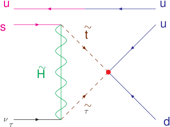
Figure 3: Higgsino and third generation stop - stau loop giving the dominant loop contribution to dimension 5 nucleon decay.

Although the loop factor is a complicated function of the sparticle masses and mixing angles, it nevertheless has the following simple dependence on the overall gaugino and scalar masses given by

$$\frac{\lambda_{t}\;\lambda_{\tau}}{16\pi^{2}}\frac{\sqrt{\mu^{2}+M_{1/2}^{2}}}{m_{16}^{2}}.$$ (64)

Thus in order to minimize this factor one needs

$$\mu,\;M_{1/2}\;\;\;{\rm SMALL}$$ (65)

and

$$m_{16}\;\;\;{\rm Large}.$$ (66)

4.4 $M_{t}^{eff}$

The largest uncertainty in the nucleon decay rate is due to the color triplet Higgs mass parameter $M^{eff}_{T}$. As $M^{eff}_{T}$ increases, the nucleon lifetime increases. Thus it is useful to obtain an upper bound on the value of $M^{eff}_{T}$. This constraint comes from imposing perturbative gauge coupling unification [Lucas and Raby (1997), Goto and Nihei (1999), Babu et al(2000), Altarelli et al(2000), Dermíšek et al(2001), Murayama and Pierce (2002)]. Recall, in order to fit the low energy data a GUT scale threshold correction

$$\epsilon_{3}\equiv\frac{(\alpha_{3}(M_{G})-\tilde{\alpha}_{G})}{\tilde{\alpha}_{G}}\sim-3\%\;\;{\rm to}\;-4\%$$ (67)

is needed. $\epsilon_{3}$ is a logarithmic function of particle masses of order $M_{G}$, with contributions from the electroweak Higgs and GUT breaking sectors of the theory.

$$\epsilon_{3}= \epsilon_{3}^{\rm Higgs}+\epsilon_{3}^{\rm GUT\;breaking}+\cdots,$$ (68)

$$\epsilon_{3}^{\rm Higgs}= \frac{3\alpha_{G}}{5\pi}\ln(\frac{M^{eff}_{T}}{M_{G}}).$$ (69)

In Table 3 we have analyzed three different GUT theories – the minimal SU(5) model, an SU(5) model with natural doublet-triplet splitting and minimal SO(10) (which also has natural doublet-triplet splitting). We have assumed that the low energy data, including weak scale threshold corrections, requires $\epsilon_{3}=-4\%$. We have then calculated the contribution to $\epsilon_{3}$ from the GUT breaking sector of the theory in each case.

Minimal SU(5) is defined by its minimal GUT breaking sector with one SU(5) adjoint $\Sigma$. The one loop contribution from this sector to $\epsilon_{3}$ vanishes. Hence, the $-4$ % must come from the Higgs sector alone, requiring the color triplet Higgs mass $M^{eff}_{T}\sim 2\times 10^{14}$ GeV. Note since the Higgs sector is also minimal, with the doublet masses fine-tuned to vanish, we have $M^{eff}_{T}\equiv M_{T}$. By varying the SUSY spectrum at the weak scale, we may be able to increase $\epsilon_{3}$ to $-3$ % or even $-2$ %, but this cannot save minimal SU(5) from disaster due to rapid proton decay from Higgsino exchange.

In the other theories, Higgs doublet - triplet splitting is obtained without fine-tuning. This has two significant consequences. First, the GUT breaking sectors are more complicated, leading in these theories to large negative contributions to $\epsilon_{3}$. The maximum value $|\epsilon_{3}|\sim 10\%$ in minimal SO(10) is fixed by perturbativity bounds [Dermíšek et al(2001)]. Secondly, the effective color triplet Higgs mass $M^{eff}_{T}$ does not correspond to the mass of any particle in the theory. In fact, in both cases with “natural” doublet-triplet splitting, the color triplet Higgs mass is of order $M_{G}$ even though $M^{eff}_{T}\gg M_{G}$. The values for $M^{eff}_{T}$ in Table 3 are fixed by the value of $\epsilon_{3}^{\rm Higgs}$ needed to obtain $\epsilon_{3}=-4\%$.

Table 3: GUT threshold corrections in three different theories. The first column is the minimal SU(5) SUSY theory [Dimopoulos and Georgi (1981) Sakai (1982), Goto and Nihei (1999), Murayama and Pierce (2002)], the second column is SU(5) with “natural” Higgs doublet-triplet splitting [Masiero et al(1982), Grinstein (1982), Altarelli et al(2000)], and the third column is minimal SO(10) SUSY model [Blažek et al(1999.2000), Dermíšek et al(2001), Blažek et al(2002a,b)].

• 	Minimal SU(5)	SU(5) “Natural” D/T	Minimal SO(10)
  $\epsilon_{3}^{\rm GUTbreaking}$	0	- 7.7 %	- 10 %
  $\epsilon_{3}^{\rm Higgs}$	- 4 %	+ 3.7 %	+ 6 %
  $M^{eff}_{T}\;{\rm[GeV]}$	$2\times 10^{14}$	$3\times 10^{18}$	$6\times 10^{19}$

Before discussing the bounds on the proton lifetime due to the exchange of color triplet Higgsinos, let us elaborate on the meaning of $M^{eff}_{T}$. Consider a simple case with two pairs of SU(5) Higgs multiplets, { $\bar{5}_{H}^{i},\;\;5_{H}^{i}$ } with $i=1,2$. In addition, also assume that only { $\bar{5}_{H}^{1},\;\;5_{H}^{1}$ } couples to quarks and leptons. Then $M^{eff}_{T}$ is defined by the expression

$$\frac{1}{M^{eff}_{T}}=(M_{T}^{-1})_{11}$$ (70)

where $M_{T}$ is the color triplet Higgs mass matrix. In the cases with “natural” doublet - triplet splitting, we have

$$M_{T}=\left(\begin{array}[]{cc}0&M_{G}\\ M_{G}&X\end{array}\right)$$ (71)

with

$$\frac{1}{M^{eff}_{T}}\equiv\frac{X}{M_{G}^{2}}.$$ (72)

Thus for $X\ll M_{G}$ we have $M^{eff}_{T}\gg M_{G}$ and no particle has mass greater than $M_{G}$ [Babu and Barr (1993)]. The large Higgs contribution to the GUT threshold correction is in fact due to an extra pair of light Higgs doublets with mass of order $X$.

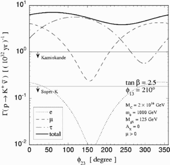
Figure 4: [Fig. 2: Goto and Nihei (1999)] Decay rates $\Gamma(p\rightarrow K^{+}\bar{\nu}_{i})\;(i=e,\mu\;{\rm and}\;\tau)$ as functions of the phase $\phi_{23}$ for $\tan\beta=2.5$. The soft SUSY breaking parameters are fixed at $m_{0}=1$ TeV, $M_{\tilde{g}}=125$ GeV and $A_{0}=0$ with $\mu>0$. $M_{T}$ and $M_{\Sigma}$ are taken as $M_{T}=M_{\Sigma}=2\times 10^{16}$ GeV. The horizontal lower line corresponds to the Super-Kamiokande limit $\tau(p\rightarrow K^{+}\bar{\nu})>5.5\times 10^{32}$ years, and the horizontal upper line corresponds to the Kamiokande limit $\tau(p\rightarrow K^{+}\bar{\nu})>1.0\times 10^{32}$ years. The new Super-Kamiokande bound is $\tau(p\rightarrow K^{+}\bar{\nu})>1.9\times 10^{33}$ years.

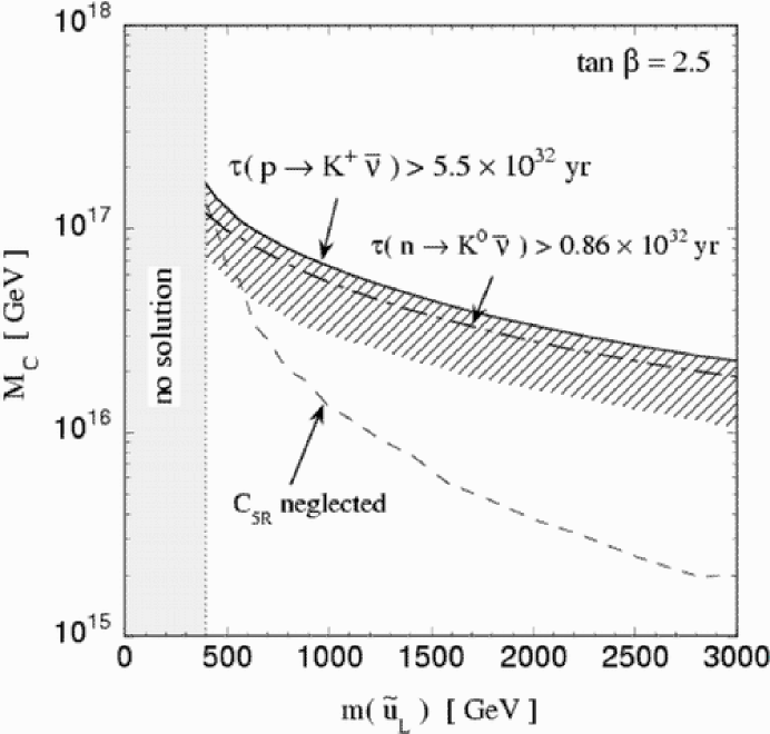
Figure 5: [Fig. 4: Goto and Nihei (1999)] Lower bound on the colored Higgs mass $M_{T}$ as a function of the left-handed scalar up quark mass $m_{\tilde{u}_{L}}$. The soft SUSY breaking parameters $m_{0},\;M_{\tilde{g}},\;A_{0}$ are scanned within the range $0<m_{0}<3$ TeV, $0<M_{\tilde{g}}<1$ TeV and $-5<A_{0}<5$ with $\tan\beta$ fixed at 2.5. Both signs of $\mu$ are considered. The whole parameter region of the two phases $\phi_{13}$ and $\phi_{23}$ is examined. The solid curve represents the bound derived from the Super-Kamiokande limit $\tau(p\rightarrow K^{+}\bar{\nu})>5.5\times 10^{32}$ years and the dashed curve represents the corresponding result without the RRRR effect. The left-hand side of the vertical dotted line is excluded by other experimental constraints. The dash-dotted curve represents the bound derived from the Kamiokande limit on the neutron partial lifetime $\tau(n\rightarrow K^{0}\bar{\nu})>0.86\times 10^{32}$ years.

Due to the light color triplet Higgsino, it has been shown that minimal SUSY SU(5) is ruled out by the combination of proton decay constrained by gauge coupling unification [Goto and Nihei (1999), Murayama and Pierce (2002)] !! In Figs. 4 and 5 we reprint the figures from the paper by [Goto and Nihei (1999)]. In Fig. 4 the decay rate for $p\rightarrow K^{+}\bar{\nu}_{i}$ for any one of the three neutrinos $(i=e,\mu\;{\rm and}\;\tau)$ is plotted for fixed soft SUSY breaking parameters as a function of the relative phase $\phi_{23}$ between two LLLL contributions to the decay amplitude. The phase $\phi_{13}$ is the relative phase between one of the LLLL contributions and the RRRR contribution. The latter contributes predominantly to the $\bar{\nu}_{\tau}$ final state, since it is proportional to the up quark and charged lepton Yukawa couplings. As noted by [Goto and Nihei (1999)], the partial cancellation between LLLL contributions to the decay rate is completely filled by the RRRR contribution. It is this result which provides the stringent limit on minimal SUSY SU(5). As one sees from Fig. 4, for the color triplet Higgs mass $M_{T}=2\times 10^{16}$ GeV ($\equiv M_{C}$ in the notation of [Goto and Nihei (1999)]), the universal scalar mass $m_{0}=$ 1 TeV and $\tan\beta=2.5$, there is no value of the phase $\phi_{23}$ which is consistent with Super-Kamiokande bounds. Note, the proton decay rate scales as $\tan\beta^{2}$; hence the disagreement with data only gets worse as $\tan\beta$ increases. In Fig. 5 the contour of constant proton lifetime is plotted in the $M_{T}(\equiv M_{C})$ – $m(\tilde{u}_{L})$ plane, where $m(\tilde{u}_{L})$ is the mass of the left-handed up squark for $\tan\beta=2.5$. Again, there is no value of $m(\tilde{u}_{L})<3$ TeV for which the color triplet Higgs mass is consistent with gauge coupling unification. In [Goto and Nihei (1999)] the up squark mass was increased by increasing $m_{0}$. Hence all squarks and slepton masses increased.

One may ask whether one can suppress the proton decay rate by increasing the mass of the squarks and sleptons of the first and second generation, while keeping the third generation squarks and sleptons light (in order to preserve “naturalness”). This is the question addressed by [Murayama and Pierce (2002)]. They took the first and second generation scalar masses of order 10 TeV, with the third generation scalar masses less than 1 TeV. They showed that since the RRRR contribution does not decouple in this limit, and moreover since any possible cancellation between the LLLL and RRRR diagrams vanishes in this limit, one finds that minimal SUSY SU(5) cannot be saved by decoupling the first two generations of squarks and sleptons.

Thus minimal SUSY SU(5) is dead. Is this something we should be concerned about. In my opinion, the answer is no, although others may disagree [Bajc et al(2002)]. Minimal SUSY SU(5) has two a priori unsatisfactory features:

• It requires fine-tuning for Higgs doublet-triplet splitting, and

• renormalizable Yukawa couplings due to $5_{H},\;\bar{5}_{H}$ alone are not consistent with fermion masses and mixing angles.

Thus it was clear from the beginning that two crucial ingredients of a realistic theory were missing. The theories which work much better have “natural” doublet-triplet splitting and fit fermion masses and mixing angles.

4.5 Summary of Nucleon Decay in 4D

Minimal SUSY SU(5) is excluded by the concordance of experimental bounds on proton decay and gauge coupling unification. We discussed the different factors entering the proton decay amplitude due to dimension 5 operators.

$$T(p\rightarrow K^{+}+\bar{\nu})\sim\frac{c^{2}}{M^{eff}_{T}}{\rm(Loop\;Factor)}\;\frac{\beta_{lattice}}{f_{\pi}}\ m_{p}.$$ (73)

We find

• $c^{2}$: model dependent but constrained by fermion masses and mixing angles;

• $\beta_{lattice}$: JLQCD central value is 5 times larger than the previous “conservative lower bound.” However one still needs to reduce the systematic uncertainties of quenching and chiral Lagrangian analyses. Moreover, the new RBC result is a factor of 2 smaller than JLQCD;

• Loop Factor: $\propto\frac{\lambda_{t}\ \lambda_{\tau}}{16\pi^{2}}\frac{\sqrt{\mu^{2}+M_{1/2}^{2}}}{m_{16}^{2}}$. It is minimized by taking gauginos light and the 1st and 2nd generation squarks and sleptons heavy ($>$ TeV). However, “naturalness” requires that the stop, sbottom and stau masses remain less than of order 1 TeV;

• $M^{eff}_{T}$: constrained by gauge coupling unification and GUT breaking sectors.

The bottom line we find for dimension 6 operators [Lucas and Raby (1997), Murayama and Pierce (2002)]

$$\tau_{(}p\rightarrow\pi^{0}+e^{+})\approx 5\times 10^{36}\;(\frac{M_{X}}{3\times 10^{16}\ {\rm GeV}})^{4}\;(\frac{0.015\ {\rm GeV}^{3}}{\beta_{lattice}})^{2}\;\;{\rm years}.$$ (74)

Note, it has been recently shown [Klebanov and Witten (2003)] that string theory can possibly provide a small enhancement of the dimension 6 operators. Unfortunately the enhancement is very small. Thus it is very unlikely that these dimension 6 decay modes $p\rightarrow\pi^{0}+e^{+}$ will be observed.

On the other hand for dimension 5 operators in realistic SUSY GUTs we obtain rough upper bounds on the proton lifetime coming from gauge coupling unification and perturbativity [Babu et al(2000), Altarelli et al(2000), Dermíšek et al(2001)]

$$\tau(p\rightarrow K^{+}+\bar{\nu})<(\frac{1}{3}-3)\times 10^{34}\;(\frac{0.015\ {\rm GeV}^{3}}{\beta_{lattice}})^{2}\;\;{\rm years}.$$ (75)

Note in general

$$\tau(n\rightarrow K^{0}+\bar{\nu})<\tau(p\rightarrow K^{+}+\bar{\nu}).$$ (76)

Moreover other decay modes may be significant, but they are very model dependent, for example [Carone et al(1996), Babu et al(2000)]

$$p\rightarrow\pi^{0}+e^{+},\;\;K^{0}+\mu^{+}.$$ (77)

4.6 Proton decay in more than four dimensions

We should mention that there has been a recent flurry of activity on SUSY GUTs in extra dimensions beginning with the work of [Kawamura (2001a,b)]. However the study of extra dimensions on orbifolds goes back to the original work of [Dixon et al(1985,1986)] in string theory. Although this interesting topic would require another review, let me just mention some pertinent features here. In these scenarios, grand unification is only a symmetry in extra dimensions which are then compactified at scales of order $1/M_{G}$. The effective four dimensional theory, obtained by orbifolding the extra dimensions, has only the standard model gauge symmetry or at most a Pati-Salam symmetry which is then broken by the standard Higgs mechanism. In these theories, it is possible to completely eliminate the contribution of dimension 5 operators to nucleon decay. This may be a consequence of global symmetries as shown by [Witten (2002), Dine et al(2002)] or a continuous U(1)_R symmetry (with R parity a discrete subgroup)[Hall and Nomura (2002)]. [Note, it is also possible to eliminate the contribution of dimension 5 operators in 4 dimensional theories with extra symmetries [Babu and Barr (2002)], but these 4 dimensional theories are quite convoluted. Thus it is difficult to imagine that nature takes this route. On the other hand, in one or more small extra dimensions the elimination of dimension 5 operators is very natural.] Thus at first glance, nucleon decay in these theories may be extremely difficult to see. However this is not necessarily the case. Once again we must consider the consequences of grand unification in extra dimensions and gauge coupling unification.

Extra dimensional theories are non-renormalizable and therefore require an explicit cutoff scale $M_{*}$, assumed to be larger than the compactification scale $M_{c}$. The Kałuza-Klein excitations above $M_{c}$ contribute to threshold corrections to gauge coupling unification evaluated at the compactification scale. The one loop renormalization of gauge couplings is given by

$$\frac{2\pi}{\alpha_{i}(\mu)} = \frac{2\pi}{\alpha(M_{*})}+b_{i}\log(\frac{M_{c}}{\mu})+\Delta_{i}$$ (78)

where $\Delta_{i}$ are the threshold corrections due to all the KK modes from $M_{c}$ to $M_{*}$ and can be expressed as $\Delta_{i}=b^{eff}_{i}\log(\frac{M_{*}}{M_{c}})$ [Hall and Nomura (2001,2002a), Nomura et al(2001), Contino et al(2002), Nomura (2002)]. In a 5D SO(10) model, broken to Pati-Salam by orbifolding and to the MSSM via Higgs VEVs on the brane, it was shown [Kim and Raby (2003)] that the KK threshold corrections take a particularly simple form

$$\frac{2\pi}{\alpha_{i}(\mu)} = \frac{2\pi}{\alpha(M_{*})}+b^{MSSM}_{i}\log(\frac{\hat{M}_{c}}{\mu})+\hat{\Delta}_{i}$$ (79)

$$= \frac{2\pi}{\alpha(M_{*})}+b^{MSSM}_{i}\log(\frac{\hat{M}_{c}}{\mu})+\frac{2}{3}b^{SM}_{i}(V)\log(\frac{M_{*}}{\hat{M}_{c}}).$$ (80)

with

$$\hat{\Delta}_{\rm gauge} = \frac{2}{3}b^{SM}_{i}(V)\log(\frac{M_{*}}{\hat{M}_{c}})$$ (81)

$$\hat{\Delta}_{Higgs} = 0,$$ (82)

and $\hat{M}_{c}\equiv(\pi R/2)^{-1}$. Here $b^{MSSM}$ includes the gauge sector and the Higgs sector together and $b^{SM}(V)$ includes the gauge sector only. The running equation is very simple and permits us to directly compare with well known 4D SUSY GUTs. In the minimal 4D SU(5) SUSY model, the running equation is given by

$$\frac{2\pi}{\alpha_{i}(\mu)} = \frac{2\pi}{\alpha(M_{GUT})}+b^{MSSM}_{i}\log(\frac{M_{T}}{\mu})+b^{SM}_{i}(V)\log(\frac{M_{GUT}}{M_{T}}).$$ (83)

where $M_{T}$ is the color triplet Higgs mass. As discussed earlier, we can achieve unification by adjusting the color triplet Higgs mass $M_{T}=2\times 10^{14}\,{\rm GeV}$ (see Table 3).

Comparing Eqn. (80) and (83), we observe that if

$$\hat{M}_{c}=M_{T},\,\,\,\,\,\frac{M_{*}}{\hat{M}_{c}}=(\frac{M_{GUT}}{M_{T}})^{\frac{3}{2}},$$

the same unification is achieved here. Therefore we get $\hat{M}_{c}=2\times 10^{14}\,{\rm GeV}$ and $M_{*}=3.7\times 10^{17}\,{\rm GeV}$ by using $M_{GUT}=3\times 10^{16}\,{\rm GeV}$. A few remarks are in order. There is no problem with proton decay due to dimension 5 operators, even though the color triplet Higgs mass is of order $10^{14}\,{\rm GeV}$, since these operators are excluded by R symmetry. In a 5D model, the 4D GUT scale has no fundamental significance. The couplings unify at the cutoff scale and there is no scale, above which we have a perturbative SO(10) GUT.

In Fig. 6 we show the running in the difference of couplings for two independent cases.

1. We show the couplings for four dimensional gauge theories with GUT scale thresholds, in which the GUT scale is defined as the point where $\alpha_{1}$ and $\alpha_{2}$ meet and $\epsilon_{3}$ is the relative shift in $\alpha_{3}$ due to threshold corrections, and

2. for a five dimensional SO(10) model where the three couplings meet at the cutoff scale and the threshold corrections due to the KK tower is defined at the compactification scale.

In both cases, the running of the gauge couplings below the compactification scale must be the same. Thus we can use the low energy fits from 4D theories to constrain a 5D theory.

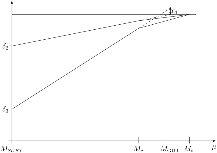
Figure 6: Differential running of $\delta_{2}=2\pi(\frac{1}{\alpha_{2}}-\frac{1}{\alpha_{1}})$ and $\delta_{3}=2\pi(\frac{1}{\alpha_{3}}-\frac{1}{\alpha_{1}})$.

Note, since the the KK modes of the baryon number violating {$X,\ \bar{X}$} gauge bosons have mass starting at the compactification scale $M_{c}\approx 10^{14}\,{\rm GeV}$ we must worry whether proton decay due to dimension 6 operators is safe. It has been shown [Altarelli and Feruglio (2001), Hall and Nomura (2002b), Hebecker and March-Russell (2002)] that this depends on where in the extra dimensions the quarks and leptons reside. If they are on symmetric orbifold fixed points, i.e. symmetric under the GUT symmetry, then this leads to the standard dimension 6 proton decay operators which is ruled out for the first and second families of quarks and leptons. Hence the first two families must be either in the bulk or on broken symmetry fixed points. If they are in the bulk, then the {$X,\ \bar{X}$} mediated processes take massless modes to KK excitations which is not a problem. Otherwise, if the first two families are on the broken symmetry fixed point, the wave functions for the {$X,\ \bar{X}$} bosons vanish there. However, certain effective higher dimensional operators on the broken symmetry orbifold fixed points can allow the {$X,\ \bar{X}$} bosons to couple to the first two families. These operators are allowed by symmetries and they naturally lead to proton lifetimes for $p\rightarrow e^{+}\ \pi^{0}$ of order $10^{34\pm 2}$ years. The large uncertainty is due to the order of magnitude uncertainty in the coefficient of these new effective operators.

Before closing this section, we should make a few comments on theories with large extra dimensions of order 1/TeV or as large as 1 mm. In some of these theories, only gravity lives in higher dimensions while the ordinary matter and gauge interactions typically reside on a three dimensional brane [Arkani-Hamed et al(1998)]. While if the extra dimensions are no larger than 1/TeV, all matter may live in the bulk. Such theories replace SUSY with new and fundamental non-perturbative physics at the 1 - 10 TeV scale. These theories must address the question of why dimension 6 proton decay operators, suppressed only by 1/TeV², are not generated. There are several ideas in the literature with suggested resolutions to this problem. They include:

• conserved baryon number on the brane with anomaly cancelling Chern-Simons terms in the bulk,

• or displacing quarks from leptons on a “fat” brane with a gaussian suppression of the overlap of the quark/lepton wave functions.

A novel solution to the problem of proton decay is found in 6 space-time dimensional theories with all matter spanning the two extra dimensions. It has been shown that in such theories [Appelquist et al(2001)] a Z(8) remnant of the 6 dimensional Lorentz group is sufficient to suppress proton decay to acceptable levels. These theories predict very high dimensional proton decay operators with multi-particle final states.

5 Fermion masses and mixing

Low energy SUSY provides a natural framework for solving the gauge hierarchy problem, while SUSY GUTs make the successful prediction for gauge coupling unification and the, still un-verified, prediction for proton decay. But these successes affect only a small subset of the unexplained arbitrary parameters in the standard model having to do with the Z and Higgs masses (i.e. the weak scale) and the three gauge coupling constants. On the other hand, the sector of the standard model with the largest number of arbitrary parameters has to do with fermion masses and mixing angles. Grand unification also provides a natural framework for discussing the problem of fermion masses, since it naturally arranges quarks and leptons into a few irreducible multiplets, thus explaining their peculiar pattern of gauge charges, i.e. charge quantization and the family structure. Moreover, it has been realized for some time that the masses and mixing angles of quarks and leptons are ordered with respect to their generation (or family) number. The first generation of quarks and leptons, {$u,\ d,\ e,\ \nu_{e}$}, are the lightest; the second generation, {$c,\ s,\ \mu,\ \nu_{\mu}$}, are all heavier than the first, and the third generation, {$t,\ b,\ \tau,\ \nu_{\tau}$}, are the heaviest (see Table 4).

Table 4: Quark and lepton masses in units of MeV/c².

• 	$\nu_{e}$	e	u	d
  1st	$\leq 10^{-7}$	1/2	2	5
  2nd	$\leq 10^{-7}$	105.6	1,300	120
  3rd	$\leq 10^{-7}$	1,777	174,000	4,500

In addition, the first two generations have a weak mixing angle given by the Cabibbo angle, $\theta_{C}$. If we define $\lambda\equiv\sin\theta_{C}\sim.22$, then the mixing of the second and third generation is of order $\lambda^{2}$ and the first and third is the weakest mixing of order $\lambda^{3}$. This pattern is very elegantly captured in the Wolfenstein representation of the CKM matrix given by

$$V_{CKM} =\left(\begin{array}[]{ccc}V_{ud}&V_{us}&V_{ub}\\ V_{cd}&V_{cs}&V_{cb}\\ V_{td}&V_{ts}&V_{tb}\end{array}\right)$$ (87)

$$\approx\left(\begin{array}[]{ccc}1-\frac{1}{2}\lambda^{2}&\lambda&(\rho-i\eta)\ A\ \lambda^{3}\\ -\lambda&1-\frac{1}{2}\lambda^{2}&A\ \lambda^{2}\\ (1-\rho-i\eta)\ A\ \lambda^{3}&-A\ \lambda^{2}&1\end{array}\right)$$ (91)

with $\lambda\sim 1/5$, $\;A\sim 1$ and $|\rho-i\eta|\sim 1/2$.

Although the fundamental explanation for three families is still wanting, it is natural to assume that the families transform under some family symmetry. Such a possibility is consistent with weakly coupled heterotic string theory where, for example, $E(8)\times E(8)$ and SO(32) are both large enough to contain a GUT group $\times$ a family symmetry. Such a family symmetry has many potential virtues.

• A spontaneously broken family symmetry can explain the hierarchy of fermion masses and mixing angles.

• In a SUSY theory, the family symmetry acts on both fermions and sfermions, thus aligning the quark and squark, and the lepton and slepton mass matrices. This suppresses flavor violating processes.

• The combination of a family and a GUT symmetry can reduce the number of fundamental parameters in the theory, hence allowing for a predictive theory.

In the following sections, we consider several important issues. In section 5.1 we discuss the simplest case of the third generation only. Here we discuss the status of SU(5) ($\lambda_{b}=\lambda_{\tau}$) and SO(10) ($\lambda_{t}=\lambda_{b}=\lambda_{\tau}=\lambda_{\nu_{\tau}}$) Yukawa unification. In section 5.2 we consider several different analyses in the literature for three family models with either U(1) or non-abelian family symmetry. In section 5.3 we study the relation between charged fermion and neutrino masses in SUSY GUTs and consider some examples giving bi-large neutrino mixing consistent with the data. Finally, in section 5.4 we discuss some experimental consequences of SUSY theories of fermion masses. In particular, we consider $b\rightarrow s\gamma$, $(g-2)_{\mu}$, $B_{s}\rightarrow\mu^{+}\ \mu^{-}$, $\mu\rightarrow e\gamma$ and the electric dipole moments $d_{n},\ d_{e}$.

5.1 Yukawa unification

Let us first discuss the most stringent case of SO(10) Yukawa unification. It has been shown [Raby (2001), Dermíšek (2001), Baer and Ferrandis (2001), Blažek et al(2002a,b), Auto et al(2003), Tobe and Wells (2003)] that SO(10) boundary conditions at the GUT scale, for soft SUSY breaking parameters as well as for the Yukawa couplings of the third generation, are consistent with the low energy data, including $M_{t},\ m_{b}(m_{b}),\ M_{\tau}$, ONLY in a narrow region of SUSY breaking parameter space. Moreover, this region is also preferred by constraints from CP and flavor violation, as well as by the non-observation of proton decay. Finally we discuss the consequences for the Higgs and SUSY spectrum.

Recall, in SO(10) we have the compelling unification of all quarks and leptons of one family into one irreducible representation such that ${\bf 10}+{\bf\bar{5}}+\bar{\nu}_{sterile}\ \subset\ {\bf 16}$ and the two Higgs doublets are also unified with ${\bf 5_{H}},\;{\bf\bar{5}_{H}}\ \subset\ {\bf 10_{H}}$. Hence, minimal SO(10) also predicts Yukawa unification for the third family of quarks and leptons with $\lambda_{b}=\lambda_{t}=\lambda_{\tau}=\lambda_{\nu_{\tau}}=\lambda$ at the GUT scale [Banks (1988), Olechowski and Pokorski (1988), Pokorski (1990), Shafi and Ananthanarayan (1991);Ananthanarayan et al(1991,1993,1994), Anderson et al(1993,1994)].

Ignoring threshold corrections, one can use the low energy value for $m_{b}/m_{\tau}$ to fix the universal Yukawa coupling $\lambda$. RG running from $M_{G}$ to $M_{Z}$ then gives $\lambda_{\tau}(M_{Z})$. Then given $m_{\tau}=\lambda_{\tau}\frac{v}{\sqrt{2}}cos\beta$ we obtain $\tan\beta\approx 50$. Finally, a prediction for the top quark mass is given with $m_{t}=\lambda_{t}\frac{v}{\sqrt{2}}sin\beta\sim 170\pm 20\;{\rm GeV}$ (see [Anderson et al(1993)]).

Note, in this case there are insignificant GUT threshold corrections from gauge and Higgs loops. Nevertheless, the previous discussion is essentially a straw man, since there are huge threshold corrections at the weak scale [Hall et al(1994), Hempfling (1994), Carena et al(1994), Blažek et al(1995)]. The dominant contributions are from gluino and chargino loops plus an overall logarithmic contribution due to finite wave function renormalization given by $\delta m_{b}/m_{b}=\Delta m_{b}^{\tilde{g}}+\Delta m_{b}^{\tilde{\chi}}+\Delta m_{b}^{\log}+\cdots$ (see Fig. 7). These contributions are approximately of the form

$$\Delta m_{b}^{\tilde{g}}\approx\frac{2\alpha_{3}}{3\pi}\;\frac{\mu m_{\tilde{g}}}{m_{\tilde{b}}^{2}}\;tan\beta,$$ (92)

$$\Delta m_{b}^{\tilde{\chi}^{+}}\approx\frac{\lambda_{t}^{2}}{16\pi^{2}}\;\frac{\mu A_{t}}{m_{\tilde{t}}^{2}}\;tan\beta\;\;\;{\rm and}$$ (93)

$$\Delta m_{b}^{\log}\approx\frac{\alpha_{3}}{4\pi}\log(\frac{\tilde{m}^{2}}{M_{Z}^{2}})\sim 6\%$$ (94)

with $\Delta m_{b}^{\tilde{g}}\sim-\Delta m_{b}^{\tilde{\chi}}>0$ for $\mu>0$ [with our conventions]. These corrections can easily be of order $\sim 50$ %. However good fits require $-4\%<\delta m_{b}/m_{b}<-2\%$.

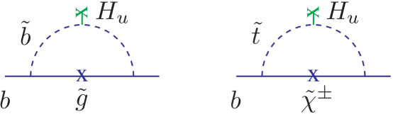
Figure 7: The one loop gluino (left) and chargino (right) corrections to the bottom quark mass proportional to $\alpha_{s}$ (left) and $\lambda_{t}$ (right) and to $\tan\beta$.

Note, the data favors $\mu>0$. First consider the process $b\rightarrow s\gamma$. The chargino loop contribution typically dominates and has opposite sign to the standard model and charged Higgs contributions for $\mu>0$, thus reducing the branching ratio. This is desirable, since the standard model contribution is a little too large. Hence $\mu<0$ is problematic when trying to fit the data. Secondly, the recent measurement of the anomalous magnetic moment of the muon suggests a contribution due to NEW physics given by $a_{\mu}^{NEW}=22.1(11.3)\times 10^{-10}$ or $7.4(10.5)\times 10^{-10}$ [Muon g - 2 Collaboration (2002), Davier et al(2003)] depending on whether one uses $e^{+}e^{-}$ or $\tau$ hadronic decay data to evaluate the leading order hadronic contributions. For other recent theoretical analyses and references to previous work see [Hagiwara et al(2003), Melnikov and Vainshtein (2003)]. However in SUSY the sign of $a_{\mu}^{NEW}$ is correlated with the sign of $\mu$ [Chattopadhyay and Nath (1996)]. Once again the data favors $\mu>0$.

Before discussing the analysis of Yukawa unification, specifically that of [Blažek et al(2002a,b)], we need to consider one important point. $SO(10)$ Yukawa unification with the minimal Higgs sector necessarily predicts large $\tan\beta\sim 50$. In addition, it is much easier to obtain EWSB with large $\tan\beta$ when the Higgs up/down masses are split ($m_{H_{u}}^{2}<m_{H_{d}}^{2}$) [Olechowski and Pokorski (1995), Matalliotakis and Nilles (1995), Polonsky and Pomarol (1995), Murayama, Olechowski and Pokorski (1996), Rattazzi and Sarid (1996)]. In the following analysis we consider two particular Higgs splitting schemes we refer to as Just So and D term splitting. In the first case the third generation squark and slepton soft masses are given by the universal mass parameter $m_{16}$, and only Higgs masses are split: $m_{(H_{u},\;H_{d})}^{2}=m_{10}^{2}\;(1\mp\Delta m_{H}^{2})$. In the second case we assume D term splitting, i.e. that the D term for $U(1)_{X}$ is non-zero, where $U(1)_{X}$ is obtained in the decomposition of $SO(10)\rightarrow SU(5)\times U(1)_{X}$. In this second case, we have $m_{(H_{u},\;H_{d})}^{2}=m_{10}^{2}\mp 2D_{X}$, $m_{(Q,\;\bar{u},\;\bar{e})}^{2}=m_{16}^{2}+D_{X}$, $m_{(\bar{d},\;L)}^{2}=m_{16}^{2}-3D_{X}$. The Just So case does not at first sight appear to be very well motivated. However we now argue that it is quite natural [Blažek et al(2002a,b)]. In $SO(10)$, neutrinos necessarily have a Yukawa term coupling active neutrinos to the “sterile” neutrinos present in the 16. In fact for $\nu_{\tau}$ we have $\lambda_{\nu_{\tau}}\;\bar{\nu}_{\tau}\;L\;H_{u}$ with $\lambda_{\nu_{\tau}}=\lambda_{t}=\lambda_{b}=\lambda_{\tau}\equiv\;{\bf\lambda}$. In order to obtain a tau neutrino with mass $m_{\nu_{\tau}}\sim 0.05$ eV (consistent with atmospheric neutrino oscillations), the “sterile” $\bar{\nu}_{\tau}$ must obtain a Majorana mass $M_{\bar{\nu}_{\tau}}\geq 10^{13}$ GeV. Moreover, since neutrinos couple to $H_{u}$ (and not to $H_{d}$) with a fairly large Yukawa coupling (of order 0.7), they naturally distinguish the two Higgs multiplets. With $\lambda=0.7$ and $M_{\bar{\nu}_{\tau}}=10^{14}$ GeV, we obtain a significant GUT scale threshold correction with $\Delta m_{H}^{2}\approx 7$%, about 1/2 the value needed to fit the data. At the same time, we obtain a small threshold correction to Yukawa unification $\approx 1.75$%.

5.1.1 $\chi^{2}$ Analysis [Blažek et al(2002a,b)]

Our analysis is a top-down approach with 11 input parameters, defined at $M_{G}$, varied to minimize a $\chi^{2}$ function composed of 9 low energy observables. The 11 input parameters are: $M_{G},\;\alpha_{G}(M_{G}),$ $\epsilon_{3}$; the Yukawa coupling $\lambda$, and the 7 soft SUSY breaking parameters $\mu,\;M_{1/2},\;A_{0},\;\tan\beta$, $m_{16}^{2},\;m_{10}^{2}$, $\Delta m_{H}^{2}\;$($D_{X}$) for Just So (D term) case. We use two (one)loop renormalization group [RG] running for dimensionless (dimensionful) parameters from $M_{G}$ to $M_{Z}$ and complete one loop threshold corrections at $M_{Z}$ [Pierce et al(1997)]. We require electroweak symmetry breaking using an improved Higgs potential, including $m_{t}^{4}$ and $m_{b}^{4}$ corrections in an effective 2 Higgs doublet model below $M_{stop}$ [Haber and Hempfling (1993), Carena et al(1995,1996)]. Note, in the figures we have chosen to keep three input parameters $\mu,\;M_{1/2},\;m_{16}$ fixed, minimizing $\chi^{2}$ with respect to the remaining 8 parameters only. The $\chi^{2}$ function includes the 9 observables; 6 precision electroweak data $\alpha_{EM},\;G_{\mu},\;\alpha_{s}(M_{Z})=0.118\ (0.002),\;M_{Z},\;M_{W},\;\rho_{NEW}$ and the 3 fermion masses $M_{top}=174.3\ (5.1),\;m_{b}(m_{b})=4.20\ (0.20),\;M_{\tau}$.

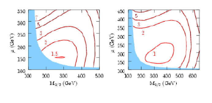
Figure 8: $\chi^{2}$ contours for $m_{16}=1.5$ TeV (Left) and $m_{16}=2$ TeV (Right). The shaded region is excluded by the chargino mass limit $m_{\tilde{\chi}^{+}}>103$ GeV.

Fig. 8 (Left) shows the constant $\chi^{2}$ contours for $m_{16}=1.5$ TeV in the case of Just So squark and slepton masses. We find acceptable fits ($\chi^{2}<3$) for $A_{0}\sim-1.9\;m_{16}$, $m_{10}\sim 1.4\;m_{16}$ and $m_{16}\geq 1.2$ TeV. The best fits are for $m_{16}\geq 2$ TeV with $\chi^{2}<1$. Fig. 1 (Right) shows the constant $\chi^{2}$ contours for $m_{16}=2$ TeV.

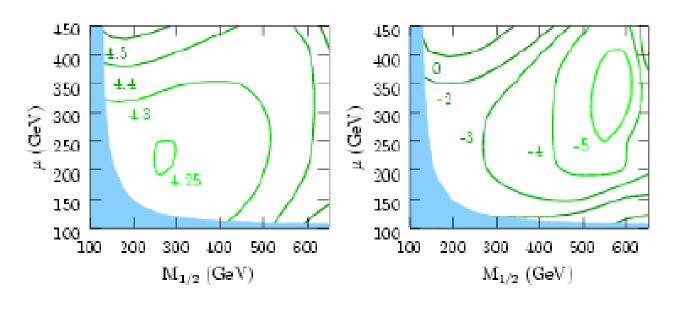
Figure 9: Contours of constant $m_{b}(m_{b})$[GeV] (Left) and $\Delta m_{b}\;$in % (Right) for $m_{16}=2$ TeV.

Fig. 9 gives the constant $m_{b}(m_{b})$ and $\delta m_{b}/m_{b}$ contours for $m_{16}=2$ TeV. We see that the best fits, near the central value, are found with $-4\%\leq\delta m_{b}/m_{b}\leq-2$%. The chargino contribution (Eqn. 93) is typically opposite in sign to the gluino (Eqn. 92), since $A_{t}$ runs to an infrared fixed point $\propto-M_{1/2}$ (see for example, [Carena et al(1994)]). Hence in order to cancel the positive contribution of both the log (Eqn. 94) and gluino contributions, a large negative chargino contribution is needed. This can be accomplished for $-A_{t}>m_{\tilde{g}}$ and $m_{\tilde{t}_{1}}\ll m_{\tilde{b}_{1}}$. The first condition can be satisfied for $A_{0}$ large and negative, which helps pull $A_{t}$ away from its infrared fixed point. The second condition is also aided by large $A_{t}$. However in order to obtain a large enough splitting between $m_{\tilde{t}_{1}}$ and $m_{\tilde{b}_{1}}$, large values of $m_{16}$ are needed. Note, that for Just So scalar masses, the lightest stop is typically lighter than the sbottom. We typically find $m_{\tilde{b}_{1}}\sim 3\;m_{\tilde{t}_{1}}$. On the other hand, D term splitting with $D_{X}>0$ gives $m_{\tilde{b}_{1}}\leq m_{\tilde{t}_{1}}$. As a result in the case of Just So boundary conditions excellent fits are obtained for top, bottom and tau masses; while for D term splitting the best fits give $m_{b}(m_{b})\geq 4.59$ GeV.

The bottom line is that Yukawa unification is only possible in a narrow region of SUSY parameter space with

$$A_{0}\sim-1.9\;m_{16},\;\;m_{10}\sim 1.4\;m_{16},\;\;\;$$ (95)

$$(\mu,\ M_{1/2})\sim 100-500\;{\rm GeV\;\;and}\;\;m_{16}\geq 1.2\;{\rm TeV}.$$ (96)

It would be nice to have some a priori reason for the fundamental SUSY breaking mechanism to give these soft SUSY breaking parameters. However, without such an a priori explanation, it is all the more interesting and encouraging to recognize two additional reasons for wanting to be in this narrow region of parameter space.

1. One mechanism for suppressing large flavor violating processes in SUSY theories is to demand heavy first and second generation squarks and sleptons (with mass $\gg$ TeV) and the third generation scalars lighter than a TeV. Since the third generation scalars couple most strongly to the Higgs, this limit can still leave a “naturally” light Higgs [Dimopoulos and Giudice (1995)]. It was shown that this inverted scalar mass hierarchy can be obtained “naturally,” i.e. purely as a consequence of renormalization group running from $M_{G}$ to $M_{Z}$, with suitably chosen soft SUSY breaking boundary conditions at $M_{G}$ [Bagger et al(1999,2000)]. All that is needed is $SO(10)$ boundary conditions for the Higgs mass (i.e. $m_{10}$), squark and slepton masses (i.e. $m_{16}$) and a universal scalar coupling $A_{0}$. In addition, they must be in the ratio [Bagger et al(2000)]

   $$A_{0}^{2}=2\ m_{10}^{2}=4\ m_{16}^{2},\;\;\;{\rm with}\;\;\;m_{16}\gg\;{\rm TeV}.$$ (97)

2. In order to suppress the rate for proton decay due to dimension 5 operators one must also demand [Dermíšek et al(2001)]

   $$(\mu,\;M_{1/2})\ll m_{16},\;\;\;{\rm with}\;\;\;m_{16}>\ {\rm few\;TeV}.$$ (98)

5.1.2 Consequences for Higgs and SUSY Searches

In Fig. 10 we show the constant light Higgs mass contours for $m_{16}=1.5$ and $2$ TeV (solid lines) with the constant $\chi^{2}$ contours overlayed (dotted lines). Yukawa unification for $\chi^{2}\leq 1$ clearly prefers a light Higgs with mass in a narrow range, 112 - 118 GeV.

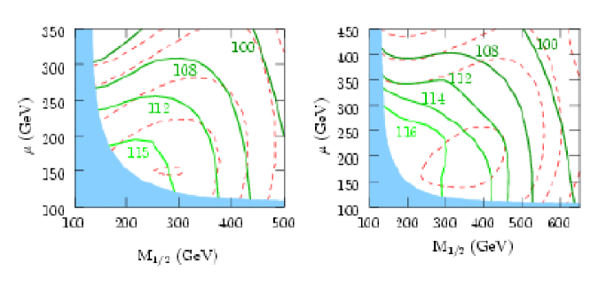
Figure 10: Contours of constant $m_{h}$ [GeV] (solid lines) with $\chi^{2}$ contours from Fig. 1 (dotted lines) for $m_{16}=1.5$ TeV (Left) and $m_{16}=2$ TeV (Right).

In this region the CP odd $A$, the heavy CP even Higgs $H$ and the charged Higgs bosons $H^{\pm}$ are also quite light. In addition we find the mass of $\tilde{t}_{1}\sim(150-250)$ GeV, $\tilde{b}_{1}\sim(450-650)$ GeV, $\tilde{\tau}_{1}\sim(200-500)$ GeV, $\tilde{g}\sim(600-1200)$ GeV, $\tilde{\chi}^{+}\sim(100-250)$ GeV, and $\tilde{\chi}^{0}\sim(80-170)$ GeV. All first and second generation squarks and sleptons have mass of order $m_{16}$. The light stop and chargino may be visible at the Tevatron. With this spectrum we expect $\tilde{t}_{1}\rightarrow\tilde{\chi}^{+}\;b$ with $\tilde{\chi}^{+}\rightarrow\tilde{\chi}^{0}_{1}\;\bar{l}\;\nu$ to be dominant. Lastly $\tilde{\chi}^{0}_{1}$ is the LSP and possibly a good dark matter candidate (see for example, [Roszkowski et al(2001)] and Fig. 11).

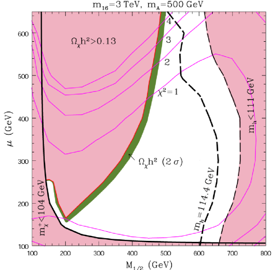
Figure 11: Constant $\chi^{2}$ contours as a function of $\mu,\ M_{1/2}$ for $m_{16}=3$ TeV. Note the much larger range of parameters with $\chi^{2}<1$ for this larger value of $m_{16}$. The green shaded region is consistent with the recent WMAP data for dark matter abundance of the neutralino LSP. The light shaded region in the lower left hand corner (separated by the solid line) is excluded by chargino mass limits, while the light shaded region in the upper left (right side) is excluded by a cosmological dark matter abundance which is too large (Higg mass which is too light). To the left of the vertical contour for a light Higgs with mass at the experimental lower limit, the light Higgs mass increases up to a maximum value of about 121 GeV at the lower left-hand acceptable boundary.

Our analysis thus far has only included third generation Yukawa couplings; hence no flavor mixing. If we now include the second family and 2-3 family mixing, consistent with $V_{cb}$, we obtain new and significant constraints on $m_{\tilde{t}_{1}}$ and $m_{A}$. The stop mass is constrained by $B(b\rightarrow s\gamma)$ to satisfy $m_{\tilde{t}}^{MIN}>450$ GeV (unfortunately increasing the bottom quark mass). In addition, as shown by [Choudhury and Gaur (1999), Babu and Kolda (2000), Dedes et al(2001), Isidori and Retico (2001)] the one loop SUSY corrections to CKM mixing angles (see Blažek et al(1995)) result in flavor violating neutral Higgs couplings. As a consequence the CDF bound on the process $B_{s}\rightarrow\mu^{+}\mu^{-}$ places a lower bound on $m_{A}\geq 200$ GeV [Choudhury and Gaur (1999), Babu and Kolda (2000), Dedes et al(2001), Isidori and Retico (2001)]. $\chi^{2}$, on the other hand, increases as $m_{A^{0}}$ increases. However the increase in $\chi^{2}$ is less than 60% for $m_{A}<400$ GeV. Note, the $H^{\pm},\ H^{0}$ masses increase linearly with $m_{A}$.

5.1.3 SU(5) Yukawa unification

Now consider Yukawa unification in SU(5). In this case we only have the GUT relation $\lambda_{b}=\lambda_{\tau}$. The RG running of the ratio $\lambda_{b}/\lambda_{\tau}$ to low energies then increases (decreases) due to QCD (Yukawa) interactions. In addition, neglecting Yukawa interactions, this ratio is too large at the weak scale. For a top quark mass $M_{t}\sim 175$ GeV, a good fit is obtained for small $\tan\beta\sim 1$ [Dimopoulos et al(1992), Barger et al(1993)]. In this case, only the top quark Yukawa coupling is important. While for large $\tan\beta\sim 50$ we recover the results of SO(10) Yukawa unification. For a recent analysis, see [Barr and Dorsner (2003)].

5.2 Fermion mass hierarchy & Family symmetry

In both the standard model and the MSSM, the observed pattern of fermion masses and mixing angles has its origin in the Higgs-quark and Higgs-lepton Yukawa couplings. In the standard model these complex $3\times 3$ matrices are arbitrary parameters which are under constrained by the 13 experimental observables (9 charged fermion masses and 4 quark mixing angles). [We consider neutrino masses and mixing angles in the following section.] In the MSSM more of the Yukawa parameters are in principle observable, since left and right-handed fermion mixing angles affect squark and slepton masses and mixing. [We consider this further in Section 5.4.] What can SUSY say about fermion masses? SUSY alone constrains the Yukawa sector of the theory simply by requiring that all terms in the superpotential are holomorphic. Combined with flavor symmetries, the structure of fermion masses can be severely constrained. On the other hand, the only information we have about these flavor symmetries is the fermion masses and mixing angles themselves, as well as the multitude of constraints on flavor violating interactions. There are, perhaps, many different theories with different family symmetries that fit the precision low energy data (including fermion masses and mixing angles). The goal is to find a set of predictive theories, i.e with fewer arbitrary parameters than data, that fit this data. The more predictive the theory, the more testable it will be. Within the context of the MSSM, theories have been constructed with U(1) family symmetries [Binetruy et al(1996), Elwood et al(1997,1998), Irges et al(1998), Faraggi and Pati (1998), Kakizaki and Yamaguchi (2002), Dreiner et al(2003)], with discrete family symmetries [Frampton and Kephart (1995a,b), Hall and Murayama (1995), Carone et al(1996), Carone and Lebed (1999), Frampton and Rasin (2000), Aranda et al(2000)] or non-abelian family symmetries [Hall and Randall (1990), Dine et al(1993), Nir and Seiberg (1993), Pouliot and Seiberg (1993), Leurer et al(1993,1994), Pomarol and Tommasini (1995), Hall and Murayama (1995), Dudas et al(1995,1996), Barbieri et al(1996), Arkani-Hamed et al(1995,1996), Barbieri et al(1997), Eyal (1998)]. However, the most predictive theories combine both grand unified and family symmetries [Kaplan and Schmaltz (1994), Babu and Mohapatra (1995), Lucas and Raby (1996), Frampton and Kong (1996), Blažek et al(1997), Barbieri and Hall (1997), Barbieri et al(1997), Allanach et al(1997), Berezhiani (1998), Blažek et al(1999,2000), Dermíšek and Raby (2000), Shafi and Tavartkiladze (2000), Albright and Barr (2000,2001), Altarelli et al(2000), Babu et al(2000), Berezhiani and Rossi (2001), Kitano and Mimura (2001), Maekawa (2001), King and Ross (2003), Chen and Mahanthappa (2003), Raby (2003), Ross and Velasco-Sevilla (2003), Goh et al(2003), Aulakh et al(2003)]. The Yukawa couplings in a predictive theory are completely defined in terms of the states and symmetries of the theory. The ultimate goal of this program is to construct one (or more) of these predictive theories, providing good fits to the data, in terms of a more fundamental theory, such as M theory. Only then will higher order corrections to the theory be under full control. It is important to remark at this stage that any theory, derived from some fundamental theory, includes non-renormalizable higher dimension operators. The higher dimension operators are suppressed by the fundamental scale (for example, the string scale $M_{S}$) which is assumed to be greater than the GUT scale $M_{G}$. As we shall now see, these higher dimension operators are useful in explaining the hierarchy of fermion masses.

The $3\times 3$ up, down and charged lepton mass matrices are given by the mass terms:

$${\cal L}_{mass}=u\ Y_{u}\ \bar{u}\ \langle H_{u}\rangle\ + \;\;\;d\ Y_{d}\ \bar{d}\ \langle H_{d}\rangle\ + \;\;\;e\ Y_{e}\ \bar{e}\ \langle H_{d}\rangle.$$ (99)

Empirical descriptions of the quark mass matrices have been discussed in all the papers referenced above. As an example, consider the following theory incorporating the hierarchy of masses and mixing angles in an SU(5) SUSY GUT with U(1) family symmetry by [Altarelli et al(2000)]

$$Y_{u}=\left(\begin{array}[]{ccc}\lambda^{6}&\lambda^{5}&\lambda^{3}\\ \lambda^{5}&\lambda^{4}&\lambda^{2}\\ \lambda^{3}&\lambda^{2}&1\end{array}\right), \;\;\;\;Y_{d}=Y_{e}^{T}=\left(\begin{array}[]{ccc}\lambda^{5}&\lambda^{3}&\lambda^{3}\\ \lambda^{4}&\lambda^{2}&\lambda^{2}\\ \lambda^{2}&1&1\end{array}\right)\lambda^{4}.$$ (106)

Order 1 coefficients of the matrix elements are implicit. We then obtain the rough empirical relations.

$$m_{c}/m_{t}\ \sim\ m_{u}/m_{c} \;\sim\ V_{cb}^{2} \ \approx\ \lambda^{4}$$ (107)

$$m_{s}/m_{b}\ \sim\ m_{d}/m_{s} \;\sim\ V_{us}^{2} \ \approx\ \lambda^{2}.$$

In addition, the Yukawa matrices for down quarks and charged leptons satisfy the SU(5) relations

$$\lambda_{b}=\lambda_{\tau}, \;\;\lambda_{s}=\lambda_{\mu}, \;\;\lambda_{d}=\lambda_{e}.$$ (108)

This works for the third generation, as discussed in Section 5.1.3, however it clearly doesn’t work for the first and second generations, where it gives the unacceptable prediction

$$20\;\approx\;m_{s}/m_{d}\;=\;m_{\mu}/m_{e}\;\approx\;200.$$ (109)

Hence in this SU(5) model with U(1) family symmetry, an additional Higgs in the 75 dimensional representation (with U(1) charge zero) also contributes to down quark and charged lepton Yukawa matrices [Altarelli et al(2000)]. The arbitrary, order one coefficients for each term in the Yukawa matrix are then fit to the quark masses and mixing angles and charged lepton masses. Note in this theory there are more arbitrary parameters, than fermion mass observables; hence there are no predictions for fermion masses and mixing angles. Nevertheless, predictions for proton decay are now obtained. Moreover, given a model for soft SUSY breaking terms like the CMSSM, one can also predict rates for flavor violating processes.

The structure for these Yukawa matrices are determined by the U(1) family symmetry, spontaneously broken by a scalar field $\phi$ with U(1) charge $-1$. The symmetry breaking field $\phi$ is inserted into each element of the Yukawa matrix in order to obtain a U(1) invariant interaction. This results in effective higher dimensional operators suppressed by a scale $M$ with $\lambda\sim\langle\phi\rangle/M$. This is the Froggatt-Nielsen mechanism [Froggatt and Nielsen (1979), Berezhiani (1983,1985), Dimopoulos (1983), Bagger et al(1984)]. For a review see [Raby (1995)]. Given the U(1) charge assignments in Table 5 [Altarelli et al(2000)] we obtain the Yukawa matrices in Eqn. 106.

Table 5: U(1) charge $Q$ of Higgs and matter fields in the (1st,2nd,3rd) generation.

• field	$H_{u}$	$H_{d}$	10 = {$Q$,  $\bar{u}$,  $\bar{e}$}	$\bar{5}$ = {$\bar{d}$,  L}	$\bar{\nu}$
  $Q$	-2	1	(4,3,1)	(4,2,2)	(1,-1,0)

Similar mass matrices using analogous U(1) family symmetry arguments have also been considered.

Using a non-abelian family symmetry, such as SU(2) $\times$ U(1) or SU(3) or discrete subgroups of SU(2), models with fewer arbitrary parameters in the Yukawa sector have been constructed. An example of a very predictive SO(10) SUSY GUT with SU(2) $\times$ U(1)ⁿ family symmetry is given by [Barbieri et al(1997(a,b),1999), Blažek et al(1999,2000)]. An analogous model can be obtained by replacing the SU(2) family symmetry with a discrete subgroup D(3) [Dermíšek and Raby (2000)]. The model incorporates the Froggatt-Nielsen mechanism with a hierarchy of symmetry breaking VEVs explaining the hierarchy of fermion masses. The effective fermion mass operators are given in Fig. 12. In particular, the family symmetry breaking pattern

$$SU_{2}\times U_{1}\;\;\;\longrightarrow\;\;\;U_{1}\;\;\;\longrightarrow\;\;\;{\rm nothing}$$ (110)

with small parameters $\epsilon\approx\tilde{\epsilon}$ and $\epsilon^{\prime}$, respectively, gives the hierarchy of masses with the 3rd family $\gg$ 2nd family $\gg$ 1st family. It includes the Georgi - Jarlskog [Georgi and Jarlskog (1979)] solution to the unacceptable SU(5) relation (Eqn. 109) with the improved relation

$$m_{s}\;\sim\;\frac{1}{3}m_{\mu},\;\; m_{d}\;\sim\;3m_{e}.$$ (111)

This is obtained naturally using the VEV

$$\langle 45\rangle=(B-L)\ M_{G}.$$ (112)

In addition, it gives the SO(10) relation for the third generation

$$\lambda_{t}=\lambda_{b}=\lambda_{\tau}=\lambda_{\nu_{\tau}}=\lambda$$ (113)

and it uses symmetry arguments to explain why $m_{u}<m_{d}$ even though $m_{t}\gg m_{b}$. Finally the $SU_{2}$ family symmetry suppresses flavor violation such as $\mu\rightarrow e\gamma$. When SO(10) $\times$ SU(2) $\times$ U(1)ⁿ is broken to the MSSM the effective Yukawa couplings (Eqn. 122) are obtained. The superpotential for this simple model is given by

$$W\supset 16_{3}\ 10\ 16_{3}+16_{a}\ 10\ \chi^{a}$$

$$+\bar{\chi}_{a}\ (M_{\chi}\ \chi^{a}+\ 45\ \frac{\phi^{a}}{\hat{M}}\ 16_{3}\ +\ 45\ \frac{S^{ab}}{\hat{M}}\ 16_{b}+A^{ab}\ 16_{b})$$

where $\phi^{a},\;S^{ab}=S^{ba},\;A^{ab}=-A^{ba}$ are the familon fields whose VEVs break the family symmetry, $M_{\chi}=\hat{M}\ (1+\alpha\ X+\beta\ Y)$ with $X,\ Y$ charges associated with U(1)${}_{X,\ Y}$, the orthogonal U(1) subgroups of SO(10), and { $\chi^{a},\bar{\chi}_{a}$ } are the heavy Froggatt-Nielsen fields. After the heavy $\chi$ states are integrated out of the theory we obtain the effective fermion mass operators given in Fig. 12.

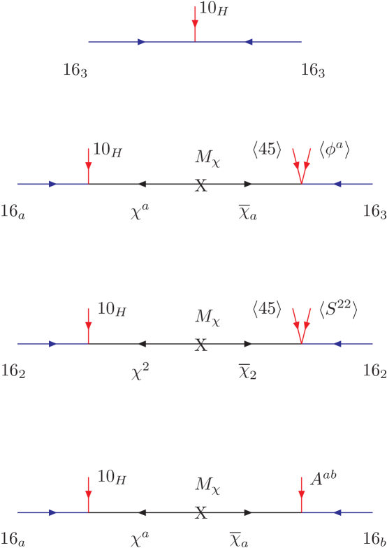
Figure 12: Effective fermion mass operators. The fields $\phi^{a},\ S^{ab}=S^{ba},A^{ab}=-A^{ba}$ spontaneously break the SU(2) $\times$ U(1)ⁿ family symmetry with $\epsilon\propto\langle\phi^{2}\rangle$, $\tilde{\epsilon}\propto\langle S^{22}\rangle$, and $\epsilon^{\prime}\propto\langle A^{12}\rangle$.

These four Feynman diagrams lead to the following Yukawa matrices for quarks and charged leptons.

$$Y_{u}= \left(\begin{array}[]{ccc}0&\epsilon^{\prime}\ \rho&-\epsilon\ \xi\\ -\epsilon^{\prime}\ \rho&\tilde{\epsilon}\ \rho&-\epsilon\\ \epsilon\ \xi&\epsilon&1\end{array}\right)\;\lambda$$ (118)

$$Y_{d}= \left(\begin{array}[]{ccc}0&\epsilon^{\prime}&-\epsilon\ \sigma\ \xi\\ -\epsilon^{\prime}&\tilde{\epsilon}&-\epsilon\ \sigma\\ \epsilon\ \xi&\epsilon&1\end{array}\right)\;\lambda$$ (122)

$$Y_{e}= \left(\begin{array}[]{ccc}0&-\epsilon^{\prime}&3\ \epsilon\ \xi\\ \epsilon^{\prime}&3\ \tilde{\epsilon}&3\ \epsilon\\ -3\ \epsilon\ \xi&-3\ \epsilon&1\end{array}\right)\;\lambda$$ (126)

with

$$\xi\;\;=\;\;\langle\phi^{1}\rangle/\langle\phi^{2}\rangle; \;\;\tilde{\epsilon}\;\;\propto\;\;\langle S^{22}\rangle/\hat{M};$$ (127)

$$\epsilon\;\;\propto\;\;\langle\phi^{2}\rangle/\hat{M}; \;\;\epsilon^{\prime}\;\;\sim\;\;\langle A^{12}\rangle/\hat{M};$$

$$\sigma\;\;=\;\;\frac{1+\alpha}{1-3\alpha}; \;\;\rho\;\;\sim\;\;\beta\,\ll\,\alpha.$$

The model has only 9 arbitrary Yukawa parameters (6 real parameters {$|\lambda|,\ |\epsilon|,\ |\tilde{\epsilon}|,\ |\rho|,\ |\sigma|,\ |\epsilon^{\prime}|$} and three phases {$\Phi_{\epsilon}=\Phi_{\tilde{\epsilon}},\ \Phi_{\rho},\ \Phi_{\sigma}$}) to fit the 13 fermion masses and mixing angles (we have taken $\xi=0$). The fit to the low energy data is given in Table 6. More details of this fit are found in [Blažek et al(1999)] and the predictions for proton decay are found in [Dermíšek et al(2001)]. Note, the model fits most of the precision electroweak data quite well.

Table 6: Fit to fermion masses and mixing angles for SO(10) GUT with SU(2) $\times$ U(1)ⁿ family symmetry [Blažek et al(1999)].

• Observable	Data($\sigma$)masses in GeV	Theory
  $M_{Z}$	91.187  (0.091)	91.17
  $M_{W}$	80.388  (0.080)	80.40
  $G_{\mu}\cdot 10^{5}$	1.1664  (0.0012)	1.166
  $\alpha_{EM}^{-1}$	137.04  (0.14)	137.0
  $\alpha_{s}(M_{Z})$	0.1190  (0.003)	0.1174
  $\rho_{new}\cdot 10^{3}$	-1.20  (1.3)	+0.320
  $M_{t}$	173.8  (5.0)	175.0
  $m_{b}(M_{b})$	4.260  (0.11)	4.328
  $M_{b}-M_{c}$	3.400  (0.2)	3.421
  $m_{s}$	0.180  (0.050)	0.148
  $m_{d}/m_{s}$	0.050  (0.015)	0.0589
  $Q^{-2}$	0.00203  (0.00020)	0.00201
  $M_{\tau}$	1.777  (0.0018)	1.776
  $M_{\mu}$	0.10566  (0.00011)	.1057
  $M_{e}\cdot 10^{3}$	0.5110  (0.00051)	0.5110
  $V_{us}$	0.2205  (0.0026)	0.2205
  $V_{cb}$	0.03920  (0.0030)	0.0403
  $V_{ub}/V_{cb}$	0.0800  (0.02)	0.0691
  $\hat{B}_{K}$	0.860  (0.08)	0.8703
  $B(b\rightarrow\ s\gamma)\ \cdot 10^{4}$	3.000  (0.47)	2.995
  TOTAL $\chi^{2}$	3.39

In [Blažek et al(1999)] there is also a prediction for $\sin 2\beta=0.54$ which should be compared to the present experimental value $0.727\ (0.036)$. The prediction for $\sin 2\beta$ is off by 5 $\sigma$. In addition the present experimental value for $V_{ub}/V_{cb}$ is $0.086\ (0.008)$, hence this fit (Table 6) is somewhat worse than before. Both of these quantities are predictions due solely to the zeros in the 11, 13 and 31 elements of the Yukawa matrices [Hall and Rasin (1993), Roberts et al(2001), Kim et al(2004)]. These poor fits are remedied with the addition of a non-vanishing 13 / 31 element, i.e. $\xi\neq 0$. In this case a good fit is obtained with one additional real parameter [Kim et al(2004)].

Table 7: Input parameters at $M_{G}$ for fit in Table 6 [Blažek et al(1999)].

• (1/$\alpha_{G},\,M_{G},\,\epsilon_{3}$) =	($24.52,\,3.05\cdot 10^{16}$ GeV,$\,-4.08$%),
  ($\lambda,\,\epsilon,\,\sigma,\,\tilde{\epsilon},\,\rho,\,\epsilon^{\prime},\,\xi$ ) =	($0.79,\,0.045,\,0.84,\,0.011,\,0.043,\,0.0031,\,0.00$),
  ($\Phi_{\sigma},\,\Phi_{\epsilon}=\Phi_{\tilde{\epsilon}},\,\Phi_{\rho}$) =	($0.73,\,-1.21,\,3.72$)rad,
  ($m_{16},\,M_{1/2},\,A_{0},\,\mu(M_{Z})$) =	($1000,\,300,\,-1437,\,110$) GeV,
  ($(m_{H_{d}}/m_{16})^{2},\,(m_{H_{u}}/m_{16})^{2},\,$tan$\beta$) =	($2.22,\,1.65,\,53.7$)

5.3 Neutrino masses

The combined data from all neutrino experiments can be fit by the hypothesis of neutrino oscillations with the neutrino masses and mixing angles given by

$$\Delta m^{2}_{atm}= |m_{3}^{2}-m_{2}^{2}|\approx 3\times 10^{-3}\;{\rm eV}^{2}$$

$$\sin 2\theta_{atm}\approx 1$$

$$\Delta m^{2}_{sol}= |m_{2}^{2}-m_{1}^{2}|\approx 7\times 10^{-5}\;{\rm eV}^{2}$$

$$0.8<\sin 2\theta_{sol}<1$$

For recent theoretical analyses of the data, see [Barger et al(2003), Maltoni et al(2003), Gonzales-Garcia and Peña-Garay (2003)]. This so-called bi-large neutrino mixing is well described by the PMNS mixing matrix

$$\left(\begin{array}[]{c}\nu_{e}\\ \nu_{\mu}\\ \nu_{\tau}\end{array}\right)\approx \left(\begin{array}[]{ccc}c_{sol}&s_{sol}&0\\ -s_{sol}/\sqrt{2}&c_{sol}/\sqrt{2}&1/\sqrt{2}\\ -s_{sol}/\sqrt{2}&c_{sol}/\sqrt{2}&-1/\sqrt{2}\end{array}\right)\;\left(\begin{array}[]{c}\nu_{1}\\ \nu_{2}\\ \nu_{3}\end{array}\right).$$ (138)

which takes mass eigenstates into flavor eigenstates. The 1-3 mixing angle satisfies $\sin\theta_{13}<0.2$ at 3 $\sigma$ [Maltoni et al(2003)].

Using the See-Saw mechanism [Yanagida (1979), Glashow (1979), Gell-Mann et al(1979), Mohapatra and Senjanovic (1980)], neutrino masses are given in terms of two completely independent $3\times 3$ mass matrices, i.e. the Dirac mass matrix $m_{\nu}$ and a Majorana mass matrix $M_{N}$ via the formula ${\cal M}_{\nu}=m_{\nu}^{T}\ M_{N}^{-1}\ m_{\nu}$. The smallness of neutrino masses is explained by the large Majorana mass scale, of order $10^{14}-10^{15}$ GeV; very close to the GUT scale. In addition, the large mixing angles needed to diagonalize ${\cal M}_{\nu}$ can be directly related to large mixing in $m_{\nu}$, in $M_{N}$ or in some combination of both. Lastly, the Dirac neutrino mass matrix $m_{\nu}$ is constrained by charged fermion masses in SO(10), but not in SU(5) where it is completely independent.

The major challenge for theories of neutrino masses is to obtain two large mixing angles; as compared to charged fermions where we only have small mixing angles in $V_{CKM}$. There are several interesting suggestions for obtaining large mixing angles in the literature. [For recent reviews of models of neutrino masses, see [Altarelli and Feruglio (2003), Altarelli et al(2003), King (2003)].]

• Degenerate neutrinos and RG running [Mohapatra et al(2003), Casas et al(2003)],

  It was shown that starting with three degenerate Majorana neutrinos and small mixing angles at a GUT scale, that RG running can lead to bi-large neutrino mixing at low energies.

• Minimal renormalizable SO(10) [Goh et al(2003), Bajc et al(2003)],

  SO(10) with Higgs in the 10 and $\overline{126}$ representations can give predictable theories of fermion masses with naturally large neutrino mixing angles.

• Dominant Majorana neutrinos [King (1998,2000)],

  It was shown that large neutrino mixing can be obtained via coupling to a single dominant right handed neutrino.

• Minimal Majorana sector [Frampton et al(2002), Raidal and Strumia (2003), Raby (2003)],

  It was shown that a simple model with two right handed neutrinos can accommodate bi-large neutrino mixing with only one CP violating phase. In such a theory, CP violating neutrino oscillations measured in low energy accelerator experiments are correlated with the matter – anti-matter asymmetry obtained via leptogenesis.

• Lopsided charged lepton and down quark matrices [Lola and Ross (1999), Nomura and Yanagida (1999), Albright and Barr (2000(a,b),2001), Altarelli et al(2000), Barr and Dorsner (2003)].

  In SU(5) (or even in some SO(10) models) the down quark mass matrix is related to the transpose of the charged lepton mass matrix. A large left-handed $\mu-\tau$ mixing angle is thus directly related to a large right-handed $s-b$ mixing angle. Whereas right-handed quark mixing angles are not relevant for CKM mixing, the large left-handed charged lepton mixing angle can give large $\nu_{\mu}-\nu_{\tau}$ mixing.

Let us now consider the last two mechanisms in more detail.

5.3.1 SU(5) $\times$ U(1) flavor symmetry

One popular possibility has the large $\nu_{\mu}-\nu_{\tau}$ mixing in the Dirac charged Yukawa matrix with

$$Y_{e}=\left(\begin{array}[]{ccc}\lambda^{5}&\lambda^{4}&\lambda^{2}\\ \lambda^{3}&\lambda^{2}&1\\ \lambda^{3}&\lambda^{2}&1\end{array}\right)\lambda^{4} =Y_{d}^{T}.$$ (142)

The neutrino Dirac Yukawa matrix and the Majorana matrix are given by

$$Y_{\nu}=\left(\begin{array}[]{ccc}\lambda^{3}&\lambda&\lambda^{2}\\ \lambda&0&1\\ \lambda&0&1\end{array}\right)$$ (146)

$$M_{N}=\left(\begin{array}[]{ccc}\lambda^{2}&1&\lambda\\ 1&0&0\\ \lambda&0&1\end{array}\right)$$ (150)

where we use the results of [Altarelli et al(2000)]. The light neutrino mass matrix is given by the standard See-Saw formula. We obtain:

$${\cal M}_{\nu}=U_{e}^{tr}\ \left(\begin{array}[]{ccc}\lambda^{4}&\lambda^{2}&\lambda^{2}\\ \lambda^{2}&1&1\\ \lambda^{2}&1&1\end{array}\right)\ U_{e}\ v_{u}^{2}/M.$$ (154)

where $v_{u}$ is the VEV of the Higgs doublet giving mass to the up quarks, $M$ is the heavy Majorana mass scale and all entries in each matrix are specified up to order one coefficients. $U_{e}$ is the mixing matrix taking left-handed charged leptons into the mass eigenstate basis. It is given by

$$\left(\begin{array}[]{ccc}m_{e}^{2}&0&0\\ 0&m_{\mu}^{2}&0\\ 0&0&m_{\tau}^{2}\end{array}\right)= U_{e}^{tr}\ (Y_{e}\ Y_{e}^{\dagger})\ U_{e}^{*}\ \langle H_{d}\rangle^{2}$$ (158)

where

$$Y_{e}\ Y_{e}^{\dagger}=\left(\begin{array}[]{ccc}\lambda^{4}&\lambda^{2}&\lambda^{2}\\ \lambda^{2}&1&1\\ \lambda^{2}&1&1\end{array}\right)$$ (162)

up to order one coefficients. It is clear that without order one coefficients, the neutrino mixing matrix is the identity matrix. Hence the arbitrary order one coefficients are absolutely necessary to obtain bi-large neutrino mixing. Hierarchical neutrino masses with $m_{3}\gg m_{2}\gg m_{1}$ and bi-large neutrino mixing can naturally be obtained [Altarelli and Feruglio (2003)].

Of course, different U(1) charge assignments for all the fields can lead to other experimentally acceptable solutions to the solar neutrino problem. For a review and further references, see [Altarelli and Feruglio (2003)].

5.3.2 $SO_{10}\times[SU_{2}\times U_{1}^{n}]_{FS}$ model

Within the context of the $SO_{10}\times[SU_{2}\times U_{1}^{n}]_{FS}$ model, bi-large neutrino mixing is naturally obtained using the mechanism of the minimal two Majorana neutrino sector. The Dirac neutrino mass is fixed once charged fermion masses and mixing angles are fit. It is given by the formula:

$$Y_{\nu}= \left(\begin{array}[]{ccc}0&-\epsilon^{\prime}\ \omega&{3\over 2}\ \epsilon\ \xi\ \omega\\ \epsilon^{\prime}\ \omega&3\ \tilde{\epsilon}\ \omega&{3\over 2}\ \epsilon\ \omega\\ -3\ \epsilon\ \xi\ \sigma&-3\ \epsilon\ \sigma&1\end{array}\right)\;\lambda$$ (166)

with $\omega\;\;=\;\;2\,\sigma/(2\,\sigma-1)$ and the Dirac neutrino mass matrix given by $m_{\nu}\equiv Y_{\nu}\frac{v}{\sqrt{2}}\sin\beta$. Of course, all the freedom is in the Majorana neutrino sector. The FGY ansatz [Frampton et al(2002)] is obtained with the following Majorana neutrino sector [Raby (2003)]:

$$W_{neutrino}= \frac{\overline{16}}{\hat{M}}\left(N_{1}\ \tilde{\phi}^{a}\ 16_{a}\ +\ N_{2}\ \phi^{a}\ 16_{a}\ +\ N_{3}\ \theta\ 16_{3}\right)$$

$$+\frac{1}{2}\left(S_{1}\ N_{1}^{2}\ +\ S_{2}\ N_{2}^{2}\right)$$

where {$N_{i},\;i=1,2,3$} are SO(10) and SU(2) - flavor singlets. In this version of the theory, the symmetric two index tensor flavon field $S^{ab}$ is replaced by an SU(2) doublet $\tilde{\phi}^{a}$ such that $S^{ab}\equiv\tilde{\phi}^{a}\ \tilde{\phi}^{b}/\hat{M}$. Note, since the singlet $N_{3}$ has no large Majorana mass, it gets a large Dirac mass by mixing directly with $\bar{\nu}_{3}$ at the GUT scale. Thus $\bar{\nu}_{3}$ is removed from the See-Saw mechanism and we effectively have only two right-handed neutrinos taking part.

Integrating out the heavy neutrinos we obtain the light neutrino mass matrix given by

$${\cal M}_{\nu}= U_{e}^{tr}\;[\ D^{tr}\ \hat{M}_{N}^{-1}\ D\ ]\;U_{e}$$ (167)

where $U_{e}$ is the unitary matrix diagonalizing the charge lepton mass matrix and

$$D^{tr}\equiv\left(\begin{array}[]{cc}a&0\\ a^{\prime}&b\\ 0&b^{\prime}\end{array}\right),\;\;\;\;\; \hat{M}_{N}\equiv\left(\begin{array}[]{cc}\langle S_{1}\rangle&0\\ 0&\langle S_{2}\rangle\end{array}\right)$$ (173)

with

$$b\equiv \epsilon^{\prime}\ \omega\ \lambda\ (M_{2}/\langle\phi^{1}\rangle)\ \frac{\hat{M}}{v_{16}}\frac{v\sin\beta}{\sqrt{2}}$$ (174)

$$b^{\prime}\equiv -3\ \epsilon\ \xi\ \sigma\ \lambda\ (M_{2}/\langle\phi^{1}\rangle)\ \frac{\hat{M}}{v_{16}}\frac{v\sin\beta}{\sqrt{2}}.$$

$$a\equiv -\epsilon^{\prime}\ \omega\ \lambda\ (M_{1}/\langle\tilde{\phi}^{2}\rangle)\ \frac{\hat{M}}{v_{16}}\frac{v\sin\beta}{\sqrt{2}}$$

$$a^{\prime}\equiv (-\epsilon^{\prime}\ \xi^{-1}+3\ \tilde{\epsilon})\ \omega\ \lambda\ (M_{1}/\langle\tilde{\phi}^{2}\rangle)\ \frac{\hat{M}}{v_{16}}\frac{v\sin\beta}{\sqrt{2}}.$$

We obtain

$$b\sim b^{\prime}$$ (175)

naturally, since $\epsilon^{\prime}\ \sim\ \epsilon\ \xi$. In addition we can accommodate

$$a\sim a^{\prime}$$ (176)

with minor fine-tuning O(1/10) since $\epsilon^{\prime}\ \xi^{-1}\ \sim\ \tilde{\epsilon}.$ Note, this is the Frampton-Glashow-Yanagida ansatz [Frampton et al(2002)] with a bi-large neutrino mixing matrix obtained naturally in a SUSY GUT.

5.4 Flavor Violation

Quarks and leptons come in different flavors: up, down, charm, strange, top, bottom; electron, muon, tau. We observe processes where bottom quarks can decay into charm quarks or up quarks. Hence quark flavors (for quarks with the same electric charge) are interchangeable. In the standard model, this is parametrized by the CKM mixing matrix. We now have direct evidence from neutrino oscillation experiments showing that tau, muon and electron numbers are not separately conserved. Yet, we have never observed muons changing into electrons. In supersymmetric theories there are many more possible ways in which both lepton and quark flavors can change. This is because scalar quarks and leptons carry the flavor quantum numbers of their SUSY partners. Thus flavor violation in the scalar sector can lead to flavor violation in the observed fermionic sector of the theory. This gives rise to the SUSY flavor problem. We consider two examples here: $\mu\rightarrow e\gamma$ or $B_{s}\rightarrow\mu^{+}\mu^{-}$. We show why SUSY GUTs and/or neutrino masses can cause enhanced flavor violation beyond that of the standard model. In this section we consider several ways to solve the SUSY flavor problem.

Figure 13: The one loop contribution to the process $\mu\rightarrow e\gamma$ proportional to an off-diagonal scalar muon - electron mass term in the charged lepton mass eigenstate basis.

But first let us illustrate the problem with a few of the dominant examples [Gabbiani et al(1996)]. In the first column of Table 8 we present four flavor violating observables with their experimental bounds. In the second and third columns we present the bounds on flavor violating scalar mass corrections

$$\delta_{ij}^{f}\equiv\Delta{m^{2}_{ij}}^{f}/\bar{m}^{2}$$ (177)

where $i,j=1,2,3$ are family indices, $\Delta{m^{2}_{ij}}^{f}$ is an off-diagonal scalar mass insertion for $f=$ {quark, lepton} flavor (treated to lowest non-trivial order in perturbation theory) in the flavor diagonal basis for quarks and leptons. $\bar{m}$ is the average squark or slepton mass squared. The subscripts $LL$ refer to left-handed squark or slepton mass insertions. There are separate limits on $RR$ and $LR$ mass insertions [Gabbiani et al(1996)] which are not presented here. The only difference between the second and third columns is the fiducial value of $\bar{m}^{2}$. Clearly as the mean squark or slepton mass increases, the fine tuning necessary to avoid significant flavor violation is dramatically reduced. As seen in Fig. 13, the amplitude for $\mu\rightarrow e\gamma$ is proportional to $\delta_{12}^{e}$ and is suppressed by $1/\bar{m}^{2}$, since it is an effective dimension 5 operator.

Table 8: Some constraints from the non-observation of flavor violation on squark, slepton and gaugino masses [Gabbiani et al(1996)]. For the electron electric dipole moment we use the relation $d_{N}^{e}\sim 2(100/m_{\tilde{l}}({\rm GeV}))^{2}sin\Phi_{A,B}\times 10^{-23}{\rm e\ cm}$.

• Observable	Experimental bound (1)	Experimental bound (2)
  $B(\mu\rightarrow e\gamma)<1.2\times 10^{-11}$	$|(\delta_{12}^{l})_{LL}|<2.1\times 10^{-3}(m_{\tilde{l}}({\rm GeV})/100)^{2}$	$|(\delta_{12}^{l})_{LL}|<0.8\ (m_{\tilde{l}}({\rm TeV})/2)^{2}$
  $\Delta m_{K}<3.5\times 10^{-12}$ MeV	$\sqrt{|Re(\delta_{12}^{d})^{2}_{LL}|}<1.9\times 10^{-2}(m_{\tilde{q}}({\rm GeV})/500)$	$\sqrt{|Re(\delta_{12}^{d})^{2}_{LL}|}<7.6\times 10^{-2}\ (m_{\tilde{q}}({\rm TeV})/2)$
  $\epsilon_{K}<2.28\times 10^{-3}$	$\sqrt{|Im(\delta_{12}^{d})^{2}_{LL}|}<1.5\times 10^{-3}(m_{\tilde{q}}({\rm GeV})/500)$	$\sqrt{|Re(\delta_{12}^{d})^{2}_{LL}|}<6.0\times 10^{-3}\ (m_{\tilde{q}}({\rm TeV})/2)$
  $d_{N}^{e}<4.3\times 10^{-27}{\rm e\ cm}$	$sin\Phi_{A,B}<4\times 10^{-4}\times(m_{\tilde{l}}({\rm GeV})/100)^{2}$	$sin\Phi_{A,B}<0.16\times(m_{\tilde{l}}\ ({\rm TeV})/2)^{2}$

5.4.1 The Origin of flavor violation in SUSY theories

There are three possible ways to avoid large flavor violation.

1. Having squarks and sleptons, with the same standard model gauge charges, be degenerate and, in addition, the cubic scalar interactions proportional to the Yukawa matrices.

2. Alignment of squark and slepton masses with quark and lepton masses.

   The fermion and scalar mass matrices are “aligned” when, in the basis where fermion masses are diagonal, the scalar mass matrices and cubic scalar interactions are approximately diagonal as well.

3. Heavy first and second generation squarks and sleptons.

The CMSSM (or mSUGRA) is an example of the first case. It has a universal scalar mass $m_{0}$ and tri-linear scalar interactions proportional to Yukawa matrices. These initial conditions correspond to a symmetry limit [Hall et al(1986)] – dubbed minimal flavor violation [Ciuchini et al(1998)]– where the only flavor violation occurs in the CKM matrix at the messenger scale for SUSY breaking, or in this case, the Planck scale. Gauge-mediated SUSY breaking, where squarks and sleptons obtain soft SUSY breaking masses via standard model gauge interactions, is another example of the first case (for a review, see [Giudice and Rattazzi (1999)]. In this case the messenger mass is arbitrary. Finally, within the context of perturbative heterotic string theory, dilaton SUSY breaking gives universal scalar masses at the string scale. For moduli SUSY breaking, on the other hand, scalar masses depend on modular weights, whose values are very model dependent.

Abelian flavor symmetries can be used to align quark (lepton) and the corresponding squark (slepton) mass matrices, but they still require one of the above mechanisms for obtaining degenerate scalar masses at zeroth order in symmetry breaking. Non-abelian symmetries, on the other hand, can both align fermion and scalar mass matrices and guarantee the degeneracy of the scalar masses at zeroth order.

Finally, since the most stringent limits from flavor violating processes come from the lightest two families, if the associated squarks and sleptons are heavy these processes are suppressed [Dimopoulos and Giudice (1995)]. A natural mechanism for obtaining this inverted scalar mass hierarchy with the first and second generation scalars heavier than the third was discussed by [Bagger et al(1999,2000)].

If the messenger scale for SUSY breaking is above the GUT scale or even above the See-Saw scale for neutrino masses then squark and slepton masses can receive significant flavor violating radiative corrections due to this beyond the standard model physics [Hall et al(1986), Georgi (1986), Borzumati and Masiero (1986), Leontaris et al(1986), Barbieri et al(1995a,b), Hisano et al(1995,1996)]. In addition, if the fermion mass hierarchy is due to flavor symmetry breaking using a Froggatt-Nielsen mechanism, then upon integrating out the heavy Froggatt-Nielsen sector new flavor violating soft SUSY breaking terms may be induced [Dimopoulos and Pomarol (1995), Pomarol and Dimopoulos (1995)]. Hence the low energy MSSM is sensitive to physics at short distances. This is both a problem requiring natural solutions and a virtue leading to new experimentally testable manifestations of SUSY theories.

For example in SUSY GUTs, color triplet Higgs fields couple quarks to leptons. As a consequence flavor mixing in the quark sector can, via loops, cause flavor mixing, proportional to up quark Yukawa couplings, in the lepton sector. This comes via off-diagonal scalar lepton masses in the basis where charged lepton masses are diagonal. While the one loop contribution of charm quarks give a branching ratio $Br(\mu\rightarrow e\gamma)\sim 10^{-15}$ [Hall et al(1986)], the top quark contribution leads to very observable rates [Barbieri et al(1995a)] near the experimental bounds. Moreover, new experiments will soon test these results. In addition, experimental evidence for neutrino oscillations makes it clear that the lepton sector has its own intrinsic flavor violation. In the standard model, these effects are suppressed by extremely small ($<$ eV) neutrino masses. In SUSY however, flavor violation in the (s)neutrino sector leads, again via loops, to eminently observable mixing in the charged (s)lepton sector [Hisano et al(1995,1996)]. There are a large number of papers in the literature which try to use low energy neutrino oscillation data in an attempt to predict rates for lepton flavor violation. However a bottom-up approach is fraught with the problem that low energy oscillation data cannot completely constrain the neutrino sector [Casas and Ibarra (2001), Lavignac et al(2001,2002)]. It has been shown that neutrino oscillation data and $l_{i}\rightarrow l_{j}\ \gamma$ measurements can nevertheless provide complementary information on the See-Saw parameter space [Davidson and Ibarra (2001), Ellis et al(2002)]. In a recent analysis, it was shown that lepton flavor violation can constrain typical SUSY SO(10) theories [Masiero et al(2003)]. Finally, it is important to note, that the same physics can lead to enhanced contributions to flavor conserving amplitudes such as the anomalous magnetic moment of the neutrino ($a_{\mu}$) [Chattopadhyay and Nath (1996), Moroi (1996)] and the electric dipole moments of the electron ($d^{e}_{e}$) and neutron ($d^{n}_{e}$) [Dimopoulos and Hall (1995), Hisano and Tobe (2001), Demir et al(2003)]. Moreover, the rates for these flavor violating processes increase with $\tan\beta$.

Let us now consider flavor violating hadronic interactions at large $\tan\beta$. We focus on a few important examples, in particular, the processes $B\rightarrow X_{s}\gamma$, $B\rightarrow X_{s}\ l^{+}\ l^{-}$ forward-backward asymmetry and $B_{s}\rightarrow\mu^{+}\mu^{-}$. For a more comprehensive study, see [Hall et al(1994), Hempfling (1994), Carena et al(1994), Blažek et al(1995), Chankowski and Pokorski (1997), Misiak et al(1998), Huang and Yan (1998), Huang et al(1999), Hamzaoui et al(1999), Babu and Kolda (2000), Chankowski and Slawianowska (2001), Carena et al(2001), Bobeth et al(2001), Huang et al(2001), Dedes et al(2001), Isidori and Retico (2001), Buras et al(2002,2003), Dedes and Pilaftsis (2003)]. The standard model contribution to $B\rightarrow X_{s}\gamma$ has significant uncertainties, but the calculated branching ratio is consistent with the latest experimental data. Supersymmetry contributions are typically divided into two categories, i.e. the contributions contained in a two Higgs doublet model and then the rest of the SUSY spectrum. The charged Higgs contribution has the same sign as the standard model contribution and thus increases the predicted value for the branching ratio. This spoils the agreement with the data and thus a lower limit on the charged Higgs mass is obtained. In the minimal flavor SUSY scenario, the additional SUSY contribution is dominated by the chargino loop (Fig. 14). The sign of this term depends on the sign of $\mu$. For $\mu>0$ (this defines my conventions) the chargino contribution is the opposite sign of the standard model contribution to the coefficient $C_{7}$ of the magnetic moment operator $O_{7}\sim\bar{s}_{L}\ \Sigma_{\mu\nu}\ b_{R}\ F^{\mu\nu}$. Moreover, this contribution is proportional to $\tan\beta$. For small or moderate values of $\tan\beta$ the SUSY correction to $C_{7}$ is small and for $\mu>0$ it tends to cancel the charged Higgs and standard model contributions. This is in the right direction, giving good agreement with the data. For $\mu<0$ the agreement with the data gets worse and can only work for large Higgs and squark masses, so that the overall SUSY contribution is small. On the other hand, for $\mu>0$ and large $\tan\beta\sim 50$ there is another possible solution with the total SUSY contribution to $C_{7}$ equal to twice the standard model contribution but with opposite sign. In this case $C_{7}^{total}=C_{7}^{SM}+C_{7}^{SUSY}\approx-C_{7}^{SM}$ and good fits to the data are obtained [Blažek and Raby (1999)]. Although the sign of $C_{7}$ is not observable in $B_{s}\rightarrow X_{s}\gamma$, it can be observed by measuring the forward - backward asymmetry in the process $B\rightarrow X_{s}\ l^{+}\ l^{-}$ [Huang and Yan (1998), Huang et al(1999), Lunghi et al(2000), Ali et al(2002), Bobeth et al(2003)] where forward (backward) refers to the positive lepton direction with respect to the B flight direction in the rest frame of the di-lepton system.

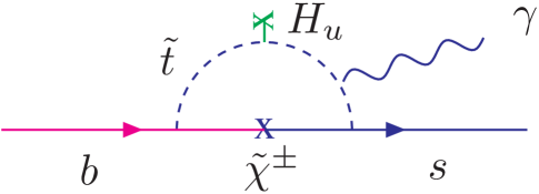
Figure 14: The one loop chargino contribution to the process $B\rightarrow X_{s}\gamma$ proportional to $\lambda_{t}$ and $\tan\beta$.

5.4.2 Flavor violating Higgs couplings at large $\tan\beta$

The MSSM has two Higgs doublets which at tree level satisfy the Glashow - Weinberg condition for natural flavor conservation. Up quarks get mass from $H_{u}$ and down quarks and charged leptons get mass from $H_{d}$. Thus when the fermion mass matrices are diagonalized (and neglecting small neutrino masses) the Higgs couplings to quarks and leptons are also diagonal. However, this is no longer true once SUSY is broken and radiative corrections are considered. In particular, for large values of $\tan\beta$ the coupling of $H_{u}$ to down quarks, via one loop corrections, results in significant flavor violating vertices for neutral and charged Higgs. These one loop corrections to the Higgs couplings contribute to an effective Lagrangian (Eqn. 5.4.2) [Blažek et al(1995), Chankowski and Pokorski (1997)]. The chargino contribution (Fig. 7) is proportional to the square of the up quark Yukawa matrix, which is not diagonal in the diagonal down quark mass basis. As a result, at one loop order, the down quark mass matrix is no longer diagonal (Eqn. 179). This leads to $\tan\beta$ enhanced corrections to down quark masses and to CKM matrix elements [Blažek et al(1995)]. Upon re-diagonalizing the down quark mass matrix we obtain the effective flavor violating Higgs - down quark Yukawa couplings given in Eqns. 5.4.2 and 181 [Chankowski and Pokorski (1997), Babu and Kolda (2000), Chankowski and Slawianowska (2001), Bobeth et al(2001), Huang et al(2001), Dedes et al(2001), Isidori and Retico (2001), Buras et al(2002,2003), Dedes and Pilaftsis (2003)].

$${\cal{L}}_{eff}^{ddH}= -\bar{d}_{Li}\ \lambda_{di}^{diag}\ d_{Ri}\ H_{d}^{0*}$$

$$-\bar{d}_{Li}\ \Delta\lambda_{d}^{ij}\ d_{Rj}\ H_{d}^{0*}$$

$$-\bar{d}_{Li}\ \delta\lambda_{d}^{ij}\ d_{Rj}\ H_{u}^{0}+{\rm h.c.}$$

$$m_{d}^{Diagonal} = V_{d}^{L}\ \left[\lambda_{d}^{diag}+\Delta\lambda_{d}+\delta\lambda_{d}\tan\beta\right]\ V_{d}^{R\dagger}\ \frac{v\cos\beta}{\sqrt{2}}$$ (179)

$${\cal{L}}_{FV}^{i\neq j}= -\frac{1}{\sqrt{2}}\bar{d^{\prime}}_{i}\left[F^{h}_{ij}\ P_{R}+F^{h*}_{ji}\ P_{L}\right]d^{\prime}_{j}\ h$$

$$-\frac{1}{\sqrt{2}}\bar{d^{\prime}}_{i}\left[F^{H}_{ij}\ P_{R}+F^{H*}_{ji}\ P_{L}\right]d^{\prime}_{j}\ H$$

$$-\frac{i}{\sqrt{2}}\bar{d^{\prime}}_{i}\left[F^{A}_{ij}\ P_{R}+F^{A*}_{ji}\ P_{L}\right]d^{\prime}_{j}\ A,$$

where

$$F^{h}_{ij} \simeq \delta\lambda_{d}^{ij}(1+\tan^{2}\beta)\cos\beta\ \cos(\alpha-\beta),$$ (181)

$$F^{H}_{ij} \simeq \delta\lambda_{d}^{ij}(1+\tan^{2}\beta)\cos\beta\ \sin(\alpha-\beta),$$

$$F^{A}_{ij} \simeq \delta\lambda_{d}^{ij}(1+\tan^{2}\beta)\ \cos\beta.$$

This leads to $\tan\beta$ enhanced flavor violating couplings for the neutral Higgs bosons. For example, the branching ratio $B(B_{s}\rightarrow\mu^{+}\mu^{-})$ is proportional to $\tan\beta^{4}$ and inversely proportional to the fourth power of the CP odd Higgs mass $m_{A}$ [Babu and Kolda (2000), Chankowski and Slawianowska (2001), Bobeth et al(2001), Huang et al(2001), Dedes et al(2001), Isidori and Retico (2001), Buras et al(2002,2003), Dedes and Pilaftsis (2003)], since the contributions of the two CP even Higgs bosons approximately cancel [Babu and Kolda (2000)]. The present D0 and CDF bounds constrain $m_{A}\geq 250$ GeV for $\tan\beta\sim 50$, although this result is somewhat model dependent [Dermíšek et al(2003)]. Note the D0 and CDF bounds from the Tevatron Run 2 now give $B(B_{s}\rightarrow\mu^{+}\mu^{-})<1.2\times 10^{-6}$ (CDF) [Lin (2003)] at 95% CL and $<1.6\times 10^{-6}$ (D0) [Kehoe (2003)]. An order of magnitude improvement will test large $\tan\beta$ SUSY for $m_{A}$ up to $\sim 500$ GeV [Dermíšek et al(2003)] (see Fig. 15).

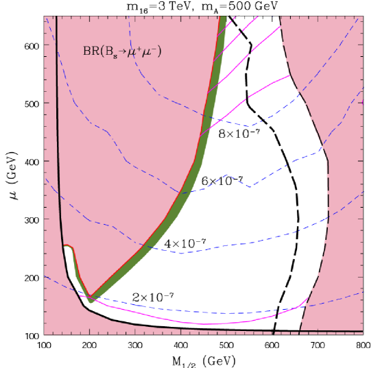
Figure 15: The dashed (blue) lines are contours for constant branching ratio $B(B_{s}\rightarrow\mu^{+}\mu^{-})$ as a function of $\mu,\ M_{1/2}$ for $m_{16}=3$ TeV. The green shaded region is consistent with the recent WMAP data for dark matter abundance of the neutralino LSP. The light shaded region in the lower left hand corner (separated by the solid line) is excluded by chargino mass limits, while the light shaded region in the upper left (right side) is excluded by a cosmological dark matter abundance which is too large (Higg mass which is too light).

6 SUSY Dark Matter

The two most popular dark matter candidates are axions or the LSP of SUSY. Both are well motivated cold dark matter candidates. There have been several recent studies of SUSY dark matter in light of the recent WMAP data. For these analyses and references to earlier works, see [Roszkowski et al(2003), Ellis et al(2003c,d,e,f), Chattopadhyay et al(2003)]. These calculations have been performed with different assumptions about soft SUSY breaking parameters, assuming the CMSSM boundary conditions at $M_{G}$ [Ellis et al(2003bc,d,f), Chattopadhyay et al(2003)] or arbitrary low energy scalar masses [Ellis et al(2003d)]. Soft SUSY breaking outside the realm of the CMSSM has also been considered. For example, soft breaking with non-universal Higgs masses have been analyzed recently by [Ellis et al(2003a,b), Roszkowski et al(2003)]. In the latter case, the soft SUSY breaking parameters consistent with SO(10) Yukawa unification were studied.

In the limit of large squark and slepton masses, it is important to have efficient mechanisms for dark matter annihilation. Most recent studies have focused on the neutralino LSP in the limit of large $\tan\beta$ and/or the focus point limit. In both cases there are new mechanisms for efficient neutralino annihilation. For large $\tan\beta\geq 40$ neutralino annihilation via direct s-channel neutral Higgs boson exchange dominates [Roszkowski et al(2001), Ellis et al(2001a,b)]. In this limit the CP even and odd Higgs bosons have large widths, due to their larger coupling to bottom quarks and $\tau$ leptons. In the focus point limit, on the other hand, the neutralino LSP is a mixed Higgsino - gaugino state. Thus it has more annihilation channels than the pure bino LSP case, valid for values of the universal scalar mass $m_{0}<$ TeV [Feng et al(2000c,2001)].

Direct detection [Ellis et al(2003b,e), Roszkowski et al(2003), Munoz (2003)] and/or indirect detection [Baer and Farrill (2003), de Boer et al(2003)] of neutralino dark matter has also been considered. In fact, [de Boer et al(2003)] suggests that some indirect evidence for SUSY dark matter already exists.

7 Open questions

It is beyond the scope of this review to comment on many other interesting topics affected by supersymmetric theories. Several effective mechanisms for generating the matter- anti-matter asymmetry of the universe have been suggested, including the Affleck-Dine mechanism [Affleck and Dine (1985)], which is purely a supersymmetric solution, or leptogenesis [Fukugita and Yanagida (1986)], which is not necessarily supersymmetric. There have also been many interesting studies of inflation in a SUSY context. Finally, we have only made passing reference to superstring theories and SUSY breaking mechanisms or fermion masses there.

Simple ”naturalness” arguments would lead one to believe that SUSY should have already been observed. On the other hand, “focus point” or “minimal SO(10) SUSY” regions of soft SUSY breaking parameter space extend to significantly heavier squark and slepton masses without giving up on “naturalness.” In both the “focus point” and “mSO₁₀SM” regions of parameter space we expect a light Higgs with mass of order $114-120$ GeV. Both ameliorate the SUSY flavor problem with heavy squark and slepton masses. They are nevertheless both surprisingly consistent with cosmological dark matter abundances. In addition, we have shown that the “mSO₁₀SM” satisfies Yukawa coupling unification with an inverted scalar mass hierarchy. Thus one finds first and second generation squarks and sleptons with mass of order several TeV, while gauginos and third generation squarks and sleptons are much ligher. In addition, it requires large values of $\tan\beta\sim 50$ resulting in enhanced flavor violation.

SUSY GUTs are the most natural extensions of the standard model, and thus they are the new “standard model” of particle physics. The mSUGRA (or CMSSM) boundary conditions at the GUT scale provide excellent fits to precision low energy electroweak data. SUSY GUTs, besides predicting gauge coupling unification, also provide a framework for resolving the gauge hierarchy problem and understanding fermion masses and mixing angles, including neutrinos. It also gives a natural dark matter candidate, and a framework for leptogenesis and inflation.

BUT there are two major challenges with any supersymmetric theory. We do not know how SUSY is spontaneously broken or the origin of the $\mu$ term. We are thus unable to predict the SUSY particle spectrum, which makes SUSY searches very difficult. Nevertheless, “naturalness” arguments always lead to some light SUSY sector, observable at the LHC, a light Higgs, with mass less than O(135 GeV), or observable flavor violating rates beyond that of the standard model. Assuming SUSY particles are observed at the LHC, then the fun has just begun. It will take many years to prove that it is really supersymmtry. Assuming SUSY is established, a SUSY desert from $M_{Z}$ to $M_{G}$ (or $M_{N}$) becomes highly likely. Thus precision measurements at the LHC or a Linear Collider will probe the boundary conditions at the very largest and fundamental scales of nature. With the additional observation of proton decay and/or precise GUT relations for sparticle masses, SUSY GUTs can be confirmed. Hence with experiments at TeV scale accelerators or in underground detectors for proton decay, neutrino oscillations or dark matter, the fundamental superstring physics can be probed. Perhaps then we may finally understand who ordered three families. It is thus no wonder why the elementary particle physics community is desperately seeking SUSY.

References

References

- [1] [] Affleck I and Dine M 1985 Nucl. Phys. B 249 361
- [2]
- [3] [] Albright C H and Barr S M 2000a Phys. Rev. Lett. 85 244 [arXiv:hep-ph/0002155]
- [4]
- [5] [] Albright C H and Barr S M 2000b Phys. Rev. D 62, 093008 (2000) [arXiv:hep-ph/0003251].
- [6]
- [7] [] Albright C H and Barr S M 2001 Phys. Rev. D64 073010 [arXiv:hep-ph/0104294]
- [8]
- [9] [] Ali A, Lunghi E, Greub C and Hiller G 2002 Phys. Rev. D 66 034002 [arXiv:hep-ph/0112300]
- [10]
- [11] [] Allanach B C, King S F, Leontaris G K and Lola S 1997 Phys. Lett. B 407 275 [arXiv:hep-ph/9703361]
- [12]
- [13] [] Altarelli G, Feruglio F and Masina I 2000 JHEP 0011 040 [arXiv:hep-ph/0007254]
- [14]
- [15] [] Altarelli G, Feruglio F 2001 Phys. Lett. B511 257 [arXiv:hep-ph/0102301]
- [16]
- [17] [] Altarelli G and Feruglio F 2003 [arXiv:hep-ph/0306265]
- [18]
- [19] [] Altarelli G, Feruglio F and Masina I 2003 JHEP 0301 035 [arXiv:hep-ph/0210342]
- [20]
- [21] [] Alvarez-Gaume L, Claudson M and Wise M B 1982 Nucl. Phys. B 207 96
- [22]
- [23] [] Alvarez-Gaume L, Polchinski J and Wise M B 1983 Nucl. Phys. B 221 495
- [24]
- [25] [] Amaldi U, de Boer W and Fürstenau H 1991 Phys. Lett. B260 447
- [26]
- [27] [] Ananthanarayan B, Lazarides G and Shafi Q 1991 Phys. Rev. D 44 1613
- [28]
- [29] [] Ananthanarayan B, Lazarides G and Shafi Q 1993 Phys. Lett. B 300 245
- [30]
- [31] [] Ananthanarayan B, Shafi Q and Wang X M 1994 Phys. Rev. D 50 5980
- [32]
- [33] [] Anderson G W and Castaño D J 1995 Phys. Lett. B 347 300
- [34]
- [35] [] Anderson G W, Raby S, Dimopoulos S and Hall L J 1993 Phys. Rev. D 47 3702 [arXiv:hep-ph/9209250]
- [36]
- [37] [] Anderson G, Raby S, Dimopoulos S, Hall L J and Starkman G D 1994 Phys. Rev. D 49 3660 [arXiv:hep-ph/9308333]
- [38]
- [39] [] Aoki S et al(JLQCD) 2000 Phys. Rev. D 62 014506
- [40]
- [41] [] Aoki Y et al(RBC) 2002 [arXiv:hep-lat/0210008]
- [42]
- [43] [] Appelquist T, Dobrescu B A, Ponton E and Yee H U 2001 Phys. Rev. Lett. 87 181802 [arXiv:hep-ph/0107056]
- [44]
- [45] [] Aranda A, Carone C D and Lebed R F 2000 Phys. Lett. B 474 170 [arXiv:hep-ph/9910392]
- [46]
- [47] [] Arkani-Hamed N, Cheng H C and Hall L J 1996 Phys. Rev. D54 2242 [arXiv:hep-ph/9601262]
- [48]
- [49] [] Arkani-Hamed N, Dimopoulos S and Dvali G R 1998 Phys. Lett. B 429 263 [arXiv:hep-ph/9803315]
- [50]
- [51] [] Aulakh C S, Bajc B, Melfo A, Senjanovic G and Vissani F 2003 [arXiv:hep-ph/0306242]
- [52]
- [53] [] Auto D, Baer H, Balazs C, Belyaev A, Ferrandis J and Tata X 2003 JHEP 0306, 023 [arXiv:hep-ph/0302155]
- [54]
- [55] [] Babu K S and Barr S M 1993 Phys. Rev. D 48 5354 [arXiv:hep-ph/9306242]
- [56]
- [57] [] Babu K S and Barr S M 2002 Phys. Rev. D 65 095009 [arXiv:hep-ph/0201130]
- [58]
- [59] [] Babu K S and Kolda C 2000 Phys. Rev. Letters84 228
- [60]
- [61] [] Babu K S and Mohapatra R N 1995 Phys. Rev. Lett.74 2418
- [62]
- [63] [] Babu K S, Pati J C and Wilczek F 2000 Nucl. Phys. B 566 33
- [64]
- [65] [] Babu K S and Strassler M J 1998 [arXiv:hep-ph/9808447]
- [66]
- [67] [] Baer H, Balazs C, Belyaev A and O’Farrill J 2003 JCAP 0309 007 [arXiv:hep-ph/0305191]
- [68]
- [69] [] Baer H, Balazs C, Mercadante P, Tata X and Wang Y 2001a Phys. Rev. D 63 015011 [arXiv:hep-ph/0008061]
- [70]
- [71] [] Baer H, Balazs C, Brhlik M, Mercadante P, Tata X and Wang Y 2001b Phys. Rev. D 64 015002 [arXiv:hep-ph/0102156]
- [72]
- [73] [] Baer H, Mercadante P and Tata X 2000 Phys. Lett. B 475 289 [arXiv:hep-ph/9912494]
- [74]
- [75] [] Baer H and Ferrandis J 2001 Phys. Rev. Lett. 87 211803
- [76]
- [77] [] Baer H and Farrill J O 2003 [arXiv:hep-ph/0312350]
- [78]
- [79] [] Bagger J, Dimopoulos S, Georgi H and Raby S 1984 Proceedings of the 5th Workshop on Grand Unification, Providence, RI, Apr 12-14, 1984
- [80]
- [81] [] Bagger J A, Feng J L and Polonsky N 1999 Nucl. Phys. B 563 3 [arXiv:hep-ph/9905292]
- [82]
- [83] [] Bagger J A, Feng J L, Polonsky N and Zhang R-J 2000 Phys. Lett. B 473 264 [arXiv:hep-ph/9911255]
- [84]
- [85] [] Bajc B, Perez P F and Senjanovic G 2002 Phys. Rev. D 66 075005 [arXiv:hep-ph/0204311]
- [86]
- [87] [] Bajc B, Senjanovic G and Vissani F 2003 Phys. Rev. Lett.90 051802 [arXiv:hep-ph/0210207]
- [88]
- [89] [] Banks T 1988 Nucl. Phys. B 303 172
- [90]
- [91] [] Banks T and Kaplunovsky V 1983 Nucl. Phys. B 211 529
- [92]
- [93] [] Barbieri R, Dvali G R and Hall L J 1996 Phys. Lett. B 377 76 [arXiv:hep-ph/9512388].
- [94]
- [95] [] Barbieri R, Ferrara S and Savoy C A 1982 Phys. Lett. B 119 343
- [96]
- [97] [] Barbieri R and Giudice G F 1988 Nucl. Phys. B 306 63
- [98]
- [99] [] Barbieri R and Hall L J 1997 Nuovo Cim. A 110 1 [arXiv:hep-ph/9605224]
- [100]
- [101] [] Barbieri R, Hall L J, Raby S and Romanino A 1997a Nucl. Phys. B 493 3
- [102]
- [103] [] Barbieri R, Hall L J and Romanino A 1997b Phys. Lett. B 401 47 [arXiv:hep-ph/9702315]
- [104]
- [105] [] Barbieri R, Hall L J and Romanino A 1999 Nucl. Phys. B 551 93 [arXiv:hep-ph/9812384]
- [106]
- [107] [] Barbieri R, Hall L J and Strumia A 1995a Nucl. Phys. B445 219 [arXiv:hep-ph/9501334]
- [108]
- [109] [] Barbieri R, Hall L J and Strumia A 1995b Nucl. Phys. B 449 437 [arXiv:hep-ph/9504373]
- [110]
- [111] [] Barbieri R and Strumia A 1998 Phys. Lett. B 433 63 hep-ph/9801353
- [112]
- [113] [] Barger V D, Berger M S and Ohmann P 1993 Phys. Rev. D 47 1093 [arXiv:hep-ph/9209232]
- [114]
- [115] [] Barger V, Marfatia D and Whisnant K 2003 Int. J. Mod. Phys. E 12 569 [arXiv:hep-ph/0308123]
- [116]
- [117] [] Barr S M and Dorsner I 2003 Phys. Lett. B 556 185 [arXiv:hep-ph/0211346]
- [118]
- [119] [] Berezhiani Z G 1983 Phys. Lett. B 129 99
- [120]
- [121] [] Berezhiani Z G 1985 Phys. Lett. B 150 177
- [122]
- [123] [] Berezhiani Z 1998 Phys. Lett. B 417 287 [arXiv:hep-ph/9609342]
- [124]
- [125] [] Berezhiani Z and Rossi A 2001 Nucl. Phys. B 594 113
- [126]
- [127] [] Berezinsky V, Bottino A, Ellis J R, Fornengo N, Mignola G and Scopel S 1996 Astropart. Phys. 5, 333 [arXiv:hep-ph/9603342]
- [128]
- [129] [] Binetruy P, Lavignac S and Ramond P 1996 Nucl. Phys. B477 353 [arXiv:hep-ph/9601243]
- [130]
- [131] [] Blažek T, Carena M, Raby S and Wagner C 1997a Nucl. Phys. Proc. Suppl. A 52 133 [arXiv:hep-ph/9608273]
- [132]
- [133] [] Blažek T, Carena M, Raby S and Wagner C E M 1997b Phys. Rev. D 56 6919 [arXiv:hep-ph/9611217]
- [134]
- [135] [] Blažek T, Dermíšek R and Raby S 2002a Phys. Rev. Lett. 88 111804
- [136]
- [137] [] Blažek T, Dermíšek R and Raby S 2002b Phys. Rev. D 65 115004 [arXiv:hep-ph/0201081]
- [138]
- [139] [] Blažek T, Pokorski S and Raby S 1995 Phys. Rev. D52 4151
- [140]
- [141] [] Blažek T and Raby S 1999 Phys. Rev. D 59 095002 [arXiv:hep-ph/9712257]
- [142]
- [143] [] Blažek T, Raby S and Tobe K 1999 Phys. Rev. D 60 113001 [arXiv:hep-ph/9903340]
- [144]
- [145] [] Blažek T, Raby S and Tobe K 2000 Phys. Rev. D 62 055001 [arXiv:hep-ph/9912482]
- [146]
- [147] [] Bobeth C, Ewerth T, Kruger F and Urban J 2001 Phys. Rev. D 64 074014 [arXiv:hep-ph/0104284]
- [148]
- [149] [] Bobeth C, Gambino P, Gorbahn M and Haisch U 2003 [arXiv:hep-ph/0312090]
- [150]
- [151] [] Borzumati F and Masiero A 1986 Phys. Rev. Lett.57 961
- [152]
- [153] [] Brodsky S J, Ellis J, Hagelin J S and Sachradja C 1984 Nucl. Phys. B238 561
- [154]
- [155] [] Buchmuller W 2001 hep-ph/0107153
- [156]
- [157] [] Buchmuller W, Di Bari P and Plumacher M 2003 Nucl. Phys. B 665 445 [arXiv:hep-ph/0302092]
- [158]
- [159] [] Buras A J, Chankowski P H, Rosiek J and Slawianowska L 2002 Phys. Lett. B 546 96 [arXiv:hep-ph/0207241]
- [160]
- [161] [] Buras A J, Chankowski P H, Rosiek J and Slawianowska L 2003 Nucl. Phys. B659 3 [arXiv:hep-ph/0210145]
- [162]
- [163] [] Carena M et al1994 Nucl. Phys. B426 269
- [164]
- [165] [] Carena M et al1995 Phys. Lett. B355 209
- [166]
- [167] [] Carena M, Garcia D, Nierste U and Wagner C E M 2001 Phys. Lett. B 499 141 [arXiv:hep-ph/0010003]
- [168]
- [169] [] Carena M, Quiros M and Wagner C E M 1996 Nucl. Phys. B461 407
- [170]
- [171] [] Carone C D, Hall L J and Murayama H 1996 Phys. Rev. D 53 6282 [arXiv:hep-ph/9512399]
- [172]
- [173] [] Carone C D and Lebed R F 1999 Phys. Rev. D 60 096002
- [174]
- [175] [] Casas J A, Espinosa J R and Navarro I 2003 “Large mixing angles for neutrinos from infrared fixed points,” JHEP0309 048 [hep-ph/0306243]
- [176]
- [177] [] Casas J A, Espinosa J R, Quiros M and Riotto A 1995 Nucl. Phys. B436 3; Erratum 1995 Nucl. Phys. B439 466
- [178]
- [179] [] Casas J A and Ibarra A 2001 Nucl. Phys. B 618 171 [arXiv:hep-ph/0103065]
- [180]
- [181] [] Chamseddine A H, Arnowitt R and Nath P 1982 Phys. Rev. Lett. 49 970
- [182]
- [183] [] Chankowski P H, Ellis J R and Pokorski S 1997 Phys. Lett. B 423 327 [arXiv:hep-ph/9712234]
- [184]
- [185] [] Chankowski P H, Ellis J R, Olechowski M and Pokorski S 1999 Nucl. Phys. B 544 39 [arXiv:hep-ph/9808275]
- [186]
- [187] [] Chankowski P H and Pokorski S 1997, in Perspectives on supersymmetry, Kane, G.L. (ed.), p. 402, World Scientific [arXiv:hep-ph/9707497]
- [188]
- [189] [] Chankowski P H and Slawianowska L 2001 Phys. Rev. D63 054012 [arXiv:hep-ph/0008046]
- [190]
- [191] [] Chattopadhyay U, Corsetti A and Nath P 2003 Phys. Rev. D 68 035005 [arXiv:hep-ph/0303201]
- [192]
- [193] [] Chattopadhyay U and Nath P 1996 Phys. Rev. D 53 1648 [arXiv:hep-ph/9507386]
- [194]
- [195] [] Choudhury S R and Gaur N 1999 Phys. Lett. B451 86 [arXiv:hep-ph/9810307]
- [196]
- [197] [] Chen M C and Mahanthappa K T 2003 Phys. Rev. D68 017301
- [198]
- [199] [] Chen M C and Mahanthappa K T 2003 [arXiv:hep-ph/0305088]
- [200]
- [201] [] Claudson M, Wise M and Hall L J 1982 Nucl. Phys. B195 297
- [202]
- [203] [] Chadha S and Daniel M 1983 Nucl. Phys. B229 105
- [204]
- [205] [] Ciuchini M, Degrassi G, Gambino P and Giudice G F 1998 Nucl. Phys. B 534 3 [arXiv:hep-ph/9806308]
- [206]
- [207] [] Contino R, Pilo L, Rattazzi R and Trincherini E 2002 Nucl. Phys. B 622 227 [arXiv:hep-ph/0108102]
- [208]
- [209] [] Davidson S and Ibarra A 2001 JHEP0109 013 [arXiv:hep-ph/0104076]
- [210]
- [211] [] Davier M, Eidelman S, Hocker A and Zhang Z 2003 Eur. Phys. J. C 31 503 [arXiv:hep-ph/0308213]
- [212]
- [213] [] de Boer W, Herold M, Sander C and Zhukov V 2003 [arXiv:hep-ph/0309029]
- [214]
- [215] [] de Boer W and Sanders C 2003 [arXiv:hep-ph/0307049]
- [216]
- [217] [] de Carlos B and Casas J A 1993 Phys. Lett. B 309 320
- [218]
- [219] [] Dedes A, Dreiner H K and Nierste U 2001 [arXiv:hep-ph/0108037]
- [220]
- [221] [] Dedes A and Pilaftsis A 2003 Phys. Rev. D67 015012 [arXiv:hep-ph/0209306]
- [222]
- [223] [] Degrassi G, Heinemeyer S, Hollik W, Slavich P and Weiglein G 2003 Eur. Phys. J. C 28 133 [arXiv:hep-ph/0212020]
- [224]
- [225] [] Demir D, Lebedev O, Olive K A, Pospelov M and Ritz A 2003 [arXiv:hep-ph/0311314]
- [226]
- [227] [] Dermíšek R 2001 Published in *Dubna 2001, Supersymmetry and unification of fundamental interactions* 284-286 [arXiv:hep-ph/0108249]
- [228]
- [229] [] Dermíšek R, Mafi A and Raby S 2001 Phys. Rev. D 63 035001 [arXiv:hep-ph/0007213]
- [230]
- [231] [] Dermíšek R and Raby S 2000 Phys. Rev. D 62 015007 [arXiv:hep-ph/9911275]
- [232]
- [233] [] Dermíšek R, Raby S, Roszkowski L and Ruiz De Austri R 2003 JHEP 0304 037 [arXiv:hep-ph/0304101]
- [234]
- [235] [] Dimopoulos S 1983 Phys. Lett. B129 417
- [236]
- [237] [] Dimopoulos S, Dine M, Raby S and Thomas S 1996 Phys. Rev. Lett. 76 3494 [arXiv:hep-ph/9601367]
- [238]
- [239] [] Dimopoulos S and Georgi H 1981 Nucl. Phys. B 193 150
- [240]
- [241] [] Dimopoulos S and Giudice G F 1995 Phys. Lett. B 357 573 [arXiv:hep-ph/9507282]
- [242]
- [243] [] Dimopoulos S and Hall L J 1995 Phys. Lett. B 344 185 [arXiv:hep-ph/9411273]
- [244]
- [245] [] Dimopoulos S, Hall L J and Raby S 1992 Phys. Rev. Lett. 68 1984; ibid., Phys. Rev. D 45 4192
- [246]
- [247] [] Dimopoulos S and Pomarol A 1995 Phys. Lett. B 353 222 [arXiv:hep-ph/9502397]
- [248]
- [249] [] Dimopoulos S and Raby S 1981 Nucl. Phys. B 192 353
- [250]
- [251] [] Dimopoulos S and Raby S 1983 Nucl. Phys. B 219 479
- [252]
- [253] [] Dimopoulos S, Raby S, and Wilczek F 1981 Phys. Rev. D 24 1681
- [254]
- [255] [] Dimopoulos S, Raby S and Wilczek F 1982 Phys. Lett. 112B 133
- [256]
- [257] [] Dimopoulos S, Raby S, and Wilczek F 1991 Phys. Today 44N10 25
- [258]
- [259] [] Dimopoulos S and Sutter D W 1995 Nucl. Phys. B 452 496 [arXiv:hep-ph/9504415]
- [260]
- [261] [] Dine M, Fischler W and Srednicki M 1981 Nucl. Phys. B 189 575
- [262]
- [263] [] Dine M, Fischler W 1982 Phys. Lett. B 110 227
- [264]
- [265] [] Dine M, Leigh R and Kagan A 1993 Phys. Rev. D48 4269
- [266]
- [267] [] Dine M and Nelson A E 1993 Phys. Rev. D 48 1277 [arXiv:hep-ph/9303230]
- [268]
- [269] [] Dine M, Nelson A E and Shirman Y 1995 Phys. Rev. D 51 1362 [arXiv:hep-ph/9408384]
- [270]
- [271] [] Dine M, Nelson A E, Nir Y and Shirman Y 1996 Phys. Rev. D 53 2658 [arXiv:hep-ph/9507378]
- [272]
- [273] [] Dine M, Nir Y and Shadmi Y 2002 Phys. Rev. D 66 115001 [arXiv:hep-ph/0206268]
- [274]
- [275] [] Dixon L J, Harvey J A, Vafa C and Witten E 1985 Nucl. Phys. B261 678
- [276]
- [277] [] Dixon L J, Harvey J A, Vafa C and Witten E 1986 Nucl. Phys. B274 285 (1986)
- [278]
- [279] [] Dreiner H K, Murayama H and Thormeier M 2003 [arXiv:hep-ph/0312012]
- [280]
- [281] [] Dudas E, Pokorski S and Savoy C A 1995 Phys. Lett. B356 45
- [282]
- [283] [] Dudas E, Pokorski S and Savoy C A 1996 Phys. Lett. B369 255
- [284]
- [285] [] Einhorn M B and Jones D R 1982 Nucl. Phys. B 196 475
- [286]
- [287] [] Elwood J K, Irges N, and Ramond P 1997 Phys. Lett. B413 322 [arXiv:hep-ph/9705270]
- [288]
- [289] [] Elwood J K, Irges N, and Ramond P 1998 Phys. Rev. Lett.81 5064 [arXiv:hep-ph/9807228]
- [290]
- [291] [] Ellis J, Falk T, Ganis G, Olive K A and Srednicki M 2001b Phys. Lett. B510 (236)
- [292]
- [293] [] Ellis J R, Hisano J, Raidal M and Shimizu Y 2002 Phys. Rev. D 66 115013 [arXiv:hep-ph/0206110]
- [294]
- [295] [] Ellis J, Kelly S and Nanopoulos D V 1991 Phys. Lett. B 260 131
- [296]
- [297] [] Ellis J, Nanopoulos D V and Rudaz S 1982 Nucl. Phys. B 202 43
- [298]
- [299] [] Ellis J, Nanopoulos D V and Olive K A 2001a Phys. Lett. B508 (65)
- [300]
- [301] [] Ellis J R, Enqvist K, Nanopoulos D V and Zwirner F 1986 Nucl. Phys. B 276 14
- [302]
- [303] [] Ellis J R, Falk T, Olive K A and Santoso Y 2003a Nucl. Phys. B 652, 259 (2003) [arXiv:hep-ph/0210205].
- [304]
- [305] [] Ellis J R, Ferstl A, Olive K A and Santoso Y 2003b Phys. Rev. D 67 123502 [arXiv:hep-ph/0302032]
- [306]
- [307] [] Ellis J R, Olive K A, Santoso Y and Spanos V C 2003c Phys. Lett. B 565 176 [arXiv:hep-ph/0303043]
- [308]
- [309] [] Ellis J R, Olive K A, Santoso Y and Spanos V C 2003d Phys. Lett. B 573, 162 (2003) [arXiv:hep-ph/0305212].
- [310]
- [311] [] Ellis J R, Olive K A, Santoso Y and Spanos V C 2003e [arXiv:hep-ph/0308075]
- [312]
- [313] [] Ellis J R, Olive K A, Santoso Y and Spanos V C 2003f [arXiv:hep-ph/0310356]
- [314]
- [315] [] Ellis J R, Ridolfi G and Zwirner F 1991 Phys. Lett. B 257 83
- [316]
- [317] [] Espinosa J R and Zhang R J (2000a) JHEP0003 026
- [318]
- [319] [] Espinosa J R and Zhang R J (2000b) Nucl. Phys. B586 3
- [320]
- [321] [] Eyal G 1998 Phys. Lett. B 441 191 [arXiv:hep-ph/9807308]
- [322]
- [323] [] Faraggi A E and Pati J C 1998 Nucl. Phys. B 526 21
- [324]
- [325] [] Farrar G and Fayet P 1978 Phys. Lett. B76 575
- [326]
- [327] [] Fayet P and Ferrara S 1977 Phys. Rept. 32 249
- [328]
- [329] [] Feng J L and Moroi T 2000 Phys. Rev. D 61 095004 [arXiv:hep-ph/9907319]
- [330]
- [331] [] Feng J L, Matchev K T and Moroi T 2000a Phys. Rev. Lett. 84 2322 [arXiv:hep-ph/9908309]
- [332]
- [333] [] Feng J L, Matchev K T and Moroi T 2000b Phys. Rev. D 61 075005 [arXiv:hep-ph/9909334]
- [334]
- [335] [] Feng J L, Matchev K T and Wilczek F 2000c Phys. Lett. B 482 388 [arXiv:hep-ph/0004043]
- [336]
- [337] [] Feng J L, Matchev K T and Wilczek F 2001 Phys. Rev. D63 (045024)
- [338]
- [339] [] Feng J L, Matchev K T 2001 Phys. Rev. D 63 095003 [arXiv:hep-ph/0011356]
- [340]
- [341] [] Frampton P H, Glashow S L and Yanagida T 2002 Phys. Lett. B548 119 [arXiv:hep-ph/0208157]
- [342]
- [343] [] Frampton P H and Kephart T W 1995a Phys. Rev. D51 1
- [344]
- [345] [] Frampton P H and Kephart T W 1995b Int. J. Mod. Phys. A 10 4689
- [346]
- [347] [] Frampton P H and Kong O C W 1996 Phys. Rev. Lett. 77 1699 [arXiv:hep-ph/9603372]
- [348]
- [349] [] Frampton P H and Rasin A 2000 Phys. Lett. B 478 424 [arXiv:hep-ph/9910522]
- [350]
- [351] [] Fritzsch H and Minkowski P 1975 Ann. Phys. 93 193
- [352]
- [353] [] Froggatt C D and Nielsen H B 1979 Nucl. Phys. B147 277
- [354]
- [355] [] Fukugita M and Yanagida T 1986 Phys. Lett. B 174 45
- [356]
- [357] [] Gabbiani F, Gabrieli E, Masiero A and Silvestrini L 1996 Nucl. Phys. B477 321 [arXiv:hep-ph/9604387]
- [358]
- [359] [] Gavela M B, King S F, Sachrajda C T, Martinelli G, Paciello M L, and Taglienti B 1989 Nucl. Phys. B 312 269
- [360]
- [361] [] Gell-Mann M, Ramond P and Slansky R 1979 Supergravity, [Sept. 27-29 1979], eds. D. Freedman et al., (North Holland, 1980, Amsterdam)
- [362]
- [363] [] Georgi H 1975 Particles and Fields, Proceedings of the APS Div. of Particles and Fields, ed C. Carlson, p. 575
- [364]
- [365] [] Georgi G 1986 Phys. Lett. B 169 231
- [366]
- [367] [] Georgi H and Glashow S L 1974 Phys. Rev. Lett. 32 438
- [368]
- [369] [] Georgi H and Jarlskog C 1979 Phys. Lett. B 86 297
- [370]
- [371] [] Georgi H, Quinn H R and Weinberg S 1974 Phys. Rev. Lett. 33 451
- [372]
- [373] [] Georgi H and Nanopoulos D V 1979 Nucl. Phys. B 159 16
- [374]
- [375] [] Girardello L and Grisaru M T 1982 Nucl. Phys. B 194 65
- [376]
- [377] [] Giudice G F, Notari A, Raidal M, Riotto A and Strumia A 2003 [arXiv:hep-ph/0310123]
- [378]
- [379] [] Giudice G F and Rattazzi R 1999 Phys. Rept. 322 419 [arXiv:hep-ph/9801271]
- [380]
- [381] [] Glashow S L 1979 Quarks and Leptons, Carg‘ese, [July 9-29,1979], eds. M. L evy, et al., (Plenum, 1980, New York), p. 707
- [382]
- [383] [] Goh H S, Mohapatra R N and Ng S P 2003 Phys. Lett. B 570 215 [arXiv:hep-ph/0303055]
- [384]
- [385] [] Gonzalez-Garcia M C and Pena-Garay C 2003 Phys. Rev. D 68 093003 [arXiv:hep-ph/0306001]
- [386]
- [387] [] Goto T and Nihei T 1999 Phys. Rev. D 59 115009 [arXiv:hep-ph/9808255]
- [388]
- [389] [] Grinstein B 1982 Nucl. Phys. B 206 387
- [390]
- [391] [] Haber H E and Hempfling R 1993 Phys. Rev. D48 4280
- [392]
- [393] [] Haber H E, Hempfling R and Hoang A H 1997 Z. Phys. C 75 539 [arXiv:hep-ph/9609331]
- [394]
- [395] [] Hagiwara K, Martin A D, Nomura D and Teubner T 2003 [arXiv:hep-ph/0312250]
- [396]
- [397] [] Hall L J, Kostelecky V A and Raby S 1986 Nucl. Phys. B 267 415
- [398]
- [399] [] Hall L J, Lykken J and Weinberg S 1983 Phys. Rev. D 27 2359
- [400]
- [401] [] Hall L J and Murayama H 1995 Phys. Rev. Lett.75 3985
- [402]
- [403] [] Hall L J and Nomura Y 2001 Phys. Rev. D 64 055003 [arXiv:hep-ph/0103125]
- [404]
- [405] [] Hall L J and Nomura Y 2002a Phys. Rev. D 65 125012 [arXiv:hep-ph/0111068]
- [406]
- [407] [] Hall L J and Nomura Y 2002b Phys. Rev. D66 075004 [arXiv:hep-ph/0205067]
- [408]
- [409] [] Hall L J and Randall L 1990 Phys. Rev. Lett.65 2939
- [410]
- [411] [] Hall L J and Rasin A 1993 Phys. Lett. B 315 164 [arXiv:hep-ph/9303303]
- [412]
- [413] [] Hall L J, Rattazzi R and Sarid U 1994 Phys. Rev. D50 7048
- [414]
- [415] [] Hamzaoui C, Pospelov M and Toharia M 1999 Phys. Rev. D59 095005
- [416]
- [417] [] Hara Y, Itoh S, Iwasaki Y and Yoshie T 1986 Phys. Rev. D34 3399
- [418]
- [419] [] Harvey J, Ramond P and Reiss D B 1980 Phys. Lett. B 92 309
- [420]
- [421] [] Harvey J, Ramond P and Reiss D B 1982 Nucl. Phys. B 199 223
- [422]
- [423] [] Hebecker A and March-Russell J 2002 Phys. Lett. B539 119 [arXiv:hep-ph/0204037]
- [424]
- [425] [] Hempfling R 1994 Phys. Rev. D49 6168
- [426]
- [427] [] Hisano J, Moroi T, Tobe K, Yamaguchi M and Yanagida T 1995 Phys. Lett. B 357 579 [arXiv:hep-ph/9501407]
- [428]
- [429] [] Hisano J, Moroi T, Tobe K and Yamaguchi M 1996 Phys. Rev. D 53 2442 [arXiv:hep-ph/9510309]
- [430]
- [431] [] Hisano J and Tobe K 2001 Phys. Lett. B 510 197 [arXiv:hep-ph/0102315]
- [432]
- [433] [] Huang C S and Yan Q S 1998 Phys. Lett. B442 209 [arXiv:hep-ph/9803366]
- [434]
- [435] [] Huang C S, Liao W and Yan Q S (1999) Phys. Rev. D59 011701 [arXiv:hep-ph/9803460]
- [436]
- [437] [] Huang C S, Liao W, Yan Q S and Zhu S H 2001 Phys. Rev. D63 114021 [Erratum: Phys. Rev. D64 (2001), 059902]
- [438]
- [439] [] Ibañez L E 1982 Phys. Lett. B 118 73
- [440]
- [441] [] Ibañez L E and Lopez C 1983 Phys. Lett. B 126 54
- [442]
- [443] [] Ibañez L E and Lopez C 1984 Nucl. Phys. B 233 511
- [444]
- [445] [] Ibañez L and Ross G G 1981 Phys. Lett. B 105 439
- [446]
- [447] [] Ibañez L and Ross G G 1982 Phys. Lett. B 110 215
- [448]
- [449] [] Ibañez L and Ross G G 1992 “Perspectives on Higgs physics” Kane G L (ed.) 229-275 [arXiv:hep-ph/9204201]
- [450]
- [451] [] Inoue K, Kakuto A, Komatsu H and Takeshita S 1982 Prog. Theor. Phys. 67 1889
- [452]
- [453] [] Irges N, Lavignac S and Ramond P 1998 Phys. Rev. D58 035003 [arXiv:hep-ph/9802334]
- [454]
- [455] [] Isidori G and Retico A 2001 [arXiv:hep-ph/0110121]
- [456]
- [457] [] Jeannerot R, Khalil S and Lazarides G 2001 Phys. Lett. B 506 344 [arXiv:hep-ph/0103229]
- [458]
- [459] [] Jung C K 2002 Brookhaven National Lab preprint, UNO 02-BNL
- [460]
- [461] [] Kakizaki M and Yamaguchi M 2002 JHEP0206 032 [arXiv:hep-ph/0203192]
- [462]
- [463] [] Kane G L, Kolda C F, Roszkowski L and Wells J D 1994 Phys. Rev. D 49 6173 [arXiv:hep-ph/9312272]
- [464]
- [465] [] Kane G L, Nelson B D, Wang T T and Wang L T (2003) [arXiv:hep-ph/0304134]
- [466]
- [467] [] Kaplan D B and Schmaltz M 1994 Phys. Rev. D49 3741 [arXiv:hep-ph/9311281]
- [468]
- [469] [] Kawamura Y 2001a Prog. Theor. Phys.105 999 [arXiv:hep-ph/0012125]
- [470]
- [471] [] Kawamura Y 2001b Prog. Theor. Phys.105 691 [arXiv:hep-ph/0012352]
- [472]
- [473] [] Kehoe R 2003 http://www-clued0.fnal.gov/ kehoe/physics/fermiwc.pdf
- [474]
- [475] [] Kim H D and Raby S 2003 JHEP 0301 056 [arXiv:hep-ph/0212348]
- [476]
- [477] [] Kim H D, Raby S and Schradin L (2004) [arXiv:hep-ph/0401169]
- [478]
- [479] [] King S F 1998 Phys. Lett. B 439 350 [arXiv:hep-ph/9806440]
- [480]
- [481] [] King S F 2000 Nucl. Phys. B 576 85 [arXiv:hep-ph/9912492]
- [482]
- [483] [] King S F 2003 [arXiv:hep-ph/0310204]
- [484]
- [485] [] King S F and Ross G G 2003 Phys. Lett. B574 239 [arXiv:hep-ph/0307190]
- [486]
- [487] [] Kitano R and Mimura Y 2001 Phys. Rev. D63 016008
- [488]
- [489] [] Klebanov I R and Witten E 2003 Nucl. Phys. B 664 3 [arXiv:hep-th/0304079]
- [490]
- [491] [] Langacker P and Luo M 1991 Phys. Rev. D 44 817
- [492]
- [493] [] Lavignac S, Masina I and Savoy C A 2001 Phys. Lett. B520 269 [arXiv:hep-ph/0106245]
- [494]
- [495] [] Lavignac S, Masina I and Savoy C A 2002 Nucl. Phys. B633 139 [arXiv:hep-ph/0202086]
- [496]
- [497] [] LEP2 (2003), Barate R et al. [ALEPH Collaboration], Phys. Lett. B565 61 [arXiv:hep-ex/0306033]
- [498]
- [499] [] Leontaris G K, Tamvakis K and Vergados J D 1986 Phys. Lett. B171 412
- [500]
- [501] [] Leurer M, Nir Y and Seiberg N 1993 Nucl. Phys. B398 319
- [502]
- [503] [] Leurer M, Nir Y and Seiberg N 1994 Nucl. Phys. B420 319468
- [504]
- [505] [] Lin, C-J S 2003 (CDF Collaboration) Beauty 2003 Conference, Pittsburgh PA
- [506]
- [507] [] Lola S and Ross G G 1999 Nucl. Phys. B 553 81 [arXiv:hep-ph/9902283]
- [508]
- [509] [] Lucas V and Raby S 1996 Phys. Rev. D 54 2261 [arXiv:hep-ph/9601303]
- [510]
- [511] [] Lucas V and Raby S 1997 Phys. Rev. D 55 6986 [arXiv:hep-ph/9610293]
- [512]
- [513] [] Lunghi E, Masiero A, Scimemi I and Silvestrini L 2000 Nucl. Phys. B 568 120 [arXiv:hep-ph/9906286]
- [514]
- [515] [] Maekawa N 2001 Prog. Theor. Phys.106 401
- [516]
- [517] [] Maltoni M, Schwetz T, Tortola M A and Valle J W F (2003) Phys. Rev. D68, 113010 [arXiv:hep-ph/0309130]
- [518]
- [519] [] Marciano W J and Senjanovic G 1982 Phys. Rev. D 25 3092
- [520]
- [521] [] Masiero A, Nanopoulos D V, Tamvakis K and Yanagida T 1982 Phys. Lett. B 115 380
- [522]
- [523] [] Masiero A, Vempati S K and Vives O 2003 Nucl. Phys. B 649 189 [arXiv:hep-ph/0209303]
- [524]
- [525] [] Matalliotakis D and Nilles H P 1995 Nucl. Phys. B435 115
- [526]
- [527] [] Melnikov K and Vainshtein A 2003 [arXiv:hep-ph/0312226]
- [528]
- [529] [] Misiak M, Pokorski S and Rosiek J 1998 Adv. Ser. Direct. High Energy Phys.15 795 [arXiv:hep-ph/9703442]
- [530]
- [531] [] Mohapatra R N, Parida M K and Rajasekaran G 2003 [arXiv:hep-ph/0301234]
- [532]
- [533] [] Mohapatra R N and Senjanovic G 1980 Phys. Rev. Lett.44 912
- [534]
- [535] [] Moroi T 1996 Phys. Rev. D 53 6565 [Erratum-ibid. D 56, 4424 (1997)] [arXiv:hep-ph/9512396]
- [536]
- [537] [] Muon (g - 2) Collaboration, G. W. Bennett et al. 2002 Phys. Rev. Lett.89 101804, Erratum-ibid. 89 (2002) 129903
- [538]
- [539] [] Munoz C 2003 [arXiv:hep-ph/0312321]
- [540]
- [541] [] Murayama H, Olechowski M and Pokorski S 1996 Phys. Lett. B371 57
- [542]
- [543] [] Murayama H and Pierce A 2002 Phys. Rev. D 65 055009 [arXiv:hep-ph/0108104]
- [544]
- [545] [] Nath P and Arnowitt R 1997 Phys. Rev. D 56 2820 [arXiv:hep-ph/9701301]
- [546]
- [547] [] Nilles H P, Srednicki M and Wyler D 1983 Phys. Lett. B 120 346
- [548]
- [549] [] Nir Y and Seiberg N 1993 Phys. Lett. B309 337
- [550]
- [551] [] Nomura Y 2002 Phys. Rev. D 65 085036 [arXiv:hep-ph/0108170]
- [552]
- [553] [] Nomura Y, Smith D R and Weiner N 2001 Nucl. Phys. B 613 147 [arXiv:hep-ph/0104041]
- [554]
- [555] [] Nomura Y and Yanagida T 1999 Phys. Rev. D 59 017303 [arXiv:hep-ph/9807325]
- [556]
- [557] [] Okada Y, Yamaguchi M and Yanagida T 1991 Prog. Theor. Phys. 85 1
- [558]
- [559] [] Olechowski M and Pokorski S 1988 Phys. Lett. B214 393
- [560]
- [561] [] Olechowski M and Pokorski S 1995 Phys. Lett. B344 201
- [562]
- [563] [] Ovrut B A and Wess J 1982 Phys. Lett. B 112 347
- [564]
- [565] [] Paschos E A 2003 [arXiv:hep-ph/0308261]
- [566]
- [567] [] Pati J C and Salam A 1973a Phys. Rev. D 8 1240
- [568]
- [569] [] Pati J C and Salam A 1973b Phys. Rev. Lett.31 661
- [570]
- [571] [] Pati J C and Salam A 1974 Phys. Rev. D10 275
- [572]
- [573] [] Pierce D et al1997 Nucl. Phys. B491 3
- [574]
- [575] [] Pokorski S 1990 Nucl. Phys. B 13 (Proc. Supp.) 606
- [576]
- [577] [] Polchinski J and Susskind L 1982 Phys. Rev. D 26 3661
- [578]
- [579] [] Polonsky N and Pomarol A 1995 Phys. Rev. D51 6532
- [580]
- [581] [] Polony J 1977 Budapest preprint KFKI-1977-93 (unpublished)
- [582]
- [583] [] Pomarol A and Dimopoulos S 1995 Nucl. Phys. B 453 83 [arXiv:hep-ph/9505302]
- [584]
- [585] [] Pomarol A and Tommasini D 1996 Nucl. Phys. B 466 3 [arXiv:hep-ph/9507462]
- [586]
- [587] [] Pouliot P and Seiberg N 1993 Phys. Lett. B318 169
- [588]
- [589] [] Raby S 1995 Published in Trieste HEP Cosmology 1994:0126-180 [arXiv:hep-ph/9501349]
- [590]
- [591] [] Raby S 2001 Proceedings of Higgs & SUSY, March 2001, Orsay, France http://www.lal.in2p3.fr/actualite/conferences/higgs2001/slides/; Published in *Dubna 2001, Supersymmetry and unification of fundamental interactions* 168-176 [arXiv:hep-ph/0110203]
- [592]
- [593] [] Raby S 2002a in K. Hagiwara et al. [Particle Data Group Collaboration] Phys. Rev. D 66 010001
- [594]
- [595] [] Raby S 2002b Published in the proceedings of SUSY’02 [arXiv:hep-ph/0211024]
- [596]
- [597] [] Raby S 2003 Phys. Lett. B561 119
- [598]
- [599] [] Raidal M and Strumia A 2003 Phys. Lett. B 553 72 [arXiv:hep-ph/0210021]
- [600]
- [601] [] Rattazzi R and Sarid U 1996 Phys. Rev. D53 1553
- [602]
- [603] [] Roberts R G, Romanino A, Ross G G and Velasco-Sevilla L 2001 Nucl. Phys. B 615 358 [arXiv:hep-ph/0104088]
- [604]
- [605] [] Romanino A and Strumia A 2000 Phys. Lett. B 487 165 [arXiv:hep-ph/9912301]
- [606]
- [607] [] Ross G G and Velasco-Sevilla L 2003 Nucl. Phys. B653 3
- [608]
- [609] [] Roszkowski L, Ruiz de Austri, R and Nihei T 2001 JHEP 0108 024 [arXiv:hep-ph/0106334]
- [610]
- [611] [] Sakai N 1981 Z. Phys. C11 153
- [612]
- [613] [] Sakai N and Yanagida T 1982 Nucl. Phys. B197, 533
- [614]
- [615] [] Shafi Q and Ananthanarayan B 1991 ICTP Summer School lectures
- [616]
- [617] [] Shafi Q and Tavartkiladze Z 2000 Phys. Lett. B 487 145
- [618]
- [619] [] Strumia A 1999 hep-ph/9904247
- [620]
- [621] [] Tobe K and Wells J D 2003 Nucl. Phys. B 663 123 [arXiv:hep-ph/0301015]
- [622]
- [623] [] Weinberg S 1982 Phys. Rev. D26 287
- [624]
- [625] [] Weisskopf V 1939 Phys. Rev. 56 72
- [626]
- [627] [] Witten E 1981 Nucl. Phys. B 188 513
- [628]
- [629] [] Witten E 2002 Published in *Hamburg 2002, Supersymmetry and unification of fundamental interactions, vol. 1 472-491 [arXiv:hep-ph/0201018]
- [630]
- [631] [] Yanagida T 1979 Proceedings of the Workshop on the unified theory and the baryon number of the universe, [Feb. 13-14, 1979], eds. O. Sawada and A. Sugamoto (Tsukuba,1979) p.95
- [632]
- [633] [] Zhang R J (1999) Phys. Lett. B447 89
- [634]