Constraining neutrino magnetic moment with solar and reactor neutrino data

Abstract:

We use solar neutrino data to derive stringent bounds on Majorana neutrino transition moments (TMs). Such moments, if present, would contribute to the neutrino–electron scattering cross section and hence alter the signal observed in Super-Kamiokande. Using the latest solar neutrino data, combined with the results of the reactor experiment KamLAND, we perform a simultaneous fit of the oscillation parameters and TMs. Furthermore, we show how the inclusion of data from the reactor experiments Rovno, TEXONO and MUNU in our analysis improves significantly the current constraints on TMs. Finally, we perform a simulation of the future Borexino experiment and show that it will improve the bounds from today’s data by order of magnitude.

1 Introduction

Present solar [1, 2, 3, 4, 5] and atmospheric neutrino data [6] provide the first robust evidence for neutrino flavour conversion and, consequently, the first solid indication for new physics. Neutrino oscillations constitute the most popular explanation for the data (for recent analysis see Refs. [7, 8, 9]) and are a natural outcome of gauge theories of neutrino mass [10, 11]. Besides neutrino oscillations, non-zero neutrino masses manifest themselves also through non-standard neutrino electromagnetic properties. In the minimal extension of the Standard Model (SM) neutrinos get Dirac masses together with magnetic moments (MMs) [12], although these MMs are too small to see any effect at current experiments. However, if we consider some extensions beyond the SM, neutrinos may have MMs of order $10^{-10}$–$10^{-11}\mu_{B}$, relevant for the present sensitivities. In particular, if we assume that neutrinos are Majorana particles, then the structure of their electromagnetic properties is characterized by a $3\times 3$ complex antisymmetric matrix, the so-called Majorana transition moment (TM) matrix, that contains MMs as well as electric dipole moments of the neutrinos [13].

2 Theoretical framework

In this work (based on Ref. [14]), we consider that only three light neutrinos exist, which is well-motivated by recent global fits of all available neutrino oscillation data [15]. We restrict our analysis to the LMA-MSW solution of the solar neutrino problem, as indicated by recent global fits of solar data [7, 8, 9] and confirmed by the reactor experiment KamLAND [16]. On the other hand, we assume that neutrinos are endowed with TMs and have Majorana nature, as expected from theory [11, 13].

In experiments where the neutrino detection reaction is elastic neutrino–electron scattering, like in Super-Kamiokande (SK), Borexino and some reactor experiments [17, 18, 19], the electromagnetic cross section is [20]

$$\frac{d\sigma_{\mathrm{em}}}{dT}=\frac{\alpha^{2}\pi}{m_{e}^{2}\mu_{B}^{2}}\left(\frac{1}{T}-\frac{1}{E_{\nu}}\right)\mu^{2}_{\mathrm{eff}}\,,$$ (1)

where the effective MM square is given by [21]

$$\mu^{2}_{\mathrm{eff}}=a_{-}^{\dagger}\lambda^{\dagger}\lambda a_{-}+a_{+}^{\dagger}\lambda\lambda^{\dagger}a_{+}\,.$$ (2)

The electromagnetic cross section adds to the weak cross section and allows to extract information on the TM matrix $\lambda$. In this cross section, $T$ denotes the kinetic energy of the recoil electron and $E_{\nu}$ is the energy of the incoming neutrino. According to Eq. (1), one notices that the electromagnetic contribution to the total cross section is more important at low energies and therefore experiments observing neutrinos with lower energies will be more sensitive to TMs. The 3-vectors $a_{-}$ and $a_{+}$ denote the neutrino amplitudes for negative and positive helicities at the detector. The square of the effective MM given in Eq. (2) is independent of the basis chosen for the neutrino state [21]. In what follows we consider both the flavour basis and the mass eigenstate basis. We will use the convention that $a_{\mp}$ and $\lambda=(\lambda_{\alpha\beta})$ denote the quantities in the flavour basis, whereas in the mass basis we will use $\tilde{a}_{\mp}$ and $\tilde{\lambda}=(\lambda_{jk})$. The two bases are connected via the neutrino mixing matrix $U$:

$$\tilde{a}_{-}=U^{\dagger}a_{-}\,,\quad\tilde{a}_{+}=U^{T}a_{+}\,,\quad\tilde{\lambda}=U^{T}\lambda U\,.$$ (3)

Taking into account the antisymmetry of the transition moment matrix $\lambda$ for Majorana neutrinos, it is useful to define vectors $\mathbf{\Lambda}=(\Lambda_{\alpha})$ and $\tilde{\mathbf{\Lambda}}=(\Lambda_{j})$ in the flavour and mass basis, respectively, by

$$\lambda_{\alpha\beta}=\varepsilon_{\alpha\beta\gamma}\Lambda_{\gamma}\quad\mathrm{and}\quad\lambda_{jk}=\varepsilon_{jkl}\Lambda_{l}\,.$$ (4)

Thus, in the flavour basis we have $\lambda_{e\mu}=\Lambda_{\tau}$, $\lambda_{\mu\tau}=\Lambda_{e}$ and $\lambda_{\tau e}=\Lambda_{\mu}$. Note also that

$$|\mathbf{\Lambda}|^{2}=\frac{1}{2}\,\mathrm{Tr}\left(\lambda^{\dagger}\lambda\right)\quad\Rightarrow\quad|\mathbf{\Lambda}|=|\tilde{\mathbf{\Lambda}}|\,.$$ (5)

This means that, if we are able to find a bound on $|\mathbf{\Lambda}|$, we have not only constrained the TMs in the flavour basis but also in the mass basis.

Now we will present the form that the effective MM square $\mu_{\mathrm{eff}}^{2}$ in Eq. (2) takes in the cases of solar and reactor neutrino experiments. The detailed derivation of the following expressions can be found in Ref. [14]. In the context of the LMA-MSW solution of the solar neutrino problem, we obtain the effective MM square

$$\mu^{2}_{\mathrm{LMA}}=|\mathbf{\Lambda}|^{2}-|\Lambda_{2}|^{2}+P^{2\nu}_{e1}\left(|\Lambda_{2}|^{2}-|\Lambda_{1}|^{2}\right)\,.$$ (6)

Here $\Lambda_{i}$ are the components of the TM matrix in the mass basis, and $P^{2\nu}_{e1}$ corresponds to the probability that an electron neutrino produced in the core of the sun arrives at the detector as the mass eigenstate $\nu_{1}$ in a 2–neutrino scheme.

In the case of reactor neutrinos, the $\mu_{\mathrm{eff}}^{2}$ relevant in reactor experiments is given as

$$\mu_{\mathrm{R}}^{2}=|\Lambda_{\mu}|^{2}+|\Lambda_{\tau}|^{2}\,.$$ (7)

From this relation it is clear that reactor data on its own cannot constrain all TMs contained in $\lambda$, since $\Lambda_{e}$ does not enter in Eq. (7). In order to combine reactor and solar data it is useful to rewrite $\mu_{\mathrm{R}}^{2}$ in terms of the mass basis quantities

$$\mu_{\mathrm{R}}^{2}=|\mathbf{\Lambda}|^{2}-c^{2}|\Lambda_{1}|^{2}-s^{2}|\Lambda_{2}|^{2}-2sc|\Lambda_{1}||\Lambda_{2}|\cos\delta\,,$$ (8)

where $c=\cos\theta$ and $s=\sin\theta$, $\theta$ being the solar mixing angle. Note that the relative phase $\delta=\mathrm{arg}(\Lambda_{1}^{*}\Lambda_{2})$ between $\Lambda_{1}$ and $\Lambda_{2}$ appears in addition to $|\mathbf{\Lambda}|$, $|\Lambda_{1}|$ and $|\Lambda_{2}|$.

3 Statistical Method

In the following we will use data from solar and reactor neutrino experiments to constrain neutrino TMs. The $\chi^{2}$-function obtained from the data depends on the solar oscillation parameters $\tan^{2}\theta$ and $\Delta m^{2}$ as well as on the elements of the TM matrix $\lambda$. Regarding the dependence on the oscillation parameters we will take two different attitudes. One is to assume that $\tan^{2}\theta$ and $\Delta m^{2}$ will be determined with good accuracy at the KamLAND experiment, and hence, we will consider the $\chi^{2}$ at fixed points in the $\tan^{2}\theta-\Delta m^{2}$ plane (method I). In the second approach we will derive a bound on the TMs by minimizing $\chi^{2}$ with respect to $\tan^{2}\theta$ and $\Delta m^{2}$ (method II). This second procedure takes into account the present uncertainty of our knowledge of the oscillation parameters.

Let us describe in detail how we calculate a bound on the TMs. Our aim is to constrain $|\mathbf{\Lambda}|$, therefore it is convenient to consider the $\chi^{2}$ as a function of the independent parameters $|\mathbf{\Lambda}|,|\Lambda_{1}|,|\Lambda_{2}|$ and $\delta$. The $\chi^{2}$-functions which we are using for the individual data sets (solar rates, SK recoil electron spectrum, reactor data) will be described in detail in the following sections. When performing the fit to the data, we find that in general the minimum of the $\chi^{2}$ occurs close or outside the physical boundary of the parameters $|\mathbf{\Lambda}|,|\Lambda_{1}|,|\Lambda_{2}|$. To take this into account we apply Bayesian techniques to calculate an upper bound on $|\mathbf{\Lambda}|$. We minimize the $\chi^{2}$ with respect to $|\Lambda_{1}|$, $|\Lambda_{2}|$ and $\delta$ for each value of $|\mathbf{\Lambda}|$, taking into account the allowed region $0\leq|\Lambda_{1}|^{2}+|\Lambda_{2}|^{2}\leq|\mathbf{\Lambda}|^{2}$:

$$\chi^{2}(|\mathbf{\Lambda}|)=\mathrm{Min}\left[\chi^{2}(|\mathbf{\Lambda}|,|\Lambda_{1}|,|\Lambda_{2}|,\delta)\right]\,.$$ (9)

In method I we do this for fixed values of the oscillation parameters, scanning over the LMA-MSW region, whereas in method II we minimize also with respect to $\tan^{2}\theta$ and $\Delta m^{2}$ in Eq. (9). Then the $\chi^{2}$ is transformed into a likelihood function via

$$\mathcal{L}\propto\exp\left(-\frac{1}{2}\chi^{2}\right)\,.$$ (10)

Now we use Bayes’ theorem and a flat prior distribution $p(|\mathbf{\Lambda}|)$ in the physically allowed region, $p(|\mathbf{\Lambda}|)=\Theta(|\mathbf{\Lambda}|)$, to obtain a probability distribution for $|\mathbf{\Lambda}|$:

$$f(|\mathbf{\Lambda}|)\,d|\mathbf{\Lambda}|=\frac{\mathcal{L}(|\mathbf{\Lambda}|)\,\Theta(|\mathbf{\Lambda}|)\,d|\mathbf{\Lambda}|}{\int_{0}^{\infty}\mathcal{L}(|\mathbf{\Lambda}|^{\prime})\,d|\mathbf{\Lambda}|^{\prime}}\,.$$ (11)

An upper bound $b_{\alpha}$ on $|\mathbf{\Lambda}|$ at a C.L. $\alpha$ is given by the equation

$$\int_{0}^{b_{\alpha}}f(|\mathbf{\Lambda}|)d|\mathbf{\Lambda}|=\alpha\,.$$ (12)

Analyzing the minimization of Eq. (9) in more detail (see Ref. [14]), we realize that the bound on $|\mathbf{\Lambda}|$ is strongest if $P_{e1}=0.5$ because in this situation $\mu_{\mathrm{LMA}}^{2}$ in Eq. (6) is maximal. In Fig. 1 we show contours of constant $P_{e1}$ in the $\tan^{2}\theta-\Delta m^{2}/E_{\nu}$ plane. For definiteness, the probabilities in the figure are obtained by performing the averaging over the production distribution inside the sun for the ⁷Be flux most relevant for Borexino. However, the probabilities for the ⁸B flux relevant for SK are very similar.

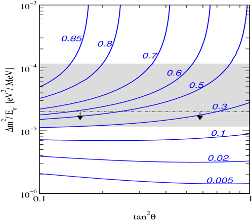
Figure 1: Contours of constant $P_{e1}$. The shaded region is relevant for Borexino, whereas the region below the dash-dotted line is relevant for SK.

The shaded region in Fig. 1 is the region relevant for Borexino, assuming a mass-squared difference in the range $10^{-5}$ eV${}^{2}<\Delta m^{2}<10^{-4}$ eV², whereas for SK the region below the dash-dotted line is most important, due to the higher energy of the ⁸B neutrinos. We can read off from the figure that in most part of the SK region $P_{e1}$ is very small, which means that the sensitivity of SK for $|\mathbf{\Lambda}|$ is limited. In contrast, we expect a much better sensitivity of Borexino because, in a large part of the relevant parameter space in this case, $P_{e1}$ is close to the optimal value of $0.5$.

4 Analysis of solar and reactor neutrino data

In this section we describe briefly our analysis of solar neutrino data and the data which we are using from reactor neutrino experiments. If we neglect the electromagnetic contribution to the small elastic scattering signal in the Sudbury Neutrino Observatory (SNO), the only solar neutrino experiment whose signal will be affected by neutrino TMs is SK. However, the uncertainty in the ⁸B flux leads to correlations between SK and all other experiments. Therefore, also other experiments give some information on TMs and it is important to include them in the analysis [22].

We divide the solar neutrino data into the total rates observed in all experiments and the SK recoil electron spectrum (with free overall normalization). Subsequently we consider the reactor data in combination with the global sample of solar data.

4.1 Solar rates

We include in our fit the event rates measured in the chlorine experiment Homestake [1], the gallium experiments Sage [2], Gallex and GNO [3], the total event rate of SK [4] based on the 1496 days data sample and the result of SNO [5] for the charged current and neutral current solar neutrino rates. For the analysis we use the $\chi^{2}$-function

$$\chi^{2}_{\mathrm{rates}}=\sum_{j,k}(R_{j}-D_{j})(V^{\mathrm{rate}}_{jk})^{-1}(R_{k}-D_{k})\,.$$ (13)

Here the indices $j,k$ run over the 6 solar neutrino rates, $D_{j}$ are the experimental rates and $R_{j}$ are the theoretical predictions, which are calculated as described in Ref. [8], except for the SK experiment, whose rate includes an extra contribution from the electromagnetic scattering, as shown in Ref. [14]. The covariance matrix $V^{\mathrm{rate}}_{jk}$ takes into account the experimental errors and theoretical uncertainties from detection cross sections and SSM predictions of the neutrino fluxes (for details see Refs. [8, 23]).

4.2 The Super-Kamiokande recoil electron spectrum

In this section we consider the shape of the SK recoil electron spectrum. The electromagnetic contribution to the neutrino–electron scattering cross section leads to a different spectrum of the scattered electrons than expected from the SM weak interaction. Therefore, the SK spectral data provide a useful tool to constrain neutrino TMs [24].

We perform a fit to the latest 1496 days SK data presented in Ref. [4] as 44 data points $D_{i}$, using the following $\chi^{2}$-function

$$\chi^{2}_{\mathrm{spect}}=\sum_{i,j=1}^{44}(\alpha R_{i}-D_{i})(V^{\mathrm{spect}}_{ij})^{-1}(\alpha R_{j}-D_{j})\,.$$ (14)

The theoretical prediction $R_{i}$ is calculated as explained in Ref. [14]. The covariance matrix $V^{\mathrm{spect}}_{ij}$ contains statistical and systematic experimental errors, extracted from Ref. [4]. The $\chi^{2}$ is minimized with respect to the normalization factor $\alpha$ in order to isolate only the shape of the spectrum.

4.3 Reactor data

Data from neutrino electron scattering at nuclear reactor experiments can be used to constrain the combination of TMs given in Eq. (8). In fact, these experiments are the most sensitive probe for laboratory searches of neutrino magnetic moment because of the high flux of low-energy antineutrinos emitted by a nuclear reactor and the good experimental control through the on-off reactor comparison. Here we use data from the Rovno nuclear power plant [17], the TEXONO experiment at the Kuo-Sheng Power Plant in Taiwan [18] and from the MUNU experiment at the Bugey reactor [19]. To include this information in our analysis we make the following ansatz for the $\chi^{2}$-function

$$\chi^{2}_{\mathrm{reactor}}(\mu_{\mathrm{R}})=\sum_{i}\left(\frac{N^{i}_{\mathrm{weak}}+N^{i}_{\mathrm{em}}(\mu_{\mathrm{R}})-N^{i}_{\mathrm{obs}}}{\sigma^{i}}\right)^{2}\,.$$ (15)

The sum is over the three experiments. $N^{i}_{\mathrm{obs}}$ is the observed number of events with the one standard deviation error $\sigma^{i}$, $N^{i}_{\mathrm{weak}}$ is the number of events expected in the case of no neutrino TMs (only the standard weak interaction) and $N^{i}_{\mathrm{em}}(\mu_{\mathrm{R}})$ is the number of events due to the electromagnetic scattering of neutrinos with an effective MM $\mu_{\mathrm{R}}$.

5 Bounds on $|\mathbf{\Lambda}|$ from solar and reactor data

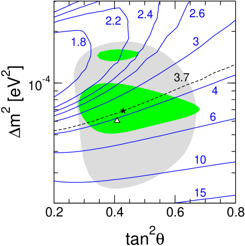
Figure 2: Contours of the 90% C.L. bound on $|\mathbf{\Lambda}|$ in units of $10^{-10}\mu_{B}$ from solar data. The gray (light) shaded region is the 3$\sigma$ LMA-MSW region obtained in the global analysis of solar neutrino data (best fit point marked with a triangle), whereas the green (dark) one corresponds to the 3$\sigma$ region obtained after the inclusion of the KamLAND results in the analysis (best fit point marked with a star), both from Ref. [7]. The dashed line shows the bound obtained at the global best fit point.

First we discuss the bounds on $|\mathbf{\Lambda}|$ from solar data alone. Fixing the oscillation parameters at the current best fit point $\tan^{2}\theta=0.43$, $\Delta m^{2}=6.9\times 10^{-5}$ eV² from the global analysis of solar neutrino data including the KamLAND results [7], we obtain with the Bayesian methods described in Section 3 the 90% C.L. bound

$$|\mathbf{\Lambda}|<3.7\times 10^{-10}\mu_{B}\quad\mbox{(best fit point, solar data)}.$$ (16)

However, such a bound substantially depends on the values of the neutrino oscillation parameters. In Fig. 2 we show contours of the 90% C.L. bound on $|\mathbf{\Lambda}|$ in the $\tan^{2}\theta-\Delta m^{2}$ plane. We find that the bound gets weaker for small values of $\Delta m^{2}$, whereas in the upper left part of the LMA-MSW region a bound of the order $2\times 10^{-10}\mu_{B}$ is obtained.

By combining solar and reactor data we obtain considerably stronger bounds. At the best fit point we get at 90% C.L.

$$|\mathbf{\Lambda}|<1.7\times 10^{-10}\mu_{B}\quad\mbox{(best fit point, solar + reactor data)}.$$ (17)

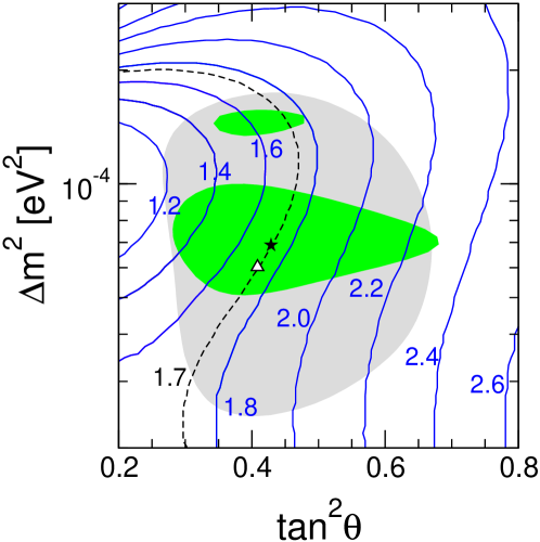
Figure 3: Same as Fig. 2, but here the contours refer to the 90% C.L. bound on $|\mathbf{\Lambda}|$ in units of $10^{-10}\mu_{B}$ from combined solar and reactor data.

In Fig. 3 we show the contours of the bound in the $\tan^{2}\theta-\Delta m^{2}$ plane for the combination of solar and reactor data. By comparing Fig. 2 with Fig. 3 we find that reactor data drastically improve the bound for low $\Delta m^{2}$ values.

In the upper parts of the LMA-MSW region, the solar data alone give already a strong bound on $|\mathbf{\Lambda}|$. This is due to the fact that there the probability $P_{e1}$ relevant in SK is close to the optimal value of 0.5 (see Fig. 1). In this parameter region the combination with reactor data does not improve the bound significantly. In contrast, for low $\Delta m^{2}$ values the probability $P_{e1}$ is very small at the neutrino energies relevant for SK, as seen in Fig. 1. Therefore, solar data give a very weak constraint and only the combination with reactor data improves the bound.

Up to now we have calculated bounds on neutrino TMs for fixed values of the oscillation parameters $\tan^{2}\theta$ and $\Delta m^{2}$ (method I described in Section 3). These results will be especially useful after KamLAND will have determined the oscillation parameters with good accuracy. In the following we change our strategy and minimize the $\chi^{2}$ for each value of $|\mathbf{\Lambda}|$ with respect to $\tan^{2}\theta$ and $\Delta m^{2}$ (method II). This will lead to a bound on $|\mathbf{\Lambda}|$ taking into account the current knowledge concerning the oscillation parameters. To this end we make use of the global solar neutrino data and the latest KamLAND results [16], as described in Ref. [25] in order to obtain the correct $\chi^{2}$ behavior as a function of $\tan^{2}\theta$ and $\Delta m^{2}$. Performing this analysis we obtain the following bounds at 90% C.L.:

$$|\mathbf{\Lambda}|<\left\{\begin{array}[]{l@{\quad}l}4.0\times 10^{-10}\mu_{B}&\mbox{(unconstrained, solar + KamLAND data)}\\ 1.8\times 10^{-10}\mu_{B}&\mbox{(unconstrained, solar + KamLAND + reactor data).}\end{array}\right.$$ (18)

Together with Figs. 2 and 3, the bounds given in Eq. (18) show that current solar neutrino data can be used to constrain all elements of the Majorana neutrino TM matrix. A combination with data from reactor experiments significantly improves the bound on $|\mathbf{\Lambda}|$.

6 Comparison with other works

In this section we compare the quality of our analysis with respect to two previous works doing similar calculations. In particular, we have chosen the first analysis trying to constrain neutrino magnetic moments with solar data, done by Beacom and Vogel [24], and a more recent article presented by Joshipura and Mohanty [22].

In Ref. [24], the SK recoil electron spectrum (825 days) is used to constrain the only component of the Majorana TM matrix present in a 2–neutrino scheme, $\Lambda_{3}$. They obtained $|\Lambda_{3}|$ $\leq$ 1.5$\times$10${}^{-10}\mu_{B}$ at 90% C.L. Using the same assumptions, and just including the SK spectrum shape (1496 days) in the analysis, we get at 90% C.L. $|\Lambda_{3}|$ $\leq$ 1.4$\times$10${}^{-10}\mu_{B}$, which shows the equivalence of the two methods. Taking advantage of the global analysis presented in this work, using all the available information, a better bound is obtained: $|\Lambda_{3}|$ $\leq$ 7.8$\times$10${}^{-11}\mu_{B}$ at 90% C.L.

In the second work [22], the authors assume the general case of three neutrinos and calculate limits on the three elements different from zero of the Majorana TM matrix. To do this, they consider just one component non-zero at a time, and obtain a constraint for each TM separately in the mass basis. As data sample they use only the solar neutrino rates. To compare with their results, we consider just one TM at a time, but we include all the data sample in our analysis. Results are summarized in Tab. 1, where we can see the improvement of the present analysis with respect the two works considered.

Bounds at 90% C.L.
	Beacom & Vogel [24]	Joshipura & Mohanty [22]	present analysis
$|\Lambda_{1}|$ $\leq$	–	4.3$\times$10${}^{-10}\mu_{B}$	1.2$\times$10${}^{-10}\mu_{B}$
$|\Lambda_{2}|$ $\leq$	–	20.5$\times$10${}^{-10}\mu_{B}$	1.0$\times$10${}^{-10}\mu_{B}$
$|\Lambda_{3}|$ $\leq$	1.5$\times$10${}^{-10}\mu_{B}$	3.8$\times$10${}^{-10}\mu_{B}$	7.8$\times$10${}^{-11}\mu_{B}$

Table 1: Comparison of the results from our work and two previous analysis.

Finally, we want to remark that our results are the more general presented up to now, because they are calculated in a 3–neutrino framework, in a basis–independent way and our limits apply to all components of the TM matrix simultaneously. In addition, we have used all the available experimental data, and our bounds are stronger than the obtained in previous calculations.

7 Sensitivity on $|\mathbf{\Lambda}|$ of the Borexino experiment

Here we investigate the sensitivity of the Borexino experiment [26] to neutrino TMs. This experiment is mainly sensitive to the solar ⁷Be neutrino flux, which will be measured by elastic neutrino–electron scattering. Therefore, Borexino is similar to SK, the main difference is the mono-energetic line of the ⁷Be neutrinos, with an energy of 0.862 MeV, which is roughly one order of magnitude smaller than the energies of the ⁸B neutrino flux relevant in SK.

To estimate the sensitivity of Borexino we consider the following $\chi^{2}$-function

$$\chi^{2}_{\mathrm{borexino}}=\sum_{i,j=1}^{N_{\mathrm{bins}}}(N_{i}^{\mathrm{th}}-D_{i})(V^{\mathrm{borex}}_{ij})^{-1}(N_{j}^{\mathrm{th}}-D_{j})\,.$$ (19)

Here $N_{i}^{\mathrm{th}}$ is the theoretical prediction for the number of events in the electron recoil energy bin $i$, given by the sum of events from weak scattering, electromagnetic scattering and background

$$N_{i}^{\mathrm{th}}=N_{i}^{\mathrm{weak}}+N_{i}^{\mathrm{em}}(\mu_{\mathrm{LMA}})+N_{i}^{\mathrm{bg}}\,.$$ (20)

$D_{i}$ is the (hypothetical) observed number of events that, in order to estimate the sensitivity of Borexino for neutrino TMs, we assume generated by neutrinos without TMs

$$D_{i}=N_{i}^{\mathrm{weak}}+N_{i}^{\mathrm{bg}}\,.$$ (21)

Hence, we obtain

$$\chi^{2}_{\mathrm{borexino}}=\sum_{i,j=1}^{N_{\mathrm{bins}}}N_{i}^{\mathrm{em}}\,(V^{\mathrm{borex}}_{ij})^{-1}\,N_{j}^{\mathrm{em}}\,.$$ (22)

The minimum of this $\chi^{2}$ occurs for $\mu_{\mathrm{LMA}}=0$ and is always zero. With this $\chi^{2}$ we calculate a bound on $|\mathbf{\Lambda}|$ at a given C.L. That bound corresponds to the maximum allowed value of $|\mathbf{\Lambda}|$ which cannot be distinguished from $|\mathbf{\Lambda}|=0$, and is therefore a measure for the obtainable sensitivity to $|\mathbf{\Lambda}|$ at Borexino. The definition of the covariance matrix in Eq. (22) and further details about the simulation of Borexino can be found in Ref. [14].

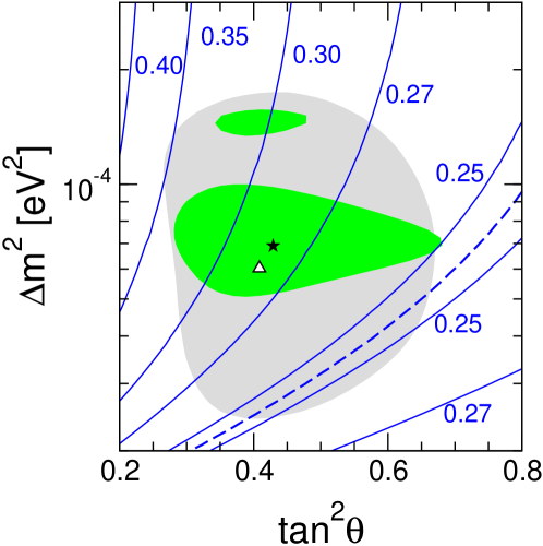
Figure 4: Contours of the 90% C.L. bound on $|\mathbf{\Lambda}|$ after 3 years of Borexino data-taking in units of $10^{-10}\mu_{B}$. The gray (light) shaded region is the allowed LMA-MSW region at 3$\sigma$ obtained in the global solar analysis (best fit point marked with a triangle), and the green (dark) one corresponds to the 3$\sigma$ region obtained including KamLAND in our analysis (best fit point marked with a star), from Ref. [7]. The dashed line corresponds to $P_{e1}=0.5$ for ⁷Be neutrinos, and shows the strongest attainable limit.

Using the statistical method described previously we obtain for the current best fit point $\tan^{2}\theta=0.43$, $\Delta m^{2}=6.9\times 10^{-5}$ eV² the upper bound (sensitivity)

$$|\mathbf{\Lambda}|\leq 0.28\times 10^{-10}\mu_{B}\quad\mbox{at}\quad 90\%\>\mbox{C.L.}$$ (23)

after three years of Borexino data taking. This bound is about one order of magnitude stronger than the bound from existing data, which is partly due to the lower energies observed in Borexino, in comparison with SK. We have checked that a combined analysis of Borexino with existing data (solar and reactor data) does not improve the bound of Eq. (23). In Fig. 4 we show contours of the 90% C.L. bound in the $\tan^{2}\theta-\Delta m^{2}$ plane. The strongest attainable limit is roughly $0.24\times 10^{-10}\mu_{B}$ and, in agreement with the discussion we gave in Sec. 3, it is obtained when $P_{e1}=0.5$, as shown by the dashed line in Fig. 4.

8 Conclusions

In this paper we have presented stringent bounds on electromagnetic Majorana transition moments (TMs). Such TMs can contribute to the elastic neutrino–electron scattering signal in solar neutrino experiments like Super-Kamiokande or the upcoming Borexino experiment, as well as in reactor experiments that detect neutrinos through the neutrino–electron elastic scattering process. Using most recent global solar neutrino data we have performed a fit in terms of the oscillation parameters and the elements of the complex TM matrix $\lambda$ of three active Majorana neutrinos. Taking into account the antisymmetry of the TM matrix, we have shown that solar neutrino data allow to constrain all Majorana TMs simultaneously in a basis independent way, through the intrinsic neutrino property $|\mathbf{\Lambda}|$.

A fit to the global solar neutrino data leads to the bound $|\mathbf{\Lambda}|<4.0\times 10^{-10}\mu_{B}$ at 90% C.L. We have also considered the role of reactor neutrino data on neutrino TMs, shown to be complementary to solar neutrino data. A combined fit of reactor and solar data leads to significantly improved bounds: at 90% C.L. we get $|\mathbf{\Lambda}|<1.8\times 10^{-10}\mu_{B}$. In the near future a precise determination of the oscillation parameters might be possible at the KamLAND experiment, which motivated us to scan the $\tan^{2}\theta-\Delta m^{2}$ plane and to calculate the corresponding bound on $|\mathbf{\Lambda}|$ in each point. These results are shown in Figs. 2 and 3 for solar data and solar + reactor data, respectively. Comparing our results with previous calculations done by other groups we have shown that we have obtained the most general and stringent bounds presented up to this moment.

We have also investigated the potential of the upcoming neutrino–electron scattering solar experiment Borexino to constrain neutrino TMs. Performing a detailed simulation of the experiment we find that it will improve the bound on $|\mathbf{\Lambda}|$ by about one order of magnitude with respect to present bounds.