Lepton Flavour Violation in a Class of Lopsided SO(10) Models

Abstract

A class of predictive SO(10) grand unified theories with highly asymmetric mass matrices, known as lopsided textures, has been developed to accommodate the observed mixing in the neutrino sector. The model class effectively determines the rate for charged lepton flavour violation, and in particular the branching ratio for $\mu\rightarrow e\gamma$, assuming that the supersymmetric GUT breaks directly to the constrained minimal supersymmetric standard model (CMSSM). We find that in light of the combined constraints on the CMSSM parameters from direct searches and from the WMAP satellite observations, the resulting predicted rate for $\mu\rightarrow e\gamma$ in this model class can be within the current experimental bounds for low $\tan\beta$, but that the next generation of $\mu\rightarrow e\gamma$ experiments would effectively rule out this model class if LFV is not detected.

hep-ph/0401132 ALTA-TH-01-04

1 Introduction

Neutrinos have been observed to oscillate between flavour states [1]–[8], which implies neutrino mass and mixing. In addition, the combined observations suggest that both the atmospheric and solar mixing angles are nearly maximal, known as the large angle mixing solution (LMA). Interestingly, the LMA solution implies that the lepton mixing scenario is radically different from the quark sector. From the low energy point of view, we should expect that the neutrino mass inducing dimension 5 operator (HHLL) would be the first observable signal beyond the renormalizable operators that compose the standard model. Furthermore, the smallness of the inferred masses suggests that the mechanism responsible for neutrino mass is distinct from purely electroweak physics, and could naturally arise from physics at a very high scale. The dimension 5 operator can be induced by adding three heavy gauge singlet Majorana fermions (one for each generation) to the standard model. Upon integrating the heavy Majorana fermions out at their associated scale, small neutrino masses are induced after electroweak symmetry breaking. This neutrino mass generating technique is the see-saw mechanism [9].

While the see-saw mechanism is an economical and natural way to understand the smallness of the inferred neutrino masses, there are many possible methods of implementing it, and therefore detailed neutrino observations can be used to constrain GUT models. Perhaps the most elegant GUT uses the grand unifying group SO(10) in four spacetime dimensions. The spinor representation of SO(10) is 16 dimensional, which accommodates all the helicity states of one fermion family plus an extra singlet degree of freedom for a Majorana neutrino. The generations are simply three copies of the spinor representation. Since GUTs relate quark and lepton masses and mixings, it is perplexing from a model building perspective as to why lepton mixing is so different from that in the quark sector. More specifically, it is of interest to understand why $|U_{\mu 3}|$ of the MNS matrix is so much larger than $|V_{cb}|$ of the CKM matrix. Over the last few years a number of models have been developed to address this difference [10]–[20]. Recently, a particularly interesting and highly successful class of supersymmetric SO(10) GUTs has emerged that makes use of asymmetric mass matrices known as lopsided textures [10, 11, 12]. In these models, the charged lepton sector is responsible for the large atmospheric mixing angle while the Majorana singlet neutrino matrix has a simple form that results in the large solar mixing angle. Throughout this paper we will refer to these models as the AB model class [10].

After GUT breaking, these models reduce to the R-parity conserving minimal supersymmetric standard model (MSSM) with specific model dependent relationships amongst the Yukawa couplings. In addition to the constraints already provided by the neutrino physics (and the demand that these models reproduce all the low energy physics of the standard model), the WMAP satellite observations [21] provide strong constraints on the available supersymmetric parameter space if the lightest supersymmetic particle (LSP) is assumed to compose the dark matter [22, 23, 24]. Assuming the constraints on the CMSSM from the WMAP data, the definite flavour structure of the AB models will result in specific soft supersymmetry breaking parameters. Therefore, the AB model class gives well defined predictions for lepton flavour violation and in particular $\mu\rightarrow e\gamma$. It is of considerable interest to determine how the lepton flavour changing neutral current bounds restrict the CMSSM parameters for the AB model class in light of the WMAP data.

We organize this paper as follows. In section 2 we outline the essential details of the AB models, the supersymmetric parameter space, and the calculation for $\mu\rightarrow e\gamma$. We consider $\mu\rightarrow e\gamma$ since at the present time, with the current bound [25] of $\mathrm{BR}(\mu\rightarrow e\gamma)<1.2\times 10^{-11}$, this process gives the strongest constraints on lepton flavour violation in the class of models that we discuss. Furthermore, the MEG experiment at PSI [26] expects to improve on this bound with the expected sensitivity of $\mathrm{BR}(\mu\rightarrow e\gamma)\lesssim 5\times 10^{-14}$. This experiment will provide stringent limits on models with charged lepton flavour violation. In section 3 we display our numerical results with the combined constraints from $\mu\rightarrow e\gamma$ and the WMAP satellite observations, and in section 4 we present our conclusions. The appendix provides further calculational details.

2 The AB Model Definition

The AB model class is based on an SO(10) GUT with a U(1)$\times$Z₂$\times$Z₂ flavour symmetry and uses a minimum set of Higgs fields to solve the doublet-triplet splitting problem [10, 11, 12]. The interesting feature of these models is the use of a lopsided texture. The approximate form of the charged lepton and the down quark mass matrix in these models is given by

$$\begin{array}[]{cc}\mathbf{Y}_{\mathrm{E}}\sim\left(\begin{array}[]{ccc}0&0&0\\ 0&0&\epsilon\\ 0&\sigma&1\end{array}\right),&\mathbf{Y}_{\mathrm{D}}\sim\left(\begin{array}[]{ccc}0&0&0\\ 0&0&\sigma\\ 0&\epsilon&1\end{array}\right).\end{array}$$ (1)

where $\sigma\sim 1$ and $\epsilon\ll 1$. As pointed out by the authors of [10], this asymmetric structure naturally occurs within a minimal SU(5) GUT where the Yukawa interaction for the down quarks and leptons is of the form $\lambda_{ij}{\bf\bar{5}}_{i}{\bf 10}_{j}{\bf 5_{H}}$ (${\bf 5_{H}}$ denotes the Higgs scalars). In an SU(5) GUT, the left-handed leptons and the charge conjugate right-handed down quarks belong to the ${\bf\bar{5}}$ while the ${\bf 10}$ contains the charge conjugate right-handed leptons and the left-handed down quarks. Therefore the lepton and down quark mass matrices are related to each other by a left-right transpose. Since SU(5) is a subgroup of SO(10), this feature is retained in an SO(10) GUT. This lopsided texture has the ability to explain why $|U_{\mu 3}|>>|V_{cb}|$. Making use of this observation, the AB models contain the Dirac matrices ${\bf U},{\bf N},{\bf D},{\bf L}$ for the up-like quarks, Dirac neutrino interaction, down-like quarks, and the leptons respectively [12],

$$\begin{array}[]{cc}{\bf U}=\left(\begin{array}[]{ccc}\eta&0&0\\ 0&0&\epsilon/3\\ 0&-\epsilon/3&1\end{array}\right)M_{U},&{\bf N}=\left(\begin{array}[]{ccc}\eta&0&0\\ 0&0&-\epsilon\\ 0&\epsilon&1\end{array}\right)M_{U},\end{array}$$ (2)

$$\begin{array}[]{cc}{\bf D}=\left(\begin{array}[]{ccc}0&\delta&\delta^{\prime}e^{i\phi}\\ \delta&0&\sigma+\epsilon/3\\ \delta^{\prime}e^{i\phi}&-\epsilon/3&1\end{array}\right)M_{D},&{\bf L}=\left(\begin{array}[]{ccc}0&\delta&\delta^{\prime}e^{i\phi}\\ \delta&0&-\epsilon\\ \delta^{\prime}e^{i\phi}&\sigma+\epsilon&1\end{array}\right)M_{D}.\end{array}$$ (3)

where

$$\begin{array}[]{rclcrcl}M_{U}&\approx&113\;\mathrm{GeV},&&M_{D}&\approx&1\;\mathrm{GeV},\\ \sigma&=&1.78,&&\epsilon&=&0.145,\\ \delta&=&8.6\times 10^{-3},&&\delta^{\prime}&=&7.9\times 10^{-3},\\ \phi&=&126^{\circ},&&\eta&=&8\times 10^{-6}.\end{array}$$ (4)

Dimensionless Yukawa couplings $\mathbf{Y}_{\mathrm{U}},\mathbf{Y}_{\mathrm{N}},\mathbf{Y}_{\mathrm{D}}$, and $\mathbf{Y}_{\mathrm{E}}$ can be extracted from the Dirac matrices. The given values of $M_{D}$ and $M_{U}$ best fit the low energy data with $\tan\beta\approx 5$. It should be noted that larger values of $\tan\beta$ are easily accommodated by altering the values of $M_{U}$ and $M_{D}$ while retaining accurate fits to the low energy data after renormalization group running. The lopsided texture of the AB model class nicely fits the large atmospheric mixing angle; however, in order to obtain the large solar mixing angle a specific hierarchical form of the heavy Majorana singlet neutrino matrix needs to be chosen [11, 12], namely,

$${\mathbf{M}_{\mathrm{N}}}=\left(\begin{array}[]{ccc}b^{2}\eta^{2}&-b\epsilon\eta&a\eta\\ -b\epsilon\eta&\epsilon^{2}&-\epsilon\\ a\eta&-\epsilon&1\end{array}\right)\Lambda_{\mathrm{N}}.$$ (5)

where the parameters $\epsilon$ and $\eta$ are as defined in equation (4). The parameters $a$ and $b$ are of order $1$ and $\Lambda_{\mathrm{N}}\sim 2\times 10^{14}$ GeV. Since the Majorana singlet neutrino matrix is not related to the Dirac Yukawa structure, it is not surprising that this matrix should take on a form independent from the rest of the model. Once these choices have been made, the AB model class is highly predictive and accurately fits all the low energy standard model physics and the neutrino mixing observations.

It should be emphasized that all these relations are defined at the GUT scale and are therefore subject to renormalization group running [9]. If we conservatively assume that the GUT symmetry breaks directly to the standard model gauge symmetries, SU(3)$\times$SU(2)$\times$U(1), and that supersymmetry is broken super-gravitionally through a hidden sector in a flavour independent manner, the AB model class will give well defined predictions for charged lepton flavour violation. There may also be significant contributions to the off-diagonal elements from renormalization group running between the GUT and gravity scales [28, 29]. Since the particulars of GUT and supersymmetry breaking – as well as the possibility of new physics above the GUT scale – can have model dependent effects on the branching ratio for $\mu\rightarrow e\gamma$, we do not consider an interval of running between the GUT and gravity scales.

The specific model predictions for the Dirac Yukawa couplings and the form of the Majorana singlet neutrino matrix will feed into the soft supersymmetry breaking slepton mass terms through renormalization group running, generating off diagonal elements that will contribute to flavour changing neutral currents [27]. The amount of flavour violation contained in the AB model class can be examined through the branching ratio of the process $\mu\rightarrow e\gamma$.

3 Numerical Results for $\mu\rightarrow e\gamma$

After GUT and supersymmetry breaking, we have the constrained minimal supersymmetric standard model (CMSSM) with heavy gauge singlet neutrinos to make use of the see-saw mechanism. The leptonic part of the superpotential is

$$W=\epsilon_{\alpha\beta}H_{\mathrm{d}}^{\alpha}{\mathbf{E}}\mathbf{Y}_{\mathrm{E}}{\mathbf{L}}^{\beta}+\epsilon_{\alpha\beta}H_{\mathrm{u}}^{\alpha}{\mathbf{N}}\mathbf{Y}_{\mathrm{N}}{\mathbf{L}}^{\beta}+\frac{1}{2}{\mathbf{N}}\mathbf{M}_{\mathrm{N}}{\mathbf{N}}$$ (6)

where $\mathbf{Y}_{\mathrm{E}}$, $\mathbf{Y}_{\mathrm{N}}$ are Yukawa matrices, and $\mathbf{M}_{\mathrm{N}}$ is the singlet Majorana neutrino mass matrix. The totally antisymmetric symbol is defined $\epsilon_{12}=+1$. We explain our notation in detail in the appendix. On integrating out the heavy singlet neutrinos, equation (6) reduces to

$$W=\epsilon_{\alpha\beta}H_{\mathrm{d}}^{\alpha}\mathbf{E}\mathbf{Y}_{\mathrm{E}}\mathbf{L}^{\beta}-\frac{1}{2}\mathbf{\nu}^{\mathrm{T}}\mathbf{m}_{\nu}\mathbf{\nu}$$ (7)

where

$$\mathbf{m}_{\nu}=\frac{v^{2}}{2}\mathbf{Y}_{\mathrm{N}}^{\mathrm{T}}\mathbf{M}_{\mathrm{N}}^{-1}\mathbf{Y}_{\mathrm{N}}\sin^{2}\beta$$ (8)

is the see-saw induced light neutrino mass matrix. The coefficients $\beta$ and $v$ are defined in terms of Higgs fields expectation values by

$$\frac{v^{2}}{2}=\left<H_{\mathrm{d}}^{0}\right>^{2}+\left<H_{\mathrm{u}}^{0}\right>^{2}=\left(174\;\mathrm{GeV}\right)^{2},\quad\quad\tan\beta=\frac{\left<H_{\mathrm{u}}^{0}\right>}{\left<H_{\mathrm{d}}^{0}\right>}.$$ (9)

The neutrino mass matrix, equation (8), is in general not diagonal and this is the source of lepton flavour violating interactions.

We assume that supersymmetry is broken softly in that breaking occurs through operators of mass dimension 2 and 3. The soft supersymmetry breaking Lagrangian relevant to LFV studies is

$$\mathcal{L}_{\mathrm{breaking}} = -\delta_{\alpha\beta}\tilde{\mathbf{L}}^{\alpha\dagger}\mathbf{m}^{2}_{\tilde{\mathrm{L}}}\tilde{\mathbf{L}}^{\beta}-\tilde{\mathbf{E}}\mathbf{m}^{2}_{\tilde{\mathrm{E}}}\tilde{\mathbf{E}}^{\dagger}-\tilde{\mathbf{N}}\mathbf{m}^{2}_{\tilde{\mathrm{N}}}\tilde{\mathbf{N}}^{\dagger}$$ (10)

$$-m^{2}_{\mathrm{H_{d}}}\delta_{\alpha\beta}H_{\mathrm{d}}^{\alpha*}H_{\mathrm{d}}^{\beta}-m^{2}_{\mathrm{H_{u}}}\delta_{\alpha\beta}H_{\mathrm{u}}^{\alpha*}H_{\mathrm{u}}^{\beta}$$

$$\left(-B\epsilon_{\alpha\beta}H_{\mathrm{d}}^{\alpha}H_{\mathrm{u}}^{\beta}-\frac{1}{2}\tilde{\mathbf{N}}\mathbf{B}_{\tilde{\mathrm{N}}}\tilde{\mathbf{N}}\;+\;\mathrm{c.\;c.}\right)$$

$$\left(-\epsilon_{\alpha\beta}H_{\mathrm{d}}^{\alpha}\tilde{\mathbf{E}}\mathbf{A}_{\mathrm{E}}\tilde{\mathbf{L}}^{\beta}-\epsilon_{\alpha\beta}H_{\mathrm{u}}^{\alpha}\tilde{\mathbf{N}}\mathbf{A}_{\mathrm{N}}\tilde{\mathbf{L}}^{\beta}\;+\;\mathrm{c.\;c.}\right)$$

$$\left(-\frac{1}{2}M_{1}\tilde{B}\tilde{B}-\frac{1}{2}M_{2}\tilde{W}^{a}\tilde{W}^{a}\;+\;\mathrm{c.\;c.}\right)$$

(see the appendix for the notational details). The CMSSM assumes universal soft supersymmetry breaking parameters at the supersymmetry breaking scale, which we take to be of order the GUT scale, leading to the following GUT relations:

$$\mathbf{m}^{2}_{\tilde{\mathrm{L}}}=\mathbf{m}^{2}_{\tilde{\mathrm{E}}}=\mathbf{m}^{2}_{\tilde{\mathrm{N}}}=m_{0}^{2}\cdot\mathbf{I},$$ (11)

$$m^{2}_{\mathrm{H_{d}}}=m^{2}_{\mathrm{H_{u}}}=m_{0}^{2},$$ (12)

$$\mathbf{A}_{\mathrm{E}}=\mathbf{A}_{\mathrm{N}}=0,$$ (13)

$$M_{1}=M_{2}=m_{1/2}$$ (14)

where $m_{0}$ and $m_{1/2}$ denote the universal scalar mass and the universal gaugino mass respectively ($\mathbf{I}$ is the 3$\times$3 unit matrix). We conservatively assume that the trilinear terms $\mathbf{A}_{\mathrm{E}}$ and $\mathbf{A}_{\mathrm{N}}$ vanish at the supersymmetry breaking scale.

We run the parameters of the CMSSM using the renormalization group equations (see appendix) working in a basis where the Majorana neutrino singlet matrix is diagonal, integrating out each heavy neutrino singlet at its associated scale. After integrating down to the electroweak scale, we rotate the Yukawa couplings to the mass eigenbasis. In order to understand the origin of flavour violation in this model class, we first give a qualitative estimate. The leading log approximation of the off-diagonal slepton mass term is given by

$$\left(\Delta\mathbf{m}^{2}_{\tilde{\mathrm{L}}}\right)_{ij}\approx-\frac{3}{8\pi^{2}}m_{0}^{2}({\bf Y_{\nu}}^{\dagger}{\bf Y_{\nu}})\ln\left(\frac{M_{\mathrm{GUT}}}{{\Lambda_{\mathrm{N}}}}\right),$$ (15)

(assuming that the trilinears vanish at the GUT scale), and using this approximation together with mass insertion techniques [29, 30], the branching ratio for $\mu\rightarrow e\gamma$ is

$$\mathrm{BR}(\mu\rightarrow e\gamma) \sim \frac{\alpha^{3}}{G_{\mathrm{F}}^{2}}\frac{\left(\left(\mathbf{m}^{2}_{\tilde{\mathrm{L}}}\right)_{12}\right)^{2}}{m_{\mathrm{s}}^{8}}\tan^{2}\beta$$ (16)

$$\approx \frac{\alpha^{3}}{G_{\mathrm{F}}^{2}m_{\mathrm{s}}^{8}}\left|\frac{3}{8\pi^{2}}m_{0}^{2}\ln\frac{M_{\mathrm{GUT}}}{\Lambda_{\mathrm{N}}}\right|^{2}\left|\left({\bf Y_{\nu}}^{\dagger}{\bf Y_{\nu}}\right)_{12}\right|^{2}\tan^{2}\beta$$

where $m_{s}$ is a typical sparticle mass. We see that since the flavour structure of the AB model class is specified so precisely, the branching ratio for $\mu\rightarrow e\gamma$ is well determined. In our calculation of the decay rate, we use the full one-loop expressions derived from the diagrams in figure 1 (see the appendix for more details).

The WMAP satellite observations [21] combined with constraints from $b\rightarrow s\gamma$ and LEP direct searches [31] strongly limit the available CMSSM parameter space if the LSP composes the dark matter [22, 23, 24]. In addition to these constraints, realistic supersymmetric GUT models must also survive LFV bounds, such as the limit on $\mu\rightarrow e\gamma$. In particular, using all of the available bounds, both cosmological and laboratory, we can further restrict the AB model class.

Figure 1: Feynman diagrams contributing to $\mu\rightarrow e\gamma$.

In figure 2, we show contours of the branching ratio $\mu\rightarrow e\gamma$ in the $m_{1/2}$-$m_{0}$ plane for a variety of $\tan\beta$ with the $\mu$ parameter both positive and negative. The parameters of the AB model class have been chosen such that all the low energy predictions fit the standard model data, and we have chosen $a=1$ and $b=2$ for the Majorana singlet neutrino mass matrix given in equation (5). As indicated in [12], there are a number of possible model choices for the Majorana singlet parameters $a$ and $b$ that are consistent with the LMA solution. However, we find that the rate for $\mu\rightarrow e\gamma$ is largely unaffected by the allowed range [12] for these parameters.

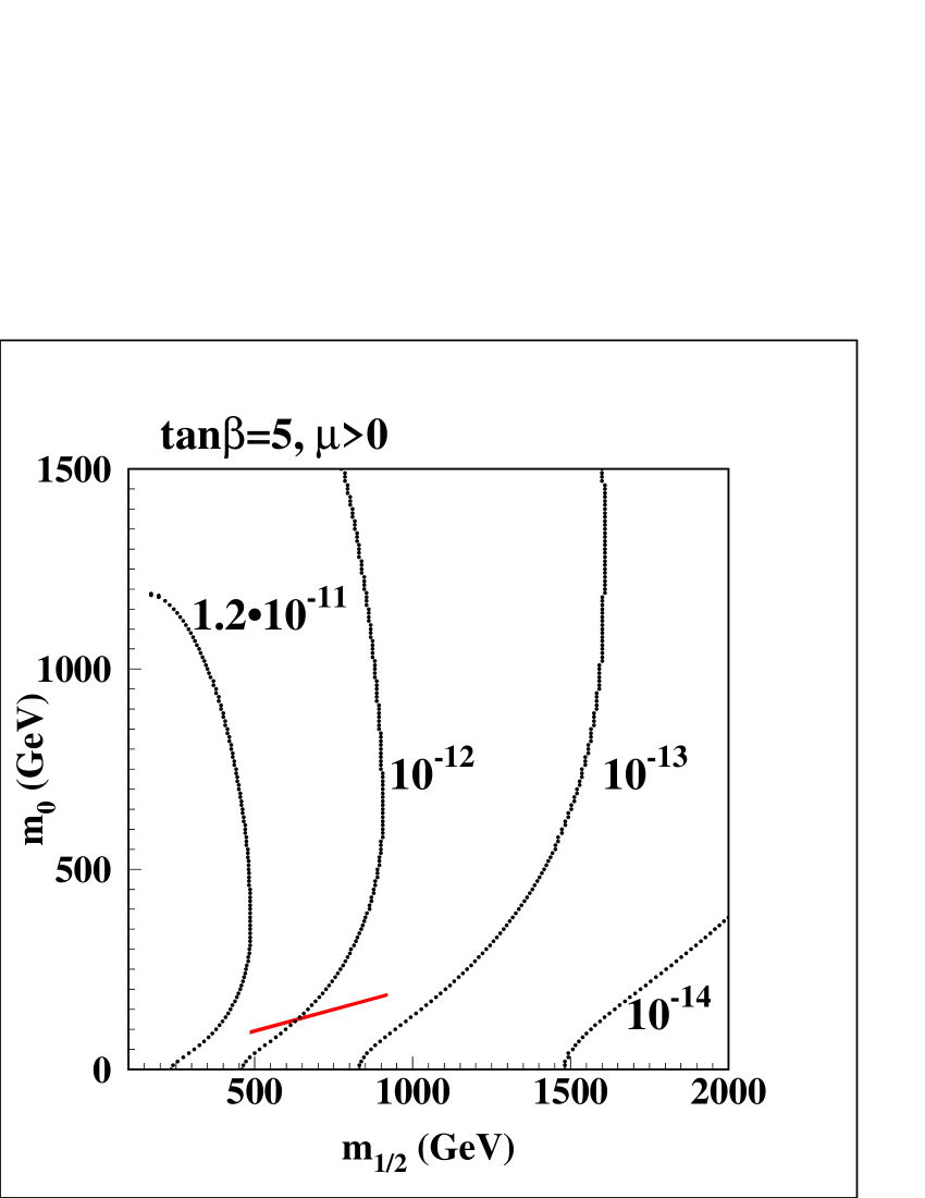
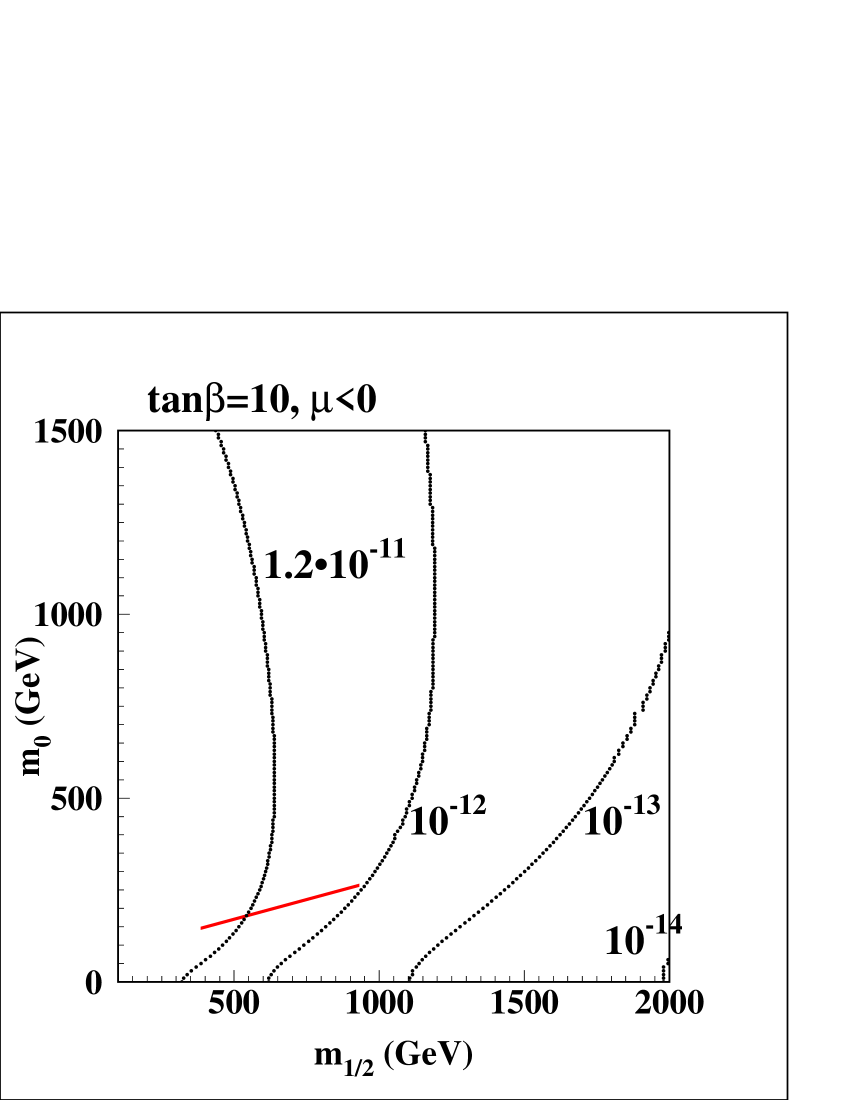
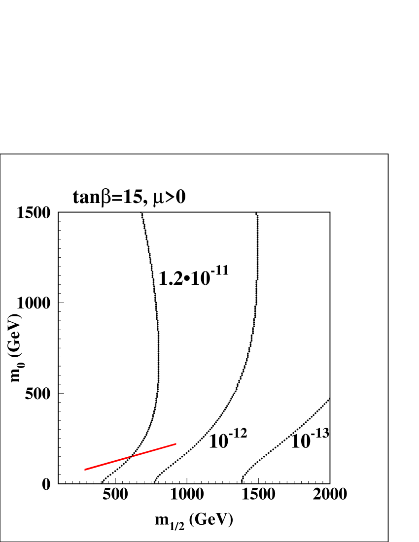
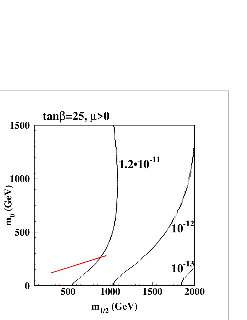
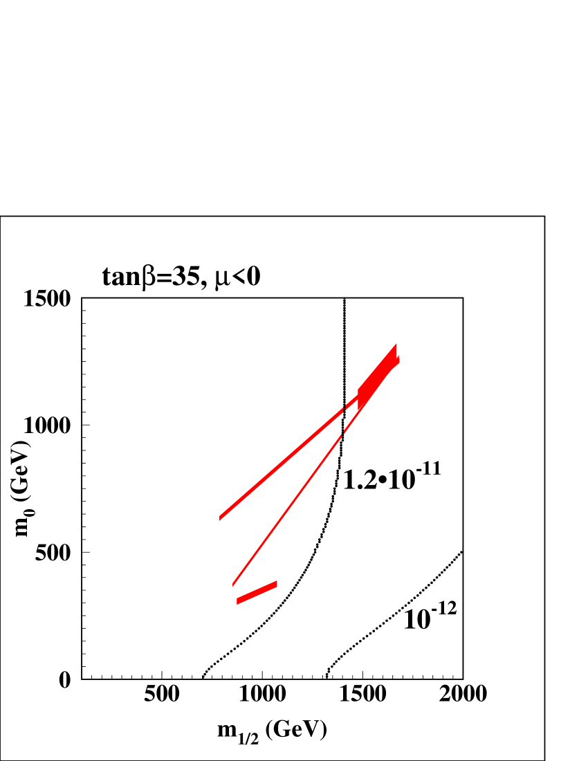
Figure 2: Contour Plots of $\mathrm{BR}(\mu\rightarrow e\gamma)$ in the $m_{0}-m_{1/2}$ plane: Panels (a),(c),(d), and (f) show the contours of the branching ratio for $\tan\beta=5,15,25,50$ respectively with $\mu>0$. Panels (b) and (e) show the contours with $\tan\beta=10,35$ respectively with $\mu<0$. In all cases the shaded region corresponds to the approximate combined WMAP and laboratory constraints.

Panel (a) demonstrates the lepton flavour bounds for $\tan\beta=5$ with $\mu>0$ . The small line-like shaded area in the lower part of the panel is the allowed region from the combined WMAP and laboratory limits. The remaining panels show that the contours of constant branching ratio migrate to the right of the plots (i.e. to high values of $m_{1/2}$ and $m_{0}$) as $\tan\beta$ is increased. In each case we overlay the approximate WMAP and laboratory constraint bounds represented by a shaded region [22]. The choice for the sign of $\mu$ is indicated in each panel. As $\tan\beta$ is pushed up, larger portions of the parameter space become excluded. This is an expected feature since the branching ratio is proportional to $\tan^{2}\beta$. Notice that by $\tan\beta\sim 25$, $\mu>0$, the branching ratio allowed contours no longer have a significant overlap with the WMAP region. As a result, we find that the AB model class is consistent with the current experimental bound on $\mu\rightarrow e\gamma$ for low $\tan\beta$ (i.e. $\tan\beta\lesssim 20$) for $\mu>0$. For completeness, in panels (b) and (e), we show two cases where $\mu<0$. The branching ratio of $\mu\rightarrow e\gamma$ is largely insensitive to the sign of $\mu$, however the WMAP region is moderately affected [23]. A small part of the allowed WMAP region is currently permitted for larger $\tan\beta$ (i.e. $\sim 35$) as indicated in panel (e). The upcoming limits [26] that MEG will establish, $\mathrm{BR}(\mu\rightarrow e\gamma)\lesssim 5\times 10^{-14}$, will effectively rule out this model class if LFV is not seen. Interestingly, if LFV is seen at MEG, this model will suggest that $\tan\beta$ is low based on flavour bounds alone.

4 Conclusions

The AB model class [10, 11, 12], based on a U(1)$\times$Z₂$\times$Z₂ flavour symmetry, is a highly successful and predictive GUT scenario. This model class has the ability to accommodate all the observed neutrino phenomena and reproduce the low energy physics of the standard model. If it is assumed that supersymmetry is broken via mSUGRA and that the GUT breaks directly to the CMSSM, the AB model class is highly restrictive and hence allows for a precise determination for the rate of charged lepton flavour violation. In particular, we examined the process $\mu\rightarrow e\gamma$, since at the present time this flavour violating muon decay channel gives the strongest constraints on flavour changing neutral currents in the lepton sector.

As the WMAP satellite data [21] and laboratory direct searches [31] have already severely restricted the available CMSSM parameter space, the $\mu\rightarrow e\gamma$ flavour bounds allow a strong test of the AB model class. We find that given the current bounds [25] on $\mu\rightarrow e\gamma$, $\mathrm{BR}(\mu\rightarrow e\gamma)<1.2\times 10^{-11}$, the AB model class favours low $\tan\beta$ (i.e. $\lesssim 20$) with $\mu>0$, however, there is a small region that is not excluded for $\tan\beta\lesssim 35$ with the sign of $\mu$ negative. If MEG at PSI [26] does not detect a positive LFV signal, $\mathrm{BR}(\mu\rightarrow e\gamma)\lesssim 5\times 10^{-14}$, the AB model class will be effectively ruled out, given our conservative assumptions concerning GUT and supersymmetry breaking. It remains an open question as to whether or not other supersymmetry and/or GUT breaking schemes within the AB model class will be able to avoid these flavour violating bounds.

5 Acknowledgements

We would like to thank Bruce A. Campbell for helpful discussions and comments. DM acknowledges the support of the Natural Sciences and Engineering Research Council of Canada and EJ the support of the Alberta Ingenuity Fund.

6 Appendix

In this section we wish to clarify some of the calculational details. We carefully establish our notation and conventions. Also, we include the full one loop amplitude for the rate $\mu\rightarrow e\gamma$ that we used in our calculations. Formulas similar to those given in subsections 6.2-6.6 can be found in [30].

We express the supersymmetric Lagrangian using the 2-component Weyl formalism. $\mathbf{L}^{\alpha}=\left(L^{\alpha}_{1},L^{\alpha}_{2},L^{\alpha}_{3}\right)^{\mathrm{T}}$ denotes a column vector in generation space containing the SU(2) doublet lepton chiral superfields; 1,2,3 are generation labels, and $\alpha=1,2$ are the SU(2) indices. $\mathbf{E}=\left(E_{1},E_{2},E_{3}\right)$ denotes a row vector in generation space containing SU(2) singlet charged lepton superfields. The gauge singlet neutrino chiral superfields are denoted by $\mathbf{N}=\left(N_{1},N_{2},N_{3}\right)$. Similarly, for the quark superfields: $\mathbf{Q}^{\alpha}=\left(Q^{\alpha}_{1},Q^{\alpha}_{2},Q^{\alpha}_{3}\right)^{\mathrm{T}}$ denotes the SU(2) doublet, $\mathbf{Q}^{1}=\mathbf{u}=\left(u_{1},u_{2},u_{3}\right)^{\mathrm{T}}$, $\mathbf{Q}^{2}=\mathbf{d}=\left(d_{1},d_{2},d_{3}\right)^{\mathrm{T}}$; and the SU(2) singlet quark superfields are $\mathbf{U}=\left(U_{1},U_{2},U_{3}\right)$, $\mathbf{D}=\left(D_{1},D_{2},D_{3}\right)$. $H_{\mathrm{d}}^{\alpha}$, $H_{\mathrm{u}}^{\alpha}$ are the SU(2) Higgs doublet superfields of opposite hypercharge with the standard components: $H_{\mathrm{d}}^{\alpha=1}=H_{\mathrm{d}}^{0}$, $H_{\mathrm{d}}^{\alpha=2}=H_{\mathrm{d}}^{-}$, $H_{\mathrm{u}}^{\alpha=1}=H_{\mathrm{u}}^{+}$, $H_{\mathrm{u}}^{\alpha=2}=H_{\mathrm{u}}^{0}$. The corresponding scalar components of the superfields are written respectively as $\tilde{\mathbf{L}}^{\alpha}$, $\tilde{\mathbf{L}}^{1}=\tilde{\nu}$, $\tilde{\mathbf{L}}^{2}=\tilde{\mathbf{e}}$; $\tilde{\mathbf{E}}$; $\tilde{\mathbf{N}}$; $\tilde{\mathbf{Q}}^{\alpha}$, $\tilde{\mathbf{Q}}^{1}=\tilde{\mathbf{u}}$, $\tilde{\mathbf{Q}}^{2}=\tilde{\mathbf{d}}$; $\tilde{\mathbf{D}}$; $\tilde{\mathbf{U}}$; (all are vectors in generation space). The fermionic components of the Higgs superfield, the Higgsinos, are denoted as $\tilde{H}^{\alpha}_{\mathrm{d}}$, $\tilde{H}^{\alpha}_{\mathrm{u}}$. The superpotential $W$ is given by

$$W= \epsilon_{\alpha\beta}H_{\mathrm{d}}^{\alpha}\mathbf{E}\mathbf{Y}_{\mathrm{E}}\mathbf{L}^{\beta}+\epsilon_{\alpha\beta}H_{\mathrm{u}}^{\alpha}\mathbf{N}\mathbf{Y}_{\mathrm{N}}\mathbf{L}^{\beta}+\frac{1}{2}\mathbf{N}\mathbf{M}_{\mathrm{N}}\mathbf{N}$$ (17)

$$+ \epsilon_{\alpha\beta}H_{\mathrm{d}}^{\alpha}\mathbf{D}\mathbf{Y}_{\mathrm{D}}\mathbf{Q}^{\beta}+\epsilon_{\alpha\beta}H_{\mathrm{u}}^{\alpha}\mathbf{U}\mathbf{Y}_{\mathrm{U}}\mathbf{Q}^{\beta}$$

$$+ \mu\epsilon_{\alpha\beta}H_{\mathrm{d}}^{\alpha}H_{\mathrm{u}}^{\beta}$$

where $\mathbf{Y}_{\mathrm{E}}$, $\mathbf{Y}_{\mathrm{N}}$, $\mathbf{Y}_{\mathrm{D}}$, $\mathbf{Y}_{\mathrm{U}}$ are Yukawa matrices $\mathbf{M}_{\mathrm{N}}$ is the singlet Majorana neutrino mass matrix, $\mu$ is the Higgs parameter that breaks the U(1) Pecci-Quinn symmetry, and the totally antisymmetric symbol is defined $\epsilon_{12}=+1$. The soft supersymmetry breaking Lagrangian is

$$\mathcal{L}_{\mathrm{breaking}} = -\delta_{\alpha\beta}\tilde{\mathbf{L}}^{\alpha\dagger}\mathbf{m}^{2}_{\tilde{\mathrm{L}}}\tilde{\mathbf{L}}^{\beta}-\tilde{\mathbf{E}}\mathbf{m}^{2}_{\tilde{\mathrm{E}}}\tilde{\mathbf{E}}^{\dagger}-\tilde{\mathbf{N}}\mathbf{m}^{2}_{\tilde{\mathrm{N}}}\tilde{\mathbf{N}}^{\dagger}$$ (18)

$$-\delta_{\alpha\beta}\tilde{\mathbf{Q}}^{\alpha\dagger}\mathbf{m}^{2}_{\tilde{\mathrm{Q}}}\tilde{\mathbf{Q}}^{\beta}-\tilde{\mathbf{D}}\mathbf{m}^{2}_{\tilde{\mathrm{D}}}\tilde{\mathbf{D}}^{\dagger}-\tilde{\mathbf{U}}\mathbf{m}^{2}_{\tilde{\mathrm{U}}}\tilde{\mathbf{U}}^{\dagger}$$

$$-m^{2}_{\mathrm{H_{d}}}\delta_{\alpha\beta}H_{\mathrm{d}}^{\alpha*}H_{\mathrm{d}}^{\beta}-m^{2}_{\mathrm{H_{u}}}\delta_{\alpha\beta}H_{\mathrm{u}}^{\alpha*}H_{\mathrm{u}}^{\beta}$$

$$\left(-b\epsilon_{\alpha\beta}H_{\mathrm{d}}^{\alpha}H_{\mathrm{u}}^{\beta}-\frac{1}{2}\tilde{\mathbf{N}}\mathbf{B}_{\mathrm{\tilde{N}}}\tilde{\mathbf{N}}\;+\;\mathrm{c.\;c.}\right)$$

$$\left(-\epsilon_{\alpha\beta}H_{\mathrm{d}}^{\alpha}\tilde{\mathbf{E}}\mathbf{A}_{\mathrm{E}}\tilde{\mathbf{L}}^{\beta}-\epsilon_{\alpha\beta}H_{\mathrm{u}}^{\alpha}\tilde{\mathbf{N}}\mathbf{A}_{\mathrm{N}}\tilde{\mathbf{L}}^{\beta}\;+\;\mathrm{c.\;c.}\right)$$

$$\left(-\epsilon_{\alpha\beta}H_{\mathrm{d}}^{\alpha}\tilde{\mathbf{D}}\mathbf{A}_{\mathrm{D}}\tilde{\mathbf{Q}}^{\beta}-\epsilon_{\alpha\beta}H_{\mathrm{u}}^{\alpha}\tilde{\mathbf{U}}\mathbf{A}_{\mathrm{U}}\tilde{\mathbf{Q}}^{\beta}\;+\;\mathrm{c.\;c.}\right)$$

$$\left(-\frac{1}{2}M_{1}\tilde{B}\tilde{B}-\frac{1}{2}M_{2}\tilde{W}^{a}\tilde{W}^{a}-\frac{1}{2}M_{3}\tilde{G}^{b}\tilde{G}^{b}\;+\;\mathrm{c.\;c.}\right)$$

where $\tilde{B}$ denotes electroweak U(1) gaugino field; $\tilde{W}^{a}$, $a=1,2,3$, denote electroweak SU(2) gaugino fields; $\tilde{G}^{b}$, $b=1,...,8$, denote strong interaction, SU(3), gaugino fields; $\mathbf{m}^{2}_{\tilde{\mathrm{L}}}$, $\mathbf{m}^{2}_{\tilde{\mathrm{E}}}$, $\mathbf{m}^{2}_{\tilde{\mathrm{N}}}$, $\mathbf{m}^{2}_{\tilde{\mathrm{Q}}}$, $\mathbf{m}^{2}_{\tilde{\mathrm{D}}}$, $\mathbf{m}^{2}_{\tilde{\mathrm{U}}}$, $\mathbf{B}_{\nu}$, $\mathbf{A}_{\mathrm{E}}$, $\mathbf{A}_{\mathrm{N}}$, $\mathbf{A}_{\mathrm{D}}$, $\mathbf{A}_{\mathrm{U}}$, $m^{2}_{\mathrm{H_{d}}}$, $m^{2}_{\mathrm{H_{u}}}$, $b$, $M_{1}$, $M_{2}$, $M_{3}$ are the supersymmetry breaking parameters, and at the GUT scale:

$$\mathbf{m}^{2}_{\tilde{\mathrm{L}}}=\mathbf{m}^{2}_{\tilde{\mathrm{E}}}=\mathbf{m}^{2}_{\tilde{\mathrm{N}}}=\mathbf{m}^{2}_{\tilde{\mathrm{Q}}}=\mathbf{m}^{2}_{\tilde{\mathrm{D}}}=\mathbf{m}^{2}_{\tilde{\mathrm{U}}}=m_{0}^{2}\cdot\mathbf{I},$$ (19)

$$m^{2}_{\mathrm{H_{d}}}=m^{2}_{\mathrm{H_{u}}}=m_{0}^{2},$$ (20)

$$\mathbf{A}_{\mathrm{E}}=\mathbf{A}_{\mathrm{N}}=\mathbf{A}_{\mathrm{D}}=\mathbf{A}_{\mathrm{U}}=0,$$ (21)

$$M_{1}=M_{2}=M_{3}=m_{1/2}$$ (22)

where $m_{0}$ and $m_{1/2}$ denote the universal scalar mass and the universal gaugino mass respectively ($\mathbf{I}$ is the 3$\times$3 unit matrix). After running the CMSSM RGEs (see subsection 6.6), we rotate all the Yukawa couplings to a diagonal basis, and in particular the lepton sector,

$$\mathbf{Y}_{\mathrm{E}}\quad \rightarrow \quad\mathbf{U}_{\mathrm{E}}^{*}\mathbf{Y}_{\mathrm{E}}\mathbf{V}_{\mathrm{E}}^{\dagger}=\mathrm{diagonal},$$ (23)

$$\mathbf{m}^{2}_{\tilde{\mathrm{L}}}\quad \rightarrow \quad\mathbf{V}_{\mathrm{E}}\mathbf{m}^{2}_{\tilde{\mathrm{L}}}\mathbf{V}_{\mathrm{E}}^{\dagger},$$ (24)

$$\mathbf{m}^{2}_{\tilde{\mathrm{E}}}\quad \rightarrow \quad\mathbf{U}_{\mathrm{E}}^{*}\mathbf{m}^{2}_{\tilde{\mathrm{E}}}\mathbf{U}_{\mathrm{E}}^{T},$$ (25)

$$\mathbf{A}_{\mathrm{E}}\quad \rightarrow \quad\mathbf{U}_{\mathrm{E}}^{*}\mathbf{A}_{\mathrm{E}}\mathbf{V}_{\mathrm{E}}^{\dagger}.$$ (26)

Not all of the bi-unitary rotation matrices can be absorbed away through the field re-definitions as the left-handed neutrinos become massive below the see-saw scale and after electroweak symmetry breaking.

6.1 $\mu$ parameter

The scalar potential of the Higgs fields is given at its minimum by

$$V = \left(\mu^{2}+m^{2}_{\mathrm{H_{d}}}\right)\left<H_{\mathrm{d}}^{0}\right>^{2}+\left(\mu^{2}+m^{2}_{\mathrm{H_{u}}}\right)\left<H_{\mathrm{u}}^{0}\right>^{2}$$ (27)

$$+ \,b\left<H_{\mathrm{d}}^{0}\right>\left<H_{\mathrm{u}}^{0}\right>+b^{*}\left<H_{\mathrm{d}}^{0}\right>\left<H_{\mathrm{u}}^{0}\right>$$

$$+ \,\frac{g_{1}^{2}+g_{2}^{2}}{8}\left(\left<H_{\mathrm{u}}^{0}\right>^{2}-\left<H_{\mathrm{d}}^{0}\right>^{2}\right)^{2}$$

where $g_{1}$, $g_{2}$ are respectively U(1) and SU(2) gauge coupling constants. We can use the SU(2) gauge transformation freedom to choose the vacuum expectation value of the charged Higgs field $\left<H_{\mathrm{d}}^{-}\right>=0$; then it follows that also $\left<H_{\mathrm{u}}^{+}\right>=0$ at the minimum of the Higgs potential. Therefore, we are left with only the neutral Higgs fields of equation (27). The conditions that the minimum of the potential $V$ breaks the electroweak symmetry properly are

$$\mu^{2}+m^{2}_{\mathrm{H_{d}}}+b\tan\beta = -\frac{1}{2}m_{\mathrm{Z}}^{2}\cos 2\beta,$$ (28)

$$\mu^{2}+m^{2}_{\mathrm{H_{u}}}+b\cot\beta = \phantom{-}\frac{1}{2}m_{\mathrm{Z}}^{2}\cos 2\beta$$ (29)

where $m_{\mathrm{Z}}$ is the mass of the $Z$-boson. After eliminating the terms containing $b$ we obtain the tree level $\mu$ parameter relation,

$$\mu^{2}=-\frac{1}{2}m_{\mathrm{Z}}^{2}-\frac{m^{2}_{\mathrm{H_{d}}}-m^{2}_{\mathrm{H_{u}}}\tan^{2}\beta}{1-\tan^{2}\beta}.$$ (30)

6.2 Neutralinos

The neutralinos $\tilde{\chi}^{0}_{1}$, $\tilde{\chi}^{0}_{2}$, $\tilde{\chi}^{0}_{3}$, $\tilde{\chi}^{0}_{4}$ are mass eigenstates of the neutral gauginos $\tilde{B}$, $\tilde{W}^{3}$ and neutral Higgsinos $\tilde{H}_{\mathrm{d}}^{0}$, $\tilde{H}_{\mathrm{u}}^{0}$. The neutralino mass Lagrangian is given by

$$\mathcal{L}=-\left(\tilde{B}\;\tilde{W}^{3}\;\tilde{H}_{\mathrm{d}}^{0}\;\tilde{H}_{\mathrm{u}}^{0}\right)\mathbf{M}_{\mathrm{ne}}\left(\begin{array}[]{c}\tilde{B}\\ \tilde{W}^{3}\\ \tilde{H}_{\mathrm{d}}^{0}\\ \tilde{H}_{\mathrm{u}}^{0}\end{array}\right)\;+\;\mathrm{c.\;c.}$$ (31)

where

$$\mathbf{M}_{\mathrm{ne}}=\left(\begin{array}[]{cccc}M_{1}&0&-m_{\mathrm{Z}}\cos\beta\sin\theta_{\mathrm{W}}&\phantom{-}m_{\mathrm{Z}}\sin\beta\sin\theta_{\mathrm{W}}\\ 0&M_{2}&\phantom{-}m_{\mathrm{Z}}\cos\beta\cos\theta_{\mathrm{W}}&-m_{\mathrm{Z}}\sin\beta\cos\theta_{\mathrm{W}}\\ -m_{\mathrm{Z}}\cos\beta\sin\theta_{\mathrm{W}}&\phantom{-}m_{\mathrm{Z}}\cos\beta\cos\theta_{\mathrm{W}}&\phantom{-}0&-\mu\\ \phantom{-}m_{\mathrm{Z}}\sin\beta\sin\theta_{\mathrm{W}}&-m_{\mathrm{Z}}\sin\beta\cos\theta_{\mathrm{W}}&-\mu&\phantom{-}0\end{array}\right).$$ (32)

An orthonormal rotation leads to the mass eigenstates:

$$\left(\begin{array}[]{c}\tilde{\chi}^{0}_{1}\\ \tilde{\chi}^{0}_{2}\\ \tilde{\chi}^{0}_{3}\\ \tilde{\chi}^{0}_{4}\end{array}\right)=\mathbf{O}_{\mathrm{ne}}\left(\begin{array}[]{c}\tilde{B}\\ \tilde{W}^{3}\\ \tilde{H}_{\mathrm{d}}^{0}\\ \tilde{H}_{\mathrm{u}}^{0}\end{array}\right)$$ (33)

where $\mathbf{O}_{\mathrm{ne}}$ is a real, orthogonal matrix. The mass matrix (32) can therefore be decomposed in terms of real mass eigenvalues, $M_{\tilde{\chi}^{0}_{a}}$, $a=1,2,3,4$,

$$\mathbf{M}_{\mathrm{ne}}=\mathbf{O}_{\mathrm{ne}}^{\mathrm{T}}\mathrm{diag}\left(M_{\tilde{\chi}^{0}_{1}}\;M_{\tilde{\chi}^{0}_{2}}\;M_{\tilde{\chi}^{0}_{3}}\;M_{\tilde{\chi}^{0}_{4}}\right)\mathbf{O}_{\mathrm{ne}},$$ (34)

and (31) can be rewritten as

$$\mathcal{L}=-\frac{1}{2}\sum_{a=1}^{4}M_{\tilde{\chi}^{0}_{a}}\tilde{\chi}^{0}_{a}\tilde{\chi}^{0}_{a}.$$ (35)

6.3 Charginos

The charginos are mass eigenstates of the charged SU(2) gauginos and charged Higgsinos,

$$\mathcal{L}=-\left(\tilde{W}^{+}\;\tilde{H}_{\mathrm{u}}^{+}\right)\mathbf{M}_{\mathrm{C}}\left(\begin{array}[]{c}\tilde{W}^{-}\\ \tilde{H}_{\mathrm{d}}^{-}\end{array}\right)\;+\;\mathrm{c.\;c.}$$ (36)

where

$$\tilde{W}^{\pm}=\frac{\tilde{W}^{1}\mp i\tilde{W}^{2}}{\sqrt{2}},$$ (37)

and the mass matrix is

$$\mathbf{M}_{\mathrm{C}}=\left(\begin{array}[]{cc}M_{2}&\sqrt{2}m_{\mathrm{W}}\cos\beta\\ \sqrt{2}m_{\mathrm{W}}\sin\beta&\mu\end{array}\right)$$ (38)

($m_{\mathrm{W}}$ is the $W$-boson mass). The mass eigenstates are given by

$$\left(\begin{array}[]{c}\tilde{\chi}^{-}_{1}\\ \tilde{\chi}^{-}_{2}\end{array}\right)=\mathbf{O}_{\mathrm{L}}\left(\begin{array}[]{c}\tilde{W}^{-}\\ \tilde{H}_{\mathrm{d}}^{-}\end{array}\right),\quad\quad\left(\begin{array}[]{c}\tilde{\chi}^{+}_{1}\\ \tilde{\chi}^{+}_{2}\end{array}\right)=\mathbf{O}_{\mathrm{R}}\left(\begin{array}[]{c}\tilde{W}^{+}\\ \tilde{H}_{\mathrm{u}}^{+}\end{array}\right)$$ (39)

where $\mathbf{O}_{\mathrm{R}}$ and $\mathbf{O}_{\mathrm{L}}$ are real orthogonal matrices, and they can be chosen so that the mass eigenvalues $M_{\tilde{\chi}^{-}_{1}}$, $M_{\tilde{\chi}^{-}_{2}}$ are positive, and

$$\mathbf{M}_{\mathrm{C}}=\mathbf{O}_{\mathrm{R}}^{\mathrm{T}}\mathrm{diag}\left(M_{\tilde{\chi}^{-}_{1}}\;M_{\tilde{\chi}^{-}_{2}}\right)\mathbf{O}_{\mathrm{L}},$$ (40)

Equation (36) can be written as

$$\mathcal{L}=-M_{\tilde{\chi}^{-}_{1}}\tilde{\chi}^{+}_{1}\tilde{\chi}^{-}_{1}-M_{\tilde{\chi}^{-}_{2}}\tilde{\chi}^{+}_{2}\tilde{\chi}^{-}_{2}\;+\;\mathrm{c.\;c.}$$ (41)

6.4 Sleptons

Masses of the charged sleptons are given by the Lagrangian

$$\mathcal{L}=-\tilde{\mathbf{e}}^{\dagger}\mathbf{m}_{\mathrm{LL}}^{2}\tilde{\mathbf{e}}-\tilde{\mathbf{e}}^{\dagger}\mathbf{m}_{\mathrm{RL}}^{2\dagger}\tilde{\mathbf{E}}^{\dagger}-\tilde{\mathbf{E}}\mathbf{m}_{\mathrm{RL}}^{2}\tilde{\mathbf{e}}-\tilde{\mathbf{E}}\mathbf{m}_{\mathrm{RR}}^{2}\tilde{\mathbf{E}}^{\dagger}$$ (42)

with the mass matrices

$$\mathbf{m}_{\mathrm{LL}}^{2} = \mathbf{m}_{\mathrm{l}}^{2}+\mathbf{m}^{2}_{\tilde{\mathrm{L}}}+m_{\mathrm{Z}}^{2}\cos 2\beta\left(\sin^{2}\theta_{\mathrm{W}}-\frac{1}{2}\right)\cdot\mathbf{I},$$ (43)

$$\mathbf{m}_{\mathrm{RR}}^{2} = \mathbf{m}_{\mathrm{l}}^{2}+\mathbf{m}^{2}_{\tilde{\mathrm{E}}}-m_{\mathrm{Z}}^{2}\cos 2\beta\sin^{2}\theta_{\mathrm{W}}\cdot\mathbf{I},$$ (44)

$$\mathbf{m}_{\mathrm{RL}}^{2} = -\mu\mathbf{m}_{\mathrm{l}}\tan\beta+\frac{v\cos\beta}{\sqrt{2}}\mathbf{A}_{\mathrm{E}}$$ (45)

where

$$\mathbf{m}_{\mathrm{l}}=\mathrm{diag}\left(m_{\mathrm{l}_{1}}\;m_{\mathrm{l}_{2}}\;m_{\mathrm{l}_{3}}\right),$$ (46)

and $m_{\mathrm{l}_{1}}$, $m_{\mathrm{l}_{2}}$, $m_{\mathrm{l}_{3}}$ are electron, muon, and tau masses respectively. The above Lagrangian written in terms of mass eigenstates $\tilde{f}_{1},...,$ $\tilde{f}_{6}$ (six complex scalar fields) is

$$\mathcal{L}=-\sum_{b=1}^{6}m^{2}_{\mathrm{\tilde{f}}_{b}}\tilde{f}_{b}^{*}\tilde{f}_{b}$$ (47)

with

$$\left(\begin{array}[]{c}\tilde{f}_{1}\\ \tilde{f}_{2}\\ \tilde{f}_{3}\\ \tilde{f}_{4}\\ \tilde{f}_{5}\\ \tilde{f}_{6}\end{array}\right)=\mathbf{U}_{\mathrm{\tilde{f}}}\left(\begin{array}[]{c}\tilde{e}_{1}\\ \tilde{e}_{2}\\ \tilde{e}_{3}\\ \tilde{E}_{1}^{*}\\ \tilde{E}_{2}^{*}\\ \tilde{E}_{3}^{*}\end{array}\right),$$ (48)

and $\mathbf{U}_{\mathrm{\tilde{f}}}$ is a complex unitary matrix defined by

$$\left(\begin{array}[]{cc}\mathbf{m}_{\mathrm{LL}}^{2}&\mathbf{m}_{\mathrm{RL}}^{2\dagger}\\ \mathbf{m}_{\mathrm{RL}}^{2}&\mathbf{m}_{\mathrm{RR}}^{2}\end{array}\right)=\mathbf{U}_{\mathrm{\tilde{f}}}^{\dagger}\mathrm{diag}\left(m^{2}_{\mathrm{\tilde{f}}_{1}}\;m^{2}_{\mathrm{\tilde{f}}_{2}}\;m^{2}_{\mathrm{\tilde{f}}_{3}}\;m^{2}_{\mathrm{\tilde{f}}_{4}}\;m^{2}_{\mathrm{\tilde{f}}_{5}}\;m^{2}_{\mathrm{\tilde{f}}_{6}}\right)\mathbf{U}_{\mathrm{\tilde{f}}}.$$ (49)

Similarly, the light sneutrinos (the heavy singlet sneutrinos are ignored since they have decoupled well above the weak scale)

$$\mathcal{L}=-\tilde{\mathbf{\nu}}^{\dagger}\mathbf{M}_{\tilde{\nu}}^{2}\tilde{\mathbf{\nu}}$$ (50)

where

$$\mathbf{M}_{\tilde{\nu}}^{2}=\mathbf{m}^{2}_{\tilde{\mathrm{L}}}+\frac{1}{2}m_{\mathrm{Z}}^{2}\cos 2\beta\cdot\mathbf{I}.$$ (51)

The sneutrino mass Lagrangian written in terms of mass eigenstates $\tilde{n}_{1}$, $\tilde{n}_{2}$, $\tilde{n}_{3}$ (three complex scalar fields) reads

$$\mathcal{L}=-\sum_{b=1}^{3}m^{2}_{\mathrm{\tilde{n}}_{b}}\tilde{n}_{b}^{*}\tilde{n}_{b}$$ (52)

with the mass eigenstates defined by

$$\left(\begin{array}[]{c}\tilde{n}_{1}\\ \tilde{n}_{2}\\ \tilde{n}_{3}\end{array}\right)=\mathbf{U}_{\mathrm{\tilde{n}}}\left(\begin{array}[]{c}\tilde{\nu}_{1}\\ \tilde{\nu}_{2}\\ \tilde{\nu}_{3}\end{array}\right),$$ (53)

and $\mathbf{U}_{\mathrm{\tilde{n}}}$ is a complex unitary matrix satisfying

$$\mathbf{M}_{\tilde{\nu}}^{2}=\mathbf{U}_{\mathrm{\tilde{n}}}^{\dagger}\mathrm{diag}\left(m^{2}_{\mathrm{\tilde{n}}_{1}}\;m^{2}_{\mathrm{\tilde{n}}_{2}}\;m^{2}_{\mathrm{\tilde{n}}_{3}}\right)\mathbf{U}_{\mathrm{\tilde{n}}}.$$ (54)

6.5 Lepton Flavour Violating Interactions

The interactions leading to the lepton flavour violating process $l_{j}\rightarrow l_{i}+\gamma$ involve two effective Lagrangians: neutralino-lepton-slepton and chargino-lepton-sneutrino. Written in the mass eigenbasis they are

$$\mathcal{L}=\sum_{i=1}^{3}\sum_{a=1}^{4}\sum_{b=1}^{6}N^{\mathrm{L}}_{iab}\tilde{f}_{b}E_{i}\tilde{\chi}^{0}_{a}+N^{\mathrm{R}*}_{iab}\tilde{f}^{*}_{b}e_{i}\tilde{\chi}^{0}_{a}\;+\;\mathrm{c.\;c.}$$ (55)

and

$$\mathcal{L}=\sum_{i=1}^{3}\sum_{a=1}^{2}\sum_{b=1}^{3}C^{\mathrm{L}}_{iab}\tilde{\nu}_{b}E_{i}\tilde{\chi}^{-}_{a}+C^{\mathrm{R}*}_{iab}\tilde{\nu}^{*}_{b}e_{i}\tilde{\chi}^{+}_{a}\;+\;\mathrm{c.\;c.}$$ (56)

where

$$N^{\mathrm{L}}_{iab} = -\frac{g_{2}}{\sqrt{2}}\left(2\tan\theta_{\mathrm{W}}\left(\mathbf{U}_{\mathrm{\tilde{f}}}\right)^{*}_{b\left(i+3\right)}\left(\mathbf{O}_{\mathrm{ne}}\right)_{a1}+\frac{m_{\mathrm{l}_{i}}}{m_{\mathrm{W}}\cos\beta}\left(\mathbf{U}_{\mathrm{\tilde{f}}}\right)^{*}_{bi}\left(\mathbf{O}_{\mathrm{ne}}\right)_{a3}\right),$$ (57)

$$N^{\mathrm{R}}_{iab} = \frac{g_{2}}{\sqrt{2}}\left(\tan\theta_{\mathrm{W}}\left(\mathbf{U}_{\mathrm{\tilde{f}}}\right)^{*}_{bi}\left(\mathbf{O}_{\mathrm{ne}}\right)_{a1}+\left(\mathbf{U}_{\mathrm{\tilde{f}}}\right)^{*}_{bi}\left(\mathbf{O}_{\mathrm{ne}}\right)_{a2}-\frac{m_{\mathrm{l}_{i}}}{m_{\mathrm{W}}\cos\beta}\left(\mathbf{U}_{\mathrm{\tilde{f}}}\right)^{*}_{b\left(i+3\right)}\left(\mathbf{O}_{\mathrm{ne}}\right)_{a3}\right),\quad\quad$$ (58)

and

$$C^{\mathrm{L}}_{iab} = \frac{g_{2}m_{\mathrm{l}_{i}}}{\sqrt{2}m_{\mathrm{W}}\cos\beta}\left(\mathbf{O}_{\mathrm{L}}\right)_{a2}\left(\mathbf{U}_{\mathrm{\tilde{n}}}\right)^{*}_{bi},$$ (59)

$$C^{\mathrm{R}}_{iab} = -g_{2}\left(\mathbf{O}_{\mathrm{R}}\right)_{a1}\left(\mathbf{U}_{\mathrm{\tilde{n}}}\right)^{*}_{bi}.$$ (60)

The on-shell amplitude for $l_{j}\rightarrow l_{i}+\gamma$ can be written in the general form

$$\mathcal{M}=e\epsilon^{*}_{\mu}\bar{l}_{i}\left(p-q\right)\left(im_{\mathrm{l}_{j}}\sigma^{\mu\nu}q_{\nu}\left(A_{\mathrm{L}}\mathrm{L}+A_{\mathrm{R}}\mathrm{R}\right)\right)l_{j}\left(p\right);$$ (61)

here we have used Dirac spinors $l_{i}\left(p-q\right)$ and $l_{j}\left(p\right)$ for the charged leptons $i$ and $j$ with momenta $p-q$ and $p$, respectively; $\mathrm{L}=\left(1-\gamma^{5}\right)/2$ and $\mathrm{R}=\left(1+\gamma^{5}\right)/2$. Each of the dipole coefficients $A_{\mathrm{L}}$ and $A_{\mathrm{R}}$ have contributions from the neutralino-lepton-slepton and the chargino-lepton-sneutrino interaction, namely,

$$A_{\mathrm{L}}=A_{\mathrm{L}}^{\mathrm{(n)}}+A_{\mathrm{L}}^{\mathrm{(c)}},$$ (62)

$$A_{\mathrm{R}}=A_{\mathrm{R}}^{\mathrm{(n)}}+A_{\mathrm{R}}^{\mathrm{(c)}}$$ (63)

where $A_{\mathrm{L}}^{\mathrm{(n)}}$, $A_{\mathrm{R}}^{\mathrm{(n)}}$, $A_{\mathrm{L}}^{\mathrm{(c)}}$, $A_{\mathrm{R}}^{\mathrm{(c)}}$ can be evaluated from the Feynman diagrams in figure 1;

$$A_{\mathrm{L}}^{\mathrm{(n)}} = \phantom{-}\frac{1}{32\pi^{2}}\sum_{a=1}^{4}\sum_{b=1}^{6}\frac{1}{m^{2}_{\mathrm{\tilde{f}}_{b}}}\left(N^{\mathrm{L}}_{iab}N^{\mathrm{L}*}_{jab}J_{1}\left(\frac{M^{2}_{\tilde{\chi}^{0}_{a}}}{m^{2}_{\tilde{l}_{b}}}\right)+N^{\mathrm{L}}_{iab}N^{\mathrm{R}*}_{jab}\frac{\left|M_{\tilde{\chi}^{0}_{a}}\right|}{m_{l_{j}}}J_{2}\left(\frac{M^{2}_{\tilde{\chi}^{0}_{a}}}{m^{2}_{\tilde{l}_{b}}}\right)\right),$$ (64)

$$A_{\mathrm{L}}^{\mathrm{(c)}} = -\frac{1}{32\pi^{2}}\sum_{a=1}^{2}\sum_{b=1}^{3}\frac{1}{m^{2}_{\tilde{\nu}_{b}}}\left(C^{\mathrm{L}}_{iab}C^{\mathrm{L}*}_{jab}J_{3}\left(\frac{M^{2}_{\tilde{\chi}^{-}_{a}}}{m^{2}_{\tilde{\nu}_{b}}}\right)+C^{\mathrm{L}}_{iab}C^{\mathrm{R}*}_{jab}\frac{M_{\tilde{\chi}^{-}_{a}}}{m_{l_{j}}}J_{4}\left(\frac{M^{2}_{\tilde{\chi}^{-}_{a}}}{m^{2}_{\tilde{\nu}_{b}}}\right)\right)$$ (65)

$$A_{\mathrm{R}}^{\mathrm{(n)}} = \left.A_{\mathrm{L}}^{\mathrm{(n)}}\right|_{L\leftrightarrow R}$$ (66)

$$A_{\mathrm{R}}^{\mathrm{(c)}} = \left.A_{\mathrm{L}}^{\mathrm{(c)}}\right|_{L\leftrightarrow R}.$$ (67)

The functions $J_{1}\left(x\right)$, $J_{2}\left(x\right)$, $J_{3}\left(x\right)$, $J_{4}\left(x\right)$ are defined as

$$J_{1}\left(x\right) = \frac{1-6x+3x^{2}+2x^{3}-6x^{2}\ln x}{6\left(1-x\right)^{4}},$$ (68)

$$J_{2}\left(x\right) = \frac{1-x^{2}+2x\ln x}{\left(1-x\right)^{3}},$$ (69)

$$J_{3}\left(x\right) = \frac{2+3x-6x^{2}+x^{3}+6x\ln x}{6\left(1-x\right)^{4}},$$ (70)

$$J_{4}\left(x\right) = \frac{-3+4x-x^{2}+2\ln x}{\left(1-x\right)^{3}}.$$ (71)

Finally, the decay rate for $l^{-}_{j}\rightarrow l^{-}_{i}+\gamma$ is given by

$$\Gamma\left(l^{-}_{j}\rightarrow l^{-}_{i}+\gamma\right)=\frac{e^{2}}{16\pi}m_{l_{j}}^{5}\left(\left|A_{\mathrm{L}}\right|^{2}+\left|A_{\mathrm{R}}\right|^{2}\right),$$ (72)

and $i=1$, $j=2$ for $\mu\rightarrow e+\gamma$.

6.6 Renormalization group equations (RGEs)

The general form of the supersymmetric renormalization group equations [33, 32, 30] are

$$\frac{dX}{dt}=\frac{1}{16\pi^{2}}\dot{X}$$ (73)

where $X$ is any of $g_{1}$, $g_{2}$, $g_{3}$, $\mathbf{Y}_{\mathrm{N}}$, $\mathbf{Y}_{\mathrm{E}}$, $\mathbf{Y}_{\mathrm{U}}$, $\mathbf{Y}_{\mathrm{D}}$, $M_{1}$, $M_{2}$, $M_{3}$, $m^{2}_{\mathrm{H_{u}}}$, $m^{2}_{\mathrm{H_{d}}}$, $\mathbf{m}^{2}_{\tilde{\mathrm{L}}}$, $\mathbf{m}^{2}_{\tilde{\mathrm{N}}}$, $\mathbf{m}^{2}_{\tilde{\mathrm{E}}}$, $\mathbf{m}^{2}_{\tilde{\mathrm{Q}}}$, $\mathbf{m}^{2}_{\tilde{\mathrm{U}}}$, $\mathbf{m}^{2}_{\tilde{\mathrm{D}}}$, $\mathbf{A}_{\mathrm{N}}$, $\mathbf{A}_{\mathrm{E}}$, $\mathbf{A}_{\mathrm{U}}$, $\mathbf{A}_{\mathrm{D}}$, and the dotted quantities are listed below:

$$\dot{g}_{1} = 11g_{1}^{3},$$ (74)

$$\dot{g}_{2} = g_{2}^{3},$$ (75)

$$\dot{g}_{3} = -3g_{3}^{3},$$ (76)

$$\dot{\mathbf{Y}}_{\mathrm{N}}=\mathbf{Y}_{\mathrm{N}}\left(-g_{1}^{2}\mathbf{I}-3g_{2}^{2}\mathbf{I}+3\mathrm{Tr}\left(\mathbf{Y}_{\mathrm{U}}^{\dagger}\mathbf{Y}_{\mathrm{U}}\right)\mathbf{I}+\mathrm{Tr}\left(\mathbf{Y}_{\mathrm{N}}^{\dagger}\mathbf{Y}_{\mathrm{N}}\right)\mathbf{I}+3\mathbf{Y}_{\mathrm{N}}^{\dagger}\mathbf{Y}_{\mathrm{N}}+\mathbf{Y}_{\mathrm{E}}^{\dagger}\mathbf{Y}_{\mathrm{E}}\right),$$ (78)

$$\dot{\mathbf{Y}}_{\mathrm{E}}=\mathbf{Y}_{\mathrm{E}}\left(-3g_{1}^{2}\mathbf{I}-3g_{2}^{2}\mathbf{I}+3\mathrm{Tr}\left(\mathbf{Y}_{\mathrm{D}}^{\dagger}\mathbf{Y}_{\mathrm{D}}\right)\mathbf{I}+\mathrm{Tr}\left(\mathbf{Y}_{\mathrm{E}}^{\dagger}\mathbf{Y}_{\mathrm{E}}\right)\mathbf{I}+3\mathbf{Y}_{\mathrm{E}}^{\dagger}\mathbf{Y}_{\mathrm{E}}+\mathbf{Y}_{\mathrm{N}}^{\dagger}\mathbf{Y}_{\mathrm{N}}\right),$$ (79)

$$\dot{\mathbf{Y}}_{\mathrm{U}} = \mathbf{Y}_{\mathrm{U}}\left(-\frac{13}{9}g_{1}^{2}\mathbf{I}-3g_{2}^{2}\mathbf{I}-\frac{16}{3}g_{3}^{2}\mathbf{I}+3\mathrm{Tr}\left(\mathbf{Y}_{\mathrm{U}}^{\dagger}\mathbf{Y}_{\mathrm{U}}\right)\mathbf{I}+\mathrm{Tr}\left(\mathbf{Y}_{\mathrm{N}}^{\dagger}\mathbf{Y}_{\mathrm{N}}\right)\mathbf{I}\right.$$ (80)

$$+\left.3\mathbf{Y}_{\mathrm{U}}^{\dagger}\mathbf{Y}_{\mathrm{U}}+\mathbf{Y}_{\mathrm{D}}^{\dagger}\mathbf{Y}_{\mathrm{D}}\right),$$

$$\dot{\mathbf{Y}}_{\mathrm{D}} = \mathbf{Y}_{\mathrm{D}}\left(-\frac{7}{9}g_{1}^{2}\mathbf{I}-3g_{2}^{2}\mathbf{I}-\frac{16}{3}g_{3}^{2}\mathbf{I}+3\mathrm{Tr}\left(\mathbf{Y}_{\mathrm{D}}^{\dagger}\mathbf{Y}_{\mathrm{D}}\right)\mathbf{I}+\mathrm{Tr}\left(\mathbf{Y}_{\mathrm{E}}^{\dagger}\mathbf{Y}_{\mathrm{E}}\right)\mathbf{I}\right.$$ (81)

$$+\left.3\mathbf{Y}_{\mathrm{D}}^{\dagger}\mathbf{Y}_{\mathrm{D}}+\mathbf{Y}_{\mathrm{U}}^{\dagger}\mathbf{Y}_{\mathrm{U}}\right),$$

$$\dot{M}_{1} = 22g_{1}^{2}M_{1},$$ (82)

$$\dot{M}_{2} = 2g_{2}^{2}M_{2},$$ (83)

$$\dot{M}_{3} = -6g_{3}^{2}M_{3},$$ (84)

$$S=m^{2}_{\mathrm{H_{u}}}-m^{2}_{\mathrm{H_{d}}}+\mathrm{Tr}\left(\mathbf{m}^{2}_{\tilde{\mathrm{Q}}}-2\mathbf{m}^{2}_{\tilde{\mathrm{U}}}+\mathbf{m}^{2}_{\tilde{\mathrm{D}}}-\mathbf{m}^{2}_{\tilde{\mathrm{L}}}+\mathbf{m}^{2}_{\tilde{\mathrm{E}}}\right),$$ (85)

$$\dot{m}^{2}_{\mathrm{H_{u}}} = 6\mathrm{Tr}\left(\mathbf{m}^{2}_{\tilde{\mathrm{Q}}}\mathbf{Y}_{\mathrm{U}}^{\dagger}\mathbf{Y}_{\mathrm{U}}+\mathbf{Y}_{\mathrm{U}}^{\dagger}\mathbf{m}^{2}_{\tilde{\mathrm{U}}}\mathbf{Y}_{\mathrm{U}}+m^{2}_{\mathrm{H_{u}}}\mathbf{Y}_{\mathrm{U}}^{\dagger}\mathbf{Y}_{\mathrm{U}}+\mathbf{A}_{\mathrm{U}}^{\dagger}\mathbf{A}_{\mathrm{U}}\right)$$ (86)

$$+2\mathrm{Tr}\left(\mathbf{m}^{2}_{\tilde{\mathrm{L}}}\mathbf{Y}_{\mathrm{N}}^{\dagger}\mathbf{Y}_{\mathrm{N}}+\mathbf{Y}_{\mathrm{N}}^{\dagger}\mathbf{m}^{2}_{\tilde{\mathrm{N}}}\mathbf{Y}_{\mathrm{N}}+m^{2}_{\mathrm{H_{u}}}\mathbf{Y}_{\mathrm{N}}^{\dagger}\mathbf{Y}_{\mathrm{N}}+\mathbf{A}_{\mathrm{N}}^{\dagger}\mathbf{A}_{\mathrm{N}}\right)$$

$$-2g_{1}^{2}M_{1}^{2}-6g_{2}^{2}M_{2}^{2}+g_{1}^{2}S,$$

$$\dot{m}^{2}_{\mathrm{H_{d}}} = 2\mathrm{Tr}\left(\mathbf{m}^{2}_{\tilde{\mathrm{L}}}\mathbf{Y}_{\mathrm{E}}^{\dagger}\mathbf{Y}_{\mathrm{E}}+\mathbf{Y}_{\mathrm{E}}^{\dagger}\mathbf{m}^{2}_{\tilde{\mathrm{E}}}\mathbf{Y}_{\mathrm{E}}+m^{2}_{\mathrm{H_{d}}}\mathbf{Y}_{\mathrm{E}}^{\dagger}\mathbf{Y}_{\mathrm{E}}+\mathbf{A}_{\mathrm{E}}^{\dagger}\mathbf{A}_{\mathrm{E}}\right)$$ (87)

$$+6\mathrm{Tr}\left(\mathbf{m}^{2}_{\tilde{\mathrm{Q}}}\mathbf{Y}_{\mathrm{D}}^{\dagger}\mathbf{Y}_{\mathrm{D}}+\mathbf{Y}_{\mathrm{D}}^{\dagger}\mathbf{m}^{2}_{\tilde{\mathrm{D}}}\mathbf{Y}_{\mathrm{D}}+m^{2}_{\mathrm{H_{d}}}\mathbf{Y}_{\mathrm{D}}^{\dagger}\mathbf{Y}_{\mathrm{D}}+\mathbf{A}_{\mathrm{D}}^{\dagger}\mathbf{A}_{\mathrm{D}}\right)$$

$$-2g_{1}^{2}M_{1}^{2}-6g_{2}^{2}M_{2}^{2}-g_{1}^{2}S,$$

$$\dot{\mathbf{m}}^{2}_{\tilde{\mathrm{L}}} = \mathbf{m}^{2}_{\tilde{\mathrm{L}}}\mathbf{Y}_{\mathrm{E}}^{\dagger}\mathbf{Y}_{\mathrm{E}}+\mathbf{Y}_{\mathrm{E}}^{\dagger}\mathbf{Y}_{\mathrm{E}}\mathbf{m}^{2}_{\tilde{\mathrm{L}}}+\mathbf{m}^{2}_{\tilde{\mathrm{L}}}\mathbf{Y}_{\mathrm{N}}^{\dagger}\mathbf{Y}_{\mathrm{N}}+\mathbf{Y}_{\mathrm{N}}^{\dagger}\mathbf{Y}_{\mathrm{N}}\mathbf{m}^{2}_{\tilde{\mathrm{L}}}$$ (88)

$$+2\mathbf{Y}_{\mathrm{E}}^{\dagger}\mathbf{m}^{2}_{\tilde{\mathrm{E}}}\mathbf{Y}_{\mathrm{E}}+2m^{2}_{\mathrm{H_{d}}}\mathbf{Y}_{\mathrm{E}}^{\dagger}\mathbf{Y}_{\mathrm{E}}+2\mathbf{A}_{\mathrm{E}}^{\dagger}\mathbf{A}_{\mathrm{E}}$$

$$+2\mathbf{Y}_{\mathrm{N}}^{\dagger}\mathbf{m}^{2}_{\tilde{\mathrm{N}}}\mathbf{Y}_{\mathrm{N}}+2m^{2}_{\mathrm{H_{u}}}\mathbf{Y}_{\mathrm{N}}^{\dagger}\mathbf{Y}_{\mathrm{N}}+2\mathbf{A}_{\mathrm{N}}^{\dagger}\mathbf{A}_{\mathrm{N}}$$

$$-2g_{1}^{2}M_{1}^{2}\mathbf{I}-6g_{2}^{2}M_{2}^{2}\mathbf{I}-g_{1}^{2}S\mathbf{I},$$

$$\dot{\mathbf{m}}^{2}_{\tilde{\mathrm{N}}}=2\mathbf{m}^{2}_{\tilde{\mathrm{N}}}\mathbf{Y}_{\mathrm{N}}\mathbf{Y}_{\mathrm{N}}^{\dagger}+2\mathbf{Y}_{\mathrm{N}}\mathbf{Y}_{\mathrm{N}}^{\dagger}\mathbf{m}^{2}_{\tilde{\mathrm{N}}}+4\mathbf{Y}_{\mathrm{N}}\mathbf{m}^{2}_{\tilde{\mathrm{L}}}\mathbf{Y}_{\mathrm{N}}^{\dagger}+4m^{2}_{\mathrm{H_{u}}}\mathbf{Y}_{\mathrm{N}}\mathbf{Y}_{\mathrm{N}}^{\dagger}+4\mathbf{A}_{\mathrm{N}}\mathbf{A}_{\mathrm{N}}^{\dagger},$$ (89)

$$\dot{\mathbf{m}}^{2}_{\tilde{\mathrm{E}}} = 2\mathbf{m}^{2}_{\tilde{\mathrm{E}}}\mathbf{Y}_{\mathrm{E}}\mathbf{Y}_{\mathrm{E}}^{\dagger}+2\mathbf{Y}_{\mathrm{E}}\mathbf{Y}_{\mathrm{E}}^{\dagger}\mathbf{m}^{2}_{\tilde{\mathrm{E}}}+4\mathbf{Y}_{\mathrm{E}}\mathbf{m}^{2}_{\tilde{\mathrm{L}}}\mathbf{Y}_{\mathrm{E}}^{\dagger}+4m^{2}_{\mathrm{H_{d}}}\mathbf{Y}_{\mathrm{E}}\mathbf{Y}_{\mathrm{E}}^{\dagger}+4\mathbf{A}_{\mathrm{E}}\mathbf{A}_{\mathrm{E}}^{\dagger}$$ (90)

$$-8g_{1}^{2}M_{1}^{2}\mathbf{I}+2g_{1}^{2}S\mathbf{I},$$

$$\dot{\mathbf{m}}^{2}_{\tilde{\mathrm{Q}}} = \mathbf{m}^{2}_{\tilde{\mathrm{Q}}}\mathbf{Y}_{\mathrm{U}}^{\dagger}\mathbf{Y}_{\mathrm{U}}+\mathbf{Y}_{\mathrm{U}}^{\dagger}\mathbf{Y}_{\mathrm{U}}\mathbf{m}^{2}_{\tilde{\mathrm{Q}}}+2\mathbf{Y}_{\mathrm{U}}^{\dagger}\mathbf{m}^{2}_{\tilde{\mathrm{U}}}\mathbf{Y}_{\mathrm{U}}+2m^{2}_{\mathrm{H_{u}}}\mathbf{Y}_{\mathrm{U}}^{\dagger}\mathbf{Y}_{\mathrm{U}}+2\mathbf{A}_{\mathrm{U}}^{\dagger}\mathbf{A}_{\mathrm{U}}$$ (91)

$$+\mathbf{m}^{2}_{\tilde{\mathrm{Q}}}\mathbf{Y}_{\mathrm{D}}^{\dagger}\mathbf{Y}_{\mathrm{D}}+\mathbf{Y}_{\mathrm{D}}^{\dagger}\mathbf{Y}_{\mathrm{D}}\mathbf{m}^{2}_{\tilde{\mathrm{Q}}}+2\mathbf{Y}_{\mathrm{D}}^{\dagger}\mathbf{m}^{2}_{\tilde{\mathrm{D}}}\mathbf{Y}_{\mathrm{D}}+2m^{2}_{\mathrm{H_{d}}}\mathbf{Y}_{\mathrm{D}}^{\dagger}\mathbf{Y}_{\mathrm{D}}+2\mathbf{A}_{\mathrm{D}}^{\dagger}\mathbf{A}_{\mathrm{D}}$$

$$-\frac{2}{9}g_{1}^{2}M_{1}^{2}\mathbf{I}-6g_{2}^{2}M_{2}^{2}\mathbf{I}-\frac{32}{3}g_{3}^{2}M_{3}^{2}\mathbf{I}+\frac{1}{3}g_{1}^{2}S\mathbf{I},$$

$$\dot{\mathbf{m}}^{2}_{\tilde{\mathrm{U}}} = 2\mathbf{m}^{2}_{\tilde{\mathrm{U}}}\mathbf{Y}_{\mathrm{U}}\mathbf{Y}_{\mathrm{U}}^{\dagger}+2\mathbf{Y}_{\mathrm{U}}\mathbf{Y}_{\mathrm{U}}^{\dagger}\mathbf{m}^{2}_{\tilde{\mathrm{U}}}+4\mathbf{Y}_{\mathrm{U}}\mathbf{m}^{2}_{\tilde{\mathrm{Q}}}\mathbf{Y}_{\mathrm{U}}^{\dagger}+4m^{2}_{\mathrm{H_{u}}}\mathbf{Y}_{\mathrm{U}}\mathbf{Y}_{\mathrm{U}}^{\dagger}+4\mathbf{A}_{\mathrm{U}}\mathbf{A}_{\mathrm{U}}^{\dagger}$$ (92)

$$-\frac{32}{9}g_{1}^{2}M_{1}^{2}\mathbf{I}-\frac{32}{3}g_{3}^{2}M_{3}^{2}\mathbf{I}-\frac{4}{3}g_{1}^{2}S\mathbf{I},$$

$$\dot{\mathbf{m}}^{2}_{\tilde{\mathrm{D}}} = 2\mathbf{m}^{2}_{\tilde{\mathrm{D}}}\mathbf{Y}_{\mathrm{D}}\mathbf{Y}_{\mathrm{D}}^{\dagger}+2\mathbf{Y}_{\mathrm{D}}\mathbf{Y}_{\mathrm{D}}^{\dagger}\mathbf{m}^{2}_{\tilde{\mathrm{D}}}+4\mathbf{Y}_{\mathrm{D}}\mathbf{m}^{2}_{\tilde{\mathrm{Q}}}\mathbf{Y}_{\mathrm{D}}^{\dagger}+4m^{2}_{\mathrm{H_{d}}}\mathbf{Y}_{\mathrm{D}}\mathbf{Y}_{\mathrm{D}}^{\dagger}+4\mathbf{A}_{\mathrm{D}}\mathbf{A}_{\mathrm{D}}^{\dagger}$$ (93)

$$-\frac{8}{9}g_{1}^{2}M_{1}^{2}\mathbf{I}-\frac{32}{3}g_{3}^{2}M_{3}^{2}\mathbf{I}+\frac{2}{3}g_{1}^{2}S\mathbf{I},$$

$$\dot{\mathbf{A}}_{\mathrm{N}} = -g_{1}^{2}\mathbf{A}_{\mathrm{N}}-3g_{2}^{2}\mathbf{A}_{\mathrm{N}}+3\mathrm{Tr}\left(\mathbf{Y}_{\mathrm{U}}^{\dagger}\mathbf{Y}_{\mathrm{U}}\right)\mathbf{A}_{\mathrm{N}}+\mathrm{Tr}\left(\mathbf{Y}_{\mathrm{N}}^{\dagger}\mathbf{Y}_{\mathrm{N}}\right)\mathbf{A}_{\mathrm{N}}$$ (94)

$$-2g_{1}^{2}M_{1}\mathbf{Y}_{\mathrm{N}}-6g_{2}^{2}M_{2}\mathbf{Y}_{\mathrm{N}}+6\mathrm{Tr}\left(\mathbf{Y}_{\mathrm{U}}^{\dagger}\mathbf{A}_{\mathrm{U}}\right)\mathbf{Y}_{\mathrm{N}}+2\mathrm{Tr}\left(\mathbf{Y}_{\mathrm{N}}^{\dagger}\mathbf{A}_{\mathrm{N}}\right)\mathbf{Y}_{\mathrm{N}}$$

$$+4\mathbf{Y}_{\mathrm{N}}\mathbf{Y}_{\mathrm{N}}^{\dagger}\mathbf{A}_{\mathrm{N}}+5\mathbf{A}_{\mathrm{N}}\mathbf{Y}_{\mathrm{N}}^{\dagger}\mathbf{Y}_{\mathrm{N}}+2\mathbf{Y}_{\mathrm{N}}\mathbf{Y}_{\mathrm{E}}^{\dagger}\mathbf{A}_{\mathrm{E}}+\mathbf{A}_{\mathrm{N}}\mathbf{Y}_{\mathrm{E}}^{\dagger}\mathbf{Y}_{\mathrm{E}},$$

$$\dot{\mathbf{A}}_{\mathrm{E}} = -3g_{1}^{2}\mathbf{A}_{\mathrm{E}}-3g_{2}^{2}\mathbf{A}_{\mathrm{E}}+3\mathrm{Tr}\left(\mathbf{Y}_{\mathrm{D}}^{\dagger}\mathbf{Y}_{\mathrm{D}}\right)\mathbf{A}_{\mathrm{E}}+\mathrm{Tr}\left(\mathbf{Y}_{\mathrm{E}}^{\dagger}\mathbf{Y}_{\mathrm{E}}\right)\mathbf{A}_{\mathrm{E}}$$ (95)

$$-6g_{1}^{2}M_{1}\mathbf{Y}_{\mathrm{E}}-6g_{2}^{2}M_{2}\mathbf{Y}_{\mathrm{E}}+6\mathrm{Tr}\left(\mathbf{Y}_{\mathrm{D}}^{\dagger}\mathbf{A}_{\mathrm{D}}\right)\mathbf{Y}_{\mathrm{E}}+2\mathrm{Tr}\left(\mathbf{Y}_{\mathrm{E}}^{\dagger}\mathbf{A}_{\mathrm{E}}\right)\mathbf{Y}_{\mathrm{E}}$$

$$+4\mathbf{Y}_{\mathrm{E}}\mathbf{Y}_{\mathrm{E}}^{\dagger}\mathbf{A}_{\mathrm{E}}+5\mathbf{A}_{\mathrm{E}}\mathbf{Y}_{\mathrm{E}}^{\dagger}\mathbf{Y}_{\mathrm{E}}+2\mathbf{Y}_{\mathrm{E}}\mathbf{Y}_{\mathrm{N}}^{\dagger}\mathbf{A}_{\mathrm{N}}+\mathbf{A}_{\mathrm{E}}\mathbf{Y}_{\mathrm{N}}^{\dagger}\mathbf{Y}_{\mathrm{N}},$$

$$\dot{\mathbf{A}}_{\mathrm{U}} = -\frac{13}{9}g_{1}^{2}\mathbf{A}_{\mathrm{U}}-3g_{2}^{2}\mathbf{A}_{\mathrm{U}}-\frac{16}{3}g_{3}^{2}\mathbf{A}_{\mathrm{U}}+3\mathrm{Tr}\left(\mathbf{Y}_{\mathrm{U}}^{\dagger}\mathbf{Y}_{\mathrm{U}}\right)\mathbf{A}_{\mathrm{U}}+\mathrm{Tr}\left(\mathbf{Y}_{\mathrm{N}}^{\dagger}\mathbf{Y}_{\mathrm{N}}\right)\mathbf{A}_{\mathrm{U}}$$ (96)

$$-\frac{26}{9}g_{1}^{2}M_{1}\mathbf{Y}_{\mathrm{U}}-6g_{2}^{2}M_{2}\mathbf{Y}_{\mathrm{U}}-\frac{32}{3}g_{3}^{2}M_{3}\mathbf{Y}_{\mathrm{U}}+6\mathrm{Tr}\left(\mathbf{Y}_{\mathrm{U}}^{\dagger}\mathbf{A}_{\mathrm{U}}\right)\mathbf{Y}_{\mathrm{U}}+2\mathrm{Tr}\left(\mathbf{Y}_{\mathrm{N}}^{\dagger}\mathbf{A}_{\mathrm{N}}\right)\mathbf{Y}_{\mathrm{U}}$$

$$+4\mathbf{Y}_{\mathrm{U}}\mathbf{Y}_{\mathrm{U}}^{\dagger}\mathbf{A}_{\mathrm{U}}+5\mathbf{A}_{\mathrm{U}}\mathbf{Y}_{\mathrm{U}}^{\dagger}\mathbf{Y}_{\mathrm{U}}+2\mathbf{Y}_{\mathrm{U}}\mathbf{Y}_{\mathrm{D}}^{\dagger}\mathbf{A}_{\mathrm{D}}+\mathbf{A}_{\mathrm{U}}\mathbf{Y}_{\mathrm{D}}^{\dagger}\mathbf{Y}_{\mathrm{D}},$$

$$\dot{\mathbf{A}}_{\mathrm{D}} = -\frac{7}{9}g_{1}^{2}\mathbf{A}_{\mathrm{D}}-3g_{2}^{2}\mathbf{A}_{\mathrm{D}}-\frac{16}{3}g_{3}^{2}\mathbf{A}_{\mathrm{D}}+3\mathrm{Tr}\left(\mathbf{Y}_{\mathrm{D}}^{\dagger}\mathbf{Y}_{\mathrm{D}}\right)\mathbf{A}_{\mathrm{D}}+\mathrm{Tr}\left(\mathbf{Y}_{\mathrm{E}}^{\dagger}\mathbf{Y}_{\mathrm{E}}\right)\mathbf{A}_{\mathrm{D}}$$ (97)

$$-\frac{14}{9}g_{1}^{2}M_{1}\mathbf{Y}_{\mathrm{D}}-6g_{2}^{2}M_{2}\mathbf{Y}_{\mathrm{D}}-\frac{32}{3}g_{3}^{2}M_{3}\mathbf{Y}_{\mathrm{D}}+6\mathrm{Tr}\left(\mathbf{Y}_{\mathrm{D}}^{\dagger}\mathbf{A}_{\mathrm{D}}\right)\mathbf{Y}_{\mathrm{D}}+2\mathrm{Tr}\left(\mathbf{Y}_{\mathrm{E}}^{\dagger}\mathbf{A}_{\mathrm{E}}\right)\mathbf{Y}_{\mathrm{D}}$$

$$+4\mathbf{Y}_{\mathrm{D}}\mathbf{Y}_{\mathrm{D}}^{\dagger}\mathbf{A}_{\mathrm{D}}+5\mathbf{A}_{\mathrm{D}}\mathbf{Y}_{\mathrm{D}}^{\dagger}\mathbf{Y}_{\mathrm{D}}+2\mathbf{Y}_{\mathrm{D}}\mathbf{Y}_{\mathrm{U}}^{\dagger}\mathbf{A}_{\mathrm{U}}+\mathbf{A}_{\mathrm{D}}\mathbf{Y}_{\mathrm{U}}^{\dagger}\mathbf{Y}_{\mathrm{U}}.$$

References

• [1] R. Davis et al., Homestake Collaboration, Rev. Mod. Phys. 75 (2003), 985-994.
• [2] J. N. Abdurashitov et al., SAGE Collaboration, Phys. Rev. Lett. B 328 (1994), 234-248; Phys. Rev. Lett. 83 (1999), 4686-4689 [arXiv:hep-ex/9907131]; J. Exp. Theor. Phys. 95 (2002), 181-193 [arXiv:hep-ex/0204245].
• [3] P. Anselmann et al., GALLEX Collaboration, Phys. Rev. Lett. B285 (1992), 237-247; Phys. Rev. Lett. B357 (1995), 390-397; Erratum-ibid. B 361 (1996), 235-236; Phys. Rev. Lett. B477 (1999), 127-133; Phys. Rev. Lett. B490 (2000), 16-26 [arXiv:hep-ex/0006034].
• [4] Y. Fukuda et al., Super-Kamiokande Collaboration, Phys. Rev. Lett. 86 (2001),
5651-5655 [arXiv:hep-ex/0103032]; Phys. Rev. Lett. 86 (2001), 5656-5660 [arXiv:hep-ex/0103033].
• [5] Q. R. Ahmad et al., SNO Collaboration, Phys. Rev. Lett. 87 (2001), 071301
[arXiv:nucl-ex/0106015]; Phys. Rev. Lett. 89 (2002), 011301 [arXiv:nucl-ex/0204008]; Phys. Rev. Lett. 89 (2002), 011302 [arXiv:nucl-ex/0204009]; [arXiv:nucl-ex/0309004] submitted for publication
• [6] Y. Fukuda et al., Super-Kamiokande Collaboration, Phys. Rev. Lett. 81 (1998),
1562-1567 [arXiv:hep-ex/9807003]; Phys. Rev. Lett. 82 (1999), 2644-2648 [arXiv:hep-ex/9812014]; Phys. Rev. Lett. 85 (2000), 3999-4003 [arXiv:hep-ex/0009001].
• [7] K. Eguchi et al., KAMLAND Collaboration, Phys. Rev. Lett. 90 (2003), 021802
[arXiv:hep-ex/0212021].
• [8] M. H. Ahn et al., K2K Collaboration, Phys. Rev. Lett. 90 (2003), 041801
[arXiv:hep-ex/0212007].
• [9] For reviews see: Journeys Beyond The Standard Model, P. Ramond, Perseus Books (1999); Physics of Neutrinos, M. Fukugita and T. Yanagida, Springer-Verlag (2003).
• [10] Carl H. Albright and S. M. Barr, Phys. Rev. D62 (2000), 093008
[arXiv:hep-ph/0003251].
• [11] C. H. Albright and S. M. Barr, Phys. Rev. D64 (2001), 073010 [arXiv:hep-ph/0104294].
• [12] C. H. Albright and S. M. Barr, Phys. Lett. B532 (2002), 311-317
[arXiv:hep-ph/0112171].
• [13] K. S. Babu, J. C. Pati and S. M. Barr, Nucl. Phys. B566 (2000), 33-91
[arXiv:hep-ph/9812538].
• [14] Z. Berezhiani and A. Rossi, Nucl. Phys. B594 (2001), 113 [arXiv:hep-ph/0003084].
• [15] T. Blazek, S. Raby and K. Tobe, Phys. Rev. D62 (2000), 055001 [arXiv:hep-ph/9912482].
• [16] W. Buchmuller and D. Wyler, Phys. Lett. B521 (2001), 291 [arXiv:hep-ph/0108216].
• [17] M.-C. Chen and K. T. Mahanthappa, Phys. Rev. D65 (2002), 053010
[arXiv:hep-ph/0106093].
• [18] R. Kitano and Y. Mimura, Phys. Rev. D63 (2001), 016008 [arXiv:hep-ph/0008269].
• [19] N. Maekawa, Prog. Theor. Phys. 106 (2001), 401 [arXiv:hep-ph/0104200].
• [20] G. G. Ross and L. Velasco-Sevilla, Nucl. Phys. B653 (2003), 3-26
[arXiv:hep-ph/0208218].
• [21] C. L. Bennett et al., WMAP Collaboration, Astrophys. J. Suppl. 148 (2003), 1 [arXiv:astro-ph/0302207]; D. N. Spergel et al., WMAP Collaboration, Astrophys. J. Suppl. 148 (2003), 175 [arXiv:astro-ph/0302209].
• [22] J. R. Ellis, K. A. Olive, Y. Santoso and V. C. Spanos, Phys. Lett. B565 (2003), 176-182 [arXiv:hep-ph/0303043].
• [23] M. Battaglia, A. De Roeck, J. R. Ellis, F. Gianotti, K. A. Olive, and L. Pape
[arXiv:hep-ph/0306219].
• [24] J. R. Ellis, K. A. Olive, Y. Santoso, and V. C. Spanos [arXiv:hep-ph/0310356]; H. Baer and C. Balazs, JCAP 0305 (2003), 006 [arXiv:hep-ph/0303114]; H. Baer, C. Balazs, A. Belyaev, T. Krupovnickas and X. Tata, JHEP 0306 (2003), 054 [arXiv:hep-ph/0304303]; A. B. Lahanas and D. V. Nanopulos, Phys. Lett. B568 (2003), 055
[arXiv:hep-ph/0303130]; U. Chattopadhyay, A. Corsetti, and P. Nath, Phys. Lett. D68 (2003), 035005
[arXiv:hep-ph/0310103]; U. Arnowitt, B. Dutta, and B. Hu [arXiv:hep-ph/0310103].
• [25] M. L. Brooks et. al, MEGA Collaboration Phys. Rev. Lett. 83 (1991), 1521 [arXiv:hep-ph/9905013].
• [26] T. Mori, Nucl. Phys. Proc. Suppl. 111 (2002), 194; the MEG website:
http://meg.web.psi.ch/
• [27] F. Borzumati and A. Masiero, Phys. Rev. Lett. 57 (1986), 961.
• [28] F. Barbieri, L. Hall, and A. Strumia, Nucl. Phys. B445 (1995), 219-251
[arXiv:hep-ph/9501334].
• [29] J. Hisano, and D.Nomura, Phys. Rev. D59 (1999), 116005
[arXiv:hep-ph/9810479].
• [30] J. Hisano, T. Moroi, K. Tobe and M. Yamaguchi, Phys. Rev. D53 (1996), 2442-2459
[arXiv:hep-ph/9510309].
• [31] Particle Data Group, Phys. Rev. D66 (2002).
• [32] S. P. Martin, Phys. Rev. D50 (1994), 2282 [hep-ph/9311340].
• [33] N. K. Falck, Z. Phys. C30 (1986), 247.