Phenomenological Constraints on Extra-Dimensional Scalars

Abstract:

We examine whether the ATLAS detector has sensitivity to extra-dimensional scalars (as opposed to components of higher-dimensional tensors which look like 4D scalars), in scenarios having the extra-dimensional Planck scale in the TeV range and $n\geq 2$ nonwarped extra dimensions. Such scalars appear as partners of the graviton in virtually all higher-dimensional supersymmetric theories. Using the scalar’s lowest-dimensional effective couplings to quarks and gluons, we compute the rate for the production of a hard jet together with missing energy. We find a nontrivial range of graviscalar couplings to which ATLAS could be sensitive, with experiments being more sensitive to couplings to gluons than to quarks. Graviscalar emission increases the missing-energy signal by adding to graviton production, and so complicates the inference of the extra-dimensional Planck scale from an observed rate. Because graviscalar differential cross sections resemble those for gravitons, it is unlikely that these can be experimentally distinguished from one another should a missing energy signal be observed.

1 Introduction

The realization that gravitational physics could be as low as the TeV scale [1, 2, 3], has sparked considerable interest in the possibility of detecting extra-dimensional gravitons in upcoming accelerator experiments [4, 5, 6]. There are now several types of models within this class, which largely differ in the masses which they predict for extra-dimensional states. In the extreme ADD scenario [2] these Kaluza-Klein masses can be as small as $m_{KK}\sim 10^{-3}$ eV, while in the warped RS picture [3, 7] they are as large as the TeV scale.

Although the graviton has grabbed most of the phenomenological attention, models with low string scales often also predict many other kinds of extra-dimensional physics which might also be detectable. For instance, many of the best-motivated models are inspired by string theory, and so often predict the gravitational physics of the bulk to be supersymmetric and thus contain entire extra-dimensional gravity supermultiplets. Indeed the supersymmetry of the gravitational sectors of these models may be one of their great strengths, perhaps helping to control the contributions of quantum corrections to the effective 4D cosmological constant [8].

Since the relevant supersymmetry is extra-dimensional, from the four-dimensional perspective the graviton supermultiplet forms a representation of extended supergravity (i.e. supergravity with more than one supersymmetry generator). As such, the graviton multiplet in these theories can contain several spin-3/2 gravitini, spin-1 gauge bosons, spin-1/2 fermions and scalars, in addition to the graviton. For example a typical gravity supermultiplet in 6 dimensions already contains 4D particles having all spins from 0 through 2. Although much less is known about the phenomenological consequences of these other modes — see, however, [9] — generically they may be expected to have masses and couplings which are similar to the graviton’s since they are related to it by extra-dimensional supersymmetry.

In this paper we focus on the properties of the graviscalar, which we take to mean an honest-to-God extra-dimensional scalar which is related to the graviton by supersymmetry. (We do not, for example, mean a 4D scalar which arises as an extra-dimensional component of the metric tensor itself — although many of our results will also apply to such a particle [10].) Our goal is to identify the relevant couplings of such a scalar, and to use these to explore its experimental implications. In particular, we identify how the production of such a scalar can compete with the predictions for graviton production.

For phenomenological purposes we concentrate on the implications of real graviscalar production, rather than calculating the consequences of its virtual exchange. We do so for the same reasons as also apply to virtual exchanges of gravitons [5] and graviphotons [9]: their virtual exchange cannot be distinguished from the effects of local interactions produced by other kinds of high-energy physics (such as the exchange of massive string modes) [6].

We organize the presentation of our results as follows. In the next section we describe the most general possible low-energy couplings of an extra-dimensional scalar with quarks and gluons, and summarize the domain of validity of an effective-field-theory analysis. Section 3 then uses these couplings to compute the relevant cross sections at the parton level, and for jet plus missing energy production in proton-proton collisions. Section 4 summarizes the results of numerical simulations based on the cross section of section 3. It compares the predicted production rate both with the expected Standard Model backgrounds, and with previously-calculated graviton emission rates. Our conclusions are then briefly summarized in section 5.

2 Low-Energy Graviscalar Couplings

The class of models of present interest are those for which all Standard-Model particles reside on a 4-dimensional surface (or 3-brane) sitting in a higher-dimensional space. We would like to know how such particles can couple to higher-dimensional scalars which are related to the graviton by supersymmetry. In particular, since we look for direct experimental signatures in accelerators, we concentrate on trilinear interactions involving a single higher-dimensional scalar and two Standard-Model particles.

At low energies we may parameterize the most general such couplings by writing down the most general lowest-dimension interactions which are consistent with the assumed low-energy particle content and symmetries of the theory. In this paper, we are concerned with the production of scalars in parton interactions. The most general couplings to quarks and gluons are given by the following Lagrangian:

$$\mathcal{L}_{\mathtt{EFF}}=\partial_{M}\phi(x,y)\,\partial^{M}\phi(x,y)$$

$$\qquad\qquad-\delta^{n}(y)\,\left[\sum_{Q}\bar{\Psi}_{Q}^{i}(x)(\overline{g}+i\overline{g}_{5}\gamma_{5})_{ij}\Psi_{Q}^{j}(x)\phi(x)\right.$$

$$\qquad\qquad\left.+~{}\overline{c}_{g}\,G_{a}^{\mu\nu}(x)G^{a}_{\mu\nu}(x)\phi(x)+\overline{b}_{g}\epsilon^{\mu\nu\lambda\rho}{G}^{a}_{\mu\nu}(x)G^{a}_{\lambda\rho}(x)\phi(x)\right.$$

$$\qquad\qquad+~{}\overline{c}_{\gamma}F^{\mu\nu}(x)F_{\mu\nu}(x)\phi(x)+\overline{b}_{\gamma}\epsilon^{\mu\nu\lambda\rho}{F}_{\mu\nu}(x)F_{\lambda\rho}(x)\phi(x)\Bigg{]}\,,$$

with arbitrary dimensionful coupling parameters $\overline{g}_{ij}$, $(\overline{g}_{5})_{ij}$, $\overline{c}_{g}$, $\overline{b}_{g}$, $\overline{c}_{\gamma}$ and $\overline{b}_{\gamma}$. The indices $i,j=1,2,3$ here label the Standard Model’s three generations.

In what follows it is convenient to define dimensionless couplings by scaling out the appropriate power of the reduced Planck mass in D dimensions, according to ${g}_{ij}=\overline{g}_{ij}\overline{M}_{D}^{n/2}$, $c_{g}=\overline{c}_{g}\overline{M}_{D}^{1+n/2}$ and so on. It should be kept in mind when doing so, however, that the fermion interactions are not $SU_{L}(2)\times U_{Y}(1)$ invariant and so the size to be expected for the couplings $\overline{g}_{ij}$ and $(\overline{g}_{5})_{ij}$ depends strongly on the way in which the electroweak gauge group is broken in the underlying theory which produces them. In particular, if the new physics is not involved in electroweak symmetry breaking then there is a natural suppression of the fermionic dimensionless couplings, $g_{ij}\sim v/\overline{M}_{D}$, where $v=246$ GeV. (If the relevant dimensionless couplings of the underlying model are similar in size to Standard Model yukawa couplings, then this suppression can be even smaller, although they need not be this small in all models.) In principle, if the extra-dimensional physics were itself the sector which broke the electroweak gauge group, even the suppression by powers of $v/\overline{M}_{D}$ might not be present, although in this case the new-physics scale cannot be very large compared to $v$

In these expressions, the coordinates $x^{\mu}$ describe the 4 dimensions parallel to the Standard-Model brane and $y^{m}$ similarly describes the $n$ transverse dimensions. The brane itself is assumed to be located at the position $y^{m}=0$ in these extra dimensions. $F_{\mu\nu}$ denotes the usual electromagnetic field strength, and $G_{\mu\nu}^{a}$ is the non-abelian gluon field strength, $G^{a}_{\mu\nu}=\partial_{\mu}G^{a}_{\nu}-\partial_{\nu}G^{a}_{\mu}+g_{3}f^{abc}G_{\mu}^{b}G_{\nu}^{c}$, with $g_{3}$ denoting the QCD coupling constant. Finally, $\Psi_{Q}$ generically denotes any of the Standard-Model fermion mass eigenstates, whose electric charge is denoted by $Q$.

Several comments concerning these effective interactions bear emphasis:

$\bullet$ As written, the fermion interaction of eq. (2) appears not to be invariant under electroweak gauge transformations. This is because we have already replaced an explicit factor of the Standard Model Higgs field with its vacuum expectation value, $v=246$ GeV, and rotated to a fermion mass eigen-basis. Although the resulting couplings, $g_{ij}$ and $(g_{5})_{ij}$, can in principle be off-diagonal and so involve flavour-changing neutral currents, we will assume these not to arise since they would be strongly constrained if present.

$\bullet$ Keeping in mind that in real models the scalar in question typically lies in a supermultiplet with the graviton and so couples with similar strength, the interactions written above can be regarded as of leading order in inverse powers of $\overline{M}_{D}$, and are expected to break down once physical energies approach this scale. One exception would be the possibility of a direct mixing term between the extra-dimensional scalar and the Standard Model Higgs. Since the following analysis concentrates on the phenomenology of jets plus the graviscalar, we ignore this kind of $\phi$-Higgs mixing in what follows. For similar reasons we also ignore graviscalar couplings to the $Z$ and $W$ bosons.

$\bullet$ Derivative couplings to the fermions are not included here since such terms are not independent, as they can be re-written in the form given above by performing a field redefinition and are expected to be small [12].

$\bullet$ The factor $\delta^{n}(y)$ in eq. (2) expresses explicitly the broken translation invariance of the bulk due to the presence of the brane. Consequently momentum transverse to the brane is not conserved, allowing bulk particles to be emitted into the extra dimensions even if all of the initial particles of the interaction were themselves confined to the brane. Physically, the unbalanced transverse momentum is absorbed by the recoil of the brane itself, with no energy cost because of the brane’s enormous mass.

$\bullet$ Our effective Lagrangian, as written in eq. (2), applies equally well to both warped [3] and unwarped [2] models. The spectrum of effective 4D masses emerges from the expansion of the bulk scalar field $\phi$ in terms of a basis of Kaluza-Klein (KK) modes: $\phi(x,y)=\sum_{k}\,\phi_{k}(x)\,u_{k}(y)$. Below, we assume large extra dimensions, allowing us to integrate over the phase space of all bulk particles using a flat geometry (for a more explicit computation of the limitations of this approximation, see ref. [13].)

3 Physical Predictions

The effective Lagrangian of eq. (2) can be used to compute the cross-section at tree-level for production of graviscalars in $p$-$p$ collisions at the Large Hadron Collider (LHC). We shall restrict our attention to hadronic production mechanisms since these are expected to dominate at LHC energies, and so might be expected to give the clearest signal. For these purposes our interest at the parton level is therefore in the reactions $\bar{q}q\to\phi X$, $gg\to\phi X$ and $qg\to\phi X$, where $X$ represents a Standard-Model final state such as a single well-defined jet. The physical signal which such a reaction would produce is a well defined jet plus missing energy as the graviscalar escapes into the extra dimensions.

3.1 Parton-Level Cross-Sections

Using these Feynman rules (given in Appendix), we next compute the parton-level cross section for producing a hard quark or gluon plus a graviscalar in the final state. There are three processes which are relevant: $qq\rightarrow g\phi$, $qg\rightarrow q\phi$ and $gg\rightarrow g\phi$.

It is convenient to divide the higher-dimensional graviscalar momentum vector, $\ell_{4+n}^{M}$ with $M=0,...,3+n$, into its continuous 4-dimensional components, $\ell_{4}^{\mu}$ with $\mu=0,...,3$, and its quantized $n$-dimensional components, $L^{m}$ with $m=4,...,3+n$. The total squared-momentum for a massless bulk graviscalar is then $\ell_{4+n}^{2}=\ell_{4}^{2}+L^{2}=0$, which we write as $\ell_{4}^{2}=-M^{2}$, where $M$ is the effective 4-dimensional mass due to the particle’s motion in the extra dimensions. As mentioned earlier, we perform our calculations in the approximation where the length scales associated with the extra dimensions are much larger than the wavelengths of the partons involved, since this is a good approximation for the applications of interest and allows a tractable treatment of the graviscalar phase space in the extra dimensions. (However, as a consequence, our further results do not generalize to warped models.) With the approximation the quantization of $L^{m}$ is not important, and sums over this variable may be approximated as integrals. The corresponding integration measure is then:

$$\frac{d^{n}L}{(2\pi)^{n}}=\frac{(L^{2})^{({n-2})/{2}}\,}{2\,(2\pi)^{n}}\,dL^{2}\,d\Omega_{n}\,.$$ (2)

After integration over the angular degrees of freedom, $\Omega_{n}$, the final phase-space measure used for the graviscalar bulk momentum becomes:

$$\int_{\Omega_{n}}\frac{d^{n}L}{(2\pi)^{n}}=\frac{(M^{2})^{({n-2})/{2}}\,dM^{2}}{2\,\Gamma(\frac{n}{2})\,(2\pi)^{{n}/{2}}}\,.$$ (3)

Evaluating the Feynman graphs of Fig. (7) (see Appendix) to obtain the parton-level differential cross sections gives the following results. The quark-annihilation channel is obtained by evaluating graphs (a) through (c), which give:

$$\frac{d\sigma(q\bar{q}\rightarrow g\phi)}{d\hat{t}\,d\hat{u}\,dM^{2}} = \frac{\alpha_{s}(2\pi)^{{n}/{2}}(M^{2})^{({n-2})/{2}}}{18\,\Gamma(\frac{n}{2})\,M_{D}^{n}\,\hat{s}^{2}}\left[\frac{(g^{2}+g_{5}^{2})}{(2\pi)^{{2n}/({2+n})}}\left(\frac{2M^{2}\hat{s}+(\hat{u}+\hat{t})^{2}}{\hat{u}\hat{t}}\right)\right.$$

$$\qquad\qquad\qquad\qquad\qquad\left.+\frac{4(c^{2}+b^{2})}{M_{D}^{2}}\left(\frac{\hat{t}^{2}+\hat{u}^{2}}{\hat{s}}\right)\right]\delta(\hat{s}+\hat{t}+\hat{u}+M^{2})\,.$$

Notice that helicity conservation precludes graph (c) interfering with graphs (a) and (b) in the limit where parton masses are neglected (as we assume).

The quark-gluon scattering contribution is similarly obtained by evaluating the graphs (d), (e) and (f), to give

$$\frac{d\sigma(qg\rightarrow q\phi)}{d\hat{t}\,d\hat{u}\,dM^{2}} = -\,\frac{\alpha_{s}(2\pi)^{{n}/{2}}(M^{2})^{({n-2})/{2}}}{48\,\Gamma(\frac{n}{2})\,M_{D}^{n}\,\hat{s}^{2}}\left[\frac{(g^{2}+g_{5}^{2})}{(2\pi)^{{2n}/({2+n})}}\left(\frac{\hat{u}^{2}+M^{4}}{\hat{s}\hat{t}}\right)\right.$$

$$\qquad\qquad\qquad\qquad\left.+\frac{4(c^{2}+b^{2})}{M_{D}^{2}}\left(\frac{\hat{t}^{2}+\hat{s}^{2}}{\hat{u}}\right)\right]\delta(\hat{s}+\hat{t}+\hat{u}+M^{2})\,.$$

As before, the neglect of parton masses ensures the non-interference of graph (f) with graphs (d) and (e).

Evaluating the gluon fusion graphs, (g) through (j), gives

$$\frac{d\sigma(gg\rightarrow g\phi)}{d\hat{t}\,d\hat{u}\,dM^{2}} = \frac{3\,\alpha_{s}(2\pi)^{{n}/{2}}(M^{2})^{({n-2})/{2}}}{16\,\Gamma(\frac{n}{2})\,\hat{s}^{3}\,\hat{t}\,\hat{u}}\left(\frac{(c^{2}+b^{2})}{M_{D}^{n+2}}\right)\left[(\hat{u}+\hat{t})^{4}+(\hat{u}+\hat{s})^{4}+(\hat{t}+\hat{s})^{4}\phantom{\frac{1}{2}}\right.$$ (6)

$$\left.+12\,\hat{s}\,\hat{t}\,\hat{u}\,M^{2}+\frac{1}{2}(\hat{t}^{2}\hat{u}^{2}+\hat{t}^{2}\hat{s}^{2}+\hat{u}^{2}\hat{s}^{2})\right]\delta(\hat{s}+\hat{t}+\hat{u}+M^{2})\,.$$

Notice that both the expressions for the gluon-fusion and quark-annihilation processes are invariant under the exchange $\hat{t}\leftrightarrow\hat{u}$, as is expected on general grounds from the charge-conjugation invariance. The mass scale $M_{D}$ used here is related to the scale $\overline{M}_{D}$ defined earlier by $M_{D}^{n+2}=(2\pi)^{n}\overline{M}_{D}^{n+2}$.

Since these expressions depend only on the dimensionless coupling combinations $g^{2}+g_{5}^{2}$ and $c^{2}+b^{2}$, in what follows we set $g_{5}=b=0$ and choose $c\geq 0$ and $g\geq 0$ without loss of generality.

3.2 Proton-Proton Cross Sections

The cross section for proton-proton collisions is obtained from the parton-level results just calculated in the usual way, by convoluting with the parton distribution functions, $f_{i}(x,Q^{2})$. For our later analysis we compute the cross section for the process $pp\to\phi+\hbox{jet}$, which has the form:

$$\sigma=\sum_{ij}\int dx_{1}\,dx_{2}\,d\hat{t}\,dM^{2}\;f_{i}(x_{1},Q^{2})\,f_{j}(x_{2},Q^{2})\left.\frac{d\sigma(ij\to\phi X)}{d\hat{t}\,dM^{2}}\right|_{\hat{s}=x_{1}\,x_{2}\,E_{cm}}\,,$$ (7)

where the sum on $i,j$ runs over the types of partons available in the proton and $X$ corresponds to an energetic quark or gluon. We generate events randomly to which we assign weights by performing the integration. These events are then accepted or rejected according to their weight by the generator PYTHIA [14], which also performs hadronization.

The phase-space integrals are performed subject to the following constraints.

• We require the final jet’s transverse momentum to satisfy $P^{2}_{T}>P_{cut}^{2}$, where $P_{cut}$ ($=E_{T,jet}^{min}$), is a minimum value which we specify below. Using the kinematical relation $P_{T}^{2}={\hat{t}\,\hat{u}}/{\hat{s}}$, where $\hat{u}=M^{2}-\hat{t}-\hat{s}$, this leads to the following integration limits for $\hat{t}$: $t_{min}<\hat{t}<t_{max}$, where

  $$t_{min} = \frac{1}{2}\Bigl{[}{(M^{2}-\hat{s})-\sqrt{(M^{2}-\hat{s})^{2}-4P_{cut}^{2}\hat{s}}}\,\Bigr{]}$$ (8)

  $$\hbox{and}\quad t_{max} = \frac{1}{2}\Bigl{[}{(M^{2}-\hat{s})+\sqrt{(M^{2}-\hat{s})^{2}-4P_{cut}^{2}\hat{s}}}\,\Bigr{]}\,.$$ (9)

• Energy-momentum conservation implies the following upper limit for $M^{2}$

  $$0\leq M^{2}\leq M^{2}_{max}=\hat{s}-2\sqrt{\hat{s}}P_{cut}\,.$$ (10)

• Finally, the integration limits on the parton energy fractions are:

  $$x_{min}\equiv\frac{\hat{s}_{min}}{s}=\frac{4P_{cut}^{2}}{s}\leq x_{1},x_{2}\leq 1\,,$$ (11)

  where as usual $s$ denotes the invariant initial energy of the proton-proton collision.

We have checked our numerical integration by recomputing the differential cross-section for graviton production, using the parton-level cross sections computed by Giudice et al [4], and comparing with their results.

3.3 Validity of the Low-Energy Approximation

As discussed above, our expressions for the parton-level reaction cross sections are only valid for parton energies well below the cut-off scale, $M_{D}$. But since we can only specify the initial proton energies (and phase-space cut-offs like $P_{cut}$), we cannot know for sure whether the numerical integration includes parton reactions which carry energies which are too large. If so, our calculation becomes unreliable in that part of phase space for which the probability of very-energetic parton processes cannot be neglected. In this section we define a proton-level criterion for estimating the extent to which high-energy parton processes pollute our calculations in various parts of phase space. Our goal in so doing is to be able to choose upper limits for quantities like $P_{cut}$ which minimize this pollution.

In order to do so, we compare in Fig. (1) the total proton-proton cross-section, $\sigma$, calculated in the following two ways [4, 16]:

1. We calculate using the above parton cross sections for all possible parton energies.

2. We calculate using the above parton cross sections only if $\sqrt{\hat{s}}<M_{D}$, and set the parton-level cross-section to 0 if $\sqrt{\hat{s}}>M_{D}$.

The bottom panel of Fig. (1) shows this comparison when only the quark-graviscalar couplings, $g,g_{5}$, are nonzero. The top panel shows the result assuming only the gluon-graviscalar couplings, $c,b$, do not vanish. The various curves plot $\sigma$ against $E_{T,jet}^{min}=P_{cut}$ for different choices for $\hat{s}_{max}$ (with the effective dimensionful couplings $\overline{g}$ and $\overline{c}$ held fixed at some arbitrary reference value) When the two curves start to deviate, high-energy parton contribution are significant and we do not trust our calculation.

We use these curves to define the maximum value of $P_{cut}$ which we may trust, given a value for $M_{D}$ (and so also for the effective graviscalar couplings). Quantitatively, we fix $P_{cut}$ by demanding that the curves not differ by more than 10%. As is clear from the figure, the value of $P_{cut}$ which is obtained in this way is smaller for the gluon-graviscalar couplings ($g=g_{5}=0$) than for the quark-graviscalar couplings ($c=b=0$), and we use the lower of the two in the following calculations.

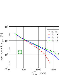
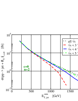
Figure 1: Total jet + nothing cross-section for graviscalar production at LHC to evaluate the validity limit of the phase space volume when: top) only the graviscalar-gluons coupling is present; bottom) only the graviscalar-fermion coupling is present. The curves are normalized to the cross section for graviton production at a value of $E_{T,jet}^{min}$ of 500 GeV.

Notice that these two plots also indicate that for numerically equal couplings, the gluon-graviscalar couplings dominate the cross-section at high energy, while the low-energy regime gets bigger contributions from the quark-graviscalar interactions. This is as expected from the effective Lagrangian, since the gluon terms involve an addition derivative (and so an additional power of $E/M_{D}$ in cross sections) relative to the quark terms.

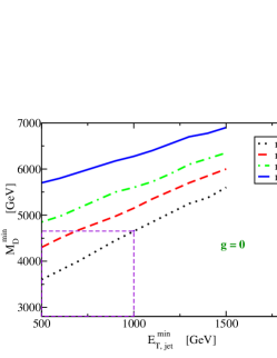
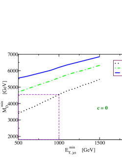
Figure 2: Evaluation of the minimum (4+n)-dimensional Planck scale for which the effective model is valid, at the 90% level, given a cut $E_{T,jet}^{min}$, as explained in the text

For fixed $P_{cut}$, we may ask how large the effective graviscalar couplings may be without introducing more than a 10% error into our calculations. This is illustrated in Figs. (2), which show the smallest value of $M_{D}$ which is permitted given a choice for $E_{T,jet}^{min}=P_{cut}$. This lower bound on $M_{D}$ amounts to choosing an upper bound for the effective dimensional couplings, $\overline{g}$ and $\overline{c}$.

In what follows we calculate the proton-proton cross sections assuming a value for $P_{cut}$, and so the condition $M_{D}>M_{D}^{min}$ determines the domain of validity of our calculations. As discussed above, we determine $M_{D}^{min}$ using gluon-graviscalar couplings, since this is the stronger requirement. From this we find the minimum values for $\overline{g}$ and $\overline{c}$ for which a graviscalar signal would be observable above the statistical Standard Model background at the $5\,\sigma$ level.

4 Simulations

As mentioned above, the processes discussed in Sect. LABEL:sect:processes were implemented using PYTHIA as external processes. Parton flavors were properly assigned in each event according to the CTEQ 5L parton distribution functions evaluated at the renormalization scale $Q^{2}=\frac{1}{2}\,{M^{2}}+p_{T}^{2}$ and the color flow between those parton was applied. ATLAS detector effects were incorporated using the fast Monte Carlo program ATLFAST [15].

For the purpose of comparing with Standard Model backgrounds, we must choose reference values for the couplings $g$ and $c$ as well as for the number of extra dimensions $n$. For these purposes a useful choice is a set of couplings for which the low-energy approximation applies and for which the proton-proton cross section is the same size as the cross-section which was determined as being what is required for a $5\,\sigma$ discovery for graviton production [16]. The reference dimensionless effective couplings, when $P_{cut}=500$ GeV, $M_{D}=5$ TeV and for $n=2$ extra dimensions, are then $g\simeq 0.70$ or $c\simeq 0.41$. These couplings are reasonable from the point of view of the effective theory because the $g$ and $c$ we obtain in this way are smaller than unity. Notice that the existence of such couplings shows that there exist scenarios for which the graviscalar production would be as important as graviton production.

We remark that the following analysis is independent of this choice of reference values.

4.1 Standard Model Backgrounds

If graviscalars are produced in association with a jet in proton collisions the event can be found by searching for a jet plus missing energy: $pp\to\hbox{jet}+\hbox{/\kern-6.69998ptE}_{T}$. The Standard Model background to this process arises from events having neutrinos in the final state. The principal backgrounds of this type and their cross-section in the phase space regions $E_{T,jet}^{min}>500$ GeV and $E_{T,jet}^{min}>1000$ GeV are given, following ref. [16], in Table (1). For comparison, the graviscalar production cross-section using our reference couplings — 2 extra dimensions, $M_{D}=5$ TeV, $E_{T,jet}^{min}=500$ GeV and $(c,g)=(0.41,0.70)$ — is $\sigma=156$ fb.

Processes	cross-section (fb)
	500 GeV	1000 GeV
$pp\rightarrow$jet$+Z(\rightarrow\nu\nu)$	278	6.21
$pp\rightarrow$jet$+W(\rightarrow e\nu_{e})$	364	8.57
$pp\rightarrow$jet$+W(\rightarrow\mu\nu_{\mu})$	364	8.51
$pp\rightarrow$jet$+W(\rightarrow\tau\nu_{\tau})$	363	8.50

Table 1: S.M. background to the graviscalar production at ATLAS and their cross-section for different phase space volume.

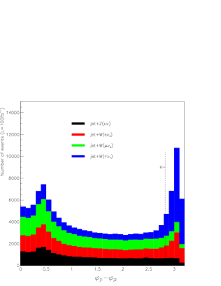
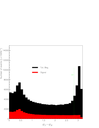
Figure 3: Distribution of the difference in the azimuthal angle between the two most energetic jets of an events for: (top) each of the background; (bottom) the signal and the total background on top of it.

4.2 Analysis

We now determine a set of experimental cuts with which we can find the minimum values of $g$ and $c$ for which a $5\sigma$ discovery is possible. Jets are reconstructed using the cone algorithm with a cone radius $\Delta R=0.4$. In the detector ATLAS, leptons are detected if they are emitted in the range of pseudorapidity $-2.5<\eta<2.5$. Leptons are defined as isolated if the energy deposited by other particles in a cone of radius $\Delta R=\sqrt{(\Delta\phi)^{2}+(\Delta\eta)^{2}}$ is less that 10 GeV. We impose the following two cuts.

As a first cut we require:

Cut 1: No isolated lepton (electron or muon) with $p_{T}>6$ GeV is allowed in the event.

This eliminates most of the $W\to e\nu_{e}$ and $W\to\mu\nu_{\mu}$ events, leaving only those for which the leptons are not properly reconstructed in the detector. It does not eliminate events like $W\to\tau\nu_{\tau}$ in which the $\tau$ decays hadronically, however in this case we expect to also have an energetic low-multiplicity jet which is opposite, in the azimuthal plane, to the principal jet. We see in Fig. (3) that a cut on the difference in azimuthal angle between the two most energetic jets can eliminate a significant fraction of this $\tau$ background.

We therefore impose the second cut:

Cut 2: We keep only events for which $|\varphi_{j_{1}}-\varphi_{j_{2}}|<2.285$ radians.

This cut is chosen to maximize the significance of the remaining signal.

Fig. (4) shows the relative contribution of each process to the total background. After the above cuts, the most important background is $pp\to\hbox{jet}Z\to\hbox{jet}~{}\nu\nu$. Table (2) makes this more explicit, by breaking down the background and comparing it and the signal before and after the cuts are applied, assuming an integrated luminosity of 100 fb^-1. For this integrated luminosity — which corresponds to one year’s running at the nominal LHC luminosity — we therefore expect a total of 36700 background events to remain after cuts.

Processes	$E_{T}^{min}>500$GeV	# events after cut 1	# events after cut 2
jet$+Z(\rightarrow\nu\nu)$	27760	27100	24940
jet$+W(\rightarrow e\nu_{e})$	36420	5224	1430
jet$+W(\rightarrow\mu\nu_{\mu})$	36370	957	866
jet$+W(\rightarrow\tau\nu_{\tau})$	36330	24600	9459
jet+Graviscalar	30960	30090	27720

Table 2: Number of signal ($M_{D}=5$ TeV, $n=2$, $g=0.70$ and $c=0.41$) and background events that survive each cut for an integrated luminosity of 100 fb^-1. The cuts are defined in the text.

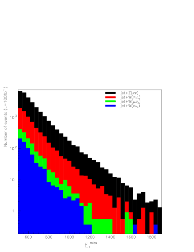
Figure 4: Contributions of different processes to the total background after application of the cuts, for an integrated luminosity of 100 fb^-1.

Is this good enough? We estimate the number of signal events required for a $5\sigma$ discovery using the following significance criterion:

$$\frac{S}{\sqrt{S+B}}>5\,,$$ (12)

where $S$ and $B$ are respectively the number of signal and background events. For this many background events we therefore have a $5\sigma$ discovery if more than 970 graviscalar events are detected, i.e. if the total cross-section for the process is: $\sigma(pp\to\hbox{jet}+\phi)>10.9$ fb. For $n=2$ this corresponds to the effective couplings:

$$\overline{g}>0.18\mathrm{~{}TeV}^{-1}\mathrm{~{}~{}~{}~{}if~{}~{}~{}~{}}\overline{c}=0\,,$$ (13)

or

$$\overline{c}>3.2\times 10^{-1}\mathrm{~{}TeV}^{-2}\mathrm{~{}~{}~{}~{}if~{}~{}~{}~{}}\overline{g}=0\,.$$ (14)

Fig. (5) plots the cross section as a function of missing energy, for two choices of couplings. The choice in the second panel corresponds to the $5\sigma$ discovery limit, and shows that the discovery would be due to an excess of events in the distribution of missing transverse energy at high energies.

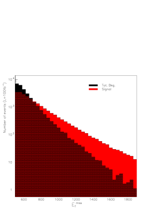
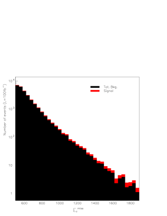
Figure 5: Distribution of missing $E_{T}$ for background and signal when: (top) the cross-section for graviscalar production is the same as the graviton one; (bottom) this cross-section is at its discovery limit.

Notice that the cross section required for discovery is determined by the background rate and so is the same for all choices for $n$, the number of extra-dimensions. In fact, as can be seen in eq. (6), the $\hat{t}$ and $\hat{u}$ dependence of the cross-section does not depend on the number of extra dimensions. Only the effective coupling constants and the energy dependence depend on $n$, through the overall factor $(M^{2})^{({n-2})/{2}}$. Since the angular distribution depends only on $\hat{t}$ and $\hat{u}$, Cut 2 has the same effect for all possible $n$ (as does Cut 1).

4.3 Results

We now turn to the central question: What range of effective couplings are likely to be detectable at the LHC?

We have seen that any determination of the reach of LHC must be made relative to a choice for $E_{T,jet}^{min}=P_{cut}$, since this plays a role in the reliability of the entire theoretical calculation. From Fig. (2) we see that the choice $E_{T,jet}^{min}=500$ GeV implies that the cross-section is sensitive to high-energy parton processes at less than the 10% level, provided $M_{D}\geq M_{D}^{min}$, where $M_{D}^{min}=3.60$, $4.30$, $4.85$ and $5.70$ TeV for $n=2$, 3, 4 and 6 extra dimensions respectively. Given the value for $M_{D}^{min}$ we then determine what values of couplings produce an observably large cross section (i.e. $\sigma>10.9$ fb).

Suppose $(\overline{g}_{obs}^{(n)},\overline{c}_{obs}^{(n)})$ are a pair of dimensionful couplings which each by itself produces a $5\sigma$ signal (in n extra-dimensions) above the Standard Model background. The LHC then can detect couplings which lie in the intervals

$$1\gtrsim g>\overline{g}_{obs}^{(n)}(\overline{M}_{D}^{min})^{{n}/{2}}\mathrm{~{}~{}~{}~{}if~{}~{}~{}~{}}c=0$$

$$\mathrm{or~{}~{}~{}~{}~{}~{}~{}~{}~{}~{}~{}~{}~{}~{}~{}~{}~{}~{}~{}~{}}$$

$$1\gtrsim c>\overline{c}_{obs}^{(n)}(\overline{M}_{D}^{min})^{1+n/2}\mathrm{~{}~{}~{}~{}if~{}~{}~{}~{}}g=0\,.$$

The upper limit in these inequalities expresses the theoretical criterion that the calculation only makes sense below the cut-off scale $M_{D}^{min}$.

Fig. (6) shows the couplings which are accessible if both $c$ and $g$ are simultaneously nonzero. The shaded regions indicate the range of couplings which are too small to have detectable effects for various choices for the dimension $n$. The potentially observationally-interesting couplings are those which lie outside the ellipses, but inside the box defined by $c<1$ and $g<1$. (Recall that since only $c^{2}$ and $g^{2}$ enter into the cross sections, these plots should be interpreted as constraints on $|c|$ and $|g|$.)

We see that whether useful constraints are possible depends on the number of dimensions $n$, and fewer dimensions gives better reach. If $n=2$ couplings outside the innermost region are potentially detectable. For $n=3$ detectable couplings must lie outside the next-to-innermost region. Detection for the case n=4 is unlikely for the dimensionless constant $g$ in the limit of small $c$, but is possible if $c$ is also nonzero. For more then 6 extra dimensions, detection of any signal is unlikely since the minimum value of couplings needed for a discovery when $n=6$ is $(c,g)=(0.9,3.3)$. Any coupling in this region is far enough from the limits of validity of the calculation to have confidence in the result.

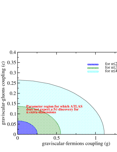
Figure 6: Parameter region for graviscalar theory at second order in $E/M_{D}$ that allow testable and valid physical prediction at ATLAS, for different number of extra-dimension. The graviscalar-fermion and graviscalar-gluon dimensionless couplings are effectively combinations $(g^{2}+g_{5}^{2})^{1/2}$ and $(c^{2}+c_{5}^{2})^{1/2}$

ndim	$M_{D}^{min}$ (TeV)	$M_{D}^{max}$ (TeV)
2	3.2	14.00
3	3.8	6.45
4	4.4	1.45

Table 3: Sensitivity of the ATLAS detector to the fundamental Planck scale $M_{D}$ through the discovery of a graviscalar signal, for $c=0$ and for an integrated luminosity of 100 fb^-1. For $n\geq 4$, observation of a signal is not possible.

An alternative way of expressing the potential ATLAS reach for a graviscalar signal is in terms of the value of the fundamental Planck scale to which the detector might be sensitive. It is bounded on the low side by the requirement that the effective theory be a good approximation, and on the high side by the condition that the signal be detectable. Defining the effective upper limit by

$$M_{D}^{max}=(2\pi)^{\frac{n}{n+2}}\times\min\left[\left(\overline{g}_{obs}^{(n)}\right)^{-2/n},\left(\overline{c}_{obs}^{(n)}\right)^{-2/(n+2)}\right]\,,$$ (15)

there are prospects for detection when $M_{D}^{min}{\ \lower-1.2pt\vbox{\hbox{\hbox to0.0pt{$<$\hss}\lower 5.0pt\vbox{\hbox{$\sim$}}}}\ }M_{D}^{max}$. Table  (3) summarizes these results, with $M_{D}^{max}$ calculated using the worst case: $c=0$.

In the more optimistic limit $g=0$, the maximum value of the fundamental Planck mass to which the ATLAS detector is sensitive increases from 6.45 to 9.50 TeV when $n=3$, and from 1.45 to 7.55 when $n=4$. These results are summarized in Table (4). We again find that $n=6$ is the limiting case since for $g=0$, we have $M_{D}^{max}=5.8$ TeV $\approx M_{D}^{min}=5.7$ TeV.

ndim	$M_{D}^{min}$ (TeV)	$M_{D}^{max}$ (TeV)
2	3.60	14.10
3	4.30	9.50
4	4.85	7.55
6	5.70	5.80

Table 4: Sensitivity of the ATLAS detector to the fundamental Planck scale $M_{D}$ through the discovery of a graviscalar signal, for $g=0$ and for an integrated luminosity of 100 fb^-1. For $n\leq 6$, observation of a signal is possible.

A comparison with the results obtained from graviton emission [16] is also instructive, although some care must be taken in so doing because the graviton results were obtained using a more restrictive phase-space cut ($E_{T}^{min}>1$ TeV), a different criterion for defining the validity region of the model and with a more conservative statistical estimator (${S}>{\sqrt{7B}}$). Tables (5) and (6) compare the sensitivity of ATLAS to $M_{D}$ as computed using graviscalar and graviton production, using these more conservative criteria. The two tables differ in their choice of either $g=0$ or $c=0$.

Table (5) also shows the existing non-accelerator limit on $M_{D}$, taken from ref. [17] (see also [9]). Unlike the situation for gravitons (which couple universally) these astrophysical bounds are more model-dependent when applied to graviscalars. This model dependence arises because they directly bound the couplings of KK modes to electrons and photons, and so need not directly apply to the gluon and quark couplings of most interest for colliders.

c=0	Graviton		Graviscalar		limit from cosmology
	$M_{D}^{min}$	$M_{D}^{max}$	$M_{D}^{min}$	$M_{D}^{max}$	$M_{D}^{min}$ (A)	$M_{D}^{min}$ (B)
n=2	$\sim$4.0 TeV	7.5 TeV	4.35 TeV	5.45 TeV	O(90) TeV	$\sim 10$ TeV
n=3	$\sim$4.5	5.9	4.85	3.65	5.0	0.8
n=4	$\sim$5.0	5.3	5.35	3.20	$\lesssim 4$	$\lesssim 1$

Table 5: With c=0: comparison of the sensitivity of ATLAS to $M_{D}$ for graviscalar and graviton signals under the conditions $E_{T}^{min}>1$TeV, $\frac{S}{\sqrt{7B}}$ and with indirect constaints from cosmology. The integrated luminosity is 100 fb^-1. For $n\geq 3$, observation of a graviscalar signal is not possible since $M_{D}^{min}>M_{D}^{max}$. For the cosmology bounds, Scenario A means limits to neutron star heating by KK-decays, while scenario B corresponds to bounds from the cooling of SN1987A by KK-mode emission.

g=0	Graviton		Graviscalar
	$M_{D}^{min}$	$M_{D}^{max}$	$M_{D}^{min}$	$M_{D}^{max}$
n=2	$\sim$4.0 TeV	7.5 TeV	4.65 TeV	10.20 TeV
n=3	$\sim$4.5	5.9	5.15	7.75
n=4	$\sim$5.0	5.3	5.60	6.50

Table 6: With g=0: comparison of the sensitivity of ATLAS to $M_{D}$ for graviscalar and graviton signals under the consitions $E_{T}^{min}>1$TeV, $\frac{S}{\sqrt{7B}}$ and with indirect constaints from cosmology. The integrated luminosity is 100 fb^-1. For $n\leq 4$, observation of a graviscalar signal is possible.

We see again that the scenario where $g\to 0$ gives the best case for detection, and this is competitive with the graviton result. We also see that although accelerator experiments are most sensitive to lower $n$, for quark couplings these may be pre-empted by the non-accelerator bounds.

The difference between the cases $c=0$ and $g=0$ show that ATLAS is likely to be only weakly sensitive to the graviscalar Yukawa couplings (especially keeping in mind these are naturally expected to be at most of order $v/\overline{M}_{D}$, as explained in section 2), and a discovery is more likely to come from gluon-graviscalar couplings. However, once a signal is seen we are unlikely to be able to decide directly on the relative importance between $g$ and $c$. Therefore, even if the discovery of a significant graviscalar signal at ATLAS should turn out to be possible, it is unlikely to completely fix its couplings.

4.4 Graviton-Graviscalar Confusion

Should a missing-energy signal be seen at the LHC, how does one tell if it is due to gravitons or graviscalars? We do not yet see a way to do so, despite the difference in their spin, for the following reasons.

• The graviscalar production cross-section has an energy dependence which is similar to the graviton one, precluding the use of $P_{T,jet}$, $\hbox{/\kern-6.69998ptE}_{T}$ or any other function of energy to discriminate the two.

• Parton-level discriminants are not likely to be of practical use, because the center of mass energy of the hard scattering is not known in a $pp$ collider such as the LHC. Furthermore, the final state we consider consists of a single jet and missing transverse energy, so it is not possible to reconstruct the longitudinal component of momentum of the system of interacting partons, nor their angular distribution in the center of mass, nor their forward-backward asymmetry. Even if this were possible, we have checked that the discrimination between the shapes of the graviscalar and graviton differential cross sections is difficult even at the purely theoretical parton level. Only gluon fusion processes lead to a small difference.

5 Conclusions

We have computed the rate for the production of extra-dimensional scalars (as opposed to components of extra-dimensional tensors which look at low energies like 4D scalars) in $pp$ collisions. Such particles arise in virtually all supersymmetric higher-dimensional theories, and our work complements previous studies of gravitons [4, 16] and of extra-dimensional vectors [9]. Because of the way we compute our phase space integrals, our study applies to large-extra-dimensional (ADD-type) models and not to warped (RS-type) models.

We find that the cross sections for the reaction $pp\to\phi+\hbox{jet}$ are similar in size and shape to those for graviton production, although the competing non-accelerator constraints on the couplings can differ because graviscalars need not couple universally (unlike gravitons). We used simulation codes tailored to the ATLAS detector, and conclude that ATLAS can be sensitive to graviscalar couplings, provided there are less than 6 extra dimensions. The sensitivity improves with fewer dimensions, although so does the restrictiveness of non-accelerator bounds on the extra-dimensional Planck scale. Nontrivial windows of opportunity can be consistent with all bounds.

Generically, $pp$ collisions are more sensitive to graviscalar couplings to gluons than they are to couplings to quarks. Both couplings are turned on in our analysis, and we find that observable quark couplings often push the limits of validity of the effective-field-theory description.

6 Acknowledgements

This work has been performed within the ATLAS collaboration. We have made use of physics analysis and simulation tools which are the result of collaboration-wide efforts. We would like to acknowledge partial funding from NSERC (Canada). C.B. research is partially funded by FCAR (Québec) and McGill University.

7 Appendix

To proceed the cross sections, we require the Feynman rules for the $\bar{q}q\phi$, $gg\phi$ and $ggg\phi$ vertices which follow from the effective lagrangian of eq. (2), which are:

$=-i(\overline{g}+i\overline{g}_{5}\gamma_{5})$

$=4i[\overline{c}(p.q)g_{\mu\nu}-\overline{c}p_{\mu}q_{\nu}-\overline{b}\epsilon_{\mu\nu\alpha\beta}p^{\alpha}q^{\beta}]\delta_{ab}$

$=4g_{3}f^{abc}[\overline{c}g_{\mu\nu}(p_{\rho}-q_{\rho})+\overline{c}g_{\mu\rho}(k_{\nu}-p_{\nu})+\overline{c}g_{\nu\rho}(q_{\mu}-k_{\mu})-\overline{b}\epsilon_{\alpha\mu\nu\rho}(p^{\alpha}+q^{\alpha}+k^{\alpha})]$

Figure 7: The parton-level Feynman graphs which contribute to graviscalar production with an associated jet in proton-proton scattering.

References

- [1] E. Witten, Nucl. Phys. B471 (1996) 135 (hep-th/9602070); J. Lykken, Phys. Rev. D54 (1996) 3693 (hep-th/9603133); P. Horava and E. Witten, Nucl. Phys. B475 (1996) 94 (hep-th/9603142); I. Antoniadis, N. Arkani-Hamed, S. Dimopoulos and G. Dvali, Phys. Lett. B436 (1998) 257 (hep-ph/9804398); Nucl. Phys. B460 (1996) 506 (hep-th/9510209); I. Antoniadis, Phys. Lett. B246 (1990) 377.
- [2] N. Arkani-Hamed, S. Dimopoulos and G. Dvali, Phys. Lett. B429 (1998) 263 (hep-ph/9803315); Phys. Rev. D59 (1999) 086004 (hep-ph/9807344).
- [3] L. Randall, R. Sundrum, Phys. Rev. Lett. 83 (1999) 3370 [hep-ph/9905221], Phys. Rev. Lett. 83 (1999) 4690 [hep-th/9906064].
- [4] Real graviton emission is discussed in G. F. Giudice, R. Rattazzi and J. D. Wells, Nucl. Phys. B544, 3 (1999) [hep-ph/9811291]; E. A. Mirabelli, M. Perelstein and M. E. Peskin, Phys. Rev. Lett. 82, 2236 (1999) [hep-ph/9811337]; T. Han, J. D. Lykken and R. Zhang, Phys. Rev. D59, 105006 (1999) [hep-ph/9811350]; K. Cheung and W.-Y. Keung, Phys. Rev. D60, 112003 (1999) [hep-ph/9903294]; S. Cullen and M. Perelstein, Phys. Rev. Lett. 83 (1999) 268 [hep-ph/9903422]; C. Balázs et al., Phys. Rev. Lett. 83 (1999) 2112 [hep-ph/9904220]; L3 Collaboration (M. Acciarri et al.), Phys. Lett. B464, 135 (1999), [hep-ex/9909019], Phys. Lett. B470, 281 (1999) [hep-ex/9910056].
- [5] There is an extensive literature examining the effects of virtual graviton exchange. For a review, along with a comprehensive list of references, see K. Cheung, talk given at the 7th International Symposium on Particles, Strings and Cosmology (PASCOS 99), Tahoe City, California, Dec 1999, hep-ph/0003306.
- [6] E. Accomando, I. Antoniadis and K. Benakli, Nucl. Phys. B579, 3 (2000) [hep-ph/9912287]; S. Cullen, M. Perelstein and M. E. Peskin, [hep-ph/0001166].
- [7] Y. Aghababaie, C.P. Burgess, J.M. Cline, H. Firouzjahi, S. Parameswaran, F. Quevedo, G. Tasinato and I. Zavala C., [hep-th/0308064].
- [8] Y. Aghababaie, C.P. Burgess, S. Parameswaran and F. Quevedo, [hep-th/0304256].
- [9] D. Atwood, C.P. Burgess, E. Filotas, F. Leblond, D. London and I. Maksymyk, Physical Review D63 (2001) 025007 [hep-ph/0007178].
- [10] G. Giudice, R. Rattazzi and J.D. Wells, Nucl. Phys. B595 (2001) 250, [hep-ph/0002178].
- [11] C.P. Burgess, Q. Matias and M. Pospelov, I.J.M.P. A17 (2002) 1841–1918, (hep-ph/9912459).
- [12] C.P. Burgess, Phys. Rep. C330 (2000) 193 (hep-th/9808176).
- [13] F. Leblond, Phys.Rev. D64 (2001) 045016 [hep-ph/0104273]
- [14] T. Sjöstrand et.al., Comp. Phys. Comm. 135 (2001) 238.
- [15] E. Richter-Was, D. Froidevaux, L. Poggioli, ATLFAST 2.0, a fast simulation package for ATLAS, ATLAS-PHYS-98-131
- [16] L. Vacavant and I. Hinchliffe, J. Phys., G : 27 (2001) 1839 and ATL-PHYS-2000-016
- [17] J. Hewett and J. March-Russell, in Review of Particle Physics, K. Hagiwara et al. (Particle Data Group), Phys. Rev. D 66, 010001 (2002) [http://pdg.lbl.gov]; S. Hannestad and G. Raffelt, Phys.Rev.Lett. 88 (2002) 071301 [hep-ph/0110067]