The $B^{-}\to\phi\phi K^{-}$ decay rate with $\phi\phi$ invariant mass below charm threshold

S. Fajfer^a,b, T.N. Pham^c, A. Prapotnik^b

a) Department of Physics, University of Ljubljana, Jadranska 19, 1000 Ljubljana, Slovenia

b) J. Stefan Institute, Jamova 39, P. O. Box 300, 1001 Ljubljana, Slovenia

c) Centre de Physique Teorique, Centre National de la Recherche Scientifique, UMR 7644, Ecole Polytechnique, 91128 Palaiseau Cedex, France

ABSTRACT

We investigate the decay mechanism in the $B^{-}\to\phi\phi K^{-}$ decay with the $\phi\phi$ invariant mass below the charm threshold and in the neighborhood of the $\eta_{c}$ invariant mass region. Our approach is based on the use of factorization model and the knowledge of matrix elements of the weak currents. For the $B$ meson weak transition we apply form factor formalism, while for the light mesons we use effective weak and strong Lagrangians. We find that the dominant contributions to the branching ratio come from the $\eta$, $\eta^{\prime}$ and $\eta(1490))$ pole terms of the penguin operators in the decay chains $B^{-}\to\eta(\eta^{\prime},\eta(1490))K^{-}\to\phi\phi K^{-}$. Our prediction for the branching ratio is in agreement with the Belle’s result.

I. INTRODUCTION

It is a very fruitful era in $B$ meson physics. A lot of experimental data on $B$ meson decays is coming from the $B$ meson factories. Many of their results are still not explained. Recently, Belle collaboration has announced the observation of the ${\rm BR}(B^{\pm}\to\phi\phi K^{\pm})=$ $(2.6^{+1.1}_{-0.9}\pm 0.3)\times 10^{-6}$ [1] for a $\phi\phi$ invariant mass below $2.85\,$GeV. This is the first of the three-body $B$ decays with two vector mesons and one pseudoscalar meson in the final state that has been observed. The $B$ meson decays into three pseudoscalar mesons have been studied [2, 3] within heavy quark symmetry accompanied by chiral symmetry. One might explain the observed rates using heavy quark symmetry for the strong vertices, while for the weak transition we rely on the existing knowledge of the form factors [2]. The three-body decay with two vector meson states and one pseudoscalar is much more difficult to approach.

The additional insight on the decay mechanism might come from the analysis of the $B$ meson two-body decays. Particularly interesting are the decays $B^{\pm}\to\phi K^{\pm}$, $B^{\pm}\to$ $\eta(\eta^{\prime})K^{\pm}$ and $B\to K^{*\pm}\phi$. They have been extensively studied using different existing techniques: the naive factorization [4, 5, 6], the QCD factorization [7] and the SU(3) symmetry [8]. Each of these decay modes is rather difficult to explain theoretically. The decays $B^{\pm}\to\phi K^{\pm}$ and $B^{\pm}\to K^{*\pm}\phi$ might have significant annihilation contribution [4, 6, 9], but it is not simple to have a consistent treatment of it. There is an interesting proposal [6] in which the angular distributions of the final outgoing particles can be used to estimate the magnitude of annihilation contribution to the amplitude. However, we have to wait for the new experimental data to extract the size of the annihilation contribution. The $B^{\pm}\to\eta(\eta^{\prime})K^{\pm}$ decay rate has not been easy to explain. It accounts for the well-known problem of the $\eta-\eta^{\prime}$ mixing [10, 11] as can be seen from a variety of approaches used for $B^{\pm}\to\eta(\eta^{\prime})K^{\pm}$ [4, 12, 13, 14]. In the $B^{\pm}\to\eta(\eta^{\prime})K^{\pm}$ decay mode, it seems that the annihilation contribution is not very significant [4, 13].

One has to expect that the above described difficulties in these decay modes might appear in the three-body decay we discuss. Based on the current knowledge of two-body transitions, we build a simple model which might clarify the role of the non-charm contributions in the ${\rm BR}(B^{\pm}\to\phi\phi K^{\pm})$ decay. In our study of the $B^{\pm}\to\phi\phi K^{\pm}$ decay mechanism, we follow the assumption in ref. [2] and use double and single pole form factors for the $B$ meson semileptonic transitions [15, 16]. Our approach is based on naive factorization, as QCD factorization has not been developed yet for three-body decays. The $SU(3)$ symmetry approach is not applicable due to the limited number of the observed $B$ decay modes. In our model we keep only dominant contributions and as in the case of two-body charmless $B$ decays, we do not include annihilation contributions. We use a pole model including the low-lying meson resonances and possible contributions coming from higher mass excited states.

In order to compare our result with the Belle’s result, we include in our calculation the interference between the non-resonant $B^{-}\to K^{-}\phi\phi$ and the resonant $B^{-}\to K^{-}\eta_{c}\to K^{-}\phi\phi$ decay amplitude.

In Section II we present the basic elements of our model, while in Section III we give the results for the three-body decay amplitude and discuss possible contributions to the decay rate.

II. THE MODEL

The $\bar{u}b\to s\bar{u}\bar{s}s$ transition which can produce two $\phi$ mesons in the final state via strong interactions, can be realized by the effective weak Hamiltonian [17]-[20]:

$${\cal H}_{eff}=\frac{G_{F}}{\sqrt{2}}\left([V_{ub}V^{*}_{us}(c_{1}O_{1u}+c_{2}O_{2u})-\sum^{10}_{i=3}[(V_{ub}V^{*}_{us}c^{u}_{i}+V_{cb}V^{*}_{cs}c^{c}_{i}+V_{tb}V^{*}_{ts}c^{t}_{i})O_{i}]\right),$$ (1)

where $O_{1}$ and $O_{2}$ are the tree-level operators, $O_{3}-O_{6}$ are gluonic penguin operators and $O_{7}-O_{10}$ are electroweak penguin operators. Superscripts $u,c,t$ on the Wilson coefficients denote the internal quark in penguin loop. In order to apply the factorization approximation we rearrange the above operators using Fierz transformations and leave only color-singlet ones. One then comes to the effective weak Hamiltonian given by Eq. (1) replacing the coefficients $c_{i}$ by $a_{i}$. The relevant operators are:

$$\begin{array}[]{l}{\cal O}_{1}=(\bar{u}b)_{V-A}(\bar{s}u)_{V-A},\\ {\cal O}_{2}=(\bar{s}b)_{V-A}(\bar{u}u)_{V-A},\\ {\cal O}_{3}=\sum_{q}{\cal O}^{q}_{3}=\sum_{q}(\bar{s}b)_{V-A}(\bar{q}q)_{V-A},\\ {\cal O}_{4}=\sum_{q}{\cal O}^{q}_{4}=\sum_{q}(\bar{s}q)_{V-A}(\bar{q}b)_{V-A},\\ {\cal O}_{5}=\sum_{q}{\cal O}^{q}_{5}=\sum_{q}(\bar{s}b)_{V-A}(\bar{q}q)_{V+A},\\ {\cal O}_{6}=-2\sum_{q}{\cal O}^{q}_{6}=-2\sum_{q}(\bar{s}(1+\gamma_{5})q)(\bar{q}(1-\gamma_{5})b),\\ {\cal O}_{7}=\sum_{q}{\cal O}^{q}_{7}=\sum_{q}\frac{3}{2}e_{q}(\bar{s}b)_{V-A}(\bar{q}q)_{V+A},\\ {\cal O}_{8}=-2\sum_{q}{\cal O}^{q}_{8}=-2\sum_{q}\frac{3}{2}e_{q}(\bar{s}(1+\gamma_{5})q)(\bar{q}(1-\gamma_{5})b),\\ {\cal O}_{9}=\sum_{q}{\cal O}^{q}_{9}=\sum_{q}\frac{3}{2}e_{q}(\bar{s}b)_{V-A}(\bar{q}q)_{V-A},\\ {\cal O}_{10}=\sum_{q}{\cal O}^{q}_{10}=\sum_{q}\frac{3}{2}e_{q}(\bar{s}q)_{V-A}(\bar{q}b)_{V-A},\end{array}$$ (2)

The Wilson coefficients are taken from [19]:

$$\begin{array}[]{lll}a_{1}=1.05,&a_{2}=0.07,&a_{3}=47\times 10^{-4},\\ a_{4}=(-43-16i)\times 10^{-3},&a_{5}=-53\times 10^{-4},&a_{6}=(-54-16i)\times 10^{-3},\\ a_{7}=(0.4-0.9i)\times 10^{-4},&a_{8}=(3.3-0.3i)\times 10^{-4},&a_{9}=(-91-0.9i)\times 10^{-4},\\ &a_{10}=(-13-0.3i)\times 10^{-4}.&\\ \end{array}$$ (3)

For the CKM matrix elements ($V_{ij}$) we use Wolfenstein parametrization:$V_{tb}V^{*}_{ts}=-A\lambda^{2}$ and $V_{ub}V^{*}_{us}=A\lambda^{4}(\bar{\rho}-i\bar{\eta})$, where $A=0.83$, $\lambda=0.222$, $\bar{\rho}=0.217/(1-\lambda^{2}/2)$ and $\bar{\eta}=0.331/(1-\lambda^{2}/2)$. The standard decomposition of the weak current matrix elements is:

$$\langle V(k,\varepsilon,m_{V})|\bar{q}\Gamma^{\mu}q|P(p,M)\rangle=\epsilon^{\mu\nu\alpha\beta}\varepsilon_{\nu}p_{\alpha}k_{\beta}\frac{2V(q^{2})}{M+m_{V}}+2im_{V}\frac{\varepsilon\cdot q}{q^{2}}q^{\mu}A_{0}(q^{2})$$

$$+i(M+m_{V})\Big{[}\varepsilon^{\mu}-\frac{\varepsilon\cdot q}{q^{2}}q^{\mu}\Big{]}A_{1}(q^{2})-i\frac{\varepsilon\cdot q}{M+m_{V}}\Big{[}P^{\mu}-\frac{M^{2}-m_{V}^{2}}{q^{2}}q^{\mu}\Big{]}A_{2}(q^{2})\;,$$ (4)

$$\langle P(k,m_{P})|\bar{q}\Gamma^{\mu}q|P(p,M)\rangle=\left(P^{\mu}-\frac{(M^{2}-m_{P}^{2})}{q^{2}}q^{\mu}\right)F_{+}(q^{2})+\frac{(M^{2}-m_{P}^{2})}{q^{2}}q^{\mu}F_{0}(q^{2})\;,$$ (5)

where $q^{\mu}=p^{\mu}-k^{\mu}$ and $P^{\mu}=p^{\mu}+k^{\mu}$. Also

$$\langle P(p)|\bar{q}\gamma^{\mu}(1-\gamma_{5})q|0\rangle=if_{P}p^{\mu}\;,\qquad\langle 0|\bar{q}\gamma^{\mu}q|V(p)\rangle=g_{V}\varepsilon^{\mu}\;.$$ (6)

Using experimental data [21], the decay constants are found to be $|g_{\phi}|=0.24\,$GeV², $|g_{K}|=0.19\,$GeV², $f_{K}=0.16\,$GeV and $f_{\pi}=0.132\,$GeV. The lattice calculation [22] gives for the $B$ meson decay constants $f_{B}=0.173\,$GeV and $f_{B_{s}}=1.22f_{B}$. We also take $g_{B^{*}}=M_{B^{*}}f_{B}$ [16]. The $q^{2}$ dependence of the form factors is studied in [16], where a quark model is combined with a fit to lattice and experimental data. This approach results in a double pole $q^{2}$ dependence of $F_{+}(q^{2})$, $V(q^{2})$ and $A_{0}(q^{2})$

$$f(q^{2})=\frac{f(0)}{(1-q^{2}/M^{2})(1-\sigma_{1}q^{2}/M^{2}+\sigma_{2}q^{4}/M^{4})}\;,$$ (7)

while for $A_{1,2}(q^{2})$ and $F_{0}(q^{2})$ [16] we have:

$$f(q^{2})=\frac{f(0)}{(1-\sigma q^{2}/M^{2}+\sigma_{2}q^{4}/M^{4})}\;.$$ (8)

Values of $M$, $f(0)$, $\sigma_{1}$ and $\sigma_{2}$ are listed in Table 1.

form factor	$F_{+}$	$F_{0}$	$V$	$A_{0}$	$A_{1}$	$A_{2}$
$f(0)$	0.36	0.36	0.44	0.45	0.36	0.32
$\sigma_{1}$	0.43	0.70	0.45	0.46	0.64	1.23
$\sigma_{2}$	0.0	0.27	0.0	0.0	0.36	0.38
$M$ [GeV]	5.42	5.42	5.42	5.37	5.42	5.42

Table 1: The $B\to K,K^{*}$ form factors at $q^{2}=0$ and the pole parameters [16].

In the evaluation of ${\cal O}_{6}$ operator we have as usual [13]

$$\bar{q}_{1}\gamma_{5}q_{2}=\frac{-i}{m_{1}+m_{2}}\partial_{\mu}(\bar{q}_{1}\gamma^{\mu}\gamma_{5}q_{2})\,,$$ (9)

$$\bar{q}_{1}q_{2}=\frac{-i}{m_{1}-m_{2}}\partial_{\mu}(\bar{q}_{1}\gamma^{\mu}q_{2})\,.$$ (10)

The effects of strong interactions of light mesons are taken into account by using the following effective Lagrangian [23, 24, 25]:

$${\cal L}_{\rm strong}=\frac{ig_{\rho\pi\pi}}{{\sqrt{2}}}Tr(\rho^{\mu}[\Pi,\partial_{\mu}\Pi])-4\frac{C_{VV\Pi}}{f}\epsilon^{\mu\nu\alpha\beta}Tr(\partial_{\mu}\rho_{\nu}\partial_{\alpha}\rho_{\beta}\Pi)\;,$$ (11)

where $\Pi$ and $\rho^{\mu}$ are $3\times 3$ matrices containing pseudoscalar and vector meson field operators respectively and $f$ is a pseudoscalar meson decay constant as in Eq. (6). We take $C_{VV\Pi}=0.31$ [26]. In order to include SU(3) flavor symmetry breaking, instead of the coupling constant coming from the $\rho\to\pi\pi$ decay ($g_{\rho\pi\pi}=5.9$), we use the coupling constant coming from the $\phi\to KK$ decay rate. Thus, we have $g_{\phi KK}=6.4$.

For the description of strong interactions between heavy and light mesons, we use definitions given in [16] and heavy quark effective theory to get:

$$<K(p_{1})B^{*}_{s}(p_{2},\varepsilon)|B(p_{1}+p_{2})>=\frac{g_{B_{s}^{*}BK}}{2}(p_{1}+2p_{2})_{\mu}\varepsilon^{\mu}\,,$$ (12)

$$<\phi(p_{1},\varepsilon_{1})B^{*}_{s}(p_{2},\varepsilon_{2})|B^{*}_{s}(p_{1}+p_{2},\varepsilon)>=\frac{1}{2}g_{B_{s}B_{s}\phi}(p_{1}\cdot\varepsilon_{2}\,\varepsilon_{1}\cdot\varepsilon-p_{1}\cdot\varepsilon\,\varepsilon_{2}\cdot\varepsilon_{1})\,,$$ (13)

where $g_{B_{s}B_{s}\phi}f_{B_{s}}/2m_{\phi}=1.5\pm 0.1$ and $g_{B^{*}_{s}BK}f_{B_{s}}/2m_{B_{s}^{*}}=0.65\pm 0.05$ [16].

To account for the $\eta-\eta^{\prime}$ mixing, we follow the approach in [11]. Using the quark basis ($\eta_{q}\simeq(u\bar{u}+d\bar{d})/{\sqrt{2}}$ and $\eta_{s}\simeq s\bar{s}$), the mixing is given by

$${\eta\choose\eta^{\prime}}=\left(\begin{array}[]{cc}\cos\phi&-\sin\phi\\ \sin\phi&\cos\phi\end{array}\right){\eta_{q}\choose\eta_{s}}\,,$$ (14)

with the mixing angle $\phi=39.3^{\circ}\pm 1.0^{\circ}$. The $\eta$, $\eta^{\prime}$ decay constants are defined by

$$<\eta|\bar{q}\gamma^{\mu}(1-\gamma_{5})q|0>=if^{q}_{\eta}\,,\qquad<\eta^{\prime}|\bar{q}\gamma^{\mu}(1-\gamma_{5})q|0>=if^{q}_{\eta^{\prime}}\,,$$ (15)

where

$$\begin{array}[]{ll}f^{u,d}_{\eta}=f_{u,d}\cos\phi/\sqrt{2}\,,&f^{s}_{\eta}=-f_{s}\sin\phi\,,\\ f^{u,d}_{\eta^{\prime}}=f_{u,d}\sin\phi/\sqrt{2}\,,&f^{s}_{\eta^{\prime}}=f_{s}\cos\phi\,,\end{array}$$ (16)

with $f_{u,d}=(1.07\pm 0.02)f_{\pi}$ and $f_{s}=(1.34\pm 0.06)f_{\pi}$. The form factors for the $B\to\eta(\eta^{\prime})$ transition can be written as:

$$F^{\eta}_{0,+}(q^{2})=F^{\pi}_{0}(q^{2})\cos\phi/\sqrt{2}\,,\qquad F^{\eta^{\prime}}_{0,+}(q^{2})=F^{\pi}_{0}(q^{2})\sin\phi/\sqrt{2}\,.$$ (17)

The $q^{2}$ dependence of $F^{\pi}_{0}$ is described by Eq. (8), with $F^{\pi}_{0}(0)=0.29$, $\sigma_{1}=0.76$ and $\sigma_{2}=0.28$ while the $q^{2}$ dependence of $F^{\pi}_{+}$ is described by Eq. (7), with $F^{\pi}_{+}(0)=0.29$ and $\sigma_{1}=0.48$ [16].

Before we consider the $B^{-}\to\phi\phi K^{-}$ decay amplitude, we check how our model works for the two-body decays: $B^{-}\to\eta K^{-}$, $B^{-}\to\eta^{\prime}K^{-}$, $B^{-}\to\phi K^{-}$, and $B^{-}\to\phi K^{*-}$. Namely, $B^{-}\to\phi\phi K^{-}$ can occur through one of these decay chains: $B^{-}\to\eta(\eta^{\prime})K^{-}$ followed by $\eta(\eta^{\prime})\to\phi\phi$; $B^{-}\to\phi K^{-}$, followed by $K^{-}\to K^{-}\phi$ and $B^{-}\to\phi K^{*-}$ followed by $K^{*-}\to K^{-}\phi$. These decays have already been studied within the factorization approximation by Ali et. al. [4]. Using their formulas for the amplitudes with the Wilson coefficients, the form factors and other parameters as given above, we obtain the branching ratios for the two-body decays presented in Table 2 together with the experimental results. We point out that references [4, 14], as well as our predictions, include the axial anomaly contribution in $b\to sgg\to s\eta(\eta^{\prime})$. In our calculation, the contribution of the $\bar{c}c$ component in $\eta,\eta^{\prime}$ was found to be small and therefore we safely neglect it.

	Belle [27, 28]	BaBar [29, 30, 31, 32]	our model
$B^{-}\to\eta K^{-}$	$(5.3^{+1.8}_{-1.5}\pm 0.6)\times 10^{-6}$	$(2.8^{+0.8}_{-0.7}\pm 0.2)\times 10^{-6}$	$2.1\times 10^{-6}$
$B^{-}\to\eta^{\prime}K^{-}$		$(7.67\pm 0.35\pm 0.44)\times 10^{-5}$	$3.0\times 10^{-5}$
$B^{-}\to\phi K^{-}$	$(9.4\pm 1.1\pm 0.7)\times 10^{-6}$	$(10^{+0.9}_{-0.8}\pm 0.5)\times 10^{-6}$	$14.9\times 10^{-6}$
$B^{-}\to\phi K^{*-}$	$(6.7^{+2.1+0.7}_{-1.5-0.8})\times 10^{-6}$	$(12.7^{+2.2}_{-2.0}\pm 1.1)\times 10^{-6}$	$8.6\times 10^{-6}$

Table 2: The experimental and theoretical results for the relevant $B^{-}$ two-body decay rates. The rates for $B^{-}\to\eta K^{-}$ and $B^{-}\to\eta^{\prime}K^{-}$ are calculated without $c\bar{c}$ contributions.

III. THE $B^{-}\to\phi\phi K^{-}$ DECAYS

Figure 1: Feynman diagrams for $B^{-}\to\phi\phi K^{-}$.

The dominant contributions in the $B^{-}(p)\to K^{-}(p_{1})\phi(p_{2})\phi(p_{3})$ decay amplitude with the $\phi\phi$ invariant mass in the region below the charm threshold are shown in Fig. 1. We write the amplitude for this decay in the following form:

$${\cal M}={\cal A}_{1}\left(\sum_{q=s,u,d}C^{\eta}_{1q}\right)+{\cal A}_{2}\left(\sum_{q=s,u,d}C^{\eta^{\prime}}_{1q}\right)+{\cal A}_{3}C^{\eta}_{2}+{\cal A}_{4}C^{\eta^{\prime}}_{2}+({\cal A}_{5}+{\cal A}_{6}+{\cal B})C^{K}_{1}\,.$$ (18)

Here

$$C^{\eta}_{1u}=\frac{G_{F}}{\sqrt{2}}\left(V_{ub}V^{*}_{us}a_{2}-V_{tb}V^{*}_{ts}(a_{3}-a_{5}+a_{9}-a_{7})\right)\frac{f^{u}_{\eta}}{f_{\pi}}\,,$$

$$C^{\eta}_{1d}=-\frac{G_{F}}{\sqrt{2}}V_{tb}V^{*}_{ts}(a_{3}-a_{5}-1/2(a_{9}-a_{7}))\frac{f^{d}_{\eta}}{f_{\pi}}\,,$$

$$C^{\eta}_{1s}=-\frac{G_{F}}{\sqrt{2}}V_{tb}V^{*}_{ts}\left(\left(a_{3}+a_{4}-a_{5}-1/2(a_{9}+a_{10}-a_{7})+\frac{p^{2}_{\eta}}{m_{b}m_{s}}(a_{6}-1/2a_{8})\right)\frac{f^{s}_{\eta}}{f_{\pi}}-\right.$$

$$\left.\frac{p^{2}_{\eta}}{m_{b}m_{s}}(a_{6}-1/2a_{8})\frac{f^{u}_{\eta}}{f_{\pi}}\right)\,,$$ (19)

$$C^{\eta}_{2}=\frac{G_{F}}{\sqrt{2}}V_{ub}V^{*}_{us}a_{1}-V_{tb}V^{*}_{ts}(a_{4}+a_{10}+\frac{2p^{2}_{K}}{m_{b}m_{s}}(a_{6}+a_{8}))\,,$$

$$C^{K}_{1}=\frac{G_{F}}{\sqrt{2}}(-V_{tb}V^{*}_{ts})\big{(}a_{3}+a_{4}+a_{5}-1/2(a_{7}+a_{9}+a_{10})\big{)}\,,\qquad$$ (20)

where $p_{\eta}$ and $p_{K}$ are the momenta of $\eta$ and $K$ meson respectively. The formulas for $\eta^{\prime}$ are obtained by replacing $f^{q}_{\eta}$ and $k_{s}$ with $f^{q}_{\eta^{\prime}}$ and $k^{\prime}_{s}$. The constant $k_{s}$ ($k^{\prime}_{s}$) projects the $\bar{s}s$ component of the $\eta$ ($\eta^{\prime}$) meson and it is equal $-\sin\phi$ for $\eta$ and $\cos\phi$ for $\eta^{\prime}$. The coefficient $C_{1s}^{\eta}$ contains the effect of the axial anomaly as in [4, 14]. The amplitudes are determined by

$${\cal A}_{1}=8iC_{VV\Pi}k_{s}F_{0}(x)\frac{M^{2}-m_{K}^{2}}{m^{2}_{\eta}-x}\epsilon_{\mu\nu\alpha\beta}\varepsilon^{\mu}_{2}\varepsilon^{\nu}_{3}p_{2}^{\alpha}p_{3}^{\beta}\,,$$ (21)

$${\cal A}_{2}=8iC_{VV\Pi}k_{s}F_{0}(x)\frac{M^{2}-m_{K}^{2}}{m^{2}_{\eta^{\prime}}-x}\epsilon_{\mu\nu\alpha\beta}\varepsilon^{\mu}_{2}\varepsilon^{\nu}_{3}p_{2}^{\alpha}p_{3}^{\beta}\,,$$ (22)

$${\cal A}_{3}=8iC_{VV\Pi}\frac{f_{K}}{f_{\pi}}\big{(}F^{\eta}_{0}(m_{K}^{2})\frac{M^{2}-m^{2}_{\eta}}{m^{2}_{\eta}-x}+F^{\eta}_{+}(m_{K}^{2})\big{)}\epsilon_{\mu\nu\alpha\beta}\varepsilon^{\mu}_{2}\varepsilon^{\nu}_{3}p_{2}^{\alpha}p_{3}^{\beta}\,,$$ (23)

$${\cal A}_{4}=8iC_{VV\Pi}\frac{f_{K}}{f_{\pi}}\big{(}F^{\eta^{\prime}}_{0}(m_{K}^{2})\frac{M^{2}-m^{2}_{\eta^{\prime}}}{m^{2}_{\eta^{\prime}}-x}+F^{\eta^{\prime}}_{+}(m_{K}^{2})\big{)}\epsilon_{\mu\nu\alpha\beta}\varepsilon^{\mu}_{2}\varepsilon^{\nu}_{3}p_{2}^{\alpha}p_{3}^{\beta}\,,$$ (24)

$${\cal A}_{5}=2\sqrt{2}g_{\phi}g_{\rho\pi\pi}F_{+}(m_{\phi}^{2})\left(\frac{p_{1}\cdot\varepsilon_{2}\,p\cdot\varepsilon_{3}}{m_{K}^{2}-y}+\frac{p\cdot\varepsilon_{2}\,p_{1}\cdot\varepsilon_{3}}{x+y-M^{2}-2m_{\phi}^{2}}\right)\,,$$ (25)

$${\cal A}_{6}=-\frac{2g_{\phi}C_{VV\Pi}}{f_{K}(M+m_{K^{*}})}\left(2i(M+m_{K^{*}})^{2}A_{1}(m_{\phi}^{2})\left(\frac{\epsilon_{\mu\nu\alpha\beta}\varepsilon^{\mu}_{2}\varepsilon^{\nu}_{3}p^{\alpha}_{1}p^{\beta}_{2}}{m_{K^{*}}^{2}-y}+\right.\right.$$ (26)

$$\left.\left.\frac{\epsilon_{\mu\nu\alpha\beta}\varepsilon^{\mu}_{2}\varepsilon^{\nu}_{3}p^{\alpha}_{1}p^{\beta}_{3}}{M^{2}-2m_{\phi}^{2}+m_{K}^{2}-m^{2}_{K^{*}}-x-y}\right)\right.$$

$$\left.-4iA_{2}(m_{\phi}^{2})\left(\frac{\epsilon_{\mu\nu\alpha\beta}\varepsilon^{\mu}_{2}p^{\nu}_{1}p^{\alpha}_{2}p^{\beta}_{3}(p_{1}+p_{2})\cdot\varepsilon_{3}}{m^{2}_{K^{*}}-y}+\frac{\epsilon_{\mu\nu\alpha\beta}\varepsilon^{\mu}_{3}p^{\nu}_{1}p^{\alpha}_{2}p^{\beta}_{3}(p_{1}+p_{3})\cdot\varepsilon_{2}}{M^{2}+2m_{\phi}^{2}+m_{K}^{2}-m^{2}_{K^{*}}-x-y}\right)\right.$$

$$\left.+V(m_{\phi}^{2})\left(\left(\frac{(M^{2}-m_{\phi}^{2})(m_{\phi}^{2}-m_{K}^{2})+y(M^{2}+2m_{\phi}^{2}+m_{K}^{2}-2x)-y^{2}}{m_{K^{*}}^{2}-y}\right.\right.\right.$$

$$\left.\left.\left.+\frac{M^{2}(m_{\phi}^{2}-m_{K}^{2}-x+y)-(x-y)(m_{K}^{2}-x-y)+(m_{K}^{2}-2x-2y)m_{\phi}^{2}-m_{\phi}^{4}}{M^{2}+2m_{\phi}^{2}+m_{K}^{2}-m^{2}_{K^{*}}-x-y}\right)\varepsilon_{2}\cdot\varepsilon_{3}\right.\right.$$

$$\left.\left.-2\frac{M^{2}+3m_{\phi}^{2}-x-y}{x+y-M^{2}-2m_{\phi}^{2}-m_{K}^{2}+m^{2}_{K^{*}}}p_{1}\cdot\varepsilon_{2}\,p\cdot\varepsilon_{3}-2\frac{m_{\phi}^{2}-m_{K}^{2}+y}{m^{2}_{K^{*}}-y}p_{1}\cdot\varepsilon_{3}\,p\cdot\varepsilon_{2}\right.\right.$$

$$\left.\left.2p_{1}\cdot\varepsilon_{2}\,p_{1}\cdot\varepsilon_{3}\left(\frac{y-M^{2}-m_{\phi}^{2}}{M^{2}+2m_{\phi}^{2}+m_{K}^{2}-m^{2}_{K^{*}}-x-y}+\frac{x+y-m_{\phi}^{2}-m_{K}^{2}}{m^{2}_{K^{*}}-y}\right)\right.\right.$$

$$\left.\left.+2(M^{2}+m_{K}^{2}-x)\left(\frac{p_{3}\cdot\varepsilon_{2}\,p_{1}\cdot\varepsilon_{3}}{M^{2}+2m_{\phi}^{2}+m_{K}^{2}-m^{2}_{K^{*}}-x-y}-\frac{p_{1}\cdot\varepsilon_{2}\,p_{2}\cdot\varepsilon_{3}}{m^{2}_{K^{*}}-y}\right)\right.\right.$$

$$\left.\left.\frac{2(y-m_{\phi}^{2}+m_{K}^{2})p\cdot\varepsilon_{2}\,p_{2}\cdot\varepsilon_{3}}{m^{2}_{K^{*}}-y}+\frac{2(x+y-M^{2}-m_{\phi}^{2}-2m_{K}^{2})p_{3}\cdot\varepsilon_{2}\,p\cdot\varepsilon_{3}}{M^{2}+2m_{\phi}^{2}+m_{K}^{2}-m^{2}_{K^{*}}-x-y}\right)\right)\,,$$

$${\cal B}=\frac{g_{BB\phi}g_{BBK}g_{\phi}f_{B_{s}^{*}}}{4M_{s}^{2}(M_{s}^{2}-m_{\phi}^{2})(M_{s}^{2}-x)}\left(\varepsilon_{2}\cdot\varepsilon_{3}\left((M^{2}-m_{K}^{2})x-M_{s}^{2}(M^{2}+4m_{\phi}^{2}-m_{K}^{2})\right)\right.$$ (27)

$$\left.+(M_{s}^{2}-M^{2}+m_{K}^{2})(p_{3}\cdot\varepsilon_{2}\,p\cdot\varepsilon_{3}+p\cdot\varepsilon_{2}\,p_{2}\cdot\varepsilon_{3})+(M_{s}^{2}+M^{2}-m_{K}^{2})(p_{3}\cdot\varepsilon_{2}\,p_{1}\cdot\varepsilon_{3}+p_{1}\cdot\varepsilon_{2}\,p_{2}\cdot\varepsilon_{3})\right)\,.$$

In our expressions the two $\phi$ meson polarization vectors are denoted by $\varepsilon_{2}\equiv\varepsilon_{2}(p_{2})$ and $\varepsilon_{3}\equiv\varepsilon_{3}(p_{3})$, the $B^{-}$ and $B^{*-}_{s}$ masses are $M$ and $M_{s}$, and $m_{N}$ stands for the mass of $N$ meson.

To obtain the decay width, we make the following integration over the Dalitz plot:

$$\Gamma=\frac{1}{2}\frac{1}{(2\pi)^{3}}\frac{1}{32M^{3}}\int{|{\cal M}|^{2}}dxdy\,,$$ (28)

where $y=m^{2}_{12}=(p_{1}+p_{2})^{2}$, $x=m^{2}_{23}=(p_{2}+p_{3})^{2}$. Note that we include the factor $1/2$ due to two identical mesons in the final state. In the above integral, upper and lower bounds for $y$ are:

$$y_{max}=(E^{*}_{1}+E^{*}_{3})^{2}-\left(\sqrt{E^{*2}_{1}-m^{2}_{K}}-\sqrt{E^{*2}_{3}-m^{2}_{\phi}}\right)^{2}\,,$$ (29)

$$y_{min}=(E^{*}_{1}+E^{*}_{3})^{2}-\left(\sqrt{E^{*2}_{1}-m^{2}_{K}}+\sqrt{E^{*2}_{3}-m^{2}_{\phi}}\right)^{2}\,,$$ (30)

with the energies $E^{*}_{1}$ and $E^{*}_{3}$ given by:

$$E^{*}_{1}=\sqrt{x}/2\,,\qquad E^{*}_{3}=(M^{2}-x-m_{\phi}^{2})/(2\sqrt{x})\,.$$ (31)

The integration over $x$ is bounded by $x_{min}=4m_{\phi}^{2}$ and $x_{max}=(M-m_{K})^{2}$.

First we consider only the phase space region with the $\phi\phi$ invariant mass below the $\eta_{c}$ threshold by taking $x<(2.85\,$GeV$)^{2}$. The Belle collaboration has measured ${\rm BR}(B^{-}\to K^{-}\phi\phi)_{x<(2.85\,{\rm GeV})^{2}}$ $=(2.6^{+1.1}_{-0.9}\pm 0.3)\times 10^{-6}$ while our model gives ${\rm BR}(B^{-}\to K^{-}\phi\phi)_{x<(2.85\,{\rm GeV})^{2}}=1.8\times 10^{-6}\,.$ The calculated decay rate is the total contributions from the parity violating (the terms in amplitude containing $\epsilon_{\mu\nu\alpha\beta}$) and parity conserving parts, which do not interfere. The parity violating component gives the rate $1.5\times 10^{-6}$, while from the parity conserving part we get $0.3\times 10^{-6}$. We note that the dominant contribution comes from the $\eta$, $\eta^{\prime}$ intermediate states in the graph ${\cal A}_{1-2}$ of Fig. 1 and its contribution alone gives the branching ratio of $1.3\times 10^{-6}$. Since for the $B\to\eta(\eta^{\prime})K$ decay rates the annihilation term is not very large [4], we do not expect a significant change in the $B\to\phi\phi K$ decay rate if its effects are taken into account.

In addition to the low-lying mesons such as $\eta$ and $\eta^{\prime}$, one could expect that higher mass excited states in the $1-2\,$ GeV region could also make important contribution to the amplitude. If the $\eta,\eta^{\prime}$ in the diagram, ${\cal A}_{1-2}$ (Fig. 1) are replaced by scalar or tensor mesons, which contain $\bar{s}s$ (e.g. $f_{0}(980)$, $f_{2}(1270)$) one finds that both contributions are suppressed. The observed rate $B^{-}\to f_{0}(980)K^{-}$ [33] is by an order of magnitude smaller than the rate of $B\to\eta^{\prime}K^{-}$ and the decays of $B$ into a pseudoscalar and a tensor meson, are expected to have branching rations of the order $10^{-8}$ [34]. The products $<f_{0,2}|\bar{(}\bar{u}b)_{V\pm A,S\pm P}|B^{-}><K^{-}|\bar{(}\bar{s}u)_{V\pm A,S\pm P}|0>$, ($V\pm A$ stands for the left and right handed currents, and $S\pm P$ are scalar and pseudoscalar densities) can be safely neglected because of the small values of the $B\to S,T$ transition form factor involved in the graphs like those in ${\cal A}_{3-4}$ (Fig. 1) [35]. The same arguments hold for the higher mass $\bar{u}s$ excited states.

However, a large contributions to the decay rate can be expected from the higher mass excited states with the quantum numbers of $\eta,\eta^{\prime}$: $\eta(1260)$, $\eta(1490)$ [36]. In the study of [37] it has been found that $\eta(1295)$ is most likely $(\bar{u}u+\bar{d}d)/\sqrt{2}$, while $\eta(1490)$ is almost pure ${\bar{s}s}$ state. Therefore, we might expect the presence of $\eta(1490)$ in the diagram ${\cal A}_{1-2}$. Unfortunately, its interactions are very poorly known and we can make only a very rough estimation of the $\eta(1490)\phi\phi$ coupling within a naive quark model. The coupling of the $\eta$ or any state with the same quantum numbers like $\eta(1490)$ $\to\phi\phi$ could be estimated by a $s\bar{s}$ quark loop triangle graph as shown in Fig. 2.

Figure 2: $\eta\phi\phi$ interaction.

We then find that

$$C_{\eta\phi\phi}(q^{2})\propto\int^{1}_{0}dx\int^{1-x}_{0}dy(m_{s}^{2}-xm_{\phi}^{2}-ym_{\phi}^{2}+x^{2}m_{\phi}^{2}+y^{2}m_{\phi}^{2}-xy(q^{2}-2m_{\phi}^{2}))^{-1}\,.$$ (32)

Taking the dynamical s quark mass $m_{s}\sim 500\,$MeV, we roughly estimate $C_{\eta\phi\phi}(m_{\eta}^{2}):C_{\eta^{\prime}\phi\phi}(m_{\eta^{\prime}}^{2}):C_{\eta(1490)\phi\phi}(m_{\eta(1490)}^{2})=1:0.85:0.40$. We fix $C_{\eta\phi\phi}(m_{\eta^{2}})$ to be equal to the vector-vector-pseudoscalar coupling $C_{VVP}=0.31$.

Including the contribution of $\eta(1490)$ in the graph ${\cal A}_{1-2}$ with above couplings, and assuming that there is no axial anomaly term in the coefficient $C_{1s}^{\eta}$, we find:

$${\rm BR}(B^{-}\to K^{-}\phi\phi)_{x<(2.85\,{\rm GeV})^{2}}=3.7\times 10^{-6}\,.$$ (33)

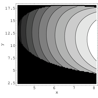
Figure 3: $\frac{1}{\Gamma}\frac{d\Gamma}{dx}$ spectrum for the $B^{-}\to K^{-}\phi\phi$ decay with the $\phi\phi$ invariant mass in the region below charm threshold and the Dalitz plot.

The distribution $(1/\Gamma)d\Gamma/dx$ as the function of the $\phi\phi$ invariant mass in the region below charm threshold and the Dalitz plot are is given in Fig. 2 for this case.

Note that the non-resonant contribution in the branching ratio, measured by Belle collaboration contains not only the non-resonant amplitude itself, but also the interference terms with the resonant contribution $B^{-}\to K^{-}\eta_{c}\to K^{-}\phi\phi$ as in [38]. In addition to the $\eta_{c}$ state there are a number of other $c\bar{c}$ bound states which might contribute. From these, the biggest contribution will arise from the $\chi_{c0}$ state as its mass is closest to the region we discuss ($x<2.85\,{\rm GeV}$). This contribution can be obtained from the measured $B^{-}\to\chi_{c0}K^{-}$ decay rate [39]. One might then expect that the $B^{-}\to\chi_{c0}K^{-}\to$ $\phi\phi K^{-}$ transition can give additional interference with the calculated rates. However, the rate for $\chi_{c0}\to\phi\phi$ is ten times smaller than the rate $\eta_{c}\to\phi\phi$ and we expect additional suppression. This leads us to the conclusion that the interference of the non-resonant and the resonant terms from the $c\bar{c}$ states other than $\eta_{c}$ is negligible below the charm threshold.

Next, we comment on the interference of the $\eta_{c}$ resonance with the non-resonant contribution in the region of the phase space with the invariant mass of the $\phi\phi$ state within the region $(2.94\,{\rm GeV})^{2}<x<(3.02\,{\rm GeV})^{2}$. The decay rate for $B^{-}\to K^{-}\eta_{c}$ is not theoretically very well understood. Naive factorization leads to a decay rate ten times smaller than the branching ratios $6.9^{+3.4}_{-3.0}\times 10^{-4}$ measured by CLEO collaboration [40], $(1.34\pm 0.09\pm 0.13\pm 0.41)\times 10^{-3}$ by BaBar collaboration [41] or $(1.25\pm 0.14^{+0.10}_{-0.12}\pm 0.38)\times 10^{-3}$ by Belle collaboration [42]. QCD factorization seems to face similar problem in explaining this decay amplitude [43]. On the other hand, the decay $\eta_{c}\to\phi\phi$ rate is not very well understood. First, the statistics for the $\eta_{c}\to\phi\phi$ decay rate is rather poor (the error stated in [21] seems to be underestimated [44]). Secondly, by assuming the SU(3) flavor symmetry one cannot reproduce both the $\eta_{c}\to\phi\phi$ and the $\eta_{c}\to\rho\rho$ measured decay rates.

Facing these difficulties we use experimental data to estimate the size of this resonant contribution. In the phase space region $(2.94\,{\rm GeV})^{2}<x<(3.02\,{\rm GeV})^{2}$, Belle measures ${\rm BR}(B^{-}\to K^{-}\eta_{c})\times{\rm BR}(\eta_{c}\to\phi\phi)=(2.2^{+1.0}_{-0.7}\pm 0.5)\times 10^{-6}$. We model ${\rm BR}(B^{-}\to K^{-}\eta,\eta^{\prime})\times{\rm BR}(\eta,\eta^{\prime}\to\phi\phi)$ by taking the $\eta_{c}$ propagator and by fitting the Belle’s data. The results for the interference are given on Fig. 3, where we present both cases: positive and negative interference terms, which is the result of an unknown phase in the $\eta_{c}\to\phi\phi$ decay amplitude.

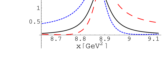
Figure 4: The $\frac{1}{\Gamma}\frac{d\Gamma}{dx}$ spectrum for $B^{-}\to K^{-}\phi\phi$ decay in $\eta_{c}$ resonance region. In full (black) line, we show only the resonant contribution while dotted (blue) and dashed (red) show the destructive and constructive interference with the non charm amplitude respectively.

The contribution of the $\eta_{c}$ resonance in the $x<(2.85\,{\rm GeV})^{2}$ region can affect the non-resonant branching ratio, reducing it to $3.3\times 10^{-6}$, in the case of destructive interference, or increasing it to $4.2\times 10^{-6}$ in the opposite case.

In the treatment of the decay $B^{-}\to\phi\phi K^{-}$ , due to the complexity of the problem, there are uncertainties which might be important. The simplest possible approach which will give us a reasonable estimate of the decay rates could be the use of factorization model for the weak vertices and the creation of the final state by the exchange of resonant states. Both assumptions bring in uncertainties themselves. The model should be tested when more experimental data on other $B$ decays into two vector and one pseudoscalar states will be available. The additional errors come from: the lack of understanding of the $B^{-}\to K^{-}\eta^{\prime}$ decay amplitude within the factorization approximation; the treatment of the two gluon exchange in the amplitudes of the $\eta K$, $\eta^{\prime}K$ modes [45] and the assumptions on $B^{-}\to\eta(1490)K^{-}$ decay mechanism. The other input parameters might introduce about $10\%$ uncertainty. Since the $\eta(1490)$ state gives important contribution to the rate, the theoretical ignorance of its coupling is potentially dangerous.

In conclusion, we have constructed a model, based on the naive factorization and the exchange of intermediate resonances, with the aim to understand the decay mechanism in the $B^{-}\to\phi\phi K^{-}$ decay with the $\phi\phi$ invariant mass in the region below charm threshold. We have found that the largest contribution in the rate comes from the decay chain $B^{-}\to\eta(\eta^{\prime},\eta(1490))K^{-}\to\phi\phi K^{-}$. Although this dominant contribution comes from the tree-level and penguin operators, we find that effects of the tree amplitudes are negligible. The interference effects of the $\eta_{c}$ resonance with the non-resonant contribution in the region of the phase space with the invariant mass of the $\phi\phi$ state in the region $(2.94\,{\rm GeV})^{2}<x<(3.02\,{\rm GeV})^{2}$ might decrease (or increase) the rate by $\sim 10\%$, depending on the sign of the interference term.

ACKNOWLEDGMENTS

We thank our colleagues P. Križan, B. Golob and T. Živko for stimulating discussions on experimental aspects of this investigation. The research of S. F. and A. P. was supported in part by the Ministry of Education, Science and Sport of the Republic of Slovenia.

References

[1] Belle Collaboration, H. C. Huang et al.,
Phys. Rev. Lett. 91, 241802 (2003) [hep-ex/0305068].
[2] H. Y. Cheng, K. C. Yang, Phys. Rev. D 66, 054015
(2002) [hep-ph/0205133].
[3] B. Bajc, S. Fajfer, R. J. Oakes, T.N. Pham,
S. Prelovšek, Phys. Lett. B 447, 313 (1999) [hep-ph/9809262].
[4] A. Ali, G. Kramer, C. D. Lu, Phys. Rev. D 58,
094009 (1998) [hep-ph/9804363].
[5] N. G. Deshpande, B. Dutta, S. Oh, Phys. Lett. B
473, 141 (2000) [hep-ph/9712445].
[6] L. N. Epele, D. G. Dumm, A. Szynkman,
Eur. Phys. J. C 29, 207 (2003) [hep-ph/0304070].
[7]
D. Du, H. Gong, J. Sun, D. Yang, G. Zhu,
Phys. Rev. D 65, 094025 (2002)
(Erratum-ibid: Phys. Rev. D 66, 079904 (2002)) [hep-ph/0201253];
M. Beneke, M. Neubert, Nucl. Phys. B 675, 333 (2003) [hep-ph/0308039].
[8]
C.W. Chiang, M. Gronau, Z. Luo, J. L. Rosner, D. A. Suprun,
hep-ph/0307395; C. W. Chiang, M. Gronau, J. L. Rosner,
Phys. Rev. D 68, 074012 (2003) [hep-ph/0306021].
[9] C. Dariescu, M. A. Dariescu, N. G.
Deshpande, D. K. Ghosh, hep-ph/0308305.
[10] V. V. Anisovich, D. I. Melikhov, V. A. Nikonov,
Phys. Rev. D 55, 2918 (1997);
[11] T. Feldmann, P. Kroll, Phys. Rev. D
58, 057501 (1998) [hep-ph/9805294]; T. Feldmann, P. Kroll, B. Stech,
Phys. Rev. D 58, 114006 (1998) [hep-ph/9802409].
[12] M. Beneke, M. Neubert, Nucl. Phys. B 651, 225
(2003) [hep-ph/0210085].
[13] A. Ali, G. Kramer, C. D. Lu, Phys. Rev. D 59,
014005 (1999) [hep-ph/9805403].
[14] A. Ali, C. Greub, Phys. Rev. D 57,
2996 (1998) [hep-ph/9707251].
[15] D. Becirevic, A. B. Kaidalov, Phys. Lett. B 478, 417 (2000)
[hep-ph/9904490]
[16] D. Melikhov, B. Stech, Phys. Rev. D 62, 014006
(2000) [hep-ph/0001113].
[17] S. Fajfer, R. J. Oakes, T. N. Pham, Phys. Lett. B,
539 67 (2002) [hep-ph/0203072].
[18] N. G. Deshpande, X. G. He, Phys. Lett. B 336,
471 (1994) [hep-ph/9403266]; N. G. Deshpande, X. G. He, W. S. Hou, S. Pakvasa,
Phys. Rev. Lett. 82, 2240 (1999) [hep-ph/9809329].
[19] C. Isola, T. N. Pham, Phys. Rev. D 62, 094002
(2000) [hep-ph/9911534].
[20] T. E. Browder, A. Datta, X. G. He, S. Pakvasa,
Phys. Rev. D 57, 6829 (1998) [hep-ph/9705320].
[21] Review of Particle Physics, Hagiwara et al.,
Phys. Rev D 66, 010001 (2002).
[22] D. Becirevič, “talk given at 2nd Workshop
on the CKM Unitarity Triangle, Durham, England, 5-9 April 2003”, hep-ph/0310072.
[23] M. Bando, T. Kugo, S. Uehara, K. Yamawaki,
T. Yanagida, Phys. Rev. Lett. 54, 1215 (1985); M. Bando,
T. Kugo, K. Yamawaki, Nucl. Phys. B 259, 493 (1985);
M. Bando, T. Kugo, K. Yamawaki, Phys. Rept. 164, 217 (1988).
[24] T. Fujiwara, T. Kugo, H. Terao, S. Uehara,
K. Yamawaki, Prog. Theor. Phys. 73, 926 (1985).
[25] A. Bramon, A. Grau, G. Pancheri, Phys. Lett. B 344, 240 (1995).
[26] S. Fajfer, P. Singer, Phys. Rev. D 56, 4302
(1997).
[27] H. C. Huang (for Belle Collaboration), “presented at the
Recontres de Moriond on Electroweak Interactions and Unified Theories,
Les Arcs, France, 9-16 March 200”, hep-ex/0205062.
[28] Belle Collaboration, K. F. Chen et al., Phys. Rev Lett 91, 201801
(2003) [hep-ex/0307014].
[29] BaBar Collaboration, B. Aubert et al., “presented at the
Recontres de Moriond on QCD and Hadronic Interactions, Les Arcs, France, 22-29 March 2003”,
hep-ex/0303039.
[30] BaBar Collaboration, B. Aubert et al., Phys. Rev. Lett 91, 161801
(2003) [hep-ex/0303046].
[31] BaBar Collaboration, B. Aubert et al., “presented at the
Recontres de Moriond on Electroweak Interactions and Unified Theories,
Les Arcs, France, 15-22 March 2003”, hep-ex/0303029.
[32] BaBar Collaboration, B. Aubert et al., Phys. Rev Lett 91, 171802 (2003)
[hep-ex/0307026].
[33] J. R. Fry, talk given at Lepton Photon Conference,
Fermilab, 2003.
[34] C. S. Kim, B. H. Lim, S. Oh, Eur. Phys. J. C 22, 683
(2002).
[35] C. S. Kim, J. P. Lee, S. Oh, Phys. Rev. D 67, 014002
(2003).
[36] N. R. Stanton et al., Phys. Rev. Lett. 42,346 (1979);
A. V. Anisovich, V. V. Anisovich, V. A. Nikonov, Eur. Phys. J. A6, 247 (1999) [hep-ph/9910321].
[37] W. S. Carvalho, A. C. B. Antunes, A. S. de Cstro,
Eur. Phys. J. C 7, 95 (1999).
(2002).
[38] B. Bajc, S. Fajfer, R. J. Oakes, T. N. Pham,
Phys. Rev. D 58, 054009 (1998) [hep-ph/9710422].
[39] Belle Collaboration, K. Abe et al.,
Phys. Rev. Lett. 88, 031802 (2002) [hep-ph/0111069],
BaBar Collaboration, B. Aubert et al., hep-ex/0310015.
[40]
CLEO Collaboration, K. W. Edwards et al., Phys. Rev. Lett.
86, 30 (2001).
[41] BaBar Collaboration, B. Aubert et al., hep-ex/0403007.
[42] Belle Collaboration, F. Fang et al., Phys. Rev. Lett 90,
071801 (2003) [hep-ex/0208047].
[43]
Z. Song, C. Meng, K-T. Chao, hep-ph/0209257.
[44]
Argus Collaboration,
H. Albercht et al., Phys. Lett B 338,390 (1994).
[45] see for example J. O. Eeg, K. Kumericki, I. Picek, Phys. Lett B 563, 87
(2003) [hep-ph/0304274].