Evidence for Factorization in Three-body $\overline{B}\to D^{(*)}\,K^{-}\,K^{0}$ Decays

Abstract

Motivated by experimental results on $\overline{B}\to D^{(*)}K^{-}K^{0}$, we use a factorization approach to study these decays. Two mechanisms concerning kaon pair production arise: current-produced (from vacuum) and transition (from the $B$ meson). The kaon pair in the $\overline{B}{}^{0}\to D^{(*)+}K^{-}K^{0}$ decays can be produced only by the vector current (current-produced), whose matrix element can be extracted from $e^{+}e^{-}\to K\overline{K}$ processes via isospin relations. The decay rates obtained this way are in good agreement with experiment. The $B^{-}\to D^{(*)0}K^{-}K^{0}$ decays involve both current-produced and transition processes. By using QCD counting rules and the measured $B^{-}\to D^{(*)0}K^{-}K^{0}$ decay rates, the measured decay spectra can be understood.

1 Introduction

The $\overline{B}\to D^{(*)}K^{-}K^{(*)0}$ decays have been observed for the first time by the Belle Collaboration Drutskoy:2002ib , with branching fractions at the level of $10^{-4}-10^{-3}$. Angular analysis reveals that $K^{-}K^{0}$ and $K^{-}K^{*0}$ are dominantly $J^{P}=1^{-}$ and $1^{+}$, respectively. While there is no sign of decay via resonance for the $K^{-}K^{0}$ pair, data suggest a dominant $a_{1}(1260)$ resonance contribution in the production of the $K^{-}K^{*0}$. The $K^{-}K^{(*)0}$ mass spectra are peaking near threshold.

The near-threshold peaking of the $K^{-}K^{(*)0}$ mass spectra suggests a quasi two-body process where the colinear $K^{-}K^{(*)0}$ recoil against the $D^{(*)}$ meson. This is suggestive to apply fatorization to the three-body case Chua:2002pi . Two kinds of decay amplitudes arise due to the flavor structures of the $D^{(*)}$ mesons: $D^{(*)+}K^{-}K^{(*)0}$ involves $\langle K^{-}K^{(*)0}|V-A|0\rangle$, with $K^{-}K^{(*)0}$ produced by a weak $V-A$ current; $D^{(*)0}K^{-}K^{(*)0}$ involves $\langle K^{-}K^{(*)0}|V-A|B^{-}\rangle$, where $B^{-}$ goes into $K^{-}K^{(*)0}$ via a weak current.

In $\langle K^{-}K^{0}|V-A|0\rangle$, the $K^{-}K^{0}$ can only be produced by the vector current, and should be dominantly $1^{-}$. By isospin rotation, the kaon weak form factor $\langle K^{-}K^{0}|V|0\rangle$ can therefore be related to the kaon electromagnetic (EM) form factors in $e^{+}e^{-}$ annihilation, where much data exist. One can then calculate the rate without any tuning parameters. The predicted $K^{-}K^{0}$ mass spectrum can be shown to have a peak near threshold, which arises from the kaon form factor and can be checked by experiment.

In $B^{-}\to D^{(*)0}K^{-}K^{0}$ decays, the $K^{-}K^{0}$ can also be produced by a current that induces $B^{-}\to K^{-}K^{0}$ transitions. The relevant matrix element $\langle K^{-}K^{0}|V-A|B^{-}\rangle$ is parameterized by several unknown form factors, due to which the rate cannot be calculated. Nevertheless, by using a naive parametrization based on QCD counting rules Brodsky:1974vy , the parameters in these unknown form factors can be determined from the decay rates, and the decay spectra can be obtained, which again have threshold enhancement as closely related to QCD counting rules, and can be tested experimentally.

The $K^{-}K^{*0}$ in $\overline{B}{}^{0}\to D^{(*)+}K^{-}K^{*0}$ can only be produced by a weak current. The experimental observation that $K^{-}K^{*0}$ is in $1^{+}$ suggests a dominant axial current contribution. Although the decay rate cannot be calculated due to the absence of data of the $K^{-}K^{*0}$ axial form factors, it has been proposed that one can extract the $K^{-}K^{*0}$ axial form factors given the $K^{-}K^{*0}$ mass spectrum DKKstar .

In what follows, we shall concentrate on decays that involve only $K^{-}K^{0}$. In the next section we will introduce the relevant formalism and describe the numerical results. A discussion will be given in the last section where the conclusion is drawn.

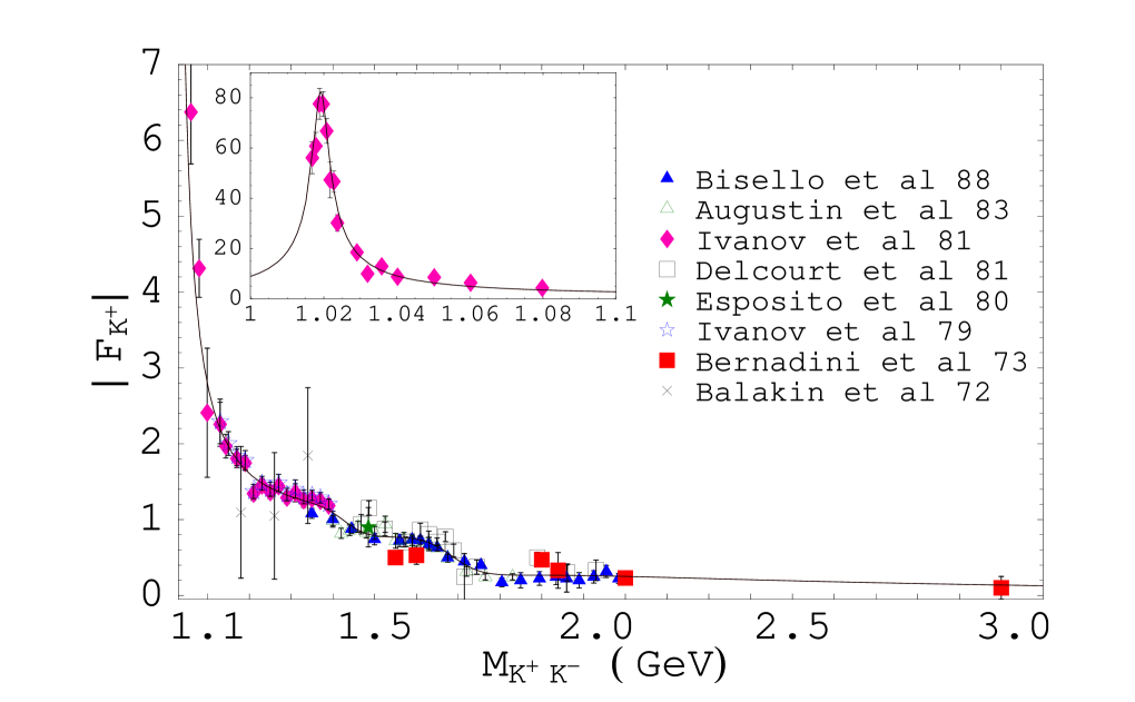
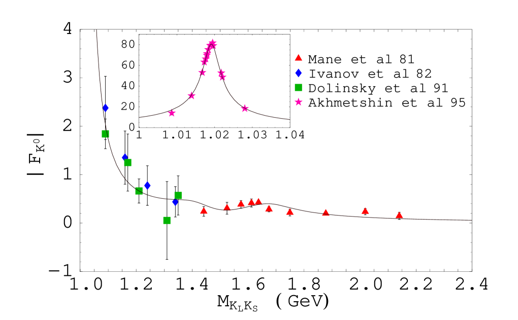
Figure 1: Fit to timelike $|F_{K^{+}}|$ (upper) and $|F_{K^{0}}|$ (lower) form factor data, where the inset is for the $\phi$ region.

2 Factorization Formalism

Starting with the relevant effective Hamiltonian, and the factorization ansatz, one arrives at Chua:2002pi

$${\mathcal{A}}(D^{(*)+}K^{-}K^{(*)0}) = \frac{G_{F}}{\sqrt{2}}V_{cb}V_{ud}^{*}\,a_{1}\langle D^{(*)+}|(\bar{c}b)_{V-A}|\overline{B}{}^{0}\rangle$$ (1)

$$\times\langle K^{-}K^{(*)0}|(\bar{d}u)_{V}|0\rangle,$$

$${\mathcal{A}}(D^{(*)0}K^{-}K^{(*)0}) = \frac{G_{F}}{\sqrt{2}}V_{cb}V_{ud}^{*}\big{[}a_{1}\langle D^{(*)0}|(\bar{c}b)_{V-A}|B^{-}\rangle$$ (2)

$$\times\langle K^{-}K^{(*)0}|(\bar{d}u)_{V}|0\rangle$$

$$+a_{2}\langle K^{-}K^{(*)0}|(\bar{d}b)_{V-A}|B^{-}\rangle$$

$$\times\langle D^{(*)0}|(\bar{c}u)_{V-A}|0\rangle\big{]},$$

in which

$$\langle K^{-}(p_{K^{-}})K^{0}(p_{K^{0}})\left|V^{\mu}\right|0\rangle=(p_{K^{-}}-p_{K^{0}})^{\mu}F_{1}^{KK}(q^{2})$$ (3)

in the isospin limit, and

$$\langle K^{-}(p_{K^{-}})K^{0}(p_{K^{0}})|(V-A)_{\mu}|B^{-}(p_{B})\rangle$$

$$\qquad=iw_{-}(q^{2})(p_{K^{-}}-p_{K^{0}})_{\mu}$$

$$\qquad\quad+\,h(q^{2})\,\epsilon_{\mu\nu\alpha\beta}\,p_{B}^{\nu}q^{\alpha}(p_{K^{-}}-p_{K^{0}})^{\beta},$$ (4)

where $q\equiv p_{K^{-}}+p_{K^{0}}$. The fact that $K^{-}K^{0}$ is in $1^{-}$ has been taken into account in the above parametrizations. The $\langle D^{(*)}|(\bar{c}b)_{V-A}|\overline{B}\rangle$ is the same as in two-body cases and we adopt both the BSW BSW:physC29 and the MS Melikhov:2000yu models for comparison.

The kaon weak vector form factor $F^{KK}_{1}$ is related to its EM partners via the isospin relation

$$F^{KK}_{1}(q^{2})=F_{K^{+}}(q^{2})-F_{K^{0}}(q^{2}),$$ (5)

where $F_{K^{+}}$, $F_{K^{0}}$ are the EM form factors of the charged and neutral kaons, respectively. By fitting to the EM data, one can obtain the kaon EM form factors and hence the weak vector form factor Chua:2002pi , as shown in Figs. 1 and 2. Readers are referred to Chua:2002pi for detailed discussion on the fitting of kaon EM form factors.

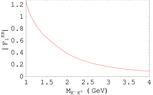
Figure 2: The kaon weak vector form factor $F^{KK}_{1}$.

For the unknown form factors in Eq. 4, we take the following naive parametrization Chua:2002pi

$$w_{-}(t)=\frac{c_{w}}{t^{2}},\qquad h(t)=\frac{c_{h}}{t^{2}},$$ (6)

where $c_{w,h}$ are free parameters to be fitted by data. The $1/t^{2}$ arises from the minimum number of hard gluons to produce an energetic kaon pair from a decaying $B$ meson, which characterizes the asymptotic behavior of the form factor.

Table 1: ${\cal B}(\overline{B}^{0}\to D^{(*)+}K^{-}K^{0})$ in units of $10^{-4}$.

	MS	BSW	Experiment Drutskoy:2002ib
$\overline{B}{}^{0}\to D^{+}K^{-}K^{0}$	$1.67^{+0.24}_{-0.21}$	$1.54^{+0.22}_{-0.20}$	$1.6\pm 0.8\pm 0.3$
			$<3.1$ ($90\%$ CL)
$\overline{B}{}^{0}\to D^{*+}K^{-}K^{0}$	$2.8^{+0.30}_{-0.36}$	$3.05^{+0.32}_{-0.39}$	$2.0\pm 1.5\pm 0.4$
			$<4.7$ ($90\%$ CL)

In Table 1 we show the calculated branching fractions of the $\overline{B}{}^{0}\to D^{(*)+}K^{-}K^{0}$ modes. One can see that the results are in very good agreement with experiment. In the absence of any tuning parameters in our formalism for these decay modes, the agreement between experiment and the model actually provides evidence for factorization!

On the other hand, the predicted $K^{-}K^{0}$ mass spectra in Fig. 3 of the $D^{(*)+}K^{-}K^{0}$ modes show peaks close to threshold, which is due to the near-threshold behavior of the $F^{KK}_{1}$ form factor (see Fig. 2). There is no other clear structure, other than the $B\to D^{*}$ form factor effect at larger $q^{2}$. Because of lower $D^{(*)+}$ reconstruction efficiencies, the spectra has yet to be measured experimentally Drutskoy:2002ib , but our predicted spectrum can be checked soon with more data.

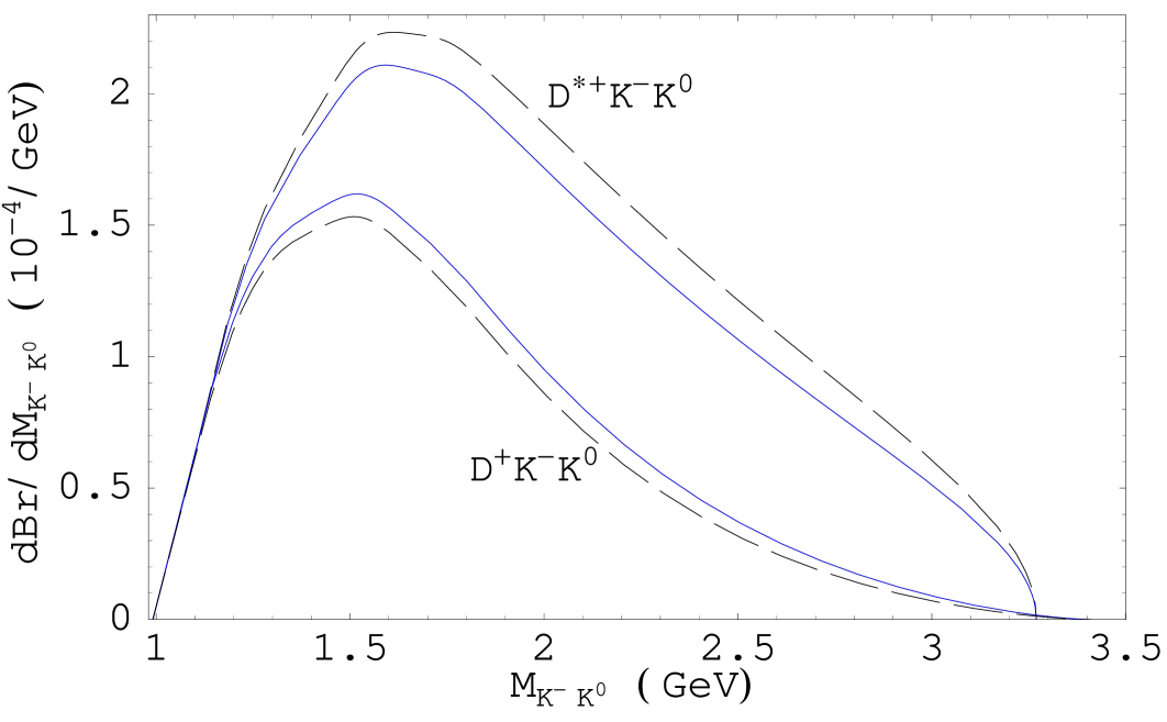
Figure 3: The $K^{-}K^{0}$ mass spectrum for $\overline{B}{}^{0}\to D^{+}K^{-}K^{0}$ (lower) and $D^{*+}K^{-}K^{0}$ (upper), where solid (dashed) line stands for using the MS (BSW) hadronic form factors.

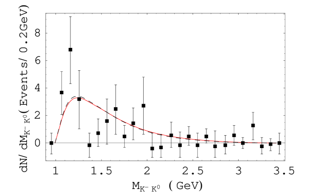
Figure 4: $B^{-}\to D^{0}K^{-}K^{0}$ spectrum, where solid (dashed) line is for the MS (BSW) model, and the data is from Ref. Drutskoy:2002ib .

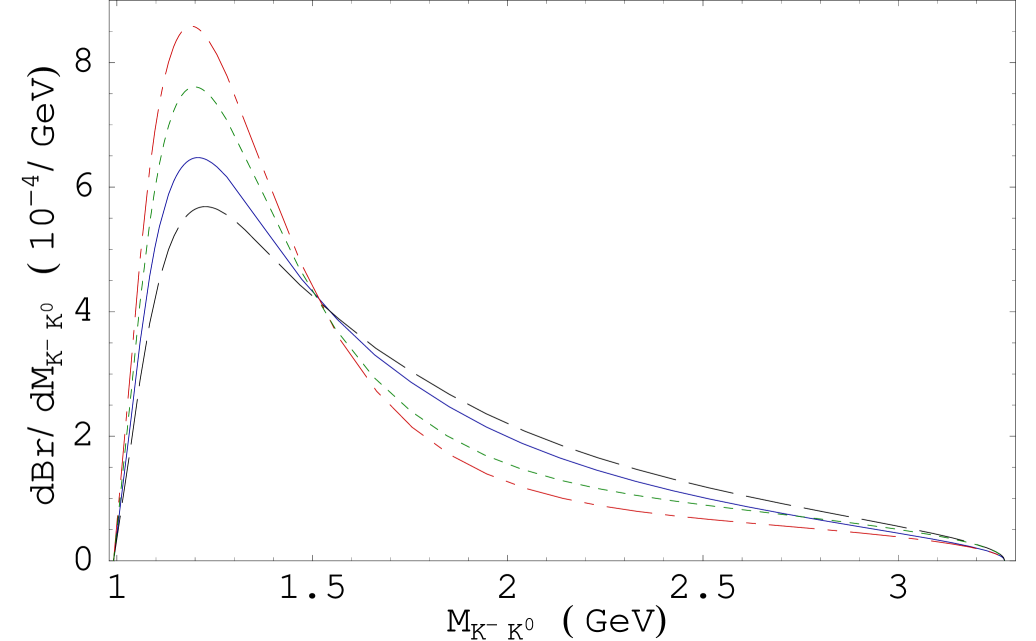
Figure 5: The $K^{-}K^{0}$ mass spectrum for $B^{-}\to D^{*0}K^{-}K^{0}$, where solid, dot-dashed, dashed and dotted lines are for MS model with $c_{h}=11.3,\ -16.1$ GeV³ and BSW model with $c_{h}=13.1,\ -18.5$ GeV³, respectively.

For $B^{-}\to D^{(*)0}K^{-}K^{0}$ which involve the unknown parameters $c_{w_{-}}$, $c_{h}$, we fit to the decay rates to obtain their values, as shown in Table 2. The $K^{-}K^{0}$ mass spectra can then be obtained, in particular for the $B^{-}\to D^{0}K^{-}K^{0}$ mode, where one can see from Fig. 4 that the $K^{-}K^{0}$ mass spectrum can be roughly described by the naive form factor model of Eq. 6. The mass spectrum of $B^{-}\to D^{*0}K^{-}K^{0}$ in Fig. 5 can be checked in experiment.

Table 2: Fitted values of transition form factor parameters $c_{w_{-}}$ and $c_{h}$, by using the central values of $D^{(*)0}K^{-}K^{0}$ rates. See Chua:2002pi for detailed discussions.

	$c_{w_{-}}^{\rm MS(BSW)}$ (GeV3)	$c_{h}^{\rm MS(BSW)}$ (GeV3)	${\mathcal{B}}(10^{-4})$ Drutskoy:2002ib
$B^{-}\to D^{0}K^{-}K^{0}$	$-35.4~{}(-33.0)$	—	$5.5\pm 1.4\pm 0.8$
$B^{-}\to D^{*0}K^{-}K^{0}$	$-35.4~{}(-33.6)$	$11.3~{}(13.1)$ or $-16.1~{}(-18.5)$	$5.2\pm 2.7\pm 1.2$

3 Discussion and Conclusion

A factorization approach has been used to study three-body $\overline{B}\to D^{(*)}K^{-}K^{0}$ decays. There are two mechanisms of kaon pair production, namely current-produced and transition. For $\overline{B}^{0}\to D^{(*)+}K^{-}K^{0}$ which involve the former, one can make use of kaon EM data through isospin rotations. The result is in good agreement with experiment, which supports factorization.

The $B^{-}\to D^{(*)0}K^{-}K^{0}$ decays also receive the transition contribution. The form of these transition form factors are determined through QCD counting rules, and we fix the parameters by using the measured $D^{0}K^{-}K^{0}$ and $D^{*0}K^{-}K^{0}$ decay rates. The predicted mass spectra of the $B^{-}\to D^{0}K^{-}K^{0}$ mode agrees well with data and exhibit threshold enhancement as do the $\overline{B}{}^{0}\to D^{(*)+}K^{-}K^{0}$ cases. Despite the success in describing the mass spectrum of the $D^{0}K^{-}K^{0}$ mode, our treatment of the $B^{-}\to K^{-}K^{0}$ transition form factors may be oversimplified. Assuming the asymptotic form required by PQCD may be too strong an assumption, and might have over-enhanced the contribution from the near-threshold region. More careful study on other possibilities, such as using pole models for transition via resonances, would be helpful in clarifying the underlying dynamics of the $B^{-}\to D^{(*)0}K^{-}K^{0}$ transitions.

Finally, with the feasibility of extracting $K^{-}K^{*0}$ axial form factors emboldened by the success in $\overline{B}\to D^{(*)}K^{-}K^{0}$ decays, $B$ decay data plus factorization have opened up a new avenue to the study of meson form factors, which have traditionally been fundamental quantities to many fields in both nuclear and elementary particle physics. The success of factorization in $\overline{B}\to D^{(*)}K^{-}K^{0}$ decays urges a serious study of the underlying mechanism.

References

(1)
A. Drutskoy et al. [Belle Collaboration],
Phys. Lett. B 542, (2002) 171 [arXiv:hep-ex/0207041].
(2)
C. K. Chua, W. S. Hou, S. Y. Shiau and S. Y. Tsai,
Phys. Rev. D 67, (2003) 034012 [arXiv:hep-ph/0209164].
(3)
S. J. Brodsky and G. R. Farrar,
Phys. Rev. D 11, (1975) 1309.
(4)
C. K. Chua, W. S. Hou, S. Y. Shiau and S. Y. Tsai, in preparation.
(5)
M. Wirbel, B. Stech and M. Bauer,
Z. Phys. C 29, (1985) 637.
(6)
D. Melikhov and B. Stech,
Phys. Rev. D 62, (2000) 014006 [arXiv:hep-ph/0001113].