CERN-PH-TH/2004-003 IFT-02-04 UCD-04-14

Low-energy effective theory from
a non-trivial scalar background in extra dimensions

ABSTRACT

Consequences of a non-trivial scalar field background for an effective 4D theory were studied in the context of one compact extra dimension. The periodic background that appears within the (1+4)-dimensional $\phi^{4}$ theory was found and the excitations above the background (and their spectrum) were determined analytically. It was shown that the presence of the non-trivial solution leads to the existence of a minimal size of the extra dimension that is determined by the mass parameter of the scalar potential. It was proved that imposing orbifold antisymmetry boundary conditions allows us to eliminate a negative mass squared Kaluza–Klein ground-state mode that otherwise would cause an instability of the system. The localization of fermionic modes in the presence of the non-trivial background was discussed in great detail varying the size of the extra dimension and the strength of the Yukawa coupling. A simple exact solution for the zero-mode fermionic states was found and the solution for non-zero modes in terms of trigonometric series was constructed. The fermionic mass spectrum, which reveals a very interesting structure, was found numerically. It was shown that the natural size of the extra dimension is twice as large as the period of the scalar background solution.

PACS: 11.10.Kk, 11.27.+d

Keywords: anomalous extra dimensions, kink solutions, fermion localization

1 Introduction

A typical habit, which has its roots in the (1+3)-dimensional Standard Model (SM) and its possible 4D alternatives, is to assume that the Higgs boson (or any other scalar) vacuum expectation value (vev) has a constant value. In 4D theories, this is a consequence of the requirement of the 4D translational invariance. However, in models of the electroweak interactions built upon $1+(3+d)$-dimensional manifolds, the translation invariance is no longer required, as the extra dimensions must be compact. Here we will consider the space-time manifold that is $M^{(3,1)}\times R$, where $M^{(3,1)}$ is the usual Minkowski space, while $R$ is a compact manifold. The vev is no longer forced to be a constant by the (4D) symmetries that are typically imposed, and therefore it can have a non-trivial profile along the extra direction: $\langle\phi(x,y)\rangle=\phi_{c}(y)$, where $x$ is in an element of $M^{(3,1)}$ Minkowski space-time, while $y$ is the extra coordinate (hereafter we will restrict ourselves to $R=S^{1}/Z_{2}$). Recently, it has been noticed [1, 2] that the non-trivial $y$-dependence of the vev of a scalar field could be very useful phenomenologically, since it may lead to a natural localization of higher-dimensional fermions on lower-dimensional manifolds (“fat brane scenario”). This is a very attractive approach, since it allows us to control the effective couplings between 4D states by tuning the overlap of their wave function in the extra dimension [4, 5]. In fact a similar idea had already been explored in the mid-seventies, in the context of domain walls that separate regions of different vacuum expectation values of a scalar field [6], see also [7].

The standard approximation adopted in the studies of non-trivial scalar vev’s in extended compact space-times was to assume that the size of the extra dimension $L$ is much larger than the typical scale of the scalar field potential $m$. In this paper we will show how to construct a low-energy effective theory exactly, including the determination of the Kaluza–Klein (KK) states of scalars and fermions and their mass spectrum, in the case of a scalar with a Higgs-like potential in 5D.

First we will consider a 5D model of a free real scalar field $\phi=\phi(x,y)$ defined by the following Lagrangian density:

$${\cal L}^{(5)}=\frac{1}{2}\;\partial^{M}\phi(x,y)\;\partial_{M}\phi(x,y)-V^{(5)}(\phi)$$ (1)

with $y\equiv x^{4}$ and

$$V^{(5)}(\phi)={\lambda\over 4}\left(|\phi|^{2}-{m^{2}\over\lambda}\right)^{2}\,.$$ (2)

Below we will look for a field configuration $\phi_{c}(x,y)$ that corresponds to the extrema of the classical action. Since the fifth dimension is compact we will allow for a non-trivial dependence of the background solution on the extra coordinate. In addition, we will restrict ourselves to time-independent solutions, so $\phi_{c}=\phi_{c}(y)$.

After a single integration of the Euler–Lagrange equation:

$$\partial_{M}\partial^{M}\phi+{\partial V^{(5)}\over\partial\phi}=0$$ (3)

we obtain the following equation for the background $\phi_{c}$ that describes the energy conservation of the system:

$$\frac{1}{2}\phi_{c}^{{}^{\prime}\;2}-V(\phi_{c})=E={\rm const.}\,,$$ (4)

where ${}^{{}^{\prime}}$ denotes a differentiation with respect to $y$. It is seen that our field theoretical problem corresponds to a 1D motion of the classical material point in the potential $-V(\phi_{c})$, where $\phi_{c}$ is the coordinate, $y$ corresponds to the time and $E$ is interpreted as the total energy. It is easy to see that for $E=0$ we obtain a non-trivial solution of (4) known as the kink and antikink:

$$\phi_{c}^{\rm kink}(y;y_{0})=\pm{m\over\sqrt{\lambda}}\tanh\left[{m\over\sqrt{2}}(y-y_{0})\right]$$ (5)

where the constant $y_{0}$ is the “kink-location”. The kink solution corresponds to the motion of the point, starting with zero velocity at the top of one of the hills of the potential $-V(\phi_{c})$ (located at $\phi_{c}=\pm m/\sqrt{\lambda}$) and moving down toward the origin, and then, after an infinite amount of “time” ($y$), reaching the next hill. The above solution assumes that the integration constant $E$ of Eq. (4) is zero. It is easy to argue that this is really a necessary choice for a non-compact space, however in our case of the compact fifth dimension there is no reason to assume $E=0$. From the mechanical analogy it is also seen that if the material point starts at $y$, it will then move toward the origin and eventually, after a finite time, reach the symmetric position at $-y$. Obviously the point then returns, so that the motion will be periodic.

The paper is organized as follows. In Sec. 2 we will find a periodic kink-like solution for the scalar background. The KK modes and their corresponding masses for the free scalar considered will be determined there. In section 3 we will add a fermion field coupled to the scalar. We will show how to solve the Schrödinger-like equation for all the fermionic modes and their corresponding masses, and in this way we find states not considered until now, which have very interesting implications, both phenomenologically and in model building. We then summarize our results in the final Section 4.

2 Periodic Kink-Like Background Profile

It is straightforward to integrate Eq. (4) even for $E\neq 0$:

$$y-y_{0}=\pm{1\over m}\int{d\varphi\over\sqrt{\varphi^{4}-\varphi^{2}+{c\over 2}}}\,,$$ (6)

where $y_{0}$ and $E$ are constants of integration and we have defined the dimensionless parameter $c={1\over 2}+{2E\lambda\over m^{4}}$, and the field has been rescaled as follows: $\varphi=\lambda/(2m^{2})\phi_{c}$.

We are interested in solutions $\phi_{c}(y)$ (or $\varphi(y)$), which are periodic and continuous. It is easy to see from the mechanical model that this can only happen when $0<c<1/2$. In that case the background solution is bounded by $|\phi_{c}(y)|\leq{m\over\sqrt{\lambda}}$ and is given by

$$\phi_{c}(y)=\pm{m\over\sqrt{\lambda}}\sqrt{2k^{2}\over k^{2}+1}\ {\rm sn}\left({m(y-y_{0})\over\sqrt{k^{2}+1}},\ k^{2}\right)$$ (7)

where

$$k^{2}={1-\sqrt{1-2c}\over c}-1={m^{2}-2\sqrt{|\lambda E|}\over m^{2}+2\sqrt{|\lambda E|}}$$ (8)

and ${\rm sn}(x,k^{2})$ is the Jacobi elliptic-sine amplitude of modulus $k$ [12]. These solutions are parametrized by the modulus $k$, and since $0<c<1/2$, we have $0<k<1$. The function ${\rm sn}(x,k^{2})$ is odd in $x$, and oscillates between $1$ and $-1$. Its period is $4K$ where

$$K(k^{2})=\int_{0}^{\pi/2}{d\theta\over(1-k^{2}\sin^{2}\theta)}=F\left({\pi\over 2},k\right)$$ (9)

is the complete elliptic integral of the first kind [12]. The modulus $k$ depends on the constant $c$, which in turn depends on $E$, and therefore it is a free parameter that will determine the size of the extra dimension $L$ through the value of the period $\omega=4\sqrt{k^{2}+1}K(k^{2})/m$ . We see that the size of the extra dimension is not fixed by any dynamics, and therefore an unknown stabilization mechanism must be assumed.

In Fig. 1 we show the profile of the non-trivial background $\phi_{c}(y)$ for different values of $k^{2}$ (i.e. for different compactification scales). We also show the energy density $\epsilon(y)$

$$\epsilon(y)={1\over 2}(\partial_{y}\phi_{c})^{2}+V(\phi_{c})\,.$$ (10)

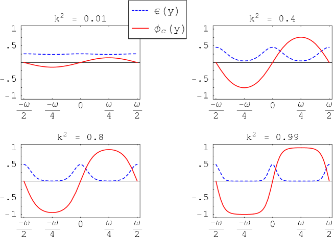
Figure 1: The profiles of the non-trivial background $\phi_{c}(y)$ (in units of $m/\sqrt{\lambda}$) and the “energy density” $\epsilon(y)$ (in units of $m^{4}/\lambda$) for $k^{2}=0.01,\ 0.4,\ 0.8$ and $0.99$ (or $\omega=1.01\omega_{0},\ 1.34\omega_{0},\ 1.93\omega_{0}$ and $3.32\omega_{0}$, with $\omega_{0}=2\pi/m$). We have chosen $y_{0}=0$; for $y_{0}\neq 0$, $y$ should be replaced by $y+y_{0}$.

We can now look at two interesting limits:

• $k\to 0$, then $\phi_{c}(y)\to\pm{m\over\sqrt{\lambda}}\sqrt{2}k\ \sin{m(y-y_{0})}+{\cal O}(k^{2})\ \ \to 0$. The background thus vanishes in the limit.

• $k\to 1$, then $\phi_{c}(y)\to\pm{m\over\sqrt{\lambda}}\tanh{m\sqrt{1\over 2}\ (y-y_{0})}$. Note that in this limit the periodicity of the background is being lost, even though $\phi_{c}(y)$ is a perfectly periodic function for any $k<1$.

The first limit corresponds to $c\to 0$. In this case although the non-trivial profile vanishes, there is a limiting period $\omega_{0}\equiv\omega\left.\right|_{k=0}=4K(0)/m=2\pi/m$. This means that there is a minimum size for the extra dimension, which is fixed by the mass parameter $m$ of the potential. This is easy to understand by recalling our mechanical analogue of the field theoretical problem. Namely, the limit $k\to 0$ ($c\to 0$) corresponds to the total energy $E\to-m^{4}/(4\lambda)$ that is the bottom of the classical potential ($-V(h)$). In that region, since the quartic part of the potential could be neglected, we observe small harmonic oscillations around the minimum $y=0$ . There thus exists a minimal period that is fixed to be $2\pi/m$ by the quadratic term (the mass term) of the potential. Consequently, if the scalar background is non-trivial, then there is a minimal size of the extra dimension that is a multiple of $\omega_{0}$. Note that we did not to impose the periodicity; whenever $0<k<1$ the solution must be periodic for any parameter of the model, no fine-tuning is needed.

The second limit, $k\to 1$ ($c\to 1/2$) corresponds to $E\to 0$, i.e. the motion that starts exactly at the top of a hill of the classical potential ($-V(h)$). In this case the total available time ($y$) needed to reach the other summit is infinite and therefore so is the corresponding size of the extra dimension $L$.

2.1 Scalar spectrum

$n$	$\phi_{n}$	$\frac{M_{n}^{2}}{m^{2}}$	$\left.\phi_{n}\right|_{k^{2}=1}$	$\left.\frac{M_{n}^{2}}{m^{2}}\right|_{k^{2}=1}$	$\left.\frac{M_{n}^{2}}{m^{2}}\right|_{k^{2}=0}$	Period
$0^{++}$	${\rm sn}^{2}(s,k^{2})-{1+k^{2}+\sqrt{1-k^{2}+k^{4}}\over 3k^{2}}$	$1-\sqrt{1+3({1-k^{2}\over 1+k^{2}})^{2}}$	${\rm tanh}^{2}(s)-1$	$0$	$-1$	$\omega^{\prime}/2$
$0^{+-}$	${\rm cn}(s,k^{2})\ {\rm dn}(s,k^{2})$	0	${\rm sech}^{2}(s)$	$0$	$0$	$\omega^{\prime}$
$1^{-+}\$	${\rm sn}(s,k^{2})\ {\rm dn}(s,k^{2})$	${3k^{2}\over 1+k^{2}}$	${\rm sech}(s)\ {\rm tanh}(s)$	$\frac{3}{2}$	$0$	$\omega^{\prime}$
$1^{--}$	${\rm sn}(s,k^{2})\ {\rm cn}(s,k^{2})$	${3\over 1+k^{2}}$	${\rm sech}(s)\ {\rm tanh}(s)$	$\frac{3}{2}$	$3$	$\omega^{\prime}/2$
$2^{++}\$	${\rm sn}^{2}(s,k^{2})-{1+k^{2}-\sqrt{1-k^{2}+k^{4}}\over 3k^{2}}$	$1+\sqrt{1+3({1-k^{2}\over 1+k^{2}})^{2}}$	${\rm tanh}^{2}(s)-\frac{1}{3}$	2	$3$	$\omega^{\prime}/2$

Table 1: The first five unnormalized scalar eigenfunctions and the resulting mass spectrum from Eq. (15). Here, $\omega^{\prime}=4K(k^{2})$ is the “rescaled” period of the background solution $\phi_{c}(s)$. The parities are defined with respect to $s=0$ and $s=\omega^{\prime}/4$.

Let us now expand the Lagrangian (1) around the background (7):

$$\phi(x,y)\to\phi_{c}(y)+\phi(x,y)\,,$$ (11)

where $\phi(x,y)$ that appears on the right-hand side of $\to$ is a fluctuation. Let us separate contributions to the Lagrangian density that are quadratic in the fluctuations $\phi(x,y)$:

$${\cal L}(x,y)=\frac{1}{2}\partial_{\mu}\phi\partial^{\mu}\phi-\frac{1}{2}\;\phi\left[-{d^{2}\over dy^{2}}+\left.{\partial^{2}V^{(5)}\over\partial\phi^{2}}\right|_{\phi=\phi_{c}}\right]\phi+\cdots\,,$$ (12)

where I have integrated by parts and dropped the total derivative because of periodicity. Let us expand in terms of the KK modes that are defined in such a way that the mass matrix is diagonal:

$$\left[-{d^{2}\over dy^{2}}+\left.{\partial^{2}V^{(5)}\over\partial\phi^{2}}\right|_{\phi=\phi_{c}}\right]\phi_{n}(y)=M_{n}^{2}\phi_{n}(y),$$ (13)

where the expansion $\phi(x,y)=\sum\phi_{n}(y)\chi_{n}(x)$ was adopted, and $M_{n}$ denote diagonal masses of the KK modes $\chi_{n}(x)$.

Substituting the background $\phi_{c}(y)$ from Eq. (7) we obtain the following equation to determine the right KK basis:

$$-\phi_{n}^{\prime\prime}(y)+\left[6m^{2}{k^{2}\over k^{2}+1}{\rm sn}^{2}\left(m\sqrt{1\over k^{2}+1}\ (y-y_{0}),\ k^{2}\right)-m^{2}-M_{n}^{2}\right]\ \phi_{n}(y)=0$$ (14)

By a suitable rescaling, $s={m\over\sqrt{k^{2}+1}}\ (y-y_{0})$ we can get

$$\phi_{n}^{\prime\prime}(s)+\left[(k^{2}+1)(1+{M_{n}^{2}\over m^{2}})-6k^{2}{\rm sn}^{2}\!\left(s,\ k^{2}\right)\right]\ \phi_{n}(s)=0\,,$$ (15)

which is the Lamé equation (in the Jacobian form)

$$\phi_{n}^{\prime\prime}(s)+\left[h-n(n+1)k^{2}{\rm sn}^{2}\!\left(s,\ k^{2}\right)\right]\ \phi_{n}(s)=0\,,$$ (16)

where $n=2$ and $h=(k^{2}+1)(1+{M_{n}^{2}\over m^{2}})$. It is known that for given $n$ and $k$, periodic solutions of the Lamé equation exist for an infinite sequence of characteristic values of $h$ [12]. Moreover, the periodic solutions will be of period $2K(k^{2})$ and $4K(k^{2})$, where $2K(k^{2})$ is the period of the Lamé equation (16).

Each of these characteristic values of $h$ will determine the KK mass of the corresponding mode. In the case that $n$ in (16) is integer, the first $2n+1$ solutions will be polynomials in the Jacobi elliptic functions. For the case $n=2$ at hand, the first 5 eigenmodes are simple enough [9, 13] and are given in Table 1, along with their eigenvalues and parities along the extra-dimension. The rest of the spectrum is given by transcendental Lamé functions, which can be expanded in infinite series (of trigonometric functions or Legendre functions).

As is seen from Table 1 the lowest eigenvalue of the quadratic operator $-d^{2}/dy^{2}+\partial^{2}V^{(5)}/\partial\phi^{2}_{|\phi=\phi_{c}}$ is negative; our background solution (7) is therefore unstable in time evolution[14]. Note, however, that the ground state (which causes the instability problem) is even under $s\to-s$ (as it should since it must have no nodes). Therefore the problem could be solved by extending the antisymmetry of the background solution $\phi_{c}$, also for the KK excitations. So, we will require the following orbifold boundary condition:

$$\phi(y)=-\phi(-y)$$ (17)

as they eliminate all the even modes leaving only $n=1^{-+}$ and $n=1^{--}$ in the first 5 modes. Note that $\phi(L/2+y)=-\phi(L/2-y)$ follows from (17), as a consequence of periodicity.

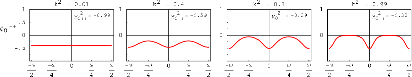
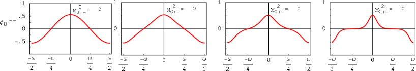
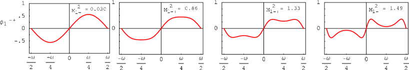
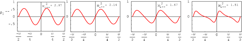
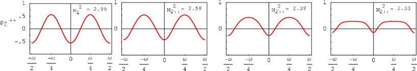
Figure 2: The normalized profiles of the first scalar modes for $k^{2}=0.01,\ 0.4,\ 0.8$ and $0.99$ (or $\omega=1.01\omega_{0},\ 1.34\omega_{0},\ 1.93\omega_{0}$ and $3.32\omega_{0}$, with $\omega_{0}=2\pi/m$). The mass eigenvalues are given in units of $m^{2}$. We have chosen $y_{0}=0$; for $y_{0}\neq 0$, $y$ one should be replaced by $y+y_{0}$.

It is worth emphasizing that the antisymmetry is also essential to develop a non-trivial vev: if symmetric solutions were allowed, then the constant vev would be chosen, as it is energetically more convenient.

3 Fermion Localization

A non-trivial vacuum of the scalar field will influence the phenomenology of all fields that couple to the scalar. Here we will consider the simplest scenario of the real scalar field coupled to fermions defined by the following Lagrangian density:

$${\cal L} = \bar{\psi}(x,y)\left[i\Gamma^{M}\partial_{M}-f\phi(x,y)-m_{0}\right]\psi(x,y)$$

$$+\frac{1}{2}\;\partial^{M}\phi(x,y)\;\partial_{M}\phi(x,y)-{\lambda\over 4}\left(|\phi|^{2}-{m^{2}\over\lambda}\right)^{2}\,,$$

with $\Gamma^{5}=i\gamma_{5}$. For simplicity, in the following discussion we will consider a massless 5D fermion, so that at the end we obtain chiral fermionic fields whose masses are generated exclusively through spontaneous symmetry breaking in the presence of Yukawa couplings. The absence of the mass term will be guaranteed by requiring the action to be symmetric under the following transformations:

$$\phi(x,y)\to-\phi(x,L/2-y)\;\;\;\;\;\;{\rm and}\;\;\;\;\;\;\psi(x,y)\to\gamma_{5}\psi(x,L/2-y)$$ (19)

We will adopt the following orbifold boundary conditions:

$$\psi(y)=\gamma_{5}\psi(-y)\;\;\;\;\;\;{\rm and}\;\;\;\;\;\;\psi(L/2+y)=\gamma_{5}\psi(L/2-y)\,,$$ (20)

so that right- and left-handed fermions are symmetric and antisymmetric with respect to $y=0$ and $y=L/2$ (which is identified with $y=-L/2$) . It is crucial to construct a chiral theory that disentangles left- and right-handed 4D fermions.

As we will see, once the field $\phi(x,y)$ acquires its non-trivial vev $\phi_{c}$ (see Eq. (7)), the mass spectrum of the KK modes of the fermion field is altered, from the “usual” tower of fermions with masses $m_{n}=2\pi n/L$. To find the spectrum and the eigenfunctions (KK modes) let us first decompose the field $\psi(x,y)$ in chiral components:

$$\psi = \psi_{\rm L}+\psi_{\rm R}$$ (21)

and let us now write the coupled Weyl equations of motion for these components:

$$i\partial/\ \psi_{\rm L}(x,y)-(\partial_{5}+f\phi_{c}(y))\psi_{\rm R}(x,y)=0$$ (22)

$$i\partial/\ \psi_{\rm R}(x,y)+(\partial_{5}-f\phi_{c}(y))\psi_{\rm L}(x,y)=0\,.$$ (23)

Now, we want to separate variables for each chiral field

$$\psi_{\rm L}(x,y) = \psi_{x}^{\rm L}(x)\ \psi^{\rm L}_{y}(y)$$ (24)

$$\psi_{\rm R}(x,y) = \psi_{x}^{\rm R}(x)\ \psi^{\rm R}_{y}(y)\,,$$ (25)

which gives

$$i\partial/\ \psi_{x}^{\rm L}-m_{n}\psi_{x}^{\rm R}=0, \ \ (\partial_{y}+f\phi_{c}(y))\psi^{\rm R}_{y}=m_{n}\psi^{\rm L}_{y}$$ (26)

$$i\partial/\ \psi_{x}^{\rm R}-m_{n}\psi_{x}^{\rm L}=0, \ \ (-\partial_{y}+f\phi_{c}(y))\psi^{\rm L}_{y}=m_{n}\psi^{\rm R}_{y}\,.$$ (27)

To obtain separate equations for the functions $\psi^{\rm L}_{y}$ and $\psi^{\rm R}_{y}$ we apply the operator $(-\partial_{5}+f\phi_{c})$ to the second equation in (26) and $(\partial_{5}+f\phi_{c})$ to the second one in (27), and get

$$\left[-\partial_{y}^{2}+\left(f\phi_{c}\right)^{2}\mp f\phi_{c}^{\prime}-m^{2}_{n}\right]\psi^{\rm R/L}_{y}=0$$

$${\rm or}\hskip 85.35826pt\$$

$$\left[-\partial_{y}^{2}+V_{\rm R/L}-m^{2}_{n}\right]\psi^{\rm R/L}_{y}=0$$ (28)

In general, since left- and right-handed profiles are solutions of different equations, we can expect different properties of $\psi^{\rm L}_{y}$ and $\psi_{y}^{\rm R}$, so that the theory is chiral, as we demanded. The “difference” between chiralities is controlled by the Yukawa coupling $f$ inside the potentials

$$V_{\rm R/L}\equiv\left(f\phi_{c}\right)^{2}\mp f\phi_{c}^{{}^{\prime}}=(\delta\ k)^{2}\ {\rm sn}^{2}\!\left(s,k^{2}\right)\mp(\delta\ k)\ {\rm cn}\!\left(s,k^{2}\right)\ {\rm dn}\!\left(s,k^{2}\right)\,.$$ (29)

Equations (28) have the form of the Hill’s equation, and it is known that if $P$ is the period of the equation, there will exist periodic solutions, of period $P$ or $2P$, and of defined even or odd parity. For each of these solutions there will be a specific eigenvalue $(m^{\rm R/L}_{n})^{2}$. In our case the required degeneracy of left- and right-handed modes will be guaranteed for all solutions of both equations. If the periodic background vev has some extra symmetry, it is possible to address this issue before actually solving Eqs. (28).

Let the background vev $\phi_{c}$ be periodic, of period $\omega$, i.e. $\ \phi_{c}(y+\omega)=\phi_{c}(y)$. Assume that this background vev also satisfies the relation

$$\phi_{c}(y+\omega/2)=-\phi_{c}(y)$$ (30)

If this is the case, we immediately see that

$$V_{\rm R}(y+\omega/2) = V_{\rm L}(y)\,.$$ (31)

This means that all periodic solutions of both equations will have exactly the same spectrum, the solutions being just shifted by $\omega/2$. Therefore it is sufficient to solve only one of the equations (R or L) and find the corresponding spectrum. The translational symmetry (31) will then immediately give the general solutions (with the same spectrum) to the other equation. With the general solutions of both equations, one can then impose the boundary conditions we have chosen for each chiral fermion, and get the final solutions for the fermion modes. It turns out that the solution of $\phi_{c}$ from Eq. (7) satisfies the relation (30). In Fig. 3 we plot the potentials $V_{\rm R}$ and $V_{\rm L}$ for selected values of $k^{2}$ (that determines the period $\omega$).

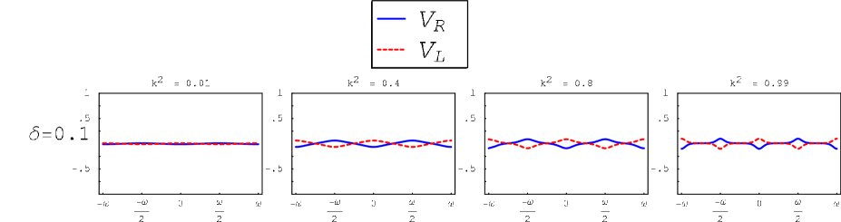
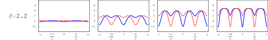
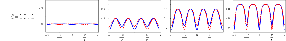
Figure 3: The profiles of the potentials $V_{\rm R}$ and $V_{\rm L}$ for $k^{2}=0.01,\ 0.4,\ 0.8$ and $0.99$ (or $\omega=1.01\omega_{0},\ 1.34\omega_{0},\ 1.93\omega_{0}$ and $3.32\omega_{0}$, with $\omega_{0}=2\pi/m$) and for $\delta=0.1,\ 1$ and $10$. We have chosen $y_{0}=0$; for $y_{0}\neq 0$, $y$ should be replaced by $y+y_{0}$. (Note the scale changes.)

We will now solve the R equation (and therefore get also the L solutions, thanks to the translational symmetry) and show the main results here. We will refer the reader to the Appendix for a more detailed derivation.

Using the background solution $\phi_{c}$ from Eq. (7) one can find that the unnormalized chiral zero mode consistent with the boundary condition (20) has quite a simple form:

$$\psi_{0}^{\rm R}(y)\propto\left[{\rm dn}\!\left({m\over\sqrt{k^{2}+1}}\ y,\ k^{2}\right)+k\ {\rm cn}\!\left({m\over\sqrt{k^{2}+1}}\ y,\ k^{2}\right)\right]^{\delta}\;\;{\rm and}\;\;\psi_{0}^{\rm L}(y)=0\,,$$ (32)

where $\delta=\sqrt{2f^{2}/\lambda}$. This solution is exact and we can see the behaviour of this chiral mode for different compactification scales (i.e. $k^{2}$) and for different values of $\delta$ in Fig. 4. The figure illustrates the relevance of the Yukawa coupling ($\propto\delta$) for the efficiency of the localization of the fermionic KK modes. It is also seen that it is easier for a given strength of the Yukawa coupling, to obtain the localization for the large extra dimension (and thus for large $k^{2}$).

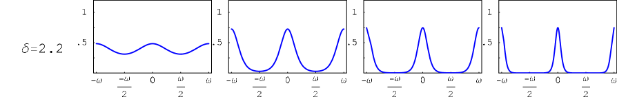
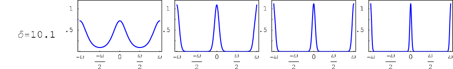
Figure 4: The profile of the normalized zero mode $\psi_{0}^{\rm R}$ for $k^{2}=0.01,\ 0.4,\ 0.8$ and $0.99$ (or $\omega=1.01\omega_{0},\ 1.34\omega_{0},\ 1.93\omega_{0}$ and $3.32\omega_{0}$, with $\omega_{0}=2\pi/m$) and with $\delta=0.1,\ 2.2$ and $10.1$. We have chosen $y_{0}=0$; for $y_{0}\neq 0$, $y$ should be replaced by $y+y_{0}$.

The rest of the modes cannot be written in such a compact form as the zero mode; however, it can be given in terms of convergent infinite trigonometric series. Their spectrum can be found by numerically solving a transcendental equation for each mass eigenvalue. Once the boundary conditions are imposed, we have

$$\psi_{2n}^{\rm R}(y) \propto \psi_{0}(y)\ \ CI^{2n}_{\omega}\!\!\left[\ {\rm am}\!\left({m\over 2}{(1+k)\over\sqrt{k^{2}+1}}\ y,\ {4k\over(1+k)^{2}}\right)\right]$$ (33)

$$\psi_{2n+1}^{\rm R}(y) \propto \psi_{0}(y)\ \ CI^{2n+1}_{2\omega}\!\!\left[\ {\rm am}\!\left({m\over 2}{(1+k)\over\sqrt{k^{2}+1}}\ y,\ {4k\over(1+k)^{2}}\right)\right]$$ (34)

$$\psi_{2n}^{\rm L}(y) \propto {\psi_{0}(y+\omega/2)}\ \ SI^{2n}_{\omega}\!\!\left[\ {\rm am}\!\left({m\over 2}{(1+k)\over\sqrt{k^{2}+1}}(y+\omega/2),\ {4k\over(1+k)^{2}}\right)\right]$$ (35)

$$\psi_{2n+1}^{\rm L}(y) \propto {\psi_{0}(y+\omega/2)}\ \ CI^{2n+1}_{2\omega}\!\!\left[\ {\rm am}\!\left({m\over 2}{(1+k)\over\sqrt{k^{2}+1}}(y+\omega/2),\ {4k\over(1+k)^{2}}\right)\right]\,,$$ (36)

where

$$\psi_{0}(y)=\left[{\rm dn}\!\left({m\over\sqrt{k^{2}+1}}\ y,\ k^{2}\right)+k\ {\rm cn}\!\left({m\over\sqrt{k^{2}+1}}\ y,\ k^{2}\right)\right]^{\delta}\$$ (37)

and $\omega={4\sqrt{1+k^{2}}\over m}K(k^{2})$ is the period of $\phi_{c}(y)$. Finally, ${\rm am}\!\left(x,m\right)$ is the Jacobian elliptic amplitude.

The series $CI^{2n}_{\pi}(t)$, $SI^{2n}_{\pi}(t)$ and $CI^{2n+1}_{2\pi}(t)$ are the periodic solutions (of period $\pi$ and $2\pi$ in the $t$ variable) of the generalized Ince equation [8] (it is a four-parameter, second-order differential equation, but in our case the parameter $d$ in [8] is zero, making the equation slightly simpler; see the Appendix for more details). The $C$ and $S$ indicate the parity of the series ($C$-even and $S$-odd). These generalized Ince solutions are given by:

$$CI^{2n}_{\pi}(t) = \sum^{\infty}_{r=0}A^{2n}_{2r}\cos{2rt}$$ (38)

$$SI^{2n}_{\pi}(t) = \sum^{\infty}_{r=1}B^{2n}_{2r}\sin{2rt}$$ (39)

$$CI^{2n+1}_{2\pi}(t) = \sum^{\infty}_{r=0}C^{2n+1}_{2r+1}\cos{(2r+1)t}\,,$$ (40)

where $n=1,2,3,\dots$. The coefficients $A^{2n}_{2r}$, $B^{2n}_{2r}$ and $C^{2n+1}_{2r+1}$ satisfy three-term recurrence relations, as given in the Appendix. It could be shown that $\psi_{2n}^{\rm R/L}(y)$ and $\psi_{2n+1}^{\rm R/L}(y)$ have periods $\omega$ and $2\omega$, respectively. We remind the reader that the scalar modes also had two periods, of $\omega/2$ and $\omega$, meaning that together, the wave functions of scalars and fermions have a total of three different periodicities.

As for the fermionic mass eigenvalues, there is a potential problem for the solutions of period $\omega$. The even right handed solutions ($CI^{2n}_{\omega}$), when shifted by $\omega/2$, give even solutions, and therefore cannot be the odd left-handed modes. To have the odd left-handed modes, we need to adopt the odd right-handed solutions ($SI^{2n}_{\omega}$) and shift them by $\omega/2$. But a priori these are two different solutions, and they are not necessarily degenerate, as they should since we are solving for the left and right chiral components of the same mode. However, it can be proved [8] that the two different solutions $CI^{2n}_{\omega}$ and $SI^{2n}_{\omega}$ of our particular generalized Ince equation have same eigenvalues (as needed) because the transcendental equations for $A^{2n}_{2r}$ and $B^{2n}_{2r}$, which set the eigenvalues, are the same (see the Appendix), even though the two solutions are different. Therefore the two chiral modes $\psi_{2n}^{\rm R}(y)$ and $\psi_{2n}^{\rm L}(y)$ will have the same mass eigenvalue.

In the case of the solutions of period $2\omega$, the degeneracy of the two chiral components is guaranteed since they are exactly the same solution, but shifted by $\omega/2$ (they have opposite parities because the period is $2\omega$, and therefore the parity changes when shifting them by $\omega/2$). A different transcendental equation for $C^{2n+1}_{2r+1}$ will set the masses of these $2\omega$ modes $\psi_{2n+1}^{\rm R/L}(y)$.

The complete spectrum can be very easily solved numerically, and Figs. 5, 6 and 7 show the spectrum of the first fermion modes as a function of $k$, and for three different values of $\delta$.

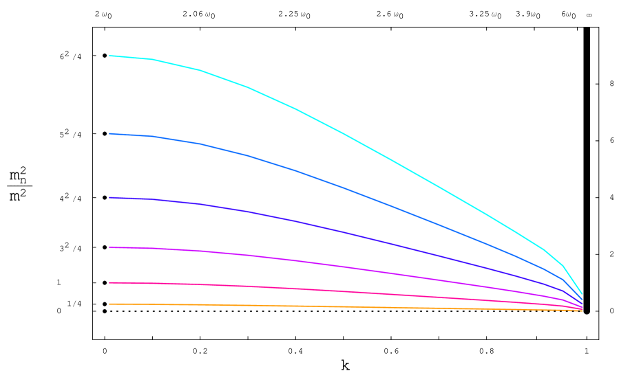
Figure 5: The mass variation of the first 7 modes with respect to the size of the extra dimension (i.e. the value of $k$). The spectrum goes from the discrete $n^{2}$ type spectrum at $k=0$ to the continuum spectrum for the case $k=1$, represented by the thick black vertical line. Here we have taken $\delta=0.1$

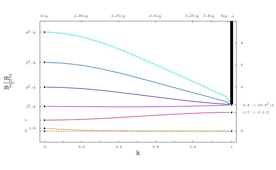
Figure 6: Same as the previous figure, but for $\delta=2.2$. Some discrete modes survive in the $k=1$ limit.

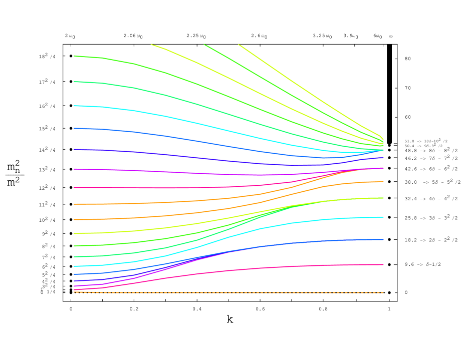
Figure 7: Same as the previous figure, but for the first 22 modes and with $\delta=10.1$. Some more discrete modes survive in the $k=1$ limit.

Before going further, it is instructive to consider the two limiting cases ($k\to 0$) and ($k\to 1$), which have known solutions and spectra. First let us define $s={m\over\sqrt{k^{2}+1}}\ y$, so that Eqs. (28) read

$$\left[-\frac{d^{2}}{ds^{2}}+(\delta\ k)^{2}\ {\rm sn}^{2}\!\left(s,k^{2}\right)\mp(\delta\ k)\ {\rm cn}\!\left(s,k^{2}\right)\ {\rm dn}\!\left(s,k^{2}\right)-(k^{2}+1){m^{2}_{n}\over m^{2}}\right]\psi^{\rm R/L}_{s}=0\,,$$ (41)

where ${\rm cn}(s,k^{2})$ and ${\rm dn}(s,k^{2})$ are the Jacobi elliptic cosine-amplitude and delta-amplitude respectively.

1. Keeping only the leading terms in the limit $k\to 0$, the equation simplifies to

   $$\left(\frac{d^{2}}{ds^{2}}+{m^{2}_{n}\over m^{2}}\right)\psi^{\rm R/L}_{s}=0\,,$$ (42)

   with $s=my$. In this limit we obtain the following solutions (consistent with the boundary conditions (20)) for the fermionic KK modes:

   $$\psi_{n}^{\rm R}(y)\propto\cos\left(n\;{\pi\over\omega_{0}}y\right)\;\;\;\;\;\;{\rm and}\;\;\;\;\;\;\psi_{n}^{\rm L}(y)\propto\sin\left(n\;{\pi\over\omega_{0}}y\right)\,,$$ (43)

   with $\omega_{0}=2\pi/m$ . Note that, in the limit $k\to 0$, the Schrödinger-like equation is not a periodic equation, and we therefore have to fix the period by hand; here we have assumed that the size of the extra dimension is $2\omega_{0}$, as this matches the general solution of the general equation (28). The spectrum we expect is therefore $m_{n}^{2}=n^{2}\;{m^{2}\over 4\ }$ for $n=0,1,2,\dots$, and Figs. 5, 6 and 7 show how our solutions do approach these limiting values. Note that in this case, even though the theory is chiral, there is no localization of fermions observed.

2. When ($k\to 1$) (which means $\omega\to\infty$), we have $\ {\rm sn}^{2}(s,k^{2})\to\tanh^{2}{s}\$ and $\ {\rm cn}(s,k^{2})\ {\rm dn}(s,k^{2})\to{\rm sech}^{2}(x)$.

   With this limiting behaviour, Eqs. (41) become

   $$\left(-\frac{d^{2}}{ds^{2}}+\delta^{2}\tanh^{2}{s}\mp\delta\ {\rm sech}^{2}{s}\ -2{m^{2}_{n}\over m^{2}}\right)\psi^{\rm R/L}_{s} = 0\,,$$ (44)

   for $s=m/\sqrt{2}\ y$. This is the limit discussed so far in the literature, see [2] and [3]. Since the $y$-direction is no longer compact, we obtain in this case both the discrete and the continuum spectrum of eigenvalues. This could be observed in Figs. 5, 6 and 7 where the thick vertical line represents the continuum spectrum while the discrete eigenvalues are showed as separated “energy” levels.

   Using SUSY quantum mechanics methods, it was shown in [2] that when the eigenvalue $m_{n}$ is such that $m_{n}^{2}<\delta^{2}$ (in those authors notation $M^{2}<w^{2}$) the first $n_{B}$ fermion modes (with $0\leq n_{B}<\delta$) are bound states with a very simple discrete spectrum given by $m^{2}_{n}=(n_{B}\ \delta-n_{B}^{2}/2)$. When $m_{n}^{2}>\delta^{2}$ the spectrum becomes a continuum of states. Again, Figs. 5, 6 and 7 show how this limiting behaviour is recovered by our solutions.

The early attempts to pass from the case ($k=1$) (infinite extra dimension) to the compact case ($k<1$) seem to have missed half the available spectrum of fermionic modes. The reason for this is as follows. If in a compact dimension with a periodic background vev of period $\omega$, we force the size of the extra dimension to be also $\omega$, all the fermionic states of period $2\omega$ will be automatically dismissed by the $\omega$ periodicity condition. This imposition now seems rather arbitrary and awkward, since it does not come from any symmetry, but is, as we now know, extremely constraining. Of course, the size of the compact space must be a multiple of the background period $\omega$, and because $2\omega$ is the minimum period that contains all the possible KK modes of all matter fields, it seems natural for $2\omega$ to be the size of the extra dimension. Close to the limit ($k\to 1$), we can see how some of the ($k=1$) “fat-brane” modes split into period $\omega$ and period $2\omega$ modes. The structure follows a curious pattern:

• The zero-mode $\psi_{0}$ (of period $\omega$) and the first-level-mode $\psi_{1}$ (of period $2\omega$) become degenerate (and massless) in the ($k\to 1$) limit. This means that when $k$ is close to 1, but still smaller than 1, we do have a chiral zero mode in the spectrum, but also an extremely light first-level massive fermion (as seen in Fig. 8, when $k^{2}=0.99$ (or $\omega=3.32\omega_{0}$), we have $m_{1}^{2}\sim 10^{-49}m^{2}$). This feature seems to be also very advantageous for model building (e.g. explaining mass hierarchies or modeling the neutrino sector).

• The next fermion level, $\psi_{2}$, of period $\omega$ (for $\delta>1$ and values of $k$ still close to 1), comes as a single state, with mass squared $\sim(\delta-1/2)m^{2}$.

• If ($\delta>2$), there is at least another limiting discrete bound state. We see that, in this case, three fermion modes, $\psi_{3}$, $\psi_{4}$ and $\psi_{5}$, get close together and become nearly degenerate, when $k$ is close to 1, the mass splitting between them being extremely small compared to the gap between them and the previous mode $\psi_{2}$. This feature again seems quite interesting.

• The next level, if $\delta$ is big enough, comes alone, and the next three together. This pattern repeats itself until the levels reach the continuum limit of the ($k=1$) case. Then all the modes become roughly evenly separated, and for the higher modes we recover the typical tower of masses following the $n^{2}\over 4$ structure.

Figures 8, 9, 10 and 11 show the first modes $\psi_{1}^{\rm L/R}$, $\psi_{2}^{\rm L/R}$, $\psi_{3}^{\rm L/R}$ and $\psi_{4}^{\rm L/R}$ and their mass, for different values of $\delta$ and different compactification scales.

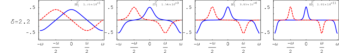
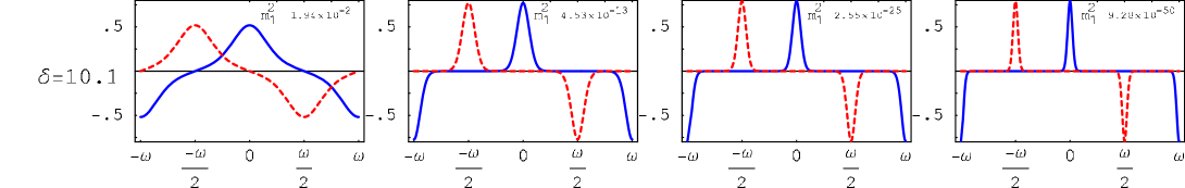
Figure 8: The profile of the normalized mode $\psi^{\rm R/L}_{1}$, of period $2\omega$, for $k^{2}=0.01,\ 0.4,\ 0.8$ and $0.99$ (or $\omega=1.01\omega_{0},\ 1.34\omega_{0},\ 1.93\omega_{0}$ and $3.32\omega_{0}$, with $\omega_{0}=2\pi/m$) and with $\delta=0.1,\ 2.2$ and $10.1$. The mass eigenvalues are given in units of $m^{2}$.

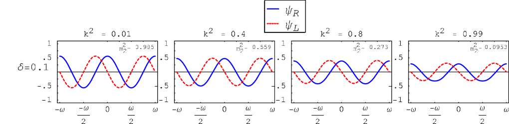
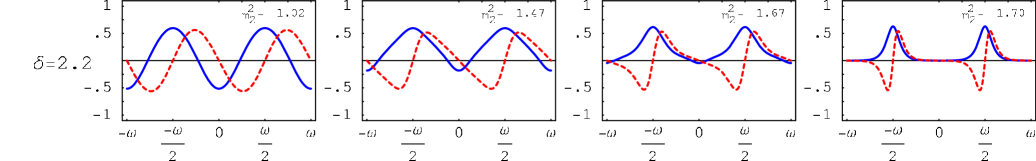
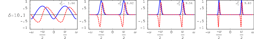
Figure 9: The profile of the normalized mode $\psi^{\rm R/L}_{2}$, of period $\omega$, for $k^{2}=0.01,\ 0.4,\ 0.8$ and $0.99$ (or $\omega=1.01\omega_{0},\ 1.34\omega_{0},\ 1.93\omega_{0}$ and $3.32\omega_{0}$, with $\omega_{0}=2\pi/m$) and with $\delta=0.1,\ 2.2$ and $10.1$. The mass eigenvalues are given in units of $m^{2}$.

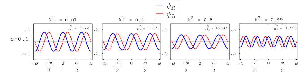
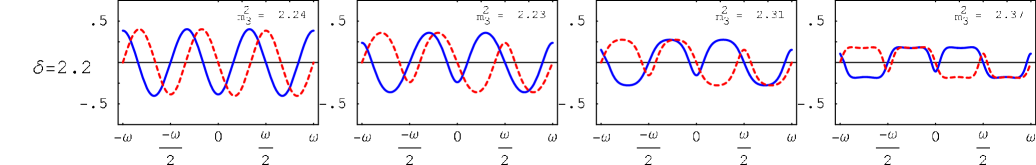
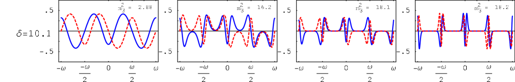
Figure 10: The profile of the normalized mode $\psi^{\rm R/L}_{3}$, of period $2\omega$, for $k^{2}=0.01,\ 0.4,\ 0.8$ and $0.99$ (or $\omega=1.01\omega_{0},\ 1.34\omega_{0},\ 1.93\omega_{0}$ and $3.32\omega_{0}$, with $\omega_{0}=2\pi/m$) and with $\delta=0.1,\ 2.2$ and $10.1$. The mass eigenvalues are given in units of $m^{2}$.

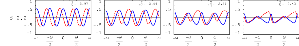
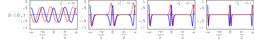
Figure 11: The profile of the normalized mode $\psi^{\rm R/L}_{4}$, of period $\omega$, for $k^{2}=0.01,\ 0.4,\ 0.8$ and $0.99$ (or $\omega=1.01\omega_{0},\ 1.34\omega_{0},\ 1.93\omega_{0}$ and $3.32\omega_{0}$, with $\omega_{0}=2\pi/m$) and with $\delta=0.1,\ 2.2$ and $10.1$. The mass eigenvalues are given in units of $m^{2}$.

4 Conclusions

We have discussed the low-energy consequences of a non-trivial real scalar-field background in the context of one compact extra dimension. The periodic background that appears within (1+4)-dimensional $\phi^{4}$ theory was found, this solution being the analogue of the kink–antikink approximate solution discussed so far in the literature. We have determined analytically the excitations above the background and their spectrum. It was found that, in the presence of the non-trivial solution, there exists a minimal size of the extra dimension that is determined by the mass parameter of the scalar potential: $L_{0}=2\omega_{0}=4\pi/m$. We have shown that imposing orbifold antisymmetry boundary conditions allows the elimination of a negative mass squared Kaluza–Klein ground-state mode that otherwise would cause an instability of the system. The localization of fermionic modes in the presence of the non-trivial background was discussed in detail. A simple and exact solution for the zero-mode fermionic states was found and the solution for non-zero modes in terms of trigonometric series was constructed. The fermionic mass spectrum turned out to be very interesting, with possible phenomenological consequences for constructing a realistic theory based on a non-trivial background solution. Limiting cases of small harmonic oscillations and very large extra dimensions (the case considered in the literature so far) were discussed and used as a test of the general solutions for the fermionic Kaluza–Klein modes found in this work. We have shown that the natural size of the extra dimension is twice as large as the period of the scalar background solution.

ACKNOWLEDGEMENTS

B.G. thanks Mikhail Shaposhnikov for an useful discussion on the periodic kink-like solutions. The authors thank John Gunion for his contribution at the early stages of this work. B.G. is supported in part by the State Committee for Scientific Research under grant 5 P03B 121 20 (Poland). M.T. is supported by the Davis Institute for High Energy Physics. This work was also supported by a joint Warsaw–Davis collaboration grant from the National Science Foundation and the Polish Academy of Science.

Appendix

We are interested in finding all the periodic solutions of the equation:

$$\left[-\partial_{y}^{2}+\left(f\phi_{c}\right)^{2}-f\phi_{c}^{\prime}-m^{2}_{n}\right]\psi^{\rm R}_{y}=0\,.$$ (A-1)

With these solutions, we can immediately get solutions to

$$\left[-\partial_{y}^{2}+\left(f\phi_{c}\right)^{2}+f\phi_{c}^{\prime}-m^{2}_{n}\right]\psi^{\rm L}_{y}=0\,,$$ (A-2)

as explained in the text, by simply doing a space translation of $\omega/2$.

It will prove useful to perform the redefinition

$$\psi_{y}^{\rm R}(y)=v_{y}^{\rm R}(y)\exp\left\{-f\int^{y}_{y_{0}}d{\tilde{y}}\ \phi_{c}(\tilde{y})\right\}\,.$$ (A-3)

We then have an equation for $v_{y}^{\rm R}(y)$:

$$-{d^{2}\over dy^{2}}v_{y}^{\rm R}+2f\phi_{c}{d\over dy}v_{y}^{\rm R}-m^{2}_{n}v_{y}^{\rm R}=0\,.$$ (A-4)

We see that it is easy to solve either Eq. (A-4) or Eq. (26) for the zero-mode fermion ($m_{n}=0$). The chosen boundary conditions (20) imply that the solution reads:

$$\psi_{0}^{\rm R}(y)\propto\exp\left\{-f\int_{y_{0}}^{y}d{\tilde{y}}\ \phi_{c}(\tilde{y})\right\}\;\;\;\;\;\;{\rm and}\;\;\;\;\;\;\;\;\;\;\;\;\psi_{0}^{\rm L}(y)=0\,.$$ (A-5)

Now, using the background solution $\phi_{c}$ from Eq. (7) we get the unnormalized chiral mode

$$\psi_{0}^{\rm R}(y)\propto\left[{\rm dn}\!\left({m(y-y_{0})\over\sqrt{k^{2}+1}},k^{2}\right)+k\ {\rm cn}\!\left({m(y-y_{0})\over\sqrt{k^{2}+1}},k^{2}\right)\right]^{\delta}\;\;{\rm and}\;\;\psi_{0}^{\rm L}(y)=0\,,$$ (A-6)

where $\delta=\sqrt{2f^{2}/\lambda}$. This solution is exact.

If we now insert the periodic background solution $\phi_{c}$ in Eq. (A-4) we get the Picard elliptic equation [8] for the function $v_{y}^{\rm R}$:

$$-{d^{2}\over dy^{2}}v_{y}^{\rm R}+2\delta m\sqrt{k^{2}\over k^{2}+1}\ {\rm sn}\left({m(y-y_{0})\over\sqrt{k^{2}+1}},\ k^{2}\right){d\over dy}v_{y}^{\rm R}-m^{2}_{n}v_{y}^{\rm R}=0$$ (A-7)

Before going any further, we now need to use the known transformation formula for the elliptic sine function:

$${\rm sn}\left((1+\sqrt{1-\tilde{k}^{2}})\ u,\ \left[{1-\sqrt{1-\tilde{k}^{2}}\over 1+\sqrt{1-\tilde{k}^{2}}}\right]^{2}\right)=(1+\sqrt{1-\tilde{k}^{2}})\ {{\rm sn}\left(u,\tilde{k}^{2}\right)\ {\rm cn}\left(u,\tilde{k}^{2}\right)\over{\rm dn}\left(u,\tilde{k}^{2}\right)}$$ (A-8)

With this at hand we now redefine $u={m\over 2}{(1+k)\over\sqrt{k^{2}+1}}(y-y_{0})$ and we obtain:

$$-{d^{2}\over du^{2}}v_{u}^{\rm R}+2\delta\ \tilde{k}^{2}{{\rm sn}\left(u,\tilde{k}^{2}\right){\rm cn}\left(u,\tilde{k}^{2}\right)\over{\rm dn}\left(u,\tilde{k}^{2}\right)}{d\over du}v_{u}^{\rm R}-\beta_{n}v_{u}^{\rm R}=0$$ (A-9)

where $\tilde{k}^{2}={4k\over(1+k)^{2}}$ and $\beta_{n}=4{(k^{2}+1)\over(k+1)^{2}}{m_{n}^{2}\over m^{2}}$.

Now this can finally be brought to a simplified form of the generalized Ince equation[8] by a new change of variables, $\ \sin{t}={\rm sn}\left(u,\tilde{k}^{2}\right)$:

$$-(1-\tilde{k}^{2}\sin^{2}{t}){d^{2}\over dt^{2}}v_{t}^{\rm R}+(1+2\delta)\ \tilde{k}^{2}\sin{t}\cos{t}\ {d\over dt}v_{t}^{\rm R}-\beta_{n}v_{t}^{\rm R} = 0\,.$$ (A-10)

Written in its canonical form we have

$$(1+a\cos{2t}){d^{2}\over dt^{2}}v_{t}^{\rm R}+b\sin{2t}{d\over dt}v_{t}^{\rm R}-\lambda_{n}v_{t}^{\rm R} = 0\,,$$ (A-11)

where $\ a={\tilde{k}^{2}\over 2-\tilde{k}^{2}}={2k\over k^{2}+1}\ ,\ b=-(1+2\delta){2k\over k^{2}+1}\$ and $\lambda_{n}={(k+1)^{2}\over k^{2}+1}\beta_{n}=4{m_{n}^{2}\over m^{2}}$.

We will now recall some known results related to the special case of the generalized Ince equation from [8]. It is known that, for any real values of $a$ (satisfying $|a|<1$) and $b$, there exist infinitely many values of the parameter $\lambda_{n}$ such that Eq. (A-11) has an even or odd periodic solution, of period $\pi$ or $2\pi$. We will denote them as $\lambda^{\pi}_{2n}$, $\lambda^{2\pi}_{2n+1}$ and $\lambda^{2\pi}_{2n+2}$, where $n=0,1,2,3...$ In our case, for each of the $\lambda_{2n}^{\pi}$, there must be two linearly independent such solutions (except for the ground state $n=0$, which allows only one periodic solution). If and only if the parameter $\delta$ is an integer, there will be also two linearly independent periodic solutions of period $2\pi$, and then $\lambda^{2\pi}_{2n+1}=\lambda^{2\pi}_{2n+2}$. When $\delta$ is not an integer, then one of the two linearly independent solutions will be periodic, of period $2\pi$, but the other one will not be periodic. The $\lambda_{n}$’s satisfy the inequalities:

$$\lambda^{\pi}_{0}<\lambda^{2\pi}_{1}\leq\lambda^{2\pi}_{2}<\lambda^{\pi}_{2}<\lambda^{2\pi}_{3}\leq\lambda^{2\pi}_{4}<\lambda^{\pi}_{4}<\cdots\,,$$ (A-12)

where the equalities hold whenever $\delta$ is integer. In our specific case we have $\lambda^{\pi}_{0}=m_{0}=0$.

Since the solutions to Eq. (A-11) are even or odd and of period $\pi$ or $2\pi$, the solutions can be given with trigonometric series:

$$CI^{2n}_{\pi}(t)=\sum^{\infty}_{r=0}A^{2n}_{2r}\cos{2rt}\hskip 42.67912pt \ SI_{\pi}^{2n}(t)=\sum^{\infty}_{r=1}B^{2n}_{2r}\sin{2rt}$$ (A-13)

$$CI^{2n+1}_{2\pi}(t)=\sum^{\infty}_{r=0}C^{2n+1}_{2r+1}\cos{(2r+1)t} SI^{2n+2}_{2\pi}(t)=\sum^{\infty}_{r=0}D^{2n+2}_{2r+1}\sin{(2r+1)t}\ \ \ \$$ (A-14)

where $n=0,1,2,3,\dots$ The $CI$’s are even while the $SI$’s are odd functions of $t$. The periods are as follows: $\pi$ for $CI^{2n}_{\pi}$, $SI^{2n}_{\pi}$ and $2\pi$ for $CI^{2n+1}_{2\pi}$, $SI^{2n+2}_{2\pi}$ (they correspond to the periods $\omega$ and $2\omega$, respectively, in terms of the variable $y$). Now, we define

$$Q(r) = 2ar^{2}-br\ =\ {4k\over k^{2}+1}\ r\ \left(r+\delta+1/2\right)$$ (A-15)

$$Q^{*}(r) = 2Q(r-1/2)=\ {4k\over k^{2}+1}\ (2r-1)\ (r+\delta)\,.$$ (A-16)

The parameters $A^{2n}_{2r}$, $B^{2n}_{2r}$, $C^{2n+1}_{2r+1}$ and $D^{2n+2}_{2r+1}$ satisfy the following three term recurrence relations [8]:

$$-\lambda^{\pi}_{2n}A_{0}+Q(-1)A_{2} = 0$$ (A-17)

$$Q(r-1)A_{2r-2}+\left(4r^{2}-\lambda^{\pi}_{2n}\right)A_{2r}+Q(-r-1)A_{2r+2} = 0\hskip 85.35826pt$$ (A-18)

$$r=1,2,3,...$$

$$\left(4-\lambda^{\pi}_{2n}\right)B_{2}+Q(-2)B_{4} = 0$$ (A-19)

$$Q(r-1)B_{2r-2}+\left(4r^{2}-\lambda^{\pi}_{2n}\right)B_{2r}+Q(-r-1)B_{2r+2} = 0\hskip 85.35826pt$$ (A-20)

$$r=2,3,...$$

$$\left[Q^{*}(0)-2(\lambda^{2\pi}_{2n+1}-1)\right]C_{1}+Q^{*}(-1)C_{3} = 0$$ (A-21)

$$Q^{*}(r)C_{2r-1}+2\left[(2r+1)^{2}-\lambda^{2\pi}_{2n+1}\right]C_{2r+1}+Q^{*}(-r-1)C_{2r+3} = 0\hskip 85.35826pt$$ (A-22)

$$r=1,2,3,...$$

$$\left[-Q^{*}(0)-2(\lambda^{2\pi}_{2n+2}-1)\right]D_{1}+Q^{*}(-1)D_{3} = 0$$ (A-23)

$$Q^{*}(r)D_{2r-1}+2\left[(2r+1)^{2}-\lambda^{2\pi}_{2n+2}\right]D_{2r+1}+Q^{*}(-r-1)D_{2r+3} = 0\hskip 85.35826pt$$ (A-24)

$$r=1,2,3,...$$

The condition that the series (A-13) and (A-14) converge will set the characteristic values of $\lambda^{\pi/2\pi}_{i}$. These characteristic equations can be written in terms of infinite determinants [15] or, as we will do, as infinite continued fractions [13].

We need to remember that we are solving the equation for the right-hand fermion modes $\psi_{\rm R}^{n}$. The boundary conditions impose that these are even functions of $y$. So, we might be inclined to immediately disregard the solutions $SI_{\pi}^{2n}$ and $SI^{2n+2}_{2\pi}$. However, it turns out that they are needed to obtain the left-hand modes $\psi_{\rm L}^{n}$, which are odd functions of $y$. We do this by translating the general solutions of Eq. A-1, by $\omega/2$.

If we perform the translation of the period $\omega$ even solution of (A-1), constructed with $CI^{2n}_{\pi}$, we do get an even solution of (A-2). But we want $\psi_{\rm L}$ to be odd, and that solution is thus not good. What is needed is to compute the period $\omega$ odd solution of (A-1), constructed with $SI_{\pi}^{2n}$. The translated function will now be odd. As we said earlier, even and odd solutions of period $\pi$ (period $\omega$ in $y$ coordinate) of Eq. (A-1) are guaranteed to exist for the same specific eigenvalues.

The story is different for the period $2\omega$ solutions. Now the translation of the period $2\omega$ even solution of (A-1) constructed with $CI^{2n+1}_{2\pi}$ will give an odd solution of (A-2), which is exactly the solution for $\psi_{\rm L}$ that we need. Therefore the odd series $SI^{2n+1}_{2\pi}$ with coefficients $D_{2r+1}^{2n+2}$ will not be needed, since they correspond to odd solutions of (A-1) and to even solutions of (A-2), precisely the opposite parities needed.

Summarizing, the final solutions of (A-1) and (A-2) are as follows:

$$\psi_{2n}^{\rm R}(y) \propto\ \psi_{0}(y)\ \ CI^{2n}_{\omega}\!\!\left[\ {\rm am}\!\left({m\over 2}{(1+k)\over\sqrt{k^{2}+1}}\ y,\ {4k\over(1+k)^{2}}\right)\right]$$ (A-25)

$$\psi_{2n+1}^{\rm R}(y) \propto\ \psi_{0}(y)\ \ CI^{2n+1}_{2\omega}\!\!\left[\ {\rm am}\!\left({m\over 2}{(1+k)\over\sqrt{k^{2}+1}}\ y,\ {4k\over(1+k)^{2}}\right)\right]$$ (A-26)

$$\psi_{2n}^{\rm L}(y) \propto\ {\psi_{0}(y+\omega/2)}\ \ SI^{2n}_{\omega}\!\!\left[\ {\rm am}\!\left({m\over 2}{(1+k)\over\sqrt{k^{2}+1}}(y+\omega/2),\ {4k\over(1+k)^{2}}\right)\right]$$ (A-27)

$$\psi_{2n+1}^{\rm L}(y) \propto\ {\psi_{0}(y+\omega/2)}\ \ CI^{2n+1}_{2\omega}\!\!\left[\ {\rm am}\!\left({m\over 2}{(1+k)\over\sqrt{k^{2}+1}}(y+\omega/2),\ {4k\over(1+k)^{2}}\right)\right]\ \ \ \ \ \$$ (A-28)

where

$$\psi_{0}(y)=\left[{\rm dn}\!\left({m\over\sqrt{k^{2}+1}}\ y,\ k^{2}\right)+k\ {\rm cn}\!\left({m\over\sqrt{k^{2}+1}}\ y,\ k^{2}\right)\right]^{\delta}\$$ (A-29)

and $\omega={4\sqrt{1+k^{2}}\over m}K(k^{2})$ is the period of $\phi_{c}(y)$. Finally, ${\rm am}\!\left(x,m\right)$ is the Jacobian elliptic amplitude.

In order to find specific values of the eigenvalues such that these periodic solutions exist, we will only need two transcendental equations (infinite continued fractions equations) to find the values $\lambda^{\pi}_{2n}$ and $\lambda^{2\pi}_{2n+1}$. To simplify our notation, we will introduce the continued fraction notation:

$${a\over b+{c\over d+{e\over f+\cdots}}}={a\over b+}\ {c\over d+}\ {e\over f+}\cdots$$ (A-30)

Using the recurrence relations (A-20) and (A-22) (see §3.6 in [13] for the procedure) we find the two transcendental equations that fix all the values of $\lambda^{\pi}_{2n}$ and $\lambda^{2\pi}_{2n+1}$:

$${4-\lambda_{2n}^{\pi}}={Q(-2)Q(1)\over 16-\lambda_{2n}^{\pi}-}\ {Q(-3)Q(2)\over 36-\lambda_{2n}^{\pi}-}\ {Q(-4)Q(3)\over 64-\lambda_{2n}^{\pi}-}\ \cdots\ {Q(-N)Q(N-1)\over 4N^{2}-\lambda_{2n}^{\pi}-}\cdots$$ (A-31)

$$Q^{*}(0)+2-2\lambda^{2\pi}_{2n+1}={Q^{*}(-1)Q^{*}(1)\over 9-\lambda^{2\pi}_{2n+1}-}\ {Q^{*}(-2)Q^{*}(2)\over 25-\lambda^{2\pi}_{2n+1}-}\ \cdots\ {Q^{*}(-N)Q^{*}(N)\over(2N+1)^{2}-\lambda_{2n+1}^{2\pi}-}\cdots$$ (A-32)

These can easily be solved numerically.

References

- [1] V. A. Rubakov and M. E. Shaposhnikov, Phys. Lett. B 125, 136 (1983).
- [2] H. Georgi, A. K. Grant and G. Hailu, Phys. Rev. D 63, 064027 (2001) [arXiv:hep-ph/0007350].
- [3] P. Q. Hung and N. K. Tran, arXiv:hep-ph/0309115.
- [4] D. E. Kaplan and T. M. Tait, JHEP 0111, 051 (2001) [arXiv:hep-ph/0110126].
- [5] N. Arkani-Hamed and M. Schmaltz, Phys. Rev. D 61, 033005 (2000) [arXiv:hep-ph/9903417].
- [6] M. B. Voloshin, Yad. Fiz. 21, 1331 (1975), G. R. Dvali and M. A. Shifman, Phys. Lett. B 396, 64 (1997) [Erratum-ibid. B 407, 452 (1997)] [arXiv:hep-th/9612128].
- [7] R. Jackiw and C. Rebbi, Phys. Rev. Lett. 36, 1116 (1976).
- [8] W. Magnus and S. Winkler, Hill’s equation (Interscience Publishers, New York, 1966).
- [9] B. J. Harrington, Phys. Rev. D 18, 2982 (1978).
- [10] J. L. Richard and A. Rouet, Nucl. Phys. B 183, 251 (1981).
- [11] J.A. Espichan Carrillo, A. Maia, Jr. and V.M. Mostepanenko, Int. J. Mod. Phys. A 15, 2645 (2000) [arXiv:hep-th/9905151].
- [12] A. Erdélyi et al., Higher transcendental functions (McGraw-Hill Book Company, Inc., New York, 1953), vol. 1.
- [13] F. M. Arscott, Periodic differential equations (MacMillan Company, New York, 1964).
- [14] S. Coleman, Aspects of symmetry (Cambridge University Press, 1985).
- [15] Z. X. Wang and D. R. Guo, Special functions (World Scientific Publishing Co., Singapore, 1989).