Charm production in diffractive deep inelastic scattering

Abstract

The diffractive open charm production is computed in perturbative QCD formalism and in the Regge approach. The results are compared with recent data on charm diffractive structure function measured at DESY-HERA. Our results demonstrate that this observable can be useful to discriminate the QCD dynamics.

1 Introduction

The study of electroproduction at small $x$ has lead to the improvement of our understanding of QCD dynamics at the interface of perturbative and nonperturbative physics. In particular, the discovery of diffractive events in this process at HERA has triggered a large amount of experimental and theoretical work and greatly increased our knowledge of the physics of diffraction (For recent reviews see Refs. [1, 2, 3]). Diffractive processes in deep-inelastic scattering (DIS) are of particular interest, because the hard photon in the initial state gives rise to the hope that, at least in part, the scattering amplitude can be calculated in pQCD. Moreover, DIS exhibits the nice feature of having a colorless particle, the virtual photon, in the initial state. The main theoretical interest in diffraction is centered around the interplay between the soft and hard physics. Hard physics is associated with the well established parton picture and perturbative QCD, and is applicable to processes for which a large scale is present. Soft dynamics on the other hand, linked for example with the total cross section of hadron scattering, is described by nonperturbative aspects of QCD. The ability to separate clearly the regimes dominated by soft and hard processes is essential in exploring QCD at both quantitative and qualitative level.

Recently, we have proposed the analyzes of the slope of diffractive structure function as a potential observable to disentangle the leading dynamics at $ep$ diffractive processes [4, 5]. The predictions for the behavior of this quantity are strongly dependent of the QCD dynamics dominant in the kinematical region (For a recent discussion see Ref. [6]). Similarly, the study of the diffractive final state can lead to further progress in the direction of obtaining a coherent picture of the diffraction. In particular, charm production looks promising in this respect, as predictions for this process widely differ among several models [7, 8, 9, 10, 11]. Recently, the ZEUS collaboration has presented its results for the measurement of the open-charm contribution to the diffractive proton structure function [12]. Consequently, a more detailed analyzes of the models and a comparison between their predictions and the experimental data is on time. Here the diffractive open charm production is computed in perturbative QCD formalism and in the Regge approach. As these models are based on very distinct assumptions, it allows shed light into the leading dynamics at $ep$ diffractive processes.

This paper is organized as follows. In the next section, we summarize the main formulas for computation of the open charm diffractive structure function. One presents it in the transverse momentum representation in the perturbative QCD approach. Moreover, the diffractive production of open charm is calculated in a Regge inspired approach, where charm is produced by boson gluon fusion and which directly depends on the gluon distribution of the Pomeron. In the last section, we compare both approaches with current experimental measurements from DESY-HERA collider and present our discussions and conclusion.

2 Diffractive production of open charm in deep inelastic scattering

Before introducing the main expressions needed to our calculation, let’s introduce the kinematical definitions in diffractive DIS (DDIS) $\gamma^{*}\,(q)+p\,(P)\rightarrow X\,(M_{X})\,p\,(P^{\prime})$ with $X$ being the diffractive final state. The kinematics is defined as follows,

$$x=\frac{-q^{2}}{2P.q}\,,\hskip 19.91684ptx_{{IP}}=\frac{q.(P-P^{\prime})}{q.P}\,,\hskip 19.91684pt\beta=\frac{-q^{2}}{2q.(P-P^{\prime})}\approx\frac{Q^{2}}{Q^{2}+M_{X}^{2}}\,,$$ (1)

where $q$, $P$ and $P^{\prime}$ are the four-momenta of the virtual boson, the incident proton and the remnant colorless final state, respectively. The invariant mass of the diffractive final state is labeled $M_{X}$. The variable $x$ is the momentum fraction of the proton carried by the partons (quarks or gluons), the Bjorken variable, and by definition $x=\beta\,x_{{IP}}$. As usual, $Q^{2}=-q^{2}$ is the photon virtuality.

At high energies, $x_{{IP}}$ may be interpreted as the fraction of the proton four-momentum carried by the diffractive exchange, the colorless Pomeron. The $\beta$ variable is the fraction of the four-momentum of the diffractive exchange carried by the parton interacting with the virtual boson. The diffractive structure function is defined in analogy with the decomposition of the unpolarized total $ep$ cross section as,

$$\frac{d^{3}\sigma_{ep\rightarrow epX}}{dx_{{IP}}\,d\beta\,dQ^{2}}=\frac{4\pi\alpha^{2}}{xQ^{4}}\left\{1-y+\frac{y^{2}}{2}\right\}F_{2}^{D(3)}(x_{{IP}},\beta,Q^{2})\,.$$ (2)

Since the first observation of diffractive DIS at HERA, several attempts have been made to compare the data with the Regge and QCD-based models [14, 15, 16] (See also [17, 18, 19]). In general, these models provide a reasonable description of the present data on the diffractive structure function $F_{2}^{D(3)}$, although based on quite distinct frameworks. Furthermore, the QCD factorization theorem has been proven to be valid for $F_{2}^{D(3)}$ [20], with the immediate consequence that the DGLAP evolution equations [21] should describe the scaling violations observed in this observable. However, there are no constraints on the gluon momentum distribution since the momentum sum rule does not formally apply.

Here, we study in detail the predictions for the charm component of the diffractive structure function, $F_{2}^{D(3)\,\mathrm{charm}}$, which is directly sensitive to the gluonic content of the pomeron, considering two distinct approaches: i) a Regge inspired model [13, 14], where the diffractive production is dominated by a nonperturbative Pomeron, and the diffractive structure function is obtained using the Ingelman-Schlein ansatz [22]. ii) a pQCD approach [15, 16] where the diffractive process is modeled as the scattering of the photon Fock states with the proton through a gluon ladder exchange (in the proton rest frame). Below we present a brief review of the main assumptions of these models.

In the perturbative QCD framework, there are successful analysis describing the diffractive structure function [15, 16]. The underlying physical picture is that, in the proton rest frame, diffractive DIS is described by the interaction of the photon Fock states ($q\bar{q}$ and $q\bar{q}g$ configurations) with the proton through a Pomeron exchange, modeled as a two hard gluon exchange. The corresponding structure function contains the contribution of $q\bar{q}$ production to both the longitudinal and the transverse polarization of the incoming photon and of the production of $q\bar{q}g$ final states from transverse photons. The basic elements of this approach are the photon light-cone wave function and the nonintegrated gluon distribution (or dipole cross section in the dipole formalism). For elementary quark-antiquark final state, the wave functions depend on the helicities of the photon and of the (anti)quark. For the $q\bar{q}g$ system one considers a gluon dipole, where the pair forms an effective gluon state associated in color to the emitted gluon and only the transverse photon polarization is important. The interaction with the proton target is modeled by two gluon exchange, where they couple in all possible combinations to the dipole. Then the diffractive structure function can be written as [15, 16]

$$F_{2}^{D}(x_{{IP}},\beta,Q^{2})\sim\beta\,\int\,d\alpha\,\int\,\frac{k_{t}^{2}\,d^{2}k_{t}}{(1-\beta)^{2}}\,\,\left|\int\,\frac{d^{2}l_{t}}{l_{t}^{2}}\,D\Psi(\alpha,k_{t})\,{\mathcal{F}}(x_{{IP}},l_{t}^{2})\right|^{2}\;,$$ (3)

where $D\Psi$ is a combination of the concerned wave functions, $l_{t}$ is the transverse momentum of the exchanged gluons. The function ${\mathcal{F}}(x_{{IP}},l_{t}^{2})$ defines the Pomeron amplitude (nonintegrated gluon distribution) and contains all the details concerning the coupling of the $t$-channel gluons to the proton. Integrating it over $l_{t}^{2}$ one obtains the conventional collinear gluon distribution.

Concerning diffractive open charm production, the exclusive $c\bar{c}$-pair arises from the dissociation of longitudinally and transversely polarized photons, as well as the production of the $c\bar{c}g$-state. The diffractive structure functions for $\gamma^{*}p\rightarrow c\bar{c}\,p$ are given by [7, 8, 1],

$$x_{{IP}}F_{T,c\bar{c}}^{D}(x_{{IP}},\beta,Q^{2}) = \frac{e_{c}^{2}}{48B_{D}}\;\frac{\beta}{(1-\beta)^{2}}\int\frac{dk_{t}^{2}}{k_{t}^{2}}\frac{k_{t}^{2}+m_{c}^{2}}{\sqrt{1-4\beta k^{2}/Q^{2}}}$$ (4)

$$\times \Theta\left(k^{2}-\frac{Q^{2}}{4\beta}\right)\,\left\{\left[1-\frac{2\beta k^{2}}{Q^{2}}\right]|I_{T}|^{2}+\frac{4k_{t}^{2}m_{c}^{2}}{k^{4}}|I_{L}|^{2}\right\},$$

$$x_{{IP}}F_{L,c\bar{c}}^{D}(x_{{IP}},\beta,Q^{2}) = \frac{e_{c}^{2}}{3B_{D}Q^{2}}\int\frac{dk_{t}^{2}}{1-\beta}\!\frac{k^{2}\,\beta^{3}}{\sqrt{1-4\beta k^{2}/Q^{2}}}\Theta\left(k^{2}-\frac{Q^{2}}{4\beta}\right)\!|I_{L}|^{2}$$ (5)

where the upper limit in the integration on the quark loop is constrained by the $\Theta$-function. The parameter $B_{D}$ is the diffractive slope, which arises by assuming a simple exponential form for the $|t|$ dependence to the process (one uses $B_{D}=6$ GeV^-2 in the following). The integrals $I_{T,\,L}$ on gluon transverse momentum are defined as,

$$I_{T} = \int\frac{d\ell_{t}^{2}}{\ell_{t}^{2}}\alpha_{s}\,(\mu_{c}^{2})\,{\mathcal{F}}(x_{{IP}},\ell_{t}^{2})\left[1-2\beta-2\frac{m_{c}^{2}}{k^{2}}+\frac{\ell_{t}^{2}-(1-2\beta)\;k^{2}+2\;m_{c}^{2}}{\sqrt{(\ell_{t}^{2}+k^{2})^{2}-4\ell_{t}^{2}\;k_{t}^{2}}}\right]$$

$$I_{L} = \int\frac{d\ell_{t}^{2}}{\ell_{t}^{2}}\alpha_{s}\,(\mu_{c}^{2})\,{\mathcal{F}}(x_{{IP}},\ell_{t}^{2})\left[1\;-\;\frac{k^{2}}{\sqrt{(\ell_{t}^{2}+k^{2})^{2}-4\ell_{t}^{2}\;k_{t}^{2}}}\right]\;\;\,,$$

where the two-body kinematical relation has a mass term (in relation to the light quarks dipoles) and reads as $k^{2}=\frac{k_{t}^{2}+m_{c}^{2}}{1-\beta}$. The allowed range on $\beta$ is different from the light dipole case as the diffractive mass $M_{X}$ has a lower limit defined by $M_{X}^{2}\geq 4\,m_{c}^{2}$. For the energy scale entering in the strong coupling we will use the prescription $\mu_{c}^{2}=4m_{c}^{2}$.

In order to compute the contribution of the $c\bar{c}g$ component, one makes use of the diffractive factorization property [1]. The diffractive gluon distribution $g^{D}(\beta)$ will be convoluted with the corresponding charm-coefficient function $C_{g}(\zeta,r)$,

$$F_{c\bar{c}g}^{D}(x_{{IP}},\beta,Q^{2}) = 2\;\beta\;e_{c}^{2}\;\frac{\alpha_{s}(\mu_{c}^{2})}{4\pi}\;\int_{a\beta}^{1}\frac{dz}{z}\;C_{g}\left(\frac{\beta}{z},\frac{m_{c}^{2}}{Q^{2}}\right)\;g^{D}(z)$$ (6)

where the lower limit in the $z$ integration is weighted by $a=1+4m_{c}^{2}/Q^{2}$ and the coefficient function is given by,

$$C_{g}\,(\zeta,r) = \left[\zeta^{2}+(1-\zeta)^{2}+4\zeta(1-3\zeta)r-8\zeta^{2}r^{2}\right]\;\ln\frac{1+\varepsilon}{1-\varepsilon}$$ (7)

$$+ \varepsilon\left[-1+8\zeta(1-\zeta)-4\zeta(1-\zeta)r\right]\,,$$

with $\varepsilon$, the centre-of-mass velocity of the charm quark or antiquark, given by $\varepsilon=\sqrt{1-(4r\zeta/1-\zeta)}$.

For the diffractive gluon distribution, we use the momentum representation, which reads as [1]

$$g^{D}\,(\beta,x_{{IP}}) = \frac{9}{64x_{{IP}}B_{D}}\;\frac{1}{\beta\,(1-\beta)}\;\int dk_{t}^{2}\;\left\{\int\frac{d\ell_{t}^{2}}{\ell_{t}^{2}}\;\alpha_{s}(\mu_{c}^{2})\,{\mathcal{F}}(x_{{IP}},\ell_{t}^{2})\;\;\right.$$ (8)

$$\times \left.\left[\beta^{2}+(1-\beta)^{2}+\frac{\ell_{t}^{2}}{k^{2}}-\frac{[(1-2\beta)k^{2}-\ell_{t}^{2}]^{2}+2\beta(1-\beta)k^{4}}{k^{2}\sqrt{(\ell_{t}^{2}+k^{2})^{2}-4(1-\beta)\;\ell_{t}^{2}\;k^{2}}}\right]\right\}^{2}.$$

The upper limit of the $k_{t}$-integration is fixed by the condition $M_{X}^{2}=Q^{2}\frac{(1-\beta)}{\beta}>(k_{t}+\sqrt{k_{t}^{2}+4m_{c}^{2}})^{2}$, which implies $k_{t}^{2}\lower 3.01385pt\hbox{$\;\stackrel{{\scriptstyle\textstyle<}}{{\sim}}\;$}\frac{Q^{2}}{4}\frac{(1-\beta)}{\beta}$.

The diffractive gluon distribution obtained above depends directly on the unintegrated gluon function. Concerning the behavior on $\beta$, an expansion in powers of $\ell_{t}^{2}/k^{2}$ [1] produces $g^{D}\sim\frac{1}{\beta}\,(1-\beta)^{3}(1+2\beta)^{2}\int dk_{t}^{2}\,[x_{{IP}}g(x_{{IP}},k^{2})]^{2}/k_{t}^{4}$, where $g(x_{{IP}},Q^{2})$ is the collinear gluon distribution. Therefore, the diffractive gluon distribution has a singular behavior at $\beta\to 0$ and vanishes at $\beta\to 1$.

In order to perform further numerical analysis, we will use the unintegrated gluon function giving by the saturation model, which has a simple analytical form [16]. It reads as,

$$\alpha_{s}\,{\mathcal{F}}(x_{{IP}},\ell_{t}^{2})=\frac{3\,\sigma_{0}}{4\pi^{2}}\,\left(\frac{\ell_{t}^{2}}{Q_{\mathrm{sat}}^{2}(x_{{IP}})}\right)\,\exp\left(-\frac{\ell_{t}^{2}}{Q_{\mathrm{sat}}^{2}(x_{{IP}})}\right)\,,$$ (9)

where $Q_{\mathrm{sat}}^{2}(x)=\left(\frac{x}{x_{0}}\right)^{-\lambda}$, $Q_{\mathrm{sat}}$ is the saturation scale and one has used the parameters for the 4-flavor fit. Accordingly, for the computation of the $q\bar{q}g$ contribution, Eq. (9) has been properly rescaled concerning the color charge [23].

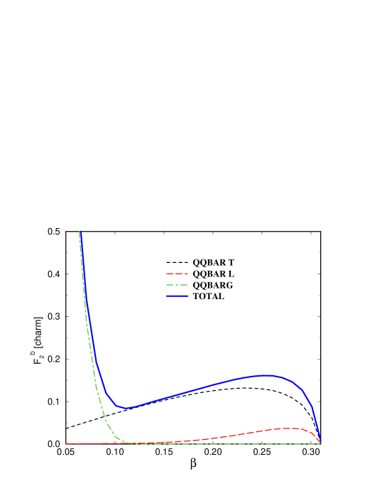
Figure 1: The open charm diffractive structure function and its three components plotted versus $\beta$ for a fixed $x_{{IP}}=0.004$ and $Q^{2}=$ 4 GeV².

In Fig. 1 we present how the three contributions, $c\overline{c}g$, $c\overline{c}$ from transversely and longitudinally polarized photons, contribute for the $\beta$-spectrum of $F_{2}^{D(3)\,\mathrm{charm}}$. At small-$\beta$ we have that the $c\overline{c}g$ component dominates, which implies that the fraction of charm in this regime is predicted to be the same as expected in inclusive charm production ($\approx 25\%$). The above result agree with the theoretical expectations [1]. Since the mass of the quark sets a limit on the size of the $c\overline{c}$ dipole, it becomes color transparent and one expects a strong suppression for this configuration. On the other hand, the effective gluon dipole, associated with $c\overline{c}g$ production is not restricted in size.

Concerning the Regge inspired approaches, diffraction dissociation of virtual photons furnishes the details on the nature of the Pomeron and on its partonic structure. As a first investigation, we follows the Capella-Kaidalov-Merino-Tran Thanh Van (CKMT) model to diffractive DIS based on Regge theory [13, 14] and the Ingelman-Schlein ansatz, which is based on the intuitive picture of a Pomeron flux associated with the proton beam and on the conventional partonic description of the Pomeron-photon collision. In this case, deep inelastic diffractive scattering proceeds in two steps (the Regge factorization): first a Pomeron is emitted from the proton and then the virtual photon is absorbed by a constituent of the Pomeron, in the same way as the partonic structure of the hadrons. In the CKMT model the structure function of the Pomeron, $F_{{IP}}(\beta,Q^{2})$, is associated to the deuteron structure function. The Pomeron is considered as a Regge pole with a trajectory $\alpha_{{IP}}(t)$ determined from soft processes, in which absorptive corrections (Regge cuts) are taken into account. The diffractive contribution to DIS is written in the factorized form,

$$F_{2}^{D(4)}(x_{{IP}},\beta,Q^{2},t)=f(x_{{IP}},t)\,F_{{IP}}\,(\beta,\,Q^{2})\,\,\,,$$ (10)

where the first factor represents the pomeron flux from the proton and can be written as

$$f(x_{{IP}},t)=\frac{[g^{{IP}}_{pp}(t)]^{2}}{16\pi}x_{{IP}}^{1-2\alpha_{{IP}}(t)}\;,$$ (11)

where $g^{{IP}}_{pp}(t)=g^{{IP}}_{pp}(0)\,\exp(C\,t)$ is the Pomeron-proton coupling, with $[g^{{IP}}_{pp}(0)]^{2}=23$ mb and $C=2.2$ GeV^-2 [13, 14]. The Regge factorization implies that the $x_{{IP}}$ dependence is completely separated from the $\beta$ dependence, with the behavior in $x_{{IP}}$ determined only by the flux factor. The value of $\alpha_{{IP}}(t)$ in the flux is given by

$$\alpha_{{IP}}(t)=1+\Delta(Q^{2}_{eff})+\alpha^{\prime}\,t\,\,,$$ (12)

where $\alpha^{\prime}=0.25$ GeV^-2 and

$$\Delta(Q^{2})=\Delta(0)\left(1+\frac{d_{0}\,Q^{2}}{Q^{2}+d_{1}}\right)\,\,,$$ (13)

with $\Delta(0)=0.09663$, $d_{0}=1.9533$ and $d_{1}=1.1606$ [24]. The $Q^{2}$ dependence of the effective Pomeron intercept is one of the main feature of the CKMT model. It was argued in the Refs. [13, 14] that this is due to the fact that the size of the absorptive corrections decreases when $Q^{2}$ increases. This parameterization gives a good description of all existing data on $\gamma^{*}p$ total cross section in the region $Q^{2}\leq 10$ GeV² [24]. At larger $Q^{2}$, effects due to QCD evolution become important. The scale $Q^{2}_{eff}$ is a priori not known. From a theoretical point of view, values for $\Delta(Q^{2}_{eff})$ between 0.13 and 0.24 are possible, corresponding to the effective Pomeron intercept without eikonal-type corrections and the ”bare” value, respectively. Both values are not excluded by the recent fit for the data which assumes in addition to the Pomeron exchange, the contribution of a subleading reggeon trajectory [18, 19]. Integrating Eq. (10) over $t$, $F_{2}^{D(3)}$ can be put in the factorized form

$$F_{2}^{D(3)}(x_{{IP}},\beta,Q^{2})=\overline{f}(x_{{IP}})\,F_{{IP}}\,(\beta,\,Q^{2})\,\,\,,$$ (14)

where $\overline{f}(x_{{IP}})$ is the $t$-integrated pomeron flux

$$\overline{f}(x_{{IP}})=\int_{0}^{\infty}d|t|\,f(x_{{IP}},t)\,\,.$$ (15)

It must be stressed that since the Pomeron is not a particle the separation of the flux factor from the photon-Pomeron cross section is quite arbitrary, and therefore the normalization of the flux is ambiguous.

The second factor in Eq. (10) is the pomeron structure function $F_{{IP}}$ and is proportional to the virtual photon-pomeron cross cross section. In the CKMT approach, $F_{{IP}}(\beta,Q^{2})$ is determined using Regge factorization and the values of the triple Regge couplings determined from soft diffraction data. Namely, the Pomeron structure function is obtained from $F_{2}^{p}$, or more precisely from the combination $F_{2}^{d}=\frac{1}{2}(F_{2}^{p}+F_{2}^{n})$, by replacing the Reggeon-proton couplings by the corresponding triple reggeon couplings (see Ref. [13] for details). The following parametrization of the deuteron structure function $F_{2}^{d}$ at moderate values of $Q^{2}$ (and small-$x$), based on Regge theory, was introduced,

$$F_{2}^{d}(x,Q^{2})=A\,x^{-\Delta(Q^{2})}(1-x)^{n(Q^{2})+4}\left({Q^{2}\over Q^{2}+a}\right)^{1+\Delta(Q^{2})},$$ (16)

where $1+\Delta(Q^{2})$ is the Pomeron intercept, which depends on the photon virtuality. The Pomeron structure function is identical to $F_{2}^{d}$ except for a simple changes in its parameters: $F_{{IP}}(\beta,Q^{2})=F_{2}^{d}\left(x\to\beta;A\to eA,n(Q^{2})\to n(Q^{2})-2\right)$. The value of $e$ in $F_{{IP}}$ is obtained from conventional triple reggeon fits to high mass single diffraction dissociation for soft hadronic processes. The remaining parameters are given in Refs. [13, 14]. In the CKMT approach, the gluon distribution of the Pomeron can be obtained for low $\beta$ in a similar way as for the quarks discussed above. It is written as,

$$\beta\,g_{{IP}}\,(\beta,Q^{2})=e_{d}^{{IP}}\,C_{g}\,\beta^{-\Delta(Q^{2})}\,(1-\beta)^{n_{g}}\,,$$ (17)

where $n_{g}$ is a free parameter and $e_{d}^{{IP}}=r_{{IP}\,{IP}}^{{IP}}(t)/g_{dd}^{{IP}}=0.07$, with $r_{{IP}{IP}}^{{IP}}$ and $g_{dd}^{{IP}}$ being the couplings of the Pomeron to the Pomeron and to the deuteron, respectively. The distribution is singular towards $\beta\to 0$ due to the powerlike behavior driven by the Pomeron exchange. In Ref. [11], where charm diffractive production was computed, $n_{g}$ takes values between 0 and -1 in order to produce a normalizable distribution, which implies for $n_{g}<0$ a singular behavior also at $\beta=1$. As a good description of the $Q^{2}$ dependence of the HERA data is achieved with $n_{g}=0$ and in view that a singular behavior for large $\beta$ is not observed in Regge-like fitting procedures to DDIS data, we assume this value in our analyzes.

In the Regge based approaches, the massive charm contribution arises from photon-gluon fusion. The diffractive structure function is $F_{2}^{D(3)\,\mathrm{charm}}=\overline{f}(x_{{IP}})\times F_{{IP}}^{c\bar{c}}(\beta,Q^{2})$, where $\overline{f}(x_{{IP}})$ is given by Eq. (15) and the charmed contribution to the diffractive Pomeron structure function, $F_{{IP}}^{c\bar{c}}(\beta,Q^{2})$, is given by folding the gluon distribution Eq. (17) in Eq. (6) [11]. The factorization scale is assumed equal to $4\,m_{c}^{2}$. In the general case, the scaling violations of Pomeron structure function should be considered. However, as the $Q^{2}$-range of the HERA data considered here is either small and the parameters in (17) have been obtained for $Q^{2}=5$ GeV², in a first approximation we disregard the logarithmic dependence on $Q^{2}$, which is given by QCD-evolution.

Another possible approach is the QCD analysis of the diffractive structure function in terms of both Regge phenomenology and perturbative QCD evolution as made in Ref. [18]. In this case the parton distributions of the Pomeron are derived from QCD fits of diffrative deep inelastic scattering cross sections determined at HERA. In particular, the diffractive structure functions is given by

$$F_{2}^{D(3)}(Q^{2},\beta,x_{{IP}})=f_{{IP}/p}(x_{{IP}})F_{2}^{{IP}}(Q^{2},\beta)+f_{{IR}/p}(x_{{IP}})F_{2}^{{IR}}(Q^{2},\beta)\,\,,$$ (18)

where $F_{2}^{{IP}}$ can be interpreted as the Pomeron structure function and $F_{2}^{{IR}}$ as an effective Reggeon structure function, with the restriction that it takes into account various secondary Regge contributions which can hardly be separated. The Pomeron and Reggeon fluxes are assumed to follow a Regge behavior with linear trajectories $\alpha_{{IP},{IR}}(t)=\alpha_{{IP},{IR}}(0)+\alpha^{\prime}_{{IP},{IR}}t$, such that

$$f_{{IP}/p,{IR}/p}(x_{{IP}})=\int_{t_{cut}}^{t_{min}}\frac{e^{B_{{IP},{IR}}t}}{x_{{IP}}^{2\alpha_{{IP},{IR}}(t)-1}}dt\,\,,$$ (19)

where $|t_{min}|$ is the minimum kinematically allowed value of $|t|$ and $t_{cut}=-1$ GeV² is the limit of the measurement. The gluon distribution for the Pomeron is parameterized in terms of non-perturbative input distributions at $Q_{0}^{2}=3$ GeV² as follows

$$\beta G(\beta,Q^{2}=Q_{0}^{2})=\left[\sum_{j=1}^{n}C_{j}^{(G)}P_{j}(2z-1)\right]^{2}\,e^{\frac{a}{\beta-1}}\,\,,$$ (20)

and similarly for the quark flavor singlet distribution. The $P_{j}(\eta)$ is the $j^{th}$ member in a set of Chebyshev polynomials, which are chosen such that $P_{1}=1$, $P_{2}=\eta$ and $P_{j+1}=2\eta P_{j}(\eta)-P_{j-1}$. Here we consider this parameterization for the gluon distribution and the corresponding Pomeron flux [Eq. (19)] as input in our calculations. The parameters used are from the H1 fit in Ref.[18].

3 Results and discussion

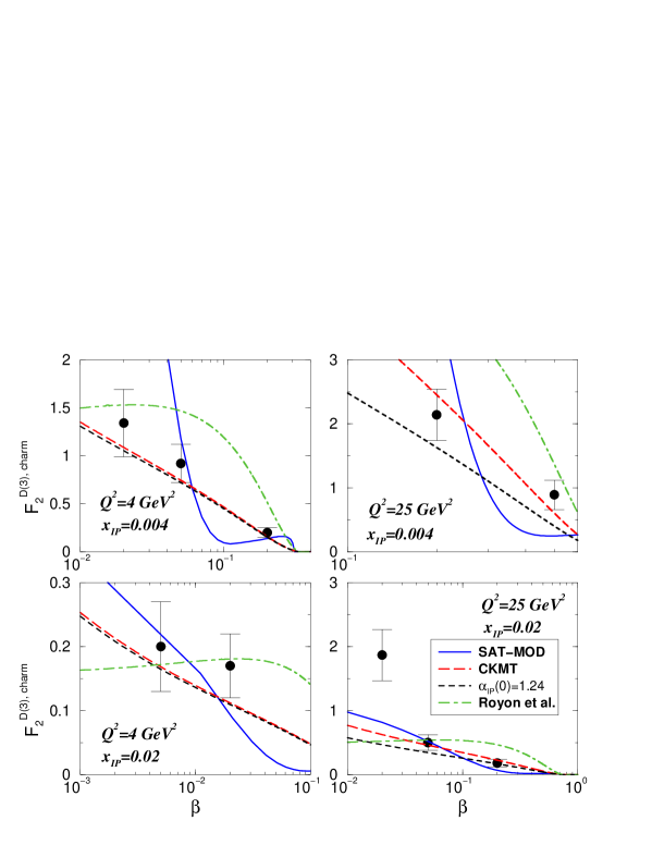
Figure 2: The open charm diffractive structure function $F_{2}^{D(3)\,\mathrm{charm}}$ as a function of $\beta$ (data from ZEUS Collaboration [12]). The solid lines correspond to the perturbative QCD calculation, whereas the other lines represents the results from the Regge approach. The long-dashed curves stand for the CKMT Pomeron and the dashed ones for a fixed Pomeron intercept (see text). The dot-dashed curves represents the result using a Regge/QCD analysis from Ref. [18]

In the previous section, we have reviewed the formulas for the open-charm contribution to the proton diffractive structure functions in the perturbative QCD formalism and Regge based approach. In that follows, one computes the charm diffractive structure function considering these different analysis without additional parameters. In Fig. 2 one presents the results for the QCD approach (solid lines), the CKMT model (dashed and long-dashed lines) and the QCD analysis from Royon et al. [18] (dot-dashed lines) using $m_{c}=1.5$ GeV. In particular, we consider two possibilities for the effective Pomeron intercept $\alpha_{{IP}}(0)=1+\Delta(Q^{2}_{eff})$, which determines the $x_{{IP}}$ dependence of the Pomeron flux. Basically, we have considered the higher ($\alpha_{{IP}}(0)=1.24$) bound obtained in the HERA fit and also an intercept $Q^{2}$-dependent (the CKMT Pomeron).

Regarding the CKMT approach, as the parameters have been constrained for $Q^{2}=5$ GeV², we initially compare our predictions with the experimental results for $Q^{2}=4$ GeV². We have that Regge based approach agrees with ZEUS data both in shape and overall normalization for $Q^{2}$ dependent Pomeron intercept and/or fixed $\alpha_{{IP}}=1.24$. For larger $Q^{2}$ we have that these two choices give different normalizations. However, due to the scarce data a discrimination is still not possible. Moreover, this result can be modified by the QCD evolution, which is not considered in our analyzes. On the other hand, the $\beta$ dependence predicted by the CKMT approach is consistent with the behavior present in the experimental measurements. This result is supported by the phenomenological analyzes from ZEUS [12], which uses a fitting procedure based on QCD factorization for diffractive DIS in order to determine the diffractive quark and gluon distributions.

The result when using the gluon distribution from Ref. [18] is quite different from that one coming from the CKMT model. In particular, the deviation is increasingly larger at small $x_{{IP}}$ and large $Q^{2}$. Moreover, the behavior at small $\beta$ has changed, which becomes flat at this kinematical region. The reason for that is an almost flat diffractive gluon distribution at small $\beta$ coming out of the fit of Ref. [18], whereas one has a singular behavior when considering the CKMT gluon distribution on the Pomeron. These results strongly indicate that the charm diffractive production could allows us further constrain future analysis on the diffractive parton (gluon) distributions on diffractive DIS. It should be noticed a new set of NLO DGLAP/QCD diffractive parton distributions has been recently determined [25] (preliminary), which includes for the first time both experimental and model uncertainties for the error bands of the diffractive pdf’s. There, the small $\beta$ behavior is steep in contrast with the almost flat gluon distribution found in the fit of Ref. [18]. Therefore, it is expected the results using these new parton distributions will modify the analysis presented here.

The perturbative QCD approach provides a steep behavior on $\beta$ in comparison with the Regge based one. In particular, for small $\beta$ and small $x_{{IP}}$ the difference between the predictions is sizeable. The main contribution in the pQCD approach comes from the $c\bar{c}g$ component, which is strongly dependent on the input for the diffractive gluon distribution. Moreover, the implicit dependence on $\beta$ present in the upper limit of the $k_{t}$-integration in Eq. (8) implies an additional $\beta$ dependence. For instance, if we assume in a first approximation that $x_{{IP}}g_{{IP}}(x_{{IP}},k_{t}^{2})\propto\ln k_{t}^{2}$, it would produce a logarithmic enhancement in this dependence. Accordingly, the numerical calculation of Eq. (8) produces a strong growth at small $\beta$ for $x_{{IP}}=0.004$ at both virtualities, either overestimating the data points. However, the description is in agreement with data for $x_{{IP}}=0.02$, even at high $Q^{2}$. It should be noticed that the QCD evolution in the unintegrated gluon distribution may modify this scenario. Furthermore, it is important to emphasize that the pQCD approach predicts a quadratic dependence on $x_{{IP}}g_{{IP}}$. Consequently, for a typical powerlike behavior we expect a stronger dependence than present in the Regge models. Therefore, a better discrimination between the models can be obtained by increasing the data statistics and enlarging the kinematical window.

As a summary, it was shown the diffractive production of open charm is an important observable testing QCD dynamics. The ZEUS collaboration has recently measured [12] the open charm diffractive structure function $F_{2}^{D(3)\,\mathrm{charm}}$, which is extracted from charmed mesons $D^{*\pm}(2010)$ production. The data demonstrate a strong sensitivity to the diffractive parton densities. Here, we have contrasted the pQCD two-gluon exchange approach and Regge/QCD models. For the first one, the saturation model was considered in order to write down the unintegrated gluon distribution. In this case was observed good description at larger $x_{{IP}}$, but a sizeable underestimation at smaller values of $x_{{IP}}$, mostly at smaller $\beta$, is verified. Concerning Regge approach, the CKMT model gives a reasonable data description in shape and normalization with/without a $Q^{2}$-dependent Pomeron intercept. On the other hand, the Regge/QCD approach of Ref. [18] provides a flat behavior at small $\beta$, which is not consistent with the current measurements. A comparison with the most recent parameterizations of diffractive pdf’s is timely. We conclude that an increasingly experimental statistics on this process would help to constrain the diffractive gluon distribution appearing in diffractive factorization approaches and/or discriminate among several parameterizations for the gluon distribution in the Pomeron in approaches based on Regge phenomenology.

References

- [1] M. Wusthoff and A. D. Martin, J. Phys. G 25, R309 (1999).
- [2] A. Hebecker, Phys. Rept. 331, 1 (2000).
- [3] V. Barone and E. Predazzi, High-Energy Particle Diffraction, Springer-Verlag, Berlin Heidelberg, (2002).
- [4] M. B. Gay Ducati, V. P. Goncalves and M. V. T. Machado, Phys. Lett. B 506, 52 (2001).
- [5] M. B. Gay Ducati, V. P. Goncalves and M. V. T. Machado, Nucl. Phys. A 697, 767 (2002).
- [6] S. Munier and A. Shoshi, arXiv:hep-ph/0312022.
- [7] M. Genovese, N. N. Nikolaev and B. G. Zakharov, Phys. Lett. B 378, 347 (1996).
- [8] H. Lotter, Phys. Lett. B 406, 171 (1997).
- [9] E. M. Levin, A. D. Martin, M. G. Ryskin and T. Teubner, Z. Phys. C 74, 671 (1997).
- [10] M. Diehl, Eur. Phys. J. C 1, 293 (1998).
- [11] L. P. A. Haakman, A. B. Kaidalov and J. H. Koch, Eur. Phys. J. C 1, 547 (1998).
- [12] S. Chekanov et al. [ZEUS Collaboration], Nucl. Phys. B 672, 3 (2003).
- [13] A. Capella, A. Kaidalov, C. Merino, D. Pertermann and J. Tran Thanh Van, Phys. Lett. B 343, 403 (1995).
- [14] A. Capella, A. Kaidalov, C. Merino, D. Pertermann and J. Tran Thanh Van, Phys. Rev. D 53, 2309 (1996).
- [15] J. Bartels, J. R. Ellis, H. Kowalski and M. Wusthoff, Eur. Phys. J. C 7, 443 (1999).
- [16] K. Golec-Biernat and M. Wüsthoff, Phys. Rev. D 59, 014017 (1999); ibid. D 60, 114023 (1999); Eur. Phys. J. C 20, 313 (2001).
- [17] S. Munier, R. Peschanski and C. Royon, Nucl. Phys. B 534, 297 (1998).
- [18] C. Royon, L. Schoeffel, J. Bartels, H. Jung and R. Peschanski, Phys. Rev. D 63, 074004 (2001).
- [19] J. Lamouroux, R. Peschanski,C. Royon and L. Schoeffel, Nucl. Phys. B 649, 312 (2003).
- [20] J. C. Collins, Phys. Rev. D 57, 3051 (1998) [Erratum-ibid. D 61, 019902 (2000)].
- [21] V.N. Gribov and L.N. Lipatov, Sov. J. Nucl. Phys. 15, 438 (1972); G. Altarelli and G. Parisi, Nucl. Phys. B 126, 298 (1977); Yu.L. Dokshitzer, Sov. Phys. JETP 46, 641 (1977).
- [22] G. Ingelman and P. E. Schlein, Phys. Lett. B 152, 256 (1985).
- [23] J. Bartels, H. Jung, G. Kyrieleis, Eur. Phys. J. C 24, 555 (2003).
- [24] A. B. Kaidalov, C. Merino and D. Pertermann, Eur. Phys. J. C 20, 301 (2001).
- [25] F. P. Schilling [H1 Collaboration], Acta Phys. Polon. B 33, 3419 (2002) [arXiv:hep-ex/0209001].