Light-cone QCD sum rules for the semileptonic decay $\Lambda_{b}\rightarrow p\ell\bar{\nu}$

Abstract

The exclusive semileptonic heavy baryon decay $\Lambda_{b}\rightarrow p\ell\bar{\nu}$ is investigated using light-cone sum rule method in both full QCD and HQET. The form factors describing the decay are calculated and used to predict the decay width and differential distribution. The total decay width obtained from full QCD is in agreement with the previous theoretical predictions while the HQET result are typically one order smaller. Both results are consistent with the experimental upper limit and can be compared to the refined experimental data in the future.

I Introduction

The study of various decay and formation modes of the $b$ quark is a main source of information about CKM matrix elements and a field for understanding perturbative and nonperturbative QCD effects. In particular, heavy-to-light decays are interesting because they give information on $V_{ub}$, but they are especially difficult to calculate because of the essential presence of strong interactions in the hadronic bound state. The form factors parameterizing the relevant hadronic matrix elements in the heavy-to-light transitions are nonperturbative quantities, which must be estimated in some nonperturbative theoretical approaches. In this regards, the precise calculation of the form factors is provided by lattice simulations. Another fruitful approach has been the application of QCD sum rules on the light-cone BBK ; LCSR ; hqetsum .

The method of light-cone sum rules (LCSR) is a hybrid of the standard technique of QCD sum rules à la SVZ svzsum , with the conventional distribution amplitude description of the hard exclusive process HEP . The basic idea of SVZ sum rules is that using vacuum condensates to parameterize the nontrivial QCD vacuum and employing the duality hypothesis to relate the experimental observable to the theoretical calculation. Technically, operator product expansion (OPE) based on the canonical dimension is used. The difference between SVZ sum rules and LCSR is that the short-distance Wilson OPE in increasing dimension is replaced by the light-cone expansion in terms of distribution amplitudes of increasing twist.

The main nonperturbative parameter in LCSR is the distribution amplitude, also called wave function, which corresponds to the sum of an infinite series of operators with the same twist. In practical application the correlation function considered in LCSR is a $T$ product inserted between physical state and vacuum, which is to be compared to the correlation function between vacuum in the SVZ sum rules. The main contribution to this type of correlation function comes from the light-cone. Using vacuum condensate to characterize the QCD vacuum corresponding to the mean field approximation, and this is valid when the momentum transfer is not so large. When the momentum transfer becomes larger, this approximation cannot be correct everywhere. To this end, the condensates must be replace by the distribution amplitudes, which embodies the fast variation of the field.

Although the LCSR approach does involve a certain model dependence and the leading-order sum rules may not be very accurate, this technique offers an important advantage of being fully consistent with QCD perturbation theory. In recent years there have been numerous applications of LCSR to mesons including the determination of the form factors and the calculations of hadron matrix elements apps ; Btopi ; app-h , see LCSR ; hqetsum for a review. In compliance with the heavy quark symmetry HQET ; review , LCSR within the framework of the Heavy Quark Effective Theory (HQET) has also been formulated and achieved fruitful results. The HQET light-cone sum rules have been applied to deal with the strong couplings of heavy hadrons and heavy-to-light transitions app-hqet .

In this paper we extend the LCSR approach to study the exclusive semileptonic decay $\Lambda_{b}\rightarrow p\ell\bar{\nu}$. Unlike the meson cases, the applications of LCSR to baryons have received little attention because of the lack of knowledge about the distribution amplitudes of higher twists. Recently a comprehensive investigation for the baryonic distribution amplitudes has been given in Ref. hitwist , which makes the calculation of baryon form factors from the LCSR approach feasible. The study for the exclusive semileptonic $\Lambda_{b}$ decay into proton can be found in the literatures by using various approaches such as the SVZ sum rules result1 , the quark model result2 and perturbative QCD factorization theorems pqcd . The existing theoretical predictions vary from each other, and can differ even by orders of magnitude. Here we shall investigate the $\Lambda_{b}\rightarrow p\ell\bar{\nu}$ decay in LCSR and calculate the form factors of the decay within both the framework of full QCD and HQET.

The paper is organized as follows. The full QCD LCSR is derived in Sec. II.1, while the LCSR in HQET is given in Sec. II.2. Sec. III is devoted to the numerical analysis. And in Sec. IV the decay distributions and widths are discussed. Finally, Sec. V is our conclusion. For completeness and convenience we list the nucleon distribution amplitudes in the Appendix.

II $\Lambda_{b}\to p\ell\bar{\nu}$ decay form factors from light-cone sum rules

II.1 LCSR analysis in the full QCD

II.1.1 state of the art: leading twist

In the following LCSR analysis we adopt the current below to interpolate the $\Lambda_{b}$ baryon state

$$j_{\Lambda}=\epsilon_{ijk}(u^{i}C\hbox to0.0pt{/\hss}zd^{j})\gamma_{5}\hbox to0.0pt{/\hss}zb^{k},$$ (1)

where $C$ is the charge conjugation matrix, and $i$, $j$, $k$ denote the color indices. The auxiliary four-vector $z$, which satisfies the light-cone condition $z^{2}=0$, is introduced to project out the main contribution on the light-cone. For the interpolating current used in the sum rule approach, there have been many discussions current . What worth noting is that the current interpolating a given state is not unique, the practical criterion is that the coupling between the interpolating current and the given state must be strong enough. The coupling constant between the interpolating current and the vacuum is

$$\langle 0\mid j_{\Lambda}\mid\Lambda_{b}(P^{\prime})\rangle=f_{\Lambda}z\cdot P^{\prime}\hbox to0.0pt{/\hss}z\,u_{\Lambda},$$ (2)

in which $u_{\Lambda}$ is the $\Lambda_{b}$ baryon spinor and $P^{\prime}$ is the $\Lambda_{b}$ four-momentum.

Our analysis for the decay $\Lambda_{b}\rightarrow p\ell\bar{\nu}$ form factors is analogous to that for the nucleon form factors nucleon . The correlation function we consider in this work is

$$T_{\nu}(P,q)=i\int d^{4}xe^{iq\cdot x}\langle 0\mid T\{j_{\Lambda}(0)j_{\nu}(x)\}\mid P\rangle$$ (3)

where $j_{\nu}=\bar{b}\gamma_{\nu}(1-\gamma_{5})u$ is the weak current. The hadronic matrix element of $j_{\nu}$ inserted between $\Lambda_{b}$ and proton state defines the form factors

$$\langle\Lambda_{b}(P-q)\mid j_{\nu}\mid P\rangle = \bar{u}_{\Lambda}(P-q)\left[f_{1}\gamma_{\nu}-i\frac{f_{2}}{m_{\Lambda}}\sigma_{\nu\mu}q^{\mu}-\frac{f_{3}}{m_{\Lambda}}q_{\nu}\right.$$ (4)

$$- \left.\left(g_{1}\gamma_{\nu}+i\frac{g_{2}}{m_{\Lambda}}\sigma_{\nu\mu}q^{\mu}+\frac{g_{3}}{m_{\Lambda}}q_{\nu}\right)\gamma_{5}\right]N(P),$$

in which $m_{\Lambda}$ is the $\Lambda_{b}$ mass, $N(P)$ denotes the proton spinor and satisfy $\hbox to0.0pt{/\hss}PN(P)=MN(P)$, where $M$ is the proton mass and $P$ is its four-momentum. The six form factors $f_{i}$ and $g_{i}$ are functions of the momentum transfer $q^{2}$. In the case of massless final leptons with $q_{\mu}\bar{\ell}\gamma^{\mu}(1-\gamma_{5})\nu_{\ell}=0$, $f_{3}$ and $g_{3}$ do not contribute. In the following we shall not consider them.

By inserting a complete set of states the correlation function (3) can be represented as

$$z^{\nu}T_{\nu}=\frac{2f_{\Lambda}}{m_{\Lambda}^{2}-P^{\prime 2}}(z\cdot P^{\prime})^{2}\left[f_{1}\hbox to0.0pt{/\hss}z+f_{2}\frac{\hbox to0.0pt{/\hss}z\hbox to0.0pt{/\hss}q}{m_{\Lambda}}-\left(g_{1}\hbox to0.0pt{/\hss}z-g_{2}\frac{\hbox to0.0pt{/\hss}z\hbox to0.0pt{/\hss}q}{m_{\Lambda}}\right)\gamma_{5}\right]N(P)+\cdots,$$ (5)

where $P^{\prime}=P-q$ and the dots stand for the higher resonances and continuum. The contraction with $z^{\nu}$ can simplify the Lorentz structure and remove the $\sim z_{\nu}$ terms which give the subdominant contribution on the light-cone. The form factors enter this expression as the residues of the contribution of ground state $\Lambda_{b}$ baryon.

On the theoretical side, at large Euclidean momenta $P^{\prime 2}$ and $q^{2}$ the correlation function (3) can be calculated in perturbation theory. The diagram contributing to the correlation function is shown in Fig. 1. In the leading order of $\alpha_{s}$ a simple calculation gives

$$z^{\nu}T_{\nu}=-2(C\hbox to0.0pt{/\hss}z)_{\alpha\beta}\hbox to0.0pt{/\hss}z(1-\gamma_{5})_{\mu}\int d^{4}x\int\frac{d^{4}k}{(2\pi)^{4}}\frac{z\cdot k}{k^{2}-m_{b}^{2}}\;e^{i(k+q)\cdot x}\;\langle 0\mid\epsilon_{ijk}u^{i}_{\alpha}(0)u^{j}_{\mu}(x)d^{k}_{\beta}(0)\mid P\rangle\;.$$ (6)

In the light-cone limit $x^{2}\rightarrow 0$, the matrix element of the remaining three quark operators sandwiched between the proton state and vacuum can be parameterized by the leading twist distribution amplitudes HEP ; hitwist ; wf

$$4 \langle 0\mid\epsilon_{ijk}u^{i}_{\alpha}(a_{1}x)u^{j}_{\mu}(a_{2}x)d^{k}_{\beta}(a_{3}x)\mid P\rangle$$ (7)

$$= \mathcal{V}_{1}(\hbox to0.0pt{/\hss}PC)_{\alpha\mu}(\gamma_{5}N)_{\beta}+\mathcal{A}_{1}(\hbox to0.0pt{/\hss}P\gamma_{5}C)_{\alpha\mu}N_{\beta}+\mathcal{T}_{1}(P^{\nu}i\sigma_{\lambda\nu}C)_{\alpha\mu}(\gamma^{\lambda}\gamma_{5}N)_{\beta}.$$

Each distribution amplitudes $\mathcal{V}_{1}$, $\mathcal{A}_{1}$ and $\mathcal{T}_{1}$ can be represented as Fourier integral over the longitudinal momentum fractions $x_{1}$, $x_{2}$, $x_{3}$ carried by the quarks inside the nucleon with $\Sigma_{i}x_{i}=1$,

$$F(a_{k}p\cdot x)=\int\mathcal{D}x\;e^{-ip\cdot x\Sigma_{j}x_{j}a_{j}}F(x_{i}).$$ (8)

The integration measure is defined as

$$\int\mathcal{D}x=\int_{0}^{1}dx_{1}dx_{2}dx_{3}\delta(x_{1}+x_{2}+x_{3}-1).$$ (9)

The normalization of $\mathcal{V}_{1}$ at the origin defines the nucleon coupling constant $f_{N}$,

$$\langle 0\mid\epsilon_{ijk}[u^{i}(0)C\hbox to0.0pt{/\hss}zu^{j}(0)]\gamma_{5}\hbox to0.0pt{/\hss}zd^{k}_{\beta}(0)\mid P\rangle=f_{N}z\cdot P\hbox to0.0pt{/\hss}zN(P).$$ (10)

With these definitions it is easy to obtain the leading twist contribution to Eq. (6),

$$z^{\nu}T_{\nu}=-(z\cdot P)^{2}\int\mathcal{D}x\;x_{2}\frac{V_{1}+A_{1}-2T_{1}}{(x_{2}P-q)^{2}-m_{b}^{2}}\hbox to0.0pt{/\hss}z(1-\gamma_{5})N(P)+\cdots,$$ (11)

where the ellipses stand for contributions that are nonleading in the infinite momentum frame kinematics $P\rightarrow\infty$, $q\sim\mbox{const.}$, $z\sim 1/P$. Note that the light-cone expansion for obtaining Eq. (11) only remains valid at small and intermediate momentum transfer square $q^{2}\leq m_{b}^{2}-O(\Lambda_{\rm QCD}m_{b})$. For larger $q^{2}$ the higher twist contribution will be enhanced and the light-cone expansion becomes meaningless Btopi .

In the leading twist there are only two form factors, $f_{1}$ and $g_{1}$, left. Before proceeding we need the dispersion representation of Eq. (11) for the later use in the matching between the QCD calculation and the hadronic representation in Eq. (5),

$$z^{\nu}T_{\nu}=(P\cdot z)^{2}\int_{m_{b}^{2}}^{\infty}ds\;\frac{\rho(s,Q^{2})}{s-P^{\prime 2}}\;\hbox to0.0pt{/\hss}z(1-\gamma_{5})N(P)+\cdots,$$ (12)

where $Q^{2}=-q^{2}$. If neglecting the terms of $\mathcal{O}(M^{2}/Q^{2})$-which is consistent with twist-$3$ accuracy-such a representation can be easily obtained by substitution $(x_{2}P-q)^{2}-m_{b}^{2}\rightarrow-x_{2}(s-P^{\prime 2})$ with $s=(1-x_{2})Q^{2}/x_{2}+m_{b}^{2}/x_{2}$ in Eq. (11).

In the applications of QCD sum rule method the commonly adopted duality assumption approximates the higher resonances and continuum contributions by the same dispersion integral as that used in Eq. (12) but with the integration variable running above the continuum threshold $s_{0}$. Then the matching between Eqs. (5) and (12) is equivalent to restrict the integration in the dispersion representation below the continuum threshold. This upper bound in $s$ correspond to the lower bound in the momentum fraction: $x_{2}>(Q^{2}+m_{Q}^{2})/(Q^{2}+s_{0})$. Following the standard procedure in QCD sum rule we introduce the Borel transformation to suppress the higher mass contributions

$$-\frac{1}{(x_{2}P-q)^{2}-m_{b}^{2}}=\frac{1}{x_{2}(s-P^{\prime 2})}\rightarrow\frac{1}{x_{2}}exp\left\{-\frac{s}{M_{B}^{2}}\right\}.$$ (13)

Equating the Borel transformed Eq. (5) and Eq. (12) we finally arrives at the sum rule

$$f_{1}^{3}=g_{1}^{3} = \frac{1}{2f_{\Lambda}}\int\mathcal{D}x(V_{1}+A_{1}-2T_{1})exp\left(-\frac{x_{2}Q^{2}-(x_{2}m_{\Lambda}^{2}-m_{b}^{2})}{x_{2}M_{B}^{2}}\right)\Theta\left(x_{2}-\frac{Q^{2}+m_{b}^{2}}{Q^{2}+s_{0}}\right),$$

and $f_{2}^{3}=g_{2}^{3}=0$, where the superscript $3$ denotes the twist-$3$ results. The $\Theta$ function originates from the restriction that the integration of the spectral density must lies within the duality region $s<s_{0}$. In the limit $Q^{2}\rightarrow\infty$ this restriction confines the integration region to $x_{2}\rightarrow 1$. Then it is obvious that the main contribution in this approximation comes from the configuration with a $u$ quark carrying almost the total momentum. And this is precisely the soft, or Feynman mechanism and gives subleading contribution at very large momentum transfer. Indeed using the asymptotic distribution amplitudes $V_{1}(x_{i})=120f_{N}x_{1}x_{2}x_{3}$, $A_{1}(x_{i})=0$ and $T_{1}(x_{i})=V_{1}(x_{i})$, and expanding in powers of $1/Q^{2}$ we find that the sum rule in the $Q^{2}\rightarrow\infty$ limit behaves as

$$f_{1}^{3}=-\frac{10}{Q^{8}}\frac{f_{N}}{f_{\Lambda}}e^{(m_{\Lambda}^{2}-m_{b}^{2})/M_{B}^{2}}\int_{0}^{s_{0}-m_{b}^{2}}dss^{3}e^{-s/M_{B}^{2}},$$ (15)

i.e., it is suppressed by two additional powers of $1/Q^{2}$ compared with the expected asymptotic behavior based on the dimension counting rule. This strong suppression can be compensated by the contributions of the higher twist distribution amplitudes.

II.1.2 beyond the leading twist

Besides the radiative corrections, the higher twist distribution amplitudes do contribute to the correlation function in Eq. (3). There are two kinds of higher twist corrections. One is due to the corrections to the heavy quark propagator in the back ground color field propagator , which correspond to the configuration in the Fock space with a gluon field or quark-antiquark pair in addition to the three valance quarks and give rise to four-particle (and five-particle) nucleon distribution amplitudes. Such effects are usually expected to be small multi-part and we would not take them into account. The other one comes from different Lorentz structures and less singular contributions on the light-cone in the decomposition of the matrix element of the three valance quark operators in Eq. (6), besides those leading twist ones given in Eq. (7). The detailed expression will not be written down here and can be found in hitwist and in the Appendix.

Taking the higher twist distribution amplitudes into account and proceeding as what we have done for the leading twist case, we obtain the following result

$$z^{\nu}T_{\nu} = -(P\cdot z)^{2}\left[\int dx_{2}\;x_{2}\frac{B_{0}(x_{2})}{k^{2}-m_{b}^{2}}-M^{2}\int dx_{3}\;x_{3}\left(\frac{\mathcal{V}_{1}^{M(d)}(x_{3})}{(k^{2}-m_{b}^{2})^{2}}-\frac{2m_{b}^{2}\mathcal{V}_{1}^{M(d)}(x_{3})}{(k^{2}-m_{b}^{2})^{3}}\right)\right.$$ (16)

$$+M^{2}\int dx_{2}\;\frac{x_{2}^{2}B_{1}(x_{2})}{(k^{2}-m_{b}^{2})^{2}}+2M^{2}\int dx_{2}\;x_{2}\left(\frac{B_{2}(x_{2})}{(k^{2}-m_{b}^{2})^{2}}+\frac{2Q^{2}B_{2}(x_{2})}{(k^{2}-m_{b}^{2})^{3}}\right)$$

$$\left.+2M^{4}\int dx_{2}\;\frac{x_{2}^{3}B_{3}(x_{2})}{(k^{2}-m_{b}^{2})^{3}}\right]\hbox to0.0pt{/\hss}z(1-\gamma_{5})N(P)-(P\cdot z)^{2}\left[M\int dx_{2}\;\frac{x_{2}C_{1}(x_{2})}{(k^{2}-m_{b}^{2})^{2}}\right.$$

$$\left.+2M^{3}\int dx_{2}\;\frac{x_{2}^{2}C_{2}(x_{2})}{(k^{2}-m_{b}^{2})^{3}}\right]\hbox to0.0pt{/\hss}z\hbox to0.0pt{/\hss}q(1+\gamma_{5})N(P)+\cdots,$$

where $k=x_{2}P-q$ or $k=x_{3}P-q$, depending on the integral variables, and the functions $B_{i}$, $C_{i}$ are defined by

$$B_{0} = \int_{0}^{1-x_{2}}dx_{1}(V_{1}+A_{1}-2T_{1})(x_{1},x_{2},1-x_{1}-x_{2}),$$

$$B_{1} = -2\tilde{V_{1}}+\tilde{V_{2}}+\tilde{V_{3}}+\tilde{V_{4}}+\tilde{V_{5}}-2\tilde{A_{1}}+\tilde{A_{2}}-\tilde{A_{3}}-\tilde{A_{4}}+\tilde{A_{5}}$$

$$+4\tilde{T_{1}}-2\tilde{T_{2}}-2\tilde{T_{5}}-4\tilde{T_{7}}-4\tilde{T_{8}},$$

$$B_{2} = \tilde{\tilde{T_{2}}}-\tilde{\tilde{T_{3}}}-\tilde{\tilde{T_{4}}}+\tilde{\tilde{T_{5}}}+\tilde{\tilde{T_{7}}}+\tilde{\tilde{T_{8}}},$$

$$B_{3} = \tilde{\tilde{V_{1}}}-\tilde{\tilde{V_{2}}}-\tilde{\tilde{V_{3}}}-\tilde{\tilde{V_{4}}}-\tilde{\tilde{V_{5}}}+\tilde{\tilde{V_{6}}}+\tilde{\tilde{A_{1}}}-\tilde{\tilde{A_{2}}}+\tilde{\tilde{A_{3}}}+\tilde{\tilde{A_{4}}}-\tilde{\tilde{A_{5}}}+\tilde{\tilde{A_{6}}}$$

$$-2(-\tilde{\tilde{T_{1}}}+\tilde{\tilde{T_{2}}}+\tilde{\tilde{T_{5}}}-\tilde{\tilde{T_{6}}}+2\tilde{\tilde{T_{7}}}+2\tilde{\tilde{T_{8}}}),$$

$$C_{1} = \tilde{V_{1}}-\tilde{V_{2}}-\tilde{V_{3}}+\tilde{A_{1}}-\tilde{A_{2}}+\tilde{A_{3}}-2(\tilde{T_{1}}-\tilde{T_{3}}-\tilde{T_{7}}),$$

$$C_{2} = -\tilde{\tilde{V_{1}}}+\tilde{\tilde{V_{2}}}+\tilde{\tilde{V_{3}}}+\tilde{\tilde{V_{4}}}+\tilde{\tilde{V_{5}}}-\tilde{\tilde{V_{6}}}-(\tilde{\tilde{A_{1}}}-\tilde{\tilde{A_{2}}}+\tilde{\tilde{A_{3}}}+\tilde{\tilde{A_{4}}}-\tilde{\tilde{A_{5}}}+\tilde{\tilde{A_{6}}})$$ (17)

$$-2(-\tilde{\tilde{T_{1}}}+\tilde{\tilde{T_{3}}}+\tilde{\tilde{T_{4}}}-\tilde{\tilde{T_{6}}}+\tilde{\tilde{T_{7}}}+\tilde{\tilde{T_{8}}}).$$

The distribution amplitudes with tildes are defined via integrations as follow

$$\tilde{V}(x_{2}) = \int_{1}^{x_{2}}dx^{\prime}_{2}\int_{0}^{1-x^{\prime}_{2}}dx_{1}V(x_{1},x^{\prime}_{2},1-x_{1}-x^{\prime}_{2}),$$

$$\tilde{\tilde{V}}(x_{2}) = \int_{1}^{x_{2}}\int_{1}^{x^{\prime}_{2}}dx^{\prime\prime}_{2}\int_{0}^{1-x^{\prime\prime}_{2}}dx_{1}V(x_{1},x^{\prime\prime}_{2},1-x_{1}-x^{\prime\prime}_{2}).$$ (18)

They originate from the partial integration in order to get rid of the factor $1/P\cdot x$ which appears in the distribution amplitudes. The surface terms for each distribution amplitude sum to zero so they do not contribute. The term $B_{0}$ corresponds to the leading twist contribution, which is given in (11). It is apparent that there arise the form factors $f_{2}$ and $g_{2}$ in (16) due to the higher twist contributions.

The Borel transformation and the continuum subtraction are equivalent to the substitutions below:

$$\int dx\;\frac{\rho(x)}{(k^{2}-m_{b}^{2})^{2}}=\int\frac{dx}{x^{2}}\frac{\rho(x)}{(s^{\prime}-P^{\prime 2})^{2}}\rightarrow\frac{1}{M_{B}^{2}}\int^{1}_{x_{0}}dx\;\frac{\rho(x)}{x^{2}}e^{-s^{\prime}/M_{B}^{2}}+\frac{e^{-s_{0}/M_{B}^{2}}\rho(x_{0})}{Q^{2}+m_{b}^{2}+x_{0}^{2}M^{2}},$$

$$\int dx\;\frac{\rho(x)}{(k^{2}-m_{b}^{2})^{3}}=-\int\frac{dx}{x^{3}}\frac{\rho(x)}{(s^{\prime}-P^{\prime 2})^{3}}\rightarrow-\frac{1}{2M_{B}^{4}}\int^{1}_{x_{0}}dx\;\frac{\rho(x)}{x^{3}}e^{-s^{\prime}/M_{B}^{2}}$$

$$-\frac{e^{-s_{0}/M_{B}^{2}}\rho(x_{0})}{2M_{B}^{2}(Q^{2}+m_{b}^{2}+x_{0}^{2}M^{2})}+\frac{e^{-s_{0}/M_{B}^{2}}x_{0}^{2}}{2(Q^{2}+m_{b}^{2}+x_{0}^{2}M^{2})}\frac{d}{dx_{0}}\left(\frac{\rho(x_{0})}{x_{0}(Q^{2}+m_{b}^{2}+x_{0}^{2}M^{2})}\right),$$ (19)

where

$$s^{\prime}=(1-x)M^{2}+\frac{m_{b}^{2}+(1-x)Q^{2}}{x},$$ (20)

and $x_{0}$ is the positive solution of the quadratic equation for $s^{\prime}=s_{0}$:

$$2M^{2}x_{0}=\sqrt{(Q^{2}+s_{0}-M^{2})^{2}+4M^{2}(Q^{2}+m_{b}^{2})}-(Q^{2}+s_{0}-M^{2}).$$ (21)

Those terms we do not write explicitly in Eq. (II.1.2) give no contributions since all the $\rho(x)$ and the corresponding first order derivative vanishing at $x=1$.

Putting all the results together, it is straightforward to get the final sum rules:

$$-2f_{\Lambda}f_{1}e^{-m_{\Lambda}^{2}/M_{B}^{2}}=-\int_{x_{0}}^{1}dx_{2}\;e^{-s^{\prime}/M_{B}^{2}}\left\{B_{0}+\frac{M^{2}}{M_{B}^{2}}\left[\frac{\mathcal{V}_{1}^{M(d)}(x_{2})}{x_{2}}+\frac{m_{b}^{2}}{M_{B}^{2}}\frac{\mathcal{V}_{1}^{M(d)}(x_{2})}{x_{2}^{2}}\right.\right.$$

$$-B_{1}(x_{2})-2\left.\left.\frac{B_{2}(x_{2})}{x_{2}}-2\frac{Q^{2}}{M_{B}^{2}}\frac{B_{2}(x_{2})}{x_{2}^{2}}+\frac{M^{2}}{M_{B}^{2}}B_{3}(x_{2})\right]\right\}+\frac{M^{2}e^{-s_{0}/M_{B}^{2}}}{m_{b}^{2}+Q^{2}+x_{0}^{2}M^{2}}$$

$$\left[-x_{0}\mathcal{V}_{1}^{M(d)}(x_{0})-\frac{m_{b}^{2}}{M_{B}^{2}}\mathcal{V}_{1}^{M(d)}(x_{0})+x_{0}^{2}B_{1}(x_{0})+2x_{0}B_{2}(x_{0})-2\frac{Q^{2}}{M_{B}^{2}}B_{2}(x_{0})-\frac{M^{2}}{M_{B}^{2}}x_{0}^{2}B_{3}(x_{0})\right]$$

$$+\frac{M^{2}e^{-s_{0}/M_{B}^{2}}x_{0}^{2}}{m_{b}^{2}+Q^{2}+x_{0}^{2}M^{2}}\frac{d}{dx_{0}}\left(\frac{m_{b}^{2}\mathcal{V}_{1}^{M(d)}(x_{0})+2Q^{2}B_{2}(x_{0})+M^{2}x_{0}^{2}B_{3}(x_{0})}{m_{b}^{2}+Q^{2}+x_{0}^{2}M^{2}}\right),$$ (22)

and

$$-2\frac{f_{\Lambda}f_{2}}{Mm_{\Lambda}}e^{-m_{\Lambda}^{2}/M_{B}^{2}}=\frac{1}{M_{B}^{2}}\int_{x_{0}}^{1}\frac{dx_{2}}{x_{2}}\;e^{-s^{\prime}/M_{B}^{2}}\left(C_{1}(x_{2})-\frac{M^{2}}{M_{B}^{2}}C_{2}(x_{2})\right)+\frac{x_{0}e^{-s_{0}/M_{B}^{2}}}{m_{b}^{2}+Q^{2}+x_{0}^{2}M^{2}}$$

$$\left(C_{1}(x_{2})-\frac{M^{2}}{M_{B}^{2}}C_{2}(x_{2})\right)+\frac{M^{2}e^{-s_{0}/M_{B}^{2}}x_{0}^{2}}{m_{b}^{2}+Q^{2}+x_{0}^{2}M^{2}}\frac{d}{dx}\left(\frac{x_{0}C_{2}(x_{0})}{m_{b}^{2}+Q^{2}+x_{0}^{2}M^{2}}\right).$$ (23)

For the sum rules for the form factors $g_{1}$ and $g_{2}$ are identical with those for the $f_{1}$ and $f_{2}$, $f_{1}=g_{1}$ and $f_{2}=g_{2}$, we will only discuss the results for $f_{1}$ and $f_{2}$ in the following sections.

In the above sum rules the four form factors are all functions of the distribution amplitudes. Substituting into the asymptotic distribution amplitudes and expanding in $1/Q^{2}$ we can get the asymptotic behavior of the form factors in the limit $Q^{2}\rightarrow\infty$ as

$$-f_{\Lambda}f_{1}e^{-(m_{\Lambda}^{2}-m_{b}^{2})/M_{B}^{2}} = \frac{M^{2}}{M_{B}^{2}}\frac{f_{N}}{Q^{6}}\int_{0}^{s_{0}-m_{b}^{2}}ds\;e^{-s/M_{B}^{2}}\left[M_{B}^{2}\left(\frac{37}{3}+2\frac{\lambda_{1}}{f_{N}}\right)s-\frac{1}{3}\frac{\lambda_{2}}{f_{N}}s^{2}\right],$$

$$-\frac{f_{\Lambda}f_{2}}{Mm_{\Lambda}}e^{-(m_{\Lambda}^{2}-m_{b}^{2})/M_{B}^{2}} = \frac{f_{N}}{Q^{8}}\int_{0}^{s_{0}-m_{b}^{2}}ds\;e^{-s/M_{B}^{2}}\left[M^{2}(11+\frac{8}{5}\frac{\lambda_{1}}{f_{N}})s+(5+3\frac{\lambda_{1}}{f_{N}})s^{2}\right].$$ (24)

In this limit the order $\mathcal{O}(x^{2})$ correction which is proportional to $\mathcal{V}_{1}^{M(d)}$ goes as $1/Q^{8}$ and gives no contribution to the $f_{1}$ sum rule. It should be noted that we are working with the soft contribution to the form factors. If the hard contribution, which acts as a part of the radiative correction, is taken into account the true asymptotic behavior of $f_{1}$ is expected to be $\sim 1/Q^{4}$, based on the case study of the pion form factors pion .

Unlike the standard QCD sum rule approach, LCSR behaves well under the heavy quark limit. Taking the heavy quark limit in the sum rules is equivalent to the following substitutions app-h ; H-limit :

$$M_{B}^{2}\rightarrow 2m_{b}\tau,\hskip 8.5359pts_{0}\rightarrow m_{b}^{2}+2m_{b}\omega_{0}$$ (25)

Together with the asymptotic distribution amplitudes we obtain the sum rules at the origin in the heavy quark limit

$$-2f_{\Lambda}f_{1}(0)e^{-\bar{\Lambda}/\tau} = \frac{16}{3}\frac{f_{N}}{m_{b}^{4}}\left[60\int_{0}^{\omega_{0}}dss^{3}e^{-s/\tau}-M^{2}\frac{\lambda_{1}}{f_{N}}\int_{0}^{\omega_{0}}dsse^{-s/\tau}\right],$$

$$-2f_{\Lambda}f_{2}(0)e^{-\bar{\Lambda}/\tau} = M\frac{16}{9}\frac{f_{N}}{m_{b}^{3}}(5+3\frac{\lambda_{1}}{f_{N}})\int_{0}^{\omega_{0}}dss^{3}e^{-s/\tau},$$ (26)

where the effective mass $\bar{\Lambda}$ is defined as $\bar{\Lambda}=m_{\Lambda}-m_{b}$.

II.2 LCSR in the HQET

In the HQET we use the following current in the application of LCSR,

$$j_{v}=\epsilon_{ijk}(u^{i}C\hbox to0.0pt{/\hss}zd^{j})\gamma_{5}\hbox to0.0pt{/\hss}zh_{v}^{k},$$ (27)

where the heavy quark field is denoted by $h_{v}$ and $v$ is the heavy quark velocity. The corresponding coupling constant is defined as

$$\langle 0\mid j_{v}\mid\Lambda_{b}(v)\rangle=\hat{f}_{\Lambda}z\cdot v\hbox to0.0pt{/\hss}z\,u_{\Lambda}(v),$$ (28)

in which $u_{\Lambda}$ is the $\Lambda_{b}$ baryon spinor in the HQET. The two form factors for the decay $\Lambda_{b}\rightarrow p\ell\bar{\nu}$ in the HQET are given by the weak matrix element hform

$$\langle\Lambda_{b}(v)\mid j_{\nu}\mid P\rangle=\bar{u}_{\Lambda}(v)\gamma_{\nu}(1-\gamma_{5})(F_{1}+F_{2}\hbox to0.0pt{/\hss}v)N(P).$$ (29)

Both $F_{1}$ and $F_{2}$ are functions of the momentum transfer $\omega=v\cdot P$. The correlation function we consider in this case is

$$T_{\nu}(P,q)=i\int d^{4}xe^{iq\cdot x}\langle 0\mid T\{j_{v}(0)j_{\nu}(x)\}\mid P\rangle.$$ (30)

Then by inserting a complete set of states we obtain the hadronic part of the correlation function as what we have done in order to get the Eq. (5),

$$z^{\nu}T_{\nu}=\frac{\hat{f}_{\Lambda}}{m_{b}}\frac{z\cdot vz\cdot P^{\prime}}{\bar{\Lambda}-\omega^{\prime}}\hbox to0.0pt{/\hss}z(1-\gamma_{5})(F_{1}+F_{2}\hbox to0.0pt{/\hss}v)N(P)+\cdots,$$ (31)

where the variable $\omega^{\prime}$ is defined as $\omega^{\prime}=v\cdot(P-q)=v\cdot P^{\prime}$. It should be remembered that the relevant variable for the dispersion relation is $\omega^{\prime}$ and the consequent Borel transformation is performed on it, too.

The theoretical part can be calculated straightforwardly,

$$z^{\nu}T_{\nu} = z\cdot vz\cdot P\left[\int\frac{\mathcal{D}x}{s^{\prime}-\omega^{\prime}}\left[\frac{K_{1}}{2}-\frac{M^{2}}{4\omega^{2}}K_{2}\right]+\frac{M^{2}}{4}\int dx_{3}\frac{\mathcal{V}_{1}^{M(d)}(x_{3})}{(s^{\prime}-\omega^{\prime})^{3}}\right]\hbox to0.0pt{/\hss}z(1-\gamma_{5})N(P)$$ (32)

$$+ z\cdot vz\cdot P\frac{M}{4\omega}\int\frac{\mathcal{D}x}{s^{\prime}-\omega^{\prime}}H_{1}\hbox to0.0pt{/\hss}z\hbox to0.0pt{/\hss}v(1+\gamma_{5})N(P),$$

where $s^{\prime}=(1-x)\omega$ and the substitution $(xP-q)\cdot v=-(s^{\prime}-\omega^{\prime})$ has been made. The functions $K_{i}$ ($i=1,2$) and $H_{1}$ are defined by

$$K_{1} = V_{1}+A_{1}-2T_{1},$$

$$K_{2} = T_{2}-T_{3}-T_{4}+T_{5}+T_{7}+T_{8},$$

$$H_{1} = -V_{1}+V_{2}+V_{3}-A_{1}+A_{2}-A_{3}+2(T_{1}-T_{3}-T_{7}).$$ (33)

The Borel transformation and continuum subtraction in HQET are performed through substitutions analogous to Eq. (II.1.2),

$$\int dx\;\frac{\rho(x)}{s^{\prime}-\omega^{\prime}} \rightarrow \int dx\rho(x)e^{-s^{\prime}/T}{\Theta}(\omega_{c}-s^{\prime}),$$

$$\int dx\;\frac{\rho(x)}{(s^{\prime}-\omega^{\prime})^{3}} \rightarrow \frac{1}{2T^{2}}\int dx\rho(x)e^{-s^{\prime}/T}{\Theta}(\omega_{c}-s^{\prime})+\frac{e^{-\omega_{c}/T}\rho(x_{c})}{2T\omega}-\frac{e^{-\omega_{c}/T}\rho^{\prime}(x_{c})}{2\omega^{2}},$$

in which $x_{c}=max(0,1-\omega_{c}/\omega)$ and the prime on $\rho$ denotes the derivative. Equating the Borel transformed hadronic part with the theoretical part of the correlation function thus substituted, we arrive at the final sum rules,

$$\frac{\hat{f}_{\Lambda}}{m_{b}}F_{1}(\omega)e^{-\bar{\Lambda}/T} = \int\mathcal{D}xe^{-s^{\prime}/T}\left(\frac{1}{2}K_{1}-\frac{M^{2}}{4\omega^{2}}K_{2}\right)\Theta(\omega_{c}-s^{\prime})+\frac{M^{2}}{8T^{2}}\int_{x_{c}}^{1}dx_{3}\mathcal{V}_{1}^{M(d)}e^{-s^{\prime}/T}$$ (34)

$$+ \frac{M^{2}}{8T\omega}\mathcal{V}_{1}^{M(d)}(x_{c})e^{-\omega_{c}/T}-\frac{M^{2}}{8\omega^{2}}\frac{d}{dx_{c}}\mathcal{V}_{1}^{M(d)}(x_{c})e^{-\omega_{c}/T}$$

and

$$\frac{\hat{f}_{\Lambda}}{m_{b}}F_{2}(\omega)e^{-\bar{\Lambda}/T} = \frac{M}{4\omega}\int\mathcal{D}xH_{1}e^{-s^{\prime}/T}{\Theta}(\omega_{c}-s^{\prime}).$$ (35)

The $K_{1}$ term in Eq. (34) corresponds to the leading twist contribution to the form factor. For the above given sum rules it is obvious that the very soft proton will enhance the higher twist contribution and invalidate the expansion. In practice we will stay away from this region.

For the asymptotic behavior of the form factors in the limit $\omega\rightarrow\infty$, we have

$$\frac{\hat{f}_{\Lambda}}{m_{b}}F_{1}(\omega)e^{-\bar{\Lambda}/T} = \frac{f_{N}}{\omega^{4}}\left[\frac{M^{2}}{12}\left(37+6\frac{\lambda_{1}}{f_{N}}+2\frac{\lambda_{2}}{f_{N}}\right)\delta_{1}(\omega_{c}/T)-\frac{5}{3}\delta_{3}(\omega_{c}/T)\right],$$

$$\frac{\hat{f}_{\Lambda}}{m_{b}}F_{2}(\omega)e^{-\bar{\Lambda}/T} = \frac{f_{N}}{\omega^{3}}\left(5+3\frac{\lambda_{1}}{f_{N}}\right)\delta_{2}(\omega_{c}/T),$$ (36)

where the functions $\delta_{n}$ are defined as

$$\delta_{n}(\omega_{c}/T)=\frac{1}{n!}\int_{0}^{\omega_{c}}dss^{n}e^{-s/T}$$ (37)

and the $\delta_{3}$ term corresponds to the leading twist contribution.

III numerical analysis

In the numerical evaluation, the input parameters can be classified into two parts. One part belongs to the nucleon side, which have been determined before. The other part goes to the $\Lambda_{b}$ baryon sector, which will be given in the following part. Since there have been detailed analysis and discussion about the parameters on the nucleon side in hitwist , we will not dwell on the specific details, but only list the numerical values that will be used in the following analysis,

$$f_{N}=5.3\mathcal{\Theta}10^{-3}\mbox{GeV}^{2},\hskip 8.5359pt\lambda_{1}=-2.7\mathcal{\Theta}10^{-2}\mbox{GeV}^{2},\hskip 8.5359pt\lambda_{2}=5.1\mathcal{\Theta}10^{-2}\mbox{GeV}^{2}.$$ (38)

In the full QCD numerical analysis, we need the coupling constant defined by Eq. (2). In order to get an estimate, we use QCD sum rule method and consider the correlation function

$$\Pi(q^{2})=i\int d^{4}xe^{iq\cdot x}\langle 0\mid T\{j_{\Lambda}(x)\bar{j}_{\Lambda}(0)\}\mid 0\rangle.$$ (39)

The hadronic representation can be obtained immediately

$$\Pi=\frac{2f_{\Lambda}^{2}}{m_{\Lambda}^{2}-q^{2}}(z\cdot q)^{3}\hbox to0.0pt{/\hss}z+\cdots.$$ (40)

On the other hand, the correlation function (39) can be calculated perturbatively in the deep Euclidean region. Then making use of the usual duality assumption and employing Borel transformation to suppress continuum contributions we arrive at the sum rule to dimension $6$ in the OPE

$$2f_{\Lambda}^{2}e^{-m_{\Lambda}^{2}/M_{B}^{2}}=\int_{{m_{b}^{2}}}^{s_{0}}ds\rho(s)e^{-s/M_{B}^{2}},$$ (41)

where the spectral density is

$$\rho(s)=\frac{s}{2^{6}\cdot 5\pi^{4}}\left(1-\frac{m_{b}^{2}}{s}\right)^{5}-\langle\frac{\alpha_{s}}{\pi}G^{2}\rangle\frac{m_{b}^{2}}{2^{5}\cdot 3\pi^{2}s^{2}}\left(1-\frac{m_{b}^{2}}{s}\right)\left(1-\frac{2m_{b}^{2}}{s}\right).$$ (42)

At the working window $38<s_{0}<40\mbox{GeV}^{2}$ and $1<M_{B}^{2}<3\mbox{GeV}^{2}$ the numerical value for the coupling constant reads $f_{\Lambda}=(5\pm 2)\mathcal{\Theta}10^{-3}\mbox{GeV}^{2}$ from (41), where the standard value $\langle\frac{\alpha_{s}}{\pi}G^{2}\rangle=0.012~{}\mbox{GeV}^{2}$ is adopted.

In the numerical calculations for the form factors, $f_{1}$ and $f_{2}$, the center values we take for the heavy quark mass and the continuum threshold are $m_{b}=4.8~{}\mbox{GeV}$ mb-lb and $s_{0}=39~{}\mbox{GeV}^{2}$ excited-mass , and the $\Lambda_{b}$ baryon mass can be found in PDG2002 . Then substitute into the explicit form of $f_{\Lambda}$ and vary the continuum threshold in the range $s_{0}=38-40~{}\mbox{GeV}^{2}$, we find that the stability is acceptable in $M_{B}^{2}=6-9~{}\mbox{GeV}^{2}$ for the Borel parameter. The $M_{B}^{2}$ and the $q^{2}$ dependence for the form factors are shown in Figs. 2 and 3, respectively.

Both the form factors in a subrange of the whole kinematical region, which depends on the heavy quark mass, can be fitted well by the dipole formula

$$f_{i}(q^{2})=\frac{f_{i}(0)}{a_{2}(q^{2}/m_{\Lambda}^{2})^{2}+a_{1}q^{2}/m_{\Lambda}^{2}+1}.$$ (43)

But the whole kinematical fit is not satisfactory. Below corresponding to the asymptotic and QCD sum rule obtained distribution amplitudes we give the coefficients for a special set of values in Table 1, for which the largest uncertainty occurs in the end-point region $q^{2}\sim 16~{}\mbox{GeV}^{2}$ and is less than $10\%$.

	asymptotic						QCD sum rule
	$a_{2}$		$a_{1}$		$f_{i}(0)$		$a_{2}$		$a_{1}$		$f_{i}(0)$
$f_{1}$	$2$.	$381$	$-2$.	$888$	$-0$.	$037$	$5$.	$590$	$-2$.	$759$	$0$.	$018$
$f_{2}$	$2$.	$582$	$-3$.	$026$	$0$.	$027$	$2$.	$000$	$-2$.	$603$	$0$.	$159$

Table 1: The dipole fit for the form factors $f_{1}$ and $f_{2}$ in the subregion $0<q^{2}<16~{}\mbox{GeV}^{2}$ with $M_{B}^{2}=8~{}\mbox{GeV}^{2}$, $s_{0}=39~{}\mbox{GeV}^{2}$ and $m_{b}=4.8~{}\mbox{GeV}$.

As already mentioned above in section II.1, the light-cone expansion is expected to hold only at $q^{2}\leq m_{b}^{2}-O(\Lambda_{\rm QCD}m_{b})\approx 17$ ${\rm GeV}^{2}$. In fact, the fast increase of the form factors in Figs. 2 and 3 near the end-point region indicates that when the momentum transfer is large or $q^{2}$ approaches the kinematical limit, the dispersion represented integral in (11) tends to grow strongly and cannot be enough suppressed by Borel transformation in the subsequently obtained sum rules. This can also be substantiated by the dipole fit procedure: If the formula (43) is used for the fit, then there exists no satisfactory fit for the form factors in the whole range of the kinematical region and the uncertainty near the end-point region is large, which can even amount to $80\%$. Taking into account this fact, we are satisfied to fit the form factors in a subregion of the whole kinematical region, just as what we have done in Table 1, and then extrapolate to get the behavior near the end-point.

The numerical analysis in the HQET goes parallel with that in the full QCD. What we consider first is sum rule for the coupling constant, and the vacuum-to-vacuum correlation function is

$$\Pi(q^{2})=i\int d^{4}xe^{iq\cdot x}\langle 0\mid T\{j_{v}(x)\bar{j}_{v}(0)\}\mid 0\rangle.$$ (44)

The phenomenological part can be obtained by inserting a complete set of states

$$\Pi=\frac{\hat{f}_{\Lambda}^{2}}{\bar{\Lambda}-\omega}(z\cdot v)^{3}\hbox to0.0pt{/\hss}z+\cdots,$$ (45)

where $\omega=v\cdot q$. The theoretical calculation is straightforward. After the Borel transformation and continuum subtraction we get the final sum rule

$$\hat{f}_{\Lambda}^{2}e^{-\bar{\Lambda}/T}=\frac{1}{10\pi^{4}}\int_{0}^{\omega_{c}}d\omega\omega^{5}e^{-\omega/T}+\frac{T^{2}}{3\cdot 2^{4}\pi^{2}}\langle\frac{\alpha_{s}}{\pi}G^{2}\rangle.$$ (46)

Vary the parameters in the range $0.1<T<0.5\mbox{GeV}$, $1.6<\omega_{c}<1.8\mbox{GeV}$, we arrive at the following value for the coupling constant in the HQET $\hat{f}_{\Lambda}=(2.9\pm 1.0)\mathcal{\Theta}10^{-2}\mbox{GeV}^{3}$, where the effective mass is taken to be $\bar{\Lambda}=0.8\mbox{GeV}$.

As what have been done in the full QCD, in the HQET analysis we substitute the explicit form for $\hat{f}_{\Lambda}$ into the numerical analysis. We work with the following parameters for the continuum threshold $\omega_{c}$ and the Borel parameter $T$ in the HQET light-cone sum rules

$$\omega_{c}=1.6-1.8\mbox{GeV},\hskip 8.5359ptT=0.8-1.2\mbox{GeV}.$$ (47)

The stability in the above given region is satisfactory. In Figs. 4 and 5 we show the dependence of $F_{1}$ and $F_{2}$ on Borel parameter $T$ and momentum transfer $\omega$. The overall behavior of the form factors $F_{1}$ and $F_{2}$ cannot be fitted well by simple functions, but for large $\omega$, say $\omega>\omega_{c}$, the following formula fits them well,

$$F_{i}(\omega)=a_{0}+a_{1}\omega+a_{2}\omega^{2}.$$ (48)

This is due to the fact that the higher twist contributions will be enhanced by the small $\omega$, just as mentioned above in Sec. II.2. What given in Table 2 is our fit for the center value of the effective mass $\bar{\Lambda}=0.8\mbox{GeV}$, corresponding to the asymptotic and QCD sum rule obtained distribution amplitudes.

	asymptotic						QCD sum rule
	$a_{2}$		$a_{1}$		$a_{0}$		$a_{2}$		$a_{1}$		$a_{0}$
$F_{1}$	$-0$.	$073$	$0$.	$471$	$-0$.	$802$	$-0$.	$141$	$0$.	$802$	$-1$.	$142$
$F_{2}$	$-0$.	$003$	$0$.	$044$	$-0$.	$124$	$0$.	$054$	$-0$.	$238$	$0$.	$153$

Table 2: The fit performed in the region $\omega>2.0\mbox{GeV}$ for the form factors $F_{1}$ and $F_{2}$ with $\bar{\Lambda}=0.8\mbox{GeV}$, $\omega_{c}=1.7\mbox{GeV}$ and $T=1\mbox{GeV}$.

Based on similar reasoning, it is obvious that the bizarre behavior of the form factors in the small $\omega$ region is due to the not enough suppression $1/(x_{2}P-q)\cdot v$ in (32) when $\omega$ is not large enough. In order to dodge this region we just follow the same tactic as used in the full QCD case and fit the form factors for the large $\omega$ region, which is exactly what we have done above.

Due to the numerically large values $\lambda_{1}/f_{N}=-5.1\pm 1.7$ and $\lambda_{2}/f_{N}=9.6\pm 3.6$, it is expected that the twist-$4$ contribution will be large as compared to the leading twist-$3$ contribution. We find that it indeed is the case in our calculation, which can be seen more clearly in the asymptotic sum rules (24) and (36). In the full QCD, the twist-$4$ and twist-$5$ contributions amount to approximately $30\%$ and $80\%$ for the form factor $f_{1}$, respectively; while for the form factor $f_{2}$, the twist-$4$ contribution is almost the same in magnitude as the leading twist-$3$ one, at the same time the twist-$5$ contribution is small, less than $1\%$, thus negligible. The case is similar for both the QCD sum rule obtained and asymptotic distribution amplitudes. When approaching the end-point $q^{2}\sim 22\mbox{GeV}^{2}$, the twist-$4$ and $5$ contributions for $f_{1}$ increase, but they have opposite sings and thus tend to cancel each other and the net contribution is only $\sim 30\%$ or $\sim 100\%$ to that of twist-$3$ distribution amplitudes, corresponding to the asymptotic or sum rule obtained distribution amplitudes; for $f_{2}$, the higher twist contributions decrease and are negligible near the end-point region. The HQET case is not so good. For $F_{1}$, when $\omega$ is small, the twist-$5$ contribution is small and well under control. But when $\omega$ gets larger, the twist-$5$ contribution tends to surpass the leading twist-$3$ part and becomes the dominant one for the sum rule obtained distribution amplitudes when the Borel parameter $T$ is not large enough, while for the asymptotic distribution amplitudes, the twist-$5$ contribution remains small, $\sim 20\%$, in the whole kinematical region. The twist-$4$ contribution is small for two kind distribution amplitudes, less than $10\%$, and the twist-$6$ contribution is zero. However, the twist-$4$ contribution is expected to be large and the combination of the twist-$3$ and $4$ contributions should be the dominant one, thus the smallness of the twist-$4$ contribution, which results from the missing of the twist-$4$ distribution amplitudes in the $F_{1}$ sum rule, is not acceptable. But as a compromise, the twist-$5$ contribution is also small and the leading twist-$3$ contribution is the dominant one. For $F_{2}$, the twist-$4$ contribution is larger than the twist-$3$ one. And there is no twist-$5$ contribution for $F_{1}$ and twist-$6$ contribution for both $F_{1}$ and $F_{2}$. If we take the sum of twist-$3$ and $4$ contributions as the dominant one, then the higher twist contribution is exactly zero in our calculation. What should be noted is that the inclusion of twist-$6$ contribution in our calculation is not complete, the only one included serves as an estimate of order. For all the cases it is small, less than $1\%$, and can be neglected. This may be seen as an indication that our results are not sensitive to the still higher twist contributions. Besides, the main uncertainty in our numerical analysis comes from the uncertainties in $f_{N}$, $\lambda_{1}$ and $\lambda_{2}$, this can lead to a $\sim 30\%$ uncertainty for the form factors.

IV Semileptonic decay distributions and widths

For the decay $\Lambda_{b}\rightarrow p\ell\bar{\nu}$ in the full QCD, the kinematical region is $0<q^{2}<(m_{\Lambda}-M)^{2}$, which is available from the LCSR in this work, though the end-point behavior may be unreliable. For this end-point region is marginal and thus has moderate effect for the total decay width. The differential decay rate can be expressed as

$$\frac{d\Gamma}{dq^{2}} = \frac{G_{F}^{2}|V_{ub}|^{2}}{192\pi^{3}m_{\Lambda}^{5}}q^{2}\sqrt{q_{+}^{2}q_{-}^{2}}[-6f_{1}f_{2}m_{\Lambda}m_{+}q_{-}^{2}+6g_{1}g_{2}m_{\Lambda}m_{-}q_{+}^{2}$$ (49)

$$+ f_{1}^{2}m_{\Lambda}^{2}[\frac{m_{+}^{2}m_{-}^{2}}{q^{2}}+m_{-}^{2}-2(q^{2}+2m_{\Lambda}M)]+g_{1}^{2}m_{\Lambda}^{2}[\frac{m_{+}^{2}m_{-}^{2}}{q^{2}}+m_{+}^{2}-2(q^{2}-2m_{\Lambda}M)]$$

$$- g_{2}^{2}[-2m_{+}^{2}m_{-}^{2}+m_{-}^{2}q^{2}+q^{2}(q^{2}-4Mm_{\Lambda})]-f_{2}^{2}[-2m_{+}^{2}m_{-}^{2}+m_{+}^{2}q^{2}+q^{2}(q^{2}+4Mm_{\Lambda})]]$$

where $m_{\pm}=m_{\Lambda}\pm M$ and $q^{2}_{\pm}=q^{2}-m^{2}_{\pm}$. Using the form factors given in Eqs. (II.1.2) and (II.1.2), and the $\Lambda_{b}$ and proton masses PDG2002 , we can compute the differential decay rate and the total decay width. The differential decay rate is shown in Fig. 6. The total decay widths after the integration over the whole range of $q^{2}$ are given in Table 3, corresponding to the asymptotic and sum rule obtained distribution amplitudes. The effect of the heavy quark mass is also taken into account here. There is no apparent distinction between the two kind of results, and within each kind the dependence on the heavy quark mass is mild. The referred error is due to the variation of the Borel parameter and the continuum threshold only. What should be remarked here is that the value $m_{b}=4.7\mbox{GeV}$ lies on the margin of the possible region in which the whole range of the kinematical $q^{2}$ can be accessed. Due to the radical increase of the form factors near the end-point, one may suspects the reliability of the sum rule prediction in that region, just as mentioned above in Sec. III. So correspondingly, the total decay widths using the fitted form factors are also given in Table 3. The difference is not drastic. Our results given in Table 3 are in agreement with the QCD sum rule predictions both in the full QCD and HQET result1 .

	asymptotic			QCD sum rule
$m_{b}(\mbox{GeV})$	$4.7$	$4.8$	$4.9$	$4.7$	$4.8$	$4.9$
$\Gamma$	$1.5\pm 0.7$	$1.0\pm 0.4$	$0.7\pm 0.2$	$3.7\pm 2.2$	$3.1\pm 1.8$	$2.6\pm 1.4$
$\Gamma_{f}$	$0.56\pm 0.14$	$0.44\pm 0.09$	$0.35\pm 0.06$	$2.4\pm 1.3$	$2.0\pm 1.0$	$1.7\pm 0.8$

Table 3: Decay widths $(\mbox{in}\,10^{-11}\times|V_{ub}|^{2}\,\mbox{\mbox{GeV}})$ for the semileptonic decays $\Lambda_{b}\rightarrow p\ell\bar{\nu}$. $\Gamma$ is obtained by integrating in the whole kinematical region using sum rule data, while $\Gamma_{f}$ using the $q^{2}<16\mbox{GeV}^{2}$ fitted form factors extrapolated to the whole region. The error only reflects the variation of the Borel parameter and the continuum threshold between $6<M_{B}^{2}<9\mbox{GeV}^{2}$ and $38<s_{0}<40\mbox{GeV}^{2}$.

The differential decay rate for the decay $\Lambda_{b}\rightarrow p\ell\bar{\nu}$ in HQET is

$$\frac{d\Gamma}{d\omega} = \frac{G_{F}^{2}|V_{ub}|^{2}}{12\pi^{3}}[F_{1}^{2}(3m_{\Lambda}^{2}\omega+3M^{2}\omega-2m_{\Lambda}(M^{2}+2\omega^{2}))+2F_{1}F_{2}M(3m_{\Lambda}^{2}+M^{2}$$ (50)

$$- 6m_{\Lambda}\omega+2\omega^{2})+F_{2}^{2}(3m_{\Lambda}^{2}\omega-M^{2}\omega+4\omega^{3}+2m_{\Lambda}(M^{2}-4\omega^{2}))]\sqrt{\omega^{2}-M^{2}},$$

where the kinematical region for $\omega$ is $M<\omega<\omega_{max}=(m_{\Lambda}^{2}+M^{2})/2m_{\Lambda}$. Taking into the form factors given by sum rules in Eqs. (34) and (35) we can obtain the differential decay rate $d\Gamma/d\omega$ and the total decay width $\Gamma$. The differential decay rate is shown in Fig. 7 and the total decay widths are given in Table 4. Based on similar consideration, the total decay widths corresponding to the fitted form factors are also given in Table 4. The results are almost the same. Compared to the full QCD result, the decay width in HQET is typically one order smaller for the sum rule obtained distribution amplitudes. As for the asymptotic results, the decay width is almost the same in magnitude. Our QCD sum rule obtained results in the HQET are comparable to those in result2 .

	asymptotic			QCD sum rule
$\bar{\Lambda}(\mbox{GeV})$	$0.7$	$0.8$	$0.9$	$0.7$	$0.8$	$0.9$
$\Gamma$	$2.8\pm 0.7$	$3.0\pm 0.8$	$3.2\pm 0.9$	$2.9\pm 1.0$	$3.1\pm 1.1$	$3.4\pm 1.3$
$\Gamma_{f}$	$3.5\pm 0.7$	$3.7\pm 0.8$	$4.0\pm 0.9$	$3.4\pm 0.5$	$3.6\pm 0.6$	$3.9\pm 0.8$

Table 4: Decay widths $(\mbox{in}\,10^{-12}\times|V_{ub}|^{2}\,\mbox{\mbox{GeV}})$ for the semileptonic decays $\Lambda_{b}\rightarrow p\ell\bar{\nu}$ in HQET. $\Gamma$ denotes the total decay width using sum rules for $F_{1}$ and $F_{2}$, and $\Gamma_{f}$ using the form factors fitted in $\omega>2.0\mbox{GeV}$ then extrapolated to the whole region. The averages are taken between $0.8<T<1.2\mbox{GeV}$, $1.6<\omega_{c}<1.8\mbox{GeV}$.

V Conclusion

In conclusion, we have investigated the semileptonic decay $\Lambda_{b}\rightarrow p\ell\bar{\nu}$ using the light-cone sum rule method both in the full QCD and the HQET. The form factors parameterizing the weak matrix elements of the decay are calculated with asymptotic and QCD sum rule obtained distribution amplitudes and used to predict the decay width and differential distribution. For the numerical results, we find that the total decay widths given in the full QCD are in agreement with previous theoretical works and not inconsistent with the experimental upper limit. However, the total decay widths with sum rule obtained distribution amplitudes in the HQET are typically one order smaller than those in the full QCD. What remarkable here is that the asymptotic HQET and full QCD results are almost the same with the fitted form factors, cf. Tables 3 and 4. As for the physical behavior of the distribution amplitudes, the current experimental data is not enough to discriminate which one, between the asymptotic and the QCD sum rule obtained, is correct in this kinematical region, because the total decay widths corresponding to different distribution amplitudes do not deviate from each other greatly, though the predicted behaviors for the form factors are completely different. Moreover, the $\mathcal{O}(\alpha_{s})$ correction to the LCSR, which amounts to the hard gluon exchange mechanism, is needed as a complete description for the decay in the full QCD. As to the HQET case, our results are merely preliminary and further improvements, which including order $\bar{\Lambda}_{QCD}/m_{Q}$ corrections in the heavy quark expansion and radiative corrections, are needed to reconcile the existing discrepancy between the HQET and full QCD results. Finally, it is worth remarking that the light-cone expansion for the correlation function is not accessible at all momentum transfers. The restriction on $q^{2}$ is in the region $q^{2}\leq m_{b}^{2}-O(\Lambda_{\rm QCD}m_{b})\approx 17{\rm GeV}^{2}$. When $q^{2}$ becomes large or one gets too close to the physical states in the channel, light-cone expansion tends to break down. So the LCSR in the large $q^{2}$ region may be not reliable and cannot give much information on the physical behavior or the form factors. The HQET case is similar, the only difference is that the expansion parameter is $\omega$ and correspondingly the restriction turns to be the lower limit of $\omega$, thus soft proton will enhance the higher twist contributions.

Appendix: The nucleon distribution amplitudes with $O(x^{2})$ corrections

The nucleon distribution amplitudes are defined by matrix element

$$4\langle 0|\epsilon^{ijk}u_{\alpha}^{i}(a_{1}x)u_{\beta}^{j}(a_{2}x)u_{\gamma}^{k}(a_{3}x)|P\rangle=\mathcal{S}_{1}MC_{\alpha\beta}(\gamma_{5}N)_{\gamma}+\mathcal{S}_{2}M^{2}C_{\alpha\beta}(\hbox to0.0pt{/\hss}x\gamma_{5}N)_{\gamma}$$

$${}+\mathcal{P}_{1}M(\gamma_{5}C)_{\alpha\beta}N_{\gamma}+\mathcal{P}_{2}M^{2}(\gamma_{5}C)_{\alpha\beta}(\hbox to0.0pt{/\hss}xN)_{\gamma}+(\mathcal{V}_{1}+\frac{x^{2}M^{2}}{4}\mathcal{V}_{1}^{M})(\hbox to0.0pt{/\hss}PC)_{\alpha\beta}(\gamma_{5}N)_{\gamma}$$

$${}+\mathcal{V}_{2}M(\hbox to0.0pt{/\hss}PC)_{\alpha\beta}(\hbox to0.0pt{/\hss}x\gamma_{5}N)_{\gamma}+\mathcal{V}_{3}M(\gamma_{\mu}C)_{\alpha\beta}(\gamma^{\mu}\gamma_{5}N)_{\gamma}+\mathcal{V}_{4}M^{2}(\hbox to0.0pt{/\hss}xC)_{\alpha\beta}(\gamma_{5}N)_{\gamma}$$

$${}+\mathcal{V}_{5}M^{2}(\gamma_{\mu}C)_{\alpha\beta}(i\sigma^{\mu\nu}x_{\nu}\gamma_{5}N)_{\gamma}+\mathcal{V}_{6}M^{3}(\hbox to0.0pt{/\hss}xC)_{\alpha\beta}(\hbox to0.0pt{/\hss}x\gamma_{5}N)_{\gamma}$$

$${}+(\mathcal{A}_{1}+\frac{x^{2}M^{2}}{4}\mathcal{A}_{1}^{M})(\hbox to0.0pt{/\hss}P\gamma_{5}C)_{\alpha\beta}N_{\gamma}+\mathcal{A}_{2}M(\hbox to0.0pt{/\hss}P\gamma_{5}C)_{\alpha\beta}(\hbox to0.0pt{/\hss}xN)_{\gamma}+\mathcal{A}_{3}M(\gamma_{\mu}\gamma_{5}C)_{\alpha\beta}(\gamma^{\mu}N)_{\gamma}$$

$${}+\mathcal{A}_{4}M^{2}(\hbox to0.0pt{/\hss}x\gamma_{5}C)_{\alpha\beta}N_{\gamma}+\mathcal{A}_{5}M^{2}(\gamma_{\mu}\gamma_{5}C)_{\alpha\beta}(i\sigma^{\mu\nu}x_{\nu}N)_{\gamma}+\mathcal{A}_{6}M^{3}(\hbox to0.0pt{/\hss}x\gamma_{5}C)_{\alpha\beta}(\hbox to0.0pt{/\hss}xN)_{\gamma}$$

$${}+(\mathcal{T}_{1}+\frac{x^{2}M^{2}}{4}\mathcal{T}_{1}^{M})(P^{\nu}i\sigma_{\mu\nu}C)_{\alpha\beta}(\gamma^{\mu}\gamma_{5}N)_{\gamma}+\mathcal{T}_{2}M(x^{\mu}P^{\nu}i\sigma_{\mu\nu}C)_{\alpha\beta}(\gamma_{5}N)_{\gamma}$$

$${}+\mathcal{T}_{3}M(\sigma_{\mu\nu}C)_{\alpha\beta}(\sigma^{\mu\nu}\gamma_{5}N)_{\gamma}+\mathcal{T}_{4}M(P^{\nu}\sigma_{\mu\nu}C)_{\alpha\beta}(\sigma^{\mu\rho}x_{\rho}\gamma_{5}N)_{\gamma}$$

$${}+\mathcal{T}_{5}M^{2}(x^{\nu}i\sigma_{\mu\nu}C)_{\alpha\beta}(\gamma^{\mu}\gamma_{5}N)_{\gamma}+\mathcal{T}_{6}M^{2}(x^{\mu}P^{\nu}i\sigma_{\mu\nu}C)_{\alpha\beta}(\hbox to0.0pt{/\hss}x\gamma_{5}N)_{\gamma}$$

$${}+\mathcal{T}_{7}M^{2}(\sigma_{\mu\nu}C)_{\alpha\beta}(\sigma^{\mu\nu}\hbox to0.0pt{/\hss}x\gamma_{5}N)_{\gamma}+\mathcal{T}_{8}M^{3}(x^{\nu}\sigma_{\mu\nu}C)_{\alpha\beta}(\sigma^{\mu\rho}x_{\rho}\gamma_{5}N)_{\gamma}.$$ (51)

The calligraphic distribution amplitudes do not have definite twist, but can be related to the ones with definite twist as

$$\mathcal{S}_{1}=S_{1},\hskip 22.76228pt2P\cdot x\mathcal{S}_{2}=S_{1}-S_{2},$$

$$\mathcal{P}_{1}=P_{1},\hskip 22.76228pt2P\cdot x\mathcal{P}_{2}=P_{1}-P_{2}$$ (52)

for the scalar and pseudo-scalar distributions,

$$\mathcal{V}_{1}=V_{1},\hskip 68.28644pt2P\cdot x\mathcal{V}_{2}=V_{1}-V_{2}-V_{3},$$

$$2\mathcal{V}_{3}=V_{3},\hskip 62.59596pt4P\cdot x\mathcal{V}_{4}=-2V_{1}+V_{3}+V_{4}+2V_{5},$$

$$4P\cdot x\mathcal{V}_{5}=V_{4}-V_{3},\hskip 14.22636pt(2P\cdot x)^{2}\mathcal{V}_{6}=-V_{1}+V_{2}+V_{3}+V_{4}+V_{5}-V_{6}$$ (53)

for the vector distributions,

$$\mathcal{A}_{1}=A_{1},\hskip 68.28644pt2P\cdot x\mathcal{A}_{2}=-A_{1}+A_{2}-A_{3},$$

$$2\mathcal{A}_{3}=A_{3},\hskip 62.59596pt4P\cdot x\mathcal{A}_{4}=-2A_{1}-A_{3}-A_{4}+2A_{5},$$

$$4P\cdot x\mathcal{A}_{5}=A_{3}-A_{4},\hskip 14.22636pt(2P\cdot x)^{2}\mathcal{A}_{6}=A_{1}-A_{2}+A_{3}+A_{4}-A_{5}+A_{6}$$ (54)

for the axial vector distributions, and

$$\mathcal{T}_{1}=T_{1},\hskip 109.54327pt2P\cdot x\mathcal{T}_{2}=T_{1}+T_{2}-2T_{3},$$

$$2\mathcal{T}_{3}=T_{7},\hskip 104.70593pt4P\cdot x\mathcal{T}_{4}=T_{1}-T_{2}-2T_{5},$$

$$4P\cdot x\mathcal{T}_{5}=-T_{1}+T_{5}+2T_{8},\hskip 14.22636pt(2P\cdot x)^{2}\mathcal{T}_{6}=2T_{2}-3T_{3}-2T_{4}+2T_{5}+2T_{7}+2T_{8},$$

$$4P\cdot x\mathcal{T}_{7}=T_{7}-T_{8},\hskip 54.06006pt(2P\cdot x)^{2}\mathcal{T}_{8}=-T_{1}+T_{2}+T_{5}-T_{6}+2T_{7}+2T_{8}$$ (55)

for the tensor distributions. Each distribution amplitudes $F=V_{i},A_{i},T_{i},S_{i},P_{i}$ can be represented as

$$F(a_{i}p\cdot x)=\int\mathcal{D}xe^{-ip\cdot x\Sigma_{i}x_{i}a_{i}}F(x_{i})\;.$$ (56)

Those distribution amplitudes are scale dependent and can be expanded in contributions of conformal operators. To the next-to-leading conformal spin accuracy the expansion reads hitwist

$$V_{1}(x_{i},\mu) = 120x_{1}x_{2}x_{3}[\phi_{3}^{0}(\mu)+\phi_{3}^{+}(\mu)(1-3x_{3})],$$

$$V_{2}(x_{i},\mu) = 24x_{1}x_{2}[\phi_{4}^{0}(\mu)+\phi_{3}^{+}(\mu)(1-5x_{3})],$$

$$V_{3}(x_{i},\mu) = 12x_{3}\{\psi_{4}^{0}(\mu)(1-x_{3})+\psi_{4}^{-}(\mu)[x_{1}^{2}+x_{2}^{2}-x_{3}(1-x_{3})]$$

$$+ \psi_{4}^{+}(\mu)(1-x_{3}-10x_{1}x_{2})\},$$

$$V_{4}(x_{i},\mu) = 3\{\psi_{5}^{0}(\mu)(1-x_{3})+\psi_{5}^{-}(\mu)[2x_{1}x_{2}-x_{3}(1-x_{3})]$$

$$+ \psi_{5}^{+}(\mu)[1-x_{3}-2(x_{1}^{2}+x_{2}^{2})]\},$$

$$V_{5}(x_{i},\mu) = 6x_{3}[\phi_{5}^{0}(\mu)+\phi_{5}^{+}(\mu)(1-2x_{3})],$$

$$V_{6}(x_{i},\mu) = 2[\phi_{6}^{0}(\mu)+\phi_{6}^{+}(\mu)(1-3x_{3})],$$

$$A_{1}(x_{i},\mu) = 120x_{1}x_{2}x_{3}\phi_{3}^{-}(\mu)(x_{2}-x_{1}),$$

$$A_{2}(x_{i},\mu) = 24x_{1}x_{2}\phi_{4}^{-}(\mu)(x_{2}-x_{1}),$$

$$A_{3}(x_{i},\mu) = 12x_{3}(x_{2}-x_{1})\{(\psi_{4}^{0}(\mu)+\psi_{4}^{+}(\mu))+\psi_{4}^{-}(\mu)(1-2x_{3})\},$$

$$A_{4}(x_{i},\mu) = 3(x_{2}-x_{1})\{-\psi_{5}^{0}(\mu)+\psi_{5}^{-}(\mu)x_{3}+\psi_{5}^{+}(\mu)(1-2x_{3})\},$$

$$A_{5}(x_{i},\mu) = 6x_{3}(x_{2}-x_{1})\phi_{5}^{-}(\mu)$$

$$A_{6}(x_{i},\mu) = 2(x_{2}-x_{1})\phi_{6}^{-}(\mu),$$

$$T_{1}(x_{i},\mu) = 120x_{1}x_{2}x_{3}[\phi_{3}^{0}(\mu)+\frac{1}{2}(\phi_{3}^{-}-\phi_{3}^{+})(\mu)(1-3x_{3})],$$

$$T_{2}(x_{i},\mu) = 24x_{1}x_{2}[\xi_{4}^{0}(\mu)+\xi_{4}^{+}(\mu)(1-5x_{3})],$$

$$T_{3}(x_{i},\mu) = 6x_{3}\{(\xi_{4}^{0}+\phi_{4}^{0}+\psi_{4}^{0})(\mu)(1-x_{3})+(\xi_{4}^{-}+\phi_{4}^{-}-\psi_{4}^{-})(\mu)[x_{1}^{2}+x_{2}^{2}-x_{3}(1-x_{3})]$$

$$+ (\xi_{4}^{+}+\phi_{4}^{+}+\psi_{4}^{+})(\mu)(1-x_{3}-10x_{1}x_{2})\},$$

$$T_{7}(x_{i},\mu) = 6x_{3}\{(-\xi_{4}^{0}+\phi_{4}^{0}+\psi_{4}^{0})(\mu)(1-x_{3})+(-\xi_{4}^{-}+\phi_{4}^{-}-\psi_{4}^{-})(\mu)[x_{1}^{2}+x_{2}^{2}-x_{3}(1-x_{3})]$$

$$+ (-\xi_{4}^{+}+\phi_{4}^{+}+\psi_{4}^{+})(\mu)(1-x_{3}-10x_{1}x_{2})\},$$

$$T_{4}(x_{i},\mu) = \frac{3}{2}\{(\xi_{5}^{0}+\phi_{5}^{0}+\psi_{5}^{0})(\mu)(1-x_{3})+(\xi_{5}^{-}+\phi_{5}^{-}-\psi_{5}^{-})(\mu)[2x_{1}x_{2}-x_{3}(1-x_{3})]$$

$$+ (\xi_{5}^{+}+\phi_{5}^{+}+\psi_{5}^{+})(\mu)(1-x_{3}-2(x_{1}^{2}+x_{2}^{2}))\},$$

$$T_{8}(x_{i},\mu) = \frac{3}{2}\{(-\xi_{5}^{0}+\phi_{5}^{0}+\psi_{5}^{0})(\mu)(1-x_{3})+(-\xi_{5}^{-}+\phi_{5}^{-}-\psi_{5}^{-})(\mu)[2x_{1}x_{2}-x_{3}(1-x_{3})]$$

$$+ (-\xi_{5}^{+}+\phi_{5}^{+}+\psi_{5}^{+})(\mu)(1-x_{3}-2(x_{1}^{2}+x_{2}^{2}))\},$$

$$T_{5}(x_{i},\mu) = 6x_{3}[\xi_{5}^{0}(\mu)+\xi_{5}^{+}(\mu)(1-2x_{3})],$$

$$T_{6}(x_{i},\mu) = 2[\phi_{6}^{0}(\mu)+\frac{1}{2}(\phi_{6}^{-}-\phi_{6}^{+})(\mu)(1-3x_{3})].$$ (57)

$V_{1}$, $A_{1}$ and $T_{1}$ are leading twist-$3$ distribution amplitudes; $V_{2}$, $V_{3}$, $A_{2}$, $A_{3}$, $T_{2}$, $T_{3}$ and $T_{7}$ are twist-$4$; $V_{4}$, $V_{6}$, $A_{4}$, $A_{6}$, $T_{4}$, $T_{5}$ and $T_{8}$ are twist-$5$; while the twist-$6$ distribution amplitudes are $V_{6}$, $A_{6}$ and $T_{6}$. All the $24$ parameters involved in Eq. (57) have been analyzed in hitwist . It turns out that those parameters can be expressed in terms of $8$ independent matrix elements of local operators. To the leading conformal spin accuracy, there are three parameters entering

$$\phi_{3}^{0}=\phi_{6}^{0}=f_{N}\,,\hskip 8.5359pt \phi_{4}^{0}=\phi_{5}^{0}=\frac{1}{2}\left(\lambda_{1}+f_{N}\right)\,,$$

$$\xi_{4}^{0}=\xi_{5}^{0}=\frac{1}{6}\lambda_{2}\,, \psi_{4}^{0}=\psi_{5}^{0}=\frac{1}{2}\left(f_{N}-\lambda_{1}\right)\,.$$

The remaining five parameters are related to the next-to-leading conformal spin contributions

$$\tilde{\phi}_{3}^{-} = \frac{21}{2}A_{1}^{u},$$

$$\tilde{\phi}_{3}^{+} = \frac{7}{2}(1-3V_{1}^{d}),$$

$$\phi_{4}^{-} = \frac{5}{4}\left(\lambda_{1}(1-2f_{1}^{d}-4f_{1}^{u})+f_{N}(2A_{1}^{u}-1)\right)\,,$$

$$\phi_{4}^{+} = \frac{1}{4}\left(\lambda_{1}(3-10f_{1}^{d})-f_{N}(10V_{1}^{d}-3)\right)\,,$$

$$\psi_{4}^{-} = -\frac{5}{4}\left(\lambda_{1}(2-7f_{1}^{d}+f_{1}^{u})+f_{N}(A_{1}^{u}+3V_{1}^{d}-2)\right)\,,$$

$$\psi_{4}^{+} = -\frac{1}{4}\left(\lambda_{1}(-2+5f_{1}^{d}+5f_{1}^{u})+f_{N}(2+5A_{1}^{u}-5V_{1}^{d})\right)\,,$$

$$\xi_{4}^{-} = \frac{5}{16}\lambda_{2}(4-15f_{2}^{d})\,,$$

$$\xi_{4}^{+} = \frac{1}{16}\lambda_{2}(4-15f_{2}^{d})\,,$$

$$\phi_{5}^{-} = \frac{5}{3}\left(\lambda_{1}(f_{1}^{d}-f_{1}^{u})+f_{N}(2A_{1}^{u}-1)\right)\,,$$

$$\phi_{5}^{+} = -\frac{5}{6}\left(\lambda_{1}(4f_{1}^{d}-1)+f_{N}(3+4V_{1}^{d})\right)\,,$$

$$\psi_{5}^{-} = \frac{5}{3}\left(\lambda_{1}(f_{1}^{d}-f_{1}^{u})+f_{N}(2-A_{1}^{u}-3V_{1}^{d})\right)\,,$$

$$\psi_{5}^{+} = -\frac{5}{6}\left(\lambda_{1}(-1+2f_{1}^{d}+2f_{1}^{u})+f_{N}(5+2A_{1}^{u}-2V_{1}^{d})\right)\,,$$

$$\xi_{5}^{-} = -\frac{5}{4}\lambda_{2}f_{2}^{d}\,,$$

$$\xi_{5}^{+} = \frac{5}{36}\lambda_{2}(2-9f_{2}^{d})\,,$$

$$\phi_{6}^{-} = \phantom{-}\frac{1}{2}\left(\lambda_{1}(1-4f_{1}^{d}-2f_{1}^{u})+f_{N}(1+4A_{1}^{u})\right)\,,$$

$$\phi_{6}^{+} = -\frac{1}{2}\left(\lambda_{1}(1-2f_{1}^{d})+f_{N}(4V_{1}^{d}-1)\right)\,.$$ (58)

In Table 5 we give the asymptotic and QCD sum rule (QCDSR) obtained numerical values for the five next-to-leading conformal spin accuracy parameters.

	$V_{1}^{d}$	$A_{1}^{u}$	$f_{1}^{d}$	$f_{2}^{d}$	$f_{1}^{u}$
QCDSR	$0.23\pm 0.03$	$0.38\pm 0.15$	$0.6\pm 0.2$	$0.15\pm 0.06$	$0.22\pm 0.15$
asymptotic	$1/3$	$0$	$3/10$	$4/15$	$1/10$

Table 5: Numerical value for the next-to-leading conformal spin parameters.

The twist of the order $O(x^{2})$ corrections starts from twist five, i.e., what we have write explicitly in the definition (51). Generally speaking, the derivation of the explicit forms for those corrections are difficult. But for the special case concerned in this article the task can be achieved using the technique developed for the mesonic operators in propagator , for in our special configuration (6) the two quarks always appear at the same space-time point. What we have done is exactly the same as that in nucleon , so we only present the final results, and as for the detailed procedure it is recommended to consult the original paper. The moment equations we obtained are

$$\int dx_{3}x_{3}^{n}\mathcal{V}_{1}^{M(d)}(x_{3}) = \frac{V_{1}^{(d)(n+2)}}{n+1}-\frac{(V_{1}-V_{2})^{(d)(n+2)}}{(n+1)(n+3)}-\frac{(V_{1}+V_{5})^{(d)(n+1)}}{(n+1)(n+3)}$$

$$+ \frac{(-2V_{1}+V_{3}+V_{4}+2V_{5})^{(d)(n+2)}}{(n+1)(n+2)},$$

$$\int dx_{2}x_{2}^{n}\mathcal{V}_{1}^{M(u)}(x_{2}) = \frac{V_{1}^{(u)(n+2)}}{n+1}-\frac{(V_{1}-V_{2})^{(u)(n+2)}}{(n+1)(n+3)}+\frac{(-2V_{1}+V_{3}+V_{4}+2V_{5})^{(u)(n+2)}}{(n+1)(n+2)}$$ (59)

for the vector distributions, and

$$\int dx_{3}x_{3}^{n}\mathcal{A}_{1}^{M(d)}(x_{3}) = \frac{A_{1}^{(d)(n+2)}}{n+1}-\frac{(A_{1}-A_{2})^{(d)(n+2)}}{(n+1)(n+3)}-\frac{(A_{1}+A_{5})^{(d)(n+1)}}{(n+1)(n+3)}$$

$$+ \frac{(-2A_{1}-A_{3}-A_{4}+2A_{5})^{(d)(n+2)}}{(n+1)(n+2)},$$

$$\int dx_{2}x_{2}^{n}\mathcal{A}_{1}^{M(u)}(x_{2}) = \frac{A_{1}^{(u)(n+2)}}{n+1}-\frac{(A_{1}-A_{2})^{(u)(n+2)}}{(n+1)(n+3)}+\frac{(-2A_{1}-A_{3}-A_{4}+2A_{5})^{(u)(n+2)}}{(n+1)(n+2)}$$ (60)

for the axial vector distributions. Correspondingly, the solutions are nucleon

$$\mathcal{V}_{1}^{M(d)}(x_{3})=\frac{x_{3}^{2}}{24}(\lambda_{1}C_{\lambda}^{d}+f_{N}C_{f}^{d}),$$

$$\mathcal{V}_{1}^{M(u)}(x_{2})=\frac{x_{2}^{2}}{24}(\lambda_{1}C_{\lambda}^{u}+f_{N}C_{f}^{u})$$ (61)

with

$$C_{\lambda}^{d}=-(1-x_{3})[11+131\,x_{3}-169x_{3}^{2}+63x_{3}^{3}-30\,f_{1}^{d}\,(3+11x_{3}-17x_{3}^{2}+7x_{3}^{3})]-12\,(3-10\,f_{1}^{d})\,\ln x_{3},$$

$$C_{f}^{d}=-(1-x_{3})\,[1441+505x_{3}-3371x_{3}^{2}+3405x_{3}^{3}-1104x_{3}^{4}-24V_{1}^{d}(207-3x_{3}-368x_{3}^{2}+412x_{3}^{3}-138x_{3}^{4})]$$

$${}-12(73-220\,V_{1}^{d})\,\ln x_{3},$$

$$C_{\lambda}^{u}=-(1-x_{2})^{3}[13-20f_{1}^{d}+3x_{2}+10f_{1}^{u}(1-3x_{2})],$$

$$C_{f}^{u}=(1-x_{2})^{3}[113+495x_{2}-552x_{2}^{2}+10A_{1}^{u}(-1+3x_{2})+2V_{1}^{d}(113-951x_{2}+828x_{2}^{2})],$$ (62)

and

$$\mathcal{A}_{1}^{M(d)}(x_{3})=0,$$

$$\mathcal{A}_{1}^{M(u)}(x_{2})=\frac{x_{2}^{2}}{24}(1-x_{2})^{3}(\lambda_{1}D_{\lambda}^{u}+f_{N}D_{f}^{u})$$ (63)

with

$$D_{\lambda}^{u}=29-45x_{2}-10f_{1}^{u}(7-9x_{2})-20f_{1}^{d}(5-6x_{2}),$$

$$D_{f}^{u}=11+45x_{2}+10V_{1}^{d}(1-30x_{2})-2A_{1}^{u}(113-951x_{2}+828x_{2}^{2}).$$ (64)

The tensor corrections can be obtained from the vector and axial vector corrections by the symmetry relation between them hitwist .

Figure Captions

Fig. 1. Diagrammatic representation of the correlation functions (3), where the thick solid line denotes the heavy quark.

Fig. 2. Light-cone sum rules for the form factors $f_{1}$ and $f_{2}$ at $q^{2}=0$ with parameters for the distribution amplitudes obtained from QCD sum rules. The continuum threshold is $s_{0}=39\mbox{GeV}^{2}$ and the heavy quark mass is $m_{b}=4.8\mbox{GeV}$.

Fig. 3. Light-cone sum rules for the form factors $f_{1}$ and $f_{2}$. The “SR” in the figure denotes the result with sum rule obtained distribution amplitudes, and the “ASY” denotes result with asymptotic parameters. The continuum threshold and the Borel parameter are $s_{0}=39\mbox{GeV}^{2}$, $M_{B}^{2}=8\mbox{GeV}^{2}$, and the heavy quark mass is $m_{b}=4.8\mbox{GeV}$.

Fig. 4. Light-cone sum rules for the form factors $F_{1}$ and $F_{2}$ at $\omega=2.9\mbox{GeV}$ with QCD sum rule obtained distribution amplitudes. The continuum threshold is $\omega_{c}=1.7\mbox{GeV}$ and the effective mass is $\bar{\Lambda}=0.8\mbox{GeV}$.

Fig. 5. Light-cone sum rules for the form factors $F_{1}$ and $F_{2}$ with $\omega_{c}=1.7\mbox{GeV}$, $T=1\mbox{GeV}$ and $\bar{\Lambda}=0.8\mbox{GeV}$.

Fig. 7. Differential decay rates in the HQET. The legends and parameters are the same as those in Fig. 5.

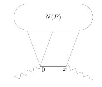
Figure 1:

Figure 2:

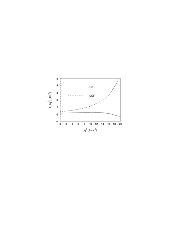
Figure 3:

Figure 4:

Figure 5:

Figure 6:

Figure 7:

References

• (1) I.I. Balitsky, V.M. Braun and A.V. Kolesnichenko, Nucl. Phys. B 312, 509( 1989); V.L. Chernyak and I.R. Zhitnitsky, $ibid.$ B 345, 137 (1990).
• (2) V. Braun, Light-Cone Sum Rules, hep-ph/9801222; V. Braun, Recent Development of QCD Sum Rules in Heavy Flavor Physics, hep-ph/9911206.
• (3) For a recent review on the QCD and light-cone QCD sum rule methods see: P. Colangelo and A. Khodjamirian, hep-ph/0010175, published in the Boris Ioffe Festschrift “At the Frontier of Particle Physics/Handbook of QCD”, 1495-1576, edited by M. Shifman (World Scientific, Singapore, 2001).
• (4) M. A. Shifman, A. I. Vainshtein and V. I. Zakharov, Nucl. Phys. B147, 385 (1979); B147, 448 (1979); V. A. Novikov, M. A. Shifman, A. I. Vainshtein and V. I. Zakharov, Fortschr. Phys. 32, 11 (1984).
• (5) G. P. Lepage and S. J. Brodsky, Phys. Rev. Lett. 43, 545(1979); 43, 1625(E) (1979); G. P. Lepage and S. J.  Brodsky, Phys. Rev. D. 22, 2157 (1980); V. L. Chernyak and A. R. Zhitnitsky, Phys. Rept. 112, 173 (1984).
• (6) V. M. Braun and I. E. Filyanov, Z. Phys. C 44, 157 (1989); P. Ball, V. M. Braun and H. G. Dosch, Phys. Rev. D 44, 3567 (1991); V. M. Belyaev, A. Khodjamirian and R. Rückl, Z. Phys. C 60, 349 (1993); V. Braun and I. Halperin, Phys. Lett. B 328, 457 (1994); V. M. Belyaev, V. M. Braun, A. Khodjamirian and R. Rückl, Phys. Rev. D 51, 6177 (1995); P. Ball and V. M. Braun, $ibid.$ D 58, 094016 (1998); A.  Khodjamirian, Nucl. Phys. B605, 558 (2001).
• (7) E. Bagan, P. Ball and V.M. Braun, Phys. Lett. B 417, 154 (1998); A. Khodjamirian, R. Ruckl and C.W. Winhart, Phys. Rev. D 58, 054013 (1998); A. Khodjamirian et al., $ibid.$ D 62, 114002 (2000); P. Ball, JHEP 9809, 005 (1998); P. Ball and R. Zwicky, $ibid.$ 0110, 019 (2001).
• (8) A. Ali, V. M. Braun, and H. Simma, Z. Phys. C 63, 437 (1994); P. Ball and V. M. Braun, Phys. Rev. D 55, 5561 (1997).
• (9) B. Grinstein, Nucl. Phys. B339, 253 (1990); E. Eichten and B. Hill, Phys. Lett. B 234, 511 (1990); A. F. Falk, H. Georgi, B. Grinstein, and M. B. Wise, Nucl. Phys. B343, 1 (1990).
• (10) M. Neubert, Phys. Rept. 245, 259 (1994).
• (11) Y. B. Dai and S. L. Zhu, Phys. Rev. D 58, 074009 (1998); S. L. Zhu and Y. B. Dai, Phys. Lett. B 429, 72 (1998); S. L. Zhu and Y. B. Dai, Phys. Rev. D 59, 114015 (1999); W. Y. Wang and Y. L. Wu, Phys. Lett. B 515, 57 (2001); J. G. Körner, C. Liu and C. T. Yan, Phys. Rev. D 66, 076007 (2002).
• (12) V. M. Braun, R. J. Fries, N. Mahnke, and E. Stein, Nucl. Phys. B589, 381 (2000); B607, 433(E)(2001).
• (13) C. S. Huang, C. F. Qiao and H. G. Yan, Phys. Lett. B 437, 403 (1998); R. S. Marques de Carvalho, F. S. Navarra, M. Nielsen, E. Ferreira and H. G. Dosch, Phys. Rev. D 60, 034009 (1999).
• (14) A. Datta, Semi-Leptonic Decays of $\Lambda_{c}$ and $\Lambda_{b}$ Baryons involving Heavy to Light Transitions and the determination of $V_{ub}$, hep-ph/9504429; M. A. Ivanov, V. E. Lyubovitskij, J. G. Korner and P. Kroll, Phys. Rev. D 56, 348 (1997);
• (15) W. Loinaz and R. Akhoury, Phys. Rev. D 53, 1416 (1996); H. H. Shih, S. C. Lee and H. n. Li, $ibid.$ D 59, 094014 (1999).
• (16) B. L. Ioffe, Nucl. Phys. B188, 317 (1981);E: B191, 591 (1981); Z. Phys. C 18, 67 (1983); V. M. Belyaev and B. Yu. Blok, Z. Phys. C 30, 151 (1983); M. A. Ivanov et al., Phys. Rev. D 61, 114010 (2000); D. W. Wang and M. Q. Huang, $ibid.$ D 67, 074025 (2003).
• (17) V. M. Braun, A. Lenz, N. Mahnke, and E. Stein, phys. Rev. D 65, 074011 (2002); A. Lenz, M. Wittmann and E. Stein, Phys. Lett. B 581, 199 (2004).
• (18) V. L. Chernyak and I. R. Zhitnitsky, Nucl. Phys. B246, 52 (1984); I. D. King and C. T. Sachrajda, $ibid.$ B279, 785 (1987); V. L. Chernyak, A. A. Ogloblin and I. R. Zhitnitsky, Sov. J. Nucl. Phys. 48, 536 (1988); Z. Phys. C 42, 583 (1989).
• (19) I. I. Balitsky and V. M. Braun, Nucl. Phys. B311, 541 (1989).
• (20) M. Diehl, T. Feldmann, R. Jakob, and P. Kroll, Eur. Phys. J. C 8, 409 (1999).
• (21) V. M. Braun, A. Khodjamiran, and M. Maul, Phys. Rev. D 61, 073004 (2000).
• (22) E. Bagan, P. Ball, V. M. Braun and H. G. Dosch, Phys. Lett. B 278, 457 (1992).
• (23) T. Mannel, W. Roberts, and Z. Ryzak, Nucl. Phys. B355, 38 (1991).
• (24) E. V. Shuryak, Nucl. Phys. B 198, 83 (1982); A. G. Grozin and O. I. Yakovlev, Phys. Lett. B 285, 254 (1992); Y. B. Dai, C. S. Huang, C. Liu and C. D. Lu, $ibid.$ B 371, 99 (1996); D. W. Wang, M. Q. Huang and C. Z. Li, Phys. Rev. D 65, 094036 (2002).
• (25) D. W. Wang and M. Q. Huang, Phys. Rev. D 68, 034019 (2003).
• (26) K. Hagiwara et al., Particle Data Group, Phys. Rev. D 66, 010001 (2002).