Skyrmion formation in 1+1 dimensions with chemical potential

Abstract

Formation of topological objects during phase transitions has been discussed extensively in literature. In all these discussions defects and anti-defects form with equal probabilities. In contrast, many physical situations, such as formation of baryons in relativistic heavy-ion collisions at present energies, flux tube formation in superconductors in the presence of external magnetic field, and formation of superfluid vortices in a rotating vessel, require a mechanism which can bias (say) defects over anti-defects. Such a bias can crucially affect defect-anti-defect correlations, apart from its effects on defect density. In this paper we initiate an investigation for the basic mechanism of biased formation of defects. For Skyrmions in 1+1 dimensions, we show that incorporation of a chemical potential term in the effective potential leads to a domain structure where order parameter is spatially varying. We show that this leads to biased formation of Skyrmions.

Key words: Topological defects, defect formation, chemical potential, Skyrmion

I Introduction

Production of topological defects is of considerable importance in the context of the early universe. Many particle physics models of unification of forces predict the existence of topological defects. These defects may be produced during various phase transitions in the early universe [1]. The first detailed theory of formation of topological defects, in the context of the early universe, was proposed by Kibble [2, 3]. However, the basic physical picture of the Kibble mechanism applies equally well to the large variety of topological defects known to arise in condensed matter systems [4, 5]. This allows the possibility of testing the Kibble mechanism in various condensed matter systems, see refs. [6, 7, 8, 9, 10]. In fact, the basic mechanism has many universal predictions which make it possible to use condensed matter experiments to carry out rigorous experimental tests of these predictions made for the defects in cosmology [9, 10]. The Kibble mechanism has also been used to study baryon formation during chiral symmetry breaking transition in relativistic heavy ion collisions [11, 12, 13] within the context of Skyrmion picture of baryons. There are important issues for the case of continuous transitions where the issue of relevant correlation length has been analyzed by Zurek [4]. In this Kibble-Zurek mechanism, defect formation is determined by the critical slowing down of the order parameter and depends on the rate of transition etc.

In all these discussions of formation of topological defects (here, for the sake of uniform terminology, we will use the term topological defect even for Skyrmions, though they are not defects in the usual sense) defects and anti-defects form with equal probabilities. However, there are many physical situations where formation of defects is favored over the anti-defects (or vice-versa). For example, in discussing the formation of flux tubes in type II superconductors in the presence of external magnetic field there will be a finite density of flux tubes, all oriented along the direction of external field (which we call as strings, the opposite orientation being associated with anti-strings). In addition there will be random formation of strings and anti-strings. Thus the basic mechanism of defect formation here should be able to account for the bias in the formation of strings over anti-strings. Formation of superfluid vortices (e.g. in ⁴He) with the superfluid transition being carried out in a rotating vessel will also produce biased vortex formation.

A similar situation arises in the context of Skyrmion picture of baryon formation. When one wants to study baryon formation during chiral phase transition in relativistic heavy-ion collisions, then one has to deal with the situation of non-zero baryon excess over antibaryons. This is certainly true for energies up to SPS. Even for RHIC, the baryon chemical potential is about 50 MeV for the central rapidity region [14]. This requires that the basic mechanism of Skyrmion formation should be able to incorporate an intrinsic bias in favor of Skyrmions over anti-Skyrmions (depending on the sign of the chemical potential). Such a bias can not only affect the estimates of net density of Skyrmions and anti-Skyrmions, it can have crucial effects on the predictions relating to Skyrmion-anti-Skyrmion correlations.

It is known that the topological models of formation of defects imply very specific defect-anti-defect correlations [10]. Predictions of these correlations, have a very important advantage over the predictions of defect density (as discussed in ref.[10]). In situations where there is no natural accurate determination of the correlation length, as in the case of heavy-ion collisions, reasonable predictions of defect (Skyrmion) density cannot be independently made. Essentially, given a value of correlation length, any baryon density can be fitted. In contrast, the predictions of defect-anti-defect correlations can be put in a universal form such that they only depend on average defect/anti-defect separation (i.e. defect/anti-defect density $\rho$) [10]. With experimentally observed value of $\rho$, theory of defect formation makes a unique prediction about defect-anti-defect correlations. This is well understood for the unbiased defect/anti-defect formation situation [10]. Such correlations need to be understood for the case of biased formation, where clearly a bias of (say) defects over anti-defects may affect these correlations in a crucial manner. Thus, once the theory of defect formation is extended for the situation of non-zero chemical potential, this can be used to make very specific predictions about baryon-anti-baryon correlations in heavy ion collisions. Another important point is that in QCD the baryon number is strictly conserved. This implies that in a given region undergoing chiral phase transition, net Skyrmion number produced must be constrained (to be equal to the net baryon number of that region).

In this paper we initiate a study for incorporating the effects of a bias in the theory of defect formation via the Kibble mechanism. We will first motivate the basic ideas using physical picture of flux tube formation in the presence of external field. We will see that this necessitates changing the basic picture of elementary domain where the order parameter is conventionally taken to be constant. In contrast, if the symmetry breaking phase transition (i.e. superconducting transition) occurs in the presence of external magnetic field then due to the presence of non-zero vector potential the order parameter should be taken to vary within a domain. We mention here that the prescription of order parameter inside a given domain, and even more importantly, the prescription for the inter-domain variation of order parameter (the so called geodesic rule) is ambiguous for the case of gauge theories [15]. However, even apart from those considerations, it will be clear (as discussed below) that biased formation of strings cannot occur unless one either modifies the geodesic rule, or introduces the spatial variation of the order parameter within a domain. (We mention here that we are assuming that the flux tube production is not dominated by fluctuations of magnetic field, e.g. as discussed in ref.[16]).

We will next analyze the case of Skyrmion formation. Here a bias in the formation of (say) Skyrmions is expected if there is non-zero chemical potential for baryon number. We will see that the introduction of a chemical potential term in the effective potential for the linear chiral sigma model will lead to spatial variation of order parameter being preferred, having lower free energy than the case of constant order parameter. This bias can be exactly calculated for the simpler case of 1+1 dimensions. Even though the nature of exact bias and its implications is complicated to analyze for higher dimensions, we expect similar techniques to work there. We hope to discuss that in a future work.

The paper is organized in the following manner. Section II discusses the basic idea of biasing defects for the case of flux tube formation in a superconductor in the presence of external magnetic field. In rest of the paper we discuss the case of Skyrmions in one space dimension. In section III we describe the modified picture of Skyrmion formation in the presence of a chemical potential term. In section IV we present the analytical estimate as well as numerical simulation results for the case when the physical space (taken for simplicity to be $S^{1}$, as discussed below) consists of only two domains. Numerical simulation results for the 3-domain case are presented in Sect.V. Sect. VI presents discussions and conclusions.

II Example of superconductor in external field

We first discuss the case of a type II superconductor in 2 space dimensions. This discussion will only be qualitative. Our purpose here is to bring out the naturalness of spatially varying order parameter within a domain in the presence of external magnetic field. Detailed discussion of spatial variation for this case will be deferred for a future work as this case has fundamental differences from the present case of Skyrmion. (For superconductors, bias originates from non-zero vector potential in the covariant derivative. Also 2+1 dim. case is much more difficult to analyze than the 1+1 dim. case which we discuss in the present paper).

The free energy density for the superconductor is given by,

$$F=|D_{i}\psi|^{2}+a(T)|\psi|^{2}+b|\psi|^{4}$$ (1)

$$D_{i}\psi=(\partial_{i}-ieA_{i})\psi~{};~{}i=1,2.$$ (2)

$A_{i}$ are the spatial components of the vector potential and $b>0$, while $a(T)>0$ for $T>T_{c}$ and $a(T)<0$ for $T<T_{c}$. $T_{c}$ is the critical temperature. Here, we are not including the field strength term. We are only focusing on the nature of order parameter within a domain in the superconducting phase from the point of view of the Kibble mechanism. Thus full dynamics of gauge field is not being considered here. (As mentioned above, we are also not considering here the situation when flux tube formation may arise due to fluctuations of the magnetic field [16]).

For $T<T_{c}$, in the superconducting state, $D_{i}\psi=0$ inside a superconductor which leads to flux quantization. In the absence of any external fields, the formation of flux tubes during a superconducting transition can be studied using the Kibble-Zurek mechanism. The physical 2 dimensional region undergoing the phase transition will develop a domain structure. Phase $\theta$ of $\psi$ will be constant within a domain. $\theta$ varies randomly from one domain to another while $\theta$ interpolates smoothly in between two adjacent domains (see ref.[15] for a discussion of this point). Using this the probability of flux vortices (for two space dimensions) can be determined to be 1/4 per domain [17].

Now consider the case when the phase transition is happening in the presence of external magnetic field. This will require that there be a net excess of strings over anti-strings. (Note that even with the conventional mechanism, net string number is not zero in a given sample. However, there the net string number could be positive or negative, with zero average.) One way to implement an overall excess of strings over anti-antistrings can be to impose the net winding number at the boundary of the sample. This way one can unambiguously fix the net excess of flux vortices over anti-vortices. However, if one simply fixes the variation of $\theta$ at the boundary of the sample, and keeps the conventional picture of defect formation for the inside region (i.e. random $\theta$ for each domain and geodesic rule for regions in-between the domains), then it is easy to see that essentially all the excess vortices will be concentrated within one domain thickness of the boundary. This is because for regions which are more than one domain distance away from the boundary, conventional defect formation applies. This leads to defect-anti-defect symmetry on statistical basis for those regions. Even if there is slight excess of vortices in the interior region in one case, anti-vortices may be in excess in the next case (with this excess being proportional to $N^{1/4}$, $N$ being net number of defects+anti-defects in the interior region). Thus, essentially entire excess vortex number imposed by the boundary winding will have to be carried by the one domain thick shell within the boundary.

Similar situation can be argued even for the case of Skyrmions. It is important to realize that net winding for integer winding Skyrmions cannot be fixed in this manner by prescribing a winding at the boundary. This is because each full integer winding Skyrmion represents a compactified region of space where the boundary of a ball (disk in 2 space dimensions and 3-ball in 3 space dimensions) has a constant value of the chiral field. Thus there is no memory of winding of Skyrmion at the boundary of the region. However, as discussed in the literature [12], integer winding Skyrmions almost never form during a phase transition. It is only the partial winding Skyrmions which have reasonable probability of formation. The winding numbers of these partial winding Skyrmions can be fixed by prescribing the winding at the boundary. For example, for 2-d Skyrmions with Skyrmion winding being carried by the polar angle $\theta$ and the azimuthal angle $\phi$ on $S^{2}$, one can assume that $\theta$ never approaches $\pi$ outside the partial Skyrmions (with $\theta=0$ at the center of the Skyrmion). Then $\phi$ windings will determine whether one has Skyrmion or anti-Skyrmion. Fixing $\phi$ winding at the boundary of the 2-dimensional region will fix the net Skyrmion number, assuming that these partial Skyrmions will evolve to become integer Skyrmions. (Actual situation is more complicated as the variation of the polar angle $\theta$ may in general be different in different partial Skyrmion regions.) It may thus be possible that one will end up with the same situation as discussed above for the case of superconductor. That is, if a net Skyrmion winding is fixed at the boundary of the region, then the excess Skyrmions will all be essentially concentrated within few domains thick shell at the boundary.

Clearly this situation is not satisfactory. When excess flux vortices form due to external field, they are roughly uniformly distributed in the sample. Similarly, non-zero baryonic chemical potential will lead to a uniform excess in the baryon density over anti-baryon density. It is then clear that one needs to modify the whole picture of defect formation itself. As we will discuss below, fixing boundary windings can be used to implement exact conservation of defect number, say Skyrmion number. (This exact conservation may not be needed for the superconductor case where a net statistical excess of strings may be sufficient.) However, this has to be supplemented with modification in the basic defect formation picture in order to distribute the excess defects uniformly in the whole region. We now discuss this modification of the defect formation picture.

Let us again consider the case of a 2-dimensional region undergoing superconducting transition in the presence of external field. Until the order parameter field $\psi$ settles to its thermodynamic equilibrium value, there will be non-zero currents present and $D_{i}\psi$ will not necessarily vanish inside the superconductor. As $\psi$ approaches the equilibrium value, the magnetic field will be pushed out of the superconducting regions, getting trapped in the form of isolated vortices, and $D_{i}\psi$ will approach zero inside the superconducting region. If $\theta$ is taken to be constant inside each domain, as in the case of zero external field, then $A_{i}$ will also be constant inside each domain. This will require modification for the standard geodesic rule to account for extra vortices due to external field. Though this possibility cannot be easily ruled out (and needs to be examined carefully), it is certainly not very natural. This leads to the requirement that the biased formation of vortices over anti-vortices is entirely due to regions in-between the domains. Certainly, for a second order transition, the splitting of the region in terms of elementary domains and inter-domain regions is somewhat ambiguous. Domains do not have completely constant $\theta$ with all the $\theta$ variation remaining in the inter-domain regions. In fact, one can very well consider the inter-domain regions as elementary domains with original domains becoming the inter-domain regions. Statistically it should not make much difference in calculation of defect formation probabilities. Thus, if vortices are to be biased over anti-vortices, then it looks unnatural to assume that the domain picture remains unchanged while only the inter-domain regions implement the biased vortex formation.

A more satisfactory picture, which as we will see below, also naturally fits with the picture of Skyrmion formation with non-zero chemical potential, is the following. As there is a net magnetic field going through the region, we assume that $\theta$ inside each domain has spatial variation. With $D_{i}\psi=0$ inside each domain, it will imply specific biased variation of the vector potential inside each domain. Combined with a suitably modified geodesic rule, this will lead to an overall excess of flux vortices over anti-vortices. (Similarly, if we consider superfluid vortices forming during phase transition in a rotating vessel, then due to already present fluid velocity, a non-zero gradient of the condensate phase should naturally arise.) For the superconductor case, the exact nature of the spatial variation of $\theta$ (and consequently of $A_{i}$) will depend on the choice of gauge etc.

There are several points here that one should be careful about. First, as mentioned above, the dynamics of flux tube formation may be dominated by fluctuations of magnetic field, as discussed in ref.[16]. The considerations discussed here do not apply to such cases. Second point is that the uniform field at the beginning of phase transition will become unstable at the end of the transition, after all that is how the flux tubes form. The choice of vector potential to bias $\theta$ variation should take into account such a dynamics of the magnetic field. These are complex issues and need to be examined in detail. These issues for the case of 2-dimensional superconductor, and for superfluids, will be discussed in a future work. The arguments we have discussed for this case are very crude. Our purpose here was only to physically motivate that spatially varying order parameter within a domain can arise in a physical example. As we will see below, same effect can arise by postulating a chemical potential term for the free energy for the Skyrmion case.

III Skyrmions in 1+1 dimensions

Above, we have tried to argue qualitatively what kind of modifications are needed for the basic domain picture to implement the biased formation of defects. We now consider the case of Skyrmion formation in one space dimension where these ideas can be concretely implemented. To represent the situation of a nonzero chemical potential, we will add a $-\mu N$ term to the effective potential of linear chiral sigma model (see ref.[18] in this context). Here $N$ is the topological Skyrmion winding number to be identified with the baryon number (in 3+1 dimensions). In one space dimension we can write the appropriate free energy (for possibly inhomogeneous field configurations) as follows. For simplicity of presentation we use dimensionless variables. We divide the free energy density by $m^{2}$, the coefficient of $\phi^{2}$ term. Length scales are measured in units of $m^{-1}$, and the chemical potential $\mu$ in units of $m$. We can now write down the dimensionless free energy as,

$$F=\int[|\partial_{x}\phi|^{2}-|\phi|^{2}+\lambda|\phi|^{4}-\mu n(x)]dx,$$ (3)

$$n(x)={1\over 2\pi}\partial_{x}\theta.$$ (4)

Here $N=\int n(x)dx$ is the Skyrmion number. $\phi$ takes values on a circle $S^{1}$, which can be written as $\phi=\phi_{0}e^{i\theta}$.(We mention that there is no strictly conserved topological current for the case of linear sigma model, hence no exact conservation of Skyrmion number. This is why, to implement exact conservation of baryons we will need to fix the winding number at the boundary of the sample.)

Let us determine what configuration of $\phi$ is preferred for the domain. In one space dimension only topological configurations are the Skyrmions. For these, the magnitude of $\phi$ can be taken to be constant $\phi_{0}$ for the entire 1 dimensional physical space. The quadratic and quartic terms in $\phi$ in Eq.(3) then add up to give a constant which we can neglect in the following discussion. The relevant terms in $F$ from Eq.(3) are,

$$F_{d}=\int[\phi_{0}^{2}(\partial_{x}\theta)^{2}-{\mu\over 2\pi}\partial_{x}\theta]dx.$$ (5)

Note that, Skyrmion number $N$ is a topological invariant only when boundary conditions are fixed. Further, we determine the local value of equilibrium order parameter by minimizing the free energy density hence $n(x)$ can affect the determination of the equilibrium value of the order parameter as we show below. The chemical potential term, being a total derivative, does not contribute to the field equation $\partial_{x}^{2}\theta=0$. A general solution of this equation is $\theta(x)=\alpha x+\theta_{0}$. As the free energy density in the expression for $F_{d}$ depends only on $\partial_{x}\theta=\alpha$, we minimize it with respect to $\alpha$ to get,

$$\alpha=\partial_{x}\theta={\mu\over 4\pi\phi_{0}^{2}}~{}\equiv~{}\mu^{\prime}.$$ (6)

We therefore see that for non-zero $\mu$, constant $\theta$ is not preferred as an equilibrium configuration. This is an unconventional result. Normally, for a theory where some internal symmetry is spontaneously broken, the vacuum is translationally invariant. This is how the effective potential is calculated, starting from the effective action, and restricting to constant field configuration. Spatial variations of the order parameter are conventionally discussed only as departure from the equilibrium situation. The non-trivial part of the above equation is that spatial variation of the order parameter is present even for the equilibrium configuration of the order parameter. This is happening due to the fact that the chemical potential term for the Skyrmion number is expressed in terms of the derivative of the order parameter field $\phi$. As long as derivative terms come with positive definite contributions to the free energy, the equilibrium order parameter configuration (i.e. with lowest free energy) will be spatially constant. This is what happens with the conventional $(\partial_{i}\phi)^{2}$ term. Even the presence of Skyrme term [19] will lead to the same conclusion, i.e. constant order parameter. The situation is completely different with the above chemical potential term. This term is linear in the derivative of $\phi$ and hence not positive definite. Therefore, it is no longer certain that the equilibrium configuration will be that of a constant $\phi$. It will be interesting to investigate how one can justify this type of picture at a more fundamental level. For example, for QCD with fundamental degrees of freedom being quarks and gluons, a chemical potential term for the baryon number apparently has no reason to lead to a situation where the equilibrium order parameter should have spatial variations. However, as we have argued above, in the chiral models, the chemical potential term for the baryon (Skyrmion) number should naturally lead to spatial variation for the equilibrium order parameter. In this context, we mention ref.[18] where a chemical potential term for the Skyrmion number has been derived.

With Eq.(6), our strategy for determining the formation of Skyrmion will be as follows. We split the physical space, say x axis, in terms of elementary domains which are one dimensional segments for the present case. We choose random values of $\theta$ in the middle of each domain. In a given domain, the spatial variation of $\theta$ from one end to the other end is then determined by integrating Eq.(6). With uniform variation of $\theta$ across the domain, net $\theta$ variation within a given domain of size equal to correlation length $\xi$, will be,

$$\Delta\theta={\mu\xi\over 4\pi\phi_{0}^{2}}~{}=~{}\mu^{\prime}\xi.$$ (7)

We still need to specify how $\theta$ is supposed to interpolate in between two adjacent domains. Conventionally (i.e. with $\mu=0$) one simply uses the geodesic rule which is the statement of minimizing the free energy in the inter-domain region. Note that this geodesic rule does not require specification of how large the inter-domain region actually is. With non-zero $\mu$, one needs to specify more details about the inter-domain region. We will still follow the spirit of the geodesic rule, i.e. minimize the net free energy in the inter-domain region. However, due to the chemical potential term it does not lead to the conventional geodesic rule. Depending on the value $\theta$ at the end of one domain, and the value $\theta^{\prime}$ at the beginning of the next domain, it may happen that the longer path on the vacuum manifold $S^{1}$ may be preferred in some cases. An example of this is shown in Fig.1 where, due to the chemical potential term, the anti-clockwise variation from $\theta$ to $\theta^{\prime}$ may have lower free energy compared to the shorter clock-wise variation. We compare the values of $F_{d}$ (Eq.(5)) for the two paths on $S^{1}$, with opposite orientations, joining $\theta$ and $\theta^{\prime}$. The path with lower value of $F_{d}$ is selected to represent the $\theta$ variation in the inter-domain region. We take uniform variation of $\theta$ for both paths, any other variation should give higher free energy for a given orientation of path (unless the chemical potential term in Eq.(5) becomes completely dominant). The choice of the path not only depends on $\theta$ and $\theta^{\prime}$, but also on the domain size $\xi$ as well as the size of the inter-domain region (and obviously on $\Delta\theta$ in Eq.(7)). We therefore introduce another length scale $\chi$ which represents the size of the inter-domain region. We will present results for varying values of $\xi$ and $\chi$. These two different length scales have a clear meaning in a first order transition via bubble nucleation. The core of bubble representing uniform magnitude of the order parameter will have size $\xi$ while the bubble wall region for two coalescing bubbles can represent the inter-domain region with size $\chi$. (Just like the conventional case of $\mu=0$, free energy in the inter-domain region will be higher which, for the bubble case, can come from the energy of coalescing bubble walls). For a second order transition, definition of domain and inter-domain regions is much more fluid. One can take $\xi$ to represent the region where the order parameter variation is given by the field equation (Eq.(7)) whereas, in the inter-domain region larger variations of $\theta$ may occur.

Using Eqs.(5) and (7), it is easy to show that, for $0<\theta<\theta^{\prime}<2\pi$, the anti-clockwise variation from $\theta$ to $\theta^{\prime}$ has lower free energy compared to the clockwise variation if the following condition is satisfied,

$$\theta^{\prime}-\theta<\Delta\theta{\chi\over\xi}+\pi.$$ (8)

Here $\theta$ and $\theta^{\prime}$ are the values of the phase at the two end points of a given inter-domain region (i.e., say, $\theta$ at the end of one domain and $\theta^{\prime}$ at the beginning of the next domain). From Eq.(8) we see directly that for $\Delta\theta>0$, anti-clockwise variation may be preferred even when this variation is larger than $\pi$.

Due to this detailed rule for determination of $\theta$ in the inter-domain region, the final probability becomes dependent on the length scales $\xi$ and $\chi$ in a complicated manner. It then becomes very difficult to determine analytically the probability of Skyrmion formation in this case. In the following, we will present an analytical calculation of the probability for the two domain case, but for three domain case we will need to resort to numerical simulation for determination of this probability.

Another important point is that the formation of Skyrmion is actually very different from the formation of other topological defects like monopoles, strings etc. This is because Skyrmions require constant boundary conditions for their topological description. These issues have been discussed in the literature. One determines the probability of formation of partial winding Skyrmion which is expected to subsequently evolve into a full integer winding Skyrmion [12]. However, these complications are not relevant for the main point of the present work which is to investigate the effects of non-zero chemical potential on the basic theory of defect formation.

To avoid the issues of boundary conditions etc. for Skyrmion case, we will further simplify the problem. For the present case of one space dimension, we consider the physical space to be compact, i.e. a circle $S^{1}$. Further we consider the size of the circle to be sufficiently small so that it can accommodate only a couple of correlation domains which are sufficient to form one Skyrmion in the whole circle. This way the issue of boundary condition becomes irrelevant. For $\mu=0$ case this would have been the same as the calculation of the probability of winding around a loop going through couple of domains, i.e. the probability of vortices.

IV two domain case

We know that for $\mu=0$ case there is no possibility of any winding unless one considers three or more domains. This is not the case for $\mu\neq 0$ case. Due to the spread of $\theta$ (given by Eq.(7)) within a given domain, it is easy to see that even if the physical space $S^{1}$ has only two domains, one can still get non-trivial windings. Each domain already contains partial positive windings (for $\mu>0$). Inter-domain regions only need to complete this winding. It is also easy to convince oneself that there is no possibility of getting any anti-winding with only two domains (again, for $\mu>0$ case). [Positive windings correspond to the case when, as one goes around the closed path in physical space in an anti-clockwise/clockwise direction, then the variation of $\theta$ in the order parameter space $S^{1}$ is also in an anti-clockwise/clockwise direction. Negative windings will correspond to the case when the direction of variation of $\theta$ in the order parameter space is opposite to the direction of the path in the physical space.]

Consider the physical space $S^{1}$ (as discussed above) consisting of two domains as shown in Fig.2. The two random values of $\theta$ at the centers of the two domains are $\alpha$ and $\beta$. The anti-clockwise variation of $\theta$ as given by Eq.(7) within each domain is shown in the figure. Arrows in the figure show anti-clockwise path taken in the physical space to calculate the winding of $\theta$. For notational simplicity, we denote the beginning values of $\theta$ (along the anti-clockwise path in the physical space) in each of the two domains as follows,

$$\alpha-{\Delta\theta\over 2}\rightarrow\theta_{1},\\ {\rm\quad and\quad}\beta-{\Delta\theta\over 2}\rightarrow\theta_{2}.\\$$ (9)

With this, the values of $\theta$ at the other ends of each domain become $\theta_{1}+\Delta\theta$ and $\theta_{2}+\Delta\theta$ respectively. In Fig.2, domains (of size $\xi$) are shown by the dashed curves and inter-domain regions (of size $\chi$) are shown by the dotted curves.

We will set $\theta_{1}=0$, so that all other angles shown in Fig.2 are less than 2$\pi$ and are measured from $\theta_{1}=0$. We also assume that $\Delta\theta$ as given in Eq.(7) is less than $\pi$ to simplify the analytical estimates. Within each of the two domains the variation of $\theta$ is equal to $\Delta\theta$ (as given in Eq.(7)) and is in the anti-clockwise direction on the vacuum manifold $S^{1}$. The formation of defect or antidefect then depends on whether in the two inter-domain regions $\theta$ interpolates in the clockwise direction or in the anti-clockwise direction. (We again repeat that we are using the terms defect and antidefects even for Skyrmions and anti-Skyrmions, though they are not defects in the usual sense). Let us call the inter-domain region from $\theta_{1}+\Delta\theta\rightarrow\theta_{2}$ as Junction 1 and the inter-domain region from $\theta_{2}+\Delta\theta\rightarrow\theta_{1}$ as Junction 2. Then there will be four cases depending on the direction of the variation of $\theta$ at these two junctions.

(1): Junction 1 clockwise, Junction 2 anti-clockwise

(2): Junction 1 anti-clockwise, Junction 2 clockwise

(3): Junction 1 clockwise, Junction 2 clockwise

(4): Junction 1 anti-clockwise, Junction 2 anti-clockwise

As $\theta_{1}$ has been set equal to zero, the value of $\theta_{2}$ will decide which of the above cases is preferred as the lowest free energy configuration, and hence the resulting winding number.

First consider the situation when, on the vacuum manifold $S^{1}$, $\theta_{2}$ lies in between $\theta_{1}(=0)$ and $\theta_{1}+\Delta\theta(=\Delta\theta)$. It is easy to see that in this situation, cases (1) and (2) give rise to one positive winding each, case (3) gives no winding and case (4) leads to a positive winding number 2 defect.

Using Eq.(8), we see that for case (4) the requirement of anti-clockwise variation at Junction 1 implies

$$2\pi-\Delta\theta+\theta_{2}<\Delta\theta\frac{\chi}{\xi}+\pi\quad\Rightarrow\quad\theta_{2}<\Delta\theta(\frac{\chi}{\xi}+1)-\pi.$$ (10)

If we assume that the values of chemical potential, the domain size $\xi$, and the inter-domain size $\chi$ are such that,

$$\Delta\theta<{\pi\over(\frac{\chi}{\xi}+1)},$$ (11)

then we see that the requirement at junction 1 cannot be satisfied since $\theta_{2}>0$. Thus no winding 2 defects will form in this case. We will assume this to be the case for the analytical estimates. Thus, here, we are calculating the probability of defects when the bias given by the chemical potential (Eq.(7)) is not very large. We do this for the sake of simplicity as analytical estimates for large $\Delta\theta$ become more complicated (with larger variety of configurations contributing to defect formation). When we present numerical results, then we will present results for larger values of $\Delta\theta$ also.

For case (2) we see that the requirement on Junction 1 is the same as in case (4). With the requirement on $\Delta\theta$ as given in Eq.(11), we thus see that no defects will form for the case (2).

Now let us discuss case (1). The conditions on $\theta_{2}$ from Junction 2 and Junction 1 are, respectively,

$$\theta_{2}>-\Delta\theta(\frac{\chi}{\xi}+1)+\pi\equiv A$$ (12)

$$\theta_{2}>\Delta\theta(\frac{\chi}{\xi}+1)-\pi=-A.$$ (13)

Note that with Eq.(11), $A>0$. Also, we are discussing the case when $0<\theta_{2}<\Delta\theta$ hence the allowed range for $\theta_{2}$ (from Eq.(12)) is $\Delta\theta-A=\Delta\theta(\frac{\chi}{\xi}+2)-\pi$. Thus, if we make a stronger restriction (compared to that given by Eq.(11)) on $\Delta\theta$ such that,

$$\Delta\theta<{\pi\over(\frac{\chi}{\xi}+2)},$$ (14)

then no defects will form in case (1) also. We will assume that Eq.(14) is satisfied by the parameters so that no defects are formed when $\theta_{2}$ lies between $0(=\theta_{1})$ and $\Delta\theta$.

Let us now consider the situation when $\theta_{2}>2\pi-\Delta\theta$. (Note, $\theta_{2}<2\pi$.) Again completing path anticlockwise in the physical space in Fig.2, one can see that in this situation also, cases (1) and (2) give rise to one positive winding (assumed to be anti-clockwise winding) each, case (3) gives no winding and case (4) leads to a winding number 2 defect. Following the arguments as above for all the four junction conditions, one can show that, with Eq.(14), no defects are formed in this case.

Finally we discuss the situation when $\theta_{2}$ takes any value in the rest of the vacuum manifold, i.e. $\Delta\theta<\theta_{2}<2\pi-\Delta\theta$. In this situation one can see that cases (1) and (2) do not give any defects. Case (3) gives an anti-defect whereas case (4) gives formation of winding one defect. As we have mentioned earlier, for the two domain case no anti-winding defects can form. One can see it here directly also by requiring the conditions on Junction 2 and Junction 1 for case (3), i.e.

$$2\pi-\theta_{2}-\Delta\theta>\Delta\theta\frac{\chi}{\xi}+\pi$$ (15)

$$\theta_{2}-\Delta\theta>\Delta\theta\frac{\chi}{\xi}+\pi,$$ (16)

respectively. These give,

$$\theta_{2}<-\Delta\theta(\frac{\chi}{\xi}+1)+\pi$$ (17)

$$\theta_{2}>\Delta\theta(\frac{\chi}{\xi}+1)+\pi.$$ (18)

These conditions are mutually inconsistent since $\Delta\theta(\frac{\chi}{\xi}+1)>0$. Thus no antidefects form.

We thus consider the last case (4). Junction 2 condition gives

$$\theta_{2}>-\Delta\theta(\frac{\chi}{\xi}+1)+\pi.$$ (19)

Junction 1 condition gives,

$$\theta_{2}<\Delta\theta(\frac{\chi}{\xi}+1)+\pi.$$ (20)

One can easily check that these conditions are consistent with the range of $\theta_{2}$ for this case, i.e. $\Delta\theta<\theta_{2}<2\pi-\Delta\theta$.

Thus, the allowed range of $\theta_{2}$ for the formation of winding one defects is

$$\theta_{2}^{\rm Range}=(2\Delta\theta)(\frac{\chi}{\xi}+1).$$ (21)

As $\theta_{2}$ can take any value between $0$ and $2\pi$, we conclude that the probability for the formation of winding one defects for the two domain case is

$$P=\frac{(\Delta\theta)(\frac{\chi}{\xi}+1)}{\pi}.$$ (22)

This expression is valid for the values of parameters such that Eq.(14) is satisfied. No antiwinding defects are formed for the two domain case.

We have carried out numerical simulation for the two domain case by randomly assigning values of $\theta_{1}$ and $\theta_{2}$ (note, that this is completely equivalent to assigning random values of $\theta$ at the middle of the domains) as shown in Fig.2. For each of the two junctions, we then compare the free energies (Eq.(5)) for the clockwise and the anti-clockwise variations of $\theta$ around the vacuum manifold and select the path with lower free energy. Net winding is then calculated for the anti-clockwise path in the physical space starting from, and ending at $\theta_{1}$. Fig.3 shows the results of numerical simulation. Symbols give the numerical simulation values of the probability $P$ which is the probability of positive windings as a function of $\Delta\theta$. (Here, as $\Delta\theta$ is varied, $\xi$ is kept fixed in Eq.(7).) Solid continuous lines show the plots of the analytical results in Eq.(22). This is plotted only up to the value of $\Delta\theta=\frac{\pi}{(\frac{\chi}{\xi}+2)}$ as allowed by Eq.(14). We see that simulation results completely agree with the analytical results. We had carried out simulation for 100,000 events so the numerical errors are negligible. One point here is that, although Eq.(22) seems to imply that only the ratio $\chi/\xi$ is relevant for the probability calculation, it is because we have restricted to small $\Delta\theta$ case. For larger values of chemical potential, the probability depends more generally on $\xi$ and $\chi$, though it becomes complicated to work out all possible configurations. We also note that for $\xi=1,\chi=2$, probability of 2-winding Skyrmions also becomes non-zero beyond $\Delta\theta\simeq 1.1$. For values of $\Delta\theta$ larger than this, the total probability plot for this case also includes the contributions from these 2-winding Skyrmions. (We do not plot the probabilities beyond $\Delta\theta\simeq\pi/2$ as for higher values even higher winding Skyrmions start forming and correspondence with the analytical estimates becomes more remote.) Double winding Skyrmions are counted as 2 times single winding Skyrmion. In this sense the total probability for this case represents the average number of positive winding Skyrmions.

V three domain case

For three domain case we do not attempt analytical estimate as it becomes very complicated. Physical space is divided in three domains (with three inter-domain regions) in a similar manner as the two domain case in Fig.2. Random values of the three angles in the three domains are chosen (at the beginning of each domain, which, as discussed for the two domain case, is equivalent to selecting random values at the middle of each domain). The path on the vacuum manifold is numerically determined for each inter-domain region by calculating free energies as before.

Figs.4 and 5 show plots for the case of three domains. Fig.4a shows the plots of the total probability $p_{+}$ of Skyrmion formation (giving average positive winding Skyrmion). We see that this increases with increasing value of $\Delta\theta$ (and hence $\mu$). Total probability is calculated by multiplying the number of Skyrmions of a given winding number by the winding number. The value of this probability $p_{+}$ thus refers to average positive winding Skyrmion number. Fig.4b shows the probability $p_{-}$ of anti-Skyrmion formation. AntiSkyrmions are found only with winding minus one for this three domain case. In Fig.4, we can make comparison with the conventional case of $\mu=0$. We thus see that plots of winding plus one and minus one intersect the y axis ($\mu=0$) at $p_{+}\simeq p_{-}\simeq 0.125$ (corresponding to the net probability = 1/4 of defect or anti-defect formation). We see that non-zero $\mu$ affects the probabilities very strongly. Interesting thing to note is that the net probability of formation of Skyrmion or anti-Skyrmion also increases with $\Delta\theta$, as shown in Fig.4c.

Fig.5a-d show plots of probabilities (again, average Skyrmion number) for positive winding Skyrmions for windings +1, +2, +3, and +4 respectively. (Note that for the dotted curve in Fig.5a, the probability of winding one Skyrmion becomes almost zero beyond $\Delta\theta\simeq 1.5$, which is responsible for the change of slope for the corresponding plot in Fig.4a.) We plot probabilities for values of $\Delta\theta<\pi$ (for Fig.4 and 5, except Fig.4b where plot is given only upto $\Delta\theta$ = 0.75 as $P_{-}$ becomes zero beyond this value). This is because of two reasons. First it already illustrates the basic features of probabilities of defect and antidefect formation in the presence of a bias. Secondly, already in this case very complex Skyrmion configurations (with winding numbers 3 and 4) start forming. The plots of total probability are then calculated by multiplying the number of Skyrmions of a given winding number by the winding number. The value of the probability thus refers to average Skyrmion number. For values of $\Delta\theta$ larger than $\pi$ even larger winding Skyrmions (winding 5) start forming and it becomes difficult to extract any pattern from the plots. In this sense the parts of the plots for smaller values of $\Delta\theta$ ($<\pi/2$) are most physical as they primarily contain Skyrmions up to winding 2, and one can get a feeling for how probabilities are changing with changing $\Delta\theta$.

Another point is that the probabilities depend in a complex manner on the two length scales $\xi$ and $\chi$. Though one may expect that $\theta$ variation within a domain, and its bias in the inter-domain region both should have similar effects. But our plots do not imply that. In fact, there is an important difference between the region of the domain and the inter-domain region in our model. Inside a domain, variation of $\theta$ is fixed by Eq.(6). Whereas in the inter-domain region the variation is fixed by the boundary conditions at the ends of the region and crucially depends on the length scales $\xi$ and $\chi$. It may be interesting to investigate this issue further, possibly by developing some scheme which treats the domain and inter-domain regions on a somewhat equal footing.

We have thus achieved our goal, that is, we have developed a mechanism which uniformly biases the formation of windings of one sign over the opposite windings. It is very satisfying that a very natural extension of the sigma model effective potential with a chemical potential term leads to qualitatively similar picture of spatially varying $\theta$ within an elementary domain as one expected in the case of flux tube formation for superconducting transition in the presence of external field (or the superfluid case).

VI Conclusions and Discussions

We mention an interesting possibility which arises from the observation in Fig.4 that anti-Skyrmion probability $p_{-}$ drops to zero at some value of $\Delta\theta$ (corresponding to some specific value of $\mu^{\prime}$) before the Skyrmion probability (average Skyrmion number) $p_{+}$ crosses the value 1. If one can get a similar plot for the realistic 3+1 dimensional case, then the value of chemical potential $\mu_{-}$, beyond which $p_{-}$ drops to zero, may have some relationship with the critical value of the chemical potential $\mu_{c}$ in the QCD phase diagram at T = 0 (for massless flavors, as explicit symmetry breaking has not been accounted for in the present model). This is because, for $\mu>\mu_{-}$ in our model, the effects of phase transition induced domain-to-domain fluctuations, (thermal or quantum), become sub-dominant compared to the effects of the bias generated by $\mu$, thereby leading to zero anti-baryon production. Any further increase in $\mu$ only creates more baryons, consistent with increasing $\mu$, without creating any anti-baryons. It seems reasonable to expect that for $\mu<\mu_{c}$ in the QCD phase diagram, the chiral transition (by varying temperature) should be able to produce at least some anti-baryons also, especially due to non-equilibrium nature of the domain structure of the chiral order parameter. For $\mu>\mu_{c}$ there is no phase transition, and for $T=0$ one does not expect any anti-baryons to be present. Similar thing is happening here where no anti-baryons are produced in our model for $\mu>\mu_{-}$, suggesting a possible relationship of $\mu_{-}$ with $\mu_{c}$. One could also explore whether $\mu_{c}$ could be related to the value of $\mu$ in our model beyond which the Skyrmion probability (average Skyrmion number) crosses 1. However, in that regime every domain will have a Skyrmion on the average and the situation will resemble less like the situation of a phase transition.

We note here that a term, similar to the chemical potential term in Eq.(3), has been used previously in the context of certain models of electroweak baryogenesis where, to favor baryons over anti-baryons, a CP violating term is introduced by writing an effective chemical potential term for the Chern-Simons number [20]. However, there this term corresponds to the winding number of the gauge fields, and not the Higgs field as in the present case. Hence, the chemical potential term in ref. [20] does not affect the vacuum configuration. It affects the evolution of the fields, thereby biasing the dynamics in favor of positive change in the Chern-Simon number. If a term like we use in the present paper can be written down for the Higgs field also in those models [20], then our results of the present paper suggest that one may be able to produce baryon asymmetry using biased production of texture configurations over anti-texture configurations (apart from any bias coming from dynamics). At the same time, discussions of the CP violating term in ref.[20] suggest that one may be able to bias production of Skyrmions over anti-Skyrmions by biasing the field evolution dynamics in favor of Skyrmions over anti-Skyrmions. Though here it would happen in different way compared to the case in ref.[20] where competing time scales of the Higgs field evolution and gauge field evolution play a crucial role. In the context of chiral models, one will utilize the fact that, as mentioned above, initially only partial winding Skyrmions are expected to form which evolve to full winding Skyrmions subsequently. If the dynamics could be favored for positive windings compared to negative windings then one can imagine that a large number of initial partial positive winding configurations will have chance of evolving to (positive) integer winding, while a lesser number of configurations will be able to evolve to (negative) integer windings. It will be interesting to investigate these possibilities.

Many steps remain to complete the program initiated in the present work. First, one needs to investigate the formation of Skyrmions in a one-dimensional space of large extent where issues of boundary conditions will play a role. Though, non-trivial aspects of evolution of partial winding Skyrmions into full winding Skyrmions are expected to occur only in 2 or higher 3 space dimensions. For 2 and 3 dimensions one needs to work out the exact nature of spatial variation of the chiral order parameter within a domain as well as for inter-domain regions. Then the above described program will be easily extended for these dimensions as well. Also, in the context of chiral phase transition in QCD, one would like to implement exact Skyrmion (baryon) number conservation. That is, for a given volume of physical space, defect formation mechanism should be able to produce a given amount of net Skyrmion excess over anti-Skyrmion. This is to represent the experimental situation where a given volume of quark-gluon plasma (QGP) in chirally symmetric state undergoes chiral symmetry breaking. Resulting net baryon number should exactly equal the baryon number contained in the original QGP region. (Neglecting any baryon diffusion across the boundary of the region under consideration.) As mentioned above, we can now achieve it in the following manner. We fix the winding at the boundary of the whole region to exactly equal to the required baryon number inside the boundary (i.e. the initial baryon number of the QGP volume). The problem of concentration of excess baryons near the shell (as mentioned above) can now be avoided by using the modified defect formation method for the interior region. The value of $\mu$ can be adjusted suitably such that it leads to uniform excess of baryon density from the shell to the interior region.

In conclusion, we have proposed a method to handle production of topological defects when physical situation requires excess of windings of one sign over the opposite ones. We have considered the case of Skyrmions in 1+1 dimensions and have shown that addition of a chemical potential term leads to modification in the order parameter distribution inside elementary domains leading to excess production of Skyrmions over anti-Skyrmions (for $\mu>0$, for negative $\mu$ anti-Skyrmions are preferred over Skyrmions). Extension of these techniques to the 3 dimensional case will give us a realistic Skyrmion formation mechanism which can be applied for the case of relativistic heavy-ion collisions. Same ideas will also help to investigate formation of flux vortices in superconductors in the presence of external magnetic field, as well as formation of superfluid vortices when the transition is carried out in a rotating vessel. As our results show, biased formation of defects can strongly affect the estimates of net defect density. Also, these studies may be crucial in discussing the predictions relating to defect-anti-defect correlations. Once the theory of defect formation is extended for the situation of non-zero chemical potential, this can be used to make very specific predictions about baryon-anti-baryon correlations in heavy ion collisions.

ACKNOWLEDGMENTS

We are very thankful to A.P. Balachandran and Balram Rai for many useful discussions and comments. We also thank Sanatan Digal, Hari Kumar, Ananta P. Mishra, Rajarshi Ray and Supratim Sengupta for useful suggestions. AMS and VKT acknowledge the support of the Department of Atomic Energy- Board of Research in Nuclear Sciences (DAE-BRNS), India, under the research grant no 2003/37/15/BRNS/66. SS would like to thank the Nuclear Theory Center, Indiana University, Bloomington for hospitality. VKT would also like to thank the Physics Department, D.D.U. Gorakhpur University for support.

FIG. 1.:

Due to net positive contribution of the chemical potential term to the free energy for clockwise variation of $\theta$, here anti-clockwise variation from $\theta$ to $\theta^{\prime}$ may be preferred compared to the shorter clock-wise variation.

FIG. 2.:

Physical space $S^{1}$ consisting of two domains. Domains are of size $\xi$ and are shown by the dashed curves and inter-domain regions (of size $\chi$) are shown by the dotted curves. Arrows show anti-clockwise path taken in the physical space to calculate the winding of $\theta$. The two random values of $\theta$ at the centers of the two domains are $\alpha$ and $\beta$. The anti-clockwise variation of $\theta$ as given by Eq.(7) within each domain is shown in the figure. For notational simplicity, the angles at the two ends of the first domain are denoted as $\theta_{1}(\equiv\alpha-{\Delta\theta\over 2})$ and $\theta_{1}+\Delta\theta(=\alpha+{\Delta\theta\over 2})$. Similarly $\theta$ at the two ends of the other domain are denoted as $\theta_{2}$ and $\theta_{2}+\Delta\theta$.

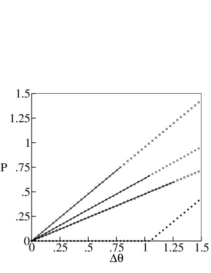
FIG. 3.:

Plot of the probability of Skyrmion formation (average Skyrmion number) vs. $\Delta\theta$ with two domains. Probability of anti-Skyrmions remains zero. Symbols show the results of numerical simulations while the solid line plots show the analytical result from Eq.(22) (plotted only for $\Delta\theta<{\pi\over(\frac{\chi}{\xi}+2)}$). Crosses, open circles, and open squares represent the cases with ($\xi,\chi$) = (1,2), (1,1), and (2,1) respectively. Solid dots show results for winding number 2 Skyrmions for the case with $(\xi,\chi)=(1,2)$.

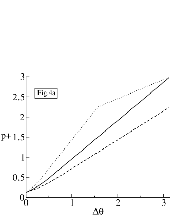
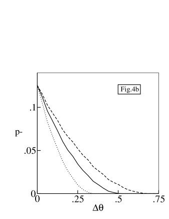
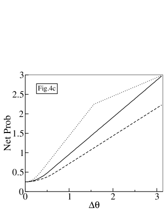
FIG. 4.:

Dotted, solid, and dashed plots show the probabilities of Skyrmion formation (average Skyrmion number) for the choices $(\xi=1,\chi=2),(\xi=1,\chi=1),$, and $(\xi=2,\chi=1)$ respectively. (a) shows the plots for the total probability (i.e., the average numbers) of positive winding Skyrmions. (b) shows plot of anti-windings. (c) shows the sum of (a) and (b) (neglecting the sign of the windings) giving the net average number of Skyrmions and antiSkyrmions.

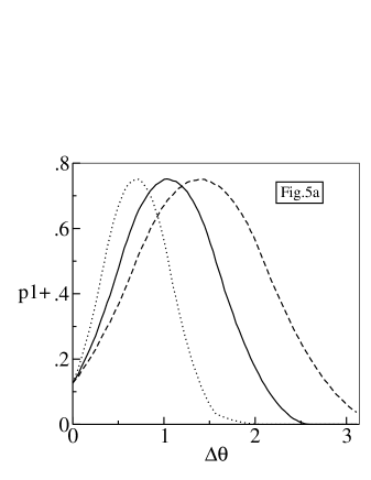
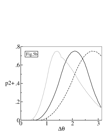
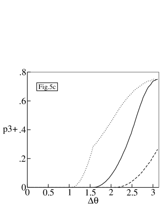
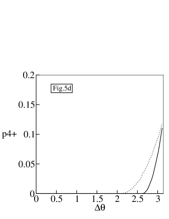
FIG. 5.:

Plots are as shown in Fig.4. (a)-(d) give plots for positive winding Skyrmions with winding 1,2,3, and 4, respectively.

REFERENCES

- [1] A. Vilenkin and E.P.S. Shellard, Cosmic strings and other topological defects, (Cambridge University Press, Cambridge, 1994); A. Gangui, astro-ph/0303504, astro-ph/0110285.
- [2] T.W.B. Kibble, J. Phys. A9 (1976) 1387.
- [3] T.W.B. Kibble, Phys. Rept. 67 (1980) 183.
- [4] W.H. Zurek, Nature 317 (1985) 505; Phys. Rep. 276 (1996) 177.
- [5] A. Rajantie, Int. J. Mod. Phys. A17 (2002) 1.
- [6] P.C. Hendry et al, Nature (London) 368 (1994) 315; V.M.H. Ruutu et al, Nature (London) 382 (1996) 334; M.E. Dodd et al, Phys. Rev. Lett. 81 (1998) 3703; R. Carmi et al, Phys. Rev. Lett. 84 (2000) 4966; see also, G.E. Volovik, Czech. J. Phys. 46 (1996) 3048.
- [7] R. Carmi, E. Polturak, and G. Koren, Phys. Rev. Lett. 84 (2000) 4966; A. Maniv, E. Polturak, and G. Koren, cond-mat/0304359; R.J. Rivers and A. Swarup, cond-mat/0312082; E. Kavoussanaki, R. Monaco, and R.J. Rivers, Phys. Rev. Lett. 85 (2000) 3452; S. Rudaz, A.M. Srivastava and S. Varma, Int. J. Mod. Phys. A14 (1999) 1591.
- [8] I. Chuang, R. Durrer, N. Turok and B. Yurke, Science 251 (1991) 1336; R. Snyder et al. Phys. Rev. A45 (1992) R2169; I. Chuang et al. Phys. Rev. E47 (1993) 3343.
- [9] M.J. Bowick, L. Chandar, E.A. Schiff and A.M. Srivastava, Science 263 (1994) 943.
- [10] S. Digal, R. Ray, and A.M. Srivastava, Phys. Rev. Lett. 83 (1999) 5030; R. Ray and A.M. Srivastava, hep-ph/0110165.
- [11] T.A. DeGrand, Phys. Rev. D30 (1984) 2001; J. Ellis, U. Heinz and H. Kowalski, Phys. Lett. B233 (1989) 223; J. Ellis and H. Kowalski, Nucl. Phys. B327 (1989) 32; Phys. Lett. B214 (1988) 161;
- [12] A. M. Srivastava, Phys. Rev. D43 (1991) 1047.
- [13] J.I. Kapusta and A.M. Srivastava, Phys. Rev. D52 (1995) 2977; see also, J.I. Kapusta and S.M.H. Wong, Phys. Rev. Lett. 86 (2001) 4251; J. Phys. G28 (2002) 1929; J. Dziarmaga and M. Sadzikowski, Phys. Rev. Lett. 82 (1999) 4192.
- [14] M. Stephanov, Prog. Theor. Phys. Suppl. 153 (2004) 139.
- [15] S. Rudaz and A.M. Srivastava, Mod. Phys. Lett. A8 (1993) 1443; M. Hindmarsh, A.C. Davis and R.H. Brandenberger, Phys. Rev. D49 (1994) 1944; R. H. Brandenberger and A.C. Davis, Phys. Lett. B332 (1994) 305; T.W.B. Kibble and A. Vilenkin, Phys. Rev. D52 (1995) 679; J. Borrill, T.W.B. Kibble, T. Vachaspati and A. Vilenkin, Phys. Rev. D52 (1995) 1934.
- [16] M. Hindmarsh and A. Rajantie, Phys. Rev. Lett. 85 (2000) 4660.
- [17] T. Vachaspati, Phys. Rev. D44 (1991) 3723.
- [18] R.F. Alvarez-Estrada and A.G. Nicola, Phys. Lett. B 355 (1995) 288, see also, V. Schon and M. Thies, Phys. Rev. D62 (2000) 096002, K. Ohwa, Phys. Rev. D65 (2002) 085040.
- [19] A.P. Balachandran, Lectures given at Theoretical Advanced Study Inst. in Elementary Particle Physics, New Haven, CT, Published in Yale ASI 1985; I. Zahed and G.E. Brown, Phys. Rept. 142 (1986) 1.
- [20] N. Turok and J. Zadrozny, Phys. Rev. Lett. 65 (1990) 2331; Nucl. Phys. B358 (1991) 471; D. Grigoriev, M. Shaposhnikov, and N. Turok, Phys. Lett. B275 (1992) 395.