Supersymmetric Grandunification and Fermion Masses

Abstract

A short review of the status of supersymmetric grand unified theories and their relation to the issue of fermion masses and mixings is given.

Abstract

We consider branes as “points” in an infinite dimensional brane space ${\cal M}$ with a prescribed metric. Branes move along the geodesics of ${\cal M}$. For a particular choice of metric the equations of motion are equivalent to the well known equations of the Dirac-Nambu-Goto branes (including strings). Such theory describes “free fall” in ${\cal M}$-space. In the next step the metric of ${\cal M}$-space is given the dynamical role and a corresponding kinetic term is added to the action. So we obtain a background independent brane theory: a space in which branes live is ${\cal M}$-space and it is not given in advance, but comes out as a solution to the equations of motion. The embedding space (“target space”) is not separately postulated. It is identified with the brane configuration.

Abstract

We review present information on cosmological neutrinos, and more generally on relativistic degrees of freedom at the Cosmic Microwave Background formation epoch, in view of the recent results of WMAP collaborations on temperature anisotropies of the CMB, as well as of recent detailed analysis of Primordial Nucleosynthesis.

Abstract

The quark-lepton mass problem and the ideas of mass protection are reviewed. The Multiple Point Principle is introduced and used within the Standard Model to predict the top quark and Higgs particle masses. We discuss the lightest family mass generation model, in which all the quark mixing angles are successfully expressed in terms of simple expressions involving quark mass ratios. The chiral flavour symmetry of the family replicated gauge group model is shown to provide the mass protection needed to generate the hierarchical structure of the quark-lepton mass matrices.

Abstract

The application of quantum theory to gravity is beset with many technical and conceptual problems. After a short tour d’horizon of recent attempts to master those problems by the introduction of new approaches, we show that the aim, a background independent quantum theory of gravity, can be reached in a particular area, 2d dilaton quantum gravity, without any assumptions beyond standard quantum field theory.

Abstract

In M-theory vacua with vanishing 4-form $F_{(4)}$, one can invoke the ordinary Riemannian holonomy $H\subset{\rm SO}(10,1)$ to account for unbroken supersymmetries $n=1$, 2, 3, 4, 6, 8, 16, 32. However, the generalized holonomy conjecture, valid for non-zero $F_{(4)}$, can account for more exotic fractions of supersymmetry, in particular $16<n<32$. The conjectured holonomies are given by ${\cal H}\subset{\cal G}$ where ${\cal G}$ are the generalized structure groups ${\cal G}={\rm SO}(d-1,1)\times G(spacelike)$, ${\cal G}={\rm ISO}(d-1)\times G(null)$ and ${\cal G}={\rm SO}(d)\times G(timelike)$ with $1\leq d<11$. For example, $G(spacelike)={\rm SO}(16)$, $G(null)=[{\rm SU}(8)\times{\rm U}(1)]\ltimes{\mathbb{R}}^{56}$ and $G(timelike)={\rm SO}^{*}(16)$ when $d=3$. Although extending spacetime symmetries, there is no conflict with the Coleman-Mandula theorem. The holonomy conjecture rules out certain vacua which are otherwise permitted by the supersymmetry algebra.

Abstract

In previous articles it has been argued that a differential calculus over a noncommutative algebra uniquely determines a gravitational field in the commutative limit and that there is a unique metric which remains as a commutative ‘shadow’. Some examples were given of metrics which resulted from a given algebra and given differential calculus. Here we aboard the inverse problem, that of constructing the algebra and the differential calculus from the commutative metric. As an example a noncommutative version of the Kasner metric is proposed which is periodic.

Abstract

We put forward the multiple point principle as a fine-tuning mechanism that can explain why some of the parameters of the standard model have the values observed experimentally. The principle states that the parameter values realized in Nature coincide with the surface (e.g. the point) in the action parameter space that lies in the boundary that separates the maximum number of regulator-induced phases (e.g., the lattice artifact phases of a lattice gauge theory). We argue that a mild form of non-locality - namely that embodied in allowing diffeomorphism invariant contributions to the action - seems to be needed for some fine-tuning problems. We demonstrate that the multiple point principle solution to fine-tuning has the very special property of avoiding the paradoxes that can arise in the presence of non-locality. The non-renormalizability of gravity suggests — in a manner reminiscent of baby universe theory — the presence of non-local effects without which the phenomenologically observed high degree of flatness of spacetime would seem mysterious. In our picture, different vacuum states are realized in different spacetime regions of the cosmological history.

Abstract

The extension of the Veneziano-Yankielowicz effective Lagrangian with terms including covariant derivatives is discussed. This extension is important to understand glue-ball dynamics of the theory. Though the superpotential remains unchanged, the physical spectrum exhibits completely new properties.

Abstract

We summarize our recent results of studying five-dimensional Kasner cosmologies in a time-dependent Calabi-Yau compactification of M-theory undergoing a topological flop transition. The dynamics of the additional states, which become massless at the transition point and give rise to a scalar potential, helps to stabilize the moduli and triggers short periods of accelerated cosmological expansion.

Abstract

The violation of Lorentz symmetry can arise in a variety of approaches to fundamental physics. For the description of the associated low-energy effects, a dynamical framework known as the Standard-Model Extension has been developed. This talk gives a brief review of the topic focusing on Lorentz violation through varying couplings.

Abstract

We analyse the curvaton scenario in the context of supersymmetry. Supersymmetric theories contain many scalars, and therefore many curvaton candidates. To obtain a scale invariant perturbation spectrum, the curvaton mass should be small during inflation $m\ll H$. This can be achieved by invoking symmetries, which suppress the soft masses and non-renormalizable terms in the potential. Other model-independent constraints on the curvaton model come from nucleosynthesis, gravitino overproduction, and thermal damping. The curvaton can work for masses $m\stackrel{{\scriptstyle>}}{{{}_{\scriptstyle\sim}}}10^{4}{\,\mbox{GeV}}$, and very small couplings (e.g. $h\stackrel{{\scriptstyle<}}{{{}_{\scriptstyle\sim}}}10^{-6}$ for $m\stackrel{{\scriptstyle<}}{{{}_{\scriptstyle\sim}}}10^{8}{\,\mbox{GeV}}$).

Abstract

We review the original result we have obtained in the analysis of the breaking of perturbative unitarity in space-time noncommutative field theories in the light of their relations to D-branes in electric backgrounds

Abstract

We review recently developed cohomological methods relating to the study of supersymmetric theories and their deformations.

1 Why Grandunification?

There are essentially three reasons for trying to build grand unified theories (GUTs) beyond the standard model (SM).

• why should strong, weak and electromagnetic couplings in the SM be so different despite all corresponding to gauge symmetries?

• there are many disconnected matter representations in the SM (3 families of $L$, $e^{c}$, $Q$, $u^{c}$, $d^{c}$)

• quantization of electric charge (in the SM model there are two possible explanations - anomaly cancellation and existence of magnetic monopoles - both are naturally embodied in GUTs)

2 How to check a GUT?

I will present here a very short review of some generic features, predictions and drawbacks of GUTs. Details of some topics will be given in the next section.

2.1 Gauge coupling unification

This is of course a necessary condition for any GUT to work. As is well known, the SM field content plus the desert assumption do not lead to the unification of the three gauge couplings. However, the idea of low-energy supersymmetry (susy), i.e. the minimal supersymmetric standard model (MSSM) instead of the SM at around TeV and again the assumption of the desert gives a quite precise unification of gauge couplings at $M_{GUT}\approx 10^{16}$ GeV Dimopoulos:1981yj . Clearly there is no a-priori reason for three functions to cross in one point, so this fact is a strong argument for supersymmetry. One gets two bonuses for free in this case. First, the hierarchy problem gets stabilized, although not really solved, since the famous doublet-triplet (DT) problem still remains. Secondly, at least in principle one can get an insight into the reasons for the electroweak symmetry breaking: why the Higgs (other bosons in MSSM) mass squared is negative (positive) at low energy Inoue:1982pi .

2.2 Fermion masses and mixings

Although GUTs are not theories of flavour, they bring constraints on the possible Yukawas. In the MSSM the Yukawa sector is given by

$$W_{Y}=HQ^{T}Y_{U}u^{c}+\overline{H}Q^{T}Y_{D}d^{c}+\overline{H}L^{T}Y_{E}e^{c}\;,$$ (1)

and the complex $3\times 3$ generation matrices $Y_{U,D,E}$ are arbitrary. However, in a GUT the matter fields $Q$, $L$, $u^{c}$, $d^{c}$, $e^{c}$ fields live together in bigger representations, so one expects relations between quark and lepton Yukawa matrices.

Take for example the SO(10) GUT. All the MSSM matter fields of each generation live in the same representation, the $16$ dimensional spinor representation, which contains and thus predicts also the right-handed neutrino. At the same time the minimal Higgs representation, the $10$ dimensional representation contains both doublets $H$ and $\overline{H}$ of the MSSM (plus one color triplet and one antitriplet). The only renormalizable SO(10) invariant one can write down is thus

$$W_{Y}=10_{H}16Y_{10}16\;,$$ (2)

which is however too restrictive, since it gives on top of the well satisfied (for large $\tan{\beta}$) relation $y_{b}=y_{\tau}=y_{t}$ for the third generation, the much worse predictions for the first two generations ($y_{s}=y_{\mu}=y_{c}$ and $y_{d}=y_{e}=y_{u}$) and no mixing ($\theta_{c}=0$) at all.

How to improve the fit? Let us mention two possibilities:

(1) Introduce new Higgs representations: although another $10_{H}$ can help with the mixing, the experimentally wrong relations $m_{d}=m_{e}$ and $m_{s}=m_{\mu}$ still occur, because the two bi-doublets in the two $10_{H}$ leave invariant the Pati-Salam SO(6)=SU(4)_C, so the leptons and quarks are still treated on the same footing. So the idea to pursue is to introduce bidoublets which transform nontrivially under the Pati-Salam SU(4) color. This can be done for example by introducing a $\overline{126}_{H}$, which couples to matter as $\Delta W_{Y}=\overline{126}_{H}16Y_{126}16$ and which gets a nontrivial vev in the $(2,2,15)_{H}$ SU(3) color singlet direction Lazarides:1980nt ; Babu:1992ia .

(2) Another possibility is to include the effects of nonrenormalizable operators. These operators can cure the problem and at the same time ease the proton decay constraints. The drawback is the loss of predictivity.

2.3 Proton decay

This issue is connected to

(1) R-parity. It is needed to avoid fast proton decay. At the nonrenormalizable level one could for example have terms leading to R-parity violation of the type $16^{3}16_{H}/M_{Pl}$. For this reason it is preferable to use the $126_{H}$ representation instead of the $16_{H}$. It is possible to show that such a SO(10) with $126_{H}$ has an exact R-parity Aulakh:1997ba at all energies without the introduction of further symmetries.

(2) DT splitting problem: Higgs SU(2)_L doublets and SU(3)_C triplets live usually in the same GUT multiplet; but while the SU(2)_L doublets are light ($\approx M_{W}\ll M_{GUT}$), the SU(3)_C triplets should be very heavy ($\geq M_{GUT}$) to avoid a too fast proton decay. For example, the proton lifetime in susy is proportional to $M_{T}^{2}$, which can give a lower limit to the triplet mass Hisano:1992jj , although this limit depends on the yet unknown supersymmetry breaking sector Bajc:2002bv .

The solutions to the DT problem depend on the gauge group considered, but in general models that solve it are not minimal and necessitate of additional Higgs sectors. For example the missing partner mechanism Masiero:1982fe in SU(5) needs at least additional $75_{H}$, $50_{H}$ and $\overline{50}_{H}$ representations. The same is true for the missing vev mechanism in SO(10) Dimopoulos:xm , where the $45_{H}$ and extra $10_{H}$ Higgses must be introduced. Also the nice idea of GIFT (Goldstones Instead of Fine Tuning) Berezhiani:1995sb can be implemented only by complicated models, while discrete symmetries for this purpose can be used with success only in connection with non-simple gauge groups Barbieri:1994jq . Of course, although not very natural, any GUT can ”solve” the problem phenomenologically, i.e. simply fine-tuning the model parameters.

Clearly, whatever is the solution to the DT problem, the proton lifetime depends in a crucial (powerlike) way on the triplet mass. And this mass can be difficult to determine from the gauge coupling unification condition even in specific models because of the unknown model parameters Bachas:1995yt or use of high representations Dixit:1989ff . On top of this there can be large uncertainties in the triplet Yukawa couplings Dvali:1992hc . All this, together with the phenomenologically completely unknown soft susy breaking sector, makes unfortunately proton decay not a very neat probe of supersymmetric grandunification Bajc:2002bv . Of course, if for some reason the DT mechanism is so efficient to make the $d=6$ operators dominant (for a recent analysis in some string-inspired models see Friedmann:2002ty ), then the situation could be simpler to analyse Mohapatra:yj , although many uncertainties due to fermion mixing matrices still exist in realistic nonminimal models Nandi:1982ew . Unfortunately there is little hope to detect proton decay in this case, unless $M_{GUT}$ is lower than usual Aulakh:2000sn .

2.4 Magnetic monopoles

Since magnetic monopoles are too heavy to be produced in colliders, the only hope is to find them as relics from the cosmological GUT phase transitions. Their density however strongly depends on the cosmological model considered. Unfortunately, the Rubakov-Callan effect Rubakov:fp leads to the non observability of GUT monopoles, at least in any foreseeable future. Namely, these monopoles are captured by neutron stars and the resulting astrophysical analyses Freese:1983hz limits the monopole flux at earth twelve orders of magnitude below the MACRO limit Giacomelli:2003yu .

This is very different from the situation in the Pati-Salam (PS) theory. Even in the minimal version the PS scale can be much lower than the GUT scale Melfo:2003xi , as low as $10^{10}$ GeV. the resulting monopoles are then too light to be captured by neutron stars and their flux is not limited due to the Rubakov-Callan effect. Furthermore, MACRO results are not applicable for such light monopoles Giacomelli:2003yu .

2.5 Low energy tests

There are many different possible tests at low-energy, like for example the flavour changing neutral currents (see for example Barbieri:1994pv ) or the electric dipole moments Masina:2003iz . In the latter case the exact value of the triplet mass is much less important than in proton decay, but the uncertainties due to the susy breaking sector are still present. In some of these tests like neutron-antineutron oscillation we can get positive signatures only for specific models due to very high dimensional operators involved Babu:2001qr .

3 Fermion masses and mixings

The regular pattern of 3 generations suggests some sort of flavour symmetry.

One way, and the most ambitious one, is to consider the flavour symmetry group as part (subgroup) of the grand unified gauge symmetry (described by a simple group). In such an approach all three generations come from the same GUT multiplet. For example, in SU(8) the 216 dimensional representation gets decomposed under its SU(5) subgroup into three copies (generations) of $\overline{5}$ and $10$ with additional SU(5) multiplets. Similarly, in the SO(18) GUT, the 256 dimensional spinorial representation is nothing else than 8 generations of $(16+\overline{16})$ in the SO(10) language. The problem in all these theories is what to do with all the extra light particles Wilczek:1981iz .

Another possibility is to consider the product of the flavour (or, in general, extra) symmetry with the GUT symmetry (simple) group. In the context of SO(10) GUTs most of them use small representations for the Higgses, like $16_{H}$, $\overline{16}_{H}$ and $45_{H}$. The philosphy is to consider all terms allowed by symmetry, also nonrenormalizable. The DT problem can be naturally solved by some version of the missing vev mechanism, which however means that many multiplets are usually needed. Such models are quite successfull Albright:2000sz , although the assumed symmetries are a little bit ad-hoc. There is also a huge number of different models with almost arbitrary flavour symmetry group, but unfortunately there is no room to describe them here (see for example the recent review Chen:2003zv ).

What we will consider in the following is instead a SO(10) GUT with no extra symmetry at all. We want to see how far we can go with just the grand unified gauge symmetry alone. To ensure automatic R-parity, we are forced not to use the $16_{H}$ and $\overline{16}_{H}$ Higgses, but instead a pair of $126_{H}$ and $\overline{126}_{H}$ (5 index antisymmetric representations, one self-dual, the other anti-self-dual; both of them are needed in order not to break susy at a large scale). In fact under R-parity the bosons of $16$ are odd, while those of $126$ are even, since

$$R=(-1)^{3(B-L)+2S}$$ (3)

Mohapatra:su , and the relevant vev in the SU(5) singlet directions have $B-L=1$ for $16_{H}$ ($\nu^{c}$), while it has $B-L=2$ for $126$ (the mass of $\nu^{c}$).

So the rules of the game are: stick to renormalizable operators only, consider SO(10) as the only symmetry of the model, take the minimal number of multiplets (it does not mean the minimal number of fields!) that is able to give the correct symmetry breaking pattern SO(10)$\to$SU(3)$\times$SU(2)$\times$U(1). Such a theory is given by Clark:ai (see however Aulakh:1982sw for a similar approach): on top of the usual three generations of $16$ dimensional matter fields, it contains four Higgs representations: $10_{H}$, $126_{H}$, $\overline{126}_{H}$ and $210_{H}$ (4 index antisymmetric). It has been shown recently Aulakh:2003kg that this theory is also the minimal GUT, i.e. it has the minimal number of model parameters, being still perfectly realistic (not in contradiction with any experiment).

As we have seen, the $\overline{126}_{H}$ multiplet is needed both to help the $10_{H}$ multiplet in fitting the fermion masses and mixings, and for giving the mass to the right-handed neutrino without explicitly breaking R-parity. Let us now see, why the $210_{H}$ representation is needed.

The Yukawa sector is given by

$$W_{Y}=10_{H}16Y_{10}16+\overline{126}_{H}16Y_{126}16\;.$$ (4)

The fields decompose under the SU(2)${}_{L}\times$SU(2)${}_{R}\times$SU(4)_C subgroup as

$$10_{H} = (2,2,1)+(1,1,6)\;,$$ (5)

$$16 = (2,1,4)+(1,2,\overline{4})\;,$$ (6)

$$\overline{126}_{H} = (1,3,10)+(3,1,\overline{10})+(2,2,15)+(1,1,6)\;.$$ (7)

The right-handed neutrino $\nu^{c}$ lives in $(1,2,\overline{4})$ of $16$, so it can get a large mass only through the second term in (4):

$$M_{\nu_{R}}=\langle(1,3,10)_{\overline{126}}\rangle Y_{126}\;,$$ (8)

where $\langle(1,3,10)\rangle$ is the scale of the SU(2)_R symmetry breaking $M_{R}$, which we assume to be large, ${\cal O}(M_{GUT})$.

In order to get realistic masses we need

$$\langle(2,2,1)_{10}\rangle = \begin{pmatrix}v_{10}^{d}&0\cr 0&v_{10}^{u}\cr\end{pmatrix}\neq 0\;,$$ (9)

$$\langle(2,2,15)_{\overline{126}}\rangle = \begin{pmatrix}v_{126}^{d}&0\cr 0&v_{126}^{u}\cr\end{pmatrix}\neq 0\;,$$ (10)

which contribute to the light fermion masses as

$$M_{U} = v_{10}^{u}Y_{10}+v_{126}^{u}Y_{126}\;,$$ (11)

$$M_{D} = v_{10}^{d}Y_{10}+v_{126}^{d}Y_{126}\;,$$ (12)

$$M_{\nu_{D}} = v_{10}^{u}Y_{10}-3v_{126}^{u}Y_{126}\;,$$ (13)

$$M_{E} = v_{10}^{d}Y_{10}-3v_{126}^{d}Y_{126}\;.$$ (14)

The factor of $-3$ for leptons in the contribution from $\overline{126}_{H}$ comes automatically from the fact that the SU(3)_C singlet in the adjoint $15$ of SU(4)_C is in the $B-L$ direction diag$(1,1,1,-3)$. This is clearly absent in the contribution from $10_{H}$, which is a singlet under the full SU(4)_C.

The light neutrino mass comes through the famous see-saw mechanism Mohapatra:1979ia . From

$$W={1\over 2}\nu^{cT}M_{\nu_{R}}\nu^{c}+\nu^{cT}M_{\nu_{D}}\nu_{L}+...$$ (15)

one can integrate out the heavy right-handed neutrino $\nu^{c}$ obtaining the effective mass term for the light neutrino states $M_{N}=-M_{\nu_{D}}^{T}M_{\nu_{R}}^{-1}M_{\nu_{D}}$. As we will now see, there is another contribution in our minimal model.

(1) We saw that both $\langle(2,2,1)_{10}\rangle$ and $\langle(2,2,15)_{126}\rangle$ need to be nonzero and obviously ${\cal O}(M_{W})$. With $10_{H}$, $126_{H}$ and $\overline{126}_{H}$ Higgses one can write only two renormalizable invariants:

$$W_{H}={1\over 2}M_{10}10_{H}^{2}+M_{126}126_{H}\overline{126}_{H}\;,$$ (16)

where $M_{10},M_{126}\approx{\cal O}(M_{GUT})$ or larger due to proton decay constraints. So the mass term looks like

$${1\over 2}(10_{H},126_{H},\overline{126}_{H})\begin{pmatrix}M_{10}&0&0\cr 0&0&M_{126}\cr 0&M_{126}&0\cr\end{pmatrix}\begin{pmatrix}10_{H}\cr 126_{H}\cr\overline{126}_{H}\cr\end{pmatrix}\;.$$ (17)

Clearly all the doublets have a large positive mass, so their vev must be zero. Even fine-tuning cannot solve the DT problem in this case. So the idea to overcome this obstacle is to mix in some way $10_{H}$ with $\overline{126}_{H}$ ($126_{H}$), and after that fine-tune to zero one combination of doublet masses. So the new mass matrix should look something like

$$\begin{pmatrix}M_{10}&x&y\cr x&0&M_{126}\cr y&M_{126}&0\cr\end{pmatrix}$$ (18)

with $x,y$ denoting such mixing. The light Higgs doublets will thus be linear combinations of the fields in $(2,2,1)_{10}$ and $(2,2,15)_{126_{H},\overline{126}_{H}}$ and this will get a nonzero vev after including the soft susy breaking masses.

(2) The minimal representation that can mix $10$ and $\overline{126}$ is $210$, as can be seen from $10\times\overline{126}=210+1050$. $210$ is a 4 index antisymmetric SO(10) representation, which decomposes under the Pati-Salam subgroup as

$$210=(1,1,1)+(1,1,15)+(1,3,15)+(3,1,15)+(2,2,6)+(2,2,10)+(2,2,\overline{10})\;.$$ (19)

Of course one can now add other renormalizable terms to (16), and all such new terms are (in a symbolic notation)

$$\Delta W_{H}=210_{H}^{3}+210_{H}^{2}+210_{H}126_{H}\overline{126}_{H}+210_{H}10_{H}126_{H}+210_{H}10_{H}\overline{126}_{H}\;.$$ (20)

The last two terms are exactly the ones needed for the mixings between $10_{H}$ and $126_{H}$ ($\overline{126}_{H}$), i.e. contributions to $x,y$ in (18). It is possible to show that $W_{H}+\Delta W_{H}$ are just enough for SO(10)$\to$SM. In the case of single-step breaking one thus has

$$\langle(1,1,1)_{210}\rangle \approx \langle(1,1,15)_{210}\rangle\approx\langle(1,3,15)_{210}\rangle\approx$$

$$\langle(1,3,\overline{10})_{126}\rangle \approx \langle(1,3,10)_{\overline{126}}\rangle\approx M_{GUT}\;.$$ (21)

(3) Now however there are five bidoublets that mix, since $(2,2,10)$ and $(2,2,\overline{10})$ from $210_{H}$ also contribute. To be honest, there is only one neutral component in each of these last two bidoublets, since their $B-L$ equals $\pm 2$, so the final mass matrix for the Higgs doublets is $4\times 4$. Only one eigenvalue of this matrix needs to be zero, and this can be achieved by fine-tuning. Each of the two Higgs doublets of the MSSM is thus a linear combination of 4 doublets, each of which has in general a vev of order ${\cal O}(M_{W})$:

$$\langle(2,2,1)_{10}\rangle \approx \langle(2,2,15)_{\overline{126}}\rangle\approx M_{W}\approx$$ (22)

$$\langle(2,2,15)_{126}\rangle \approx \langle(2,2,10)_{210}\rangle\approx\langle(2,2,\overline{10})_{210}\rangle\;.$$

This mixing is nothing else than the susy version of Lazarides:1980nt ; Babu:1992ia .

(4) Due to all these bidoublet vevs, a SU(2)_L triplet will also get a tiny but nonzero vev. Applying the susy constraint $F_{(3,1,10)_{126}}=0$ to

$$W=M_{126}(3,1,10)_{126}(3,1,\overline{10})_{\overline{126}}+(2,2,1)_{10}(2,2,\overline{10})_{210}(3,1,10)_{126}+...$$ (23)

one immediately gets

$$\langle(3,1,\overline{10})_{\overline{126}}\approx{\langle(2,2,1)_{10}\rangle\langle(2,2,\overline{10})_{210}\rangle\over M_{126}}\approx{M_{W}^{2}\over M_{GUT}}\neq 0\;.$$ (24)

This effect is just the susy version of Magg:1980ut .

(5) Since $\nu$ lives in $(2,1,4)_{16}$, the second term in (4) gives among others also a term $(3,1,\overline{10})_{\overline{126}}(2,1,4)_{16}Y_{126}(2,1,4)_{16}$, which contributes to the light neutrino mass. So all together one gets for the light neutrino mass ($c$ is a model dependent dimensionless parameter)

$$M_{N}=-M_{\nu_{D}}^{T}M_{\nu_{R}}^{-1}M_{\nu_{D}}+c{M_{W}^{2}\over M_{GUT}}Y_{126}\;.$$ (25)

The first term is called the type I (or canonical) see-saw and is mediated by the SU(2)_L singlet $\nu^{c}$, while the second is the type II (or non-canonical) see-saw, and is mediated by the SU(2)_L triplet.

Equations (11), (12), (13), (14), (8) and (25) are all we need in the fit of known fermion masses and mixings and predictions of the unknown ones. A possible procedure is first to trade the matrices $Y_{10}$ and $Y_{126}$ for $M_{U}$ and $M_{D}$. The remaining freedom in $M_{U}$ and $M_{D}$ is still enough to fit $M_{E}$. But then some predictions in the neutrino sector are possible. For this sector we need to reproduce the experimental results $(\theta_{l})_{12,23}\gg(\theta_{q})_{12,23}$ and $(\theta_{l})_{13}$ small. The degree of predictivity of the model however depends on the assumptions regarding the see-saw and on the CP phases.

The first approach was to consider models in which type I dominates. It was shown that such models predict a small atmospheric neutrino mixing angle $\theta_{atm}=(\theta_{l})_{23}$ if the CP phases are assumend to be small Babu:1992ia ; Lee:1994je . On the other hand, a large atmospheric neutrino mixing angle can be also large, if one allows for arbitrary CP phases and fine-tune them appropriately Matsuda:2001bg .

A completely different picture emerges if one assumes that type II see-saw dominates. In this case even without CP violation one can naturally have a large atmospheric neutrino mixing angle, as has been first emphasized for the approximate case of second and third generations only in Bajc:2001fe ; Bajc:2002iw . In the three generation case the same result has been confirmed Goh:2003sy . On top of this, a large solar neutrino mixing angle and a prediction of $U_{e3}\approx 0.15\pm 0.01$ (close to the upper experimental limit) have been obtained Goh:2003sy . Even allowing for general CP violation does not invalidate the above results: although the error bars are larger, the general picture of large atmospheric and solar neutrino mixing angles and small $U_{e3}$ still remains valid Goh:2003hf .

It is possible to understand why type II see-saw gives so naturally a large atmospheric mixing angle. In type II the light neutrino mass matrix (25) is proportional to $Y_{126}$. From (12) and (14) one can easily find out, that $Y_{126}\propto M_{D}-M_{E}$, from which one gets Brahmachari:1997cq

$$M_{N}\propto M_{D}-M_{E}\;.$$ (26)

As a warm-up let us take the approximations of just (a) two generations, the second and the third, (b) neglect the masses of the second generation with respect of the third ($m_{s,\mu}\ll m_{b,\tau}$) and (c) assume that $M_{D}$ and $M_{E}$ has small mixings (this amounts to say, that in the basis of diagonal charged lepton mass, the smallness of the $({\theta_{q}})_{23}=\theta_{cb}$ is not caused by accidental cancellation of two large numbers). In this approximate set-up one gets

$$M_{N}\propto\begin{pmatrix}0&0\cr 0&m_{b}-m_{\tau}\cr\end{pmatrix}\;.$$ (27)

This is, in type II see-saw there is a correspondence between the large atmospheric angle and $b-\tau$ unification Bajc:2002iw .

Remember here that $b-\tau$ Yukawa unification is no more automatic, since we have also $\overline{126}_{H}$ Higgs on top of the usual $10_{H}$. It is however quite well satisfied phenomenologically.

One can do better: still take $m_{s,\mu}\approx 0$, but allow a nonzero quark mixing. In this case the atmospheric mixing angle is

$$\tan{2\theta_{atm}}={\sin{2\theta_{cb}}\over 2\sin^{2}{\theta_{cb}}-{m_{b}-m_{\tau}\over m_{b}}}\;.$$ (28)

Since $\theta_{cb}\approx{\cal O}(10^{-2})$, one again finds out the correlation between the large atmospheric mixing angle and $b-\tau$ unification at the GUT scale.

The result can be confirmed of course also for finite $m_{s,\mu,c}$, although not in a so simple and elegant way.

Of course there are many other models that predict and/or explain a large atmospheric mixing angle (for a recent review see for example King:2003jb ). What is surprising here is, however, that no other symmetry except the gauge SO(10) is needed whatsoever.

4 The minimal model

As we saw in the previos section, one can correctly fit the known masses and mixings, get some understanding of the light neutrino mass matrix, and obtain some new predictions. What we would like to show here is that the model considered above has less number of model parameters than any other GUT, and can be then called the minimal realistic supersymmetric grand unified theory (even more minimal than SU(5)!) Aulakh:2003kg .

The Higgs sector described by (16) and (20) contains $10$ real parameters ($7$ complex parameters minus four phase redefinitions due to the four complex Higgs multiplets involved). The Yukawa sector (4) has two complex symmetric matrices, one of which can be always made diagonal and real by a unitary transformation of $16$ in generation space. So what remains are $15$ real parameters. There is on top of this also the gauge coupling, so all together 26 real parameters in the supersymmetric sector of renormalizable SO(10) GUT with three copies of matter 16 and Higgses in the representations $10_{H}$, $126_{H}$, $\overline{126}_{H}$ and $210_{H}$. We will not consider the susy breaking sector, since this is present in all supersymmetric theories, GUTs or not.

Before comparing with other GUTs, for example SU(5), let us count the number of model parameters in MSSM. There are 6 quark masses, 3 quark mixing angles, 1 quark CP phase, 6 lepton masses, 3 lepton mixing angles and 3 lepton CP phases (assuming Majorana neutrinos). On top of this, there are 3 gauge couplings and the real $\mu$ parameter. Thus, all together, again 26 real parameters. They are however distributed differently, so that in the Yukawa sector there are only 15 parameters in our minimal SO(10) GUT, which has to fit 22 MSSM (at least in principle) measurable low-energy parameters. Although in this fitting also few vevs that contain parameters from the Higgs and susy breaking sector play a role, the minimal SO(10) is nevertheless predictive.

One can play with other SO(10) models: the renormalizable ones need more representations and thus have more invariants, while the nonrenormalizable ones (those that use $16_{H}$ instead of $126_{H}$) have a huge number of invariants, some of which must be very small due to R-symmetry constraints. Of course, with some extra discrete, global or local symmetry, one can forbid these unpleasant and dangerous terms, remaining even with a small number of parameters, but as we said, this is not allowed in our scheme, in which we want to obtain as much information as possible just from GUT gauge symmetry (and renormalizability).

The simplicity of the minimal renormalizable supersymmetric SU(5) looks as if the number of parameters here could be smaller than in our previous example. What however gives a large number of parameters is the fact, that SU(5) is not particularly suitable for the neutrino sector. In fact, one can play and find out, that the minimal SU(5) with nonzero neutrino masses is obtained adding the two index symmetric $15_{H}$ and $\overline{15}_{H}$, and the number of model parameters comes out to be 39, i.e. much more than in the minimal SO(10).

5 Conclusion

Before talking about flavour symmetries it is important first to know, what we can learn from just pure GUTs. The minimal GUT is a SO(10) gauge theory with representations $10_{H}$, $126_{H}$, $\overline{126}_{H}$, $210_{H}$ and three generations of $16$. Such a realistic theory is renormalizable and no extra symmetries are needed. It can fit the fermion masses and mixings, and can give an interesting relation between $b-\tau$ Yukawa unification and large atmospheric mixing angle. It has a testable prediction for $U_{e3}$. Due to the large representations involved, it is not asymptotically free, which means that it predicts some new physics below $M_{Pl}$.

There are many virtues of this minimal GUT. As in any SO(10) all fermions of one generation are in the same representation and the right-handed neutrino is included automatically, thus explaining the tiny neutrino masses by the see-saw mechanism. Employing $126_{H}$ instead of $16_{H}$ to break $B-L$ maintains R-symmetry exact at all energies. It is economical, it employs the minimal number of multiplets and parameters, and thus it is maximally predictive. It gives a good fit to available data and gives a framework to better understand the differences between the mixings in the quark and lepton sectors.

There are of course also some drawbacks. First, in order to maintain predictivity, one must believe in the principle of renormalizability, although the suppressing parameter in the expansion $M_{GUT}/M_{Planck}$ is not that small. Of course, in supersymmetry these terms can be small and stable, but this choice is not natural in the ’t Hooft sense. Second, the DT splitting problem is here, and attempts to solve it require more fields Lee:1993jw . Finally, usually it is said that $126$ dimensional representations are not easy to get from superstring theories, although we are probably far from a no-go theorem.

There are many open questions to study in the context of the minimal SO(10), let me mention just few of them. First, proton decay: although it is generically dangerous, it is probably still possible to fit the data with some fine-tuning of the model parameters as well as of soft susy breaking terms. An interesting question is whether the model is capable of telling us which type of see-saw dominates. If it is type I or mixed, can it still give some testable prediction for $U_{e3}$? Also, gauge coupling unification should be tested in some way, although large threshold corrections could be nasty Dixit:1989ff . And finally, is there some hope to solve in this context or minimal (but still predictive) extensions the doublet-triplet splitting problem?

*General Principles of Brane Kinematics and Dynamics Matej Pavšič

6 Introduction

Theories of strings and higher dimensional extended objects, branes, are very promising in explaining the origin and interrelationship of the fundamental interactions, including gravity. But there is a cloud. It is not clear what is a geometric principle behind string and brane theories and how to formulate them in a background independent way. An example of a background independent theory is general relativity where there is no preexisting space in which the theory is formulated. The dynamics of the 4-dimensional space (spacetime) itself results as a solution to the equations of motion. The situation is sketched in Fig.1. A point particle traces a world line in spacetime whose dynamics is governed by the Einstein-Hilbert action. A closed string traces a world tube, but so far its has not been clear what is the appropriate space and action for a background independent formulation of string theory.

Figure 1: To point particle there corresponds the Einstein-Hilbert action in spacetime. What is a corresponding space and action for a closed string?

Here I will report about a formulation of string and brane theory (see also ref. book ) which is based on the infinite dimensional brane space ${\cal M}$. The “points” of this space are branes and their coordinates are the brane (embedding) functions. In ${\cal M}$-space we can define the distance, metric, connection, covariant derivative, curvature, etc. We show that the brane dynamics can be derived from the principle of minimal length in ${\cal M}$-space; a brane follows a geodetic path in ${\cal M}$. The situation is analogous to the free fall of an ordinary point particle as described by general relativity. Instead of keeping the metric fixed, we then add to the action a kinetic term for the metric of ${\cal M}$-space and so we obtain a background independent brane theory in which there is no preexisting space.

7 Brane space ${\cal M}$ (brane kinematics)

We will first treat the brane kinematics, and only later we will introduce a brane dynamics. We assume that the basic kinematically possible objects are $n$-dimensional, arbitrarily deformable branes ${\cal V}_{n}$ living in an $N$-dimensional embedding (target) space $V_{N}$. Tangential deformations are also allowed. This is illustrated in Fig. 2. Imagine a rubber sheet on which we paint a grid of lines. Then we deform the sheet in such a way that mathematically the surface remains the same, nevertheless the deformed object is physically different from the original object.

Figure 2: Examples of tangentially deformed membranes. Mathematically the surface on the left and is the same as the surface on the right. Physically the two surfaces are different.

We represent ${\cal V}_{n}$ by functions $X^{\mu}(\xi^{a})~{},~{}~{}\mu=0,1,...,N-1$, where $\xi^{a},~{}a=0,1,2,...,n-1$ are parameters on ${\cal V}_{n}$. According the assumed interpretation, different functions $X^{\mu}(\xi^{a})$ can represent physically different branes. That is, if we perform an active diffeomorphism $\xi^{a}\rightarrow\xi^{\prime a}=f^{a}(\xi)$, then the new functions $X^{\mu}(f^{a}(\xi))=X^{\prime\mu}(\xi)$ represent a physically different brane ${\cal V}^{\prime}_{n}$. For a more complete and detailed discussion see ref. book .

The set of all possible ${\cal V}_{n}$ forms the brane space ${\cal M}$. A brane ${\cal V}_{n}$ can be considered as a point in ${\cal M}$ parametrized by coordinates $X^{\mu}(\xi^{a})\equiv X^{\mu(\xi)}$ which bear a discrete index $\mu$ and $n$ continuous indices $\xi^{a}$. That is, $\mu(\xi)$ as superscript or subscript denotes a single index which consists of the discrete part $\mu$ and the continuous part $(\xi)$.

In analogy with the finite-dimensional case we can introduce the distance $\mbox{\rm d}\ell$ in the infinite-dimensional space ${\cal M}$:

$${\mbox{\rm d}}{\ell}^{2}=\int{\mbox{\rm d}}\xi\,{\mbox{\rm d}}\zeta\,{\rho}_{\mu\nu}(\xi,\zeta)\,{\mbox{\rm d}}X^{\mu}(\xi)\,{\mbox{\rm d}}X^{\nu}(\zeta)\\ ={\rho}_{\mu(\xi)\nu(\zeta)}\,{\mbox{\rm d}}X^{\mu(\xi)}\,{\mbox{\rm d}}X^{\nu(\zeta)},$$

where ${\rho}_{\mu\nu}(\xi,\zeta)\equiv{\rho}_{\mu(\xi)\nu(\zeta)}$ is the metric in ${\cal M}$. Let us consider a particular choice of metric

$${\rho}_{\mu(\xi)\nu(\zeta)}=\sqrt{|f|}\,\alpha\,g_{\mu\nu}\delta(\xi-\zeta),$$ (29)

where $f\equiv{\rm det}\,f_{ab}$ is the determinant of the induced metric $f_{ab}\equiv{\partial}_{a}X^{\alpha}{\partial}_{b}X^{\beta}\,g_{\alpha\beta}$ on the sheet $V_{n}$, whilst $g_{\mu\nu}$ is the metric tensor of the embedding space $V_{N}$, and $\alpha$ an arbitrary function of $\xi^{a}$ or, in particular, a constant. Then the line element (7) becomes

$${\mbox{\rm d}}{\ell}^{2}=\int{\mbox{\rm d}}\xi\sqrt{|f|}\,\alpha\,g_{\mu\nu}\,{\mbox{\rm d}}X^{\mu}(\xi){\mbox{\rm d}}X^{\nu}(\xi).$$ (30)

The invariant volume (measure) in ${\cal M}$ is

$$\sqrt{|\rho|}{\cal D}X={\left(\mbox{\rm Det}\,{\rho}_{\mu\nu}(\xi,\zeta)\right)}^{1/2}\prod_{\xi,\mu}{\mbox{\rm d}}X^{\mu}(\xi).$$ (31)

Here Det denotes a continuum determinant taken over $\xi,\zeta$ as well as over $\mu,\nu$. In the case of the diagonal metric (29) we have

$$\sqrt{|\rho|}{\cal D}X=\prod_{\xi,\mu}\left(\sqrt{|f|}\,\alpha\,|g|\right)^{1/2}{\mbox{\rm d}}X^{\mu}(\xi)$$ (32)

Tensor calculus in ${\cal M}$-space is analogous to that in a finite dimensional space. The differential of coordinates ${\mbox{\rm d}}X^{\mu}(\xi)\equiv{\mbox{\rm d}}X^{\mu(\xi)}$ is a vector in ${\cal M}$. The coordinates $X^{\mu(\xi)}$ can be transformed into new coordinates ${X^{\prime}}^{\mu(\xi)}$ which are functionals of $X^{\mu(\xi)}$ :

$${X^{\prime}}^{\mu(\xi)}=F^{\mu(\xi)}[X].$$ (33)

If functions $X^{\mu}(\xi)$ represent a brane ${\cal V}_{n}$, then functions $X^{\prime\mu}(\xi)$ obtained from $X^{\mu}(\xi)$ by a functional transformation represent the same (kinematically possible) brane.

Under a general coordinate transformation (33) a generic vector $A^{\mu(\xi)}\equiv A^{\mu}(\xi)$ transforms as

$$A^{\mu(\xi)}={{\partial{X^{\prime}}^{\mu(\xi)}}\over{\partial X^{\nu(\zeta)}}}A^{\nu(\zeta)}\equiv\int{\mbox{\rm d}}\zeta{{\delta{X^{\prime}}^{\mu}(\xi)}\over{\delta X^{\nu}(\zeta)}}A^{\nu}(\zeta)\,,$$ (34)

where $\delta/\delta X^{\mu}(\xi)$ denotes the functional derivative.

Similar transformations hold for a covariant vector $A_{\mu(\xi)}$, a tensor $B_{\mu(\xi)\nu(\zeta)}$, etc.. Indices are lowered and raised, respectively, by ${\rho}_{\mu(\xi)\nu(\zeta)}$ and ${\rho}^{\mu(\xi)\nu(\zeta)}$, the latter being the inverse metric tensor satisfying

$${\rho}^{\mu(\xi)\alpha(\eta)}{\rho}_{\alpha(\eta)\nu(\zeta)}={{\delta}^{\mu(\xi)}}_{\nu(\zeta)}.$$ (35)

As can be done in a finite-dimensional space, we can also define the covariant derivative in ${\cal M}$. When acting on a scalar $A[X(\xi)]$ the covariant derivative coincides with the ordinary functional derivative:

$$A_{;\mu(\xi)}={{\delta A}\over{\delta X^{\mu}(\xi)}}\equiv A_{,\mu(\xi)}.$$ (36)

But in general a geometric object in ${\cal M}$ is a tensor of arbitrary rank,

$${A^{{\mu}_{1}(\xi_{1})\mu_{2}(\xi_{2})...}}_{\nu_{1}(\zeta_{1})\nu_{2}(\zeta_{2})...},$$

which is a functional of $X^{\mu}(\xi)$, and its covariant derivative contains the affinity ${\Gamma}_{\nu(\zeta)\sigma(\eta)}^{\mu(\xi)}$ composed of the metric $\rho_{\mu(\xi)\nu(\xi^{\prime})}$ Pavsic1 . For instance, when acting on a vector the covariant derivative gives

$${A^{{\mu}(\xi)}}_{;\nu(\zeta)}={A^{\mu(\xi)}}_{,\nu(\zeta)}+{\Gamma}_{\nu(\zeta)\sigma(\eta)}^{\mu(\xi)}A^{\sigma(\eta)}$$ (37)

In a similar way we can write the covariant derivative acting on a tensor of arbitrary rank.

In analogy to the notation as employed in the finite dimensional tensor calculus we can use the following variants of notation for the ordinary and covariant derivative:

$${{\delta}\over{\delta X^{\mu}(\xi)}}\equiv{{\partial}\over{\partial X^{\mu(\xi)}}}\equiv{\partial}_{\mu(\xi)}\quad\mbox{for functional derivative}$$

$${{\mbox{\rm D}}\over{{\mbox{\rm D}}X^{\mu}(\xi)}}\equiv{{\mbox{\rm D}}\over{{\mbox{\rm D}}X^{\mu(\xi)}}}\equiv{\mbox{\rm D}}_{\mu(\xi)}\quad\mbox{for covariant derivative in ${\cal M}$}$$ (38)

Such shorthand notations for functional derivative is very effective.

8 Brane dynamics: brane theory as free fall in ${\cal M}$-space

So far we have considered kinematically possible branes as the points in the brane space ${\cal M}$. Instead of one brane we can consider a one parameter family of branes $X^{\mu}(\tau,\xi^{a})\equiv X^{\mu(\xi)}(\tau)$, i.e., a curve (or trajectory) in ${\cal M}$. Every trajectory is kinematically possible in principle. A particular dynamical theory then selects which amongst those kinematically possible branes and trajectories are also dynamically possible. We will assume that dynamically possible trajectories are geodesics in ${\cal M}$ described by the minimal length action book :

$$I[X^{\alpha(\xi)}]=\int{\mbox{\rm d}}\tau^{\prime}\left(\rho_{\alpha(\xi^{\prime})\beta(\xi^{\prime\prime})}{\dot{X}}^{\alpha(\xi^{\prime})}{\dot{X}}^{\beta(\xi^{\prime\prime})}\right)^{1/2}.$$ (39)

Let us introduce the shorthand notation

$$\mu\equiv\rho_{\alpha(\xi^{\prime})\beta(\xi^{\prime\prime})}{\dot{X}}^{\alpha(\xi^{\prime})}{\dot{X}}^{\beta(\xi^{\prime\prime})}$$ (40)

and vary the action (39) with respect to $X^{\alpha(\xi)}(\tau)$. If the expression for the metric $\rho_{\alpha(\xi^{\prime})\beta(\xi^{\prime\prime})}$ does not contain the velocity ${\dot{X}}^{\mu}$ we obtain

$${1\over\mu^{1/2}}{{\mbox{\rm d}}\over{{\mbox{\rm d}}\tau}}\left({{{\dot{X}}^{\mu(\xi)}}\over\mu^{1/2}}\right)+{\Gamma^{\mu(\xi)}}_{\alpha(\xi^{\prime})\beta(\xi^{\prime\prime})}{{{\dot{X}}^{\alpha(\xi^{\prime})}{\dot{X}}^{\beta(\xi^{\prime\prime})}}\over\mu}=0$$ (41)

which is a straightforward generalization of the usual geodesic equation from a finite-dimensional space to an infinite-dimensional ${\cal M}$-space.

Let us now consider a particular choice of the ${\cal M}$-space metric:

$$\rho_{\alpha(\xi^{\prime})\beta(\xi^{\prime\prime})}=\kappa{{\sqrt{|f(\xi^{\prime})|}}\over{\sqrt{{\dot{X}}^{2}(\xi^{\prime})}}}\,\delta(\xi^{\prime}-\xi^{\prime\prime})\eta_{\alpha\beta}$$ (42)

where ${\dot{X}}^{2}\equiv g_{\mu\nu}{\dot{X}}^{\mu}{\dot{X}}^{\nu}$ is the square of velocity ${\dot{X}}^{\mu}$. Therefore, the metric (42) depends on velocity. If we insert it into the action (39), then after performing the functional derivatives and the integrations over $\tau$ and $\xi^{a}$ (implied in the repeated indexes $\alpha(\xi^{\prime})$, $\beta(\xi^{\prime\prime})$) we obtain the following equations of motion:

$${{\mbox{\rm d}}\over{{\mbox{\rm d}}\tau}}\left({1\over{\mu^{1/2}}}{{\sqrt{|f|}}\over{\sqrt{{\dot{X}}^{2}}}}\,{\dot{X}}_{\mu}\right)+{1\over{\mu^{1/2}}}\partial_{a}\left(\sqrt{|f|}\sqrt{{\dot{X}}^{2}}\partial^{a}X_{\mu}\right)=0$$ (43)

If we take into account the relations

$${{{\mbox{\rm d}}\sqrt{|f|}}\over{{\mbox{\rm d}}\tau}}={{\partial\sqrt{|f|}}\over{\partial f_{ab}}}\,{\dot{f}}_{ab}=\sqrt{|f|}\,f^{ab}\partial_{a}{\dot{X}}^{\mu}\partial_{b}X_{\mu}=\sqrt{|f|}\,\partial^{a}X_{\mu}\partial_{a}{\dot{X}}^{\mu}$$ (44)

and

$${{{\dot{X}}_{\mu}}\over{\sqrt{{\dot{X}}^{2}}}}{{{\dot{X}}^{\mu}}\over{\sqrt{{\dot{X}}^{2}}}}=1\quad\Rightarrow\quad{{\mbox{\rm d}}\over{{\mbox{\rm d}}\tau}}\left({{{\dot{X}}_{\mu}}\over{\sqrt{{\dot{X}}^{2}}}}\right){\dot{X}}^{\mu}=0$$ (45)

it is not difficult to find that

$${{{\mbox{\rm d}}\mu}\over{{\mbox{\rm d}}\tau}}=0$$ (46)

Therefore, instead of (43) we can write

$${{\mbox{\rm d}}\over{{\mbox{\rm d}}\tau}}\left({{\sqrt{|f|}}\over{\sqrt{{\dot{X}}^{2}}}}\,{\dot{X}}_{\mu}\right)+\partial_{a}\left(\sqrt{|f|}\sqrt{{\dot{X}}^{2}}\partial^{a}X_{\mu}\right)=0.$$ (47)

This are precisely the equation of motion for the Dirac-Nambu-Goto brane, written in a particular gauge.

The action (39) is by definition invariant under reparametrizations of $\xi^{a}$. In general, it is not invariant under reparametrization of the parameter $\tau$. If the expression for the metric $\rho_{\alpha(\xi^{\prime})\beta(\xi^{\prime\prime})}$ does not contain the velocity ${\dot{X}}^{\mu}$, then the action (39) is invariant under reparametrizations of $\tau$. This is no longer true if $\rho_{\alpha(\xi^{\prime})\beta(\xi^{\prime\prime})}$ contains ${\dot{X}}^{\mu}$. Then the action (39) is not invariant under reparametrizations of $\tau$.

In particular, if metric is given by eq. (42), then the action becomes explicitly

$$I[X^{\mu}(\xi)]=\int\mbox{\rm d}\tau\,\left(\mbox{\rm d}\xi\,\kappa\,\sqrt{|f|}\,\sqrt{{\dot{X}}^{2}}\right)^{1/2}$$ (48)

and the equations of motion (43), as we have seen, automatically contain the relation

$${{\mbox{\rm d}}\over{{\mbox{\rm d}}\tau}}\left({\dot{X}}^{\mu(\xi)}{\dot{X}}_{\mu(\xi)}\right)\equiv{{\mbox{\rm d}}\over{{\mbox{\rm d}}\tau}}\int{\mbox{\rm d}}\xi\,\kappa\sqrt{|f|}\sqrt{{\dot{X}}^{2}}=0.$$ (49)

The latter relation is nothing but a gauge fixing relation, where by “gauge” we mean here a choice of parameter $\tau$. The action (39), which in the case of the metric (42) is not reparametrization invariant, contains the gauge fixing term.

In general the exponent in the Lagrangian is not necessarily ${1\over 2}$, but can be arbitrary:

$$I[X^{\alpha(\xi)}]=\int{\mbox{\rm d}}\tau\,\left(\rho_{\alpha(\xi^{\prime})\beta(\xi^{\prime\prime})}{\dot{X}}^{\alpha(\xi^{\prime})}{\dot{X}}^{\beta(\xi^{\prime\prime})}\right)^{a}.$$ (50)

For the metric (42) we have explicitly

$$I[X^{\mu}(\xi)]=\int\mbox{\rm d}\tau\,\left(\mbox{\rm d}\xi\,\kappa\,\sqrt{|f|}\,\sqrt{{\dot{X}}^{2}}\right)^{a}$$ (51)

The corresponding equations of motion are

$${{\mbox{\rm d}}\over{{\mbox{\rm d}}\tau}}\left(a\mu^{a-1}{{\kappa\sqrt{|f|}}\over{\sqrt{{\dot{X}}^{2}}}}\,{\dot{X}}_{\mu}\right)+a\mu^{a-1}\partial_{a}\left(\kappa\sqrt{|f|}\sqrt{{\dot{X}}^{2}}\partial^{a}X_{\mu}\right)=0.$$ (52)

We distinguish two cases:

(i) $a\neq 1$. Then the action is not invariant under reparametrizations of $\tau$. The equations of motion (52) for $a\neq 1$ imply the gauge fixing relation $\mbox{\rm d}\mu/\mbox{\rm d}\tau=0$, that is, the relation (49).

(ii) $a=1$. Then the action (51) is invariant under reparametrizations of $\tau$. The equations of motion for $a=1$ contain no gauge fixing term. In both cases, (i) and (ii), we obtain the same equations of motion (47).

Let us focus our attention to the action with $a=1$:

$$I[X^{\alpha(\xi)}]=\int{\mbox{\rm d}}\tau\,\left(\rho_{\alpha(\xi^{\prime})\beta(\xi^{\prime\prime})}{\dot{X}}^{\alpha(\xi^{\prime})}{\dot{X}}^{\beta(\xi^{\prime\prime})}\right)=\int\mbox{\rm d}\tau\,\mbox{\rm d}\xi\,\kappa\,\sqrt{|f|}\,\sqrt{{\dot{X}}^{2}}$$ (53)

It is invariant under the transformations

$$\tau\rightarrow\tau^{\prime}=\tau^{\prime}(\tau)$$ (54)

$$\xi^{a}\rightarrow\xi^{\prime a}=\xi^{\prime a}(\xi^{a})$$ (55)

in which $\tau$ and $\xi^{a}$ do not mix.

Invariance of the action (53) under reparametrizations (54) of the evolution parameter $\tau$ implies the existence of a constraint among the canonical momenta $p_{\mu(\xi)}$ and coordinates $X^{\mu(\xi)}$. Momenta are given by

$$p_{\mu(\xi)} = {{\partial L}\over{\partial{\dot{X}}^{\mu(\xi)}}}=2\rho_{\mu(\xi)\nu(\xi^{\prime})}{\dot{X}}^{\nu(\xi^{\prime})}+{{\partial\rho_{\alpha(\xi^{\prime})\beta(\xi^{\prime\prime})}}\over{\partial{\dot{X}}^{\mu(\xi)}}}{\dot{X}}^{\alpha(\xi^{\prime})}{\dot{X}}^{\beta(\xi^{\prime\prime})}$$ (56)

$$= {{\kappa\sqrt{|f|}}\over{\sqrt{{\dot{X}}^{2}}}}\,{\dot{X}}_{\mu}.$$

By distinguishing covariant and contravariant components one finds

$$p_{\mu(\xi)}={\dot{X}}_{\mu(\xi)}=\rho_{\mu(\xi)\nu(\xi^{\prime})}{\dot{X}}^{\nu(\xi^{\prime})}\;,\quad p^{\mu(\xi)}={\dot{X}}^{\mu(\xi)}.$$ (57)

We define $p_{\mu(\xi)}\equiv p_{\mu}(\xi)\equiv p_{\mu}\;,\quad{\dot{X}}^{\mu(\xi)}\equiv{\dot{X}}^{\mu}(\xi)\equiv{\dot{X}}^{\mu}$. Here $p_{\mu}$ and ${\dot{X}}^{\mu}$ have the meaning of the usual finite dimensional vectors whose components are lowered and raised by the finite-dimensional metric tensor $g_{\mu\nu}$ and its inverse $g^{\mu\nu}$: $p^{\mu}=g^{\mu\nu}p_{\nu}\;,\quad{\dot{X}}_{\mu}=g_{\mu\nu}{\dot{X}}^{\nu}$.

The Hamiltonian belonging to the action (53) is

$$H=p_{\mu(\xi)}{\dot{X}}^{\mu(\xi)}-L=\int\mbox{\rm d}\xi\,{{\sqrt{{\dot{X}}^{2}}}\over{\kappa\sqrt{|f|}}}\,(p^{\mu}p_{\mu}-\kappa^{2}|f|)=p_{\mu(\xi)}p^{\mu(\xi)}-K=0$$ (58)

where $K=K[X^{\mu(\xi)}]=\int\mbox{\rm d}\xi\,\kappa\,\sqrt{|f|}\,\sqrt{{\dot{X}}^{2}}=L$. It is identically zero. The ${\dot{X}}^{2}$ entering the integral for $H$ is arbitrary due to arbitrary reparametrizations of $\tau$ (which change ${\dot{X}}^{2}$). Consequently, $H$ vanishes when the following expression under the integral vanishes:

$$p^{\mu}p_{\mu}-\kappa^{2}|f|=0$$ (59)

Expression (59) is the usual constraint for the Dirac-Nambu-Goto brane ($p$-brane). It is satisfied at every $\xi^{a}$.

In ref. book it is shown that the constraint is conserved in $\tau$ and that as a consequence we have

$$p_{\mu}\partial_{a}X^{\mu}=0.$$ (60)

The latter equation is yet another set of constraints which are satisfied at any point $\xi^{a}$ of the brane world manifold $V_{n+1}$.

Both kinds of constraints are thus automatically implied by the action (53) in which the choice (42) of ${\cal M}$-space metric tensor has been taken.

Introducing a more compact notation $\phi^{A}=(\tau,\xi^{a})$ and $X^{\mu(\xi)}(\tau)\equiv X^{\mu}(\phi^{A})\equiv X^{\mu(\phi)}$ we can write

$$I[X^{\mu(\phi)}]=\rho_{\mu(\phi)\nu(\phi^{\prime})}{\dot{X}}^{\mu(\phi)}{\dot{X}}^{\nu(\phi^{\prime})}=\int\mbox{\rm d}^{n+1}\phi\,\sqrt{|f|}\,\sqrt{{\dot{X}}^{2}}$$ (61)

where

$$\rho_{\mu(\phi^{\prime})\nu(\phi^{\prime\prime})}=\kappa{{\sqrt{|f(\xi^{\prime})|}}\over{\sqrt{{\dot{X}}^{2}(\xi^{\prime})}}}\,\delta(\xi^{\prime}-\xi^{\prime\prime})\delta(\tau^{\prime}-\tau^{\prime\prime})\eta_{\mu\nu}$$ (62)

Variation of the action (61) with respect to $X^{\mu(\phi)}$ gives

$${{{\mbox{\rm d}}{\dot{X}}^{\mu(\phi)}}\over{\mbox{\rm d}\tau}}+\Gamma_{\alpha(\phi^{\prime})\beta(\phi^{\prime\prime})}^{\mu(\phi)}{\dot{X}}^{\alpha(\phi^{\prime})}{\dot{X}}^{\beta(\phi^{\prime\prime})}=0$$ (63)

which is the geodesic equation in the space ${\cal M}_{V_{n+1}}$ of brane world manifolds $V_{n+1}$ described by $X^{\mu(\phi)}$. For simplicity we will omit the subscript and call the latter space ${\cal M}$-space as well.

Once we have the constraints we can write the first order or phace space action

$$I[X^{\mu},p_{\mu},\lambda,\lambda^{a}]=\int{\mbox{\rm d}}\tau\,{\mbox{\rm d}}\xi\,\left(p_{\mu}{\dot{X}}^{\mu}-{\lambda\over{2\kappa\sqrt{|f|}}}(p^{\mu}p_{\mu}-\kappa^{2}|f|)-\lambda^{a}p_{\mu}\partial_{a}X^{\mu}\right),$$ (64)

where $\lambda$ and $\lambda^{a}$ are Lagrange multipliers. It is classically equivalent to the minimal surface action for the $(n+1)$-dimensional world manifold $V_{n+1}$

$$I[X^{\mu}]=\kappa\int{\mbox{\rm d}}^{n+1}\phi\,({\rm det}\,\partial_{A}X^{\mu}\partial_{B}X_{\mu})^{1/2}.$$ (65)

This is the conventional Dirac–Nambu–Goto action, invariant under reparametrizations of $\phi^{A}$.

9 Dynamical metric field in ${\cal M}$-space

Let us now ascribe the dynamical role to the ${\cal M}$-space metric. ¿From ${\cal M}$-space perspective we have motion of a point “particle” in the presence of a metric field $\rho_{\mu(\phi)\nu(\phi^{\prime})}$ which is itself dynamical.

As a model let us consider the action

$$I[\rho]=\int{\cal D}X\sqrt{|\rho|}\,\left(\rho_{\mu(\phi)\nu(\phi^{\prime})}{\dot{X}}^{\mu(\phi)}{\dot{X}}^{\nu(\phi^{\prime})}+{\epsilon\over{16\pi}}{\cal R}\right).$$ (66)

where $\rho$ is the determinant of the metric $\rho_{\mu(\phi)\nu(\phi^{\prime})}$ and $\epsilon$ a constant. Here ${\cal R}$ is the Ricci scalar in ${\cal M}$-space, defined according to ${\cal R}=\rho^{\mu(\phi)\nu(\phi^{\prime})}{\cal R}_{\mu(\phi)\nu(\phi^{\prime})}$, where ${\cal R}_{\mu(\phi)\nu(\phi^{\prime})}$ is the Ricci tensor in ${\cal M}$-space book .

Variation of the action (66) with respect to $X^{\mu(\phi)}$ and $\rho_{\mu(\phi)\nu(\phi^{\prime})}$ leads to (see ref.book ) the geodesic equation (63) and to the Einstein equations in ${\cal M}$-space

$${\dot{X}}^{\mu(\phi)}{\dot{X}}^{\nu(\phi)}+{\epsilon\over{16\pi}}{\cal R}^{\mu(\phi)\nu(\phi^{\prime})}=0$$ (67)

In fact, after performing the variation we had a term with ${\cal R}$ and a term with ${\dot{X}}^{\mu(\phi)}{\dot{X}}_{\mu(\phi)}$ in the Einstein equations. But, after performing the contraction with the metric, we find that the two terms cancel each other resulting in the simplified equations (67) (see ref.book ).

The metric $\rho_{\mu(\phi)\nu(\phi^{\prime})}$ is a functional of the variables $X^{\mu(\phi)}$ and in eqs. (63),(67) we have a system of functional differential equations which determine the set of possible solutions for $X^{\mu(\phi)}$ and $\rho_{\mu(\phi)\nu(\phi^{\prime})}$. Our brane model (including strings) is background independent: there is no preexisting space with a preexisting metric, neither curved nor flat.

We can imagine a model universe consisting of a single brane. Although we started from a brane embedded in a higher dimensional finite space, we have subsequently arrived at the action(66) in which the dynamical variables $X^{\mu(\phi)}$ and $\rho_{\mu(\phi)\nu(\phi^{\prime})}$ are defined in ${\cal M}$-space. In the latter model the concept of an underlying finite dimensional space, into which the brane is embedded, is in fact abolished. We keep on talking about “branes” for convenience reasons, but actually there is no embedding space in this model. The metric $\rho_{\mu(\phi)\nu(\phi^{\prime})}[X]$ is defined only on the brane. There is no metric of a space into which the brane is embedded. Actually, there is no embedding space. All what exists is a brane configuration $X^{\mu(\phi)}$ and the corresponding metric $\rho_{\mu(\phi)\nu(\phi^{\prime})}$ in ${\cal M}$-space.

A system of branes (a brane configuration)

Instead of a single brane we can consider a system of branes described by coordinates $X^{\mu(\phi,k)}$, where $k$ is a discrete index that labels the branes (Fig. 3). If we replace $(\phi)$ with $(\phi,k)$, or, alternatively, if we interpret $(\phi)$ to include the index $k$, then the previous action (66) and equations of motion (63),(67) are also valid for a system of branes.

Figure 3: The system of branes is represented as being embedded in a finite-dimensional space $V_{N}$. The concept of a continuous embedding space is only an approximation which, when there are many branes, becomes good at large scales (i.e., at the “macroscopic” level). The metric is defined only at the points $(\phi,k)$ situated on the branes. At large scales (or equivalently, when the branes are “small” and densely packed together) the set of all the points $(\phi,k)$ is a good approximation to a continuous metric space $V_{N}$.

A brane configuration is all what exists in such a model. It is identified with the embedding space.

From ${\cal M}$-space to spacetime

We now define ${\cal M}$-space as the space of all possible brane configurations. Each brane configuration is considered as a point in ${\cal M}$-space described by coordinates $X^{\mu(\phi,k)}$. The metric $\rho_{\mu(\phi,k)\nu(\phi^{\prime},k^{\prime})}$ determines the distance between two points belonging to two different brane configurations:

$$\mbox{\rm d}\ell^{2}=\rho_{\mu(\phi,k)\nu(\phi^{\prime},k^{\prime})}\mbox{\rm d}X^{\mu(\phi,k)}\mbox{\rm d}X^{\nu(\phi^{\prime},k^{\prime})}$$ (68)

where

$$\mbox{\rm d}X^{\mu(\phi,k)}=X^{\prime\mu(\phi,k)}-X^{\mu(\phi,k)}.$$ (69)

Let us now introduce another quantity which connects two different points, in the usual sense of the word, within the same brane configuration:

$${\widetilde{\Delta}}X^{\mu}(\phi,k)\equiv X^{\mu(\phi^{\prime},k^{\prime})}-X^{\mu(\phi,k)}.$$ (70)

and define

$$\Delta s^{2}=\rho_{\mu(\phi,k)\nu(\phi^{\prime},k^{\prime})}{\widetilde{\Delta}}X^{\mu}(\phi,k){\widetilde{\Delta}}X^{\nu}(\phi^{\prime},k^{\prime}).$$ (71)

In the above formula summation over the repeated indices $\mu$ and $\nu$ is assumed, but no integration over $\phi$, $\phi^{\prime}$ and no summation over $k$, $k^{\prime}$.

Eq.(71) denotes the distance between the points within a given brane configuration. This is the quadratic form in the skeleton space $S$. The metric $\rho$ in the skeleton space $S$ is the prototype of the metric in target space $V_{N}$ (the embedding space). A brane configuration is a skeleton $S$ of a target space $V_{N}$.

10 Conclusion

We have taken the brane space ${\cal M}$ seriously as an arena for physics. The arena itself is also a part of the dynamical system, it is not prescribed in advance. The theory is thus background independent. It is based on a geometric principle which has its roots in the brane space ${\cal M}$. We can thus complete the picture that occurred in the introduction:

Figure 4: Brane theory is formulated in ${\cal M}$-space. The action is given in terms of the ${\cal M}$-space curvature scalar ${\cal R}$.

We have formulated a theory in which an embedding space per se does not exist, but is intimately connected to the existence of branes (including strings). Without branes there is no embedding space. There is no preexisting space and metric: they appear dynamically as solutions to the equations of motion. Therefore the model is background independent.

All this was just an introduction into a generalized theory of branes. Much more can be found in a book book where the description with a metric tensor has been surpassed. Very promising is the description in terms of the Clifford algebra equivalent of the tetrad which simplifies calculations significantly. The relevance of the concept of Clifford space for physics is discussed in refs. book , Castro –CliffordMankoc ).

There are possible connections to other topics. The system, or condensate of branes (which, in particular, may be so dense that the corresponding points form a continuum), represents a reference system or reference fluid with respect to which the points of the target space are defined. Such a system was postulated by DeWitt DeWittReference , and recently reconsidered by Rovelli RovelliReference in relation to the famous Einstein’s ‘hole argument’ according to which the points of spacetime cannot be identified. The brane model presented here can also be related to the Mach principle according to which the motion of matter at a given location is determined by the contribution of all the matter in the universe and this provides an explanation for inertia (and inertial mass). Such a situation is implemented in the model of a universe consisting of a system of branes described by eqs. (63),(67): the motion of a $k$-th brane, including its inertia (metric), is determined by the presence of all the other branes.

*Cosmological Neutrinos Gianpiero Mangano

11 Introduction

We are pretty confident that our Universe is presently filled with quite a large number of neutrinos, of the order of $100$ $cm^{-3}$ for each flavor, despite of the fact that there are no direct evidences for this claim and, more sadly, it will be also very hard to achieve this goal in the future. However several stages of the evolution of the Universe have been influenced by neutrinos, and their $silent$ contribution has been first communicated to other species via weak interactions, and eventually through their coupling with gravity. In fact, Big Bang Nucleosynthesis (BBN), the Cosmic Microwave Background (CMB) and the spectrum of Large Scale Structure (LSS) keep traces of their presence, so that by observing the power spectrum $P(k)$, the photon temperature-temperature angular correlation, and primordial abundances of light nuclei, we can obtain important pieces of information on several features of the neutrino background, as well as on some fundamental parameters, such as their mass scale. It is astonishing, at least for all those of the elementary particle community who moved to ”astroparticle” physics, to see that in fact the present bound on the neutrino mass , order 1 $eV$, obtained by studying their effect on suppressing structure formation at small scales, is already stronger than the limit obtained in terrestrial measurement from ${}^{3}H$ decay.

In this short lecture I briefly review some of the cosmological observables which indeed lead to relevant information on both dynamical (number density, chemical potential) and kinematical (masses) neutrino properties, as well as on extra weakly coupled light species.

12 Cosmological neutrinos: standard features

For large temperatures neutrinos are kept in thermodynamical equilibrium with other species, namely $e^{-}-e^{+}$ and nucleons, which in turn share the very same temperature of photons because of electromagnetic interactions. The key phenomenon for cosmological neutrinos is that for temperatures of the order of $T_{d}\sim 1MeV$ weak interactions become unable to sustain equilibrium, since the corresponding effective rate $\Gamma_{w}$ (cross-section $\sigma_{w}$ times electron number density $n_{e}$) falls below the expansion rate $H$, the Hubble parameter. We can in fact estimate $\sigma_{w}\sim G_{F}^{2}T^{2}$ and $n_{e}\sim T^{3}$, so that $\Gamma_{w}=G_{F}^{2}T^{5}$, and since for a radiation dominated universe $H\sim\sqrt{G_{N}}T^{2}$, with $G_{N}$ the Newton constant it is straightforward to get

$$T_{d}\sim\frac{G_{N}^{1/6}}{G_{F}^{2/3}}\sim 1MeV$$ (1)

From this epoch on, neutrinos freely stream with an (almost) perfect Fermi-Dirac distribution, the one they had at decoupling, while momentum red-shifts as expansion goes on. In terms of the comoving momentum $y=ka$, with $a$ the scale factor,

$$dn_{\nu}=a^{-3}\frac{1}{e^{y}+1}\frac{d^{3}y}{(2\pi)^{3}}$$ (2)

Actually neutrinos are slightly heated up during the $e^{-}-e^{+}$ annihilation phase, which takes place at temperatures of the order of the electron mass and release entropy mainly to photons, but also to neutrinos. This is because the neutrino decoupling is not an instantaneous phenomenon, but it partially overlaps the $e^{-}-e^{+}$ annihilation phase. A detailed analysis, which also takes into account QED plasma effects on the $e^{-}-e^{+}$ pairs mmpp shows that neutrino distribution is slightly different than a pure black body distribution, and the corresponding energy density differ from the instantaneous decoupling result at the level of percent.

It is customary to parameterize the contribution $\rho_{R}$ of relativistic species to the expansion rate of the universe in terms of the $effective$ neutrino number $N_{eff}$ defined as follows

$$\rho_{R}=\rho_{\gamma}+\rho_{\nu}+\rho_{X}=\left[1+\frac{7}{8}\left(\frac{4}{11}\right)^{4/3}N_{eff}\right]\rho_{\gamma}$$ (3)

with $\rho_{\gamma}$, $\rho_{\nu}$ and $\rho_{X}$ the energy density of photons, neutrinos and of extra (unknown) light species, respectively. The two factors $7/8$ and $(4/11)^{4/3}$ are due to the difference in the form of equilibrium distribution (Bose-Einstein for photons, Fermi-Dirac for neutrinos) and to the different temperature of photons and neutrinos after $e^{+}-e^{-}$ pair annihilation. With this definition, three massless neutrinos with a pure equilibrium distribution and zero chemical potential give $N_{eff}=3$. In view of the partial neutrino reheating from $e^{+}-e^{-}$ the actual value is slightly larger $N_{eff}=3.04$. The role of this parameter is crucial in our understanding of fundamental physics. Any result in favor of a larger (or a smaller) value for $N_{eff}$ would imply some exotic non standard physics at work in the early universe. In the following Sections we will see how this parameter is in fact constrained by some crucial cosmological observables, such as CMB or BBN.

13 $\Omega_{b}h^{2}$ and $N_{eff}$ after WMAP

The peak structure of the CMB power spectrum has been beautifully confirmed by a series of experiment in the past few years (BOOMERanG, MAXIMA, DASI, CBI, ACBAR) and more recently by WMAP collaboration GPMwmap with a very high accuracy. The improvement in angular resolution from the $7$ degrees across the sky of COBE to the order 0.5 degrees of WMAP, allows us to have a better understanding of several features of our Universe and in particular of its matter-energy content in terms of cosmological constant, dark matter and baryons.

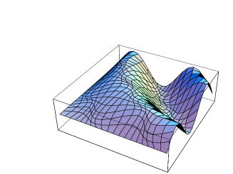
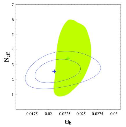
The role of relativistic species at the CMB formation, at redshifts of the order of $z\sim 1100$, is mainly to shift the matter radiation equality time, which results in both shifting the peak location in angular scale and changing the power around the first acoustic peak. This is basically due to a change in the early integrated Sachs-Wolfe effect. Several groups have studied this topics, obtaining comparable bounds on $N_{eff}$ but using different priors crotty -cuoco . For example, in our analysis cuoco , $N_{eff}=2.6^{+3.5}_{-2.0}$, using WMAP data only and weak prior on the value of the Hubble parameter, $h=0.7\pm 0.2$. The reason for such a wide range for $N_{eff}$ is ultimately due to the many unknown cosmological parameters which determine the power spectrum, and in particular to the presence of several degeneracies, i.e. the fact that different choices for some of these parameters produce the very same power spectrum. As an example if we increase both $N_{eff}$ and the amount of dark matter $\Omega_{cdm}$ we can obtain the same power spectrum provided we do not change the radiation-matter equality. This is shown in Fig.1, a plot of the bi-dimensional likelihood contours in the $N_{eff}-\Omega_{cdm}$ plane

Figure 5: Likelihood contours from WMAP data in the ${N_{eff}}$ (x-axis) - $\Omega_{cdm}h^{2}$ (y-axis) plane cuoco .

Figure 6: The 68 and 95% C.L. likelihood contours from WMAP data in the ${N_{eff}}-{\omega_{b}}$ plane.

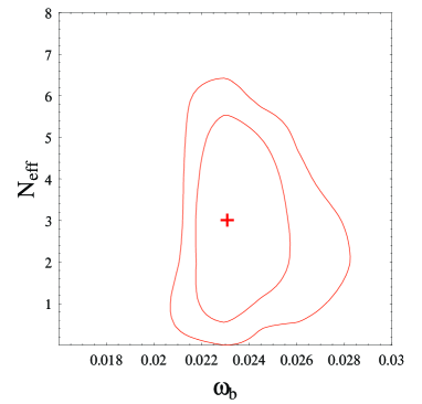
The baryon density parameter $\Omega_{b}h^{2}$ can be much more severely constrained from the power spectrum. Increasing the baryons in the plasma enhances the effective mass of the fluid and this leads to more pronounced compression peaks. By a likelihood analysis the bound obtained in cuoco is $\Omega_{b}h^{2}=0.023\pm 0.002$ ($1-\sigma$ error), fully compatible with the one quoted by the WMAP Collaboration, $\Omega_{b}h^{2}=0.022\pm 0.001$, GPMwmap . In Fig.2 we show the likelihood contours in the $N_{eff}-\Omega_{b}h^{2}$ plane. This result is extremely important. The WMAP data tell us the value of baryon density with a better accuracy than BBN, so we can test the standard scenario of light nuclei formation with basically no free parameters but the value of $N_{eff}$.

14 $\Omega_{b}h^{2}$ and $N_{eff}$ and Big Bang Nuclesynthesis

The primordial production of light nuclei, mainly ${}^{4}He$, $D$ and ${}^{7}Li$, takes place when the temperature of the electromagnetic plasma is in the range $1\div 0.01MeV$, and is strongly influenced by the two parameters $\Omega_{b}h^{2}$ and ${N_{eff}}$. Increasing the value of the baryon to photon number density enhances the fusion mechanism, so it leads to a larger eventual amount of ${}^{4}He$, the most tightly bound light nucleus (${}^{4}He$ binding energy per nucleon is of the order of $7MeV$). On the other hand, $D$ rapidly decreases with $\Omega_{b}h^{2}$, so the experimental result on this species is a very sensitive measure of baryons in the universe. The contribution of relativistic degrees of freedom to the expansion rate, parameterized by ${N_{eff}}$ affects instead the decoupling temperature of weak reaction which keep in chemical equilibrium protons and neutrons. For large temperatures in fact the ratio of their densities is given by equilibrium conditions, $n/p=\exp(-(m_{n}-m_{p})/T)$, therefore if weak interactions were efficient down to very low temperatures, much smaller than the neutron-proton mass difference, neutrons would completely disappear. We mentioned however that the rate of these processes indeed becomes smaller than the expansion rate $H$ for temperatures of the order of $T_{D}\sim 1MeV$, so that the $n/p$ ratio freezes-out at the value $n/p=\exp(-(m_{n}-m_{p})/T_{D})$. Since almost all neutrons are eventually bound in ${}^{4}He$ nuclei it is then straightforward to get for the Helium mass fraction

$$Y_{p}\equiv\frac{4n_{He}}{n_{b}}\sim 2\frac{n/p}{1+n/p}=2\frac{1}{e^{(m_{n}-m_{p})/T_{D}}+1}$$ (1)

When correcting this result for neutron spontaneous decay one gets $Y_{p}\sim 0.25$, already an excellent estimate compared with the result of detailed numerical calculations. Changing ${N_{eff}}$ affect the decoupling temperature $T_{D}$ and so the amount of primordial Helium.

An accurate analysis of BBN can be only achieved by numerically solving a set of coupled differential equations, taking into account quite a complicated network of nuclear reactions. Some of these reactions are still affected by large uncertainties, which therefore introduce an error in the theoretical prediction for, mainly, $D$ and ${}^{7}Li$ abundances. As we mentioned Helium prediction is mainly influenced by $n\leftrightarrow p$ processes, which are presently known at a high level of accuracy lopez -emmp . Quite recently a big effort has been devoted in trying to quantify the role of each nuclear reaction to the uncertainties on nuclei abundances, using either Monte Carlo krauss or linear propagation lisi techniques. The most recent analysis cuoco , burles , vangioni have benefited from the NACRE nuclear reaction catalogue nacre , as well as of very recent results, as for example the LUNA Collaboration measurement of the $D(p,\gamma)^{3}He$ luna . We report here the results obtained in cuoco for the total relative theoretical uncertainties $\sigma_{i}^{th}$ on $Y_{p}$ and $D$ and ${}^{7}Li$ number fractions $X_{i}=n_{i}/n_{b}$

$$\frac{\sigma_{D}}{X_{D}}\sim 10\%,\,\,\,\frac{\sigma_{He}}{Y_{p}}\sim 0.1\%,\,\,\,\frac{\sigma_{Li}}{X_{Li}}\sim 25\%$$ (2)

The large error on ${}^{7}Li$ is mainly due to the uncertainty on the rate for the process ${}^{4}He(^{3}He,\gamma)^{7}Be$, a process which is also of great interest for the determination of both ${}^{7}Be$ and ${}^{8}B$ neutrino fluxes from the sun. Hopefully it will be studied at low energies in the near future.

The experimental determination of primordial abundances is really a challenging task. The strategy is to identify metal poor environment, which are not been severely polluted by star contamination in their light nuclei content, and possibly to correct the observations for the effect of galactic evolution.

The ${}^{4}He$ mass fraction is determined by regression to zero metallicity of the values obtained by observing $HeII\rightarrow HeI$ recombination lines in extragalactic ionized gas. There are still quite different results (see e.g. sarkar for a review and references), a $low$ one, $Y_{p}=0.234\pm 0.003$, and a $high$ value, $Y_{p}=0.244\pm 0.002$. In the following we also use a conservative estimate, $Y_{p}=0.239\pm 0.008$.

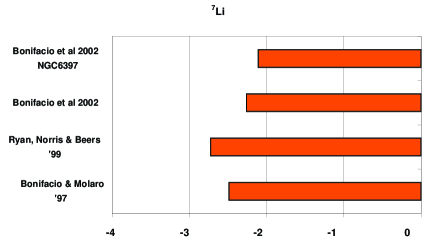
The best estimate of Primordial $D$ comes from observations of absorption lines in gas clouds in the line of sight between the earth and Quasars at very high redshift ($z\sim 2-3$), which give $X_{D}=(2.78^{+0.44}_{-0.38}){\cdot}10^{-5}$ tytler . Finally ${}^{7}Li$ is measured via observation of absorption lines in spectra of POP II halo stars, which show a saturation of ${}^{7}Li$ abundance at low metallicity (Spite plateau).

Figure 7: The pulls of QSO D measurements with respect to the theoretical prediction for ${N_{eff}}=3.04$ and ${\omega_{b}}=0.023$, in units of $\left((\sigma^{th}_{DD})^{2}+(\sigma^{exp}_{D})^{2}\right)^{1/2}$.

Figure 8: The pulls of $Y_{p}$ measurements with respect to the theoretical prediction for ${N_{eff}}=3.04$ and ${\omega_{b}}=0.023$, in units of $\left((\sigma^{th}_{44})^{2}+(\sigma^{exp}_{4})^{2}\right)^{1/2}$.

Figure 9: The pulls of $X_{7Li}$ measurements with respect to the theoretical prediction for ${N_{eff}}=3.04$ and ${\omega_{b}}=0.023$, in units of $\left((\sigma^{th}_{77})^{2}+(\sigma^{exp}_{7})^{2}\right)^{1/2}$.

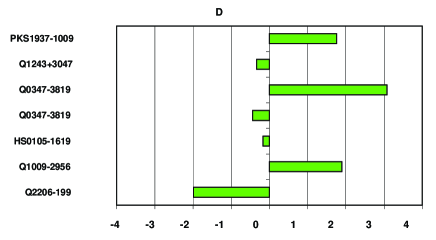
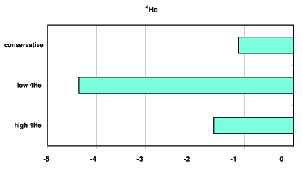
The present status of BBN, in the standard scenario, using the value of baryon density as determined by WMAP and ${N_{eff}}=3.04$ is summarized in Fig.s 3-5. Here I report the difference between the theoretical and the experimental determination, normalized to the total uncertainty, theoretical and experimental, summed in quadrature. The average of the several $D$ measurements, reported above, is indeed in very good agreement with theory. This is a very crucial result since, as we said already, $D$ is strongly influenced by $\Omega_{b}h^{2}$, which is now fixed by WMAP. In Fig. 6 I show the combined likelihood contours at $2\sigma$ in the ${N_{eff}}-\Omega_{b}h^{2}$ plane obtained when using the WMAP result $and$ $D$ measurement only (colored area) and the $D+^{4}He$ results using the conservative $Y_{p}$ shown before.

Figure 10: The 68 and $95\%$ C.L. contours for the $D+^{4}He$ likelihood function in the ${\omega_{b}}-{N_{eff}}$ plane (${\omega_{b}}=\Omega_{b}h^{2}$). We also show the result of the $CMB+D$ analysis (colored area).

It is evident that the effect of ${}^{4}He$ is to shift the values of both $\Omega_{b}h^{2}$ and ${N_{eff}}$ towards smaller values, which produces a smaller theoretical value for $Y_{p}$. Though this may be seen as a (weak) indication of the fact that a slightly lower value for ${N_{eff}}$ is preferred, I would more conservatively say that, waiting for a more clear understanding of possible systematics in $Y_{p}$ experimental determination, the standard scenario for BBN is in reasonable good shape. An open problem is however still represented by the evidence for ${}^{7}Li$ depletion, which is not fully understood (see Fig. 5). The theoretical result for $X_{Li}$ is in fact a factor 2-3 larger than the present experimental determination.

15 Neutrino-antineutrino asymmetry

While the electron-positron asymmetry density is severely constrained, of the order of $10^{-10}$ in unit of the photon density, we have no bounds at all on neutrino asymmetry from charge neutrality of the universe. Defining $\xi_{x}=\mu_{x}/T_{x}$, with $\mu_{x}$ the chemical potential for the $\nu_{x}$ species, with $x=e,\mu,\tau$, we recall that for a Fermi-Dirac distribution the particle-antiparticle asymmetry is simply related to $\xi_{x}$ (I assume here for simplicity massless neutrinos)

$$n(\nu_{x})-n(\overline{\nu}_{x})=\frac{T_{x}^{3}}{6}\left(\xi_{x}+\frac{\xi_{x}^{3}}{\pi^{2}}\right)$$ (1)

since neutrinos decoupled as hot relics starting from a chemical equilibrium condition with $e^{\pm}$, so that $\mu_{x}\equiv\mu(\nu_{x})=-\mu(\overline{\nu}_{x})$. Non vanishing values for $\xi_{x}$ affects very weakly CMB, while it is much more constrained by BBN. In fact any asymmetry in the neutrino sector contribute to the Hubble expansion rate, i.e. to ${N_{eff}}$

$${N_{eff}}\rightarrow{N_{eff}}+\sum_{x}\left[\frac{30}{7}\left(\frac{\xi_{x}}{\pi}\right)^{2}+\frac{15}{7}\left(\frac{\xi_{x}}{\pi}\right)^{4}\right]$$ (2)

In addition the asymmetry in the electron neutrino sector directly affects the $n/p$ value at the freeze-out of weak interactions, since they directly enter in the processes governing this phenomenon, namely $n+\nu_{e}\leftrightarrow p+e^{-}$, $n\leftrightarrow p+e^{-}+\overline{\nu}_{e}$ and $n+e^{+}\leftrightarrow p+\overline{\nu}_{e}$.

Figure 11: The 68 and $95\%$ C.L. likelihood contours in the $\xi_{e}-\Delta{N_{eff}}$ plane from BBN, with $\Delta{N_{eff}}={N_{eff}}-3.04$.

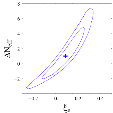
It was recently realized petcov that indeed, because of flavor oscillation, using present determination of mass differences and mixing angles from atmospheric and solar neutrinos, the three $\xi_{x}$ should be very close each other, so the bound on their (common) value $\xi$ mainly come from the fact that $\xi_{e}$ should be quite small $\xi\leq 0.1$, to give a value for the $n/p$ ratio (and so for ${}^{4}He$) in agreement with data. In Fig. 7 I show the likelihood contour obtained in the $\xi-{N_{eff}}$ plane cuoco . Though the standard BBN is preferred, there is still room for very exotic scenarios, with larger neutrino degeneracies and even very large (or very small) ${N_{eff}}$.

16 Cosmological bounds on neutrino mass scale

Despite of the fact that we presently know neutrino mass differences from oscillation effects in atmospheric and solar neutrino fluxes, there is still quite a wide range for their absolute mass scale, spanning several order of magnitude, from few $eV$ down to $10^{-2}$ $eV$. Terrestrial bounds come from Tritium decay experiments tritium , which presently give $m(\nu_{e})\leq 2.2eV$. This result will be greatly improved by next generation experiment KATRIN, which should reach a sensitivity after three years of running of the order of $0.35$ $eV$ katrin

An independent source of information will be provided by neutrinoless beta decay, which is sensitive to the effective $\nu_{e}$ mass

$$<m_{e}>=|U_{e1}|^{2}m_{1}+|U_{e2}|^{2}e^{i\phi_{2}}m_{2}+|U_{e3}|^{2}e^{i\phi_{3}}m_{3}$$ (1)

with $U_{ei}$ the electron neutrino projection onto mass eigenstates with mass $m_{i}$, and $\phi_{i}$ CP violating Majorana phases. Planned experiments CUORE cuore and GENIUS genius will have a sensitivity on this parameter of the order of $10^{-1}-10^{-2}$ $eV$.

Interestingly, quite severe constraints on neutrino masses come from cosmology. Massive neutrinos in fact contribute to the present total energy density of the Universe as $m_{\nu}n_{\nu}$ so we get

$$\Omega_{\nu}h^{2}=\frac{\sum_{x}m(\nu_{x})}{92.5\,eV}$$ (2)

which gives a generous bound when imposing $\Omega_{\nu}h^{2}<1$.

Neutrino masses however also enter in the way structures grow for gravitational instability from the initial seed likely given by adiabatic perturbations produced during the inflationary phase. In fact neutrinos free stream and tend to suppress structure formation on all scales unless they are massive. In this case they can only affect scales smaller than the Hubble horizon when they eventually become non relativistic, the ones with a corresponding wave number larger than hu

$$k_{nr}\sim 0.026\left(\frac{m_{\nu}}{1eV}\right)^{1/2}\Omega_{m}^{1/2}hMpc^{-1}$$ (3)

Several authors have recently considered this issue in details wmap2 - hann , combining WMAP data and the results of the 2dFGRS survey 2df . Actually the result also depends on the specific value of ${N_{eff}}$. A conservative value is given by $\sum_{x}m(\nu_{x})\leq 2\,eV$.

17 Acknowledgments

It is a pleasure to thank Norma Mankoc Borstnik for organizing the Portoroz meeting and for her warm hospitality. I also thank my collaborators at Naples University A. Cuoco, F. Iocco, G. Miele, O. Pisanti and P. Serpico.

*The Problem of Mass Colin D. FroggattE-mail: c.froggatt@physics.gla.ac.uk

18 Introduction

The most important unresolved problem in particle physics is the understanding of flavour and the fermion mass spectrum. The observed values of the fermion masses and mixing angles constitute the bulk of the Standard Model (SM) parameters and provide our main experimental clues to the underlying flavour dynamics. In particular the non-vanishing neutrino masses and mixings provide direct evidence for physics beyond the SM.

The charged lepton masses can be directly measured and correspond to the poles in their propagators:

$$M_{e}=0.511\ \makebox{MeV}\qquad M_{\mu}=106\ \makebox{MeV}\qquad M_{\tau}=1.78\ \makebox{GeV}$$ (4)

However the quark masses have to be extracted from the properties of hadrons and are usually quoted as running masses $m_{q}(\mu)$ evaluated at some renormalisation scale $\mu$, which are related to the propagator pole masses $M_{q}$ by

$$M_{q}=m_{q}(\mu=m_{q})\left[1+\frac{4}{3}\alpha_{3}(m_{q})\right]$$ (5)

to leading order in QCD. The light $u$, $d$ and $s$ quark masses are usually normalised to the scale $\mu=1$ GeV (or $\mu=2$ GeV for lattice measurements) and to the quark mass itself for the heavy $c$, $b$ and $t$ quarks. They are typically given pdg as follows:

$$m_{u}(1\ \makebox{GeV})=4.5\pm 1\ \makebox{MeV} m_{d}(1\ \makebox{GeV})=8\pm 2\ \makebox{MeV}$$

$$m_{c}(m_{c})=1.25\pm 0.15\ \makebox{GeV} m_{s}(1\ \makebox{GeV})=150\pm 50\ \makebox{MeV}$$

$$m_{t}(m_{t})=166\pm 5\ \makebox{GeV} m_{b}(m_{b})=4.25\pm 0.15\ \makebox{GeV}$$ (6)

However we only have an upper limit on the neutrino masses of $m_{\nu_{i}}\mathchoice{\mathrel{\vbox{\hbox{$\buildrel\displaystyle<\over{\displaystyle\sim}$}}}}{\mathrel{\vbox{\hbox{$\buildrel\textstyle<\over{\textstyle\sim}$}}}}{\mathrel{\vbox{\hbox{$\buildrel\scriptstyle<\over{\scriptstyle\sim}$}}}}{\mathrel{\vbox{\hbox{$\buildrel\scriptscriptstyle<\over{\scriptscriptstyle\sim}$}}}}1$ eV from tritium beta decay and from cosmology, and measurements of the neutrino mass squared differences:

$$\Delta m_{21}^{2}\sim 5\times 10^{-5}\makebox{eV}^{2}\qquad\Delta m_{32}^{2}\sim 3\times 10^{-3}\makebox{eV}^{2}$$ (7)

from solar and atmospheric neutrino oscillation data garcia .

The magnitudes of the quark mixing matrix $V_{CKM}$ are well measured

$$|V_{CKM}|=\begin{pmatrix}0.9734\pm 0.0008&0.2196\pm 0.0020&0.0036\pm 0.0007\cr 0.224\pm 0.016&0.996\pm 0.013&0.0412\pm 0.002\cr 0.0077\pm 0.0014&0.0397\pm 0.0033&0.9992\pm 0.0002\cr\end{pmatrix}$$ (8)

and a CP violating phase of order unity:

$$\sin^{2}\delta_{CP}\sim 1$$ (9)

can reproduce all the CP violation data. Neutrino oscillation data constrain the magnitudes of the lepton mixing matrix elements to lie in the following $3\sigma$ ranges garcia :

$$|U_{MNS}|=\begin{pmatrix}0.73-0.89&0.45-0.66&<0.24\cr 0.23-0.66&0.24-0.75&0.52-0.87\cr 0.06-0.57&0.40-0.82&0.48-0.85\cr\end{pmatrix}$$ (10)

Due to the Majorana nature of the neutrino mass matrix, there are three unknown CP violating phases $\delta$, $\alpha_{1}$ and $\alpha_{2}$ in this case garcia .

The charged fermion masses range over five orders of magnitude, whereas there seems to be a relatively mild neutrino mass hierarchy. The absolute neutrino mass scale ($m_{\nu}<1$ eV) suggests a new physics mass scale – the so-called see-saw scale $\Lambda_{seesaw}\sim 10^{15}$ GeV. The quark mixing matrix $V_{CKM}$ is also hierarchical, with small off-diagonal elements. However the elements of $U_{MNS}$ are all of the same order of magnitude except for $|U_{e3}|<0.24$, corresponding to two leptonic mixing angles being close to maximal ($\theta_{atmospheric}\simeq\pi/4$ and $\theta_{solar}\simeq\pi/6$).

We introduce the mechanism of mass protection by approximately conserved chiral charges in section 19. The top quark mass is the dominant term in the SM fermion mass matrix, so it is likely that its value will be understood dynamically before those of the other fermions. In section 20 we discuss the connection between the top quark and Higgs masses and how they can be determined from the so-called Multiple Point Principle. We present the lightest family mass generation model in section 21, which provides an ansatz for the texture of fermion mass matrices and expresses all the quark mixing angles successfully in terms of simple expressions involving quark mass ratios. The family replicated gauge group model is presented in section 22, as an example of a model whose gauge group naturally provides the mass protecting quantum numbers needed to generate the required texture for the fermion mass matrices. Finally we present a brief conclusion in section 23.

19 Fermion Mass and Mass Protection

A fermion mass term

$${\cal{L}}_{mass}=-m\overline{\psi}_{L}\psi_{R}+h.c.$$ (11)

couples together a left-handed Weyl field $\psi_{L}$ and a right-handed Weyl field $\psi_{R}$, which then satisfy the Dirac equation

$$i\gamma^{\mu}\partial_{\mu}\psi_{L}=m\psi_{R}$$ (12)

If the two Weyl fields are not charge conjugates $\psi_{L}\neq(\psi_{R})^{c}$ we have a Dirac mass term and the two fields $\psi_{L}$ and $\psi_{R}$ together correspond to a Dirac spinor. However if the two Weyl fields are charge conjugates $\psi_{L}=(\psi_{R})^{c}$ we have a Majorana mass term and the corresponding four component Majorana spinor has only two degrees of freedom. Particles carrying an exactly conserved charge, like the electron carries electric charge, must be distinct from their anti-particles and can only have Dirac masses with $\psi_{L}$ and $\psi_{R}$ having equal conserved charges. However a neutrino could be a Majorana particle.

If $\psi_{L}$ and $\psi_{R}$ have different quantum numbers, i.e. belong to inequivalent representations of a symmetry group $G$ ($G$ is then called a chiral symmetry), a Dirac mass term is forbidden in the limit of an exact $G$ symmetry and they represent two massless Weyl particles. Thus the $G$ symmetry “protects” the fermion from gaining a mass. Such a fermion can only gain a mass when $G$ is spontaneously broken.

The left-handed and right-handed top quark, $t_{L}$ and $t_{R}$, carry unequal Standard Model $SU(2)\times U(1)$ gauge charges $\textstyle Q$:

$$\mathchoice{\mbox{\boldmath$\displaystyle Q$}}{\mbox{\boldmath$\textstyle Q$}}{\mbox{\boldmath$\scriptstyle Q$}}{\mbox{\boldmath$\scriptscriptstyle Q$}}_{L}\neq\mathchoice{\mbox{\boldmath$\displaystyle Q$}}{\mbox{\boldmath$\textstyle Q$}}{\mbox{\boldmath$\scriptstyle Q$}}{\mbox{\boldmath$\scriptscriptstyle Q$}}_{R}\qquad\mathrm{(Chiral\ charges)}$$ (13)

Hence electroweak gauge invariance protects the quarks and leptons from gaining a fundamental mass term ($\overline{t}_{L}t_{R}$ is not gauge invariant). This mass protection mechanism is of course broken by the Higgs effect, when the vacuum expectation value of the Weinberg-Salam Higgs field

$$<\phi_{WS}>=\sqrt{2}v=246\ GeV$$ (14)

breaks the gauge symmetry and the SM gauge invariant Yukawa couplings $\frac{y_{i}}{\sqrt{2}}$ generate the running quark masses $m_{i}=y_{i}v=174\,y_{i}\ \makebox{GeV}$. In this way a top quark mass of the same order of magnitude as the SM Higgs field vacuum expectation value (VEV) is naturally generated (with $y_{t}$ unsuppressed). Thus the Higgs mechanism explains why the top quark mass is suppressed, relative to the fundamental (Planck, GUT…) mass scale of the physics beyond the SM, down to the scale of electroweak gauge symmetry breaking. However the further suppression of the other quark-lepton masses ($y_{b}$, $y_{c}$, $y_{s}$, $y_{u}$, $y_{d}$ $\ll$ 1) remains a mystery, which it is natural to attribute to mass protection by other approximately conserved chiral gauge charges beyond the SM, as discussed in section 22 for the family replicated gauge group model.

Fermions which are vector-like under the SM gauge group ($\mathchoice{\mbox{\boldmath$\displaystyle Q$}}{\mbox{\boldmath$\textstyle Q$}}{\mbox{\boldmath$\scriptstyle Q$}}{\mbox{\boldmath$\scriptscriptstyle Q$}}_{L}=\mathchoice{\mbox{\boldmath$\displaystyle Q$}}{\mbox{\boldmath$\textstyle Q$}}{\mbox{\boldmath$\scriptstyle Q$}}{\mbox{\boldmath$\scriptscriptstyle Q$}}_{R}$) are not mass protected and are expected to have a large mass associated with new (grand unified, string,..) physics. The Higgs particle, being a scalar, is not mass protected and a priori would also be expected to have a large mass; this is the well-known gauge hierarchy problem discussed at Portoroz by Holger Nielsen holger .

20 Top Quark and Higgs Masses from the Multiple Point Principle

Figure 12: SM bounds in the ($m_{t}$,$m_{H}$) plane for various values of $\Lambda=Q$, the scale at which new physics enters.

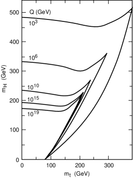
It is well-known maiani that the self-consistency of the pure SM up to some physical cut-off scale $\Lambda$ imposes constraints on the top quark and Higgs boson masses. The first constraint is the so-called triviality bound: the running Higgs coupling constant $\lambda(\mu)$ should not develop a Landau pole for $\mu<\Lambda$. The second is the vacuum stability bound: the running Higgs coupling constant $\lambda(\mu)$ should not become negative leading to the instability of the usual SM vacuum. These bounds are illustrated lindner in Fig. 12, where the combined triviality and vacuum stability bounds for the SM are shown for different values of the high energy cut-off $\Lambda$. The allowed region is the area around the origin bounded by the co-ordinate axes and the solid curve labelled by the appropriate value of $\Lambda$. The upper part of each curve corresponds to the triviality bound. The lower part of each curve coincides with the vacuum stability bound and the point in the top right hand corner, where it meets the triviality bound curve, is the infra-red quasi-fixed point for that value of $\Lambda$. Here the vacuum stability curve, for a large cut-off of order the Planck scale $\Lambda_{Planck}\simeq 10^{19}$ GeV, is important for the discussion of the values of the top quark and Higgs boson masses predicted from the Multiple Point Principle.

Figure 13: SM vacuum stability curve for $\Lambda=10^{19}$ GeV and $\alpha_{s}=0.124$ (solid line), $\alpha_{s}=0.118$ (upper dashed line), $\alpha_{s}=0.130$ (lower dashed line).

According to the Multiple Point Principle (MPP), Nature chooses coupling constant values such that a number of vacuum states have the same energy density (cosmological constant). This fine-tuning of the coupling constants is similar to that of temperature for a mixture of co-existing phases such as ice and water. We have previously argued glasgowbrioni that baby-universe like theories baby , having a mild breaking of locality and causality, may contain the underlying physical explanation of the MPP, but it really has the status of a postulated new principle. Here we apply it to the pure Standard Model fn2 , which we assume valid up close to $\Lambda_{Planck}$. So we shall postulate that the effective potential $V_{eff}(\phi)$ for the SM Higgs field $\phi$ should have a second minimum, at $<\phi>=\phi_{vac\;2}$, degenerate with the well-known first minimum at the electroweak scale $<\phi>=\phi_{vac\;1}=246$ GeV:

$$V_{eff}(\phi_{vac\;1})=V_{eff}(\phi_{vac\;2})$$ (15)

Thus we predict that our vacuum is barely stable and we just lie on the vacuum stability curve in the top quark, Higgs particle (pole) mass ($M_{t}$, $M_{H}$) plane, shown casas in Fig. 13 for a cut-off $\Lambda=10^{19}$ GeV. Furthermore we expect the second minimum to be within an order of magnitude or so of the fundamental scale, i.e. $\phi_{vac\;2}\simeq\Lambda_{Planck}$. In this way, we essentially select a particular point on the SM vacuum stability curve and hence the MPP condition predicts precise values for $M_{t}$ and $M_{H}$.

Figure 14: Plots of $\lambda$ and $g_{t}$ as functions of the scale of the Higgs field $\phi$ for degenerate vacua with the second Higgs VEV at the Planck scale $\phi_{vac\;2}=10^{19}$ GeV. We formally apply the second order SM renormalisation group equations up to a scale of $10^{25}$ GeV.

For large values of the SM Higgs field $\phi>>\phi_{vac\;1}$, the renormalisation group improved tree level effective potential is very well approximated by

$$V_{eff}(\phi)\simeq\frac{1}{8}\lambda(\mu=|\phi|)|\phi|^{4}$$

and the degeneracy condition, eq. (15), means that $\lambda(\phi_{vac\;2})$ should vanish to high accuracy. The derivative of the effective potential $V_{eff}(\phi)$ should also be zero at $\phi_{vac\;2}$, because it has a minimum there. Thus at the second minimum of the effective potential the beta function $\beta_{\lambda}$ vanishes as well:

$$\beta_{\lambda}(\mu=\phi_{vac\;2})=\lambda(\phi_{vac\;2})=0$$ (16)

which gives to leading order the relationship:

$$\frac{9}{4}g_{2}^{4}+\frac{3}{2}g_{2}^{2}g_{1}^{2}+\frac{3}{4}g_{1}^{4}-12g_{t}^{4}=0$$ (17)

between the top quark Yukawa coupling $g_{t}(\mu)$ and the electroweak gauge coupling constants $g_{1}(\mu)$ and $g_{2}(\mu)$ at the scale $\mu=\phi_{vac\;2}\simeq\Lambda_{Planck}$. We use the renormalisation group equations to relate the couplings at the Planck scale to their values at the electroweak scale. Figure 14 shows the running coupling constants $\lambda(\phi)$ and $g_{t}(\phi)$ as functions of $\log(\phi)$. Their values at the electroweak scale give our predicted combination of pole masses fn2 :

$$M_{t}=173\pm 5\ \mbox{GeV}\quad M_{H}=135\pm 9\ \mbox{GeV}$$ (18)

We have also considered metaMPP a slightly modified version of MPP, according to which the two vacua are approximately degenerate in such a way that they should both be physically realised over comparable amounts of space-time four volume. This modified MPP corresponds to the Higgs mass lying on the vacuum metastability curve rather than on the vacuum stability curve, giving a Higgs mass prediction of $122\pm 11$ GeV. We should presumably not really take the MPP predictions to be more accurate than to the order of magnitude of the variation between the metastability and stability bounds. However we definitely predict a light Higgs mass in this range, as seems to be in agreement with indirect estimates of the SM Higgs mass from precision data pdg .

This application of the MPP assumes the existence of the hierarchy

$$v/\Lambda_{Planck}\sim 10^{-17}.$$

Recently we have speculated itepfn that this huge scale ratio is a consequence of the existence of yet another vacuum in the SM, at the electroweak scale and degenerate with the two vacua discussed above. The two SM vacua at the electroweak scale are postulated to differ by the condensation of an S-wave bound state formed from 6 top and 6 anti-top quarks mainly due to Higgs boson exchange forces. This scenario is discussed in more detail in Holger Nielsen’s talk holger .

21 Lightest Family Mass Generation Model

Motivated by the famous Fritzsch ansatz fritzsch for the two generation quark mass matrices:

$$M_{U}=\begin{pmatrix}0&B\cr B^{\ast}&A\cr\end{pmatrix}\qquad M_{D}=\begin{pmatrix}0&B^{\prime}\cr B^{\prime\ast}&A^{\prime}\cr\end{pmatrix}$$ (19)

several ansätze have been proposed for the fermion mass matrices—for example, see rrr for a systematic analysis of symmetric quark mass matrices with texture zeros at the SUSY-GUT scale. Here I will concentrate on the lightest family mass generation model lfm . It successfully generalizes the well-known formula

$$\left|V_{us}\right|\simeq\left|\sqrt{\frac{m_{d}}{m_{s}}}-e^{i\phi}\sqrt{\frac{m_{u}}{m_{c}}}\right|$$ (20)

for the Cabibbo angle derived from the above ansatz, eq. (19), to simple working formulae for all the quark mixing angles in terms of quark mass ratios. According to this model the flavour mixing for quarks is basically determined by the mechanism responsible for generating the physical masses of the up and down quarks, $m_{u}$ and $m_{d}$ respectively. So, in the chiral symmetry limit, when $m_{u}$ and $m_{d}$ vanish, all the quark mixing angles vanish. Therefore we are led to consider an ansatz in which the diagonal mass matrix elements for the second and third generations are practically the same in the gauge (unrotated) and physical bases.

The mass matrix for the down quarks ($D$ = $d$, $s$, $b$) is taken to be hermitian with three texture zeros of the following form:

$$M_{D}=\begin{pmatrix}0&a_{D}&0\cr a_{D}^{\ast}&A_{D}&b_{D}\cr 0&b_{D}^{\ast}&B_{D}\cr\end{pmatrix}$$ (21)

where

$$B_{D}=m_{b}+\delta_{D}\qquad A_{D}=m_{s}+\delta_{D}^{\prime}\qquad|\delta_{D}|\ll m_{s}\qquad|\delta_{D}^{\prime}|\ll m_{d}$$ (22)

It is, of course, necessary to assume some hierarchy between the elements, which we take to be: $B_{D}\gg A_{D}\sim\left|b_{D}\right|\gg\left|a_{D}\right|$. The zero in the $\left(M_{D}\right)_{11}$ element corresponds to the commonly accepted conjecture that the lightest family masses appear as a direct result of flavour mixings. The zero in $\left(M_{D}\right)_{13}$ means that only minimal “nearest neighbour” interactions occur, giving a tridiagonal matrix structure. Since the trace and determinant of the hermitian matrix $M_{D}$ gives the sum and product of its eigenvalues, it follows that

$$\delta_{D}\simeq-m_{d}$$ (23)

while $\delta_{D}^{\prime}$ is vanishingly small and can be neglected in further considerations.

It may easily be shown that equations (21 - 23) are entirely equivalent to the condition that the diagonal elements ($A_{D}$, $B_{D}$) of $M_{D}$ are proportional to the modulus square of the off-diagonal elements ($a_{D}$, $b_{D}$):

$$\frac{A_{D}}{B_{D}}=\left|\frac{a_{D}}{b_{D}}\right|^{2}$$ (24)

Using the conservation of the trace, determinant and sum of principal minors of the hermitian matrix $M_{D}$ under unitary transformations, we are led to a complete determination of the moduli of all its elements, which can be expressed to high accuracy as follows:

$$\left|M_{D}\right|=\begin{pmatrix}0&\sqrt{m_{d}m_{s}}&0\cr\sqrt{m_{d}m_{s}}&m_{s}&\sqrt{m_{d}m_{b}}\cr 0&\sqrt{m_{d}m_{b}}&m_{b}-m_{d}\cr\end{pmatrix}$$ (25)

The mass matrix for the up quarks is taken to be of the following hermitian form:

$$M_{U}=\begin{pmatrix}0&0&c_{U}\cr 0&A_{U}&0\cr c_{U}^{\ast}&0&B_{U}\cr\end{pmatrix}$$ (26)

The moduli of all the elements of $M_{U}$ can also be readily determined in terms of the physical masses as follows:

$$\left|M_{U}\right|=\begin{pmatrix}0&0&\sqrt{m_{u}m_{t}}\cr 0&m_{c}&0\cr\sqrt{m_{u}m_{t}}&0&m_{t}-m_{u}\cr\end{pmatrix}$$ (27)

The CKM quark mixing matrix elements can now be readily calculated by diagonalising the mass matrices $M_{D}$ and $M_{U}$. They are given in terms of quark mass ratios as follows:

$$\left|V_{us}\right|=\sqrt{\frac{m_{d}}{m_{s}}}=0.222\pm 0.004\qquad\left|V_{us}\right|_{exp}=0.221\pm 0.003$$ (28)

$$\left|V_{cb}\right|=\sqrt{\frac{m_{d}}{m_{b}}}=0.038\pm 0.004\qquad\left|V_{cb}\right|_{exp}=0.039\pm 0.003$$ (29)

$$\left|V_{ub}\right|=\sqrt{\frac{m_{u}}{m_{t}}}=0.0036\pm 0.0006\qquad\left|V_{ub}\right|_{exp}=0.0036\pm 0.0006$$ (30)

$$\left|V_{td}\right|=\left|V_{us}V_{cb}-V_{ub}\right|=0.009\pm 0.002\qquad\left|V_{ub}\right|_{exp}=0.0077\pm 0.0014$$ (31)

As can be seen, they are in impressive agreement with the experimental values. The MNS lepton mixing matrix can also be fitted, if the texture of eq. (21) is extended to the Dirac and Majorana right-handed neutrino mass matrices matsuda .

The proportionality condition, eq. (24), is not so easy to generate from an underlying symmetry beyond the Standard Model, but it is possible to realise it in a local chiral $SU(3)$ family symmetry model SU3 .

22 Family Replicated Gauge Group Model

As pointed out in section 19, a natural explanation of the charged fermion mass hierarchy would be mass protection due to the existence of some approximately conserved chiral charges beyond the SM. An attractive possibility is that these chiral charges arise as a natural feature of the gauge symmetry group of the fundamental theory beyond the SM. This is the case in the family replicated gauge group model (also called the anti-grand unification model) smg3m ; fnt . The new chiral charges provide selection rules forbidding the transitions between the various left-handed and right-handed quark-lepton states, except for the top quark. In order to generate mass terms for the other fermion states, we have to introduce new Higgs fields, which break the symmetry group $G$ of the fundamental theory down to the SM group. We also need suitable intermediate fermion states to mediate the forbidden transitions, which we take to be vector-like Dirac fermions with a mass of order the fundamental scale $M_{F}$ of the theory. In this way effective SM Yukawa coupling constants are generated fn1 , which are suppressed by the appropriate product of Higgs field VEVs measured in units of $M_{F}$. We assume that all the couplings in the fundamental theory are unsuppressed, i.e. they are all naturally of order unity.

The family replicated gauge group model is based on a non-simple non-supersymmetric extension of the SM with three copies of the SM gauge group—one for each family or generation. With the inclusion of three right-handed neutrinos, the gauge group becomes $G=(SMG\times U(1)_{B-L})^{3}$, where the three copies of the SM gauge group are supplemented by an abelian $(B-L)$ (= baryon number minus lepton number) gauge group for each family. The gauge group $G$ is the largest anomaly free group, transforming the known 45 Weyl fermions plus the three right-handed neutrinos into each other unitarily, which does not unify the irreducible representations under the SM gauge group. It is supposed to be effective at energies near to the Planck scale, $M_{F}=\Lambda_{Planck}$, where the $i$’th proto-family couples to just the $i$’th group factor $SMG_{i}\times U(1)_{B_{i}-L_{i}}$. The gauge group $G$ is broken down by four Higgs fields $W$, $T$, $\rho$ and $\omega$, having VEVs about one order of magnitude lower than the Planck scale, to its diagonal subgroup:

$$(SMG\times U(1)_{B-L})^{3}\rightarrow SMG\times U(1)_{B-L}$$ (32)

The diagonal $U(1)_{B-L}$ is broken down at the see-saw scale, by another Higgs field $\phi_{SS}$, and the diagonal $SMG$ is broken down to $SU(3)\times U(1)_{em}$ by the Weinberg-Salam Higgs field $\phi_{WS}$.

Table 1: All $U(1)$ quantum charges of the Higgs fields in the $(SMG\times U(1)_{B-L})^{3}$ model.

	$y_{1}/2$	$y_{2}/2$	$y_{3}/2$	$(B-L)_{1}$	$(B-L)_{2}$	$(B-L)_{3}$
$\omega$	$\frac{1}{6}$	$-\frac{1}{6}$	$0$	$0$	$0$	$0$
$\rho$	$0$	$0$	$0$	$-\frac{1}{3}$	$\frac{1}{3}$	$0$
$W$	$0$	$-\frac{1}{2}$	$\frac{1}{2}$	$0$	$-\frac{1}{3}$	$\frac{1}{3}$
$T$	$0$	$-\frac{1}{6}$	$\frac{1}{6}$	$0$	$0$	$0$
$\phi_{\scriptscriptstyle WS}$	$0$	$\frac{2}{3}$	$-\frac{1}{6}$	$0$	$\frac{1}{3}$	$-\frac{1}{3}$
$\phi_{\scriptscriptstyle SS}$	$0$	$1$	$-1$	$0$	$2$	$0$

The $(SMG\times U(1)_{B-L})^{3}$ gauge quantum numbers of the quarks and leptons are uniquely determined by the structure of the model and they include 6 chiral abelian charges—the weak hypercharge $y_{i}/2$ and $(B-L)_{i}$ quantum number for each of the three families, $i=1,2,3$. With the choice of the abelian charges in Table 1 for the Higgs fields, it is possible to generate a good order of magnitude fit to the SM fermion masses, with VEVs of order $M_{F}/10$. In this fit, we do not attempt to guess the spectrum of superheavy fermions at the Planck scale, but simply assume a sufficiently rich spectrum to mediate all of the symmetry breaking transitions in the various mass matrix elements. Then, using the quantum numbers of Table 1, the suppression factors are readily calculated as products of Higgs field VEVs measured in Planck units for all the fermion Dirac mass matrix elements, giving for example:

$$M_{\scriptscriptstyle U}\simeq\frac{\left\langle(\phi_{\scriptscriptstyle\rm WS})^{\dagger}\right\rangle}{\sqrt{2}}\left(\!\begin{array}[]{ccc}(\omega^{\dagger})^{3}W^{\dagger}T^{2}&\omega\rho^{\dagger}W^{\dagger}T^{2}&\omega\rho^{\dagger}(W^{\dagger})^{2}T\\ (\omega^{\dagger})^{4}\rho W^{\dagger}T^{2}&W^{\dagger}T^{2}&(W^{\dagger})^{2}T\\ (\omega^{\dagger})^{4}\rho&1&W^{\dagger}T^{\dagger}\end{array}\!\right)$$ (36)

for the up quarks. Similarly the right-handed neutrino Majorana mass matrix is of order:

$$M_{R}\simeq\left\langle\phi_{\scriptscriptstyle\rm SS}\right\rangle\left(\begin{array}[]{ccc}(\rho^{\dagger})^{6}T^{6}&(\rho^{\dagger})^{3}T^{6}&(\rho^{\dagger})^{3}W^{3}(T^{\dagger})^{3}\\ (\rho^{\dagger})^{3}T^{6}&T^{6}&W^{3}(T^{\dagger})^{3}\\ (\rho^{\dagger})^{3}W^{3}(T^{\dagger})^{3}&W^{3}(T^{\dagger})^{3}&W^{6}(T^{\dagger})^{12}\end{array}\right)$$ (40)

and the effective light neutrino mass matrix can be calculated from the Dirac neutrino mass matrix $M_{N}$ and $M_{R}$ using the see-saw formula seesaw :

$$M_{\nu}=M_{N}M_{R}^{-1}M_{N}^{T}$$ (41)

In this way we obtain a good 5 parameter fit to the orders of magnitude of all the quark-lepton masses and mixing angles, as given in Table 2, actually even with the expected accuracy douglas .

Table 2: Best fit to quark-lepton mass spectrum. All masses are running masses at $1~{}\mbox{\rm GeV}$ except the top quark mass which is the pole mass.

$$\begin{array}[]{|c|c|c|}\hline\cr\hline\cr&{\rm Fitted}&{\rm Experimental}\\ \hline\cr m_{u}&4.4~{}\mbox{\rm MeV}&4~{}\mbox{\rm MeV}\\ m_{d}&4.3~{}\mbox{\rm MeV}&9~{}\mbox{\rm MeV}\\ m_{e}&1.6~{}\mbox{\rm MeV}&0.5~{}\mbox{\rm MeV}\\ m_{c}&0.64~{}\mbox{\rm GeV}&1.4~{}\mbox{\rm GeV}\\ m_{s}&295~{}\mbox{\rm MeV}&200~{}\mbox{\rm MeV}\\ m_{\mu}&111~{}\mbox{\rm MeV}&105~{}\mbox{\rm MeV}\\ M_{t}&202~{}\mbox{\rm GeV}&180~{}\mbox{\rm GeV}\\ m_{b}&5.7~{}\mbox{\rm GeV}&6.3~{}\mbox{\rm GeV}\\ m_{\tau}&1.46~{}\mbox{\rm GeV}&1.78~{}\mbox{\rm GeV}\\ V_{us}&0.11&0.22\\ V_{cb}&0.026&0.041\\ V_{ub}&0.0027&0.0035\\ \hline\cr\Delta m^{2}_{\odot}&9.0\times 10^{-5}~{}\mbox{\rm eV}^{2}&5.0\times 10^{-5}~{}\mbox{\rm eV}^{2}\\ \Delta m^{2}_{\rm atm}&1.7\times 10^{-3}~{}\mbox{\rm eV}^{2}&2.5\times 10^{-3}~{}\mbox{\rm eV}^{2}\\ \tan^{2}\theta_{\odot}&0.26&0.34\\ \tan^{2}\theta_{\rm atm}&0.65&1.0\\ \tan^{2}\theta_{\rm chooz}&2.9\times 10^{-2}&\raisebox{-2.58334pt}{${\textstyle\stackrel{{\scriptstyle<}}{{\sim}}}$}~{}2.6\times 10^{-2}\\ \hline\cr\hline\cr\end{array}$$

23 Conclusion

The hierarchical structure of the quark-lepton spectrum was emphasized and interpreted as due to the existence of a mass protection mechanism, controlled by approximately conserved chiral flavour quantum numbers beyond the SM. The family replicated gauge group model assigns a unique set of anomaly free gauge charges to the quarks and leptons. With an appropriate choice of quantum numbers for the Higgs fields, these chiral charges naturally generate a realistic set of quark-lepton masses and mixing angles. The top quark dominates the fermion mass matrices and we showed how the Multiple Point Principle can be used to predict the top quark and SM Higgs boson masses. We also discussed the lightest family mass generation model, which gives simple and compact formulae for all the CKM mixing angles in terms of the quark masses.

*How to Approach Quantum Gravity – Background Independence in $1+1$ Dimensions Daniel Grumiller and Wolfgang Kummer

24 Introduction

It has been realized for some time that a merging of quantum theory with Einstein’s theory of general relativity (GR) is necessitated by consistency arguments. In Gedankenexperimenten the interaction of a classical gravitational wave with a quantum system inevitably leads to contradictions Eppley:1977 . Arguments of this type are important because no relevant experimental data are available – we are very far from the quantum gravity analogue of the Balmer series.

On the other hand, when a quantum theory (QT) of gravity is developed along usual lines, one is confronted with a fundamental problem, from which many other (secondary) difficulties can be traced. The crucial difference to quantum field theory (QFT) in flat space is the fact that the variables of gravity exhibit a dual role, they are fields living on a manifold which is determined by themselves, “stage” and “actors” coincide. But there exist also numerous other problems: the time variable, an object with special properties already in QT, in GR appears on an equal footing with the space coordinates (“problem of time” which manifests itself in many disguises); the information paradox Banks:1995ph ; perturbative non-renormalizability 'tHooft:1974bx etc.

In section 25 we discuss some key-points regarding the definition of physical observables in QFT and the ensuing ones in quantum gravity (QGR). Then we critically mention some “old” and “new” approaches to QGR (section 26) from a strictly quantum field theorist’s point of view. Finally we give some highlights on the “Vienna approach” to 2d dilaton quantum gravity with matter, including a new result (within that approach) on entropy corrections which is in agreement with the one found in literature (section 27). In that area which contains also models with physical relevance (e.g. spherically reduced gravity) the application of just the usual concepts of (even nonpertubative!) QFT lead to very interesting consequences Grumiller:2002nm which allow physical interpretations in terms of “solid” traditional QFT observables.

25 Observables

25.1 Cartan variables in GR

Physical observables in the sense used here are certain functionals of the field variables which are directly accessible to experimental measurements.

The metric $g$ in GR can be considered as a “derived” field variable

$$g=e^{a}\otimes e^{b}\eta_{ab},$$ (42)

because it is the direct product of the dual basis one forms $e^{a}=e_{\mu}^{a}\,dx^{\mu}$ contracted with the flat local Lorentz metric $\eta_{ab}$ which is used to raise and lower “flat indices” denoted by Latin letters ($\eta={\rm diag}(1,-1,-1,-1,....),\,\,x^{\mu}=\left\{x^{0},x^{i}\right\}$). Local Lorentz invariance leads to the “covariant derivative” $D^{a}{}_{b}=\delta_{b}^{a}d+\omega^{a}{}_{b}$ with a spin connection 1-form $\omega^{a}{}_{b}$ as a gauge field. Its antisymmetry $\omega^{ab}=-\omega^{ba}$ implies metricity. Thanks to the Bianchi identities all covariant tensors relevant for constructing actions in even dimensions can be expressed in terms of $e^{a}$, the curvature 2-form $R^{ab}=(D\omega)^{ab}$ and the torsion 2-form $T^{a}=(De)^{a}$. For nonvanishing torsion the affine connection $\Gamma_{\mu\nu}$$\,{}^{\rho}=E_{a}^{\rho}\,\left(D_{\mu}e\right)_{\nu}^{a}$, expressed in terms of components $e_{\mu}^{a}$ and of its inverse $E_{a}^{\rho}$, besides the usual Christoffel symbols also contains a contorsion term in $\Gamma_{\left(\mu\nu\right)}\,^{\rho}$, whereas $\Gamma_{\left[\mu\nu\right]}\,^{\rho}$ are the components of torsion. Einstein gravity in d=4 dimensions postulates vanishing torsion $T^{a}=0$ so that $\omega=\omega(e)$. This theory can be derived from the Hilbert action ($G_{N}$ is Newton’s constant; dS space results for nonvanishing cosmological constant $\Lambda$ from the replacement $R^{ab}\rightarrow R^{ab}-\frac{4}{3}\Lambda e^{a}\wedge e^{b}$)

$$L_{\left(H\right)}=\frac{1}{16\pi G_{n}}\int_{\mathcal{M}_{4}}\,R^{ab}\wedge e^{c}\wedge e^{d}\epsilon_{abcd}+L_{\left({\rm matter}\right)}.$$ (43)

Because of the “Palatini mystery”, independent variation of $\delta\omega$ yields $T^{a}=0,$ whereas $\delta e$ produces the Einstein equations.

Instead of working with the metric (42) the “new” approaches Sen:1982qb are based upon a gauge field related to $\omega^{ab}$

$$A^{ab}=\frac{1}{2}\left(\omega^{ab}-\frac{\gamma}{2}\epsilon^{ab}{}_{cd}\,\omega^{cd}\right).$$ (44)

The Barbero-Immirzi parameter $\gamma$ Barbero:1995ap is an arbitrary constant. The extension to complex gravity $\left(\gamma=i\right)$ makes $A^{a}$ a self-adjoint field and transforms the Einstein theory into the one of an $SU\left(2\right)$ gauge field

$$A_{i}^{\underline{a}}=\epsilon^{0\,\underline{a}}\,_{\underline{b}\,\underline{c}}\,A_{i}^{\,\underline{b}\,\underline{c}},$$ (45)

where the index $\underline{a}=1,2,3.$ This formulation is the basis of loop quantum gravity and spin foam models (see below).

25.2 Observables in classical GR

The exploration of the global properties of a certain solution of (43), its singularity structure etc., is only possible by means of the introduction of an additional test field, most simply a test particle with action

$$L_{\left({\rm test}\right)} = -m_{0}\int\left|ds\right|,$$

$$ds^{2} = g_{\mu\nu}\left(x\left(\tau\right)\right)\frac{dx}{d\tau}^{\mu}\frac{\,dx\,^{\nu}}{d\tau},$$ (46)

which is another way to incorporate Einstein’s old proposal Einstein:1916vd of a “net of geodesics”. The path $x^{\mu}\left(\tau\right)$ is parameterized by the affine parameter $\tau$ (actually only timelike or lightlike $ds^{2}\geq 0$ describes the paths of a physical particle).

It is not appreciated always that the global properties of a manifold are defined in terms of a specific device like (46). Whereas the usual geodesics derived from (46) depend on $g_{\mu\nu}$ through the Christoffel symbols only, e.g. in the case of torsion also the contorsion may contribute (“autoparallels”) in the affine connection; spinning particles “feel” the gravimagnetic effect etc. As a consequence, when a field dependent transformation of the gravity variables is performed (e.g. a conformal transformation from a “Jordan frame” to an “Einstein frame” in Jordan-Brans-Dicke Fierz:1956 theory) the action of the device must be transformed in the same way.

25.3 Observables in QFT

In flat QFT one starts from a Schrödinger equation, dependent on field operators and, proceeding through Hamiltonian quantization to the path integral, the experimentally accessible observables are the elements of the S-matrix, or quantities expressible by those. It should be recalled that the properly defined renormalized S-matrix element obtains by amputation of external propagators in the related Green function, multiplication with polarizations and with a square root of the wave function renormalization constant, taking the mass-shell limit.

In gauge theories one encounters the additional problem of gauge-dependence, i.e. the dependence on some gauge parameter $\beta$ introduced by generic gauge fixing. Clearly the S-matrix elements must be and indeed are Kummer:2001ip independent of $\beta$. But other objects, in particular matrix-elements of gauge invariant operators $\mathcal{O}_{A}$, depend on $\beta$. In addition, under renormalization they mix with operators $\tilde{\mathcal{O}}_{\tilde{A}}$ of the same “twist” (dimension minus spin) which depend on Faddeev-Popov ghosts Dixon:1974ss and are not gauge-invariant:

$$\mathcal{O}_{A}^{\left(ren\right)}=Z_{AB}\mathcal{O}_{B}+Z_{A\tilde{B}}\tilde{\mathcal{O}}_{\tilde{B}}$$

$$\tilde{\mathcal{O}}_{\tilde{A}}^{\left(ren\right)}=\phantom{Z_{AB}\mathcal{O}_{B}+\ }Z_{\tilde{A}\tilde{B}}\tilde{\mathcal{O}}_{\tilde{B}}$$ (47)

The contribution of such operators to the S-matrix element (sic!) of e.g. the scaling limit for deep inelastic scattering Friedman:1991 of leptons on protons Gross:1973ju occurs only through the anomalous dimensions ($\propto\partial Z_{AB}/\partial\Lambda$ for a regularisation cut-off $\Lambda$). And those objects, also thanks to the triangular form of (47), are gauge-independent!

In flat QFT, as well as in QGR, the (gauge invariant) “Wilson loop”

$$W_{\left(\mathcal{C}\right)}={\rm Tr}\,P\exp{\big{(}i\oint\limits_{\mathcal{C}}A_{\mu\,dx^{\mu}}\big{)}},$$ (48)

parameterized by a path ordered closed curve $\mathcal{C},$ often is assumed to play an important role. In covariant gauges it is multiplicatively renormalizable with the renormalization constant depending on the length of $\mathcal{C}$, the UV cut-off and eventual cusp-angles in $\mathcal{C}$ Polyakov:1980ca . Still the relation to experimentally observable quantities (should one simply drop the renormalization constant or proceed Kummer:2001ip as for an S-matrix?) is unclear. Worse, for lightlike axial gauges $\left(nA\right)=0$ $\left(n^{2}=0\right)$ multiplicative renormalization is not applicable Andrasi:1999hu . Then, only for a matrix element of (48) between “on-shell gluons”, this type of renormalization is restored. Still the renormalization constant is different from covariant gauge, except for the anomalous dimension derived from it (cf. precisely that feature of operators in deep inelastic scattering).

26 Approaches to QGR

“Old” QGR worked with a separation of the two aspects of gravity variables by the decomposition of the metric

$$g_{\mu\nu}=g_{\mu\nu}^{\left(0\right)}+h_{\mu\nu},$$ (49)

which consists of a (fixed) classical background $g_{\mu\nu}^{\left(0\right)}$ (“stage”) with small quantum fluctuations $h_{\mu\nu}$ (“actors”). The “observable” (to be tested by a classical device) would be the effective matrix $g_{\mu\nu}^{\left({\rm eff}\right)}=g_{\mu\nu}^{\left(0\right)}+<h_{\mu\nu}>.$ Starting computations from the action (43) one finds that an ever increasing number of counter-terms is necessary. They are different from the terms in the Lagrangian $\mathcal{L}=\sqrt{-g}\,R/\left(16\pi G_{N}\right)$ in (43). This is the reason why QGR is called (perturbatively) “nonrenormalizable” 'tHooft:1974bx . Still, at energies E $\ll\left(G_{N}\right)^{-1/2}$, i.e. much below the Planck mass scale $m_{\rm Pl}\propto\left(G_{N}\right)^{-1/2}$, such calculations can be meaningful in the sense of an “effective low energy field theory” Donoghue:1994dn , irrespective of the fact that (perhaps by embedding gravity into string theory) by inclusion of further fields at higher energy scales (Planck scale), QGR may become renormalizable. Of course, such an approach even when it is modified by iterative inclusion of $<h_{\mu\nu}>$ into $g_{\mu\nu}^{\left(0\right)}$ etc. – which is technically quite hopeless – completely misses inherent background independent effects, i.e. effects when $g_{\mu\nu}^{\left(0\right)}=0$.

One could think also of applying nonperturbative methods developed in numerical lattice calculations for QCD. However, there are problems to define the Euclidean path integral for that, because the Euclidean action is not bounded from below (as it is the case in QCD) Gibbons:1994cg .

The quantization of gravity which – at least in principle – avoids background dependence is based upon the ADM approach to the Dirac quantization of the Hamiltonian Arnowitt:1962 . Space-time is foliated by a sequence of three dimensional space-like manifolds $\sum_{3}$ upon which the variables $g_{ij}=q_{ij}$ and associated canonical momenta $\pi_{ij}$ live. The constraints associated to the further variables lapse $\left(N_{0}\right)$ and shift $\left(N_{i}\right)$ in the Hamiltonian density

$$\mathcal{H}=N_{0}\,H^{0}\left(q,\pi\right)+N_{i}\,H^{i}\left(q,\pi\right)$$ (50)

are primary ones. The Poisson brackets of the secondary constraints $H^{\mu}$ closes. $H^{i}$ generates diffeomorphisms on $\sum_{3}$. In the quantum version of (50) the solutions of the Wheeler-deWitt equation involving the Hamiltonian constraint

$$\int\limits_{\sum_{3}}\,H^{0}\,\left(q,\,\frac{\delta}{i\delta q}\right)\mid\psi>=0$$ (51)

formally would correspond to a nonperturbative QGR. Apart from the fact that it is extremely difficult to find a general solution to (51) there are several basic problems with a quantum theory based upon that equation (e.g. no Hilbert space $\mid\psi>$ can be constructed, no preferred time foliation exists with ensuing inequivalent quantum evolutions Torre:1998eq , problems with usual “quantum causality” exist, the “axiom” that fields should commute at space like distances does not hold etc.). A restriction to a finite number of degrees of freedom (“mini superspace”) Dewitt:1967yk or infinite number of degrees of freedom (but still less than the original theory – so-called “midi superspace”) Kuchar:1971xm has been found to miss essential features.

As all physical states $\mid\psi>$ must be annihilated by the constraints $H^{\mu}$, a naive Schrödinger equation involving the Hamiltonian constraint $H^{0}$,

$$i\hbar\frac{\partial\mid\psi>}{\partial t}=H^{0}\mid\psi>=0,$$ (52)

cannot contain a time variable (“problem of time”). A kind of Schrödinger equation can be produced by the definition of a “time-function” $T\left(q,\pi,x\right)$, at the price of an even more complicated formalism Bergmann:1962 with quite ambiguous results – and the problem, how to connect those with “genuine” observables. All these problems are aggravated, when one tries to first eliminate constraints by solving them explicitly before quantization. In this way, clearly part of the quantum fluctuations are eliminated from the start. As a consequence different quantum theories, constructed in this way, are not equivalent.

The “new” gravities (loop quantum gravity, spin foam models) reformulate the quantum theory of space-time by the introduction of novel variables, based upon the concept of Wilson loops (48) applied to the gauge-field (45). The operator

$$U\left(s_{1},s_{2}\right)={\rm Tr}\,P\,\exp{\left(i\int\limits_{s_{1}}^{s_{2}}ds\frac{dx^{i}}{ds}\,A_{i}\right)}$$ (53)

defines a holonomy. It is generalized by inserting further invariant operators at intermediate points between $s_{1}$ and $s_{2}$ . From such holonomies a spin network can be created which represents spacetime (in the path integral it is dubbed “spin foam”).

These approaches claim several successes Carlip:2001wq . Introducing as a basis diffeomorphism equivalence classes of “labeled graphs” a finite Hilbert space can be constructed and some solutions of the Wheeler-deWitt equation (51) have been obtained. The methods introduce a “natural” coarse graining of space-time which implies a $UV$ cutoff. “Small” gravity around certain states leads in those cases to corresponding linearized Einstein gravity.

However, despite of very active research in this field a number of very serious open questions persists: The Hamiltonian constructed from spin networks does not lead to massless excitations (gravitons) in the classical limit. The Barbero-Immirzi parameter $\gamma$ has to be fixed by the requirement of a “correct” Bekenstein-Hawking entropy for the Black Hole. The most severe problem, however, is the one of observables. By some researchers in this field it has been claimed that by “proper gauge fixing” (!) area and volume can be obtained as quantized “observables”, which is a contradiction in itself from the point of view of QFT. We must emphasize too that also in an inherently $UV$ regularized theory (finite) renormalization remains an issue to be dealt with properly. Also the fate of S-matrix elements, which play such a central role as the proper observables in QFT, is completely unclear in these setups.

Embedding QGR into (super-)string theory Polchinski:1998rq does not remove the key problems related to the dual role of the metric. Gravity may well be a string excitation in a string/brane world of 10-11 dimensions, possibly a finite theory of everything. Nevertheless, at low energies Einstein gravity (eventually plus an antisymmetric $B$-field) remains the theory for which computations must be performed. Unfortunately, the proper choice (let alone the derivation) of a string vacuum in our d=4 space-time is an unsolved problem.

Many other approaches exist, including noncommutative geometry, twistors, causal sets, 3d approaches, dynamical triangulations, Regge calculus etc., each of which has certain attractive features and difficulties (cf. e.g. Carlip:2001wq and refs. therein).

To us all these “new” approaches appear as – very ingenious – attempts to bypass the technical problems of directly applying standard QFT to gravity – without a comprehensive solution of the main problems of QGR being in sight. Thus the main points of a “minimal” QFT for gravity should be based upon “proven concepts” of QFT with a point of departure characterizing QGR as follows:

• QGR is an “effective” low energy theory and therefore need not be renormalizable to all orders.

• QGR is based upon classical Einstein (-dS) gravity with usual variables (metric or Cartan variables).

• At least the quantization of geometry must be performed in a background independent (nonperturbative) way.

• Absolutely “safe” quantum observables are only the S-matrix elements of QFT ${<f\mid S\mid i>}$, where initial state ${\mid i>}$ and final state ${<f\mid}$ are defined only when those states are realized as Fock states of particles in a (at least approximate) flat space environment. In certain cases it is permissible to employ a semi-classical approach: expectation values of quantum corrections may be added to classical geometric variables, and a classical computation is then based on the effective variables, obtained in this way.

Clearly item (d) by construction excludes any application to quantum cosmology, where $\mid i>$ would be the (probably nonexistent) infinite past before the Big Bang.

Obviously the most difficult issue is (c). We describe in the following section how gravity models in d=2 (e.g. spherically reduced gravity) permit a solution of just that crucial point, leading to novel results.

27 “Minimal” QGR in 1+1 dimensions

27.1 Classical theory: first order formulation

In the 1990s the interest in dilaton gravity in d=2 was rekindled by results from string theory Mandal:1991tz , but it existed as a field on its own more or less since the 1980s Barbashov:1979 . For a review on dilaton gravity ref. Grumiller:2002nm may be consulted. For sake of self-containment the study of dilaton gravity will be motivated briefly from a purely geometrical point of view.

The notation of ref. Grumiller:2002nm is used: $e^{a}$ is the zweibein one-form, $\epsilon=e^{+}\wedge e^{-}$ is the volume two-form. The one-form $\omega$ represents the spin-connection $\omega^{a}{}_{b}=\varepsilon^{a}{}_{b}\omega$ with the totally antisymmetric Levi-Civitá symbol $\varepsilon_{ab}$ ($\varepsilon_{01}=+1$). With the flat metric $\eta_{ab}$ in light-cone coordinates ($\eta_{+-}=1=\eta_{-+}$, $\eta_{++}=0=\eta_{--}$) the torsion 2-form reads $T^{\pm}=(d\pm\omega)\wedge e^{\pm}$. The curvature 2-form $R^{a}{}_{b}$ can be presented by the 2-form $R$ defined by $R^{a}{}_{b}=\varepsilon^{a}{}_{b}R$, $R=d\wedge\omega$. Signs and factors of the Hodge-$\ast$ operation are defined by $\ast\epsilon=1$.

Since the Hilbert action $\int_{\mathcal{M}_{2}}R\propto(1-g)$ yields just the Euler number for a surface with genus $g$ one has to generalize it appropriately. The simplest idea is to introduce a Lagrange multiplier for curvature, $X$, also known as “dilaton field”, and an arbitrary potential thereof, $V(X)$, in the action $\int_{\mathcal{M}_{2}}\left(XR+\epsilon V(X)\right)$. In particular, for $V\propto X$ the Jackiw-Teitelboim model emerges Barbashov:1979 . Having introduced curvature it is natural to consider torsion as well. By analogy the first order gravity action Ikeda:1993aj

$$L^{(1)}=\int_{\mathcal{M}_{2}}\left(X_{a}T^{a}+XR+\epsilon\mathcal{V}(X^{a}X_{a},X)\right)$$ (54)

can be motivated where $X_{a}$ are the Lagrange multipliers for torsion. It encompasses essentially all known dilaton theories in 2d, also known as Generalized Dilaton Theories (GDT). Spherically reduced gravity (SRG) from d=4 corresponds to $\mathcal{V}=-X^{+}X^{-}/(2X)-{\rm const}$.

Without matter there are no physical propagating degrees of freedom, which is advantageous mathematically but not very attractive from a physical point of view. Thus, in order to describe scattering processes matter has to be added. The simplest way is to consider a massless Klein-Gordon field $\phi$,

$$L^{(m)}=\frac{1}{2}\;\int_{\mathcal{M}_{2}}\;F(X)\,d\phi\wedge\ast d\phi\,,$$ (55)

with a coupling function $F(X)$ depending on the dilaton (for dimensionally reduced theories typically $F\propto X$ holds).

27.2 Quantum theory: Virtual Black Holes

It turned out that even in the presence of matter an exact path integration of all geometric quantities is possible for all GDTs, proceeding along well established paths of QFT Kummer:1992rt .

The effective theory obtained in this way solely depends on the matter fields in which it is nonlocal and non-polynomial. Already at the level of the (nonlocal) vertices of matter fields, to be used in a systematic perturbative expansion in terms of Newton’s constant, a highly nontrivial and physically intriguing phenomenon can be observed, namely the so-called “virtual black hole” (VBH). This notion originally has been introduced by S. Hawking Hawking:1996ag , but in our recent approach the VBH for SRG emerges naturally in Minkowski signature space-time, without the necessity of additional ad hoc assumptions.

For non-minimally coupled scalars the lowest order S-matrix indeed exhibited interesting features: forward scattering poles, monomial scaling with energy, CPT invariance, and pseudo-self-similarity in its kinematic sector Grumiller:2000ah .

Figure 15: CP diagram of the VBH

It was possible to reconstruct geometry self-consistently from a (perturbative or, if available, exact) solution of the effective theory. For the simplest case of four-point tree-graph scattering the corresponding Carter-Penrose (CP) diagram is presented in Fig. 15. It is non-local in the sense that it depends not only on one set of coordinates but on two. This was a consequence of integrating out geometry non-perturbatively. For each choice of $y$ (one of the two sets of coordinates) it is possible to draw an ordinary CP-diagram. The non-trivial part of our effective geometry (i.e. the VBH) is concentrated on the light-like cut. For SRG the ensuing line-element has Sachs-Bondi form

$$(ds)^{2}=2drdu+\left(1-\frac{2m(u,r)}{r}-a(u,r)r+d(u,r)\right)(du)^{2}\,,$$ (56)

with $m$, $a$ and $d$ being localized on the cut $u=u_{0}$ with compact support $r<r_{0}$. These quantities depend on the second set of coordinates $u_{0}$, $r_{0}$.

One should not take the effective geometry at face value – this would be like over-interpreting the role of virtual particles in a loop diagram. It is a nonlocal entity and one still has to “sum” (read: integrate) over all possible geometries of this type in order to obtain the nonlocal vertices and the scattering amplitude. Nonetheless, the simplicity of this geometry and the fact that all possible configurations are summed over are nice features of this picture. Moreover, all VBH geometries coincide asymptotically and differ only very little from each other in the asymptotic region. This observation allows for the following interpretation: the boundaries of the diagram, $\mathcal{I}^{\pm}$ and $i^{0}$, behave in a classical way (thus enabling one to construct an ordinary Fock space like in fixed background QFT), but the more one zooms into the geometry the less classical it becomes. The situation seems to be quite contrary to Kuchař’s proposal of geometrodynamics of BHs: while we have fixed boundary conditions for the target space coordinates (and hence a fixed ADM mass) but a “smeared geometry” (in the sense that a continuous spectrum of asymptotically equivalent VBHs contributes to the S-matrix), Kuchař encountered a “smeared mass” (obeying a Schrödinger equation) but an otherwise fixed geometry Kuchar:1994zk .

Qualitatively it is clear what has to be done in order to obtain the S-matrix: Take all possible VBHs of Fig. 15 and sum them coherently with proper weight factors and suitably attached external legs of scalar fields. This had been done quantitatively in a straightforward but rather lengthy calculation for gravitational scattering of s-waves in the framework of SRG, the result of which yielded the lowest order tree-graph S-matrix for ingoing modes with momenta $q,q^{\prime}$ and outgoing ones $k,k^{\prime}$,

$$T(q,q^{\prime};k,k^{\prime})=-\frac{i\kappa\delta\left(k+k^{\prime}-q-q^{\prime}\right)}{2(4\pi)^{4}|kk^{\prime}qq^{\prime}|^{3/2}}E^{3}\tilde{T}\,,$$ (57)

with the total energy $E=q+q^{\prime}$, $\kappa=8\pi G_{N}$,

$$\tilde{T}(q,q^{\prime};k,k^{\prime}):=\frac{1}{E^{3}}{\Bigg{[}}\Pi\ln{\frac{\Pi^{2}}{E^{6}}}+\frac{1}{\Pi}\sum_{p\in\left\{k,k^{\prime},q,q^{\prime}\right\}}$$

$$p^{2}\ln{\frac{p^{2}}{E^{2}}}{\Bigg{(}}3kk^{\prime}qq^{\prime}-\frac{1}{2}\sum_{r\neq p}\sum_{s\neq r,p}\left(r^{2}s^{2}\right){\Bigg{)}}{\Bigg{]}}\,,$$ (58)

and the momentum transfer function $\Pi=(k+k^{\prime})(k-q)(k^{\prime}-q)$. The interesting part of the scattering amplitude is encoded in the scale independent factor $\tilde{T}$. The forward scattering poles occurring for $\Pi=0$ should be noted.

It is possible to generalize the VBH phenomenon to arbitrary GDTs with matter as well as most of its properties (for instance, the CP-diagram, CPT invariance and the role played in the S-matrix) Grumiller:2002dm .

27.3 New results and outlook

Recently quantum corrections to the specific heat of the dilaton BH have been calculated by applying the quantization method discussed above Grumiller:2003mc . The result is $C_{s}:=dM/dT=96\pi^{2}M^{2}/\lambda^{2}$, where $\lambda$ is the scale parameter of the theory. Thus, in that particular case quantum corrections lead to a stabilization of the system. The mass of the BH is found to be decreasing according to

$$M(u)\approx M_{0}-\frac{\pi}{6}(T_{H}^{0})^{2}(u-u_{0})-\frac{\lambda}{24\pi}\ln{\frac{M(u)}{M_{0}}}+{\mathcal{O}}\left(\frac{\lambda}{M(u)}\right)\,.$$ (59)

The first term is the ADM mass, the second term corresponds to a linear decrease due to the (in leading order) constant Hawking flux and the third term provides the first nontrivial correction.

Applying simple thermodynamical methods ($dS=C_{s}dT/T$) and exploiting the quantum corrected mass/temperature relation $T/T_{0}=1-\lambda/(48\pi M)$ it is possible to calculate also entropy corrections:

$$S=S_{0}-\frac{1}{24}\ln{S_{0}}+{\mathcal{O}}(1)\,,\quad S_{0}:=\frac{2\pi M}{\lambda}=\left.2\pi X\right|_{\rm horizon}$$ (60)

The logarithmic behavior is in qualitative agreement with the one found in the literature by various methods Mann:1998hm ; the prefactor $1/24$ coincides with Zaslavskii:1996dg .

An extension of the results obtained in the first order formulation to dilaton supergravity is straightforward in principle but somewhat tedious in detail. It permitted, among other results, to obtain for the first time a full solution of dilaton supergravity Bergamin:2003am .

All these exciting applications indicate that the strict application of standard QFT concepts to gravity (at least in d=2 or in models dimensionally reduced to d=2) shows great promise.

*Hidden Spacetime Symmetries and Generalized Holonomy in M-theoryMCTP-03-11 and hep-th/0303140^, Research supported in part by DOE Grant DE-FG02-95ER40899. Michael J. Duffmduff@umich.edu and James T. Liujimliu@umich.edu

28 Introduction

M-theory not only provides a non-perturbative unification of the five consistent superstring theories, but also embraces earlier work on supermembranes and eleven-dimensional supergravity World . It is regarded by many as the dreamed-of final theory and has accordingly received an enormous amount of attention. It is curious, therefore, that two of the most basic questions of M-theory have until now remained unanswered:

i) What are the symmetries of M-theory?

ii) How many supersymmetries can vacua of M-theory preserve?

The first purpose of this paper is to argue that M-theory possesses previously unidentified hidden spacetime (timelike and null) symmetries in addition to the well-known hidden internal (spacelike) symmetries. These take the form of generalized structure groups ${\cal G}$ that replace the Lorentz group ${\rm SO}(10,1)$.

The second purpose is to argue that the number of supersymmetries preserved by an M-theory vacuum is given by the number of singlets appearing in the decomposition of the 32-dimensional representation of ${\cal G}$ under ${\cal G}\supset{\cal H}$ where ${\cal H}$ are generalized holonomy groups.

The equations of M-theory display the maximum number of supersymmetries $N$=32, and so $n$, the number of supersymmetries preserved by a particular vacuum, must be some integer between 0 and 32. But are some values of $n$ forbidden and, if so, which ones? For quite some time it was widely believed that, aside from the maximal $n=32$, $n$ is restricted to $0\leq n\leq 16$ with $n=16$ being realized by the fundamental BPS objects of M-theory: the M2-brane, the M5-brane, the M-wave and the M-monopole. The subsequent discovery of intersecting brane configurations with $n=0$, 1, 2, 3, 4, 5, 6, 8, 16 lent credence to this argument. In Gauntletthull1 , on the other hand, it was shown that all values $0\leq n\leq 32$ are allowed by the M-theory algebra Townsend , and examples of vacua with $16<n<32$ have indeed since been found. Following Duffstelle and MDDuff , we here put forward a generalized holonomy conjecture according to which the answer lies somewhere in between. Evidence in favor of this conjecture includes the observations that there are no known counterexamples and that a previously undiscovered example predicted in MDDuff , namely $n$=14, has recently been found Harmark .

As we shall see, these conjectures are based on a group-theoretical argument which applies to the fully-fledged M-theory. To get the ball rolling, however, we begin with the low energy limit of M-theory, namely $D=11$ supergravity. The unique $D=11$ supermultiplet is comprised of a graviton $g_{MN}$, a gravitino $\Psi_{M}$ and $3$-form gauge field $A_{MNP}$, where $M=0,1,\ldots 10$, with $44$, $128$ and $84$ physical degrees of freedom, respectively. In section 29, we conjecture that the supergravity equations of motion for this set of fields admit hidden timelike and null symmetries (in addition to previously demonstrated hidden spacelike ones). Then in section 30 we propose that, so long as the $D=11$ Killing spinor equation has such hidden symmetries, we may enlarge the tangent space group into a generalized structure group. This allows us to analyze the number of supersymmetries based on a generalized holonomy conjecture. Partial justification for this conjecture is presented in section 31 in the context of a dimensionally reduced theory. In section 32 we discuss some consequences of generalized holonomy for classifying supersymmetric vacua, and finally conclude in section 33.

29 Hidden spacetime symmetries of D=11 supergravity

Long ago, Cremmer and Julia Cremmerjulia pointed out that, when dimensionally reduced to $d$ dimensions, $D=11$ supergravity exhibits hidden symmetries. For example ${\rm E}_{7}(global)\times{\rm SU}(8)(local)$ when $d=4$ and ${\rm E}_{8}(global)\times{\rm SO}(16)(local)$ when $d=3$. The question was then posed Fradkin : do these symmetries appear magically only after dimensional reduction, or were they already present in the full uncompactified and untruncated $D=11$ theory? The question was answered by de Wit and Nicolai Dewitnicolai2 ; Nicolai who made a $d/(11-d)$ split and fixed the gauge by setting to zero the off-diagonal components of the elfbein. They showed that in the resulting field equations the local symmetries are indeed already present, but the global symmetries are not. For example, after making the split ${\rm SO}(10,1)\supset{\rm SO}(3,1)\times{\rm SO}(7)$, we find the enlarged symmetry ${\rm SO}(3,1)\times{\rm SU}(8)$. There is no global ${\rm E}_{7}$ invariance (although the 70 internal components of the metric and 3-form may nevertheless be assigned to an ${\rm E}_{7}/{\rm SU}(8)$ coset). Similar results were found for other values of $d$: in each case the internal subgroup ${\rm SO}(11-d)$ gets enlarged to some compact group $G(spacelike)$ while the spacetime subgroup ${\rm SO}(d-1,1)$ remains intact. In this paper we ask instead whether there are hidden spacetime symmetries. This is a question that could have been asked long ago, but we suspect that people may have been inhibited by the Coleman-Mandula theorem which forbids combining spacetime and internal symmetries MDColeman . However, this is a statement about Poincare symmetries of the S-matrix and here we are concerned with Lorentz symmetries of the equations of motion, so there will be no conflict.

The explicit demonstration of $G(spacelike)$ invariance by de Wit and Nicolai is very involved, to say the least. However, the result is quite simple: one finds the same $G(spacelike)$ in the full uncompactified $D=11$ theory as was already found in the spacelike dimensional reduction of Cremmer and Julia. Here we content ourselves with the educated guess that the same logic applies to $G(timelike)$ and $G(null)$: they are the same as what one finds by timelike and null reduction, respectively. So we propose that, after making a $d/(11-d)$ split, the Lorentz subgroup $G={\rm SO}(d-1,1)\times{\rm SO}(11-d)$ can be enlarged to the generalized structure groups ${\cal G}={\rm SO}(d-1,1)\times G(spacelike)$, ${\cal G}={\rm ISO}(d-1)\times G(null)$ and ${\cal G}={\rm SO}(d)\times G(timelike)$ as shown in Tables 3, 4 and 5.

$d/(11-d)$	${\cal G}={\rm SO}(d-1,1)\times G(spacelike)$	$\epsilon$ representation
10/1	${\rm SO}(9,1)\times\{1\}$	$16+\overline{16}$
9/2	${\rm SO}(8,1)\times{\rm SO}(2)$	$16_{\pm 1/2}$
8/3	${\rm SO}(7,1)\times{\rm SO}(3)\times{\rm SO}(2)$	$(8_{s},2)_{1/2}+(8_{c},2)_{-1/2}$
7/4	${\rm SO}(6,1)\times{\rm SO}(5)$	$(8,4)$
6/5	${\rm SO}(5,1)\times{\rm SO}(5)\times{\rm SO}(5)$	$(4,4,1)+(\overline{4},1,4)$
5/6	${\rm SO}(4,1)\times{\rm USp}(8)$	$(4,8)$
4/7	${\rm SO}(3,1)\times{\rm SU}(8)$	$(2,1,8)+(1,2,\overline{8})$
3/8	${\rm SO}(2,1)\times{\rm SO}(16)$	$(2,16)$
2/9	${\rm SO}(1,1)\times{\rm SO}(16)\times{\rm SO}(16)$	$(16,1)_{1/2}+(1,16)_{-1/2}$
1/10	$\{1\}\times{\rm SO}(32)$	$32$

Table 3: Generalized structure groups: spacelike case. The last column denotes the representation of $\epsilon$ under ${\cal G}$.

$d/(11-d)$	${\cal G}={\rm ISO}(d-1)\times G(null)$	$\epsilon$ representation
10/1	${\rm ISO}(9)$	$16+16$
9/2	${\rm ISO}(8)\times{\mathbb{R}}$	$8_{s}+8_{s}+8_{c}+8_{c}$
8/3	${\rm ISO}(7)\times{\rm ISO}(2)\times{\mathbb{R}}$	$8_{\pm 1/2}+8_{\pm 1/2}$
7/4	${\rm ISO}(6)\times[{\rm SO}(3)\times{\rm SO}(2)]\ltimes{\mathbb{R}}^{6}_{(3,2)}$	$(4,2)_{\pm_{1}/2}+(\overline{4},2)_{\pm 1/2}$
6/5	${\rm ISO}(5)\times{\rm SO}(5)\ltimes{\mathbb{R}}^{10}_{(10)}$	$(4,4)+(4,4)$
5/6	${\rm ISO}(4)\times[{\rm SO}(5)\times{\rm SO}(5)]\ltimes{\mathbb{R}}^{16}_{(4,4)}$	$(2,1,4,1)+(2,1,1,4)$
		$+(1,2,4,1)+(1,2,1,4)$
4/7	${\rm ISO}(3)\times{\rm USp}(8)\ltimes{\mathbb{R}}^{27}_{(27)}$	$(2,8)+(2,8)$
3/8	${\rm ISO}(2)\times[{\rm SU}(8)\times{\rm U}(1)]\ltimes{\mathbb{R}}^{56}_{(28_{1/2},\overline{28}_{-1/2})}$	$(8_{1/2})_{\pm 1/2}+(\overline{8}_{-1/2})_{\pm 1/2}$
2/9	${\mathbb{R}}\times{\rm SO}(16)\ltimes{\mathbb{R}}^{120}_{(120)}$	$16+16$
1/10	$\{1\}\times[{\rm SO}(16)\times{\rm SO}(16)]\ltimes{\mathbb{R}}^{256}_{(16,16)}$	$(16,1)+(1,16)$

Table 4: Generalized structure groups: null case. The last column denotes the representation of $\epsilon$ under the maximum compact subgroup of ${\cal G}$.

$d/(11-d)$	${\cal G}={\rm SO}(d)\times G(timelike)$	$\epsilon$ representation
10/1	${\rm SO}(10)\times\{1\}$	$16+\overline{16}$
9/2	${\rm SO}(9)\times{\rm SO}(1,1)$	$16_{\pm 1/2}$
8/3	${\rm SO}(8)\times{\rm SO}(2,1)\times{\rm SO}(1,1)$	$(8_{s},2)_{1/2}+(8_{c},2)_{-1/2}$
7/4	${\rm SO}(7)\times{\rm SO}(3,2)$	$(8,4)$
6/5	${\rm SO}(6)\times{\rm SO}(5,{\mathbb{C}})$	$(4,4)+(\overline{4},\overline{4})$
5/6	${\rm SO}(5)\times{\rm USp}(4,4)$	$(4,8)$
4/7	${\rm SO}(4)\times{\rm SU}^{*}(8)$	$(2,1,8)+(1,2,\overline{8})$
3/8	${\rm SO}(3)\times{\rm SO}^{*}(16)$	$(2,16)$
2/9	${\rm SO}(2)\times{\rm SO}(16,{\mathbb{C}})$	$16_{1/2}+\overline{16}_{-1/2}$
1/10	$\{1\}\times{\rm SO}(16,16)$	$32$

Table 5: Generalized structure groups: timelike case. The last column denotes the representation of $\epsilon$ under ${\cal G}$.

Some of the noncompact groups appearing in the Tables may be unfamiliar, but a nice discussion of their properties may be found in Gilmore . For $d>2$ the groups $G(spacelike)$, $G(timelike)$ and $G(null)$ are the same as those obtained from the spacelike dimensional reductions of Cremmer and Julia Cremmerjulia , the timelike reductions of Hull and Julia Hulljulia , and the null reduction of section 30.2, respectively. For our purposes, however, their physical interpretation is very different. They are here proposed as symmetries of the full $D=11$ equations of motion; there is no compactification involved, whether toroidal or otherwise. This conjecture that these symmetries are present in the full theory and not merely in its dimensional reductions may be put to the test, however, as we shall later describe. For $d\leq 2$ it is less clear whether these generalized structure groups are actually hidden symmetries. See the caveats of section 31. The ${\rm SO}(16)\times{\rm SO}(16)$ for $d=2$ is also discussed by Nicolai Nicolai:1991tt .

30 Hidden Symmetries and Generalized Holonomy

We begin by reviewing the connection between holonomy and the number of preserved supersymmetries, $n$, of supergravity vacua. This also serves to define our notation. Subsequently, we introduce a generalized holonomy which involves the hidden symmetries conjectured in the previous section.

30.1 Riemannian Holonomy

We are interested in solutions of the bosonic field equations

$$R_{MN}=\frac{1}{12}\left(F_{MPQR}F_{N}{}^{PQR}-\frac{1}{12}g_{MN}F^{PQRS}F_{PQRS}\right)$$ (61)

and

$$d*\!F_{(4)}+{\frac{1}{2}}F_{(4)}\wedge F_{(4)}=0,$$ (62)

where $F_{(4)}=dA_{(3)}$. The supersymmetry transformation rule of the gravitino reduces in a purely bosonic background to

$$\delta\Psi_{M}={\tilde{D}}_{M}\epsilon,$$ (63)

where the parameter $\epsilon$ is a 32-component anticommuting spinor, and where

$${\tilde{D}}_{M}=D_{M}-\frac{1}{288}(\Gamma_{M}{}^{NPQR}-8\delta_{M}^{N}\Gamma^{PQR})F_{NPQR},$$ (64)

where $\Gamma^{A}$ are the $D=11$ Dirac matrices. Here $D_{M}$ is the usual Riemannian covariant derivative involving the connection $\omega_{M}$ of the usual structure group ${\rm Spin}(10,1)$, the double cover of ${\rm SO}(10,1)$,

$$D_{M}=\partial_{M}+\frac{1}{4}\omega_{M}{}^{AB}\Gamma_{AB}.$$ (65)

The number of supersymmetries preserved by an M-theory background depends on the number of covariantly constant spinors,

$${\tilde{D}}_{M}\epsilon=0,$$ (66)

called Killing spinors. It is the presence of the terms involving the 4-form $F_{(4)}$ in (64) that makes this counting difficult. So let us first examine the simpler vacua for which $F_{(4)}$ vanishes. Killing spinors then satisfy the integrability condition

$$[{D}_{M},{D}_{N}]\epsilon=\frac{1}{4}R_{MN}{}^{AB}\Gamma_{AB}\epsilon=0,$$ (67)

where $R_{MN}{}^{AB}$ is the Riemann tensor. The subgroup of ${\rm Spin}(10,1)$ generated by this linear combination of ${\rm Spin}(10,1)$ generators $\Gamma_{AB}$ corresponds to the ${\it holonomy}$ group ${H}$ of the connection $\omega_{M}$. The number of supersymmetries, $n$, is then given by the number of singlets appearing in the decomposition of the $32$ of ${\rm Spin}(10,1)$ under ${H}$. In Euclidean signature, connections satisfying (67) are automatically Ricci-flat and hence solve field equations when $F_{(4)}=0$. In Lorentzian signature, however, they need only be Ricci-null Fig so Ricci-flatness has to be imposed as an extra condition. In Euclidean signature, the holonomy groups have been classified Berger . In Lorentzian signature, much less is known but the question of which subgroups ${H}$ of ${\rm Spin}(10,1)$ leave a spinor invariant has been answered in Bryant . There are two sequences according as the vector $v_{A}=\overline{\epsilon}\,\Gamma_{A}\epsilon$ is timelike or null, as shown in Tables 6 and 7. Since $v^{2}\leq 0$, the spacelike $v_{A}$ case does not arise. The timelike $v_{A}$ case corresponds to static vacua, where ${H}\subset{\rm Spin}(10)\subset{\rm Spin}(10,1)$ while the null case to non-static vacua where ${H}\subset{\rm ISO}(9)\subset{\rm Spin}(10,1)$. It is then possible to determine the possible $n$-values Acharya:1998yv ; Acharya:1998st and one finds $n=2$, 4, 6, 8, 16, 32 for static vacua, as shown in Table 6, and $n=1$, 2, 3, 4, 8, 16, 32 for non-static vacua, as shown in Table 7.

$d/(11-d)$	$H\subset{\rm SO}(11-d)\subset{\rm Spin}(10)$	$n$
7/4	${\rm SU}(2)\cong{\rm Sp}(2)$	$16$
5/6	${\rm SU}(3)$	$8$
4/7	${\rm G}_{2}$	$4$
3/8	${\rm SU}(2)\times{\rm SU}(2)$	$8$
	${\rm Sp}(4)$	$6$
	${\rm SU}(4)$	$4$
	${\rm Spin}(7)$	$2$
1/10	${\rm SU}(2)\times{\rm SU}(3)$	$4$
	${\rm SU}(5)$	$2$

Table 6: Holonomy of static M-theory vacua with $F_{(4)}=0$ and their supersymmetries.

$d/(11-d)$	$H\subset{\rm ISO}(d-1)\times{\rm ISO}(10-d)\subset{\rm Spin}(10,1)$	$n$
10/1	${\mathbb{R}}^{9}$	$16$
6/5	${\mathbb{R}}^{5}\times({\rm SU}(2)\ltimes{\mathbb{R}}^{4})$	$8$
4/7	${\mathbb{R}}^{3}\times({\rm SU}(3)\ltimes{\mathbb{R}}^{6})$	$4$
3/8	${\mathbb{R}}^{2}\times({\rm G}_{2}\ltimes{\mathbb{R}}^{7})$	$2$
2/9	${\mathbb{R}}\times({\rm SU}(2)\ltimes{\mathbb{R}}^{4})\times({\rm SU}(2)\ltimes{\mathbb{R}}^{4})$	$4$
	${\mathbb{R}}\times({\rm Sp}(4)\ltimes{\mathbb{R}}^{8})$	$3$
	${\mathbb{R}}\times({\rm SU}(4)\ltimes{\mathbb{R}}^{8})$	$2$
	${\mathbb{R}}\times({\rm Spin}(7)\ltimes{\mathbb{R}}^{8})$	$1$

Table 7: Holonomy of non-static M-theory vacua with $F_{(4)}=0$ and their supersymmetries.

30.2 Generalized holonomy

When we want to include vacua with $F_{(4)}\neq 0$ we face the problem that the connection in (64) is no longer the spin connection to which the bulk of the mathematical literature on holonomy groups is devoted. In addition to the ${\rm Spin}(10,1)$ generators $\Gamma_{AB}$, it is apparent from (64) that there are terms involving $\Gamma_{ABC}$ and $\Gamma_{ABCDE}$. As a result, the connection takes its values in the full $D=11$ Clifford algebra. Moreover, this connection can preserve exotic fractions of supersymmetry forbidden by the Riemannian connection. For example, the M-branes at angles in Ohta include $n$=5, the 11-dimensional pp-waves in Michelson ; Cvetic:2002si ; Gauntletthull2 ; Bena include $n=18$, 20, 22, 24, 26 (and $n=28$ for Type IIB), the squashed $N(1,1)$ spaces in Page and the M5-branes in a pp-wave background in Singh include $n$=12 and the Gödel universes in Gauntlett:2002nw include $n=18$, 20, 22, 24.

However, we can attempt to quantify this in terms of generalized holonomy groups ${\cal H}\subset{\cal G}$ where ${\cal G}$ are the generalized structure groups discussed in section 29. The generalized holonomy conjecture Duffstelle ; MDDuff states that one can assign a holonomy ${\cal H}\subset{\cal G}$ to the generalized connection appearing in the supercovariant derivative (64). Here we propose that, after making a $d/(11-d)$ split, the Lorentz subgroup $G={\rm SO}(d-1,1)\times{\rm SO}(11-d)$ can be enlarged to the generalized structure groups ${\cal G}={\rm SO}(d-1,1)\times G(spacelike)$, ${\cal G}={\rm ISO}(d-1)\times G(null)$ and ${\cal G}={\rm SO}(d)\times G(timelike)$ as shown in Tables 3, 4 and 5. Note that in the right hand column of the tables we have listed the corresponding ${\cal G}$ representations under which the 32 supersymmetry parameters $\epsilon$ transform. The number of supersymmetries preserved by an M-theory vacuum is then given by the number of singlets appearing in the decomposition of these representations under ${\cal G}\supset{\cal H}$.

31 Structure groups from dimensional reduction

In this section we provide partial justification for the conjectured hidden symmetries by demonstrating their presence in the gravitino variation of the dimensionally reduced theory. In particular, we consider a spacelike dimensional reduction corresponding to a $d/(11-d)$ split. Turning on only $d$-dimensional scalars, the reduction ansatz is particularly simple

$$g^{(11)}_{MN}=\begin{pmatrix}\Delta^{-1/(d-2)}g_{\mu\nu}&0\cr 0&g_{ij}\end{pmatrix},\qquad A^{(11)}_{ijk}=\phi_{ijk},$$ (68)

where $\Delta=\det{g_{ij}}$. For $d\leq 5$, we must also consider the possibility dualizing either $F_{(4)}$ components or (for $d=3$) Kaluza-Klein vectors to scalars. We will return to such possibilities below. But for now we focus on $d\geq 6$. In this case, a standard dimensional reduction of the $D=11$ gravitino transformation, (63), yields the $d$-dimensional gravitino transformation

$$\delta\psi_{\mu}=[D_{\mu}+{\textstyle{\frac{1}{4}}}Q_{\mu}{}^{ab}\Gamma_{ab}+{\textstyle{\frac{1}{24}}}\partial_{\mu}\phi_{ijk}\Gamma^{ijk}]\epsilon.$$ (69)

For completeness, we also note that the $d$-dimensional dilatinos transform according to

$$\delta\lambda_{i}=-{\textstyle{\frac{1}{2}}}\gamma^{\mu}[P_{\mu\,ij}\Gamma^{j}-{\textstyle{\frac{1}{36}}}(\Gamma_{i}{}^{jkl}-6\delta_{i}^{j}\Gamma^{kl})\partial_{\mu}\phi_{jkl}]\epsilon.$$ (70)

In the above, the lower dimensional quantities are related to their $D=11$ counterparts through

$$\psi_{\mu}=\Delta^{{\frac{1}{4(d-2)}}}\left(\Psi^{(11)}_{\mu}+{\frac{1}{d-2}}\gamma_{\mu}\Gamma^{i}\Psi^{(11)}_{i}\right),\qquad\lambda_{i}=\Delta^{{\frac{1}{4(d-2)}}}\Psi^{(11)}_{i},$$

$$\epsilon=\Delta^{{\frac{1}{4(d-2)}}}\epsilon^{(11)},$$

$$Q^{ab}_{\mu}=e^{i[a}\partial_{\mu}e_{i}{}^{b]},\qquad P_{\mu\,ij}=e_{(i}^{a}\partial_{\mu}e_{j)\,a}.$$ (71)

We now see that the lower dimensional gravitino transformation, (69), may be written in terms of a covariant derivative under a generalized connection

$$\delta\psi_{\mu}=\hat{D}_{\mu}\epsilon,\qquad\hat{D}_{\mu}=\partial_{\mu}+{\textstyle{\frac{1}{4}}}\Omega_{\mu},$$ (72)

where

$$\Omega_{\mu}=\omega_{\mu}{}^{\alpha\beta}\gamma_{\alpha\beta}+Q_{\mu}{}^{ab}\Gamma_{ab}+{\textstyle{\frac{1}{3!}}}e^{ia}e^{jb}e^{kc}\partial_{\mu}\phi_{ijk}\Gamma_{abc}.$$ (73)

Here $\gamma_{\alpha}$ are ${\rm SO}(d-1,1)$ Dirac matrices, while $\Gamma_{a}$ are ${\rm SO}(11-d)$ Dirac matrices. This decomposition is suggestive of a generalized structure group with connection given by $\Omega_{\mu}$. However one additional requirement is necessary before declaring this an enlargement of ${\rm SO}(d-1,1)\times{\rm SO}(11-d)$, and that is to ensure that the algebra generated by $\Gamma_{ab}$ and $\Gamma_{abc}$ closes within itself. Along this line, we note that the commutators of these internal Dirac matrices have the schematic structure

$$[\Gamma^{(2)},\Gamma^{(2)}]=\Gamma^{(2)},\qquad[\Gamma^{(2)},\Gamma^{(3)}]=\Gamma^{(3)},\qquad[\Gamma^{(3)},\Gamma^{(3)}]=\Gamma^{(6)}+\Gamma^{(2)}.$$ (74)

Here the notation $\Gamma^{(n)}$ indicates the antisymmetric product of $n$ Dirac matrices, and the right hand sides of the commutators only indicate what possible terms may show up. The first commutator above merely indicates that the $\Gamma_{ab}$ matrices provide a representation of the Riemannian ${\rm SO}(11-d)$ structure group.

For $d\geq 6$, the internal space is restricted to five or fewer dimensions. In this case, the antisymmetric product $\Gamma^{(6)}$ cannot show up, and the algebra clearly closes on $\Gamma^{(2)}$ and $\Gamma^{(3)}$. Working out the extended structure groups for these cases results in the expected Cremmer and Julia groups listed in the first four lines of Table 3. A similar analysis follows for $d\leq 5$. However, in this case, we must also dualize an additional set of fields to see the hidden symmetries. For $d=5$, an additional scalar arises from the dual of $F_{\mu\nu\rho\sigma}$; this yields an addition to (73) of the form $\Omega_{\mu}^{\rm additional}={\frac{1}{4!}}\epsilon_{\mu}{}^{\nu\rho\sigma\lambda}F_{\mu\nu\rho\sigma}\Gamma_{123456}$. This $\Gamma^{(6)}$ term is precisely what is necessary for the closure of the algebra of (74). Of course, in this case, we must also make note of the additional commutators

$$[\Gamma^{(2)},\Gamma^{(6)}]=\Gamma^{(6)},\qquad[\Gamma^{(3)},\Gamma^{(6)}]=\Gamma^{(7)}+\Gamma^{(3)},\qquad[\Gamma^{(6)},\Gamma^{(6)}]=\Gamma^{(10)}+\Gamma^{(6)}+\Gamma^{(2)}.$$ (75)

However neither $\Gamma^{(7)}$ nor $\Gamma^{(10)}$ may show up in $d=5$ for dimensional reasons.

The analysis for $d=4$ is similar; however here

$$\Omega_{\mu}^{\rm additional}={\frac{1}{3!}}\epsilon_{\mu}{}^{\nu\rho\sigma}e^{ia}F_{\nu\rho\sigma i}\Gamma_{a}\Gamma_{1234567}.$$

Closure of the algebra on $\Gamma^{(2)}$, $\Gamma^{(3)}$ and $\Gamma^{(6)}$ then follows because, while $\Gamma^{(7)}$ may in principle arise in the middle commutator of (75), it turns out to be kinematically forbidden. For $d=3$, on the other hand, in additional to a contribution $\Omega_{\mu}^{\rm additional}={\frac{1}{2!\cdot 2!}}\epsilon_{\mu}{}^{\nu\rho}e^{ia}e^{jb}F_{\nu\rho ij}\Gamma_{ab}\Gamma_{12345678}$, one must also dualize the Kaluza-Klein vectors $g_{\mu}{}^{i}$. Doing so gives rise to a $\Gamma^{(7)}$ in the generalized connection which, in addition to the previously identified terms, completes the internal structure group to ${\rm SO}(16)$.

The remaining two cases, namely $d=2$ and $d=1$, fall somewhat outside the framework presented above. This is because in these low dimensions the generalized connections $\Omega_{\mu}$ derived via reduction are partially incomplete. For $d=2$, we find

$$\Omega_{\mu}^{(d=2)}=\omega_{\mu}{}^{\alpha\beta}\gamma_{\alpha\beta}+Q_{\mu}{}^{ab}\Gamma_{ab}+{\textstyle{\frac{1}{9}}}(\delta_{\mu}^{\nu}-{\textstyle{\frac{1}{2}}}\gamma_{\mu}{}^{\nu})e^{ia}e^{jb}e^{kc}\partial_{\nu}\phi_{ijk}\Gamma_{abc},$$ (76)

where $\gamma_{\mu\nu}=-{\frac{1}{2}}\epsilon_{\mu\nu}(\epsilon^{\alpha\beta}\gamma_{\alpha\beta})$ is necessarily proportional to the two-dimensional chirality matrix. Hence from a two-dimensional point of view, the scalars from the metric enter non-chirally, while the scalars from $F_{(4)}$ enter chirally. Taken together, the generalized connection (76) takes values in ${\rm SO}(16)_{+}\times{\rm SO}(16)_{-}$, which we regard as the enlarged structure group. However not all generators are present because of lack of chirality in the term proportional to $Q_{\mu}{}^{ab}$. Thus at this point the generalized structure group deviates from the hidden symmetry group, which would be an infinite dimensional subgroup of affine ${\rm E}_{8}$. Similarly, for $d=1$, closure of the connection $\Omega_{\mu}^{(d=1)}$ results in an enlarged ${\rm SO}(32)$ structure group. However this is not obviously related to any actual hidden symmetry of the $1/10$ split.

Until now, we have considered the spacelike reductions leading to the generalized structure groups of Table 3. For a timelike reduction, we simply interchange a time and a space direction in the above analysis. This results in an internal Clifford algebra with signature $(10-d,1)$, and yields the extended symmetry groups indicated in Table 5. Turning finally to the null case, we may replace one of the internal Dirac matrices with $\Gamma_{+}$ (where $+$, $-$ denote light-cone directions). Since $(\Gamma_{+})^{2}=0$, this indicates that the extended structure groups for the null case are contractions the corresponding spacelike (or timelike) groups. In addition, by removing $\Gamma_{+}$ from the set of Dirac matrices, we essentially end up in the case of one fewer compactified dimensions. As a result, the $G(null)$ group in $d$-dimensions must have a semi-direct product structure involving the $G(spacelike)$ group in $(d+1)$-dimensions. Of course, these groups also contain the original ${\rm ISO}(10-d)$ structure group as a subgroup. The resulting generalized structure groups are given in Table 4.

32 Counting supersymmetries

Having defined a generalized holonomy for vacua with $F_{(4)}\neq 0$, we now turn to some elementary examples. For the basic objects of M-theory, the M2-brane configuration may be placed under the 3/8 (spacelike) classification, as it has three longitudinal and eight transverse directions. Focusing on the transverse directions (which is the analog of looking at $\hat{D}_{\mu}$), the M2-brane has generalized holonomy ${\rm SO}(8)$ contained in ${\rm SO}(2,1)\times{\rm SO}(16)$ Duffstelle . In this case, the spinor decomposes as $(2,16)=2(8)+16(1)$, indicating the expected presence of 16 singlets. For the M5-brane with 6/5 (spacelike) split, the generalized $\hat{D}_{\mu}$ holonomy is given by ${\rm SO}(5)_{+}\subset{\rm SO}(5,1)\times{\rm SO}(5)_{+}\times{\rm SO}(5)_{-}$, with the spinor decomposition $(4,4,1)+(\overline{4},1,4)=4(4)+16(1)$. Since the wave solution depends on nine space-like coordinates, we may regard it as a 1/10 (null) split. In this case, it has generalized $\tilde{D}_{M}$ holonomy ${\mathbb{R}}^{9}\subset[{\rm SO}(16)\times{\rm SO}(16)]\ltimes{\mathbb{R}}^{256}_{(16,16)}$. The spinor again decomposes into 16 singlets. Note, however, that since the wave is pure geometry, it could equally well be categorized under a 10/1 split as ${\mathbb{R}}^{9}\subset{\rm ISO}(9)$. Finally, the KK monopole is described by a 7/4 (spacelike) split, and has $\hat{D}_{\mu}$ holonomy ${\rm SU}(2)_{+}\subset{\rm SO}(6,1)\times{\rm SO}(5)$, where the spinor decomposes as $(8,4)=8(2)+16(1)$. In all four cases, the individual objects preserve exactly half of the 32 supersymmetries. However each object is associated with its own unique generalized holonomy, namely ${\rm SO}(8)$, ${\rm SO}(5)$, ${\mathbb{R}}^{9}$ and ${\rm SU}(2)$ for the M2, M5, MW and MK, respectively.

The supersymmetry of intersecting brane configurations may be understood in a similar manner based on generalized holonomy. For example, for a M5 and MK configuration sharing six longitudinal directions, we may choose a 6/5 split. In this case, the structure group is ${\rm SO}(5,1)\times{\rm SO}(5)_{+}\times{\rm SO}(5)_{-}$, and the $\hat{D}_{\mu}$ holonomies of the individual objects are ${\rm SO}(5)_{+}$ and ${\rm SU}(2)\subset{\rm SO}(5)_{\rm diag}$, respectively. The holonomy for the combined configuration turns out to be ${\rm SO}(5)_{+}\times{\rm SU}(2)_{-}$, with the spinor decomposing as $(4,4,1)+(\overline{4},1,4)=4(4,1)+4(1,2)+8(1,1)$. The resulting eight singlets then signify the presence of a $1/4$ supersymmetric configuration. In principle, this analysis may be applied to more general brane configurations. However one goal of understanding enlarged holonomy is to obtain a classification of allowed holonomy groups and, as a result, to obtain a unified treatment of counting supersymmetries. We now provide some observations along this direction.

We first note the elementary fact that a $p$-dimensional representation can decompose into any number of singlets between 0 and $p$, except $(p-1)$, since if we have $(p-1)$ singlets, we must have $p$. It follows that in theories with $N$ supersymmetries, $n=N-1$ is ruled out, even though it is permitted by the supersymmetry algebra.

In some cases, additional restrictions on $n$ may be obtained. For example, if the supersymmetry charge transforms as the $(2,16)$ representation of ${\cal G}$ when $d=3$, then $n$ is restricted to 0, 2, 4, 6, 8, 10, 12, 14, 16, 18, 20, 22, 24, 26, 28, 32 as first noted in MDDuff . No new values of $n$ are generated by $d>3$ reps. For example, the 4 of ${\rm SO}(5)$ can decompose only into 0, 2 or 4 singlets but not 1.

We note that all the even values of $n$ discussed so far appear in the list and that $n=30$ is absent. This is consistent with the presence of pp-waves with $n=16$, 18, 20, 22, 24, 26 (and $n=28$ for Type IIB) but the absence of $n$=30 noted in Bena ; Michelson ; Cvetic:2002si ; Gauntletthull2 . Of course a good conjecture should not only account for the existing data but should go on to predict something new. For example, Gell-Mann’s flavor ${\rm SU}(3)$ not only accounted for the nine known members of the baryon decuplet but went on to predict the existence of the $\Omega^{-}$, which was subsequently discovered experimentally. For M-theory supersymmetries, the role of the $\Omega^{-}$ is played by $n=14$ which at the time of its prediction had not been discovered “experimentally”. We note with satisfaction, therefore, that this missing member has recently been found in the form of a Gödel universe Harmark .

The $d=2$ and $d=1$ cases are more problematic since ${\rm SO}(16)\times{\rm SO}(16)$ and ${\rm SO}(32)$ in principle allow any $n$ except $n=31$. So more work is required to explain the presence of M-branes at angles with $n=0$, 1, 2, 3, 4, 5, 6, 8, 16 but the absence of $n=7$ noted in Ohta . Presumably, a more detailed analysis will show that only those subgroups compatible with these allowed values of $n$ actually appear as generalized holonomy groups. The beginnings of a classification of all supersymmetric $D=11$ solutions may be found in Gauntlett:2002fz .

We can apply similar logic to theories with fewer than 32 supersymmetries. Of course, if M-theory really underlies all supersymmetric theories then the corresponding vacua will all be special cases of the above. However, it is sometimes useful to focus on such a sub-theory, for example the Type I and heterotic strings with $N=16$. Here $G(spacelike)={\rm SO}(d)\times{\rm SO}(d)$, $G(null)={\rm ISO}(d-1)\times{\rm ISO}(d-1)$ and $G(timelike)={\rm SO}(d-1,1)\times{\rm SO}(d-1,1)$. If the supersymmetry charge transforms as a $(2,8)$ representation of the generalized structure group when $d=3$, then $n$ is restricted to 0, 2, 4, 6, 8, 10, 12, 16. No new values of $n$ are generated from other $d>4$ reps. Once again, the $d=2$ and $d=1$ cases require a more detailed analysis.

33 The full M-theory

We have focused on the low energy limit of M-theory, but since the reasoning that led to the conjecture is based just on group theory, it seems reasonable to promote it to the full M-theory. When counting the $n$ value of a particular vacuum, however, we should be careful to note the phenomenon of supersymmetry without supersymmetry, where the supergravity approximation may fail to capture the full supersymmetry of an M-theory vacuum. For example, vacua related by T-duality and S-duality must, by definition, have the same $n$ values. Yet they can appear to be different in supergravity DLP1 ; DLP2 , if one fails to take into account winding modes and non-perturbative solitons. So more work is needed to verify that the $n$ values found so far in $D=11$ supergravity exhaust those of M-theory, and to prove or disprove the conjecture.

Notes added

After this paper was posted on the archive, a very interesting paper by Hull appeared Hull:2003mf which generalizes and extends the present theme. Hull conjectures that the hidden symmetry of M-theory is as large as ${\rm SL}(32,{\mathbb{R}})$ and that this is necessary in order to accommodate all possible generalized holonomy groups. We here make some remarks in the light of Hull’s paper:

Hidden symmetries:

Hull stresses that, as a candidate hidden symmetry, ${\rm SL}(32,{\mathbb{R}})$ is background independent. However, the hidden symmetries displayed in Tables 3, 4 and 5 are also background independent. They depend only on the choice of non-covariant split and gauge in which to write the field equations. Hull’s proposal is nevertheless very attractive since ${\rm SL}(32,{\mathbb{R}})$ contains all the groups in Tables 3, 4 and 5 as subgroups and would thus answer the question of whether all these symmetries are present at the same time.

One can accommodate ${\rm SL}(32,{\mathbb{R}})$ by extending the $d/(11-d)$ split to include the $d=0$ case. Then the same ${\rm SL}(32,{\mathbb{R}})$ would appear in all three tables. At the other end, one could also include the $d=11$ case. Then the same ${\rm SO}(10,1)$ would appear in all three tables. Our reason for not including the $d=0$ case stems from the apparent need to make a non-covariant split and to make the corresponding gauge choice before the hidden symmetries become apparent Dewitnicolai2 ; Nicolai . Moreover, from the point of view of guessing the hidden symmetries from the dimensional reduction, the $d=0$ case would be subject to the same caveats as the $d=1$ and $d=2$ cases: not all group generators are present in the covariant derivative. ${\rm SL}(32,{\mathbb{R}})$ requires $\{\Gamma^{(1)},\Gamma^{(2)},\Gamma^{(3)},\Gamma^{(4)},\Gamma^{(5)}\}$ whereas only $\{\Gamma^{(2)},\Gamma^{(3)},\Gamma^{(5)}\}$ appear in the covariant derivative. This is an important issue deserving of further study. That M-theory could involve a ${\rm GL}(32,{\mathbb{R}})$ has also been conjectured by Barwald and West Barwald:1999is .

Generalized holonomy:

Hull goes on to stress the importance of ${\rm SL}(32,{\mathbb{R}})$ by finding solutions whose holonomy is contained in ${\rm SL}(32,{\mathbb{R}})$ but not in Tables 3, 4 and 5. Although not all generators are present in the covariant derivative, they are all present in the commutator. So we agree with Hull that ${\rm SL}(32,{\mathbb{R}})$ is necessary if one wants to embrace all possible generalized holonomies.

Indeed, since the basic objects of M-theory discussed in section 32 involve warping by a harmonic function, the $\hat{D}$ holonomy is smaller than the $\tilde{D}$ holonomy, which requires extra ${\mathbb{R}}^{n}$ factors. Interestingly enough, the $\hat{D}$ holonomy nevertheless yields the correct counting of supersymmetries.

Hull points out that, in contrast to the groups appearing in Tables 3, 4 and 5, ${\rm SL}(32,{\mathbb{R}})$ does not obey the $n\neq N-1$ rule of section 32, and hence M-theory vacua with $n=31$ are in principle possible. Of course we do not yet know whether the required ${\mathbb{R}}^{31}$ holonomy actually appears. To settle the issue of which $n$ values are allowed, it would be valuable to do for supergravity what Berger Berger did for gravity and have a complete classification of all possible generalized holonomy groups. But this may prove quite difficult.

So we remain open-minded about a formulation of M-theory with ${\rm SL}(32,{\mathbb{R}})$ symmetry, but acknowledge the need for ${\rm SL}(32,{\mathbb{R}})$ from the point of view of generalized holonomy.

*On the Resolution of Space-Time Singularities II Marco Maceda¹ and John Madore^1,2

34 Motivation

A definition has been given DubMadMasMou96b of a torsion-free metric-compatible linear connection on a differential calculus $\Omega^{*}({\cal A})$ over an algebra ${\cal A}$ which has certain rigidity properties provided that the center ${\cal Z}({\cal A})$ of ${\cal A}$ is trivial. It was argued from simple examples that a differential calculus over a noncommutative algebra uniquely determines a gravitational field in the commutative limit. Some examples have been given DubMadMasMou95 ; ChoMadPar98 ; FioMad99 of metrics which resulted from a given algebra and given differential calculus. Here we aboard the inverse problem, that of constructing the algebra and the differential calculus from the commutative metric. As an example we construct noncommutative versions of the Kasner metric and we show that it is possible to choose an algebra such that the metric is nonsingular before taking the commutative limit. The ‘II’ on the title alludes to a preliminary version given at the Torino Euroconference Mad00b on noncommutative geometry Torino99 .

The physical idea we have in mind is that the description of space-time using a set of commuting coordinates is only valid at length scales greater than some fundamental length. At smaller scales it is impossible to localize a point and a new geometry must be used. We can use a solid-state analogy and think of the ordinary Minkowski coordinates as macroscopic order parameters obtained by ‘course-graining’ over regions whose size is determined by a fundamental area scale ${\mathchar 22\relax\mkern-9.0muk}$, which is presumably, but not necessarily, of the order of the Planck area $G\hbar$. They break down and must be replaced by elements of a noncommutative algebra when one considers phenomena on smaller scales. A simple visualization is afforded by the orientation order parameter of nematic liquid crystals. The commutative free energy is singular in the core region of a disclination. There is of course no physical singularity; the core region can simply not be studied using the commutative order parameter.

As a concrete example we have chosen, for historical reasons, the Kasner metric; we show that its singularity can be resolved into an essentially noncommutative structure. We do not however claim that an arbitrary singularity in a metric on an arbitrary smooth manifold can be resolved using a noncommutative structure. From the point of view we are adopting a commutative geometry is a rather singular limit. The close relation between the differential calculus and the metric can at most be satisfied when the center is trivial. This manifests itself in the fact that on an ordinary manifold one can put any metric with any singularity. We argue only that those metrics which are ‘physical’ in some sense, for example are Ricci flat, can have resolvable singularities.

There is a similarity of the method we use to resolve the singularity with the method known in algebraic geometry as ‘blowing up’ a singularity Abb98 as well as with the method used by ’t Hooft and Polyakov to resolve the monopole singularity. The regular solution found in this case can in fact be considered as the Dirac monopole solution on a noncommutative geometry which contains the $2\times 2$ matrix algebra as extra factor. Since we are now dealing with a dynamical field configuration it is improbable that the singularity will admit being blown up by a finite-dimensional algebra. Our solutions offer evidence however in favor of this possibility with an algebra of infinite dimension.

In previous articles the algebra and the differential calculus were given and the linear connection and metric were constructed. It was argued DimMad96 ; MadMou98 that given the algebra ${\cal A}$ the structure of $\Omega^{*}({\cal A})$ is intimately connected with the gravitational field which remains on $V$ as shadow in the commutative limit ${\mathchar 22\relax\mkern-9.0muk}\rightarrow 0$. Within the general framework which we here consider, the principal difference between the commutative and noncommutative cases lies in the spectrum of the operators which we use to generate the noncommutative algebra which replaces the algebra of functions. This in turn depends not only on the structure of this algebra as abstract algebra but on the representation of it which we choose to consider. Here we attempt the inverse problem, that of constructing the algebra and the differential calculus from the commutative linear connection. We cannot claim that the procedure is in any way unique.

For a discussion of the relation of noncommutative geometry to the problem of space-time singularities from rather different points of view from the one we adopt we refer, for example, to Heller & Sasin HelSas96 , to Hawkins Haw02 or to Lizzi et al.  LizManMiePel02 . For a recent discussion of diffeomorphism invariance within the context of commutative gravity we refer to Gaul & Rovelli GauRov00 . For a discription of a noncommutative approach to gravity using a choice of metric which does not fulfill the criteria which we use we refer to Aschieri & Castellani AscCas93 . There seems to be a relation between the quadratic momentum algebra we use and non-linear representations of momentum operators considered recently. We refer to Chakrabarti Cha02 for review of this and references to the previous literature. We refer elsewhere for a description of the same ‘quantization’ applied to the $PP$ wave MacMadRob02 and for a possible cosmological application MacMadManZou03 .

In the next sections we introduce the general formalism of noncommutative geometry which we use and we make some general remarks concerning the problem of ‘quantization’ of space-time. In Section 7 we recall the commutative Kasner metric. In Sections 8 and 9 we study the structure of the algebra we associate to the metric; we make also some remarks concerning perturbative approximations to noncommutative geometry and present the Kasner solution as a perturbative solution in ${\mathchar 22\relax\mkern-9.0muk}$. The key formulae are (128) and (129). They can be used to construct other examples without knowledge of the preceding material.

There is much that needs further work. We have not explicitly constructed the differential calculus nor have we examined in detail the complex structure of the algebra. There seems to be evidence of a cosmological constant associated to the noncommutativity but this remains elusive. All we can affirm is that a noncommutative structure is similar in certain aspects to extra dimensions and so could be expected to yield an effective cosmological constant in dimension four in the same way that extra (Ricci non-flat) dimensions give rise to one.

Greek indices take values from 0 to 3; the first half of the alphabet is used to index (moving) frames and the second half to index generators. Latin indices $a$, $b$, etc. take values from 1 to $3$ and the indices $i$, $j$, etc. values from 0 to $n-1$.

35 The general formalism

The notation is the same as that of a previous article Mad00b on the symplectic structure of space-time and is based on a noncommutative generalization Mad89c ; DimMad96 ; CerFioMad00c of the Cartan moving-frame formalism . Let ${\cal A}={\cal C}(V)$ be the algebra of smooth real-valued functions on a space-time $V$ which for simplicity we shall suppose parallelizable and with a metric and linear connection defined in terms of a globally defined moving frame $\theta^{\alpha}$. Let $\Omega^{*}({\cal A})$ be the algebra of de Rham differential forms. The space $\Omega^{1}({\cal A})$ of 1-forms is free of rank 4 as a ${\cal A}$-module. According to the general idea outlined above a singularity in the metric is due to the use of commuting coordinates beyond their natural domain of definition into a region where they are physically inappropriate. From this point of view the space-time $V$ should be more properly described ‘near the singularity’ by a noncommutative $*$-algebra ${\cal A}$ over the complex numbers with four hermitian generators $x^{\lambda}$. The observables will be some subset of the hermitian elements of ${\cal A}$. We shall not discuss this problem here; we shall implicitly suppose that all hermitian elements of ${\cal A}$ are observables, including the ‘coordinates’. We shall not however have occasion to use explicitly this fact.

We introduce 6 additional elements $J^{\mu\nu}$ of ${\cal A}$ by the relations

$$[x^{\mu},x^{\nu}]=i{\mathchar 22\relax\mkern-9.0muk}J^{\mu\nu}.$$ (77)

The details of the structure of ${\cal A}$ will be contained for example in the commutation relations $[x^{\lambda},J^{\mu\nu}]$. One can define recursively an infinite sequence of elements by setting for $p\geq 1$

$$[x^{\lambda},J^{\mu_{1}\cdots\mu_{p}}]=i{\mathchar 22\relax\mkern-9.0muk}J^{\lambda\mu_{1}\cdots\mu_{p}}.$$ (78)

We shall assume that for the description of a generic (strong) gravitational field the appropriate algebra ${\cal A}$ has a trivial center ${\cal Z}({\cal A})$:

$${\cal Z}({\cal A})={\mathbb{C}}.$$ (79)

The only argument we have in favour of this assumption is the fact that it would be difficult to interpret the meaning of the center. The $x^{\mu}$ will be referred to as ‘position generators’. We shall suppose also that there is a set of $n(=4)$ antihermitian ‘momentum generators’ $\lambda_{\alpha}$ and a ‘Fourier transform’

$$F:x^{\mu}\longrightarrow\lambda_{\alpha}=F_{\alpha}(x^{\mu})$$

which takes the position generators to the momentum generators.

Let $\rho$ be a representation of ${\cal A}$ as an algebra of linear operators on some Hilbert space. For every $k_{\mu}\in{\mathbb{R}}^{4}$ one can construct a unitary element $u(k)=e^{ik_{\mu}x^{\mu}}$ of ${\cal A}$ and one can consider the weakly closed algebra ${\cal A}_{\rho}$ generated by the image of the $u(k)$ under $\rho$. The momentum operators $\lambda_{\alpha}$ are also unbounded but using them one can construct also a set of ‘translation’ operators $\hat{u}(\xi)=e^{\xi^{\alpha}\lambda_{\alpha}}$ whose image under $\rho$ belongs also to ${\cal A}_{\rho}$. In general $\hat{u}u\neq u\hat{u}$; if the metric which we introduce is the flat metric then we shall see that $[\lambda_{\alpha},x^{\mu}]=\delta^{\mu}_{\alpha}$ and in this case we can write the commutation relations $\hat{u}u=qu\hat{u}$ with $q=e^{ik_{\mu}\xi^{\mu}}$; the ‘Fourier transform’ is the simple linear transformation

$$\lambda_{\alpha}=\frac{1}{i{\mathchar 22\relax\mkern-9.0muk}}J^{-1}_{\alpha\mu}x^{\mu}$$ (80)

for some symplectic structure $J^{\alpha\mu}$. If the structure is degenerate then it is no longer evident that the algebra can be generated by either the position generators or the momentum generators alone. In such cases we define the algebra ${\cal A}$ to be the one generated by both sets. The derivations could be considered as outer derivations of the smaller algebra generated by the $x^{\mu}$; they become inner in the extended algebra,

We shall suppose that ${\cal A}$ has a commutative limit which is an algebra ${\cal C}(V)$ of smooth functions on a space-time $V$ endowed with a globally defined moving frame $\theta^{\alpha}$ and thus a metric. By parallelizable we mean that the module $\Omega^{1}({\cal A})$ has a basis $\theta^{\alpha}$ which commutes with the elements of ${\cal A}$. For all $f\in{\cal A}$

$$f\theta^{\alpha}=\theta^{\alpha}f.$$ (81)

We shall see that this implies that the metric components must be constants, a condition usually imposed on a moving frame. It also means that we have ‘frozen out’ local Lorentz transformations since they do not leave this condition invariant. The frame $\theta^{\alpha}$ allows one Mad00c to construct a representation of the differential algebra from that of ${\cal A}$. Following strictly what one does in ordinary geometry, we shall introduce the set of derivations $e_{\alpha}$ to be dual to the frame $\theta^{\alpha}$, that is with

$$\theta^{\alpha}(e_{\beta})=\delta^{\alpha}_{\beta}.$$ (82)

We define the differential exactly as did E. Cartan in the commutative case. If $e_{\alpha}$ is a derivation of ${\cal A}$ then for every element $f\in{\cal A}$ we define $df$ by the constraint $df(e_{\alpha})=e_{\alpha}f$. The differential calculus is defined as the largest one consistent with the module structure of the 1-forms so constructed. One can at this point take the classical limit to obtain four functions $\tilde{\lambda}_{\alpha}(\tilde{x}^{\mu})$ which satisfy the equations

$$\{\tilde{\lambda}_{\alpha},\tilde{x}^{\mu}\}=\tilde{e}^{\mu}_{\alpha}.$$

This defines a Poisson structure directly from which one can calculate the $\{\tilde{x}^{\mu},\tilde{x}^{\nu}\}$. In this way only at the last moment does one pass to a noncommutative algebra and most of the problem remains within the category of smooth manifolds.

It follows from general arguments that the momenta $\lambda_{\alpha}$ must satisfy the consistency condition

$$2\lambda_{\gamma}\lambda_{\delta}P^{\gamma\delta}{}_{\alpha\beta}-\lambda_{\gamma}F^{\gamma}{}_{\alpha\beta}-K_{\alpha\beta}=0.$$ (83)

The $P^{\gamma\delta}{}_{\alpha\beta}$ define the product $\pi$ in the algebra of forms:

$$\theta^{\alpha}\theta^{\beta}=P^{\alpha\beta}{}_{\gamma\delta}\theta^{\gamma}\otimes\theta^{\delta}.$$ (84)

This product is defined to be the one with the least relations which is consistent with the module structure of the 1-forms. The $F^{\gamma}{}_{\alpha\beta}$ are related to the 2-form $d\theta^{\alpha}$ through the structure equations:

$$d\theta^{\alpha}=-{1\over 2}C^{\alpha}{}_{\beta\gamma}\theta^{\beta}\theta^{\gamma}.$$ (85)

In the noncommutative case the structure elements are defined as

$$C^{\alpha}{}_{\beta\gamma}=F^{\alpha}{}_{\beta\gamma}-2\lambda_{\delta}P^{(\alpha\delta)}{}_{\beta\gamma}.$$ (86)

It follows that

$$e_{\alpha}C^{\alpha}{}_{\beta\gamma}=0.$$ (87)

This must be imposed then at the classical level and can be used as a gauge-fixing condition. We impose also, without loss of generality the conditions

$$F^{\eta}{}_{\alpha\beta}P^{\alpha\beta}{}_{\gamma\delta}=F^{\eta}{}_{\gamma\delta},\qquad K_{\alpha\beta}P^{\alpha\beta}{}_{\gamma\delta}=K_{\gamma\delta}.$$

There follows a similar relation for the $F^{\gamma}{}_{\alpha\beta}$.

Finally, to complete the definition of the coefficients of the consistency condition (83) we introduce the special 1-form $\theta=-\lambda_{\alpha}\theta^{\alpha}$. In the commutative, flat limit

$$\theta\rightarrow i\partial_{\alpha}dx^{\alpha}.$$

As an (antihermitian) 1-form $\theta$ defines a covariant derivative on an associated ${\cal A}$-module with local gauge transformations given by the unitary elements of ${\cal A}$. The $K_{\alpha\beta}$ are related to the curvature of $\theta$:

$$d\theta+\theta^{2}=K,\qquad K=-{1\over 2}K_{\alpha\beta}\theta^{\alpha}\theta^{\beta}.$$

All the coefficients lie in the center ${\cal Z}({\cal A})$ of the algebra.

The condition (83) can be expressed also in terms of a twisted commutator

$$[\lambda_{\alpha},\lambda_{\beta}]_{P}=2P^{\gamma\delta}{}_{\alpha\beta}\lambda_{\gamma}\lambda_{\delta}$$

as

$$[\lambda_{\alpha},\lambda_{\beta}]_{P}=\lambda_{\gamma}F^{\gamma}{}_{\alpha\beta}+K_{\alpha\beta}.$$

It is also connected with the condition that $d^{2}f=0$. The differential $df$ of an element $f\in{\cal A}$ is given by $df=e_{\alpha}f\theta^{\alpha}$. Since, in particular

$$d^{2}\lambda_{\gamma}=d([\lambda_{\beta},\lambda_{\gamma}]\theta^{\beta})=([\lambda_{\alpha},[\lambda_{\beta},\lambda_{\gamma}]]-\textstyle{\frac{1}{2}}[\lambda_{\mu},\lambda_{\gamma}]C^{\mu}{}_{\alpha\beta})\theta^{\alpha}\theta^{\beta}$$

it follows that

$$P^{\alpha\beta}{}_{\gamma\delta}e_{\alpha}e_{\beta}-C^{\gamma}{}_{\alpha\beta}e_{\gamma}=0.$$

This is the same as Equation (83).

We must now compare in some way the commutators $[\lambda_{\alpha},\lambda_{\beta}]$ and $[e_{\alpha},e_{\beta}]$. Consider $C^{\alpha}{}_{\beta\gamma}$ as defined by the structure equation (85). Suppose further that for some numbers $c_{1}$ and $c_{2}$ the relations

$$[\lambda_{\alpha},\lambda_{\beta}]=c_{1}C^{\gamma}{}_{\alpha\beta}\lambda_{\gamma},\qquad[e_{\alpha},e_{\beta}]=c_{2}C^{\gamma}{}_{\alpha\beta}e_{\gamma}$$

hold. The identities

$$([e_{\alpha},e_{\beta}]-C^{\gamma}{}_{\alpha\beta}e_{\gamma})x^{\mu}=(c_{2}-c_{1})C^{\gamma}{}_{\alpha\beta}e_{\gamma}x^{\mu}+[C^{\gamma}{}_{\alpha\beta},x^{\mu}]\lambda_{\gamma}$$ (88)

place restrictions on the coefficients. In the commutative limit one must have $c_{1}=c_{2}=1$. In a general noncommutative geometry there is no relation between the 2-form $d\theta^{\alpha}$ and the commutator $[e_{\alpha},e_{\beta}]$. Such a relation would fix the value of $c_{2}$. In the formalism we are here considering the $C^{\gamma}{}_{\alpha\beta}$ are linear functionals of the momentum generators. (The theory has that is only four degrees of freedom and not the ten of general relativity. There are six which have been fixed by the choice of frame but they are not to be identified with the missing six.) It follows that

$$[C^{\gamma}{}_{\alpha\beta},x^{\mu}]\lambda_{\gamma}=C^{\gamma}{}_{\alpha\beta}e_{\gamma}x^{\mu}.$$

Because of the Leibniz rule then one must have in general the relation $c_{2}=2c_{1}$. We shall choose $c_{2}=1$ so that the relation of the commutative limit is satisfied in general. We are forced then in general to choose $c_{1}=\textstyle{\frac{1}{2}}$. We shall assume that the commutator and the gravitational field are two aspects of the same phenomenon which we call gravity. We therefore suppose that in a ‘realistic’ situation both are present and one should take into account the relation found between $c_{1}$ and $c_{2}$.

36 The algebra

Equation (86) is the correspondence principle which associates a differential calculus to a metric. On the left in fact the quantity $C^{\alpha}{}_{\beta\gamma}$ determines a moving frame, which in turn fixes a metric; on the right are the elements of the algebra which fix to a large extent the differential calculus. A ‘blurring’ of a geometry proceeds via this correspondence. It is evident that in the presence of curvature the 1-forms cease to anticommute. On the other hand it is possible for flat ‘space’ to be described by ‘coordinates’ which do not commute. The correspondence principle between the classical and noncommutative geometries can be also described as the map

$$\tilde{\theta}^{\alpha}\mapsto\theta^{\alpha}$$ (89)

with the product satisfying the condition

$$\tilde{\theta}^{\alpha}\tilde{\theta}^{\beta}\mapsto P^{\alpha\beta}{}_{\gamma\delta}\theta^{\gamma}\theta^{\delta}.$$

The tilde on the left is to indicate that it is the classical form. The condition can be written also as

$$\tilde{C}^{\alpha}{}_{\beta\gamma}\mapsto C^{\alpha}{}_{\eta\zeta}P^{\eta\zeta}{}_{\beta\gamma}$$

or as

$$\lim_{{\mathchar 22\relax\mkern-9.0muk}\to 0}C^{\alpha}{}_{\beta\gamma}=\tilde{C}^{\alpha}{}_{\beta\gamma}.$$ (90)

A solution to these equations would be a solution to the problem we have set. It would be however unsatisfactory in that no smoothness condition has been imposed. This can at best be done using the inner derivations. We shall construct therefore the set of momentum generators. The procedure we shall follow is not always valid; a counter example has been constructed MadSae98 for the flat metric on the torus. The correspondence principle which in fact we shall actually use is a modified version of the map

$$\tilde{e}_{\alpha}\mapsto\lambda_{\alpha}$$

which is the inverse of that introduced by von Neumann to represent the Heisenberg algebra.

We introduce an involution Con95 on the algebra of forms using FioMad98a a reality condition on derivations, a procedure which is more or less a straightforward generalization of that which is used in the case of ordinary differential manifolds. The involution depends on the form of the product projection $\pi$. For general $\xi,\eta\in\Omega^{1}({\cal A})$ it follows that

$$(\xi\eta)^{*}=-\eta^{*}\xi^{*}.$$

In particular

$$(\theta^{\alpha}\theta^{\beta})^{*}=-\theta^{\beta}\theta^{\alpha}.$$

The product of two frame elements is hermitian then if and only if they anticommute. Recall that the product of two hermitian elements $f$ and $g$ of the algebra is hermitian if and only if they commute. When the frame exists one has necessarily also the relations

$$(f\xi\eta)^{*}=(\xi\eta)^{*}f^{*},\qquad(f\xi\otimes\eta)^{*}=(\xi\otimes\eta)^{*}f^{*}$$

for arbitrary $f\in{\cal A}$.

We write $P^{\alpha\beta}{}_{\gamma\delta}$ in the form

$$P^{\alpha\beta}{}^{\phantom{\alpha\beta}}_{\gamma\delta}=\textstyle{\frac{1}{2}}\delta^{[\alpha}_{\gamma}\delta^{\beta]}_{\delta}+i{\mathchar 22\relax\mkern-9.0muk}Q^{\alpha\beta}{}^{\phantom{\alpha\beta}}_{\gamma\delta}$$ (91)

of a standard projector plus a perturbation and we decompose $Q^{\alpha\beta}{}_{\gamma\delta}$ as the sum of two terms

$$Q^{\alpha\beta}{}_{\gamma\delta}=Q_{-}^{\alpha\beta}{}_{\gamma\delta}+Q_{+}^{\alpha\beta}{}_{\gamma\delta}$$

symmetric (antisymmetric) and antisymmetric (symmetric) with respect to the upper (lower) indices. The condition that $P^{\alpha\beta}{}_{\gamma\delta}$ be a projector is satisfied to first order in ${\mathchar 22\relax\mkern-9.0muk}$ because of the property that

$$Q^{\alpha\beta}{}_{\gamma\delta}=P^{\alpha\beta}{}_{\zeta\eta}Q^{\zeta\eta}{}_{\gamma\delta}+Q^{\alpha\beta}{}_{\zeta\eta}P^{\zeta\eta}{}_{\gamma\delta}.$$

The compatibility condition with the product

$$(P^{\alpha\beta}{}_{\zeta\eta})^{*}P^{\eta\zeta}{}_{\gamma\delta}=P^{\beta\alpha}{}_{\gamma\delta}$$

is satisfied provided $Q^{\alpha\beta}{}_{\gamma\delta}$ is real.

To simplify the formulae we introduce the notation

$$[\lambda_{\alpha},\lambda_{\beta}]=\Lambda_{\alpha\beta}.$$ (92)

We can then write (83) in the form

$$\Lambda_{\alpha\beta}+2i{\mathchar 22\relax\mkern-9.0muk}\Lambda_{\gamma\delta}\,Q_{-}^{\gamma\delta}{}_{\alpha\beta}=K_{\alpha\beta}+\lambda_{\gamma}(F^{\gamma}{}_{\alpha\beta}-2i{\mathchar 22\relax\mkern-9.0muk}\lambda_{\delta}Q_{-}^{\gamma\delta}{}_{\alpha\beta}).$$ (93)

This implies that to lowest order we can rewrite (83) as two independent equations

$$\Lambda_{\alpha\beta}\phantom{0}=K_{-\alpha\beta}+\lambda_{\gamma}F_{-}^{\gamma}{}_{\alpha\beta}-2i{\mathchar 22\relax\mkern-9.0muk}\lambda_{\gamma}\lambda_{\delta}Q_{-}^{\gamma\delta}{}_{\alpha\beta},$$ (94)

$$\phantom{\Lambda_{\alpha\beta}}0=K_{+\alpha\beta}+\lambda_{\gamma}F_{+}^{\gamma}{}_{\alpha\beta}-2i{\mathchar 22\relax\mkern-9.0muk}\lambda_{\gamma}\lambda_{\delta}Q_{+}^{\gamma\delta}{}_{\alpha\beta}.$$ (95)

This is the form which we shall use. If Equation (95) is non-trivial then one can substitute into the third term on the right-hand side the expression (94) for the commutator:

$$2i{\mathchar 22\relax\mkern-9.0muk}\lambda_{\gamma}\lambda_{\delta}Q^{\gamma\delta}{}_{\alpha\beta}=i{\mathchar 22\relax\mkern-9.0muk}\Lambda_{\gamma\delta}Q^{\gamma\delta}{}_{\alpha\beta}.$$

From the definition (86) it follows that

$$C^{\gamma}{}_{\alpha\beta}=F^{\gamma}{}_{\alpha\beta}-4i{\mathchar 22\relax\mkern-9.0muk}\lambda_{\delta}Q_{-}^{\gamma\delta}{}_{\alpha\beta}.$$ (96)

We must choose the $\Lambda_{\alpha\beta}$ so that for arbitrary $f\in{\cal A}$ in the classical limit when $f\to\tilde{f}$

$$[\tilde{e}_{\alpha},\tilde{e}_{\beta}]f=\tilde{C}^{\gamma}{}_{\alpha\beta}\tilde{e}_{\gamma}f.$$

From the general considerations of Section 2 and in particular Equation (93) we have

$$[\Lambda_{\alpha\beta},f]=F^{\gamma}{}_{\alpha\beta}[\lambda_{\gamma},f]-2i{\mathchar 22\relax\mkern-9.0muk}Q^{\gamma\delta}{}_{\alpha\beta}[\lambda_{\gamma}\lambda_{\delta},f]$$

which we rewrite as

$$[e_{\alpha},e_{\beta}]f=\textstyle{\frac{1}{2}}C^{\gamma}{}_{\alpha\beta}e_{\gamma}f+\textstyle{\frac{1}{2}}e_{\gamma}fC^{\gamma}{}_{\alpha\beta}.$$ (97)

We shall assume that

$$F^{\gamma}{}_{\alpha\beta}=0.$$

In the classical limit we have

$$C^{\alpha}{}_{\beta\gamma}\to\tilde{\theta}^{\alpha}_{\mu}\tilde{e}_{[\beta}\tilde{e}^{\mu}_{\gamma]}.$$

The gauge-fixing condition can be written to the classical approximation

$$e_{\gamma}(\theta^{\gamma}_{\mu}e_{[\alpha}e^{\mu}_{\beta]})=0.$$

We assume that the noncommutative expression is the same to within a reordering of the factors. To determine the order we consider the Jacobi identity

$$[[\lambda_{\alpha},\lambda_{\beta}],x^{\mu}]+[[\lambda_{\beta},x^{\mu}],\lambda_{\alpha}]+[[x^{\mu},\lambda_{\alpha}],\lambda_{\beta}]=0.$$

Using (97) we can rewrite this as

$$\textstyle{\frac{1}{2}}C^{\gamma}{}_{\alpha\beta}e^{\mu}_{\gamma}+\textstyle{\frac{1}{2}}e^{\mu}_{\gamma}C^{\gamma}{}_{\alpha\beta}=e_{[\alpha}e^{\mu}_{\beta]}.$$

We define then $C^{\gamma}{}_{\alpha\beta}$ to be a solution of this equation. Because of the standard ordering problems familiar from quantum mechanics the solution will not be unique.

To lowest order one can write

$$C^{\gamma}{}_{\alpha\beta}=\theta^{\gamma}_{\mu}e_{[\alpha}e^{\mu}_{\beta]}-\textstyle{\frac{1}{2}}[\theta^{\gamma}_{\mu},e_{[\alpha}e^{\mu}_{\beta]}]=\textstyle{\frac{1}{2}}(\theta^{\gamma}_{\mu}e_{[\alpha}e^{\mu}_{\beta]}+e_{[\alpha}e^{\mu}_{\beta]}\theta^{\gamma}_{\mu}).$$

37 The connection

It is necessary DubMadMasMou96b to introduce a flip operation

$$\sigma:\;\Omega^{1}({\cal A})\otimes\Omega^{1}({\cal A})\rightarrow\Omega^{1}({\cal A})\otimes\Omega^{1}({\cal A})$$

to define the reality condition and the Leibniz rules. If we write

$$S^{\alpha\beta}{}_{\gamma\delta}=\delta^{\beta}_{\gamma}\delta^{\alpha}_{\delta}+i{\mathchar 22\relax\mkern-9.0muk}T^{\alpha\beta}{}_{\gamma\delta}$$

we find that a choice DimMad96 of connection which is torsion-free, and satisfies all Leibniz rules is given by

$$\omega^{\alpha}{}_{\beta}=\textstyle{\frac{1}{2}}F^{\alpha}{}_{\gamma\beta}\theta^{\gamma}+i{\mathchar 22\relax\mkern-9.0muk}\lambda_{\gamma}T^{\alpha\gamma}{}_{\delta\beta}\theta^{\delta}.$$ (98)

The relation

$$\pi\circ(1+\sigma)=0$$

must hold DimMad96 ; MadMou98 to assure that the torsion be a bilinear map.

To all orders one has

$$\omega^{\alpha}{}_{\eta\zeta}P^{\eta\zeta}{}_{\beta\gamma}=\textstyle{\frac{1}{2}}C^{\alpha}{}_{\beta\gamma}.$$ (99)

This is the usual relation between the Ricci-rotation coefficients and the Levi-Civita connection. Using it one can deduce (86) from (98). One can also write (98) in the form

$$2\omega^{\alpha}{}_{\delta\beta}=C^{\alpha}{}_{\delta\beta}+i{\mathchar 22\relax\mkern-9.0muk}\lambda_{\gamma}T^{\alpha\gamma}{}_{(\delta\beta)}-i{\mathchar 22\relax\mkern-9.0muk}\lambda_{\gamma}T^{\alpha\gamma}{}_{(\eta\zeta)}Q^{\eta\zeta}{}_{\delta\beta}$$

which includes the part symmetric in the second two indices and which must be determined by the condition that the connection be metric. In terms of the coefficients $P^{\alpha\beta}{}_{\gamma\delta}$ the relation can be written in the form

$$T^{\alpha\beta}{}_{\eta\zeta}P^{\eta\zeta}{}_{\gamma\delta}+Q^{(\alpha\beta)}{}_{\gamma\delta}=0.$$ (100)

To lowest order this becomes

$$Q_{-}^{\alpha\beta}{}_{\gamma\delta}=-\textstyle{\frac{1}{4}}T^{\alpha\beta}{}_{[\gamma\delta]},$$ (101)

$$T^{\alpha\beta}{}_{\gamma\delta}=-2(Q_{-}^{\alpha\beta}{}_{\gamma\delta}-Q_{+(\gamma}{}^{\beta}{}_{\delta)}{}^{\alpha}).$$ (102)

The symmetric part of $T^{\alpha\beta}{}_{\gamma\delta}$ has been here fixed by the condition that the connection be metric.

Under a change of frame basis the coefficients of the spin connection also change. We mention only the linear approximation. If

$$\theta^{\prime\alpha}=\theta^{\alpha}-H^{\alpha}{}_{\beta}\theta^{\beta}$$

then

$$C^{\prime\alpha}{}_{\beta\gamma}=C^{\alpha}{}_{\beta\gamma}+D_{[\beta}H^{\alpha}{}_{\gamma]}.$$

The only restriction on $H^{\alpha}{}_{\beta}$, apart from the condition that it be small and antisymmetric, is that it must leave the condition (87) invariant or impose it if it is not satisfied. If we treat the $\lambda_{\alpha}$ as the components of a 1-form $-\theta$, which they are, and take their covariant derivative as if they formed an ordinary covector, which they do not, then we find that

$$D_{[\alpha}\lambda_{\beta]}-2[\lambda_{\alpha},\lambda_{\beta}]-C^{\gamma}{}_{\alpha\beta}\lambda_{\gamma}=2K_{\alpha\beta}.$$

It is difficult to interpret this equation.

38 The metric

We shall suppose that ${\cal A}$ has a metric

$$g:\;\Omega^{1}({\cal A})\otimes\Omega^{1}({\cal A})\rightarrow{\cal A}.$$ (103)

In terms of the frame one can define the metric by the condition that

$$g(\theta^{\alpha}\otimes\theta^{\beta})=g^{\alpha\beta}.$$ (104)

The $g^{\alpha\beta}$ are taken to form an arbitrary complex matrix which satisfies FioMad98a the symmetry condition

$$P^{\alpha\beta}{}_{\gamma\delta}g^{\gamma\delta}=0$$ (105)

as well as the reality condition

$$g^{\beta\alpha}+i{\mathchar 22\relax\mkern-9.0muk}T^{\alpha\beta}{}_{\gamma\delta}g^{\gamma\delta}=(g^{\beta\alpha})^{*}.$$

When constructing an algebra from a given classical geometry usually, but not necessarily, one starts with the matrix $g^{\alpha\beta}$ of standard Minkowski or euclidian metric components. One must read the symmetry and reality conditions then as conditions on the maps $\pi$ and $\sigma$.

If we write $g^{\alpha\beta}=\eta^{\alpha\beta}+i{\mathchar 22\relax\mkern-9.0muk}h^{\alpha\beta}$ then we find that to first order the symmetry and reality become respectively

$$h^{\alpha\beta}=-Q_{+}^{\alpha\beta}{}_{\gamma\delta}\eta^{\gamma\delta}=\textstyle{\frac{1}{2}}T^{\alpha\beta}{}_{\gamma\delta}\eta^{\gamma\delta}.$$

If we require that the flip be an involution then we find to first order that

$$T^{\alpha\beta}{}_{\gamma\delta}+2Q^{\alpha\beta}{}_{\gamma\delta}=0.$$

The various reality conditions Con95 ; FioMad98a imply also that

$$(Q^{\alpha\beta}{}_{\gamma\delta})^{*}=Q^{\alpha\beta}{}_{\gamma\delta}+o(i{\mathchar 22\relax\mkern-9.0muk}),\qquad(T^{\alpha\beta}{}_{\gamma\delta})^{*}=T^{\alpha\beta}{}_{\gamma\delta}+o(i{\mathchar 22\relax\mkern-9.0muk}).$$

The sum of two idempotents is also an idempotent if the two terms are orthogonal.

The condition that the product be a projector implies that it be hermitian with respect to the usual inner product on the tensor product:

$$g^{\alpha\gamma}g^{\beta\delta}=(\theta^{\alpha}\otimes\theta^{\beta},\theta^{\gamma}\otimes\theta^{\delta}).$$

Therefore we have the condition

$$P^{\alpha\beta}{}_{\gamma\delta}g^{\gamma\zeta}g^{\delta\eta}=P^{\zeta\eta}{}_{\gamma\delta}g^{\gamma\alpha}g^{\delta\beta}$$ (106)

for $P^{\alpha\beta}{}_{\gamma\delta}$ and the metric. A weaker condition is the orthogonality condition

$$P^{\alpha\beta}{}_{\gamma\delta}g^{\gamma\zeta}g^{\delta\eta}(\delta^{\mu}_{\zeta}\delta^{\nu}_{\eta}+S^{\mu\nu}{}_{\zeta\eta})=0.$$

With the Ansatz we shall use this second condition is an identity.

The connection is compatible with the metric if

$$T^{\alpha\gamma}{}_{\delta\epsilon}g^{\epsilon\beta}+T^{\beta\gamma}{}_{\delta\epsilon}g^{\alpha\epsilon}+i{\mathchar 22\relax\mkern-9.0muk}T^{\beta\gamma}{}_{\epsilon\zeta}g^{\eta\zeta}T^{\alpha\epsilon}{}_{\delta\eta}=0.$$ (107)

To first order this simplifies to the usual condition

$$T^{(\alpha\gamma}{}_{\delta}{}^{\beta)}=o(i{\mathchar 22\relax\mkern-9.0muk}).$$ (108)

The index was lifted here with the lowest-order, symmetric part of the metric.

39 Speculations

It is tempting to suppose that to lowest order at least, in a semi-classical approximation, there is an analogue of Darboux’s lemma and that it is always possible to choose generators which satisfy commutation relations of the form (78) with the right-hand in the center. However the example we shall examine in detail shows that this is not always the case. Having fixed the generators, the manifestations of curvature would be found then in the form of the frame. The two sets of generators $x^{\mu}$ and $\lambda_{\alpha}$ satisfy, under the assumptions we make, three sets of equations. The commutation relations (78) for the position generators $x^{\mu}$ and the associated Jacobi identities permit one definition of the algebra. The commutation relations for the momentum generators permit a second definition. The conjugacy relations assure that the two descriptions concern the same algebra. We shall analyze these identities later using the example to show that they have interesting non-trivial solutions.

The problem of gauge invariance and the algebra of observables is a touchy one upon which we shall not dwell. It is obvious that not all of the elements of ${\cal A}$ are gauge invariant but not that all observables are gauge-invariant. One of the principles of the theory of general relativity is that all (regular) coordinates systems or frames are equal. In the noncommutative case one finds that some are more equal than others. If one quantize a space-time using two different moving frames one will obtain two different differential calculi, although the two underlying algebras might be the same. This is equivalent to the fact that the canonical transformations of a commutative phase space are a very special set of phase-space coordinate transformations. It can also be expressed as the fact that the Poisson structure which remains on space-time as the commutative limit of the commutation relations breaks Lorenz invariance. In the special case where the $H^{\alpha}_{\beta}$ are constants then the two quantized frames will be also equivalent. Since we have decided to work only with algebras whose centers are trivial the converse will also be true. For a discussion of Poisson structures on curved manifolds we refer to Fedosov Fed96 . Since we are interested in finding the ‘simplest’ differential calculus, one of the aspects of the problem is the choice of ‘correct’ moving frame to start with.

One possible method of looking for a solution is to consider a manifold $V$ embedded in ${\mathbb{R}}^{d}$ for some $d$ with the commutation relations

$$[y^{i},y^{j}]=i{\mathchar 22\relax\mkern-9.0muk}J^{ij},\qquad J^{ij}\in{\mathbb{R}}.$$

This will induce a symplectic structure on $V$ which is intimately related to the one we shall exhibit in the following sections. The details of this have yet to be investigated. Let the larger algebra be ${\cal B}$. It has a natural differential calculus defined by imposing the condition $[y^{i},dy^{j}]=0$ that the differentials of the generators be a frame. It follows that the associated metric is flat. The projection

$$\Omega^{*}({\cal B})\longrightarrow\Omega^{*}({\cal A})$$

would yield a solution to the problem but it is not necessarily easier to find. In fact a similar situation arises in one of the possible definitions of a differential calculus as a quotient of the universal differential calculus by a differential ideal. In that case the projection is strictly equivalent to the calculus. One could also consider the problem of finding the metric as an evolution equation in field theory in the sense that one can pass from the Schrödinger picture to the Heisenberg picture with the help of an evolution hamiltonian.

It is interesting to notice how the old Kaluza-Klein idea of gauge transformations as coordinate transformations appears here. Gauge transformations are inner automorphisms of the algebra with respect to some unitary (pseudo-)group ${\cal G}_{G}\subset{\cal A}$ of elements; the complete dynamical evolution of the system can be described as an involution with respect to one unitary element $U=e^{iHt}$ of a (pseudo-)group ${\cal G}_{H}\subset{\cal A}$ of elements of ${\cal A}$, just as in quantum field theory. The difference lies in the ‘size’ of the subalgebra ${\cal A}_{G}$ in which ${\cal G}$ takes its values, as can be measured for example by the dimension of the commutant of the subalgebra generated by it; whereas in general $\mbox{dim}({\cal A}^{\prime}_{G})=\mbox{dim}({\cal A}^{\prime})$, since gauge transformations are relatively unimportant, in general $\mbox{dim}({\cal A}^{\prime}_{H})=0$. A topological field theory has $\mbox{dim}({\cal A}^{\prime}_{G})=\mbox{dim}({\cal A}^{\prime}_{H})$.

A Riemann-flat solution to the problem is given by choosing

$$e^{\mu}_{\alpha}=\delta^{\mu}_{\alpha},\qquad K_{\alpha\beta}=-\frac{1}{i{\mathchar 22\relax\mkern-9.0muk}}J^{-1}_{\alpha\beta}\in{\cal Z}({\cal A}).$$

We have introduced the inverse matrix $J^{-1}_{\alpha\beta}$ of $J^{\alpha\beta}$; we must suppose the Poisson structure to be non-degenerate: $\det J^{\alpha\beta}\neq 0$. The relations can be written in the form

$$\lambda_{\alpha}=-K_{\alpha\mu}x^{\mu},\qquad[\lambda_{\alpha},\lambda_{\beta}]=K_{\alpha\beta}.$$ (109)

This structure is flat according to our definitions.

The most natural Ansatz for the coefficient array $Q$ would seem to be of the form

$$Q_{-}^{\alpha\beta}{}_{\gamma\delta}=\textstyle{\frac{1}{4}}k^{(\alpha}Q^{\beta)}_{[\gamma}k_{\delta]}$$

with $k_{\alpha}$ a principle null vector and $Q^{\beta}_{\gamma}$ a matrix. Because of the symmetry and reality conditions on the metric one must suppose that

$$g_{\alpha\beta}Q_{-}^{\alpha\beta}{}_{\gamma\delta}=0.$$

This equation will be satisfied if $k^{\alpha}$ is an eigenvector of $Q^{\beta}_{\alpha}$. We set

$$Q^{\beta}_{\alpha}k^{\alpha}=qk^{\beta}$$

and we conclude that

$$k_{\alpha}Q_{-}^{\alpha\beta}{}_{\gamma\delta}=0.$$

From (96) we obtain the expression

$$C^{\alpha}{}_{\beta\gamma}\lambda_{\alpha}=F^{\alpha}{}_{\beta\gamma}\lambda_{\alpha}-i{\mathchar 22\relax\mkern-9.0muk}\mu^{2}\lambda_{\alpha}\lambda_{\delta}k^{(\alpha}Q^{\delta)}_{[\beta}k_{\gamma]}$$

This leads to an expression for $\tau$ which is a constant multiple of $\lambda_{\alpha}k^{\alpha}$:

$$\tau=-2i{\mathchar 22\relax\mkern-9.0muk}\mu^{2}\lambda_{\alpha}k^{\alpha}.$$

We would like $\tau$ to play the role of time and so must impose the condition that $e_{a}\tau=0$ and $e_{0}\tau\neq 0$. One sees, with $F^{\alpha}{}_{\beta\gamma}=0$ and to lowest order, that

$$e_{\alpha}\tau\propto k^{\beta}[\lambda_{\alpha},\lambda_{\beta}]=k^{\beta}K_{\alpha\beta}.$$

The null vector must be chosen to have the correct relation also with the symplectic form. It seems difficult however to work with this Ansatz and so we shall opt for a simpler if less elegant one.

We shall find it convenient to consider a curved geometry as a perturbation of a noncommutative flat geometry. The measure of noncommutativity is the parameter ${\mathchar 22\relax\mkern-9.0muk}$; the measure of curvature is the quantity $\mu^{2}$. There are two special interesting limits. If we keep ${\mathchar 22\relax\mkern-9.0muk}\mu^{2}$ small but fixed then we can let ${\mathchar 22\relax\mkern-9.0muk}\to 0$ or ${\mathchar 22\relax\mkern-9.0muk}\to\infty$. The former (latter) corresponds to a ‘small’ (‘large’) universe filled with ‘small’ (‘large’) cells. The number of cells is given by $({\mathchar 22\relax\mkern-9.0muk}\mu^{2})^{-1}$. We can assume the flat-space limit to have commutation relations of the form (77) with

$$J^{\mu\nu}=J_{(0)}^{\mu\nu}(1+o(i{\mathchar 22\relax\mkern-9.0muk}\mu^{2})).$$

Finally we mention that according to the standard definition of curvature, even corrected to account for the bimodule structure of the module of 1-forms, all the geometries we consider here have constant curvature FioMad98a . One of the motivations for considering the examples is the hope that they will lead to a definition of curvature which is both bilinear as a map and also in some sense time-dependent.

40 The Kasner geometry

The Kasner metric is of Petrov type I and has four distinct principal null vectors. The limiting Poisson structure defines an additional two principle null vectors. We must also choose the frame so that it is in some way adapted to these vectors. A major problem is to possess a criterium by which one can decide if the frame is well-chosen. One obvious condition is that the frame components of all principal null vectors lie in the center of the algebra.

Choose a symmetric matrix $P=(P^{a}_{b})$ of real numbers. A moving frame for the Kasner metric is given by

$$\tilde{\theta}^{0}=d\tilde{t},\qquad\tilde{\theta}^{a}=d\tilde{x}^{a}-P^{a}_{b}\tilde{x}^{b}\tilde{t}^{-1}d\tilde{t}.$$ (110)

The 1-forms $\tilde{\theta}^{\alpha}$ are dual to the derivations

$$\tilde{e}_{0}=\tilde{\partial}_{0}+P^{i}_{j}\tilde{x}^{j}\tilde{t}^{-1}\tilde{\partial}_{i},\qquad\tilde{e}_{a}=\tilde{\partial}_{a}$$

of the algebra ${\cal A}$. The space ${\cal X}$ of all derivations is free of rank 4 as an ${\cal A}$-module and the $\tilde{e}_{\alpha}$ form a basis. The Lie-algebra structure of ${\cal X}$ is given by the commutation relations

$$[\tilde{e}_{a},\tilde{e}_{0}]=\tilde{C}^{b}{}_{a0}\tilde{e}_{b},\qquad[\tilde{e}_{a},\tilde{e}_{b}]=0$$ (111)

with

$$\tilde{C}^{b}{}_{a0}=P^{b}_{a}\tilde{t}^{-1}.$$

For fixed time it is a solvable Lie algebra which is not nilpotent. We have written the frame in coordinates which are adapted to the asymptotic condition. There is a second set which will be convenient with space coordinates $x^{\prime a}$ given in matrix notation by

$$x^{\prime a}=(t^{-P}x)^{a}.$$

The frame can be then written, again in matrix notation, with space components in the form

$$\theta^{a}=(t^{P}d(t^{-P}x))^{a}=(t^{P}dx^{\prime})^{a}.$$

This transformation can be considered as an inner automorphism of the differential

$$d\mapsto d^{\prime}=t^{P}\circ d\circ t^{-P}$$

and it would transform the differential calculus into a new one with a flat metric,

The expression for $\tilde{C}^{b}{}_{a0}$ contains no parameters with dimension but it has the correct physical dimensions. Let $G_{N}$ be Newton’s constant and $\mu$ a mass such that $G_{N}\mu$ is a length scale of cosmological order of magnitude. As a first guess we would like to identify the length scale determined by ${\mathchar 22\relax\mkern-9.0muk}$ with the Planck scale: $\hbar G_{N}\sim{\mathchar 22\relax\mkern-9.0muk}$ and so we have ${\mathchar 22\relax\mkern-9.0muk}\sim 10^{-87}\mbox{sec}^{2}$ and since $\mu^{-1}$ is the age of the universe we have $\mu\sim 10^{-17}\mbox{sec}^{-1}$. The dimensionless quantity ${\mathchar 22\relax\mkern-9.0muk}\mu^{2}$ is given by ${\mathchar 22\relax\mkern-9.0muk}\mu^{2}\sim 10^{-120}$. In the Kasner case the role of $\mu$ is played by $\tilde{t}^{-1}$ at a given epoch $\tilde{t}_{0}$.

We saw, and we shall see below, that the spectrum of the commutator of two momenta is the sum of a constant term of order ${\mathchar 22\relax\mkern-9.0muk}^{-1}$ and a ‘gravitational’ term of order $\mu\tilde{t}^{-1}={\mathchar 22\relax\mkern-9.0muk}^{-1}\times({\mathchar 22\relax\mkern-9.0muk}\mu)\tilde{t}^{-1}$. So the gravitational term in the units we are using is relatively important for $\tilde{t}\lesssim{\mathchar 22\relax\mkern-9.0muk}\mu$. The existence of the constant term implies that the gravitational field is not to be identified with the noncommutativity per se but rather with its variation in space and time.

The components of the curvature form are given by

$$\tilde{\Omega}^{a}{}_{0}=(P^{2}-P)^{a}_{b}\tilde{t}^{-2}\tilde{\theta}^{0}\tilde{\theta}^{b},$$ (112)

$$\tilde{\Omega}^{a}{}_{b}=-\textstyle{\frac{1}{2}}P^{a}_{[c}P_{d]b}\tilde{t}^{-2}\tilde{\theta}^{c}\tilde{\theta}^{d}.$$ (113)

The curvature form is invariant under a uniform scaling of all coordinates. The Riemann tensor has components

$$\tilde{R}^{a}{}_{0c0}=(P^{2}-P)^{a}_{b}\tilde{t}^{-2},\qquad\tilde{R}^{a}{}_{bcd}=P^{a}_{[c}P_{d]b}\tilde{t}^{-2}.$$

The vacuum field equations reduce to the equations

$$\operatorname{Tr}(P)=1,\qquad\operatorname{Tr}(P^{2})=1.$$

If $p_{a}$ are the eigenvalues of the matrix $P^{a}_{b}$ there is a 1-parameter family of solutions given by

$$p_{a}=\frac{1}{1+\omega+\omega^{2}}\left(1+\omega,\;\omega(1+\omega),\;-\omega\right).$$ (114)

The most interesting value is $\omega=1$ in which case

$$p_{a}=\textstyle{\frac{1}{3}}(2,\;2,\;-1).$$

The curvature invariants are proportional to $\tilde{t}^{-2}$; they are singular at $\tilde{t}=0$ and vanish as $\tilde{t}\rightarrow\infty$.

The values $p_{a}=c$ for the three parameters are also of interest. The Einstein tensor is given by

$$\tilde{G}^{0}_{0}=-3c^{2}\tilde{t}^{-2},\qquad\tilde{G}^{a}_{b}=-c(3c-2)\delta^{a}_{b}\tilde{t}^{-2}.$$

For the value $c=2/3$ the space is a flat FRW with a dust source given by

$$\tilde{T}_{00}=-\frac{1}{8\pi G_{N}}\tilde{G}_{00}=\frac{1}{6\pi G_{N}}.$$

For $c=1/3$ the space is Einstein with a time-dependent cosmological ‘constant’ which we interpret as due to the presence of the supplementary noncommutative dimensions. We start then with a Kasner solution in dimension 4 and we add a fuzzy structure which forces us out of the 1-parameter family of vacuum solutions into a family of solutions with similar properties except for the existence of a non-zero value for $\Lambda_{c}$. We interpret the time dependence of the ‘constant’ as due to the time variation of the internal structure which gave rise to it but we cannot write explicitly a formulae as one does in the case of an finite-dimensional manifold as internal structure or in the case Mad00c of a finite-dimensional noncommutative structure. We have in the present case an infinite-dimensional noncommutative algebra and we would expect rather $\Lambda_{c}$ to yield information about the algebra than the inverse.

To illustrate the notation one can analyze the non-commutative version of the region in parameter space around the flat solution given by $\omega=-1$. The local Lorentz rotation which makes this explicit is equivalent to a change of coordinates. If we choose the $\tilde{z}$-axis along the vector with the non-vanishing eigenvalue then the transformation is given by

$$\tilde{t}^{\prime}=\tilde{z}\sinh(\tilde{t}/\tilde{z}),\qquad\tilde{z}^{\prime}=\tilde{z}\cosh(\tilde{t}/\tilde{z}).$$

It follows that $\tilde{t}^{2}=\tilde{t}^{\prime 2}-\tilde{z}^{\prime 2}$; the origin of the Kasner time coordinate, exactly at the flat-space values of the parameters and because of the singular nature of the transformation, becomes a null surface.

41 The momentum generators

There are four sets of Jacobi identities to satisfy, depending on how many momentum factors are present. We shall start with those depending only on the momenta since they were analyzed in detail in the general discussion. If we assume that $F^{\alpha}{}_{\beta\gamma}=0$ and that the noncommutative extension has the same form as the commutative limit then from the results of Section 2, in the Kasner case, we find that the commutator $\Lambda_{\alpha\beta}$ is of the form

$$\Lambda_{ab}=K_{ab},$$ (115)

$$\Lambda_{0a}=K_{0a}+\textstyle{\frac{1}{2}}C^{b}{}_{0a}\lambda_{b}.$$ (116)

The second term on the right-hand side of the second equation can also be written as

$$\textstyle{\frac{1}{2}}C^{b}{}_{0a}\lambda_{b}=-2i{\mathchar 22\relax\mkern-9.0muk}\lambda_{b}\lambda_{c}Q^{bc}{}_{0a}.$$

We shall suppose that for some matrix $P^{a}_{b}$

$$P^{bc}{}_{a0}=\textstyle{\frac{1}{4}}\mu^{2}P^{(b}_{a}P^{c)}_{d}k^{\prime d}$$

so that

$$C^{b}{}_{a0}\lambda_{b}=-i{\mathchar 22\relax\mkern-9.0muk}\mu^{2}\lambda_{(b}\lambda_{c)}P^{b}_{a}P^{c}_{d}k^{\prime d}.$$

From the classical limit we can infer therefore that for some $\tau$

$$P^{b}_{a}(\tau\lambda_{b}+\lambda_{b}\tau)=-2i{\mathchar 22\relax\mkern-9.0muk}\lambda_{(b}\lambda_{c)}P^{b}_{a}P^{c}_{d}k^{\prime d}.$$

We have argued in fact that in general the commutative limit should be flat and so this relation should be expected to be satisfied only in the limiting case $\omega\to 1$. We define

$$\tau=-2i{\mathchar 22\relax\mkern-9.0muk}\mu^{2}k^{\prime a}P^{b}_{a}\lambda_{b}$$ (117)

to obtain a consistent relation.

We recall that the right-hand side of (115) as well as the first term on the right-hand side of (1162) diverge as ${\mathchar 22\relax\mkern-9.0muk}\to 0$. To stress this fact we write

$$K_{0a}=(i{\mathchar 22\relax\mkern-9.0muk})^{-1}l_{a},\qquad K_{ab}=(i{\mathchar 22\relax\mkern-9.0muk})^{-1}\epsilon_{abc}k^{c}$$

with two space-like vectors $l_{a}$ and $k^{a}$. These constitute a sort of ‘vacuum-energy density’; they imply that in the flat limit the commutation relations are not necessarily trivial. We shall require that $\tau$ depend only on time, that

$$e_{a}\tau=0.$$

From the definition it follows that

$$e_{a}\tau=-2i{\mathchar 22\relax\mkern-9.0muk}\mu^{2}k^{\prime c}P^{b}_{c}K_{ab}$$

and therefore that

$$k^{\prime c}P^{b}_{c}K_{ab}=0.$$

We choose accordingly

$$k^{a}=P^{a}_{b}k^{\prime b},\qquad\tau=-2i{\mathchar 22\relax\mkern-9.0muk}\mu^{2}k^{a}\lambda_{a}.$$

It will be convenient to introduce the matrix

$$W(t)=\exp{-\textstyle{\frac{1}{2}}P\int_{1}^{t}\tau dt}$$

solution to the differential equation

$$\dot{W}+\textstyle{\frac{1}{2}}P\tau W=0.$$

The three eigenvalues of this matrix are the integrating factors for the frame. Once we have found a particular solution $\lambda_{a}$ to Equation (116) then the most general solution is obtained by adding to it a term of the form $W^{b}_{a}\mu_{b}$, with $\mu_{b}$ a triplet of operators which commute with $t$.

A natural connection between the symplectic and metric structures is that the vector $k^{a}$ dual to $K_{ab}$ be an eigenvector of $P^{a}_{b}$. Let $p$ be the corresponding eigenvalue. It follows that if we multiply both sides of (116) by $-2i\mu^{2}k^{a}$ we find then for $\tau$ the equation

$$\dot{\tau}+\textstyle{\frac{1}{2}}p\tau^{2}+2\mu^{2}l_{a}k^{a}=0.$$ (118)

This equation transforms under the action of the ‘duality’ transformation

$$\tau\mapsto-\mu^{2}\tau^{-1}$$

into

$$\dot{\tau}+2l_{a}k^{a}\tau^{2}+\textstyle{\frac{1}{2}}p\mu^{2}=0.$$ (119)

If one neglect the higher-order terms the behaviour of these solutions near the singularity is respectively

$$\tau\simeq\frac{2}{pt},\qquad\tau\simeq\frac{1}{2l_{a}k^{a}t}.$$

In the commutative limit $W\to\tilde{W}$ with

$$\tilde{W}=\tilde{t}^{-P/p}.$$

It would appear here that the classical limit is not a smooth one. This point is not clear. We cannot expect the two solutions to behave similarly near the singularity; indeed we hope to eventually find a ‘smooth’ noncommutative analog. Therefore $\tau-t^{-1}$ should diverge near the singularity. On the other hand in the asymptotic region the noncommutative extension has a cosmological constant and is thus not comparable with the classical solution either. The best we can claim here according to Equation (120) (with the plus sign) is that near the flat solution with $p\simeq 1$ and in the intermediate region with $\tau\simeq\mu$ the noncommutative solution behaves like the classical analog.

It will be convenient to impose the condition

$$4l_{a}k^{a}=\pm p$$

and write Equation (118) as

$$\dot{\tau}+\textstyle{\frac{1}{2}}p(\tau^{2}\pm\mu^{2})=0.$$ (120)

Equation (120) is a degenerate form of the Riccati equation and can be completely solved. With the plus sign the function

$$\tau=\mu\cot(p\mu t/2)$$ (121)

is a solution. With this solution the expression for $W$ becomes

$$W=\sin^{-P/p}(p\mu t/2).$$

Using the Jacobi identity as a Leibniz rule, we find the differential equation

$$\dot{\Lambda}_{ab}=-\textstyle{\frac{1}{2}}P^{c}_{[a}\Lambda_{cb]}$$ (122)

for the commutators $\Lambda_{ab}$. This equation can solved to yield the expression

$$\Lambda_{ab}=W^{c}_{a}W^{d}_{b}K_{cd}=(\sin^{-P/p})^{c}_{a}(\sin^{-P/p})^{d}_{b}K_{cd}.$$

In the preferred coordinate system, with the $z$-axis along the direction of the distinguished eigenvector $k^{a}$, the only nonvanishing element is

$$\Lambda_{12}=\sin^{(p-1)/p}(p\mu t/2)K_{12}.$$

We shall suppose that $g^{ab}l_{b}$ and $k^{a}$ are parallel. We can solve then the system of equations (116). We find that for $a=1,2$

$$\lambda_{a}=W^{b}_{a}\mu_{b}$$ (123)

with $\mu_{b}$ a doublet of operators which commute with $t$. The third element $\lambda_{3}$ is a constant multiple of $\tau$.

To clarify this a bit one can consider a perturbative solution near flat space, that is with the parameter $\omega$ approximately equal to the flat-space value $\omega=-1$. Since we have claimed that non-trivial commutation relations and a curved metric are in fact two aspects of the same reality, we allow ourselves the freedom to identify the difference $\omega+1$ with the parameter ${\mathchar 22\relax\mkern-9.0muk}\mu^{2}$. We write then $\omega=-1+{\mathchar 22\relax\mkern-9.0muk}\mu^{2}$ and expand $P$ in a power series:

$$P=P_{0}+{\mathchar 22\relax\mkern-9.0muk}\mu^{2}P_{1}+({\mathchar 22\relax\mkern-9.0muk}\mu^{2})^{2}P_{2}+\cdots.$$

The coefficients can be written in the form

$$P_{0}=\left(\begin{array}[]{ccc}0&0&0\\ 0&0&0\\ 0&0&1\end{array}\right),\qquad P_{1}=\left(\begin{array}[]{ccc}1&0&0\\ 0&-1&0\\ 0&0&0\end{array}\right),\qquad P_{2}=\left(\begin{array}[]{ccc}1&0&0\\ 0&0&0\\ 0&0&-1\end{array}\right).$$

To first order the expansion of the right-hand side of (116) is given by

$$[\lambda_{0},\lambda_{1}]=-\textstyle{\frac{1}{2}}{\mathchar 22\relax\mkern-9.0muk}\mu^{2}\tau\lambda_{1},$$ (124)

$$[\lambda_{0},\lambda_{2}]=\textstyle{\frac{1}{2}}{\mathchar 22\relax\mkern-9.0muk}\mu^{2}\tau\lambda_{2},$$ (125)

$$[\lambda_{0},\lambda_{3}]=\frac{1}{i{\mathchar 22\relax\mkern-9.0muk}}l_{3}-\textstyle{\frac{1}{2}}\tau\lambda_{3}.$$ (126)

The structure of the classical algebra of derivations is given by (111); the noncommutative generalization is an algebra defined by the relations (115) and (116) with however a different right-hand side for the former.

It is possible to represent ${\cal A}$ as a tensor product of two Heisenberg algebras. We introduce $\mu_{\alpha}$ with

$$[\mu_{\alpha},\mu_{\beta}]=K_{\alpha\beta}$$

and we define ${\cal A}_{12}$ (${\cal A}_{30}$) to be the algebra generated by $(\mu_{1},\mu_{2})$ ($(\mu_{3},\mu_{0})$). We define an embedding

$$0\rightarrow{\cal A}_{30}\buildrel\phi\over{\rightarrow}{\cal A}$$

by setting

$$\lambda_{0}=\phi(\mu_{0})=\mu_{0},\qquad\lambda_{3}=\phi(\mu_{3})=-(2i{\mathchar 22\relax\mkern-9.0muk}\mu)^{-1}\cot(\textstyle{\frac{1}{2}}p\mu\mu_{3}).$$

The image of ${\cal A}_{30}$ is an 2-sided ideal of ${\cal A}$ and the projection

$${\cal A}_{12}\otimes{\cal A}_{30}\buildrel\phi\over{\rightarrow}{\cal A}_{12}\rightarrow 0$$

is defined by setting, for $a=1,2$

$$\lambda_{a}=\phi_{a}(\mu_{a},\mu_{3})=W_{a}^{b}\mu_{b}.$$ (127)

We have represented ${\cal A}$ as the direct product of ${\cal A}_{12}$ and ${\cal A}_{30}$. The ‘canonical transformation’ $\mu_{\alpha}\mapsto\lambda_{\alpha}$ is partially given by a change in momenta defined by a transendental function; it is highly nonlocal. There is evidence of what could be considered a noncommutative Darboux theorem. In the formal analogy with quantum field theory the $\mu_{\alpha}$ could be perhaps considered ‘bare’ momenta and the $\lambda_{\alpha}$ the corresponding ‘dressed’ momenta. There has however been no use made of the latter and we shall wait until we have introduced the position generators and can speak of ‘bare’ and ‘dressed’ fields to pursue this analogy.

42 The position generators

The conjugacy relations which define the Kasner metric are most easily defined using the second set $x^{\prime a}$ of coordinates introduced in Section 40. They are given by

$$\begin{array}[]{ll}[\lambda_{0},t^{\prime}]=1,&[\lambda_{0},x^{\prime j}]=0,\\[4.0pt] [\lambda_{a},t^{\prime}]=0,&[\lambda_{a},x^{\prime j}]=(W^{-2})^{j}_{a}.\end{array}$$ (128)

This set of equations constitutes a relation between the coordinate generators and the momenta generators. Using them one can find differential equations for the $J^{\mu\nu}$:

$$\begin{array}[]{ll}[\lambda_{0},J^{\prime ij}]=0,&[\lambda_{a},J^{\prime ij}]=(PW^{-2})^{[i}_{a}\tau J^{\prime 0j]},\\[8.0pt] [\lambda_{0},J^{\prime 0j}]=0,&[\lambda_{a},J^{\prime 0j}]=0.\end{array}$$ (129)

These can be solved immediately to yield the expresssions

$$J^{\prime ij}=S_{(0)}^{\prime ij}+L^{\prime ij},\qquad L^{\prime ij}=P^{[i}_{k}x^{\prime k}\tau J^{\prime 0j]},\qquad J^{\prime 0i}=J^{\prime 0j}_{(0)},$$ (130)

for the commutator as a sum of a constant ‘spin’ $S^{\prime ij}$ and ‘orbital momentum’ $L^{\prime ij}$. They can also be written in terms of the original coordinates $x^{i}$, without due regard to hermiticity, as

$$J^{0i}=[t,(W^{2}x^{\prime})^{i}]=(W^{2}J^{\prime})^{0i}=(W^{2})^{i}_{j}J^{\prime 0j}_{(0)}.$$

and a rather more complicated expression

$$J^{ij}=[(W^{2}x^{\prime})^{i},(W^{2}x^{\prime})^{j}]$$

for the angular momentum. The components of $L^{\prime ij}$ behave as $t^{-2}$

If we choose the $z$-axis so that $i{\mathchar 22\relax\mkern-9.0muk}J^{\prime 0i}=(0,0,ih)$ and neglect the ‘spin’ then we find the Lie algebra structure

$$[x^{\prime},y^{\prime}]=0,\qquad[y^{\prime},z^{\prime}]=ihy\prime,\qquad[z^{\prime},x^{\prime}]=-ihx^{\prime}$$

of the solvable subgroup of $SL(2,{\mathbb{R}})$. This algebra appears also in a noncommutative version of the Lobachevski plane. We refer elsewhere Mad00c for a discussion of this as well as for the reference to the original literature.

It is difficult to appreciate the significance of these components since at the origin the coordinate system becomes singular. The frame components

$$I^{\alpha\beta}=\theta^{\alpha}_{\mu}\theta^{\beta}_{\nu}J^{\mu\nu}$$

might be considered more significant. One finds that

$$I^{0a}=(W^{2}J_{(0)})^{0a},\qquad I^{ab}=S^{ab}=(W^{4}S_{(0)})^{ab}$$

provided one uses the ‘frame components’ of the coordinate (generator)

$$x^{a}=(W^{2})^{a}_{i}x^{\prime i}=x^{i}.$$

We can choose as only non-vanishing components $S_{(0)}^{12}$ and $J^{03}$ in which case near the singularity we find that

$$I^{a3}\sim t^{-2}.$$

The ‘spin’ has to lowest order the same time dependence as the curvature. the singularity is infinitely fuzzy. In this sense we have resolved the point singularity.

We have noticed that when $p_{a}=2/3(1,1,1)$ the space becomes the flat FRW solution with a pressure-free dust as source. The matrix $W$ is a multiple of the unit matrix and we find for the momenta commutators

$$\Lambda_{ab}\sim t^{-2}$$

The standard coordinates one uses are the analogs of the $x^{\prime i}$ coordinates introduced in Section 40 for the Kasner metric. In this case the position generators have commutators which near the origin behave as

$$L^{\prime ij}=\textstyle{\frac{2}{3}}x^{\prime[i}t^{-1}J^{\prime 0j]}.$$

The covariant derivatives $D_{\gamma}I^{\alpha\beta}$ of the ‘spin tensor’ are given as

$$\begin{array}[]{ll}D_{0}I^{0a}=e_{0}I^{0a}=P^{a}_{b}\tau J^{b0},&D_{b}I^{0a}=0,\\[6.0pt] D_{0}I^{ab}=e_{0}I^{ab}=\tau P^{[a}_{c}I^{bc]},&D_{c}I^{ab}=e_{c}I^{ab}+\omega^{[b}{}_{a0}J^{0c]}=\tau P^{[a}_{c}I^{0b]}.\end{array}$$

We find then a ‘Maxwell field strength’ $F_{\alpha\beta}=\mu^{2}I_{\alpha\beta}$ obeying ‘Maxwell’s equations’ with a current $j_{E}$ defined by

$$j_{E}^{0}=0,\qquad j_{E}^{a}=D_{\alpha}I^{\alpha a}=\tau\mu^{2}I^{0a}.$$

There is also a ‘magnetic monopole’ density given by

$$j_{M}^{a}=\textstyle{\frac{1}{2}}P^{[a}_{b}\tau I^{0b]}=\textstyle{\frac{1}{2}}P^{a}_{b}j_{E}^{b}-j_{E}^{a}.$$

This relation recalls somewhat the relation between an magnetic field and an electric field in a uniformly moving Lorentz frame. If $B_{a}=\epsilon_{abc}v^{b}E^{c}$ depends only on time then

$$j_{Ma}=\dot{B}_{a}=\epsilon_{abc}v^{b}\dot{E}^{c}=\epsilon_{abc}v^{b}j_{E}^{c}.$$

One obtains the former from the latter by the replacement

$$\epsilon_{abc}v^{b}\mapsto\textstyle{\frac{1}{2}}P_{ab}-g_{ab}$$

of an antisymmetric tensor by a symmetric one.

It is interesting to note than one can consider Equation (122) as the equation

$$\nabla_{\alpha}\theta^{\beta}_{\nu}=0$$

which permits one to pass from a coordinate frame to an orthonormal frame. The covariant derivative here is with respect to the complete set of indices. This equation yields the relation between the Christophel symbols and the Ricci rotation coefficients.

Discusssion

In a subsequent publication we shall discuss the differential calculus. There is a well-defined if perhaps complicated algorithm to construct the frame starting with the momenta $\lambda_{\alpha}$. Having ‘blurred’ the Kasner metric and deformed the resulting algebra we can now take the ‘sharp’ limit and see what we obtain. With the form of $P^{a}_{b}$ we have the metric cannot be Ricci-flat but has an induced cosmological constant due to the noncommutativity MacMadManZou03 . The theory we are investigating has certain similarities with theories of the type called Kaluza-Klein. That is, the additional noncommutative structure can perhaps at least to a certain extent be assimilated to an effective commutative theory in higher dimensions. This means that even if one could define a curvature tensor in a satisfactory manner there is no reason to expect the Ricci tensor to vanish. We shall assume that to the lowest approximation the Ricci tensor of the total structure does vanish and we shall use the Ricci tensor of the four dimensions to elucidate the structure of the hidden dimensions.

*The Multiple Point Principle: Realized Vacuum in Nature is Maximally Degenerate Donald L. BennettE-mail:bennett@alf.nbi.dk¹ and Holger Bech NielsenE-mail:hbech@alf.nbi.dk²

43 Introduction

Except for providing explanations for neutrino-oscillation masses of neutrinos, dark matter, the baryon assymmetry and inflation, the standard model serves physicists extremely well for the moment. In our view the major motivation for seekng a theory beyond the standard model is the need for a theory that predicts the 20 or so free parameters of the standard model. Our by now old proposal of an assumption about the parameters, couplings and masses that can be appended to any proposed quantum field theory provides predictions for these free parameters. We call this assumption the Multiple Point Principle (MPP) bennett1 ; bennett2 ; bennett3 . The multiple point is a point in the action parameter space of a theory that is special in a way that is analogous to the way that the triple point of water is the special point in the phase diagram spanned by temperature and presure at which the solid, liquid and vapor phases of water coexist. The MPP states that fundamental physical parameters assume values that correspond to having a maximal number of different coexisting “phases” for the physically realized vacuum. There is phenomenological evidence suggesting that some or all of the about 20 parameters in the Standard Model (SM) that are not predicted within the framework of the SM correspond to the MPP values of these parameters. That these parameters take on special values (i.e., the multiple point values) poses from one viewpoint a fine tuning problem (why do constants of Nature take the MPP values). From another viewpoint, assuming the MPP as a law of Nature leads to a mechanism for fine-tuning. It is the latter viewpoint that is developed here. Moreover, we shall argue that a mild form of non locality is inherant to fine-tuning problems in general. We therefore develope a model for the relationship between fine-tuning, non-locality and the MPP.

44 Arguments for non-locality

44.1 From cosmological constant fine-tuning

Explaining the (dressed) value of the cosmological constant is an example of a fine tuning problem that would seem to require the breakdown of locality at least in a mild sense. As with any fine-tuning problem, the cosmological constant problem calls for a way to make the coupling dynamical in such a way that the values of such couplings are maintained at constant values (required for translational invariance). But this leads to a problem: if a coupling (e.g., the cosmological constant) is dynamical, the demands of a strictly local theory would be that the bare coupling can only depend on the spacetime point in question and indirectly on the past but certainly not on the future. However, if the bare cosmological constant (that is to be dynamically maintained at a constant value) immediately following the big bang is to already have its value fine-tuned once and for all - to say 120 decimal places - to the value that makes the dressed cosmological constant so small as suggested phenomenologically, we definitely have a problem with locality.

The problem is that the bare cosmological constant is relateable to the value of the dressed cosmological constant only if the details of the dressed cosmological constant (that did not exist when the bare value was already tuned to the valued required for the dressed vacuum) that will evolve in the future are known at the time of big bangbennett4 . We are forced to conclude that a strict principle of locality is not allowed if we want to have a dynamically maintained bare coupling and renormalization group corrections of a quantum field theory with a well-defined vacuum.

This suggests models with a mild form of non-locality consisting of an interaction that is the same between any pair of points in spacetime independent of the distance between these points. Assuming that this sort of non-locality is manifested through a non-local action $\hat{S}_{nl}$, this symmetry between any pair of space time points (i.e., identical interaction regardless of separation) is insured by requiring the invariance of $\hat{S}_{nl}$ under diffeomorphisms (reparameterization invariance). The non-local action $\hat{S}_{nl}$ is a function of functionals $I_{f_{j}}[\phi(x)]$: $\hat{S}_{nl}=\hat{S}_{nl}(\{I_{f_{j}}[\phi(x)\})$ where $I_{f_{j}}[\phi(x)]\stackrel{{\scriptstyle def}}{{=}}\int dx^{4}\sqrt{g(x)}f_{j}(\phi(x))$ and $f_{j}(\phi)$ might typically be a Lagrange density e.g., $f_{j}(\phi)={\cal L}_{j}(\phi(x),\partial_{\mu}\phi(x))$. The symbol $\phi(x)$ stands for all the fields (and derivatives of same) of the theory.

An example of a nonlocal action would be any nonlinear function of the (reparameterization invariant) functionals $I_{f_{i}},I_{f_{j}},\cdots$; e.g., a term

$$\int d^{4}x\int d^{4}y\sqrt{g(x)g(y)}\phi^{2}(x)\phi^{4}(y).$$

Another example of a non-local (and nonlinear) action term more relevant to this paper is associated with having fixed values $I_{fixed\;f_{j}}$ (fixed in the sense of being a law of Nature) of some extensive quantities $I_{f_{j}}[\phi]$. This amounts to having a $\delta$-function term $\exp(S_{nl}(\{I_{f_{j}}\})=\prod_{j}\delta(I_{f_{j}}[\phi]-I_{fixed\;f_{j}})$ in the functional integration measure and results in the nonlocality that, strictly speaking, is inherant to any microcanonical ensemble (but which often is “approximated away” by using a canonical ensemble when phase space volume (or functional integration measure) is a sufficiently rapidly varying function of the extensive quantities).

An extensive quantity $I_{f_{j}}[\phi(x)]$ has a value for each imaginable Feynman path intgeral history of the Universe as it evolves from Big Bang to Big Crunch. The value $I_{fixed\;f_{j}}$ is by assumption “frozen in” and cannot change during the lifetime of the Universe. This unchangeable “choice” $I_{fixed\;f_{j}}$ then singles out a subset of all possible Feynman path integral histories that is consistent with the spacetime evoluion of our actually realized Universe having $I_{f_{j}}[\phi]=I_{fixed\;f_{j}}$.

An interaction that is the same between the fields at any pair of spacetime points - regardless of separation - would not likely be perceived as a non-local interaction. Rather such spacetime omnipresent fields - a sort of background that is forever everywhere the same - would likely be interpreted as simply constants of Nature. This feature is reminiscent of baby universe theory the essence of which is that a physical constant can depend on something and still be a constant as a function of spacetime.

44.2 Arguments from short distance flucuation cancellation

Given that the prevailing feature of spacetime foam — the term coined by Wheeler to conjure up a picture of the Planck scale structure of spacetime — is a multitude of topologically nontrivial structures in a high curvature spacetime, it is natural to wonder how it comes about that spacetime at human distance scales of one meter say only deviate from being completely flat (i.e., ordinary Euclidean geometry) by tiny gravitational field effects that are almost negligible.

It is, however, not so trivial to see that short distance fluctuations will sum up to make large distance fluctuations in the curvature of spacetime. If we consider the parallel transport of a little vector from a genuine point in spacetime around a closed curve and back it is of course impossible that the fluctuation in angle of rotation caused by parallel transport along a long closed curve could be smaller than around a small closed curves of Planck size.

However, if we instead define an averaged effective geometry and consider a locally smeared way of parallel transporting and then parallel transport a vector defined in this smeared way along a long closed curve, it is no longer so that the fluctuation of the vector rotation after parallel transporting cannot be much smaller that the small (Planck) scale local fluctuations. However it is not immediately obvious what it means to define such an average of the geometry over large volumes in order to average out small distance fluctuations. For instance it is not trivial to construct an approximately parallel vector field on a highly curved space.

45 The Multiple Point Principle (MPP)

The MPP was originally put forward in connection with theoretical predictions for the values of the three gauge coupling constants bennett1 ; bennett2 . In addition to the assumption of the MPP, we also assumed in this first application of MPP our so-called Anti-GUT gauge group $G_{Anti-GUT}$ which consists of the 3-fold replication of the Standard Model Group (SMG): $G_{Anti-GUT}=SMG\otimes SMG\otimes SMG\stackrel{{\scriptstyle def}}{{=}}SMG^{3}$ (in the extended version: $(SMG\times U(1))^{3}$ ) having one $SMG$ factor for each generation of fermions and gauge bosons. We postulate that $G_{Anti-GUT}$ is broken to the diagonal subgroup (i.e., the usual SMG) at roughly the Planck scale.

In the original context of predicting the standard model gauge couplings using MPP (originally referred to as the principle of multiple point criticality), the principle asserts that the Planck scale values of the standard model gauge group couplings coincide with the multiple point, i.e., the point that lies in the boundary separating the maximum number of phases in the action parameter space corresponding to the gauge group $G_{Anti-GUT}$. The (Planck scale) predictions for the gauge couplings are subsequently will sum identified with the parameter values at the point in the action parameter space for the diagonal subgroup of $G_{Anti-GUT}$ that is inherited from the multiple point for $G_{Anti-GUT}$ after the Planck scale breakdown of the latter.

The idea was developed in the context of lattice gauge theory and the phases to which we refer are usually dismissed as lattice artifacts. (e.g., a Higgsed phase, a confined or Coulomb-like phase). Such phases have been studied extensively in the litterature for simple gauge groups and semi simple gauge groups with discrete subgroups (e.g. $SU(2)$ and $SU(3)$). One typically finds first order phase transitions between confined and Coulomb-like phases at critical values of the action parameters.

Taking such lattice artifact phases as physical reflects our suspicion that such phases are inherant to having a regulator. As a regulator in some form (be it a lattice, strings or whatever) is always needed for the consistency of any quantum field theory, it is consistent to assume the existence of a fundamental regulator. The “artifact” phases that arise in a theory with such a fundamental regulator (that we have chosen to implement as a fundamental lattice) are accordngly taken as ontological phases that have physical significance at the scale of the fundamental regulator (e.g., lattice). The assumption of an ontological fundamental regulator implies the existence of monopoles in terms of which the regulator induced phase can also be studiedbennett5 .

Finding the multiple point in an action parameter space corresponding to the gauge group $G_{Anti-GUT}$ is more complicated than for a single $SU(2)$ or $SU(3)$ say. The boundaries between phases in the action parameter space (i.e., the phase diagram) must be sought in a high dimensional parameter space essentially because $G_{Anti-GUT}$ being a non-simple group has many subgroups and invariant subgroups.

In fact there is a distinct phase for each subgroup pair $(K,H)$ where $K$ is a subgroup and $H$ is an invariant subgroup such that $H\triangleleft K\subseteq G_{Anti-GUT}$. An element $U\in G_{Anti-GUT}$ can be parameterized as $U=U(g,k,h)$ where the Higgsed (gauge) degrees of freedom are elements $g$ of the homogeneous space $G_{Anti-GUT}/K$. The (un-Higgsed) Coulomb-like and confined degrees of freedom are respectively the elements $k$ of the factor group $K/H$ and the elements $h\in H$.

46 A Familiar Analogy to the MPP as a Fine- Tuning Mechanism

Some important features of the MPP as a fine-tuning mechanism can be illustrated using an analogy to the familiar system in which the solid, liquid and vapour phases of water coexist. This occurs at the “triple point” of water, i.e., at the “triple point” values of temperature and presure. Because the transitions between these three phases are all first order, there is a whole range of combinations of the extensive variables energy and volume for which the system can only be realized by having the coexistence of the ice, liquid and vapour phases. But these three phases coexist only for the triple point values of temperature and presure, so there is a whole range of combinations of energy and volume that map onto the triple point values of the conjugate intensive variables temperature and presure with the result that these variables are fine-tuned to the triple point values. In this illustrative analogy, the triple point of water in the phase diagram spanned by the intensive parameters temperature and presure is analogous to the multiple point. As already stated, the multiple point is the (or a) point in the phase diagram that “touches” the maximun number of phases. In a phase diagram spanned by $D$ intensive parameters (couplings), a generic multiple point can be in contact with up to $D+1$ phases (in the illustrative example, $D=2$ and the triple point is in contact with the $D+1=3$ phases ice, liquid and vapour). In a non-generic situation, the multiple point can be in contact with more than $D+1$ phases (e.g., accidently or due to symmetries).

For ease of illustration, consider now the even simpler system consisting of $n_{H_{2}O}$ moles of $H_{2}O$ in which just the ice and liquid phases coexist (at constant presure). Such a system is unavoidably realized (and the temperature fine-tuned to $0^{o}C=273.15^{o}K$) for any value of the energy density $\rho_{E}=E/V_{n_{H_{2}O}}$ ($E$ and $V_{n_{H_{2}O}}$ are respectively the energy and volume of the $n_{H_{2}O}$ moles of $H_{2}O$) in the finite interval

$$\frac{n_{H_{2}O}}{V_{n_{H_{2}O}}}\int^{273^{o}\;K}_{0^{o}\;K}C_{p,ice}(T)dT < \rho_{E}<\frac{n_{H_{2}O}}{V_{n_{H_{2}O}}}\biggl{(}\;\int^{273^{o}\;K}_{0^{o}\;K}\;C_{p,ice}(T)dT\biggr{.}$$ (131)

$$\qquad\qquad+\biggl{.}\ (molar\;heat\;of\;melting)\biggr{)}$$

($$C_{p,ice}$$ is the molar heat capacity of ice at constant pressure (e.g., 1 atm.)).

For any $\rho_{E}$ in this interval, the system cannot be realized as a single phase but rather only as an equilibriated mixture of ice and liquid water. Even choosing $\rho_{E}$ at random there is a finite chance of landing in this interval in which case the temperature will be fine-tuned to $273.15^{o}K$.

47 The History of Our Universe as a Fine Tuner

Consider an analogy between the (3-dimensional) ice-water system with $\rho_{E}$ in the interval of Eqn.(131) and our 4-dimensional universe with the value of an extensive variable $I_{f_{j}}[\phi(x)]\stackrel{{\scriptstyle def}}{{=}}\int dx^{4}\sqrt{g(x)}f_{j}(\phi(x))$ (with $f_{j}$ any function of $\phi$ - see also Sec. 44 for notation) primordially fixed at a value $I_{fixed\;f_{j}}$ that can only be realized as a combination of two (for the sake of example - really there could be more than two) coexisting phases i.e., two degenerate vacuum states at field values that we denote as $\phi_{us}$ and $\phi_{other}$ where we take $\phi_{us}<\phi_{other}$. Here we are anticipating the introduction of an effective potential $V_{eff}$ that has relative minima at the field values $\phi_{us}$ and $\phi_{other}$. In 4-space, one generic possibility for having coexistent phases would be to have a phase with $\phi_{us}$ in an early epoch including say the universe as we know it and a phase with $\phi_{other}$ in a later epoch:

$$I_{fixed\;f_{j}}=f_{j}(\phi_{us})(t_{ignit}-t_{BB})V_{3}+f_{j}(\phi_{other})(t_{BC}-t_{ignit})V_{3}$$ (132)

where $t_{ignit}$ is the “ignition” time (in the future) at which there is a first order phase transition from the vacuum at $\phi_{us}$ to the later vacuum at $\phi_{other}$. $V_{3}$ is the 3-volume of the universe. The value of the “coupling constant” conjugate to $I_{fixed\;f_{j}}$ gets fine tuned (unavoidably by assumption of the coexistence of the two phases separated by a first order transition) by a mechanism that also depends on a phase that will first be realized in the future (at $t_{ignit}$). Such a mechanism is non-local. Note in particular that the right hand side of Eqn. 132 depends on $t_{ignit}$.

In order to formally define a “coupling constant” (intensive quantity) conjugate to some extensive quantity (e.g., $I_{fixed\;f_{j}}$), we introduce non-loality more abstractly. Let us restrict the non-local action $\hat{S}_{nl}=\hat{S}_{nl}(\{I_{j}[\phi(x)]\})$ to being a (also reparameterization invariant) non-local potential $V_{nl}$ that is a function of (not necessarily independent) functionals

$$V_{nl}=\stackrel{{\scriptstyle def}}{{=}}V_{nl}(I_{f_{i}}[\phi],I_{f_{j}}[\phi],\cdots).$$

Define now an effective potential $V_{eff}$ such that

$$\frac{\partial V_{eff}(\phi(x))}{\partial\phi(x)}\stackrel{{\scriptstyle def}}{{=}}\frac{\delta V_{nl}(\{I_{f_{j}}[\phi]\})}{\delta\phi(x)}\left|{}_{near\;\;min.}\right.=\sum_{i}\left(\frac{\partial V_{nl}(\{I_{f_{j}}\})}{\partial I_{f_{i}}}\frac{\delta I_{f_{i}}[\phi]}{\delta\phi(x)}\right)\left|{}_{near\;\;min.}\right.$$ (133)

$$=\sum_{i}\frac{\partial V_{nl}(\{I_{f_{j}}\})}{\partial I_{f_{i}}}\left|{}_{near\;\;min.}\right.f_{i}^{\prime}(\phi(x))$$

The subscript “near min” denotes the approximate ground state of the whole universe, up to deviations of $\phi(x)$ from its vacuum value (or vacuum values for a multi-phase vacuum) by any amount in relatively small spacetime regions. The solution to Eq. (133) is

$$V_{eff}(\phi)=\sum_{i}\frac{\partial V_{nl}(\{I_{f_{j}}\})}{\partial I_{f_{i}}}f_{i}(\phi)$$ (134)

We can identify the $\frac{\partial V_{nl}(\{I_{f_{j}}\})}{\partial I_{f_{i}}}$ as intensive quantities conjugate to the $I_{f_{i}}$.

Consider now the effective potential (134) in the special case that $V_{nl}(\{I_{f_{j}}\})=V_{nl}(I_{2},I_{4})\stackrel{{\scriptstyle def}}{{=}}V_{nl}(\int d^{4}x\sqrt{g(x)}\phi^{2}(x),\int d^{4}y\sqrt{g(y)}\phi^{4}(y))$ in which case, (134) becomes

$$V_{eff}=\frac{\partial V_{nl}(I_{2},I_{4})}{\partial I_{2}}\phi^{2}(x)+\frac{\partial V_{nl}(I_{2},I_{4})}{\partial I_{4}}\phi^{4}(x)\stackrel{{\scriptstyle def}}{{=}}\frac{1}{2}m^{2}_{Higgs}\phi^{2}(x)+\frac{1}{4}\lambda\phi^{4}(x)$$ (135)

where the right hand side of this equation, which also defines the (intensive) couplings $m^{2}_{Higgs}$ and $\lambda$, is recognised as a prototype scalar potential at the tree level. Of course the form of $V_{nl}$ is, at least a priori, completely unknown to us, so - for example - the coupling constant $m^{2}_{Higgs}$ cannot be calculated from Eqn. 135. The potential of Eqn. 135 with $m_{Higgs}^{2}<0$ has an asymmetric minimun — at, say, the value $\phi_{us}$ resulting in spontaneous symmetry breakdown in the familiar way. This is just standard physics (without non-locality).

Actually we want to consider the potential $V_{eff}$ having the two relative minima $\phi_{us}$ and $\phi_{other}$ - both at nonvanishing values of $\phi$ - alluded to at the beginning of this section. The second minimum comes about at a value $\phi_{other}>\phi_{us}$ when radiative corrections to (135) are taken into account and the top quark mass is not too largebennett6 ; bennett7 ; bennett3 . Which of these vacua - the one at $\phi_{us}$ or $\phi_{other}$ - would be the stable one in this two-minima Standard Model effective Higgs field potential depends on the value of $m^{2}_{Higgs}$. Since $I_{2}$ and $I_{4}$ are functions of $t_{ignit}$ (as seen from Eqn. 132 with $f_{j}=\phi^{2}$ or $\phi^{4}$), $m^{2}_{Higgs}\stackrel{{\scriptstyle def}}{{=}}\frac{\partial V_{nl}(\{I_{2},I_{4}\})}{\partial I_{2}}$ is also a function of $t_{ignit}$.

Figure 16: The development of the double well potential and $m_{Higgs}$ as a function of $t_{ignit}$. Note that all the more or less randomly drawn non-locality curves intersect the “normal physics” curve near where the vacua are degenerate (i.e., the MPP solution).

Figure 17: Many non-locality curves could lead to paradoxes similar to the “matricide” paradox. Such paradoxes are avoided if the value of $m_{Higgs}$ is fine-tuned to the multiple point critical value. This corresponds to the intersection of the “normal physics” curve with the “possible nonlocality” curve.

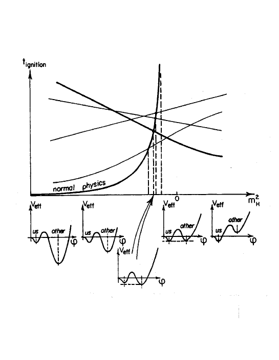
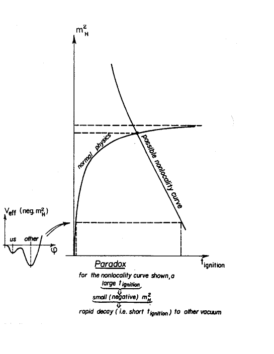
Let us first use “normal physics” to see how the relative depths of the two minima of the double well are related to $m^{2}_{Higgs}$ and to $t_{ignit}$. It can be deduced frombennett7 that a large negative value of $m^{2}_{Higgs}$ corresponds to the relative minimum $V_{eff}(\phi_{other})$ being deeper than $V_{eff}(\phi_{us})$ (in which by assumption the Universe starts off following Big Bang) than for less negative values of $m^{2}_{Higgs}$ (see Fig. 16). It can also be argued quite plausibly that a minimum in $V_{eff}$ at $\phi_{other}$ much deeper than that at $\phi_{us}$ would correspond to an early (small) $t_{ignit}$ inasmuch as the “false” vacuum at $\phi_{us}$ would be very unstable. However, as the value of the potential at $\phi_{other}$ approaches that at $\phi_{us}$, $t_{ignit}$ becomes longer and longer and approaches infinity as the values of $V_{eff}$ at $\phi_{us}$ and $\phi_{other}$ become the same. The development of the double well potential and $m^{2}_{Higgs}$ as a function of $t_{ignit}$ is illustrated in Fig. 16. Note that the larger the difference $|V_{eff}(\phi_{other})-V_{eff}(\phi_{us})|$ the more the realization of say $I_{fixed\;2}$ will in general depend on $t_{ignit}$. If $V_{eff}(\phi_{us})=V_{eff}(\phi_{other})$, $t_{ignit}$ plays no role in realizing e.g. $I_{fixed\;2}$ and the value of $m^{2}_{Higgs}$ becomes independent of $t_{ignit}$.

48 Avoiding paradoxes arising from non-locality

In general the presence of non-locality leads to paradoxes. While the form that the non-local action (or potential $V_{nl}$ in this discussion) is unknown to us, we make the 4 generically representative guesses portrayed as the 4 non-locality curves in Fig. 16. In particular, non-locality curves having a negative slope as a function of $t_{ignit}$ lead to paradoxes in the following manner. Consider the non-locality curve in Fig. 16 drawn with bold line that is redrawn in a rotated position in Fig. 17. Let us make the assumption that $t_{ignit}$ is large and see that this leads to a contradiction. Assuming that $t_{ignit}$ is large, it is seen from the non-locality function in Fig. 17 (call it $m^{2}_{Higgs\;nl}(t_{ignit})$ to distinguish it from the “normal physics” $m_{Higgs}^{2}(t_{ignit})$) that this implies that the “normal physics” $m^{2}_{Higgs}$ has a large negative value. But a large negative value of $m^{2}_{Higgs}$ corresponds in “normal physics”to a (false) vacuum at $\phi_{us}$ that is very unstable and therefore to a very short $t_{ignit}$ corresponding to a rapid decay to the stable vacuum at $\phi_{other}$. So the paradox appears: the assumption of a large $t_{ignit}$ implies a small $t_{ignit}$. This happens because in general $m^{2}_{Higgs}(t_{ignit})\neq m^{2}_{Higgs\;nl}(t_{ignit})$ and is akin to the “matricide” paradox encountered for example when dealing with “time machines”. It is well knownbennett8 ; bennett9 ; bennett10 that Nature avoids such paradoxes by choosing a very clever solution in situations where these paradoxes lure.

In the case of the paradoxes that can come about due to non-locality of the type considered here, a clever solution that avoids paradoxes is available to Nature in the form of the Multiple Point Principle (MPP). The MPP solution corresponds to the intersection of the “normal physics” curve and the “non-locality curve” in Fig. 17. because here the vacua at $\phi_{us}$ and $\phi_{other}$ are (essentially) degenerate. But at this intersection point, $m_{Higgs}^{2}(t_{ignit})=m^{2}_{Higgs\;nl}(t_{ignit})$ so the paradox is avoided. So the paradox is avoided at the multiple point. But at the multiple point, an intensive parameter has its value fine-tuned for a wide range of values of the conjugate extensive quantity. Fine-tuning can therefore be understood as a consequence of Nature’s way of avoiding paradoxes that can come about due to non-locality.

It should be pointed out that the paradox-free solution corresponding to the intersection of the two curves in Fig. 17 occurs for a value of $m^{2}_{Higgs}$ corresponding to “our” vacuum at $\phi_{us}$ being very slightly unstable. The value of $m^{2}_{Higgs}$ corresponding to the vacua at $\phi_{us}$ and $\phi_{other}$ being (precisely) degenerate is slightly less negative than that corresponding to the multiple point value of $m^{2}_{Higgs}$ at the intersection of the curves. Note that the multiple point value of $m^{2}_{Higgs}$ is very insensitive to which “guess” we use for the non-local action. Indeed all the “non-locality” curves in Fig. 16 intersect the “normal physics” curve at values of $m^{2}_{Higgs}$ that are tightly nested together. The reason for this is that $m^{2}_{Higgs}$ is a very slowly varying function of $t_{ignit}$ as $m_{Higgs}^{2}(t_{ignit})$ approaches the value corresponding to degenerate vacua. The more nearly parallel the “normal physics” and the “non-locality” curves at the point of intersection, the less are the (paradoxical) effects of non-locality. For a point of intersection at values of $t_{ignit}$ sufficiently large that (the “normal physics”) $m^{2}_{Higgs}(t_{ignit})\approx m^{2}_{Higgs}(\infty)$, the non-locality effects disappear as the curves become parallel since both curves become independent of $t_{ignit}$. If the curves were parallel, there would also be the possibility that these do not intersect in which case there would be no “miraculous solution” that could avoid the paradoxes imbued in having non-locality.

If the interval $|\phi^{2}_{other}$-$\phi^{2}_{us}|$ is large (e.g. of the order of the largest physically conceivable scale (Planck?) if tuning is to be maximally effective) and if $I_{fixed\;2}$ falls not too close to the ends of this interval, then $t_{ignit}$ will be something of the order of half the life of the universe. Actually, the approximate degeneracy of the vacua $V_{eff}(\phi_{us})\approx V_{eff}(\phi_{other})$ may be characteristic of the temperature of the post-Big Bang universe in the present epoch and not characteristic of the high temperature that prevailed immediately following the Big Bang. At high temperatures, the free energy is considerably less than the total energy if the entropy is large enough. A phase with a large number of light particles - for example a Coulomb-like vacuum such as the “us” phase in which we live - could very plausibly be so strongly favoured at high temperatures that other phases - for example the “other” vacuum - simply disappeared at the high temperature of the universe immediately following the Big Bang.

If this were to have depleted the universe of the phase having $\phi_{other}$ at high temperatures, it would indeed be difficult to re-establish it in a lower temperature universe even if the vacuum at $\phi_{us}$ were to be only meta-stable and the vacuum at $\phi_{other}$ were the true vacuum at the lower temperature. Such an exchange of the true vacuum is indeed a possibility in going to lower temperatures inasmuch as the difference between the total energy and the free energy decreases in going to lower temperatures. Accordingly this difference becomes less effective in favouring a Coulomb-like phase at the expense of a phase with heavier particles.

At this point we point out that when we say the “vacuum at $\phi_{us}$” and “vacuum at $\phi_{other}$” we are thinking of the approximation $\phi=\phi_{us}$ and $\phi=\phi_{other}$ almost everywhere and at all times in respectively the early and late epochs of the universe in our discussion. More correctly we should talk about vacuum densities $\langle\phi(x^{0},\mathchoice{\mbox{\boldmath$\displaystyle x$}}{\mbox{\boldmath$\textstyle x$}}{\mbox{\boldmath$\scriptstyle x$}}{\mbox{\boldmath$\scriptscriptstyle x$}})\rangle_{us}$ and $\langle\phi(x^{0},\mathchoice{\mbox{\boldmath$\displaystyle x$}}{\mbox{\boldmath$\textstyle x$}}{\mbox{\boldmath$\scriptstyle x$}}{\mbox{\boldmath$\scriptscriptstyle x$}})\rangle_{other}$ where

$$\langle\phi(x^{0},\mathchoice{\mbox{\boldmath$\displaystyle x$}}{\mbox{\boldmath$\textstyle x$}}{\mbox{\boldmath$\scriptstyle x$}}{\mbox{\boldmath$\scriptscriptstyle x$}})\rangle_{us}\stackrel{{\scriptstyle def}}{{=}}\frac{1}{V_{us}}\int_{t_{BB}}^{t_{ignit}}dx^{0}\int d^{3}\mathchoice{\mbox{\boldmath$\displaystyle x$}}{\mbox{\boldmath$\textstyle x$}}{\mbox{\boldmath$\scriptstyle x$}}{\mbox{\boldmath$\scriptscriptstyle x$}}\sqrt{g(x)}\phi(x^{0},\mathchoice{\mbox{\boldmath$\displaystyle x$}}{\mbox{\boldmath$\textstyle x$}}{\mbox{\boldmath$\scriptstyle x$}}{\mbox{\boldmath$\scriptscriptstyle x$}})$$

where $V_{us}$ denotes the the 4-volume of the universe in the first epoch. Density $\langle\phi(x^{0},\mathchoice{\mbox{\boldmath$\displaystyle x$}}{\mbox{\boldmath$\textstyle x$}}{\mbox{\boldmath$\scriptstyle x$}}{\mbox{\boldmath$\scriptscriptstyle x$}})\rangle_{other}$ is defined analogously. The more correct $\langle\phi(x^{0},\mathchoice{\mbox{\boldmath$\displaystyle x$}}{\mbox{\boldmath$\textstyle x$}}{\mbox{\boldmath$\scriptstyle x$}}{\mbox{\boldmath$\scriptscriptstyle x$}})\rangle_{us}$ is mentioned here so as not to confuse the reader when we talk about the changes in $V_{eff}(\phi_{us}(x^{0},\mathchoice{\mbox{\boldmath$\displaystyle x$}}{\mbox{\boldmath$\textstyle x$}}{\mbox{\boldmath$\scriptstyle x$}}{\mbox{\boldmath$\scriptscriptstyle x$}}))$ as the universe cools following Big Bang.

Recall now that the value of say of $I_{fixed\;2}$ can easily (i.e. as a generic possibility) assume a value that requires that the universe to be in the “phase” with $\langle\phi(x^{0},\mathchoice{\mbox{\boldmath$\displaystyle x$}}{\mbox{\boldmath$\textstyle x$}}{\mbox{\boldmath$\scriptstyle x$}}{\mbox{\boldmath$\scriptscriptstyle x$}})\rangle_{other}$ during a sizeable part of its life if the universe is to have multiple point parameters in the course of its evolution (as required for avoiding the paradoxes that accompany non-locality). How can Nature overcome the energy barrier that must be surmounted in order to bring about the decay of the slightly unstable (false) vacuum with $\langle\phi(x^{0},\mathchoice{\mbox{\boldmath$\displaystyle x$}}{\mbox{\boldmath$\textstyle x$}}{\mbox{\boldmath$\scriptstyle x$}}{\mbox{\boldmath$\scriptscriptstyle x$}})\rangle_{us}$ to the vacuum with $\langle\phi(x^{0},\mathchoice{\mbox{\boldmath$\displaystyle x$}}{\mbox{\boldmath$\textstyle x$}}{\mbox{\boldmath$\scriptstyle x$}}{\mbox{\boldmath$\scriptscriptstyle x$}})\rangle_{other}$? Even producing just a tiny “seed” of the “true” vacuum having $\langle\phi(x^{0},\mathchoice{\mbox{\boldmath$\displaystyle x$}}{\mbox{\boldmath$\textstyle x$}}{\mbox{\boldmath$\scriptstyle x$}}{\mbox{\boldmath$\scriptscriptstyle x$}})\rangle_{other}$ would be very difficult. What miraculously clever means can Nature devise so as to avoid deviations from a multiply critical evolution of the universe? One ingenious master plan that Nature may have implemented is the creation of life with the express “purpose” of evolving some (super intelligent?) physicists that could ignite a “vacuum bomb” by first creating in some very expensive accelerator the required “seed” of the “correct” vacuum having $\langle\phi(x^{0},\mathchoice{\mbox{\boldmath$\displaystyle x$}}{\mbox{\boldmath$\textstyle x$}}{\mbox{\boldmath$\scriptstyle x$}}{\mbox{\boldmath$\scriptscriptstyle x$}})\rangle_{other}$ that subsequently would engulf the universe in a (for us) cataclysmic transition to the “other” phase thereby permitting the continued evolution of a “paradox-free” universe!

49 Conclusion

We attempt to justify the assertion that fine-tuning in Nature seems to imply a fundamental form of non-local interaction. This could be manifested in a phenomenologically acceptable form as everywhere in spacetime identical interactions between any pair of spacetime points. This would be implemented by requiring the non-local action to be diffeomorphism invariant.

Next we put forth our multiple point principle which states that coupling parameters in the Standard Model tend to assume values that correspond to the values of action parameters lying at the junction of a maximum number of regulator induced phases (e.g., so-called “lattice artifact phases”) separated from one another in action parameter space by first order transitions. The action which of course is defined on a gauge group (e.g., the non-simple SM gauge group) governs fluctuation patterns along the various subgroup combinations $(K,H)$ with $H\lhd K\subseteq G$ that characterize the phases that come together at the multiple point. We then consider extensive quantities that are functions of functionals $I_{f_{j}}[\phi(x)]$ that are essentially Feymann path histories of the Universe for functions $f_{j}(\phi)$ of the fields $\phi(x)$ and derivatives of these fields. We then think of the generic situation in which these extensive quantities can happen to be fixed at values that require the universe to be realized as two or more coexisting phases. We draw on the analogy to the forced coexistence of ice and liquid water that occurs for a whole range of possible total energies because of the finite heat of melting (first order phase transition). With our multiple point principle, the intensive quantities (couplings) conjugate to extensive quantities fixed in this way become fine-tuned in a manner analogous to the fine tuning of temperature to $0^{o}C$ when the total energy of a system of $H_{2}O$ can only be realized as coexisting ice and liquid phases.

One generic way of having coexisting phases in a quantum field theory in 3+1 dimensions would be to have different phases in different epochs of the lifetime of the Universe with phase transitions occuring at various times in the course of the lifetime of the Universe. If the transitions were first order, one would have fine-tuning of (intensive) couplings conjugate to extensive quantitity values that can only be realized by having coexisting (i.e., more than one) phases. But such a fine-tuning would involve non-locality: the fine-tuned values of coupling constants would depend on future phase transitions into phases that do not even exist at the time such couplings are fine-tuned.

Even non-locality of this sort (i.e., non-localy manifested as a diffeomorphism invariant non-local action) can lead to paradoxes of the “matricide paradox” type. We argue that such paradoxes are avoided when Nature chooses the multiple point principle solution to the problem of finetuning.

*Dynamics of Glue-Balls in $N=1$ SYM Theory Luzi Bergamin

50 Introduction

The low energy effective action of $N=1$ SYM theory is written in terms of a chiral effective field $S=\varphi+\theta\psi+\theta^{2}F$, which may be defined from the local source extension of the SYM action veneziano82 ; Shore:1983kh ; burgess95 ; bergamin01

$$S \propto\frac{\delta}{\delta J}W[J,\bar{J}]\ , e^{iW[J,\bar{J}]} =\int\!\!\mathcal{D}V\;\;e^{i\int\!\!d^{4}xd^{2}\theta\;(J+\tau_{0})\operatorname{Tr}W^{\alpha}W_{\alpha}+\operatorname{h.c.}}\ .$$ (136)

With appropriate normalization $S$ is equivalent to the anomaly multiplet $\bar{D}^{\dot{\alpha}}V_{\alpha\dot{\alpha}}=D_{\alpha}S$. $J(x)$ is the chiral source multiplet, with respect to which a Legendre transformation can be defined burgess95 ; bergamin01 . The resulting effective action is formulated in terms of the gluino condensate $\varphi\propto\operatorname{Tr}\lambda\lambda$, the glue-ball operators $F\propto\operatorname{Tr}F_{\mu\nu}F^{\mu\nu}+i\operatorname{Tr}F_{\mu\nu}\tilde{F}^{\mu\nu}$ and a spinor $\psi\propto(\sigma^{\mu\nu}\lambda)_{\alpha}F_{\mu\nu}$. An effective Lagrangian in terms of this effective field $S$ has the form veneziano82 ; Shore:1983kh

$$\mathcal{L}_{\mbox{\scriptsize{eff}}}=\int\!\!\mbox{d}^{4}\theta\;K(S,\bar{S})-\Bigl{(}\int\!\!\mbox{d}^{2}\theta\;S(\log\frac{S}{\Lambda^{3}}-1)+\operatorname{h.c.}\Bigr{)}\ .$$ (137)

The correct anomaly structure is realized by the superpotential and thus $K(S,\bar{S})$ is invariant under all symmetries. In ref. veneziano82 the explicit ansatz $K=k(\bar{S}S)^{1/3}$ had been made, which leads to chiral symmetry breaking due to $\langle S\rangle=\Lambda^{3}$, but supersymmetry is not broken as $\varphi$ and $\psi$ acquire the same mass $m=\Lambda/k$.

51 Glue-balls and constraint Kähler geometry

Though the spectrum found in ref. veneziano82 does not include any glue-balls, such fields do appear in $F$. However, they drop out in the analysis of veneziano82 , as $F$ is treated as an auxiliary field. Indeed, the highest component of a chiral superfield is auxiliary in standard SUSY non-linear $\sigma$-models, i.e. there appear no derivatives acting onto this field and moreover its potential is not bounded from below, but from above. In case of the Veneziano-Yankielowicz Lagrangian the part depending on the auxiliary field reads

$$\mathcal{L}_{\mbox{\scriptsize{aux}}}=k(\bar{\varphi}\varphi)^{-\frac{2}{3}}\bar{F}F+\Bigl{(}\frac{1}{3}\varphi^{-\frac{2}{3}}\bar{\varphi}^{-\frac{5}{3}}F\bar{\psi}\bar{\psi}-F\log\frac{\varphi}{\Lambda^{3}}+\operatorname{h.c.}\Bigr{)}\ ,$$ (138)

and the supersymmetric spectrum is obtained, if and only if $F$ is eliminated by the algebraic equations of motion that follow from (138). This leads to the unsatisfactory result that glue-balls cannot be introduced in a straightforward way (cf. also farrar98 ) which, in addition, contradicts available lattice-data Peetz:2002sr .

However, in the special case of $N=1$ SYM the elimination of $F$ is not consistent: If $F$ is eliminated from (138), this implies that the theory must be ultra-local in the field $F$ exactly, i.e. even corrections to the effective Lagrangian which are not included in (137) are not allowed to change the non-dynamical character of $F$. If this field would be related to the fundamental auxiliary field, this restriction would be obvious. But in $N=1$ SYM the situation is different: $S$ is the effective field from a composite operator and $F$ is not at all related to the fundamental auxiliary field $D$. As a consequence, the restriction of ultra-locality on $F$ leads to an untenable constraint on the physical glue-ball operators (for details we refer to bergamin01 ; bergamin02:1 ; Bergamin:2003ub ).

As shown in ref. Shore:1983kh , the effective Lagrangian of veneziano82 is not the most general expression compatible with all the symmetries, but the constant $k$ may be generalized to a function $k(\frac{S^{1/3}}{\bar{D}^{2}\bar{S}^{1/2}},\frac{\bar{S}^{1/3}}{D^{2}S^{1/2}})$. This non-holomorphic part automatically produces space-time derivatives onto the field $F$, which is most easily seen when $K(S,\bar{S})$ is rewritten in terms of two chiral fields Bergamin:2003ub :

$$K(S,\bar{S})\rightarrow K(\Psi_{0},\Psi_{1};\bar{\Psi}_{0},\bar{\Psi}_{1})$$ (139)

$\Psi_{0}$ and $\Psi_{1}$ are not independent, but they must obey the constraints

$$\Psi_{0} =S^{\frac{1}{3}}=\varphi^{\frac{1}{3}}+\frac{1}{3}\varphi^{-\frac{2}{3}}\theta\psi+\frac{1}{3}\theta^{2}(\varphi^{-\frac{2}{3}}F+\frac{1}{3}\varphi^{-\frac{5}{3}}\psi\psi)\ ,$$ (140)

$$\Psi_{1} =\bar{D}^{2}\bar{\Psi}_{0}=\frac{1}{3}(\bar{\varphi}^{-\frac{2}{3}}\bar{F}+\frac{1}{3}\bar{\varphi}^{-\frac{5}{3}}\bar{\psi}\bar{\psi})-\frac{i}{3}\theta\sigma^{\mu}\partial_{\mu}(\bar{\varphi}^{-\frac{2}{3}}\bar{\psi})-\theta^{2}\Box\bar{\varphi}^{\frac{1}{3}}\ .$$ (141)

As $F$ appears as lowest component of $\bar{\Psi}_{1}$, the Lagrangian includes a kinetic term for that field. In contrast to the situation in veneziano82 , this is not inconsistent as the potential in $F$ may include arbitrary powers in that field (instead of a quadratic term only) and can be chosen to be bounded from below (instead of above). This way the field $F$ is promoted to a usual physical field. It has been shown in bergamin02:1 that there exist consistent models of this type. In Bergamin:2003ub these ideas have been applied to $N=1$ SYM, leading to an effective action of that theory with dynamical glue-balls as part of the low-energy spectrum. Formally, the effective potential looks the same as in the case of Veneziano and Yankielowicz:

$$\begin{split}V_{\mbox{\tiny eff}}&=-\tilde{g}_{\varphi\bar{\varphi}}F\bar{F}+\frac{1}{2}\tilde{g}_{\varphi\bar{\varphi},\bar{\varphi}}F(\bar{\psi}\bar{\psi})+\frac{1}{2}\tilde{g}_{\varphi\bar{\varphi},\varphi}\bar{F}(\psi\psi)-\frac{1}{4}\tilde{g}_{\varphi\bar{\varphi},\varphi\bar{\varphi}}(\psi\psi)(\bar{\psi}\bar{\psi})\\[3.01385pt] &\quad+c\bigl{(}F\log\frac{\varphi}{\Lambda^{3}}+\bar{F}\log\frac{\bar{\varphi}}{\bar{\Lambda}^{3}}-\frac{1}{2\varphi}(\psi\psi)-\frac{1}{2\bar{\varphi}}(\bar{\psi}\bar{\psi})\bigr{)}\end{split}$$ (142)

However, in contrast to reference veneziano82 the Kähler “metric” is a function of $\varphi$ and $F$, $\tilde{g}_{\varphi\bar{\varphi}}(\varphi,F;\bar{\varphi},\bar{F})$. From eq. (142) the consistent vacua can be derived, for explicit expressions we refer to Bergamin:2003ub . The most important properties of the Lagrangian (137) with (139) are:

The effective potential is minimized with respect to all fields $\varphi$, $\psi$ and $F$. Consequently, the dominant contributions that stabilize the potential must stem from the Kähler part, not from the superpotential: The superpotential is a holomorphic function in its fields and therefore its scalar part must have unstable directions. In the present context there exists no mechanism to transform these instabilities into stable but non-holomorphic terms.

Though the model has the same superpotential as the Lagrangian of ref. veneziano82 its spectrum is completely different: Chiral symmetry breaks by a vacuum expectation value (vev) of $\varphi\propto\Lambda^{3}$, but this mechanism is more complicated than in veneziano82 . Any stable ground-state must have non-vanishing vev of $F$. But $\langle F\rangle$ is the order parameter of supersymmetry breaking and thus this symmetry is broken as well. $\psi$ is a massless spinor, the Goldstino.

The supersymmetry breaking scenario is of essentially non-perturbative nature: it is not compatible with perturbative non-renormalization theorems, as the value of $V_{\mbox{\tiny eff}}$ in its minimum and the vev of ${T^{\mu}}_{\mu}$ are no longer equivalent. In particular, the former can be negative, while the latter is positively semi-definite due to the underlying current-algebra relations. To our knowledge this is the first model, where this type of supersymmetry breaking has found a concrete description (cf. bergamin02:1 ; Bergamin:2003ub for details).

Any ground state with $\langle\tilde{g}_{\varphi\bar{\varphi}}\rangle\neq 0$ can be equipped with stable dynamics for $p^{2}<|\Lambda|^{2}$. In the construction of concrete kinetic terms it is important to realize that (139) may include expressions with explicit space-time derivatives. Again this is possible as $F$ is not interpreted as an auxiliary field.

In summary, the Lagrangian of ref. Bergamin:2003ub is the most general one, which can be formulated in terms of the effective field $S$. Consistent ground-states can be found together with broken supersymmetry only. It would be interesting to compare these results with a different action, which has supersymmetric ground-states. But the ”pièce de résistance” for such an action is the fact, that it cannot start from the effective field $S$.

Acknowledgements

The author would like to thank U. Ellwanger, J.-P. Derendinger, E. Kraus, P. Minkowski, Ch. Rupp and E. Scheidegger for interesting discussions. This work has been supported by the Austrian Science Foundation (FWF) project P-16030-N08.

*Quantization of Systems with Continuous Symmetries on the Classical Background: Bogoliubov Group Variables Approach Margarita V. Chichikina

52 Introduction

In present article the theory of quantization of nonlinear boson fields in a vicinity a nontrivial classical component by means of the Bogoliubov group variables is reprezented. Among canonical transformations of a boson field always there is an separation $c$-numerical component, therefore operator of a boson field always potentially contains a classical boson field. Therefore quantization of any nonlinear physical system should include quantization of a boson field in a vicinity of a classical background. If it is possible to suppose this field small, connected with it the effects, as a rule, are satisfactorily described in the framework of standart perturbation theory, when the classical field is as a first approximation considered equal to zero. If it is impossible to consider a classical field from the very beginning small (gravitation and extended particles), there is a task of the description of properties of physical system, in which main effect is the separation of a classical boson field.

The theories, existing on at present moment, of quantization on a classical background meet two basic difficulties. Firstly, — and this main — a problem of the conservation laws. The second difficulty of quantization on a classical background is the zero-mode problem. To bypass these problems we propose to use idea of the Bogoliubov, which was proposed in work of N.N.Bogoliubov. He has proposed to carry out quantization in the terms new variable. The transformations of the Bogoliubov are widely used in a quantum field theory. However, if the group of invariancy of system includes transformation of time, there are difficulties, connected with following: for reception of expression for Hamiltonian as generator of time translation it is necessary to know equations of motion, and for record of equations of motion in an explisit form it is necessary to know expression for Hamiltonian. This difficulty seriously limited a field of application of the Bogoliubov group variables, since did not enable to consider non-stationary systems.

In this work we propose quantizations, new a way, which will allow to use the Bogoliubov group variables for systems having arbitrary symmetry group (provided that we we know representation of this group), including for non-stationary systems.

53 The basic ideas of a new method of quantization

In this section we represent schematically the basic ideas of quantization of boson fields by means of method of the Bogoliubov group variables. Firstly we pass to new variable - Bogoliubov group variables - and all considered quantities we express in the terms new variable.

Let variable $x^{{}^{\prime}}$ are related to $x$ by group transformation:

$$x^{\prime}=F(x,a),\qquad x^{\prime\prime}=F\left(F(x,a),b\right)=F(x,c),\qquad c=\varphi\left(a,b\right).$$

Variations of coordinates at a variation of parameters of group $a$ are:

$$\left(\delta x^{\prime}\right)^{i}=\xi_{s}^{i}(x^{\prime})B_{p}^{s}(a)\delta a^{p},$$

where $i=0,1,2,3$- number of coordinate, $p=1...,r$, and $k$ - number of generators of group. The group properties of transformation are defined by tensor $B_{p}^{s}(a)$.

Let’s define Bogoliubov transformation as follows:

$$f(x)=gv(x^{{}^{\prime}})+u(x^{{}^{\prime}}),$$

dimensionless parameter $g$ is supposed to be large, and $(u(x^{{}^{\prime}}),a)$ are independent new variable (Bogoliubov group variable). Explisitly separated large component depends on $x^{{}^{\prime}}$ as well as a quantum part. Thus we restore invariancy with respect to transformations group, which was broken by explisit separation of classical component, as it was pointed out in introduction. However consideration of variable $\tau$ as independent leads to the fact that right-hand side of our equation contains now on $k$ variable more than left one. In order to equalize the number of variables we impose on $u(x^{{}^{\prime}})$ some invariant conditions.

Secondly we develop the perturbation theory. All integrals of motions are expressed in new variables. Analyzing received expressions, we obtain conditions, at which application of perturbation theory is correct, namely: the classical part owes to satisfy to some equations. These equations turn out coinside with Eileur-Lagrange equations. However this result is not trivial: it was received not as a consequence of variational principle, but as a condition of development of a perturbative scheme for our system in the terms new variables, while for reception of these equations we did not need to know Hamiltonian structure as generator of transaltions on time.

So, at the second stage we obtain equations of motion for classical components.

And then we construct of system state space . At this stage of construction of our scheme we achieve correct number of degrees of freedom which will be equal to its real number. During realization of a reduction we obtain equations of motion for quantum correction for our field (the equations appear nonlinear). Also at this stage the explisit expressions for creation-annihilation operators of quantums of a field are obtained as well as and spectrum of frequencies, that is actually, energy spectrum. Besides we obtain expressions for integrals of motion as generators of corresponding symmetry transformations:

$$O_{0}=i\Im^{\alpha}{\partial\over\partial\tau^{\alpha}},$$

In particular, hamiltonian is generator of shift on time. Let’s note, that equations of motion of a classical part and explisit form of hamiltonian are received independently, that is is overcome basic difficulty of the description of non-stationary systems, which was described in introduction.

Also in zero order we shall obtain Heizenberg equation in the terms new variables.

Totality of the received results:

• Equation of motion of a classical part;

• Equation of motion of the quantum additive;

• Energy spectrum;

• Expressions for integrals of a motion;

• Heisenberg equations;

• Explicit expression for the field operator;

allows to assert, that our theory gives the complete description of system of boson fields, quantized on classical background. While theory guarantees exact performance of the conservation laws in any order of perturbation theory and also allows to avoid a zero-mode problem.

*Singular Compactifications and CosmologyWork supported by the ‘Schwerpunktprogramm Stringtheorie’ of the DFG. Laur Järv, Thomas Mohaupt and Frank Saueressig

During the last year a lot of effort has been made to explain the astronomical evidence for an inflationary epoch of the early universe and the current modest accelerated expansion by invoking a scalar potential derived from string or M-theory compactifications. So far two mechanisms leading to potentials viable to describe accelerated cosmological expansion have been explored Emp&Tow : (i) compactifications on hyperbolic spaces hyper_comp and (ii) compactifications with fluxes flux_comp . Our recent work model ; cosmo gives the first example of (iii) compactification on a singular internal manifold.

In the case of smooth compactifications one usually has a moduli space of vacua corresponding to the deformations of the internal manifold $X$ and the background fields. For theories with eight or less supercharges this moduli space includes special points where $X$ degenerates, rendering the corresponding low energy effective action (LEEA) discontinuous or singular. However, within the full string or M-theory these singularities are believed to be artifacts, which result from ignoring some relevant modes of the theory, namely the winding states of strings or branes around the cycles of $X$. Singularities of $X$ arise when such cycles are contracted to zero volume, thereby introducing additional massless states. Incorporating these states leads to a smooth gauged supergravity action which entails a scalar potential.

In Calabi-Yau (CY) compactifications of M-theory undergoing a topological flop transition these additional states (‘transition states’) are given by $N$ charged hypermultiplets which become massless at the transition locus. There are two ways to include the effect of these extra states in the LEEA. The usual LEEA is obtained by dimensional reduction on the smooth CY and contains only states which are generically massless. The flop manifests itself in a discontinuous change of the vector multiplet couplings at the transition locus. We call this description the ‘Out-picture’ since the extra states are left out. On the contrary, the ‘In-picture’ is obtained by including the transition states as dynamical fields in the Lagrangian.

In model we constructed an In-picture LEEA for a generic M-theory flop by combining knowledge about the general ${\cal N}=2,D=5$ gauged supergravity action with information about the extra massless states. While the vector multiplet sector could be treated exactly we used a toy model based on the quaternion-Kähler manifolds $\frac{U(1+N,2)}{U(1+N)\times U(2)}$ to describe the hypermultiplet sector. In order to find the gauging describing the flop we worked out the metrics, the Killing vectors, and the moment maps of these spaces. This data enabled us to construct a unique LEEA which has all the properties to model a flop: the extra hypermultiplets acquire a mass away from the transition locus while the universal hypermultiplet remains massless.

In cosmo we considered an explicit model for a CY compactification undergoing a flop with $N=1$ and investigated the effect of the transition states on five-dimensional Kasner cosmologies,

$$ds^{2}=-d\tau^{2}+e^{2\alpha(\tau)}d\mathchoice{\mbox{\boldmath$\displaystyle x$}}{\mbox{\boldmath$\textstyle x$}}{\mbox{\boldmath$\scriptstyle x$}}{\mbox{\boldmath$\scriptscriptstyle x$}}^{2}+e^{2\beta(\tau)}dy^{2}\;.$$ (143)

Comparing the cosmological solutions of the Out- and the In-picture, we found that the inclusion of the dynamical transition states has drastic consequences for moduli stabilization and accelerated expansion.

As soon as we allow all light states to be excited the scalar fields no longer show the usual run-away behavior but are attracted to the flop region where they oscillate around the transition locus. Thus the “almost singular” manifolds close to the flop are dynamically preferred. This is somewhat surprising, because the potential has still many unlifted flat directions meaning there is no energy barrier which prevents the system from running away. Hence this effect cannot be predicted by just analyzing the critical points of the superpotential. The following thermodynamic analogy helps to explain the situation. Generically the available energy of the system is distributed equally among all the light modes (“thermalization”). Thus near the flop line the additional degrees of freedom get their natural share of it. Once this has happened, it becomes very unlikely that the system “finds” the flat directions and “escapes” from the flop region. Our numerical solutions confirm this picture: irrespective of the initial conditions the system finally settles down in a state where all the fields either approach finite values or oscillate around the transition region with comparable and small amplitudes. From time to time one sees “fluctuations from equilibrium”, i.e., some mode picks up a bigger share of the energy for a while, but the system eventually thermalizes again. In an ideal scenario of moduli stabilization, however, one would like to have a damped system so that the moduli converge to fixed point values.

The second important aspect is that the scalar potential of the In-picture induces short periods of accelerated expansion in the three-space. Yet the net effect of the accelerating periods on cosmic expansion is not very significant. Again, this feature can be understood qualitatively in terms of the properties of the scalar potential. The point is that the potential is only flat along the unlifted directions while along the non-flat ones it is too steep to support sustained accelerated expansion. Transient periods of acceleration occur when the scalar fields pass through their collective turning point, where running “uphill” the potential turns into running “downhill” and the potential energy momentarily dominates over the kinetic energy. To get a considerable amount of inflation via a slow-roll mechanism, one would need to lift some of the flat directions gently without making them too steep.

In summary we see that the dynamics of the transition states is interesting and relevant, and can be part of the solution of the problems of moduli stabilization and inflation. One direction for further investigations is to consider more general gaugings of our five-dimensional model. Once gaugings leading to interesting cosmological solutions are found, one should clarify whether these can be derived from string or M-theory where they correspond to adding fluxes or branes. Another direction is to extend our construction to other topological transitions. In particular it would be interesting to study the effect of transition states on four-dimensional cosmologies arising, e.g., from type II compactifications on singular CY manifolds. It is conceivable that a realistic cosmology derived from sting or M-theory will have to include both the effects of fluxes and branes, and the possibility of internal manifolds becoming singular.

*Fundamental Physics and Lorentz Violation Ralf Lehnert

54 Introduction

On the one hand, the Standard Model (SM) of particle physics is extremely successful phenomenologically. On the other hand, this conference is called What Comes Beyond the Standard Model because it is generally believed that the SM is really the low-energy limit of a more fundamental theory incorporating quantum gravity. Experimental research in this field faces various challenges. They include the expected Planck suppression of quantum-gravity signatures and the absence of a realistic underlying framework.

A promising approach for progress in quantum-gravity phenomenology is the identification of relations that satisfy three principle criteria: they must hold exactly in known physics, they are expected to be violated in candidate fundamental theories, and they must be testable with ultra-high precision. Spacetime symmetries satisfy all of these requirements. Lorentz and CPT invariance are key features of currently accepted fundamental physics laws, and they are amenable to Planck-sensitivity tests. Moreover, Lorentz and CPT breakdown has been suggested in a variety of approaches to fundamental physics. We mention low-energy emergent Lorentz symmetry np83 , strings kps , spacetime foam ell98 , nontrivial spacetime topology klink , loop quantum gravity amu , noncommutative geometry chklo , and varying couplings klp03 . The latter of these mechanism will be discussed in more detail in this talk.

At presently attainable energies, Lorentz and CPT violating effects are described by a general extension of the SM. The idea is to include into the SM Lagrangian Lorentz and CPT breaking operators of unrestricted dimensionality only constrained by coordinate independence sme . This Standard-Model Extension (SME) has provided the basis for many investigations placing bounds on Lorentz and CPT violation. For the best constraints in the matter and photon sectors, see Ref. bear and Refs. cfj ; km , respectively. Note that certain Planck-suppressed SME operators for Lorentz and CPT breaking provide alternative explanations for the baryon asymmetry in our universe bckp and the observed neutrino oscillations neu .

55 Lorentz violation through varying couplings

Early speculations in the subject of varying couplings go back to Dirac’s numerology lnh . Subsequent theoretical investigations have shown that time-dependent couplings arise naturally in many candidate fundamental theories theo . Recent observational claims of a varying fine-structure parameter $\alpha$ webb have led to a renewed interest in the subject jpuzan .

Varying couplings are associated with spacetime-symmetry violations. For instance, invariance under temporal and/or spatial translations is in general lost. Since translations are closely interwoven with the other spacetime transformations in the Poincaré group, one anticipates that Lorentz symmetry might be affected as well. This is best illustrated by an example. Consider the Lagrangian ${\cal L}$ of a complex scalar $\Phi$, and suppose a spacetime-dependent parameter $\xi(x)$ is coupled to the kinetic term: ${\cal L}\supset\xi\partial_{\mu}\Phi\partial^{\mu}\Phi^{*}$. An integration by parts yields ${\cal L}\supset-\Phi(\partial_{\mu}\xi)\partial^{\mu}\Phi^{*}$. If, for instance, $\xi$ varies smoothly on cosmological scales, $(\partial_{\mu}\xi)=k_{\mu}$ is essentially constant locally. The Lagrangian then contains a nondynamical fixed 4-vector $k_{\mu}$ selecting a preferred direction in the local inertial frame violating Lorentz symmetry.

The above example can be generalized to other situations. For instance, non-scalar fields can play a role, and Lorentz violation can arise through coefficients like $k_{\mu}$ in the equations of motion or in subsidiary conditions. Note that the Lorentz breaking is independent of the chosen reference frame: if $k_{\mu}\neq 0$ in a particular set of local inertial coordinates, $k_{\mu}$ is nontrivial in any coordinate system. In the next section, we show that varying couplings can arise through scalar fields acquiring expectations values in a cosmological context. Note, however, that the above argument for Lorentz violation is independent of the mechanism driving the variation of the coupling.

56 Four-dimensional supergravity cosmology

Consider a Lagrangian ${\cal L}$ with two real scalars $A$ and $B$ and a vector $F^{\mu\nu}$:

$$\frac{4{\cal L}}{\sqrt{g}} = \frac{{\partial_{\mu}A\partial^{\mu}A+\partial_{\mu}B\partial^{\mu}B}}{B^{2}}-2R-MF_{\mu\nu}F^{\mu\nu}-NF_{\mu\nu}\tilde{F}^{\mu\nu}\;,$$

$$M = \frac{B(A^{2}+B^{2}+1)}{(1+A^{2}+B^{2})^{2}-4A^{2}}\;,\quad N=\frac{A(A^{2}+B^{2}-1)}{(1+A^{2}+B^{2})^{2}-4A^{2}}\;,\qquad$$ (1)

where $g^{\mu\nu}$ represents the graviton and $g=-\det(g_{\mu\nu})$, as usual. We have denoted the Ricci scalar by $R$, the dual tensor is $\tilde{F}^{\mu\nu}=\varepsilon^{\mu\nu\rho\sigma}F_{\rho\sigma}/2$, and the gravitational coupling has been set to one. Then, the Lagrangian (1) fits into the framework of the pure $N=4$ supergravity in four spacetime dimensions.

To investigate Lagrangian (1) in a cosmological context, we assume a flat Friedmann-Robertson-Walker universe and model galaxies and other fermionic matter by including the energy-momentum tensor $T^{\mu\nu}$ of dust, as usual. In such a situation, the equations of motion can be integrated analytically klp03 yielding a nontrivial dependence of $A$ and $B$ (and thus $M$ and $N$) on the comoving time $t$. Comparison with the usual electrodynamics Lagrangian in the presence of a $\theta$ angle shows $\alpha\equiv 1/4\pi M$ and $\theta\equiv 4\pi^{2}N$, so that the fine-structure parameter and the $\theta$ angle acquire related time dependences in our supergravity cosmology.

If mass-type terms ${\cal L}_{m}=-\sqrt{g}(m_{A}A^{2}+m_{B}B^{2})/2$ for the scalars are included into Lagrangian Eq. (1), our simple model can match the observed late-time acceleration of the cosmological expansion klp03 . Note also that the scalars themselves obey Lorentz-violating dispersion relation klp03 ; rl03 .

*Functional Approach to Squeezed States in Non-commutative Theories Lubo Musongela

57 Summary

We show how the difference of structure between the classical Poisson brackets and the quantum commutators for the non commutative plane generically leads to a harmonic oscillator whose position mean values are not strictly periodic. We also show that no state saturates simultaneously all the non trivial Heisenberg uncertainties in this context.

This raises the question of the nature of quasi classical states in this model. We propose an extension based on a variational principle.

58 Periodicity of the harmonic oscillator.

The non commutative plane attracted interest when it was realized it could appear in the context of string theory witten . It is defined by the commutation relations

$$[\hat{x}_{1},\hat{x}_{2}]=i\,\theta\quad,\quad[\hat{x}_{j},\hat{p}_{k}]=i\,\hbar\,\delta_{jk}\quad;\quad\theta,\hbar\quad>0\quad.$$

One can realize this algebra in a simple way:

$$\hat{x}_{1} = i\hbar\partial_{p_{1}}-\frac{1}{2}\frac{\theta}{\hbar}p_{2}\quad,\quad\hat{x}_{2}=i\hbar\partial_{p_{2}}+\frac{1}{2}\frac{\theta}{\hbar}p_{1}\quad\quad,$$

$$\hat{p}_{1} = p_{1}\quad,\quad\hat{p}_{2}=p_{2}\quad,\quad\quad\langle\phi|\psi\rangle=\int d^{2}p\,\phi^{*}(p)\,\psi(p)\quad.$$

The time evolution of any operator in quantum mechanics is governed by the equation $\dot{\hat{A}}=i\hbar^{-1}[\hat{H},\hat{A}]$. Solving it for the position operator $x_{1}$ and computing its mean value in an arbitrary state, one finds 03

$$\langle\hat{x}_{1}(t)\rangle=\frac{1}{\hbar(\lambda_{1}-\lambda_{2})(\lambda_{1}+\lambda_{2})} (c_{1}\cos{\lambda_{1}t}+s_{1}\sin{\lambda_{1}t}+c_{2}\cos{\lambda_{2}t}+s_{2}\sin{\lambda_{2}t})$$

where the frequencies are given by

$$\lambda_{1,2} = \pm\sqrt{\frac{k}{m}+\frac{k^{2}\theta^{2}}{2\hbar^{2}}\pm\frac{k^{3/2}\theta}{2\hbar^{2}\sqrt{m}}\sqrt{4\hbar^{2}+km\theta^{2}}}\quad.$$

The coefficients $c_{i},s_{i}$ depend on the state. The mean value of the position $x_{1}$ will not be periodic unless the ratio of the two frequencies is rational. This is at odds with the usual quantum mechanic result and originates from the fact that here the commutator $[\hat{x}_{1},\hat{x}_{2}]=i\theta$ has not exactly the form of the Poisson bracket $\{\hat{x}_{1},\hat{x}_{2}\}=0.$

59 Conflicting equalities

Another difference of usual Q.M and non commutative theories lies in the fact that in the later ones, all the non trivial uncertainties can not be satisfied simultaneously kosi . Habitually, the non trivial commutators imply only canonically conjugate pairs like $x_{1},p_{1}$. The squeezed or coherent states saturate the corresponding bounds: $\Delta x_{i}\Delta p_{i}=\hbar/2$. On the non commutative plane, a state saturating all the non trivial uncertainties would obey the equations

$$\Delta x_{1}\Delta x_{2} = \frac{\theta}{2}\Longrightarrow{\hat{a}_{1}}|\psi\rangle=(\hat{x}_{1}+i\lambda_{1}\hat{x}_{2}+\mu_{1})|\psi\rangle=0\quad,$$

$$\Delta x_{1}\Delta p_{1} = \frac{\hbar}{2}\Longrightarrow{\hat{a}}_{2}|\psi\rangle=0\quad,\quad\Delta x_{2}\Delta p_{2}=\frac{\hbar}{2}\Longrightarrow{\hat{a}}_{3}|\psi\rangle=0\quad,$$

where ${\hat{a}}_{2}$ and ${\hat{a}}_{2}$ are similar to ${\hat{a}}_{1}$. It is easily obtained that $[\hat{a}_{2},\hat{a}_{3}]|\psi\rangle=i\theta|\psi\rangle=0$ so that no state saturates simultaneously all the three bounds. This is a second difference with usual quantum mechanics.

60 Generalization based on a functional approach.

In usual quantum mechanics, the squeezed states saturate the uncertainty relations and so realize a minimum of the functional $\sum_{k}(\Delta x_{k}\Delta p_{k}-h/2)^{2}$. We have verified that our proposal works in the usual theory: we recover the known gaussian functions and, besides them, other states which can be expressed as products of gaussians with specific hypergeometrics 03 . The generalization we consider here also rely on a functional involving only the non trivial commutators:

$$S = \hbar^{2}\left(\Delta x_{1}\Delta x_{2}-\frac{1}{2}\theta\right)^{2}+\theta^{2}\left(\Delta x_{1}\Delta p_{1}-\frac{1}{2}\hbar\right)^{2}+\theta^{2}\left(\Delta x_{2}\Delta p_{2}-\frac{1}{2}\hbar\right)^{2}$$

$$+ \lambda\left(\langle\psi|\psi\rangle-1\right)\quad.$$

The normalization of the state is achieved thanks to a Lagrange multiplier.

Varying the action, one obtains that the desired wave function is an eigenfunction of the operator

$$\cal{O} = \bar{a}_{1}\partial^{2}_{p_{1}}+\bar{a}_{2}\partial^{2}_{p_{2}}+i\left(\bar{a}_{1}\frac{\theta}{\hbar^{2}}p_{2}+a_{3}\right)\partial_{p_{1}}+i\left(-\frac{\theta}{\hbar^{2}}\bar{a}_{2}p_{1}+a_{4}\right)\partial_{p_{2}}$$

$$+ (\bar{a}_{5}p_{1}^{2}+\bar{a}_{6}p_{2}^{2}+a_{7}p_{1}+a_{8}p_{2}+a_{9})\quad.$$

with zero eigenvalue. The $\bar{a}_{i}$ are constants. They are related to the physical characteristics of the state. Some exact solutions can be found. For example, introducing the variables $y_{1},y_{2}$ by the relations

$$p_{1}=a_{1}y_{1}-\frac{a_{4}}{a_{2}^{2}}\quad,\quad p_{2}=a_{2}y_{2}+\frac{a_{3}}{a_{1}^{2}}\quad,$$

the operator takes the simpler form

$${\cal O} = -\partial^{2}_{y_{1}}-\partial^{2}_{y_{2}}+it_{1}^{2}(-y_{2}\partial_{y_{1}}+y_{1}\partial_{y_{2}})+(t_{2}^{2}y_{1}^{2}+t_{3}^{2}y_{2}^{2}+t_{4}y_{1}+t_{5}y_{2}+t_{6})\quad.$$

One in particular find Gaussian solutions

$$\psi(p)=N\exp{(c_{1}y_{1}^{2}+c_{2}y_{2}^{2}+c_{3}y_{1}y_{2}+c_{4}y_{1}+c_{5}y_{2})}$$

provided that the relation $2c_{1}+2c_{2}+c_{4}^{2}+c_{5}^{2}-t_{6}=0\quad$ holds. One can similarly find other solution under other assumptions 03 .

It should be stressed that our use of a functional to define meaningful states is similar to the one of spindel , although the physical requirements in the two cases are different.

61 Conclusions

We have suggested an approach towards squeezed states which relies on a functional method involving non trivial Heisenberg uncertainty relations. It is a generalization of the squeezed states of usual quantum mechanics. We have found special solutions to the second order differential equations obtained on the non commutative plane.

One of the crucial points which remain to be addressed is the nature of the critical points found here. To know if these states are maxima or minima of the action, one has to ressort to a second order analysis. However, as the most general solution of the second order partial differential equations involved are not known, such a computation cannot tell us by itself if we are in front of an absolute minimum.

Another crucial question about the states found by the method presented here is the other properties of the usual coherent states they may possess, like completeness pere ; coh1 ; coh2 ; coh3 ; coh4 . If this was the case, they might be legitimate candidates for the definition of a physically meaningful star product voros . The fact that some solutions obtained are special functions which are solutions of Sturm-Liouville systems is promising.

*Constraining the Curvaton Scenario Marieke Postma

62 The curvaton scenario

It is now widely believed that the early universe went through a period of rapid expansion, called inflation. In addition to explaining the homogeneity and isotropy of the observable universe, inflation can provide the seeds for structure formation. This makes models of inflation predictive, but also restrictive. The observed, nearly scale-invariant perturbation spectrum requires very small coupling constants and/or masses, which renders many models unnatural. For this reason it is worthwhile to explore alternative ways of producing density perturbations.

In the curvaton scenario, the adiabatic perturbations are not generated by the inflaton field, but instead result from isocurvature perturbations of some other field — the curvaton field. After inflation the isocurvature perturbations have to be converted into adiabatic ones. Such a conversion takes place with the growth of the curvaton energy density compared to the total energy density in the universe. This alternative method of producing adiabatic did not attract much attention until recently curv .

The usual implementation of the curvaton scenario is the following. If the curvaton is light with respect to the Hubble constant during inflation, it will fluctuate freely, leading to condensate formation. In the post-inflationary epoch the field remains effectively frozen until the Hubble constant becomes of the order of the curvaton mass, $H\sim m_{\phi}$, at which point the curvaton starts oscillating in the potential well. During oscillations, the curvaton acts as non-relativistic matter, and its energy density red shifts slower than the radiation bath. Hence, the ratio of curvaton energy density to radiation energy density grows $\rho_{\phi}/\rho_{\gamma}\propto a$, with $a$ the scale factor of the universe, and isocurvature perturbations are transformed into curvature perturbations. This conversion halts when the curvaton comes to dominate the energy density, or if this never happens, when it decays.

It seems natural to try to embed the curvaton scenario within supersymmetric (SUSY) theories. SUSY theories contain many flat directions, and therefore many possible curvaton candidates. The problem, however, is that during inflation SUSY is broken dynamically and soft mass terms are generated, which are typically of the order of the Hubble constant. But this is no good: $m_{\phi}\sim H$ during inflation leads to a large scale dependence of the produced perturbations, in conflict with observations. A way out of this is to invoke symmetries. Soft mass terms are for example suppressed in $D$-term inflation, and in no-scale supergravities. Another possibility is to identify the curvaton with a pseudo-Goldstone bosons.

63 Constraints

There are several model independent constraints on the curvaton scenario. We will discuss them briefly here; see the original paper for more details postma .

First of all, the curvaton scenario should give rise to the observed spectrum of density perturbations. Curvature perturbations ${\mathcal{R}}$ of the correct magnitude are obtained for ${\mathcal{R}}\approx({f}/{3\pi})({H_{*}}/{\phi_{*}})\approx 5\times 10^{-5}$ curv . Here the subscript $*$ denotes the quantity at the time observable scales leave the horizon. Further, $f=\rho_{\phi}/\rho_{\rm tot}$ evaluated at the time of curvaton decay. If the curvaton contributes less than 1% to the total energy density, i.e., $f<0.01$, then the perturbations have an unacceptable large non-Gaussianity. If during inflation $m_{\phi}\ll H$ — which is required to get a nearly scale invariant perturbation spectrum — quantum fluctuations of the curvaton grow until $m_{\phi}^{2}\langle\phi^{2}\rangle\sim H^{4}$, with an exponentially large coherence length. We will assume that this sets the initial curvaton amplitude $\phi_{*}\sim\sqrt{\langle\phi^{2}\rangle}$. The non-detection of tensor perturbations puts an upper bound on the Hubble scale during inflation $H_{*}\stackrel{{\scriptstyle<}}{{{}_{\scriptstyle\sim}}}10^{14}{\,\mbox{GeV}}$. Finally, in the curvaton scenario the adiabatic density perturbations can be accompanied by isocurvature perturbations in the densities of the various components of the cosmic fluid. There are particularly strong bounds on the isocurvature perturbations in cold dark matter.

The initial curvaton amplitude should be $\phi_{0}\stackrel{{\scriptstyle<}}{{{}_{\scriptstyle\sim}}}{M_{\rm P}}$, to avoid a period of curvaton driven inflation. Stronger constraints are obtained if non-renormalizable operators are taken into account: $V_{\rm NR}={|\lambda|^{2}}{{M_{\rm P}}^{-n}}\phi^{4+n}$. Non-renormalizable operators are unimportant for small enough masses, $m_{\phi}\stackrel{{\scriptstyle<}}{{{}_{\scriptstyle\sim}}}m_{\rm eff}={V_{\rm eff}}^{\prime\prime}$. For larger masses, the curvaton slow-rolls in the non-renormalizable potential during and after inflation. In the post-inflationary epoch this leads to a huge damping of the fluctuations, making it is impossible to obtain the observed density contrast within the context of the curvaton scenario damping .

The curvaton scenario should not alter the succesful predictions of big bang nucleosynthesis (BBN). This implies that the curvaton should decay before the temperature drops below  MeV. To avoid gravitino overproduction requires a reheat temperature $T_{\rm R}\stackrel{{\scriptstyle<}}{{{}_{\scriptstyle\sim}}}10^{9}{\,\mbox{GeV}}$. This also constrains the curvaton scenario, since isocurvature perturbations are converted in adiabatic perturbations only after inflaton decay.

Finally, one should take into account various thermal effects. Large thermal masses, $m_{\rm th}\stackrel{{\scriptstyle>}}{{{}_{\scriptstyle\sim}}}m_{\phi}$, induce early oscillations, which are generically fatal for the curvaton scenario. In addition, thermal evaporation of the curvaton scenario should be avoided.

Figure 18: Parameter space for curvaton domination ($f\stackrel{{\scriptstyle>}}{{{}_{\scriptstyle\sim}}}0.5$). In this plot $T_{\rm R}$ is unconstrained. The constraints from BBN, domination, non-renormalizable terms, $\phi$-dominated inflation, and thermal damping are shown.

Figure 19: Parameter space for curvaton domination ($f\stackrel{{\scriptstyle>}}{{{}_{\scriptstyle\sim}}}0.5$). In this plot $T_{\rm R}\stackrel{{\scriptstyle<}}{{{}_{\scriptstyle\sim}}}10^{9}{\,\mbox{GeV}}$. The constraints from BBN, domination, non-renormalizable terms, $\phi$-dominated inflation, and thermal damping are shown.

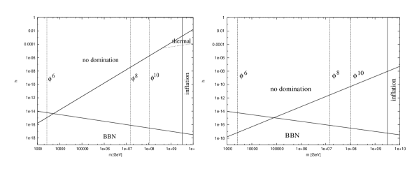
64 Results

Figs. 1 and 2 shows the parameter space for curvaton domination: $f\stackrel{{\scriptstyle>}}{{{}_{\scriptstyle\sim}}}0.5$. In the figure 18 the reheating temperature is arbitrary high, whereas in the figure 19 the gravitino constraint is taken into account. In all parameter space $m_{\phi}\sim 10^{-4}H_{*}$. Models with $V_{\rm NR}\sim\phi^{4+n}/{M_{\rm P}}^{n}$ and $n\leq 2$ are ruled out. For higher values of $n$, the curvaton scenario can be succesfull for curvaton masses in the range $10^{4}{\,\mbox{GeV}}\stackrel{{\scriptstyle<}}{{{}_{\scriptstyle\sim}}}m_{\phi}\stackrel{{\scriptstyle<}}{{{}_{\scriptstyle\sim}}}10^{9}{\,\mbox{GeV}}$. Couplings have to be small $h\stackrel{{\scriptstyle<}}{{{}_{\scriptstyle\sim}}}10^{-6}$, even $h\stackrel{{\scriptstyle<}}{{{}_{\scriptstyle\sim}}}10^{-10}$ if the gravitino constraint is taken into account. Thermal effects can be neglected for such small couplings.

One can ask whether there are any natural canditates for the curvaton. Moduli and other fields with only Planck suppressed couplings generically decay after big bang nucleosynthesis, thereby spoiling its succesfull predicitions. MSSM flat directions typically have too small masses and too large couplings to play the rôle of the curvaton. Better curvaton candidates are the right-handed sneutrino and the Peccei-Quinn axion, which can have large masses and small couplings. In all cases though, considerable tuning of parameters is needed.

*$D$-Branes and Unitarity of Noncommutative Field Theories Alessandro Torrielli

Since the seminal work of Seiberg and Wittensw it was realized that open strings in the presence of an antisymmetric constant background are effectively described at low energy by certain noncommutative field theories, identified by a precise set of Feynman rulesf . The derivation by Seiberg and Witten was originally made for magnetic backgrounds only, corresponding to space-space noncommutativity. For electric backgrounds it is well known that problems are present when the electric field approaches a critical value $E_{cr}$, beyond which the string develops a classical instabilityb ; bp ; sst1 : tachyonic masses appear in the spectrum both for neutral (which is the case we will consider here) and charged open strings, connected with the vanishing of the effective tension and an uncontrolled growth of the oscillation amplitude of the modes in the direction parallel to the field. For purely charged strings this phenomenon (which has no analog in particle field theory) coexists with the quantum instability due to pair production which is the analog of the Schwinger phenomenon in particle electrodynamics. When one tries to perform the Seiberg-Witten zero-slope limit to noncommutative field theories one reaches a point in which the ratio between the electric field and its critical value becomes greater than one, and the string enters the region of instability. We will show that precisely at this point a flip-mechanism produces the appearance of the tachyonic branch cut due to the closed string sector in the non-planar diagrams, which is responsible for the lack of unitarity of the limit amplitude. We relate the breaking of perturbative unitarity of these space-time noncommutative theories with the fact that they coincide with those obtained by conveying string theory in an unstable vacuum. This vacuum is likely to decay in the full string theory to a suitable configuration of branes.

We take as action for a bosonic open string attached to a D-brane lying in the first $p+1$ dimensions with an antisymmetric constant background on its worldvolume the following

$$S=\frac{1}{4\pi{\alpha}^{\prime}}\int_{C_{2}}d^{2}z\,(g_{ij}{\partial}_{a}X^{i}{\partial}^{a}X^{j}-2i\pi{\alpha}^{\prime}B_{ij}{\epsilon}^{ab}{\partial}_{a}X^{i}{\partial}_{b}X^{j}).$$ (2)

At one loop the string world-sheet is the cylinder $C_{2}=\{0\leq\Re w\leq 1,w\equiv w+2i\tau$}.

If one sets $w=x+iy$, the relevant propagator on the boundary of the cilinder ($x=0,1$) can be written asad

$$G(y,y^{\prime})={{1}\over{2}}{\alpha}^{\prime}g^{-1}\log q-2{\alpha}^{\prime}G^{-1}\log\Big{[}{{q^{{1}\over{4}}}\over{D(\tau)}}\,{\vartheta_{4}}({{|y-y^{\prime}|}\over{2\tau}},{{i}\over{\tau}})\Big{]},\,\,\,x\neq x^{\prime},$$ (3)

$$G(y,y^{\prime})={{\pm i\theta}\over{2}}{\epsilon}_{\perp}(y-y^{\prime})-2{\alpha}^{\prime}G^{-1}\log\Big{[}{{1}\over{D(\tau)}}{\vartheta_{1}}({{|y-y^{\prime}|}\over{2\tau}},{{i}\over{\tau}})\Big{]},\,\,\,x=x^{\prime},$$ (4)

where $q=e^{-{{\pi}\over{\tau}}}$, $\pm$ correspond to $x=1$ and $x=0$ respectively, and ${\epsilon}_{\perp}(y)=sign(y)-{{y}\over{\tau}}$. The open string parameters are as in sw . With this propagator and the suitable modular measure, the non-planar two-point function can be written as follows:

$$A_{1.2} = {\cal{N}}{G_{s}}^{2}\,2^{{3d}\over 2}{\pi}^{{{3d}\over{2}}-2}{\alpha^{\prime}}^{{{d}\over{2}}-3}\int_{0}^{\infty}dt\,t^{1-{{d}\over{2}}}\,{\Big{[}\eta({{it}\over{2\pi{\alpha^{\prime}}}})\Big{]}}^{2-d}\times$$ (5)

$$\,e^{-{{{\pi}^{2}}{\alpha^{\prime}}^{2}\over{t}}kg^{-1}k}\int_{0}^{1}d\nu{\Bigg{[}{{e^{-{{{\pi}^{2}}{\alpha^{\prime}}\over{2t}}}{\vartheta_{4}}(\nu,{{2\pi i{\alpha^{\prime}}}\over{t}})}\over{{{2\pi{\alpha^{\prime}}}\over{t}}{[\eta({2\pi i{\alpha^{\prime}}\over{t}})]}^{3}}}\Bigg{]}}^{-2{\alpha^{\prime}}kG^{-1}k}.$$

Here ${\cal{N}}$ is the normalization constant, $d=p+1$, $G_{s}$ is the open string coupling constant. We have omitted the traces of the Chan-Paton matrices.

This is a form suitable for the field theory limit. We perform the zero-slope limit of Seiberg and Witten, which consists in sending ${\alpha}^{\prime}\to 0$ keeping $\theta$ and $G$ fixed (in this case we will keep $t$ and $\nu$ fixed as well). This can be done setting ${\alpha}^{\prime}\sim{\epsilon}^{1\over 2}$ and the closed string metric $g\sim\epsilon$, and then sending $\epsilon\to 0$ sw . One obtains ad

$$A_{1.2}^{lim}={\cal{N}}2^{{3d}\over 2}{\pi}^{{{3d}\over{2}}-2}{g_{f}}^{2}\int_{0}^{\infty}dtt^{1-{{d}\over{2}}}e^{-m^{2}t\,+\,k\theta G\theta k/4t}\int_{0}^{1}d\nu e^{-t\,\nu(1-\nu)\,kG^{-1}k}.$$ (6)

This reproduces the expression for the two-point function in the noncommutative $\phi^{3}$ theorydn ; s ; tesi with coupling constant $g_{f}=G_{s}\,{{\alpha}^{\prime}}^{{{d-6}\over{4}}}$. We choose now $d=2$. This case is peculiar, since the tachyon mass ${m^{2}}={{2-d}\over{24{\alpha}^{\prime}}}$ goes to zero. In two dimensions the background is an electric one and noncommutativity is necessarily space-time.

In order to interpret the field theory analysis, one continues the expression (5) in the complex variable $k^{2}=kG^{-1}k$. It has a branch cut driven by the small-$t$ (closed-channel) behavior

$$\exp\Big{(}-k^{2}\,{{{\pi}^{2}{{\alpha^{\prime}}^{2}\,[1-{(E/E_{cr})}^{2}]}}\over{t}}\Big{)}.$$ (7)

The field-theory limit retains in turn another branch cut $Re[S]=Re[-k^{2}]>0$ from the large-$t$ behaviour

$$\exp\Big{(}-k^{2}\,t\,\nu(1-\nu)\Big{)}.$$ (8)

$E_{cr}={{g}\over{2\pi{\alpha^{\prime}}}}$ is the critical value of the electric field. The small-$t$ cut is on the physical side $Re[S]=Re[-k^{2}]>0$. But we see that it is driven by a quantity which changes sign if the electric field overcomes its critical value, that is when the string enters the classical instability region. This is exactly what the Seiberg-Witten limit produces, since it scales ${(E/E_{cr})}^{2}\sim{(\alpha^{\prime}/g)}^{2}\sim 1/\epsilon$. In the field theory limit the branch cut flips to the unphysical sidemio , and in fact the amplitude (6) for $m^{2}=0$ has two branch cuts, one of which is physical, the other one tachyonic, coalescing at the origin. By treating $m^{2}$ as a free parameter independent of $d$ and by taking it positive, one can see the shift of (7) to a cut starting from $S>4m^{2}$ which gives the physical pair-production cut, and a closed branch cut starting at $S>4m^{2}/[1-{({{E}/{E_{cr}}})}^{2}]$, which flips in the limit.

*Spinorial Cohomology and Supersymmetry Dimitrios Tsimpis

String theory reduces at low energies to ordinary field theory supplemented by an infinite tower of higher-order curvature (derivative) corrections organised in a double-series expansion in $\alpha^{\prime}$ and $g_{string}$. These corrections can in principle be derived by string-theoretical perturbative methods, but in certain cases supersymmetry alone is restrictive enough to detrmine them.

The question is more sharply posed in the case of M-theory (see duff for a review) whose low-energy effective field-theory limit is captured by ordinary eleven-dimensional supergravity Cremmer:1978km . In order to gain insight into the nature of M-theory, one needs to go beyond this limiting approximation; for example, by including supersymmetric higher-order curvature corrections. In the absence of an underlying perturbative analogue of string theory such corrections cannot be found systematically, even in principle, but one might hope that supersymmetry would be sufficient to determine at least the first-order correction.

Higher-order corrections have far-reaching implications to a variety of physical problems at the heart of our understanding of M-theory: they can be used to derive modifications to macroscopic black hole properties such as the entropy-area formula and to test duality conjectures, like the AdS/CFT correspondence, beyond the leading-order approximation; they may give a mechanism for moduli stabilisation and they may provide a way to bypass no-go theorems concerning dS vacua. However, even the first such deformation –corresponding to canonical mass dimension six operators ($R^{4}$)– has proven notoriously difficult to determine.

The construction of the complete $R^{4}$ terms in type II string theory or in M-theory remains an open problem, see Peeters:2000qj for a review and further references. A recent attempt was made in deHaro:2002vk to construct an $R^{4}$ action in type IIB based on a chiral measure in on-shell IIB superspace, but it was subsequently observed that such a measure does not exist bh . A completely different approach was taken by the authors of Peeters:2000qj who used partial results from type II string theory and attempted to lift them to eleven dimensions, but this proved to be too difficult to carry out completely.

Recently-developed techniques relating to the study of supersymmetric theories, which go under the name of spinorial cohomology, offer perhaps the most promising and comprehensive approach to tackling these long-standing issues. Spinorial cohomology, which is the subject of this brief review, was introduced in cnta and was further elaborated in cntc . It provides a powerful and systematic way of organising the field content and the possible deformations of supersymmetric theories, as well as explicitly determining higher-order curvature corrections. Pure-spinor cohomology paul , which was recently used by Berkovits in a covariant approach to string theory berk ; Berkovits:2002uc , has been shown to be isomorphic to the concept of spinorial-cohomology with unrestricted coefficients h ; ht .

Spinorial-cohomology has already found applications in a variety of contexts; in studies of ten-dimensional maximally-supersymmetric Yang-Mills theories cnta ; cntb ; cntd , eleven-dimensional supergravity cntc ; ht ; cgnt , and the world-volume effective theory of the M2 brane hklt . In cntb ; hklt the first-order curvature correction to $D=10$, $N=1$ SYM and to the M2-brane action respectively, was given explicitly. In ht a method was outlined which makes it possible to read off the first deformation of eleven-dimensional supergravity from the five-brane anomaly-cancelling term. Moreover, it was argued that the supersymmetric completion of this term is the unique anomaly-cancelling invariant at this dimension which is at least quartic in the fields.

In order to give a geometrical definition of spinorial cohomology (see ht for a more detailed discussion), we will suppose that we have the usual machinery of supergravity, i.e. Lorentzian structure group, connection, torsion and curvature. In particular we suppose that the tangent bundle is a direct sum of the odd and even bundles. The space of forms admits a natural bigrading according to the degrees of the forms and their Grassmann character. The space of forms with $p$ even and $q$ odd components is denoted by $\Omega^{p,q}$. The exterior derivative $d$ maps $\Omega^{p,q}$ to $\Omega^{p+1,q}+\Omega^{p,q+1}+\Omega^{p-1,q+2}+\Omega^{p+2,q-1}$. Following Bonora:mt we split $d$ into its various components with respect to the bigrading

$$d=d_{0}+d_{1}+\tau_{0}+\tau_{1}~{},$$ (9)

where $d_{0}(d_{1})$ is the even (odd) derivative with bidegrees $(1,0)$ and $(0,1)$ respectively, while $\tau_{0}$ and $\tau_{1}$ have bidegrees $(-1,2)$ and $(2,-1)$. These two latter operators are purely algebraic and involve the dimension-zero and dimension-three-halves components of the torsion tensor respectively. The fact that $d^{2}=0$ implies in particular that $\tau_{0}^{2}=0$. We can therefore consider the cohomology of $\tau_{0}$ and set

$$H^{p,q}_{\tau}=\{\omega\in\Omega^{p,q}|\tau_{0}\omega=0\ {\rm mod}\ \omega=\tau_{0}\lambda,\lambda\in\Omega^{p+1,q-2}\}~{}.$$ (10)

We can now define a spinorial derivative $d_{F}$ which will act on elements of $H^{p,q}_{\tau}$. If $\omega\in[\omega]\in H^{p,q}_{\tau}$ we set

$$d_{F}[\omega]:=[d_{1}\omega]~{}.$$ (11)

It is easy to check that this is well-defined, i.e. $d_{1}\omega$ is $\tau_{0}$-closed, and $d_{F}[\omega]$ is independent of the choice of representative. Furthermore it is simple to check that $d_{F}^{2}=0$. This means that we can define the spinorial cohomology groups

$$H^{p,q}_{F}:=H^{p,q}(d_{F}|H_{\tau})~{},$$ (12)

in the obvious fashion.

To illustrate the meaning of the cohomology groups let us now turn to $D=10$, $N=1$ SYM. The two lowest-dimensional components of the Bianchi identity are

$$d_{1}F_{0,2}+\tau_{0}F_{1,1} = 0$$ (13)

$$d_{1}F_{1,1}+\tau_{0}F_{2,0} = 0~{}.$$ (14)

The ordinary (undeformed) theory is obtained by setting $[F_{0,2}]=0$ and this is equivalent to specifying an element of $H^{0,1}_{F}$. Hence we can set $F_{0,2}=0$ in which case $F_{1,1}$ determines an element of $H^{1,1}_{F}$. One can easily see that this cohomology group is a spinor superfield $\lambda^{\alpha}$ satisfying the constraint $D_{\alpha}\lambda^{\beta}=(\gamma^{ab})_{\alpha}{}^{\beta}F_{ab}$, i.e. it is the on-shell field strength supermultiplet.

If we relax the ordinary constrain $F_{\alpha\beta}=0$ by introducing a current $J_{\alpha\beta}$ on the right-hand side, then the latter must be spinorially closed by virtue of the Bianchi identity. On the other hand, if it is trivial, the connection can be redefined to regain the original equations of motion. This implies that $H^{0,2}_{F}$ describes the currents of the theory (which are in one-to-one correspondence with the anti-fields). If we are interested in looking at deformations of the theory, we need to consider the same cohomology group but with the coefficients restricted to be tensorial functions of the field strength superfield $\lambda$ and its derivatives. We denote this group by $H^{0,2}_{F}(phys)$. The two groups are quite different; the former is dual to the physical fields while the latter describes a composite multiplet in the theory. The group $H^{0,2}_{F}(phys)$ has been explicitly computed in cnta for the nonabelian SYM at order $\alpha^{\prime 2}$ to give the most general supersymmetric action at this order cntb . It has also been computed for the abelian SYM at order $\alpha^{\prime 3}$ to prove rigorously the absence of any supersymmetric deformation cntd .

Eleven-dimensional supergravity can also be understood in terms of spinorial cohomolgy groups cntc ; ht . Apart from a purely geometrical formulation in terms of the supertorsion hw , the theory admits a formulation in terms of a closed four-form in superspace. From this point of view, physical fields are elements of $H^{0,3}_{F}$, while deformations are parametrized by the $H^{0,4}_{F}(phys)$ spinorial-cohomology group cntc ; ht .

One can also give a description in terms of a ‘dual’ super four-form obeying a deformed Bianchi identity Duff:1995wd ; cgnn

$$dG_{7}=\frac{G}{2}_{4}^{2}+\beta X_{8}~{},$$ (15)

where $\beta$ is a parameter of dimension $\ell^{6}$ and $X_{8}=\operatorname{Tr}(R^{4})-{1\over 4}(\operatorname{Tr}(R^{2}))^{2}$. This equation uses imput from M-theory, namely the five-brane anomaly cancellation condition, and it can be used to read off the deformation consistent with $X_{8}$. One can then make contact with the four-form formulation by solving the BI’s up to dimension -1 ht .

The solution of the supertorsion Bianchi identities of eleven-dimensional supergravity will be presented in cgnt , completing the work initiated in cgnn . Moreover, provided a nontrivial element of the spinorial-cohomology group $H^{0,4}_{F}(phys)$ has been determined through the procedure described above, the information can be fed in the results of ht ; cgnt to give the explicit expression of the deformed equations of motion –and therefore the first-order ($R^{4}$) correction to the Lagrangian– of eleven-dimensional supergravity. This procedure, albeit tedious, is straightforward and can be carried out in practice.

References

- (1) S. Dimopoulos, S. Raby and F. Wilczek, Phys. Rev. D 24 (1981) 1681; L. E. Ibañez and G. G. Ross, Phys. Lett. B 105 (1981) 439; M. B. Einhorn and D. R. Jones, Nucl. Phys. B 196 (1982) 475; W. J. Marciano and G. Senjanović, Phys. Rev. D 25 (1982) 3092.
- (2) K. Inoue, A. Kakuto, H. Komatsu and S. Takeshita, Prog. Theor. Phys. 68 (1982) 927 [Erratum-ibid. 70 (1983) 330]; L. Alvarez-Gaume, J. Polchinski and M. B. Wise, Nucl. Phys. B 221 (1983) 495.
- (3) G. Lazarides, Q. Shafi and C. Wetterich, Nucl. Phys. B 181 (1981) 287.
- (4) K. S. Babu and R. N. Mohapatra, Phys. Rev. Lett. 70 (1993) 2845 [arXiv:hep-ph/9209215].
- (5) C. S. Aulakh, K. Benakli and G. Senjanović, Phys. Rev. Lett. 79 (1997) 2188 [arXiv:hep-ph/9703434]; C. S. Aulakh, A. Melfo and G. Senjanović, Phys. Rev. D 57 (1998) 4174 [arXiv:hep-ph/9707256]; C. S. Aulakh, A. Melfo, A. Rašin and G. Senjanović, Phys. Lett. B 459 (1999) 557 [arXiv:hep-ph/9902409].
- (6) J. Hisano, H. Murayama and T. Yanagida, Nucl. Phys. B 402 (1993) 46 [arXiv:hep-ph/9207279]; T. Goto and T. Nihei, Phys. Rev. D 59 (1999) 115009 [arXiv:hep-ph/9808255]; H. Murayama and A. Pierce, Phys. Rev. D 65 (2002) 055009 [arXiv:hep-ph/0108104].
- (7) B. Bajc, P. F. Perez and G. Senjanović, Phys. Rev. D 66 (2002) 075005 [arXiv:hep-ph/0204311] and arXiv:hep-ph/0210374.
- (8) A. Masiero, D. V. Nanopoulos, K. Tamvakis and T. Yanagida, Phys. Lett. B 115 (1982) 380.
- (9) S. Dimopoulos and F. Wilczek, Print-81-0600 (SANTA BARBARA); K. S. Babu and S. M. Barr, Phys. Rev. D 48 (1993) 5354 [arXiv:hep-ph/9306242] and Phys. Rev. D 65 (2002) 095009 [arXiv:hep-ph/0201130].
- (10) see for example Z. Berezhiani, C. Csaki and L. Randall, Nucl. Phys. B 444 (1995) 61 [arXiv:hep-ph/9501336], and references therein.
- (11) R. Barbieri, G. R. Dvali and A. Strumia, Phys. Lett. B 333 (1994) 79 [arXiv:hep-ph/9404278]; S. M. Barr, Phys. Rev. D 55 (1997) 6775 [arXiv:hep-ph/9607359]; E. Witten, arXiv:hep-ph/0201018; M. Dine, Y. Nir and Y. Shadmi, Phys. Rev. D 66 (2002) 115001 [arXiv:hep-ph/0206268].
- (12) C. Bachas, C. Fabre and T. Yanagida, Phys. Lett. B 370 (1996) 49 [arXiv:hep-th/9510094]; J. L. Chkareuli and I. G. Gogoladze, Phys. Rev. D 58 (1998) 055011 [arXiv:hep-ph/9803335].
- (13) V. V. Dixit and M. Sher, Phys. Rev. D 40 (1989) 3765.
- (14) G. R. Dvali, Phys. Lett. B 287 (1992) 101; P. Nath, Phys. Rev. Lett. 76 (1996) 2218 [arXiv:hep-ph/9512415]; P. Nath, Phys. Lett. B 381 (1996) 147 [arXiv:hep-ph/9602337]; V. Lucas and S. Raby, Phys. Rev. D 55 (1997) 6986 [arXiv:hep-ph/9610293]; Z. Berezhiani, Z. Tavartkiladze and M. Vysotsky, arXiv:hep-ph/9809301; K. Turzynski, JHEP 0210 (2002) 044 [arXiv:hep-ph/0110282]; D. Emmanuel-Costa and S. Wiesenfeldt, Nucl. Phys. B 661 (2003) 62 [arXiv:hep-ph/0302272].
- (15) T. Friedmann and E. Witten, arXiv:hep-th/0211269; I. R. Klebanov and E. Witten, Nucl. Phys. B 664 (2003) 3 [arXiv:hep-th/0304079].
- (16) R. N. Mohapatra, Phys. Rev. Lett. 43 (1979) 893.
- (17) S. Nandi, A. Stern and E. C. G. Sudarshan, Phys. Lett. B 113 (1982) 165; V. S. Berezinsky and A. Y. Smirnov, Phys. Lett. B 140 (1984) 49.
- (18) C. S. Aulakh, B. Bajc, A. Melfo, A. Rašin and G. Senjanović, Nucl. Phys. B 597 (2001) 89 [arXiv:hep-ph/0004031].
- (19) V. A. Rubakov, Nucl. Phys. B 203 (1982) 311; C. G. Callan, Phys. Rev. D 25 (1982) 2141 and Phys. Rev. D 26 (1982) 2058.
- (20) K. Freese, M. S. Turner and D. N. Schramm, Phys. Rev. Lett. 51 (1983) 1625.
- (21) G. Giacomelli and L. Patrizii, arXiv:hep-ex/0302011.
- (22) A. Melfo and G. Senjanović, Phys. Rev. D 68 (2003) 035013 [arXiv:hep-ph/0302216], and references therein.
- (23) R. Barbieri and L. J. Hall, Phys. Lett. B 338 (1994) 212 [arXiv:hep-ph/9408406].
- (24) I. Masina and C. Savoy, arXiv:hep-ph/0309067.
- (25) K. S. Babu and R. N. Mohapatra, Phys. Lett. B 518 (2001) 269 [arXiv:hep-ph/0108089].
- (26) F. Wilczek and A. Zee, Phys. Rev. D 25 (1982) 553.
- (27) see for example C. H. Albright and S. M. Barr, Phys. Rev. Lett. 85 (2000) 244 [arXiv:hep-ph/0002155]; K. S. Babu, J. C. Pati and F. Wilczek, Nucl. Phys. B 566 (2000) 33 [arXiv:hep-ph/9812538]; T. Blažek, S. Raby and K. Tobe, Phys. Rev. D 60 (1999) 113001 [arXiv:hep-ph/9903340].
- (28) M. C. Chen and K. T. Mahanthappa, arXiv:hep-ph/0305088.
- (29) R. N. Mohapatra, Phys. Rev. D 34 (1986) 3457.
- (30) T. E. Clark, T. K. Kuo and N. Nakagawa, Phys. Lett. B 115 (1982) 26; D. G. Lee, Phys. Rev. D 49 (1994) 1417.
- (31) C. S. Aulakh and R. N. Mohapatra, Phys. Rev. D 28 (1983) 217.
- (32) C. S. Aulakh, B. Bajc, A. Melfo, G. Senjanović and F. Vissani, arXiv:hep-ph/0306242.
- (33) M. Gell-Mann, P. Ramond and R. Slansky, proceedings of the Supergravity Stony Brook Workshop, New York, 1979, eds. P. Van Niewenhuizen and D. Freeman (North-Holland, Amsterdam); T. Yanagida, proceedings of the Workshop on Unified Theories and Baryon Number in the Universe, Tsukuba, Japan 1979 (edited by A. Sawada and A. Sugamoto, KEK Report No. 79-18, Tsukuba); R. N. Mohapatra and G. Senjanović, Phys. Rev. Lett. 44 (1980) 912.
- (34) M. Magg and C. Wetterich, Phys. Lett. B 94 (1980) 61; R. N. Mohapatra and G. Senjanović, Phys. Rev. D 23 (1981) 165.
- (35) D. G. Lee and R. N. Mohapatra, Phys. Rev. D 51 (1995) 1353 [arXiv:hep-ph/9406328].
- (36) K. Matsuda, Y. Koide, T. Fukuyama and H. Nishiura, Phys. Rev. D 65 (2002) 033008 [Erratum-ibid. D 65 (2002) 079904] [arXiv:hep-ph/0108202]; T. Fukuyama and N. Okada, JHEP 0211 (2002) 011 [arXiv:hep-ph/0205066].
- (37) B. Bajc, G. Senjanović and F. Vissani, arXiv:hep-ph/0110310.
- (38) B. Bajc, G. Senjanović and F. Vissani, Phys. Rev. Lett. 90 (2003) 051802 [arXiv:hep-ph/0210207].
- (39) H. S. Goh, R. N. Mohapatra and S. P. Ng, Phys. Lett. B 570 (2003) 215 [arXiv:hep-ph/0303055].
- (40) H. S. Goh, R. N. Mohapatra and S. P. Ng, arXiv:hep-ph/0308197.
- (41) B. Brahmachari and R. N. Mohapatra, Phys. Rev. D 58 (1998) 015001 [arXiv:hep-ph/9710371].
- (42) S. F. King, arXiv:hep-ph/0310204.
- (43) D. G. Lee and R. N. Mohapatra, Phys. Lett. B 324 (1994) 376 [arXiv:hep-ph/9310371].
- (1) M. Pavšič, The Landscape of Theoretical Physics: A Global View. From Point Particles to the Brane World and Beyond, in Search of a Unifying Principle, Kluwer, Dordrecht, 2001.
- (2) K. Bardakci, Nucl. Phys. B271 (1986) 561.
- (3) M. Pavšič, Found. Phys. 26 (1996) 159; Nuov. Cim. A 110 (1997) 369.
- (4) V. Moncrief and C. Teitelboim, Phys. Rev. D 6 (1972) 966.
- (5) L. Smolin, Phys. Rev. D 62 (2000) 086001.
- (6) C. Castro, J. Chaos Solitons Fractals 11 (2000) 1721, hep-th/9912113; J. Chaos, Solitons and Fractals 12 (2001) 1585, physics/0011040.
- (7) W.M. Pezzaglia Jr, A Clifford Algebra Multivector Reformulation of Field Theory, Dissertation, University of California, Davis, 1983; “Classification of Multivector Theories and Modification o f the Postulates of Physics”, gr-qc/9306006; “Polydimensional Relativity, a Classical Generalization of the Automorphism Invariance Principle”, gr-qc/9608052; “Physical Applications of a Generalized Clifford Calculus: Papapetrou Equations and Metamorphic Curvature”, gr-qc/9710027.
- (8) M. Pavšič, Found. Phys. 31, 1185 (2001) 1185, hep-th/0011216; Found. Phys. 33 (2003) 1277, gr-qc/0211085; Class. Quant. Grav. 20 (2003) 2697, gr-qc/0111092; C. Castro and M. Pavšič, Phys. Lett. B 539 (2002) 133, hep-th/0110079.
- (9) D. Hestenes, Space-Time Algebra, Gordon and Breach, New York, 1966; D. Hestenes Clifford Algebra to Geometric Calculus D. Reidel, Dordrecht, 1984.
- (10) N. S. Mankoč Borštnik and H. B. Nielsen, J. Math. Phys. 43 (2002) 5782, hep-th/0111257; J. Math. Phys. 44 (2003) 4817, hep-th/0303224.
- (11) B.S. DeWitt, The Quantization of Geometry, in: L. Witten, Gravitation: An Introduction to Current Research, Wiley, New York, 1962.
- (12) C. Rovelli, Classical and Quantum Gravity 8 (1991) 297; 8 (1991) 317.
- (1) G. Mangano, G. Miele, S. Pastor, and M. Peloso, Phys. Lett. B534, 8 (2002).
- (2) C.L. Bennett et al. (WMAP Coll.), Astrophys. J. Suppl. 148, 1 (2003).
- (3) P. Crotty, J. Lesgourgues, and S. Pastor, Phys. Rev. D67, 123005 (2003).
- (4) E. Pierpaoli, Mon. Not. Roy. Astron. Soc. 342, L63 (2003).
- (5) A. Cuoco et al. ., astro-ph/0307213.
- (6) R.E. Lopez and M.S. Turner, Phys. Rev. D59, 103502 (1999).
- (7) S. Esposito, G. Mangano, G. Miele and O. Pisanti, Nucl. Phys. B568, 421 (2000).
- (8) L.M. Krauss and P. Romanelli, Astrophys. J. 358, 47 (1990); P.J. Kernan and L.M. Krauss, Phys. Rev. Lett. 72, 3309 (1994).
- (9) G. Fiorentini, E. Lisi, S. Sarkar, and F.L. Villante, Phys. Rev. D58, 063506 (1998).
- (10) S. Burles, K.M. Nollett, and M.S. Turner, Astrophys. J. 552, L1 (2001).
- (11) A. Coc, E. Vangioni-Flam, and M. Cassé, astro-ph/0002248; astro-ph/0009297; astro-ph/0101286.
- (12) C. Angulo et al. , Nucl. Phys. A656 (1999) 3. NACRE web site http://pntpm.ulb.ac.be/nacre.htm
- (13) LUNA Collaboration, Nucl. Phys. A706 (2002) 203.
- (14) B.D. Fields, and S. Sarkar, in Review of Particle Properties, Phys. Rev. D66, 010001 (2002).
- (15) D. Kirkman, D. Tytler, N. Suzuki, J.M. O’Meara, and D. Lubin, astro-ph/0302006.
- (16) A.D. Dolgov, S.H. Hansen, S. Pastor, S.T. Petcov, G.G. Raffelt, and D.V. Semikoz, Nucl. Phys. B362, 363 (2002).
- (17) V.M. Lobashev et al. (Troisk Coll.), Phys. Lett. B460, 227 (1999); C. Weinheimer et al. (Mainz Coll.), Phys. Lett. B460, 219 (1999).
- (18) A. Osipowicz et al. , hep-ph/0109033.
- (19) C. Arnaboldi et al. (CUORE Coll.), hep-ex/0212053.
- (20) H.V. Klapdor-Kleingrothaus (GENIUS Coll.), hep-ph/9910205.
- (21) W. Hu, D.J. Eisenstein, and M. Tegmark, Phys. Rev. Lett. 80, 5255 (1998).
- (22) D.N. Spergel et al. , Astrophys. J. Suppl. 148, 175 (2003).
- (23) O. Elgaroy and O. Lahav, JCAP 0304, 004 (2003).
- (24) S. Hannestad, JCAP 0305, 004 (2003).
- (25) J. Peacock et al. , Nature 410, 169 (2001).
- (1) Particle Data Group, K. Hagiwara et al., Phys. Rev. D 66, 010001 (2002).
- (2) M.C. Gonzales-Garcia and Y. Nir, Rev. Mod. Phys. 75, 345 (2003) [arXiv:hep-ph/0202058].
- (3) C.D. Froggatt and H.B. Nielsen, These Proceedings.
-
(4)
N. Cabibbo, L. Maiani, G. Parisi and R. Petronzio, Nucl. Phys. B
158, 295 (1979);
M. Lindner, M. Sher and H.W. Zaglauer, Phys. Lett. B 228, 139 (1989);
M. Sher, Phys. Rep. 179, 273 (1989). - (5) M. Lindner, Z. Phys. C 31, 295 (1986).
- (6) D.L. Bennett, C.D. Froggatt and H.B. Nielsen, Proceedings of the 27th International Conference on High Energy Physics, p. 557, ed. P. Bussey and I. Knowles (IOP Publishing Ltd, 1995); Perspectives in Particle Physics ’94, p. 255, ed. D. Klabuc̆ar, I. Picek and D. Tadić (World Scientific, 1995) [arXiv:hep-ph/9504294].
(7)
S.W. Hawking, Phys. Rev. D 37, 904 (1988);
S. Coleman, Nucl. Phys. B 307, 867 (1988); Nucl. Phys. B 310, 643 (1988);
T. Banks, Nucl. Phys. 309, 493 (1988). - (8) C.D. Froggatt and H.B. Nielsen, Phys. Lett. B 368, 96 (1996) [arXiv:hep-ph/9511371].
- (9) J.A. Casas, J.R. Espinosa and M. Quiros Phys. Lett. B 342, 171 (1995) [arXiv:hep-ph/9409458].
- (10) C.D. Froggatt, H.B. Nielsen and Y. Takanishi, Phys. Rev. D 64, 113014 (2001) [arXiv:hep-ph/0104161].
- (11) C.D. Froggatt and H.B. Nielsen, arXiv:hep-ph/0308144.
- (12) H. Fritzsch, Phys. Lett. B70, 436 (1977).
- (13) P. Ramond, R.G. Roberts and G.G. Ross, Nucl. Phys. B 406, 19 (1993) [arXiv:hep-ph/9303320].
- (14) J.L. Chkareuli and C.D. Froggatt, Phys. Lett. B B50, 158 (1999) [arXiv:hep-ph/9812499].
- (15) K. Matsuda, T. Fukuyama and H. Nishiura, Phys. Rev. D 60, 013006 (1999) [arXiv:hep-ph/9902385].
- (16) J.L. Chkareuli, C.D. Froggatt and H.B. Nielsen, Nucl. Phys. B 626, 307 (2002) [arXiv:hep-ph/0109156].
- (17) S.F. King, and G.G. Ross, Phys. Lett. B 574, 239 (2003) [arXiv:hep-ph/0307190].
- (18) C.D. Froggatt, H.B. Nielsen and D.J. Smith, Phys. Lett. B 385, 150 (1996) [arXiv:hep-ph/9607250]; C.D. Froggatt, M. Gibson, H.B. Nielsen and D.J. Smith, Int. J. Mod. Phys. A 13 5037 (1998) [arXiv:hep-ph/9706212].
- (19) C.D. Froggatt, H.B. Nielsen and Y. Takanishi, Nucl. Phys. B 631, 285 (2002) [arXiv:hep-ph/0201152]; H.B. Nielsen and Y. Takanishi, Phys. Lett. B 543, 249 (2002) [arXiv:hep-ph/0205180].
- (20) C.D. Froggatt and H.B. Nielsen, Nucl. Phys. B 147, 277 (1979).
- (21) F.S. Ling and P. Ramond, Phys. Rev. D 67, 115010 (2003) [arXiv:hep-ph/0302264].
(22)
M. Gell-Mann, P. Ramond and R. Slansky in Supergravity,
p. 315; Eds. P. van Nieuwenhuizen and D. Z. Freedman (North
Holland, New York, 1980);
T. Yanagida, Proc. of the Workshop on Unified Theory and Baryon Number in the Universe 1979, p. 95; Eds. A. Sawada and H. Sugawara (KEK, Tsukuba-Gu, Ibaraki-ken, Japan, 1979);
R.N. Mohapatra and G. Senjanovic, Phys. Rev. Lett. 44 (1980). - (23) C.D. Froggatt, H.B. Nielsen and D. Smith, Phys. Rev. D 65, 095007 (2002) [arXiv:hep-ph/0108262].
- (1) G. T. Horowitz, (1996), gr-qc/9604051; C. Rovelli, Living Rev. Rel. 1, 1 (1998), gr-qc/9710008; Notes for a brief history of quantum gravity, in 9th Marcel Grossmann Meeting On Recent Developments In Theoretical And Experimental General Relativity, Gravitation And Relativistic Field Theories, 2000, arXiv:gr-qc/0006061.
- (2) S. Carlip, Rept. Prog. Phys. 64, 885 (2001), arXiv:gr-qc/0108040; L. Smolin, (2003), hep-th/0303185.
- (3) K. Eppley and E. Hannah, Found. Phys. 7, 51 (1977).
- (4) T. Banks, Nucl. Phys. Proc. Suppl. 41, 21 (1995), hep-th/9412131.
- (5) G. ’t Hooft and M. J. G. Veltman, Annales Poincare Phys. Theor. A20, 69 (1974).
- (6) D. Grumiller, W. Kummer, and D. V. Vassilevich, Phys. Rept. 369, 327 (2002), hep-th/0204253.
- (7) M. Nakahara, Geometry, Topology and Physics (IOP Publishing, Bristol, 1990).
- (8) A. Sen, Phys. Lett. B119, 89 (1982); A. Ashtekar, Phys. Rev. Lett. 57, 2244 (1986); Phys. Rev. D36, 1587 (1987); C. Rovelli, Class. Quant. Grav. 8, 1613 (1991).
- (9) J. F. Barbero, Phys. Rev. D51, 5507 (1995), gr-qc/9410014; G. Immirzi, Class. Quant. Grav. 14, L177 (1997), gr-qc/9612030; Nucl. Phys. Proc. Suppl. 57, 65 (1997), gr-qc/9701052.
- (10) A. Einstein, Annalen Phys. 49, 769 (1916).
- (11) M. Fierz, Helv. Phys. Acta 29, 128 (1956); P. Jordan, Z. Phys. 157, 112 (1959); C. Brans and R. H. Dicke, Phys. Rev. 124, 925 (1961).
- (12) E. E. Salpeter and H. A. Bethe, Phys. Rev. 84, 1232 (1951); N. Nakanishi, Prog. Theor. Phys. Suppl. 43, 1 (1969); R. Barbieri and E. Remiddi, Nucl. Phys. B141, 413 (1978); W. E. Caswell and G. P. Lepage, Phys. Rev. A18, 810 (1978).
- (13) W. Kummer, Eur. Phys. J. C21, 175 (2001), hep-th/0104123.
- (14) J. A. Dixon and J. C. Taylor, Nucl. Phys. B78, 552 (1974); J. A. Dixon, Nucl. Phys. B99, 420 (1975); H. Kluberg-Stern and J. B. Zuber, Phys. Rev. D12, 467 (1975); W. Konetschny and W. Kummer, Nucl. Phys. B124, 145 (1977); S. D. Joglekar and B. W. Lee, Ann. Phys. 97, 160 (1976).
- (15) J. I. Friedman, H. W. Kendall, and R. E. Taylor, Rev. Mod. Phys. 63, 573 (1991).
- (16) D. J. Gross and F. Wilczek, Phys. Rev. D8, 3633 (1973); Phys. Rev. D9, 980 (1974).
- (17) A. M. Polyakov, Nucl. Phys. B164, 171 (1980); V. S. Dotsenko and S. N. Vergeles, Nucl. Phys. B169, 527 (1980); R. A. Brandt, F. Neri, and M.-a. Sato, Phys. Rev. D24, 879 (1981); J. Frenkel and J. C. Taylor, Nucl. Phys. B246, 231 (1984).
- (18) A. Andrasi, Eur. Phys. J. C18, 601 (2001), hep-th/9912138.
- (19) J. F. Donoghue, Phys. Rev. D50, 3874 (1994), gr-qc/9405057.
- (20) G. W. Gibbons and S. W. Hawking, editors, Euclidean quantum gravity (Singapore: World Scientific, 1993).
- (21) R. Arnowitt, S. Deser, and C. W. Misner, in Gravitation: An Introduction to Current Research, edited by L. Witten, Wiley, New York, 1962.
- (22) C. G. Torre and M. Varadarajan, Class. Quant. Grav. 16, 2651 (1999), hep-th/9811222.
- (23) B. S. DeWitt, Phys. Rev. 160, 1113 (1967); C. W. Misner, Phys. Rev. 186, 1319 (1969).
- (24) K. Kuchař, Phys. Rev. D4, 955 (1971).
- (25) P. Bergmann and A. Komar, in Recent developments in general relativity, Pergamon, New York, 1962; C. Teitelboim, Phys. Lett. B56, 376 (1975); K. Kuchař, in Quantum gravity 2: an Oxford symposium, edited by C. Isham, R. Penrose, and D. Sciama, Clarendon Press, Oxford, 1975.
- (26) J. Polchinski, String theory (Cambridge University Press, 1998), Vol. 1: An Introduction to the Bosonic String; Vol. 2: Superstring Theory and Beyond.
- (27) A. G. Riess et al., Astrophys. J. 560, 49 (2001), astro-ph/0104455; A. G. Riess, The Publications of the Astronomical Society of the Pacific 112, 1284 (2000); Supernova Search Team, A. G. Riess et al., Astron. J. 116, 1009 (1998), astro-ph/9805201; Supernova Cosmology Project, S. Perlmutter et al., Astrophys. J. 517, 565 (1999), arXiv:astro-ph/9812133.
- (28) P. Van Nieuwenhuizen, Phys. Rept. 68, 189 (1981).
- (29) G. Mandal, A. M. Sengupta, and S. R. Wadia, Mod. Phys. Lett. A6, 1685 (1991); S. Elitzur, A. Forge, and E. Rabinovici, Nucl. Phys. B359, 581 (1991); E. Witten, Phys. Rev. D44, 314 (1991); R. Dijkgraaf, H. Verlinde, and E. Verlinde, Nucl. Phys. B371, 269 (1992); C. G. Callan, Jr., S. B. Giddings, J. A. Harvey, and A. Strominger, Phys. Rev. D45, 1005 (1992), hep-th/9111056.
- (30) B. M. Barbashov, V. V. Nesterenko, and A. M. Chervyakov, Teor. Mat. Fiz. 40, 15 (1979); J. Phys. A13, 301 (1979); Theor. Math. Phys. 40, 572 (1979); E. D’Hoker and R. Jackiw, Phys. Rev. D26, 3517 (1982); C. Teitelboim, Phys. Lett. B126, 41 (1983); E. D’Hoker, D. Freedman, and R. Jackiw, Phys. Rev. D28, 2583 (1983); E. D’Hoker and R. Jackiw, Phys. Rev. Lett. 50, 1719 (1983); R. Jackiw, (1995), hep-th/9501016.
- (31) N. Ikeda and K. I. Izawa, Prog. Theor. Phys. 90, 237–246 (1993), hep-th/9304012; N. Ikeda, Ann. Phys. 235 435–464 (1994), hep-th/9312059; P. Schaller and T. Strobl, Mod. Phys. Lett. A9 3129–3136 (1994), hep-th/9405110.
- (32) W. Kummer and D. J. Schwarz, Nucl. Phys. B382, 171 (1992); F. Haider and W. Kummer, Int. J. Mod. Phys. A9, 207 (1994); W. Kummer, H. Liebl, and D. V. Vassilevich, Nucl. Phys. B493, 491 (1997), gr-qc/9612012; Nucl. Phys. B544, 403 (1999), hep-th/9809168; D. Grumiller, Quantum dilaton gravity in two dimensions with matter, PhD thesis, Technische Universität Wien, 2001, gr-qc/0105078.
- (33) S. W. Hawking, Phys. Rev. D53, 3099 (1996), hep-th/9510029.
- (34) D. Grumiller, W. Kummer, and D. V. Vassilevich, Nucl. Phys. B580, 438 (2000), gr-qc/0001038; P. Fischer, D. Grumiller, W. Kummer, and D. V. Vassilevich, Phys. Lett. B521, 357 (2001), gr-qc/0105034, Erratum ibid. B532 (2002) 373; D. Grumiller, Int. J. Mod. Phys. A 17, 989-992 (2001), hep-th/0111138; Class. Quant. Grav. 19, 997 (2002), gr-qc/0111097.
- (35) K. V. Kuchař, Phys. Rev. D50, 3961 (1994), arXiv:gr-qc/9403003.
- (36) G. ’t Hooft, Int. J. Mod. Phys. A11, 4623 (1996), gr-qc/9607022.
- (37) D. Grumiller, W. Kummer, and D. V. Vassilevich, European Phys. J. C30, 135 (2003), hep-th/0208052.
- (38) D. Grumiller, W. Kummer, and D. V. Vassilevich, JHEP 07, 009 (2003), hep-th/0305036.
- (39) R. M. Wald, Living Rev. Rel. 4, 6 (2001), gr-qc/9912119.
- (40) R. B. Mann and S. N. Solodukhin, Nucl. Phys. B523, 293 (1998), hep-th/9709064; R. K. Kaul and P. Majumdar, Phys. Rev. Lett. 84, 5255 (2000), gr-qc/0002040; S. Carlip, Class. Quant. Grav. 17, 4175 (2000), gr-qc/0005017.
- (41) T. M. Fiola, J. Preskill, A. Strominger and S. P. Trivedi, Phys. Rev. D 50, 3987 (1994), hep-th/9403137; R. C. Myers, Phys. Rev. D 50, 6412 (1994), hep-th/9405162; J. D. Hayward, Phys. Rev. D 52, 2239 (1995), gr-qc/9412065; O. B. Zaslavskii, Phys. Lett. B375, 43-46 (1996).
- (42) L. Bergamin and W. Kummer, (2003), hep-th/0306217; L. Bergamin, D. Grumiller, and W. Kummer, (2003), hep-th/0310006.
- (1) For a review, see M. J. Duff, The world in eleven dimensions: supergravity, supermembranes and M-theory (I.O.P. Publishing, Bristol, 1999).
- (2) J. P. Gauntlett and C. M. Hull, BPS states with extra supersymmetry, JHEP 0001, 004 (2000) [hep-th/9909098].
- (3) P. K. Townsend, M-theory from its superalgebra, hep-th/9712004.
- (4) M. J. Duff and K. Stelle, Multimembrane solutions of supergravity, Phys. Lett. B 253, 113 (1991).
- (5) M. J. Duff, M-theory on manifolds of holonomy: the first twenty years, hep-th/0201062.
- (6) T. Harmark and T. Takayanagi, Supersymmetric Gödel universes in string theory, hep-th/0301206.
- (7) E. Cremmer and B. Julia, The supergravity, Nucl. Phys. B 159, 141 (1979).
- (8) M. J. Duff, Symmetry of Supergravity?, in Quantum Field Theory and Quantum Statistics, Essays in Honor of E. S. Fradkin, Batalin, Isham and Vilkovisky, eds. (Adam Hilger, 1986).
- (9) B. de Wit and H. Nicolai, supergravity with local invariance, Nucl. Phys. B 274, 363 (1986).
- (10) H. Nicolai, supergravity with local invariance, Phys. Lett. B 187, 316 (1987).
- (11) S. R. Coleman and J. Mandula, All possible symmetries of the S-matrix, Phys. Rev. 159, 1251 (1967).
- (12) R. Gilmore, Lie groups, Lie algebras and some of their applications (Wiley, New York, 1974).
- (13) C. Hull and B. Julia, Duality and moduli spaces for time-like reductions, Nucl. Phys. B 534, 250 (1998) [hep-th/9803239].
- (14) H. Nicolai, Two-dimensional gravities and supergravities as integrable system, in Recent aspects of quantum fields: proceedings of the XXX Int. Universitätswochen für Kernphysik, Schladming, Austria, Feb 27 — Mar 5, 1991, H. Mitter and H. Gausterer, eds. (Springer-Verlag, Berlin, 1991).
- (15) J. Figueroa-O’Farrill, Breaking the M-waves, Class. Quant. Grav. 17, 2925 (2000) [hep-th/9904124].
- (16) M. Berger, Sur les groupes d’holonomie homogene des varietes a connexion affine et des varietes riemanniennes, Bull. Soc. Math. France 83 (1955) 225.
- (17) R. L. Bryant, Pseudo-Riemannian metrics with parallel spinor fields and non-vanishing Ricci tensor, math.DG/0004073.
- (18) B. S. Acharya, J. M. Figueroa-O’Farrill and B. Spence, Planes, branes and automorphisms. I: Static branes, JHEP 9807, 004 (1998) [hep-th/9805073].
- (19) B. S. Acharya, J. M. Figueroa-O’Farrill, B. Spence and S. Stanciu, Planes, branes and automorphisms. II: Branes in motion, JHEP 9807, 005 (1998) [hep-th/9805176].
- (20) N. Ohta and P. K. Townsend, Supersymmetry of M-branes at angles Phys. Lett. B 418, 77 (1998) [hep-th/9710129].
- (21) J. Michelson, (Twisted) toroidal compactification of pp-waves, Phys. Rev. D 66, 066002 (2002) [hep-th/0203140].
- (22) M. Cvetic, H. Lu and C. N. Pope, M-theory pp-waves, Penrose limits and supernumerary supersymmetries, Nucl. Phys. B 644, 65 (2002) [hep-th/0203229].
- (23) J. P. Gauntlett and C. M. Hull, pp-waves in 11-dimensions with extra supersymmetry, JHEP 0206, 013 (2002) [hep-th/0203255].
- (24) I. Bena and R. Roiban, Supergravity pp-wave solutions with 28 and 24 supercharges, hep-th/0206195.
- (25) D. N. Page and C. N. Pope, New squashed solutions of supergravity, Phys. Lett. B 147, 55 (1984).
- (26) H. Singh, M5-branes with 3/8 supersymmetry in pp-wave background, hep-th/0205020.
- (27) J. P. Gauntlett, J. B. Gutowski, C. M. Hull, S. Pakis and H. S. Reall, All supersymmetric solutions of minimal supergravity in five dimensions, hep-th/0209114.
- (28) M. Berkooz, M. Douglas and R. G. Leigh, Branes intersecting at angles, Nucl. Phys. B 480, 265 (1996) [hep-th/9606139].
- (29) B. Julia and H. Nicolai, Null Killing vector dimensional reduction and Galilean geometrodynamics, Nucl. Phys. B 439, 291 (1995) [hep-th/9412002].
- (30) J. P. Gauntlett and S. Pakis, The geometry of Killing spinors, JHEP 0304, 039 (2003) [hep-th/0212008].
- (31) M. P. Blencowe and M. J. Duff, Supermembranes And The Signature Of Space-Time, Nucl. Phys. B 310, 387 (1988).
- (32) C. M. Hull, JHEP 9811, 017 (1998) [hep-th/9807127].
- (33) M. J. Duff, H. Lü and C. N. Pope, Supersymmetry without supersymmetry, Phys. Lett. B 409, 136 (1997) [hep-th/9704186].
- (34) M. J. Duff, H. Lü and C. N. Pope, untwisted, Nucl. Phys. B 532, 181 (1998) [hep-th/9803061].
- (35) C. Hull, Holonomy and symmetry in M-theory, hep-th/0305039.
- (36) O. Barwald and P. C. West, Brane rotating symmetries and the fivebrane equations of motion, Phys. Lett. B 476, 157 (2000) [hep-th/9912226].
- (37) I. A. Bandos, J. A. de Azcarraga, J. M. Izquierdo and J. Lukierski, BPS states in M-theory and twistorial constituents, Phys. Rev. Lett. 86, 4451 (2001) [hep-th/0101113].
- (1) M. Dubois-Violette, J. Madore, T. Masson, and J. Mourad, “On curvature in noncommutative geometry,” J. Math. Phys. 37 (1996), no. 8, 4089–4102, q-alg/9512004.
- (2) M. Dubois-Violette, J. Madore, T. Masson, and J. Mourad, “Linear connections on the quantum plane,” Lett. Math. Phys. 35 (1995), no. 4, 351–358, hep-th/9410199.
- (3) S. Cho, J. Madore, and K. S. Park, “Noncommutative geometry of the -deformed quantum plane,” J. Phys. A: Math. Gen. 31 (1998), no. 11, 2639–2654, q-alg/9709007.
- (4) G. Fiore and J. Madore, “The geometry of quantum euclidean spaces,” J. Geom. Phys. 33 (2000) 257–287, math/9904027.
- (5) J. Madore, “On the resolution of space-time singularities,” in Castellani et. al. Torino99 , pp. 2419–2425. Torino, July 1999.
- (6) L. Castellani, F. Lizzi, and G. Landi, eds., “Noncommutative geometry and Hopf algebras in field theory and particle physics,” Euroconference on Noncommutative Geometry. Torino, July 1999. Int. J. Mod. Phys. B 14 no. 22-23, World Scientific Publishing, 2000.
- (7) S. S. Abhyankar, Resolution of Singularities of Embedded Algebraic Surfaces. Springer Monographs in Mathematics. Springer-Verlag, second ed., 1998.
- (8) A. Dimakis and J. Madore, “Differential calculi and linear connections,” J. Math. Phys. 37 (1996), no. 9, 4647–4661, q-alg/9601023.
- (9) J. Madore and J. Mourad, “Quantum space-time and classical gravity,” J. Math. Phys. 39 (1998), no. 1, 423–442.
- (10) M. Heller and W. Sasin, “Non-commutative structure of singularities in general relativity,” J. Math. Phys. 37 (1996) 5665.
- (11) E. Hawkins, “Noncommutative rigidity,” http://arXiv.org/abs/math.qa/0211203.
- (12) F. Lizzi, G. Mangano, G. Miele, and M. Peloso, “Cosmological perturbations and short distance physics from noncommutative geometry,” J. High Energy Phys. 06 (2002) 049, hep-th/0203099.
- (13) M. Gaul and C. Rovelli, “Loop quantum gravity and the meaning of diffeomorphism invariance,” in Towards Quantum Gravity, J. Kowalski-Glikman, ed., no. 541 in Lect. Notes in Phys., pp. 277–324. Springer-Verlag, 1999. gr-qc/9910079. Polanica, February 1999.
- (14) P. Aschieri and L. Castellani, “An introduction to noncommutative differential geometry on quantum groups,” Int. J. Mod. Phys. A 8 (1993) 1667–1706, hep-th/9207084.
- (15) A. H. Chamseddine, “Invariant actions for noncommutative gravity,” hep-th/0202137.
- (16) M. Maceda, J. Madore, and D. C. Robinson, “Fuzzy- waves,” (to appear) (2002) http://arXiv.org/abs/hep-th/0207225.
- (17) M. Maceda, J. Madore, P. Manousselis, and G. Zoupanos, “Can noncommutativity resolve the big-bang singularity?,” hep-th/0306136.
- (18) J. Madore, “Kaluza-Klein aspects of noncommutative geometry,” in Differential Geometric Methods in Theoretical Physics, A. I. Solomon, ed., pp. 243–252. World Scientific Publishing, 1989. Chester, August 1988.
- (19) B. L. Cerchiai, G. Fiore, and J. Madore, “Frame formalism for the -dimensional quantum euclidean spaces,” in Castellani et. al. Torino99 , pp. 2305–2314. math.QA/0007044. Torino, July 1999.
- (20) J. Madore, An Introduction to Noncommutative Differential Geometry and its Physical Applications. No. 257 in London Mathematical Society Lecture Note Series. Cambridge University Press, second ed., 2000. 2nd revised printing.
- (21) J. Madore and L. A. Saeger, “Topology at the Planck length,” Class. and Quant. Grav. 15 (1998) 811–826, gr-qc/9708053.
- (22) A. Connes, “Noncommutative geometry and reality,” J. Math. Phys. 36 (1995) 6194.
- (23) G. Fiore and J. Madore, “Leibniz rules and reality conditions,” Euro. Phys. Jour. C 17 (1998), no. 2, 359–366, math/9806071.
- (24) B. Fedosov, Deformation Quantization and Index Theory. Akademie-Verlag, Berlin, 1996.
- (1) D. Bennett and H.B. Nielsen, Int. J. of Mod. Phys. A9 (1994) 5155 .
- (2) D. Bennett and H.B. Nielsen, Int. J. of Mod. Phys. A14 (1999) 3313.
- (3) C.D. Froggatt and H.B. Nielsen, Phys. Lett. B368 (1996) 96.
- (4) N.C. Tsamis and R.P. Woodard, Ann. Phys.,238 (1995) 1.
- (5) L.V. Laperashvili, H.B. Nielsen and D.A. Ryzhikh, Int. J. of Mod. Phys., A18 (2003) 1.
- (6) S. Coleman and E. Weinberg, Phys. Rev. D7 (1973) 1888.
- (7) M. Sher, Phys. Rep. 179 (1989) 273.
- (8) I.D. Novikov, Phys. Rev. D45 (1992) 1989.
- (9) A. Lossev and I.D. Novikov, Class. Quantum Grav. 9 (1992) 2309.
- (10) C. Carlini, V.P. Frolov, M.B. Mensky, I.D. Novikov and H.H. Soleng, gr-qc/9506087.
*Dynamics of Glue-Balls in SYM Theory Luzi Bergamin282828bergamin@tph.tuwien.ac.at
- (1) G. Veneziano and S. Yankielowicz, Phys. Lett. B113, 231 (1982).
- (2) G. M. Shore, Nucl. Phys. B222, 446 (1983).
- (3) C. P. Burgess, J. P. Derendinger, F. Quevedo, and M. Quiros, Annals Phys. 250, 193 (1996).
- (4) L. Bergamin, Eur. Phys. J. C26, 91 (2002).
- (5) G. R. Farrar, G. Gabadadze, and M. Schwetz, Phys. Rev. D58, 015009 (1998). D. G. Cerdeno, A. Knauf, and J. Louis, hep-th/0307198 (2003).
- (6) R. Peetz, F. Farchioni, C. Gebert, and G. Munster, hep-lat/0209065 (2002).
- (7) L. Bergamin and P. Minkowski, hep-th/0205240 (2002).
- (8) L. Bergamin and P. Minkowski, hep-th/0301155 (2003).
- (1) R. Emparan, J. Garriga: A note on accelerating cosmologies from compactifications and S branes, JHEP 0305 (2003) 026; P.K. Townsend: Cosmic acceleration and M-theory, hep-th/0308149.
- (2) P. Townsend, M.R.N. Wohlfarth: Accelerating cosmologies from compactification, Phys. Rev. Lett. 91 (2003) 061302; N. Ohta: Accelerating cosmologies from S-branes, Phys. Rev. Lett. 91 (2003) 061303; S. Roy: Accelerating cosmologies from M/string theory compactifications, Phys. Lett. B567 (2003) 322; M.R.N. Wohlfarth: Accelerating cosmologies and a phase transition in M theory, Phys. Lett. B563 (2003) 1; N. Ohta: A study of accelerating cosmologies from superstring / M theories, Prog. Theor. Phys. 110 (2003) 269; C.-M. Chen, P.-M. Ho, I.P. Neupane, J.E. Wang: A note on acceleration from product space compactification, JHEP 0307 (2003) 017; C.-M. Chen, P.-M. Ho, I.P. Neupane, N. Ohta, J.E. Wang: Hyperbolic space cosmologies, JHEP 0310 (2003) 058; M.R.N. Wohlfarth, Inflationary cosmologies from compactification?, hep-th/0307179; I.P. Neupane: Inflation from string/M-theory compactification?, hep-th/0309139.
- (3) L. Cornalba, M.S. Costa: A new cosmological scenario in string theory, Phys. Rev. D66 (2002) 066001; A.R. Frey, A. Mazumdar: 3-form induced potentials, dilaton stabilization, and running moduli, Phys. Rev. D67 (2003) 046006.
- (4) L. Järv, T. Mohaupt, F. Saueressig: Effective supergravity actions for flop transitions, hep-th/0310173.
- (5) L. Järv, T. Mohaupt, F. Saueressig: M-theory cosmologies from singular Calabi-Yau compactifications, hep-th/0310174.
- (6) T. Mohaupt, M. Zagermann: Gauged supergravity and singular Calabi-Yau manifolds, JHEP 0112 (2001) 026; J. Louis, T. Mohaupt, M. Zagermann: Effective actions near singularities, JHEP 0302 (2003) 053.
- (7) M. Brändle, A. Lukas: Flop Transitions in M-theory Cosmology, Phys. Rev. D68 (2003) 024030.
- (1) H.B. Nielsen and I. Picek, Nucl. Phys. B 211, 269 (1983).
- (2) V.A. Kostelecký and S. Samuel, Phys. Rev. D 39, 683 (1989); V.A. Kostelecký and R. Potting, Nucl. Phys. B 359, 545 (1991); V.A. Kostelecký et al., Phys. Rev. Lett. 84, 4541 (2000).
- (3) G. Amelino-Camelia et al., Nature (London) 393, 763 (1998); D. Sudarsky et al., Phys. Rev. D 68, 024010 (2003).
- (4) F.R. Klinkhamer, Nucl. Phys. B 578, 277 (2000).
- (5) J. Alfaro et al., Phys. Rev. Lett. 84, 2318 (2000).
- (6) S.M. Carroll et al., Phys. Rev. Lett. 87, 141601 (2001).
- (7) V.A. Kostelecký et al., Phys. Rev. D, in press [astro-ph/0212003]; O. Bertolami et al., astro-ph/0310344.
- (8) D. Colladay and V.A. Kostelecký, Phys. Rev. D 55, 6760 (1997); Phys. Rev. D 58, 116002 (1998); V.A. Kostelecký and R. Lehnert, Phys. Rev. D 63, 065008 (2001).
- (9) D. Bear et al., Phys. Rev. Lett. 85, 5038 (2000).
- (10) S.M. Carroll, G.B. Field, and R. Jackiw, Phys. Rev. D 41, 1231 (1990).
- (11) V.A. Kostelecký and M. Mewes, Phys. Rev. Lett. 87, 251304 (2001); Phys. Rev. D 66, 056005 (2002).
- (12) O. Bertolami et al., Phys. Lett. B 395, 178 (1997).
- (13) V.A. Kostelecký and M. Mewes, hep-ph/0308300; hep-ph/0309025.
- (14) P.A.M. Dirac, Nature (London) 139, 323 (1937).
- (15) See, e.g., E. Cremmer and J. Scherk, Nucl. Phys. B 118, 61 (1977); P. Forgács and Z. Horváth, Gen. Rel. Grav. 10, 931 (1979); A. Chodos and S. Detweiler, Phys. Rev. D 21, 2167 (1980); J.D. Barrow, Phys. Rev. D 35, 1805 (1987).
- (16) J.K. Webb et al., Phys. Rev. Lett. 87, 091301 (2001).
- (17) See, e.g., J.-P. Uzan, Rev. Mod. Phys. 75, 403 (2003).
- (18) R. Lehnert, Phys. Rev. D 68, 085003 (2003).
- (1) N.Seiberg, E.Witten, JHEP 0002 (2000) 020
- (2) Musongela Lubo, hep-th/0304039.
- (3) K.Bolonek, P.Kosinski, Phys.Lett. B547 (2002) 51-54
- (4) S.Detournay, Cl.Gabriel, Ph.Spindel, Phys.Rev. D66 (2002) 125004
- (5) A. Perelomov, Generalized coherent states and their application, Springer (1986).
- (6) V.I.Manko, G.Marmo, E.C.G Sudarchan, F.Zaccaria, Physica Scripta 55 (1997) 528.
- (7) G.Vitiello, Phys. Rev. Lett. 66 (1991) 2056
- (8) C.A. Nelson and M.Fields, Phys. Rev A51 (1995) 2410
- (9) G. Alexanian, A. Pinzul, A. Stern, Nucl.Phys. B600 (2001) 531-547
- (10) A.Voros, Phys. Rev. A40 (1989) 6814
- (1) K. Enqvist and M. S. Sloth, Nucl. Phys. B 626, 395 (2002) [arXiv:hep-ph/0109214]. D. H. Lyth and D. Wands, Phys. Lett. B 524, 5 (2002), [arXiv:hep-ph/0110002]; T. Moroi and T. Takahashi, Phys. Lett. B 522, 215 (2001)
- (2) D. H. Lyth, C. Ungarelli and D. Wands, arXiv:astro-ph/0208055.
- (3) M. Postma, Phys. Rev. D 67, 063518 (2003) [arXiv:hep-ph/0212005].
- (4) K. Enqvist, A. Jokinen, S. Kasuya and A. Mazumdar, arXiv:hep-ph/0303165.
*-Branes and Unitarity of Noncommutative Field Theories Alessandro Torrielli
- (1) N. Seiberg and E. Witten, JHEP 9909, 032 (1999) [hep-th/9908142].
- (2) T. Filk, Phys. Lett. B 376, 53 (1996).
- (3) C. P. Burgess, Nucl. Phys. B, 294, 427 (1987).
- (4) C. Bachas and M. Porrati, Phys. Lett. B 296, 77 (1992) [hep-th/9209032].
- (5) N. Seiberg, L. Susskind and N. Toumbas, JHEP 0006, 021 (2000) [hep-th/0005040].
- (6) N. Seiberg, L. Susskind and N. Toumbas, JHEP 0006, 044 (2000) [hep-th/0005015].
- (7) J. L. Barbon and E. Rabinovici, Phys. Lett. B 486, 202 (2000) [arXiv:hep-th/0005073].
- (8) O. Andreev and H. Dorn, Nucl. Phys. B 583, 145 (2000) [hep-th/0003113].
- (9) M. R. Douglas and N. A. Nekrasov, Rev. Mod. Phys. 73, 977 (2001) [hep-th/0106048].
- (10) R. J. Szabo, Phys. Rept. 378, 207 (2003) [hep-th/0109162].
- (11) A. Torrielli, PhD thesis, Padua University, 2003 [hep-th/0301091].
- (12) A. Torrielli, Phys. Rev. D 67, 086010 (2003) [hep-th/0207148].
- (1) M. J. Duff, “The World In Eleven Dimensions: Supergravity, Supermembranes And M-Theory,” Bristol, UK: IOP (1999).
- (2) E. Cremmer, B. Julia and J. Scherk, “Supergravity Theory In 11 Dimensions,” Phys. Lett. B 76 (1978) 409.
- (3) K. Peeters, P. Vanhove and A. Westerberg, “Supersymmetric higher-derivative actions in ten and eleven dimensions, the associated superalgebras and their formulation in superspace,” hep-th/0010167, Class. Quant. Grav. 18 (2001) 843.
- (4) S. de Haro, A. Sinkovics and K. Skenderis, “A supersymmetric completion of the term in IIB supergravity,” hep-th/0210080.
- (5) N. Berkovits and P.S. Howe, unpublished.
- (6) M. Cederwall, B. E. Nilsson and D. Tsimpis, “The structure of maximally supersymmetric Yang-Mills theory: Constraining higher-order corrections,” hep-th/0102009, JHEP 0106 (2001) 034.
- (7) M. Cederwall, B. E. Nilsson and D. Tsimpis, “Spinorial cohomology and maximally supersymmetric theories,” hep-th/0110069, JHEP 0202 (2002) 009.
- (8) P. S. Howe, Pure spinors, function superspaces and supergravity theories in ten-dimensions and eleven-dimensions, Phys. Lett. B 273 (1991) 90.
- (9) N. Berkovits, Super-Poincare covariant quantization of the superstring, hep-th/0001035, JHEP 0004 (2000) 018.
- (10) N. Berkovits, “Covariant quantization of the supermembrane,” hep-th/0201151, JHEP 0209 (2002) 051.
- (11) P. S. Howe, unpublished.
- (12) P. S. Howe and D. Tsimpis, “On higher-order corrections in M theory,” hep-th/0305129, JHEP 0309 (2003) 038.
- (13) M. Cederwall, B. E. Nilsson and D. Tsimpis, “D = 10 super-Yang-Mills at ,” hep-th/0104236, JHEP 0107 (2001) 042.
- (14) M. Cederwall, B. E. Nilsson and D. Tsimpis, “Spinorial cohomology of abelian d = 10 super-Yang-Mills at ,” hep-th/0205165, JHEP 0211 (2002) 023.
- (15) M. Cederwall, U. Gran, B. E. Nilsson and D. Tsimpis, to appear.
- (16) P. S. Howe, S. F. Kerstan, U. Lindstrom and D. Tsimpis, “The deformed M2-brane,” hep-th/0307072, JHEP 0309 (2003) 013.
- (17) L. Bonora, K. Lechner, M. Bregola, P. Pasti and M. Tonin, “A Discussion Of The Constraints In N=1 Sugra-Sym In 10-D,” Int. J. Mod. Phys. A 5 (1990) 461.
- (18) P. S. Howe, “Weyl superspace,” hep-th/9707184, Phys. Lett. B 415 (1997) 149.
- (19) M. J. Duff, J. T. Liu and R. Minasian, “Eleven-dimensional origin of string / string duality: A one-loop test,” hep-th/9506126, Nucl. Phys. B452 (1995) 261.
- (20) M. Cederwall, U. Gran, M. Nielsen and B. E. Nilsson, “Manifestly supersymmetric M-theory,” hep-th/0007035, JHEP 0010 (2000) 041; “Generalised 11-dimensional supergravity,” hep-th/0010042.
Blejske Delavnice Iz Fizike, Letnik 4, št. 2–3, ISSN 1580–4992
Bled Workshops in Physics, Vol. 4, No. 2–3
Zbornik konference ‘Euroconference on Symmetries Beyond the Standard Model’, Portorož, 12. – 17. julij 2003
Proceedings to the ’Euroconference on Symmetries Beyond the Standard Model’, Portorož, July 12. – 17., 2003
Uredili Norma Mankoč Borštnik, Holger Bech Nielsen, Colin D. Froggatt in Dragan Lukman
Publikacijo sofinancira Ministrstvo za šolstvo, znanost in šport
Tehnična urednica Andreja Čas
Založilo: DMFA – založništvo, Jadranska 19, 1000 Ljubljana, Slovenija
Natisnila Tiskarna MIGRAF v nakladi 100 izvodov
Publikacija DMFA številka 1551