The effect of memory on relaxation in a scalar field theory

Abstract

We derive a kinetic equation with a non-Markovian collision term which includes a memory effect, from Kadanoff-Baym equations in $\phi^{4}$ theory within the three-loop level for the two-particle irreducible (2PI) effective action. The memory effect is incorporated into the kinetic equation by a generalized Kadanoff-Baym ansatz. Based on the kinetic equations with and without the memory effect, we investigate an influence of this effect on decay of a single particle excitation with zero momentum in 3+1 dimensions and the spatially homogeneous case. Numerical results show that, while the time evolution of the zero mode is completely unaffected by the memory effect due to a separation of scales in the weak coupling regime, this effect leads first to faster relaxation than the case without it and then to slower relaxation as the coupling constant increases.

I Introduction

The vacuum of the quantum chromodynamics (QCD) is believed to undergo a phase transition from the hadronic phase to the quark-gluon plasma (QGP) at high temperature $T$ and/or at high quark chemical potential $\mu$, and such a new state of matter is expected to be produced in heavy-ion collision experiments ongoing at Relativistic Heavy-Ion Collider (RHIC) and in the future at Large Hadron Collider (LHC) [1]. Motivated by these experiments as well as the inflationary dynamics in the early universe [2, 3, 4, 5, 6], quantum field theories in and out of thermal equilibrium have been extensively studied. Many theoretical explanations related to the experiments have been made on the basis of thermal and chemical equilibrium. Here, there is an open question about justifying that QGP produced in a transient state achieve the equilibration before the phase transition to the hadronic matter. Thermalization of QGP from the initial state away from thermal equilibrium [7] has been studied on the basis of the classical Boltzmann equations [8, 9, 10, 11]. However, it has not been established yet. It might be important to understand the early stages in heavy-ion collisions from the aspect of nonequilibrium phenomena, compared to a thermally equilibrated state having no information about the initial conditions.

The classical Boltzmann equations are often used for studying nonequilibrium properties. Their collision term is Markovian one which treats scatterings between particles as independent ones, and no past information is needed to calculate it. As a consequence, they cannot be applicable to the strongly correlated or dense plasmas. Undoubtedly, generalized kinetic equations are necessary in order to overcome their limitations.

The quantum Kadanoff-Baym (KB) equations describe the time evolution of the two-time Green’s functions which involve the information about both the dynamical spectral function and the one-particle distribution function in the correlated quantum plasmas [12], and are designed to study time-dependent nonequilibrium phenomena [13, 14, 15, 16, 17, 18, 19, 20, 21, 22, 23, 24, 25, 26]. In general, it is difficult to solve the KB equations directly due to two-time correlation. It is easier to analyze kinetic equations for Wigner distribution function $N$ which can be derived from the KB equations in the equal-time limit, by imposing some approximations. When deriving the kinetic equations, one encounters the reconstruction problem: How can two-point Green’s functions be expressed as a function of $N$ ? While the simplest solution is the Kadanoff-Baym (KB) ansatz which is mostly used for deriving Boltzmann-like equations, we have a more general solution, the generalized Kadanoff-Baym (GKB) ansatz proposed by Lipavsky et al. [27]. Although the KB ansatz leads to inconsistencies in time arguments of a memory effect in the collision term, the GKB ansatz is able to take into account it properly, as we will see below. This effect is expected to play an important role in correlated quantum systems and/or short-time phenomena.

The purpose of this paper is to study an influence of the memory effect on the time evolution of the distribution function, and to point out that relaxation is strongly affected by the this effect, on the the basis of the kinetic equations. Our starting point is a simple question: “ If successive collisions among particles in a system of interest are not independent ones unlike in the Boltzmann equations, how does relaxation of the system be affected ? ” A non-Markovian extension of the Boltzmann collision term is derived by using the GKB ansatz, and one has to perform a temporal integration over the distribution function having past times in it, as in the original KB equations. However, computational efforts are reduced remarkably compared to the KB equations because the distribution function has to be known and time evolved only along the one-time direction. On the other hand, in the KB equations, Green’s functions have two time arguments and time evolved in the two-time plane. Usually, one expects that, in the weak coupling regime the relaxation time can be evaluated correctly by the Boltzmann equations due to a separation of scales. However, as we will see, there is the onset of the memory effect in the region where the separation of scales is satisfied.

The present paper is organized as follows. In Sec. II, the KB equations for $\phi^{4}$ theory within the 3-loop level for 2PI effective action, and the KB and GKB ansatz as approximate solutions of the reconstruction problem are reviewed. Then, with the GKB ansatz, non-Markovian and Markovian collision terms are constructed, and kinetic equations with and without the memory effect are derived. Further, those are reduced to linear equations for the distribution function in the case of a single particle excitation. Section III deals with numerical calculations. After renormalization by the modified MS scheme in a gap equation, the relation between the thermal mass and the coupling constant is determined self-consistently by solving the gap equation numerically. With the solutions of the gap equation, the time-dependent damping rate with zero momentum which is a key quantity in the kinetic equations is calculated for several values of the coupling constant. Then, the time evolutions of the zero mode are obtained from the kinetic equations with/without the memory effect. By changing the coupling constant, an influence of the memory effect on the relaxation of the excitation is examined. Some discussions about the numerical results are given at the end of this section. Section IV is devoted to summary and outlook.

II From Kadanoff-Baym equations to Kinetic equations

KB equations are designed to study nonequilibrium phenomena of a quantum system in terms of one-body Green’s functions. In this section, we study how kinetic equations are derived from KB equations, by imposing some approximations. We will see that the memory effect which is neglected in the classical Boltzmann equations is incorporated into kinetic equations by the GKB ansatz.

A KB equations for $\phi^{4}$ theory

We consider a simple scalar field theory with a Lagrangian density in 3+1 space-time dimensions,

$${\cal L}=\frac{1}{2}\partial_{\mu}\phi(x)\partial^{\mu}\phi(x)-\frac{m^{2}}{2}\phi^{2}(x)+\frac{\lambda}{4!}\phi^{4}(x)\,,$$ (1)

where $x=(x_{0},\mbox{\boldmath$x$})$, $m$ is the bare mass and $\lambda$ denotes the bare coupling strength. This is an extensive example of a relativistic quantum field theory which allows us to challenge theoretical calculations without encountering troubles of gauge invariance.

Within the three-loop order for 2PI effective action, KB equation for $G^{<}$ on Schwinger-Keldysh contour [12, 28, 29] takes a following form in the spatially homogeneous case [13, 19, 30],

$$\left(\partial_{x_{0}}^{2}+\mbox{\boldmath$p$}^{2}+m^{2}+\Sigma^{\delta}(x_{0},x_{0})\right)G^{<}(\mbox{\boldmath$p$},x_{0},y_{0}) = -i\int_{t_{0}}^{x_{0}}dz_{0}\left[\Sigma^{>}(\mbox{\boldmath$p$},x_{0},z_{0})-\Sigma^{<}(\mbox{\boldmath$p$},x_{0},z_{0})\right]G^{<}(\mbox{\boldmath$p$},z_{0},y_{0})$$ (3)

$$+i\int_{t_{0}}^{y_{0}}dz_{0}\Sigma^{<}(\mbox{\boldmath$p$},x_{0},z_{0})\left[G^{>}(\mbox{\boldmath$p$},z_{0},y_{0})-G^{<}(\mbox{\boldmath$p$},z_{0},y_{0})\right]\,,$$

where $\Sigma^{\delta}(x_{0},x_{0})$ is a tadpole self-energy in the leading order of the coupling constant and $\Sigma^{\genfrac{}{}{0.0pt}{}{<}{>}}(\mbox{\boldmath$p$},x_{0},y_{0})$ are sunset self-energies in the next-to leading order, and corresponding diagrams are shown in Fig. 1. These self-energies are expressed in terms of $G^{\genfrac{}{}{0.0pt}{}{<}{>}}$ as

$$\Sigma^{\delta}(x_{0},x_{0}) = \frac{\lambda}{2}\int\frac{d^{3}k}{(2\pi)^{3}}G^{<}(\mbox{\boldmath$k$},x_{0},x_{0})\,,$$ (4)

$$\Sigma^{\genfrac{}{}{0.0pt}{}{<}{>}}(\mbox{\boldmath$p$},x_{0},y_{0}) = -\frac{\lambda^{2}}{6}\int\frac{d^{3}k_{1}}{(2\pi)^{3}}\frac{d^{3}k_{2}}{(2\pi)^{3}}\frac{d^{3}k_{3}}{(2\pi)^{3}}(2\pi)^{3}\delta^{(3)}(\mbox{\boldmath$k$}_{1}+\mbox{\boldmath$k$}_{2}+\mbox{\boldmath$k$}_{3}-\mbox{\boldmath$p$})$$ (6)

$$\times G^{\genfrac{}{}{0.0pt}{}{<}{>}}(\mbox{\boldmath$k$}_{1},x_{0},y_{0})G^{\genfrac{}{}{0.0pt}{}{<}{>}}(\mbox{\boldmath$k$}_{2},x_{0},y_{0})G^{\genfrac{}{}{0.0pt}{}{<}{>}}(\mbox{\boldmath$k$}_{3},x_{0},y_{0})\,.$$

Since $G^{\genfrac{}{}{0.0pt}{}{<}{>}}$ are full Green’s functions, the self-energies are determined self-consistently. We shall discuss this later.

FIG. 1.: Left and right diagrams represent tadpole and sunset self-energies, respectively. Heavy lines denote dressed propagators.

Although one can analyze the KB equations directly, it is easier to consider kinetic equations for the Wigner distribution function, which we are concerned with here. For this purpose, it is useful to observe the KB equation (3) in the equal-time limit $x_{0}=y_{0}=t$,

$$\left(\partial_{x_{0}}^{2}+\mbox{\boldmath$p$}^{2}+M^{2}(x_{0})\right)G^{<}(\mbox{\boldmath$p$},x_{0},y_{0})|_{x_{0}=y_{0}=t}=-i\int_{t_{0}}^{t}dz_{0}\left[\Sigma^{>}(\mbox{\boldmath$p$},t,z_{0})G^{<}(\mbox{\boldmath$p$},z_{0},t)-\Sigma^{<}(\mbox{\boldmath$p$},x_{0},z_{0})G^{>}(\mbox{\boldmath$p$},z_{0},y_{0})\right]\,,$$ (7)

where $M^{2}(x_{0})\equiv m^{2}+\Sigma^{\delta}(x_{0},x_{0})$. Considering the similar equation in which the temporal derivative acts on $y_{0}$ and taking the difference of the two equations, we obtained the following equation [30],

$$\left(\partial_{x_{0}}^{2}-\partial_{y_{0}}^{2}\right)G^{<}(\mbox{\boldmath$p$},x_{0},y_{0})|_{x_{0}=y_{0}=t}=-i\int_{t_{0}}^{t}dz_{0} \left[\Sigma^{>}(\mbox{\boldmath$p$},t,z_{0})G^{<}(\mbox{\boldmath$p$},z_{0},t)\right.-\Sigma^{<}(\mbox{\boldmath$p$},t,z_{0})G^{>}(\mbox{\boldmath$p$},z_{0},t)$$ (9)

$$-G^{>}(\mbox{\boldmath$p$},t,z_{0})\Sigma^{<}(\mbox{\boldmath$p$},z_{0},t)\left.+G^{<}(\mbox{\boldmath$p$},t,z_{0})\Sigma^{>}(\mbox{\boldmath$p$},z_{0},t)\right]\,.$$

B Generalized Kadanoff-Baym ansatz

In order to derive the kinetic equation satisfied by the Winger distribution function $N(\mbox{\boldmath$p$},t)$ from the KB equation (9), it is needed to express $G^{\genfrac{}{}{0.0pt}{}{<}{>}}(\mbox{\boldmath$p$},x_{0},y_{0})$ as a function of $N(\mbox{\boldmath$p$},t)$. This is the so-called reconstruction problem. The simplest solution of this problem is the common Kadanoff-Baym (KB) ansatz [12], given by

$$G^{<}(\mbox{\boldmath$k$},x_{0},y_{0}) = \frac{1}{2\omega_{\mbox{\boldmath$k$}}(t)}\left[e^{-i\omega_{\mbox{\boldmath$k$}}(t)s_{0}}N(\mbox{\boldmath$k$},t)+e^{i\omega_{\mbox{\boldmath$k$}}(t)s_{0}}\left(1+N(-\mbox{\boldmath$k$},t)\right)\right]\,,$$ (10)

$$G^{>}(\mbox{\boldmath$k$},x_{0},y_{0}) = \frac{1}{2\omega_{\mbox{\boldmath$k$}}(t)}\left[e^{-i\omega_{\mbox{\boldmath$k$}}(t)s_{0}}\left(1+N(\mbox{\boldmath$k$},t)\right)+e^{i\omega_{\mbox{\boldmath$k$}}(t)s_{0}}N(-\mbox{\boldmath$k$},t)\right]\,,$$ (11)

with $s_{0}=x_{0}-y_{0}$, $t=(x_{0}+y_{0})/2$, and $\omega_{\mbox{\boldmath$k$}}(t)=\sqrt{\mbox{\boldmath$k$}^{2}+M^{2}(t)}$. Here, we have adopted the quasiparticle approximation and decomposed components of the distribution function with the positive and negative energy. However, this ansatz leads to inconsistencies in the time argument of the memory effect because the distribution function depends only on the central time $t$.

As a more general ansatz, a generalized Kadanoff-Baym (GKB) ansatz has been proposed by Lipavsky et al. [27], which is given by

$$G^{<}(\mbox{\boldmath$k$},x_{0},y_{0}) = \frac{\theta(s_{0})}{2\omega_{\mbox{\boldmath$k$}}(y_{0})}\left[e^{-i\omega_{\mbox{\boldmath$k$}}(y_{0})s_{0}}N(\mbox{\boldmath$k$},y_{0})+e^{i\omega_{\mbox{\boldmath$k$}}(y_{0})s_{0}}\left(1+N(-\mbox{\boldmath$k$},y_{0})\right)\right]$$ (13)

$$+\frac{\theta(-s_{0})}{2\omega_{\mbox{\boldmath$k$}}(x_{0})}\left[e^{-i\omega_{\mbox{\boldmath$k$}}(x_{0})s_{0}}N(\mbox{\boldmath$k$},x_{0})+e^{i\omega_{\mbox{\boldmath$k$}}(x_{0})s_{0}}\left(1+N(-\mbox{\boldmath$k$},x_{0})\right)\right]\,,$$

$$G^{<}(\mbox{\boldmath$k$},x_{0},y_{0}) = \frac{\theta(s_{0})}{2\omega_{\mbox{\boldmath$k$}}(y_{0})}\left[e^{-i\omega_{\mbox{\boldmath$k$}}(y_{0})s_{0}}\left(1+N(\mbox{\boldmath$k$},y_{0})\right)+e^{i\omega_{\mbox{\boldmath$k$}}(y_{0})s_{0}}N(-\mbox{\boldmath$k$},y_{0})\right]$$ (15)

$$+\frac{\theta(-s_{0})}{2\omega_{\mbox{\boldmath$k$}}(x_{0})}\left[e^{-i\omega_{\mbox{\boldmath$k$}}(x_{0})s_{0}}\left(1+N(\mbox{\boldmath$k$},x_{0})\right)+e^{i\omega_{\mbox{\boldmath$k$}}(x_{0})s_{0}}N(-\mbox{\boldmath$k$},x_{0})\right]\,,$$

within the quasiparticle approximation. Note that the GKB ansatz differs from the KB ansatz (11) in the time argument of distribution functions. This is why the GKB ansatz is able to takes into account the memory effect properly. Therefore, we will use the GKB ansatz below.

C Kinetic equation with/without the memory effect

In the GKB ansatz (15), the KB equation in the equal-time limit (9) for the positive energy component $N(\mbox{\boldmath$p$},t)$ reduces to

$$\frac{\partial}{\partial t}N(\mbox{\boldmath$p$},t)=-\frac{\lambda^{2}}{6}\int\frac{d^{3}k_{1}}{(2\pi)^{3}}\frac{d^{3}k_{2}}{(2\pi)^{3}}\int_{t_{0}}^{t}dz_{0}\frac{1}{8\omega_{\mbox{\boldmath$k$}_{1}}\omega_{\mbox{\boldmath$k$}_{2}}\omega_{\mbox{\boldmath$p$}-\mbox{\boldmath$k$}_{1}-\mbox{\boldmath$k$}_{2}}\omega_{\mbox{\boldmath$p$}}}$$ (16)

$$\times\left\{\cos(\omega_{\mbox{\boldmath$k$}_{1}}+\omega_{\mbox{\boldmath$k$}_{2}}+\omega_{\mbox{\boldmath$p$}-\mbox{\boldmath$k$}_{1}-\mbox{\boldmath$k$}_{2}}-\omega_{\mbox{\boldmath$p$}})(t-z_{0})\left[\bar{N}_{\mbox{\boldmath$k$}_{1}}\bar{N}_{\mbox{\boldmath$k$}_{2}}\bar{N}_{\mbox{\boldmath$p$}-\mbox{\boldmath$k$}_{1}-\mbox{\boldmath$k$}_{2}}N_{\mbox{\boldmath$p$}}-N_{\mbox{\boldmath$k$}_{1}}N_{\mbox{\boldmath$k$}_{2}}N_{\mbox{\boldmath$p$}-\mbox{\boldmath$k$}_{1}-\mbox{\boldmath$k$}_{2}}\bar{N}_{\mbox{\boldmath$p$}}\right]\right.$$ (17)

$$\hskip 8.5359pt+\cos(\omega_{\mbox{\boldmath$k$}_{1}}+\omega_{\mbox{\boldmath$k$}_{2}}+\omega_{\mbox{\boldmath$p$}-\mbox{\boldmath$k$}_{1}-\mbox{\boldmath$k$}_{2}}+\omega_{\mbox{\boldmath$p$}})(t-z_{0})\left[N_{-\mbox{\boldmath$k$}_{1}}N_{-\mbox{\boldmath$k$}_{2}}N_{\mbox{\boldmath$k$}_{1}+\mbox{\boldmath$k$}_{2}-\mbox{\boldmath$p$}}N_{\mbox{\boldmath$p$}}-\bar{N}_{-\mbox{\boldmath$k$}_{1}}\bar{N}_{-\mbox{\boldmath$k$}_{2}}\bar{N}_{\mbox{\boldmath$k$}_{1}+\mbox{\boldmath$k$}_{2}-\mbox{\boldmath$p$}}\bar{N}_{\mbox{\boldmath$p$}}\right]$$ (18)

$$\hskip 8.5359pt+3\cos(\omega_{\mbox{\boldmath$k$}_{1}}+\omega_{\mbox{\boldmath$k$}_{2}}-\omega_{\mbox{\boldmath$p$}-\mbox{\boldmath$k$}_{1}-\mbox{\boldmath$k$}_{2}}-\omega_{\mbox{\boldmath$p$}})(t-z_{0})\left[\bar{N}_{\mbox{\boldmath$k$}_{1}}\bar{N}_{\mbox{\boldmath$k$}_{2}}N_{\mbox{\boldmath$k$}_{1}+\mbox{\boldmath$k$}_{2}-\mbox{\boldmath$p$}}N_{\mbox{\boldmath$p$}}-N_{\mbox{\boldmath$k$}_{1}}N_{\mbox{\boldmath$k$}_{2}}\bar{N}_{\mbox{\boldmath$k$}_{1}+\mbox{\boldmath$k$}_{2}-\mbox{\boldmath$p$}}\bar{N}_{\mbox{\boldmath$p$}}\right]$$ (19)

$$\hskip 8.5359pt+3\cos(\omega_{\mbox{\boldmath$k$}_{1}}-\omega_{\mbox{\boldmath$k$}_{2}}-\omega_{\mbox{\boldmath$p$}-\mbox{\boldmath$k$}_{1}-\mbox{\boldmath$k$}_{2}}-\omega_{\mbox{\boldmath$p$}})(t-z_{0})\left.\left[\bar{N}_{\mbox{\boldmath$k$}_{1}}N_{-\mbox{\boldmath$k$}_{2}}N_{\mbox{\boldmath$k$}_{1}+\mbox{\boldmath$k$}_{2}-\mbox{\boldmath$p$}}N_{\mbox{\boldmath$p$}}-N_{\mbox{\boldmath$k$}_{1}}\bar{N}_{-\mbox{\boldmath$k$}_{2}}\bar{N}_{\mbox{\boldmath$k$}_{1}+\mbox{\boldmath$k$}_{2}-\mbox{\boldmath$p$}}\bar{N}_{\mbox{\boldmath$p$}}\right]\right\}\,,$$ (20)

where $\omega_{\mbox{\boldmath$k$}}\equiv\omega_{\mbox{\boldmath$k$}}(z_{0})$, $N_{\mbox{\boldmath$k$}}\equiv N(\mbox{\boldmath$k$},z_{0})$ and $\bar{N}_{\mbox{\boldmath$k$}}\equiv 1+N(\mbox{\boldmath$k$},z_{0})$. The right-hand side of (20) is the non-Markovian extension of the standard Boltzmann collision term. The memory effect is described by the integration over past times which the distribution functions have. This effect is expected to be evidently important if the relaxation time of the system of interest is shorter than the memory time itself, and its importance has been illustrated in various non-relativistic systems [31, 32]. For the KB ansatz, the time argument of distribution functions and energies in the integral would have been $(z_{0}+t)/2$ instead of $z_{0}$, which is inconsistent with the time argument of the memory effect as we mentioned in the introduction.

If neglecting the memory effect, that is, $N(\mbox{\boldmath$k$},z_{0})\to N(\mbox{\boldmath$k$},t)$ and $\omega_{\mbox{\boldmath$k$}}(z_{0})\to\omega_{\mbox{\boldmath$k$}}(t)$ in the collision term, the integration over $z_{0}$ can be performed analytically, and we obtain the finite-time generalization of the Boltzmann equation with the Markovian collision term,

$$\frac{\partial}{\partial t}N(\mbox{\boldmath$p$},t)=-\frac{\lambda^{2}}{6\omega_{\mbox{\boldmath$p$}}}\int\frac{d^{3}k_{1}}{(2\pi)^{3}}\frac{d^{3}k_{2}}{(2\pi)^{3}}\frac{1}{8\omega_{\mbox{\boldmath$k$}_{1}}\omega_{\mbox{\boldmath$k$}_{2}}\omega_{\mbox{\boldmath$p$}-\mbox{\boldmath$k$}_{1}-\mbox{\boldmath$k$}_{2}}}$$ (21)

$$\times\left\{\frac{\sin(\omega_{\mbox{\boldmath$k$}_{1}}+\omega_{\mbox{\boldmath$k$}_{2}}+\omega_{\mbox{\boldmath$p$}-\mbox{\boldmath$k$}_{1}-\mbox{\boldmath$k$}_{2}}-\omega_{\mbox{\boldmath$p$}})(t-t_{0})}{\omega_{\mbox{\boldmath$k$}_{1}}+\omega_{\mbox{\boldmath$k$}_{2}}+\omega_{\mbox{\boldmath$p$}-\mbox{\boldmath$k$}_{1}-\mbox{\boldmath$k$}_{2}}-\omega_{\mbox{\boldmath$p$}}}\left[\bar{N}_{\mbox{\boldmath$k$}_{1}}\bar{N}_{\mbox{\boldmath$k$}_{2}}\bar{N}_{\mbox{\boldmath$p$}-\mbox{\boldmath$k$}_{1}-\mbox{\boldmath$k$}_{2}}N_{\mbox{\boldmath$p$}}-N_{\mbox{\boldmath$k$}_{1}}N_{\mbox{\boldmath$k$}_{2}}N_{\mbox{\boldmath$p$}-\mbox{\boldmath$k$}_{1}-\mbox{\boldmath$k$}_{2}}\bar{N}_{\mbox{\boldmath$p$}}\right]\right.$$ (22)

$$\hskip 8.5359pt+\frac{\sin(\omega_{\mbox{\boldmath$k$}_{1}}+\omega_{\mbox{\boldmath$k$}_{2}}+\omega_{\mbox{\boldmath$p$}-\mbox{\boldmath$k$}_{1}-\mbox{\boldmath$k$}_{2}}+\omega_{\mbox{\boldmath$p$}})(t-t_{0})}{\omega_{\mbox{\boldmath$k$}_{1}}+\omega_{\mbox{\boldmath$k$}_{2}}+\omega_{\mbox{\boldmath$p$}-\mbox{\boldmath$k$}_{1}-\mbox{\boldmath$k$}_{2}}+\omega_{\mbox{\boldmath$p$}}}\left[N_{-\mbox{\boldmath$k$}_{1}}N_{-\mbox{\boldmath$k$}_{2}}N_{\mbox{\boldmath$k$}_{1}+\mbox{\boldmath$k$}_{2}-\mbox{\boldmath$p$}}N_{\mbox{\boldmath$p$}}-\bar{N}_{-\mbox{\boldmath$k$}_{1}}\bar{N}_{-\mbox{\boldmath$k$}_{2}}\bar{N}_{\mbox{\boldmath$k$}_{1}+\mbox{\boldmath$k$}_{2}-\mbox{\boldmath$p$}}\bar{N}_{\mbox{\boldmath$p$}}\right]$$ (23)

$$\hskip 8.5359pt+3\frac{\sin(\omega_{\mbox{\boldmath$k$}_{1}}+\omega_{\mbox{\boldmath$k$}_{2}}-\omega_{\mbox{\boldmath$p$}-\mbox{\boldmath$k$}_{1}-\mbox{\boldmath$k$}_{2}}-\omega_{\mbox{\boldmath$p$}})(t-t_{0})}{\omega_{\mbox{\boldmath$k$}_{1}}+\omega_{\mbox{\boldmath$k$}_{2}}-\omega_{\mbox{\boldmath$p$}-\mbox{\boldmath$k$}_{1}-\mbox{\boldmath$k$}_{2}}-\omega_{\mbox{\boldmath$p$}}}\left[\bar{N}_{\mbox{\boldmath$k$}_{1}}\bar{N}_{\mbox{\boldmath$k$}_{2}}N_{\mbox{\boldmath$k$}_{1}+\mbox{\boldmath$k$}_{2}-\mbox{\boldmath$p$}}N_{\mbox{\boldmath$p$}}-N_{\mbox{\boldmath$k$}_{1}}N_{\mbox{\boldmath$k$}_{2}}\bar{N}_{\mbox{\boldmath$k$}_{1}+\mbox{\boldmath$k$}_{2}-\mbox{\boldmath$p$}}\bar{N}_{\mbox{\boldmath$p$}}\right]$$ (24)

$$\hskip 8.5359pt+3\frac{\sin(\omega_{\mbox{\boldmath$k$}_{1}}-\omega_{\mbox{\boldmath$k$}_{2}}-\omega_{\mbox{\boldmath$p$}-\mbox{\boldmath$k$}_{1}-\mbox{\boldmath$k$}_{2}}-\omega_{\mbox{\boldmath$p$}})(t-t_{0})}{\omega_{\mbox{\boldmath$k$}_{1}}-\omega_{\mbox{\boldmath$k$}_{2}}-\omega_{\mbox{\boldmath$p$}-\mbox{\boldmath$k$}_{1}-\mbox{\boldmath$k$}_{2}}-\omega_{\mbox{\boldmath$p$}}}\left.\left[\bar{N}_{\mbox{\boldmath$k$}_{1}}N_{-\mbox{\boldmath$k$}_{2}}N_{\mbox{\boldmath$k$}_{1}+\mbox{\boldmath$k$}_{2}-\mbox{\boldmath$p$}}N_{\mbox{\boldmath$p$}}-N_{\mbox{\boldmath$k$}_{1}}\bar{N}_{-\mbox{\boldmath$k$}_{2}}\bar{N}_{\mbox{\boldmath$k$}_{1}+\mbox{\boldmath$k$}_{2}-\mbox{\boldmath$p$}}\bar{N}_{\mbox{\boldmath$p$}}\right]\right\}\,.$$ (25)

Here, $\omega_{\mbox{\boldmath$k$}}\equiv\omega_{\mbox{\boldmath$k$}}(t)$, $N_{\mbox{\boldmath$k$}}\equiv N(\mbox{\boldmath$k$},t)$ and $\bar{N}_{\mbox{\boldmath$k$}}\equiv 1+N(\mbox{\boldmath$k$},t)$.

It is instructive to notice that, by letting the finite initial time $t_{0}\to-\infty$ corresponding to the limit of complete collisions and using the identity $\sin(xt)/x\xrightarrow[t\to\infty]{}\pi\delta(x)$, Eq. (25) reduces to the standard on-shell Boltzmann equation [19, 30]:

$$\frac{\partial}{\partial t}N(\mbox{\boldmath$p$},t) = -\frac{\lambda^{2}}{2\omega_{\mbox{\boldmath$p$}}}\int\frac{d^{3}k_{1}}{(2\pi)^{3}}\frac{d^{3}k_{2}}{(2\pi)^{3}}\frac{\pi\delta(\omega_{\mbox{\boldmath$k$}_{1}}+\omega_{\mbox{\boldmath$k$}_{2}}-\omega_{\mbox{\boldmath$p$}-\mbox{\boldmath$k$}_{1}-\mbox{\boldmath$k$}_{2}}-\omega_{\mbox{\boldmath$p$}})}{8\omega_{\mbox{\boldmath$k$}_{1}}\omega_{\mbox{\boldmath$k$}_{2}}\omega_{\mbox{\boldmath$p$}-\mbox{\boldmath$k$}_{1}-\mbox{\boldmath$k$}_{2}}}$$ (27)

$$\times\left\{\left[\bar{N}_{\mbox{\boldmath$k$}_{1}}\bar{N}_{\mbox{\boldmath$k$}_{2}}N_{\mbox{\boldmath$k$}_{1}+\mbox{\boldmath$k$}_{2}-\mbox{\boldmath$p$}}N_{\mbox{\boldmath$p$}}-N_{\mbox{\boldmath$k$}_{1}}N_{\mbox{\boldmath$k$}_{2}}\bar{N}_{\mbox{\boldmath$k$}_{1}+\mbox{\boldmath$k$}_{2}-\mbox{\boldmath$p$}}\bar{N}_{\mbox{\boldmath$p$}}\right]\right\}\,.$$

In this equation, the time integration in the original KB equation reduces to $\delta$ function which represents the energy conservation in each binary collisions. Therefore, the quantum effect involved in the retardation is considered to be related to the energy broadening. It should be noted that while only the binary collisions contribute to the collision term in the on-shell Boltzmann equation because these collisions have no kinematical threshold on the mass-shell, $0\leftrightarrow 4$, $1\leftrightarrow 3$ and $2\leftrightarrow 2$ scattering processes are effective in the kinetic equations (20) and (25).

D Single particle excitation

The kinetic equations obtained above are nonlinear equations for the Wigner distribution function. As an application to practical calculations, let us consider a single particle excitation: We add a particle with momentum $p$ at $t_{0}=0$ to a system which is in thermal equilibrium initially. We would like to calculate the relaxation rate for such an excitation. Since the distribution functions with momenta $\mbox{\boldmath$k$}\neq\mbox{\boldmath$p$}$ in the collision term don’t change significantly from the thermal equilibrium value $N(\omega_{\mbox{\boldmath$k$}})$, we can take the self-energies (equivalently, the distribution functions with $\mbox{\boldmath$k$}\neq\mbox{\boldmath$p$}$) as in thermal equilibrium [30]. Under this situation, the kinetic equations reduce to linear equations for $\delta N(\mbox{\boldmath$p$},t)\,\left(\equiv N(\mbox{\boldmath$p$},t)-N(\omega_{\mbox{\boldmath$p$}})\right)$ as follows: Eq. (25) without the memory effect reduces to

$$\frac{\partial}{\partial t}\delta N(\mbox{\boldmath$p$},t)=-2\gamma(\mbox{\boldmath$p$},t)\delta N(\mbox{\boldmath$p$},t)\,,$$ (28)

and Eq. (20) with the memory effect to

$$\frac{\partial}{\partial t}\delta N(\mbox{\boldmath$p$},t) = 2\int_{0}^{t}dz_{0}\left(\frac{\partial}{\partial z_{0}}\gamma(\mbox{\boldmath$p$},t-z_{0})\right)\delta N(\mbox{\boldmath$p$},z_{0})$$ (29)

$$= -2\gamma(\mbox{\boldmath$p$},t)\delta N(\mbox{\boldmath$p$},0)-2\int_{0}^{t}dz_{0}\gamma(\mbox{\boldmath$p$},t-z_{0})\frac{\partial}{\partial z_{0}}\delta N(\mbox{\boldmath$p$},z_{0})\,.$$ (30)

Here, $\gamma(\mbox{\boldmath$p$},t)$ is a time-dependent damping rate given by

$$\gamma(\mbox{\boldmath$p$},t)=\frac{\lambda^{2}}{12\omega_{\mbox{\boldmath$p$}}}\int\frac{d^{3}k_{1}}{(2\pi)^{3}}\frac{d^{3}k_{2}}{(2\pi)^{3}}\frac{1}{8\omega_{\mbox{\boldmath$k$}_{1}}\omega_{\mbox{\boldmath$k$}_{2}}\omega_{\mbox{\boldmath$p$}-\mbox{\boldmath$k$}_{1}-\mbox{\boldmath$k$}_{2}}}$$ (31)

$$\times\left\{\frac{\sin(\omega_{\mbox{\boldmath$k$}_{1}}+\omega_{\mbox{\boldmath$k$}_{2}}+\omega_{\mbox{\boldmath$p$}-\mbox{\boldmath$k$}_{1}-\mbox{\boldmath$k$}_{2}}-\omega_{\mbox{\boldmath$p$}})t}{\omega_{\mbox{\boldmath$k$}_{1}}+\omega_{\mbox{\boldmath$k$}_{2}}+\omega_{\mbox{\boldmath$p$}-\mbox{\boldmath$k$}_{1}-\mbox{\boldmath$k$}_{2}}-\omega_{\mbox{\boldmath$p$}}}\left[\bar{N}(\omega_{\mbox{\boldmath$k$}_{1}})\bar{N}(\omega_{\mbox{\boldmath$k$}_{2}})\bar{N}(\omega_{\mbox{\boldmath$p$}-\mbox{\boldmath$k$}_{1}-\mbox{\boldmath$k$}_{2}})-N(\omega_{\mbox{\boldmath$k$}_{1}})N(\omega_{\mbox{\boldmath$k$}_{2}})N(\omega_{\mbox{\boldmath$p$}-\mbox{\boldmath$k$}_{1}-\mbox{\boldmath$k$}_{2}})\right]\right.$$ (32)

$$\hskip 8.5359pt+\frac{\sin(\omega_{\mbox{\boldmath$k$}_{1}}+\omega_{\mbox{\boldmath$k$}_{2}}+\omega_{\mbox{\boldmath$p$}-\mbox{\boldmath$k$}_{1}-\mbox{\boldmath$k$}_{2}}+\omega_{\mbox{\boldmath$p$}})t}{\omega_{\mbox{\boldmath$k$}_{1}}+\omega_{\mbox{\boldmath$k$}_{2}}+\omega_{\mbox{\boldmath$p$}-\mbox{\boldmath$k$}_{1}-\mbox{\boldmath$k$}_{2}}+\omega_{\mbox{\boldmath$p$}}}\left[N(\omega_{\mbox{\boldmath$k$}_{1}})N(\omega_{\mbox{\boldmath$k$}_{2}})N(\omega_{\mbox{\boldmath$p$}-\mbox{\boldmath$k$}_{1}-\mbox{\boldmath$k$}_{2}})-\bar{N}(\omega_{\mbox{\boldmath$k$}_{1}})\bar{N}(\omega_{\mbox{\boldmath$k$}_{2}})\bar{N}(\omega_{\mbox{\boldmath$p$}-\mbox{\boldmath$k$}_{1}-\mbox{\boldmath$k$}_{2}})\right]$$ (33)

$$\hskip 8.5359pt+3\frac{\sin(\omega_{\mbox{\boldmath$k$}_{1}}+\omega_{\mbox{\boldmath$k$}_{2}}-\omega_{\mbox{\boldmath$p$}-\mbox{\boldmath$k$}_{1}-\mbox{\boldmath$k$}_{2}}-\omega_{\mbox{\boldmath$p$}})t}{\omega_{\mbox{\boldmath$k$}_{1}}+\omega_{\mbox{\boldmath$k$}_{2}}-\omega_{\mbox{\boldmath$p$}-\mbox{\boldmath$k$}_{1}-\mbox{\boldmath$k$}_{2}}-\omega_{\mbox{\boldmath$p$}}}\left[\bar{N}(\omega_{\mbox{\boldmath$k$}_{1}})\bar{N}(\omega_{\mbox{\boldmath$k$}_{2}})N(\omega_{\mbox{\boldmath$p$}-\mbox{\boldmath$k$}_{1}-\mbox{\boldmath$k$}_{2}})-N(\omega_{\mbox{\boldmath$k$}_{1}})N(\omega_{\mbox{\boldmath$k$}_{2}})\bar{N}(\omega_{\mbox{\boldmath$p$}-\mbox{\boldmath$k$}_{1}-\mbox{\boldmath$k$}_{2}})\right]$$ (34)

$$\hskip 8.5359pt+3\frac{\sin(\omega_{\mbox{\boldmath$k$}_{1}}-\omega_{\mbox{\boldmath$k$}_{2}}-\omega_{\mbox{\boldmath$p$}-\mbox{\boldmath$k$}_{1}-\mbox{\boldmath$k$}_{2}}-\omega_{\mbox{\boldmath$p$}})t}{\omega_{\mbox{\boldmath$k$}_{1}}-\omega_{\mbox{\boldmath$k$}_{2}}-\omega_{\mbox{\boldmath$p$}-\mbox{\boldmath$k$}_{1}-\mbox{\boldmath$k$}_{2}}-\omega_{\mbox{\boldmath$p$}}}\left.\left[\bar{N}(\omega_{\mbox{\boldmath$k$}_{1}})N(\omega_{\mbox{\boldmath$k$}_{2}})N(\omega_{\mbox{\boldmath$p$}-\mbox{\boldmath$k$}_{1}-\mbox{\boldmath$k$}_{2}})-N(\omega_{\mbox{\boldmath$k$}_{1}})\bar{N}(\omega_{\mbox{\boldmath$k$}_{2}})\bar{N}(\omega_{\mbox{\boldmath$p$}-\mbox{\boldmath$k$}_{1}-\mbox{\boldmath$k$}_{2}})\right]\right\}\,,$$ (35)

where distribution functions are in thermal equilibrium, i.e. $N(\omega_{\mbox{\boldmath$k$}})=1/(\mbox{exp}(\omega_{\mbox{\boldmath$k$}}/T)-1)$ with temperature $T$, and $\omega_{\mbox{\boldmath$k$}}$ is independent of time. We have used the property $\gamma(\mbox{\boldmath$p$},t=0)=0$ from the first line to the second in (30). It it important that the right-hand side of (30) at some time $t$ can be computed by integrating over the known functions for the time range $z_{0}<t$ with given initial value of $\delta N(\mbox{\boldmath$p$},0)$ thanks to $\gamma(\mbox{\boldmath$p$},0)=0$. It is noted that this time-dependent damping rate is well defined even in a theory with long-range interactions like gauge theories in which self-energies in the on-shell limit are ill-defined [30].

In order to highlight the non-Markovian nature, it is instructive to consider the infinite-time limit $t\to\infty$ in which the time-dependent damping rate reduces to the on-shell damping rate $\gamma_{\infty}(\mbox{\boldmath$p$})$ given by

$$\gamma_{\infty}(\mbox{\boldmath$p$})=\frac{\lambda^{2}}{4\omega_{\mbox{\boldmath$p$}}} \int \frac{d^{3}k_{1}}{(2\pi)^{3}}\frac{d^{3}k_{2}}{(2\pi)^{3}}\frac{\pi\delta(\omega_{\mbox{\boldmath$k$}_{1}}+\omega_{\mbox{\boldmath$k$}_{2}}-\omega_{\mbox{\boldmath$p$}-\mbox{\boldmath$k$}_{1}-\mbox{\boldmath$k$}_{2}}-\omega_{\mbox{\boldmath$p$}})}{8\omega_{\mbox{\boldmath$k$}_{1}}\omega_{\mbox{\boldmath$k$}_{2}}\omega_{\mbox{\boldmath$p$}-\mbox{\boldmath$k$}_{1}-\mbox{\boldmath$k$}_{2}}}$$ (36)

$$\times \left[\bar{N}(\omega_{\mbox{\boldmath$k$}_{1}})\bar{N}(\omega_{\mbox{\boldmath$k$}_{2}})N(\omega_{\mbox{\boldmath$p$}-\mbox{\boldmath$k$}_{1}-\mbox{\boldmath$k$}_{2}})-N(\omega_{\mbox{\boldmath$k$}_{1}})N(\omega_{\mbox{\boldmath$k$}_{2}})\bar{N}(\omega_{\mbox{\boldmath$p$}-\mbox{\boldmath$k$}_{1}-\mbox{\boldmath$k$}_{2}})\right]\,.$$ (37)

This quantity has been obtained analytically for $\mbox{\boldmath$p$}=0$ [33] and numerically for $\mbox{\boldmath$p$}\neq 0$ [34, 35]. In this limit, (28) and (30) coincide with the on-shell Boltzmann equation for a single particle excitation,

$$\frac{\partial}{\partial t}\delta N(\mbox{\boldmath$p$},t)=-2\gamma_{\infty}(\mbox{\boldmath$p$})\delta N(\mbox{\boldmath$p$},t)\,,$$ (38)

whose solution represents an exponential damping of the excitation

$$\delta N(\mbox{\boldmath$p$},t)=\delta N(\mbox{\boldmath$p$},0)\,\mbox{exp}\left(-\tau_{\mathrm{r}el}^{-1}(\mbox{\boldmath$p$})\cdot t\right)\,,$$ (39)

with the relaxation time $\tau_{\mathrm{r}el}(\mbox{\boldmath$p$})\equiv 1/2\gamma_{\infty}(\mbox{\boldmath$p$})$. The non-Markovian nature, or the memory effect, disappears in this limit. We, therefore, realize that it is related to the short-time phenomena.

III Numerical results

In this section, we numerically calculate the thermal mass and the time-dependent damping rate for several values of the coupling constant. Then, we solve the kinetic equations with and without the memory effect. As expected, the relaxation time coincides that of the on-shell Boltzmann equation in the weak coupling regime due to a separation of scales. On the other hand, the results clearly demonstrate that the memory effect can influence relaxation of the single particle excitation in the moderately large and the strong coupling regimes.

A Renormalization of gap equation

Since Green’s functions in the self-energies are dressed ones as mentioned in Sec. II. A and the quasiparticle mass squared $M^{2}$ depends on the Green’s functions, we have a a following gap equation for the thermal self-energies,

$$M^{2} \equiv m^{2}+\Sigma^{\delta}(x_{0},x_{0})$$ (40)

$$= m^{2}+\frac{\lambda}{2}\int\frac{d^{3}k}{(2\pi)^{3}}\frac{2N(\omega_{\mbox{\boldmath$k$}})+1}{2\omega_{\mbox{\boldmath$k$}}}\,,$$ (41)

where the thermal mass $M$ is independent of time, and $\omega_{\mbox{\boldmath$k$}}=\sqrt{\mbox{\boldmath$k$}^{2}+M^{2}}$. After eliminating the ultraviolet divergences in the momentum integral in the modified MS scheme, one obtains the renormalized gap equation which contains no UV divergences [36, 37, 38],

$$M^{2}=m_{r}^{2}+\frac{\lambda_{r}M^{2}}{32\pi^{2}}\left(\ln\frac{M^{2}}{\bar{\mu}^{2}}-1\right)+\frac{\lambda_{r}}{2}\int\frac{d^{3}k}{(2\pi)^{3}}\frac{N(\omega_{\mbox{\boldmath$k$}})}{\omega_{\mbox{\boldmath$k$}}}\,.$$ (42)

Here, $\bar{\mu}$ is an arbitrary subtraction scale, $m_{r}$ is the renormalized mass, and $\lambda_{r}$ denotes the renormalized coupling constant which satisfies

$$\frac{d\lambda_{r}}{d\ln\bar{\mu}}=\frac{\lambda_{r}^{2}}{16\pi^{2}}\,.$$ (43)

This relation assures the solution $M$ of (42) does not depend on $\bar{\mu}$. Below, we denote the renormalized mass and coupling as $m$ and $\lambda$ for simplicity. By setting $\bar{\mu}$ and $m$, $M$ is obtained self-consistently for given $\lambda$ from Eq. (42).

FIG. 2.: Thermal mass $M$ over $T$ is plotted as a function of the coupling constant. Renormalization scale is set to $2\pi T$.

Figure 2 shows the numerical results of $M/T$ as a function of the coupling constant $g$ with $m=0$ and $\bar{\mu}=2\pi T$. (Here and below, the coupling constant is rescaled via $\lambda=24g^{2}$.) It is found that $M/T$ increases monotonically as $g$ is larger. This result agrees with the result in [36]. In the following calculations, we will use the solution $M$ obtained here.

B Time-dependent damping rate

Next we examine the time-dependent damping rate given by (35). Below, we focus on the zero mode $\mbox{\boldmath$p$}=0$. For $\mbox{\boldmath$p$}=0$, (35) reduces to

$$\frac{\gamma(\mbox{\boldmath$p$}=0,t)}{(24g^{2})^{2}} = \frac{1}{12M}\frac{1}{64\pi^{4}}\int_{0}^{\infty}dk_{1}dk_{2}\frac{k_{1}k_{2}}{\omega_{\mbox{\boldmath$k$}_{1}}\omega_{\mbox{\boldmath$k$}_{2}}}\left.\frac{}{}\right\{\mbox{Si}\left((\omega_{\mbox{\boldmath$k$}_{1}}+\omega_{\mbox{\boldmath$k$}_{2}}+\omega_{+}-M)\cdot t\right)-\mbox{Si}\left((\omega_{\mbox{\boldmath$k$}_{1}}+\omega_{\mbox{\boldmath$k$}_{2}}+\omega_{-}-M)\cdot t\right)$$ (55)

$$\hskip 136.5733pt-\mbox{Si}\left((\omega_{\mbox{\boldmath$k$}_{1}}+\omega_{\mbox{\boldmath$k$}_{2}}+\omega_{+}+M)\cdot t\right)+\mbox{Si}\left((\omega_{\mbox{\boldmath$k$}_{1}}+\omega_{\mbox{\boldmath$k$}_{2}}+\omega_{-}+M)\cdot t\right)$$

$$+3N(\omega_{\mbox{\boldmath$k$}_{1}})\left[\frac{}{}\mbox{Si}\left((\omega_{\mbox{\boldmath$k$}_{1}}+\omega_{\mbox{\boldmath$k$}_{2}}+\omega_{+}+M)\cdot t\right)-\mbox{Si}\left((\omega_{\mbox{\boldmath$k$}_{1}}+\omega_{\mbox{\boldmath$k$}_{2}}+\omega_{-}+M)\cdot t\right)\right.$$

$$\hskip 48.36958pt-\mbox{Si}\left((\omega_{\mbox{\boldmath$k$}_{1}}+\omega_{\mbox{\boldmath$k$}_{2}}+\omega_{+}+M)\cdot t\right)+\mbox{Si}\left((\omega_{\mbox{\boldmath$k$}_{1}}+\omega_{\mbox{\boldmath$k$}_{2}}+\omega_{-}+M)\cdot t\right)$$

$$\hskip 48.36958pt+\mbox{Si}\left((-\omega_{\mbox{\boldmath$k$}_{1}}+\omega_{\mbox{\boldmath$k$}_{2}}+\omega_{+}-M)\cdot t\right)-\mbox{Si}\left((-\omega_{\mbox{\boldmath$k$}_{1}}+\omega_{\mbox{\boldmath$k$}_{2}}+\omega_{-}-M)\cdot t\right)$$

$$\hskip 48.36958pt+\mbox{Si}\left((\omega_{\mbox{\boldmath$k$}_{1}}-\omega_{\mbox{\boldmath$k$}_{2}}-\omega_{+}-M)\cdot t\right)-\mbox{Si}\left((\omega_{\mbox{\boldmath$k$}_{1}}-\omega_{\mbox{\boldmath$k$}_{2}}-\omega_{-}-M)\cdot t\right)\left.\frac{}{}\right]$$

$$+3N(\omega_{\mbox{\boldmath$k$}_{1}})N(\omega_{\mbox{\boldmath$k$}_{2}})\left[\frac{}{}\mbox{Si}\left((\omega_{\mbox{\boldmath$k$}_{1}}+\omega_{\mbox{\boldmath$k$}_{2}}+\omega_{+}+M)\cdot t\right)-\mbox{Si}\left((\omega_{\mbox{\boldmath$k$}_{1}}+\omega_{\mbox{\boldmath$k$}_{2}}+\omega_{-}+M)\cdot t\right)\right.$$

$$\hskip 81.09052pt-\mbox{Si}\left((\omega_{\mbox{\boldmath$k$}_{1}}+\omega_{\mbox{\boldmath$k$}_{2}}+\omega_{+}+M)\cdot t\right)+\mbox{Si}\left((\omega_{\mbox{\boldmath$k$}_{1}}+\omega_{\mbox{\boldmath$k$}_{2}}+\omega_{-}+M)\cdot t\right)$$

$$\hskip 76.82234pt+2\mbox{Si}\left((-\omega_{\mbox{\boldmath$k$}_{1}}+\omega_{\mbox{\boldmath$k$}_{2}}+\omega_{+}-M)\cdot t\right)-2\mbox{Si}\left((-\omega_{\mbox{\boldmath$k$}_{1}}+\omega_{\mbox{\boldmath$k$}_{2}}+\omega_{-}-M)\cdot t\right)$$

$$\hskip 76.82234pt+2\mbox{Si}\left((\omega_{\mbox{\boldmath$k$}_{1}}-\omega_{\mbox{\boldmath$k$}_{2}}-\omega_{+}-M)\cdot t\right)-2\mbox{Si}\left((\omega_{\mbox{\boldmath$k$}_{1}}-\omega_{\mbox{\boldmath$k$}_{2}}-\omega_{-}-M)\cdot t\right)$$

$$\hskip 81.09052pt+\mbox{Si}\left((\omega_{\mbox{\boldmath$k$}_{1}}+\omega_{\mbox{\boldmath$k$}_{2}}-\omega_{+}-M)\cdot t\right)-\mbox{Si}\left((\omega_{\mbox{\boldmath$k$}_{1}}+\omega_{\mbox{\boldmath$k$}_{2}}-\omega_{-}-M)\cdot t\right)$$

$$\hskip 81.09052pt+\mbox{Si}\left((-\omega_{\mbox{\boldmath$k$}_{1}}-\omega_{\mbox{\boldmath$k$}_{2}}+\omega_{+}-M)\cdot t\right)-\mbox{Si}\left((-\omega_{\mbox{\boldmath$k$}_{1}}-\omega_{\mbox{\boldmath$k$}_{2}}+\omega_{-}-M)\cdot t\right)\left.\left.\frac{}{}\right]\frac{}{}\right\}\,,$$

where $k_{1,2}\equiv|\mbox{\boldmath$k$}_{1,2}|$, $\omega_{\pm}\equiv\sqrt{(k_{1}\pm k_{2})^{2}+M^{2}}$, and Si denotes the sine integral defined by $\mbox{Si}(x)\equiv\int_{0}^{x}dt\sin(t)/t$.

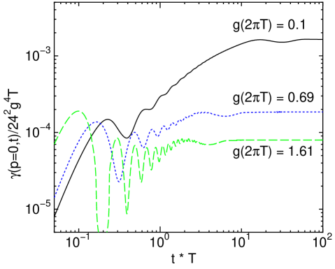
FIG. 3.: The time dependence of $\gamma(\mbox{\boldmath$p$}=0,t)/(24g^{2})^{2}T$ for three values of the coupling constant, $g(2\pi T)=0.1\,({\mathrm{s}olid})$, $0.69\,({\mathrm{d}otted})$ and $1.61\,({\mathrm{d}ashed})$.

In Fig. 3, $\gamma(\mbox{\boldmath$p$}=0,t)/24^{2}g^{4}T$ is plotted as a function of $t\cdot T$ for three values of the coupling constant $g(2\pi T)=0.1,0.69$ and $1.61$. As we can see, for all values of the coupling constant, $\gamma(\mbox{\boldmath$p$}=0,t)$ oscillates in early time and then approaches to some constant value which corresponds to the value in the infinite-time limit, i.e. $\gamma_{\infty}(\mbox{\boldmath$p$}=0)$. As the coupling constant is larger, it is quicker for $\gamma(\mbox{\boldmath$p$}=0,t)$ to end oscillating.

C Decay of single particle excitation: comparison between the cases with and without memory effect

Now let us examine the time evolution of the distribution function with/without the memory effect. Below, we will call $\delta N(\mbox{\boldmath$p$}=0,t)$ obtained from (28) “Markovian result” and that from (30) “non-Markovian result”, and make a comparison between Markovian and non-Markovian results for several values of the coupling constant.

1 Weak coupling regime

Figure 4 shows the time evolutions of $\delta N(\mbox{\boldmath$p$}=0,t)$ for the weak coupling $g(2\pi T)=0.1$. As we can see, the Markovian and non-Markovian results agree completely. This is because a separation of scales is satisfied in the weak coupling regime: the relaxation time is much larger than the time at which the oscillation of the time-dependent damping rate ends. For $g(2\pi T)=0.1$, the relaxation time (times $T$) is about $4300$, and oscillation of $\gamma(\mbox{\boldmath$p$}=0,t)$ ends at $t\cdot T\sim 20$, as read directly from Figs. 4 and 3. In this case, $\delta N(\mbox{\boldmath$p$}=0,t)$ essentially obeys the on-shell Boltzmann equation (38) and represents the exponential damping (39) in both cases.

FIG. 4.: $\delta N(\mbox{\boldmath$p$}=0,t)/\delta N(\mbox{\boldmath$p$}=0,0)$ for Markovian and Non-Markovian results is plotted as a function of $t\cdot T$. Non-Markovian result has been divided by $10$.

2 Moderately large coupling regime

In Fig. 5, $\delta N(\mbox{\boldmath$p$}=0,t)/\delta N(\mbox{\boldmath$p$}=0,0)$ is plotted as a function of $t\cdot T$ in the moderately large coupling regime, $g(2\pi T)=0.69,0.91$ and $1.02$. In this regime, relaxation for the non-Markovian case is faster than that for the Markovian case, which is consistent with the results from the KB equations in 2+1 dimensions [19].

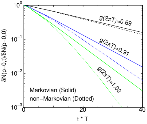
FIG. 5.: Similar to Fig. 4 for the coupling constant $g(2\pi T)=0.69,0.91$ and $1.02$ from the top to the bottom. Solid and dotted lines represent Markovian and non-Markovian results.

3 Strong coupling regime: Oscillation of the distribution function

For the strong coupling constants $g(2\pi T)=1.04,1.20$ and $1.61$, Fig. 6 shows absolute values of $\delta N(\mbox{\boldmath$p$}=0,t)/\delta N(\mbox{\boldmath$p$}=0,0)$ as a function of $t\cdot T$. We observe that $\delta N(\mbox{\boldmath$p$}=0,t)$ for the non-Markovian case oscillates around zero for $g\geq 1.04$. As we can see in the middle panel, relaxation for Markovian and non-Markovian cases equals at $g\sim 1.2$. Then, relaxation for the non-Markovian case becomes slower than that for the Markovian case, as read from the bottom panel.

FIG. 6.: Absolute values of $\delta N(\mbox{\boldmath$p$}=0,t)/\delta N(\mbox{\boldmath$p$}=0,0)$ for Markovian (solid lines) and non-Markovian (dotted lines) are plotted as a function of $t\cdot T$ for the coupling constant $g(2\pi T)=1.04,1.20$ and 1.61, from the top to the bottom panels.

D Discussion

Only in the weak coupling regime where damping of the excitation is exponential, the relaxation time $\tau_{\mathrm{rel}}$ can be obtained by an exponential fitting

$$\delta N(\mbox{\boldmath$p$},t)\sim\exp\left(-\tau_{\mathrm{rel}}^{-1}\cdot t\right)\,.$$ (56)

In the moderately large and the strong coupling regimes, especially in the region where $\delta N$ oscillates, we can not define the relaxation time of the zero mode in a precise sense. The important point, however, is that an opposing influence of the memory effect on relaxation of the excitation is observed as the coupling constant changes, as you can see in Figs. 5 and 6.

Referring to the discussion in the weak coupling regime, it should be noted that the memory effect can affect the relaxation time even in the region where the separation of scales is satisfied well. For $g=0.69$, although the relaxation time ($\sim 23\cdot T$) in Fig. 5 is larger than $\sim 3\cdot T$ at which the oscillation of $\gamma(\mbox{\boldmath$p$},t)$ ends in Fig. 3, there is the onset of the memory effect, that is, there is a slight difference between Markovian and non-Markovian results. Therefore, it is expected that the separation of scales works only in the adequately weak coupling.

In Fig. 6, as the coupling constant increases, the relaxation time for the non-Markovian results seems inclined to saturate. On the other hand, the Markovian results show a monotone decreasing of the relaxation time. In order to see whether the relaxation time saturates, we need to study the time evolution for stronger coupling $g>1.6$, which is computable in the same way. However, such a strong coupling brings about the possibility of conflicting with the quasiparticle approximation used in our calculations, as mentioned below. Therefore, we don’t make further consideration for the possibility of a saturation of the relaxation time here, which is an important future work.

Throughout the present paper, we have used the quasiparticle approximation in which an excitation has an infinite lifetime. The validity of this approximation requires the condition that the relaxation time is larger than $1/\omega_{\mbox{\boldmath$p$}}$ ($=1/M$ for zero mode), which corresponds to a long-lived excitation [30]. In the range of the coupling constant in our calculations, this condition are satisfied. In order to examine the case of stronger coupling constant, it is needed to include the dynamical spectral function with the finite width, which is outside the present scope.

IV Summary and outlook

Based on the kinetic equations with/without the memory effect, we studied the role of that effect in decay of the single particle excitation of $\phi^{4}$ theory. Starting from the two-particle irreducible effective action of the three-loop approximation and corresponding Kadanoff-Baym equations, we derived the kinetic equations into which the memory effect was incorporated by the GKB ansatz proposed by P. Lipavsky, V. Spicka, and B. Velicky [27]. It was observed in numerical results that, while relaxation of the excitation is unaffected by the memory effect in the weak coupling regime, this effect influences it differently as the coupling constant increases: The memory effect leads to faster relaxation for the moderately large coupling and to slower relaxation for $g>1.2$. It is expected that the effect of memory manifests itself in totally nonequilibrium situation, that is, in non-linear kinetic equations for the distribution functions. The important point is that, although we adopted a simple $\phi^{4}$ model, the influence of the memory effect on relaxation is probably universal in strongly correlated plasmas. In particular, our results suggest a possibility of the saturation of the relaxation time.

Finally, some comments are in order. The spectral function used in this paper is the quasiparticle one and cannot be applicable to the system where the relaxation time is shorter than $1/\omega_{\mbox{\boldmath$p$}}$. In order to study the effect of the finite width in the spectral function, it would be necessary to use the phenomenological treatment such as an extended quasiparticle picture [32, 39], or to solve directly KB equations for two-point Green’s functions [13, 14, 15, 16, 18, 19]. Two-time Green’s functions in KB equations involve the information about the dynamical spectral function having the finite width as well as the one-particle distribution function. Furthermore, study of the linear sigma model or the fermionic system with the chiral phase transition is also an important future project in our approach, which might be related to Heavy-ion collision experiments.

REFERENCES

- [1] See, for example, H. Satz, Nucl. Phys. A 681, 3 (2001); Nucl. Phys. A 661, 104 (1999).
- [2] D. T. Son, Phys. Rev. D 54, 3745 (1996).
- [3] S. Y. Khlebnikov and I. I. Tkachev, Phys. Rev. Lett. 79, 1607 (1997); Phys. Rev. Lett. 77, 219 (1996).
- [4] R. Micha and I. I. Tkachev, Phys. Rev. Lett. 90, 121301 (2003).
- [5] G. N. Felder and I. Tkachev, arXiv:hep-ph/0011159.
- [6] G. N. Felder and L. Kofman, Phys. Rev. D 63, 103503 (2001).
- [7] L. D. McLerran and R. Venugopalan, Phys. Rev. D 49, 2233 (1994); Phys. Rev. D 49, 3352 (1994).
- [8] A. H. Mueller, Phys. Lett. B 475, 220 (2000); Nucl. Phys. B 572, 227 (2000).
- [9] R. Baier, A. H. Mueller, D. Schiff and D. T. Son, Phys. Lett. B 502, 51 (2001); R. Baier, A. H. Mueller, D. T. Son and D. Schiff, Nucl. Phys. A 698, 217 (2002); R. Baier, A. H. Mueller, D. Schiff and D. T. Son, Phys. Lett. B 539, 46 (2002).
- [10] G. R. Shin and B. Muller, J. Phys. G 29, 2485 (2003); J. Phys. G 28, 2643 (2002).
- [11] P. Arnold, J. Lenaghan and G. D. Moore, JHEP 0308, 002 (2003).
- [12] L. P. Kadanoff and G. Baym, Quantum Statistical Mechanics (Benjamin, New York, 1962).
- [13] G. Aarts and J. Berges, Phys. Rev. D 64, 105010 (2001).
- [14] J. Berges and J. Cox, Phys. Lett. B 517, 369 (2001).
- [15] J. Berges, Nucl. Phys. A 699, 847 (2002).
- [16] J. Berges and J. Serreau, Phys. Rev. Lett. 91, 111601 (2003); arXiv:hep-ph/0302210.
- [17] F. Cooper, J. F. Dawson and B. Mihaila, Phys. Rev. D 67, 056003 (2003).
- [18] J. Berges, S. Borsanyi and J. Serreau, Nucl. Phys. B 660, 51 (2003).
- [19] W. Cassing and S. Juchem, arXiv:hep-ph/0308066; S. Juchem, W. Cassing and C. Greiner, arXiv:hep-ph/0307353.
- [20] D. Boyanovsky, I. D. Lawrie and D. S. Lee, Phys. Rev. D 54, 4013 (1996).
- [21] D. Boyanovsky, C. Destri, H. J. de Vega, R. Holman and J. Salgado, Phys. Rev. D 57, 7388 (1998).
- [22] D. Boyanovsky, H. J. de Vega and S. Y. Wang, Phys. Rev. D 61, 065006 (2000).
- [23] D. Boyanovsky, C. Destri and H. J. de Vega, arXiv:hep-ph/0306124.
- [24] G. Aarts, G. F. Bonini and C. Wetterich, Nucl. Phys. B 587, 403 (2000).
- [25] M. Salle, J. Smit and J. C. Vink, Nucl. Phys. B 625, 495 (2002); Phys. Rev. D 64, 025016 (2001).
- [26] N. Ikezi, M. Asakawa and Y. Tsue, arXiv:nucl-th/0310035.
- [27] P. Lipavsky, V. Spicka, and B. Velicky, Phys. Rev. B 34, 6933 (1986)
- [28] J. S. Schwinger, J. Math. Phys. 2, 407 (1961).
- [29] L. V. Keldysh, Zh. Eksp. Teor. Fiz. 47, 1515 (1964) [Sov. Phys. JETP 20, 1018 (1965)].
- [30] J. P. Blaizot and E. Iancu, Phys. Rept. 359, 355 (2002).
- [31] H. S. Kohler and K. Morawetz, Phys. Rev. C 64, 024613 (2001); K. Morawetz and H. S. Kohler, Eur. Phys. J. A 4, 291 (1999).
- [32] H. S. Kohler Phys. Rev. E 53, 3145 (1996); Phys. Rev. C 51, 3232 (1995); Nucl. Phys. A 583, 339 (1995).
- [33] R. R. Parwani, Phys. Rev. D 45, 4695 (1992) [Erratum-ibid. D 48, 5965 (1993)].
- [34] S. Jeon, Phys. Rev. D 52, 3591 (1995).
- [35] E. k. Wang and U. W. Heinz, Phys. Rev. D 53, 899 (1996).
- [36] J. P. Blaizot, E. Iancu and A. Rebhan, Phys. Rev. D 63, 065003 (2001).
- [37] I. T. Drummond, R. R. Horgan, P. V. Landshoff and A. Rebhan, Nucl. Phys. B 524, 579 (1998).
- [38] H. van Hees and J. Knoll, Phys. Rev. D 65, 025010 (2002); Phys. Rev. D 65, 105005 (2002); Phys. Rev. D 66, 025028 (2002).
- [39] V. Spicka and P. Lipavsky, Phys. Rev. Lett. 73, 3439 (1994); Phys. Rev. B 52, 14615 (1995),