$\pi\pi$ Scattering in Three Flavour ChPT

Abstract:

We present the scattering lengths for the $\pi\pi$ processes in the three flavour Chiral Perturbation Theory (ChPT) framework at next-to-next-to-leading order. We then combine this calculation with the determination of the parameters from $K_{e4}$ and the masses and decay constants and compare with the results of a dispersive analysis of $\pi\pi$ scattering. The comparison indicates a small but nonzero value for the $1/N_{c}$ suppressed NLO low energy constants $L_{4}^{r}$ and $L_{6}^{r}$.

1 Introduction

The $\pi\pi$ scattering amplitude is one of the fundamental observables in low energy particle physics and has been since long the subject of many studies. The pions are the lightest strongly interacting particles and have thus a special status. Their properties are also strongly influenced by the chiral symmetry present in the limit of massless quarks in Quantum Chromo Dynamics (QCD).

In this paper we add one more step in the discussion of pion properties. We calculate $\pi\pi$ scattering in three flavour Chiral Perturbation Theory (ChPT) in order to complete the connection between the $K_{\ell 4}$ form factors and $\pi\pi$ scattering following from chiral symmetry. We stay in the isospin limit here and neglect electromagnetic effects. But first we give a short historical overview of chiral symmetry relevant to $\pi\pi$ scattering.

Chiral symmetry was introduced a long time ago and used in the form of current algebra and the PCAC assumptions (partial conservation of axial currents.) Weinberg [1] used these methods to derive a result for $\pi\pi$ scattering valid to lowest order in meson masses and momenta. It was later realized that the assumptions of analyticity used in many PCAC type of analyses were not always true. This allowed to calculate often the leading nonanalytic corrections to the lowest order PCAC results. This line of work within the PCAC methods has been reviewed in Ref. [2] where also references to earlier work can be found. The more modern method of using chiral symmetry in the form of an effective field theory was introduced by Weinberg [3] and systematized by Gasser and Leutwyler [4]. This is now known as ChPT. They performed the full next-to-leading order (NLO) calculation of $\pi\pi$ scattering [5] as the first major application. The parameters necessary for determining the $\pi\pi$ scattering lengths at threshold had to be taken from the $D$ wave experimental results. A reasonable agreement with the experimental result was obtained. Gasser and Leutwyler also extended ChPT to the three flavour sector including the strange quark in addition to the up and down quark in the ChPT formalism [6]. This allowed to determine the parameters necessary for prediction $\pi\pi$ scattering to be determined from the absolute values of the form factors in $K_{\ell 4}$ decays. Note that the phase and the absolute values are in principle separately measurable quantities there such that the relation between the phase as determined by the relevant $\pi\pi$ scattering phase and the absolute value is not a trivial prediction. These NLO calculations of $K_{\ell 4}$ decays were performed and again led to a reasonable agreement with the known values [7, 8]. The three flavour expression for $\pi\pi$ scattering was first calculated in [9] and later independently in [10].

The first step at next-to-next-to-leading order (NNLO) was done in Ref. [10] where the dispersive part of the amplitude was determined. The full two loop calculation in two flavour ChPT was performed in Ref. [11, 12]. The NNLO calculation of $K_{\ell 4}$ has also been performed [13, 14] and was used to study $\pi\pi$ scattering via the two flavour NNLO calculation using the relation between the NLO order parameters in two and three flavour ChPT derived in Ref. [4]. This still leaves an uncertainty since in order to have full control at NNLO the corrections to those relations need also to be determined. This can be done in principle by integrating out the kaons and eta degrees of freedom out of the three flavour ChPT NNLO generating functional but this has not been done so far. Alternatively one can directly calculate the NNLO amplitude for $\pi\pi$ scattering in three flavour ChPT. This is what has been done in this paper.

A different way to describe theoretically $\pi\pi$ scattering is to use the constraints from analyticity and unitarity. These lead to many different sum rules but especially after crossing properties have been included the resulting set of equations becomes very constraining. These are known as the Roy equations [15]. They were analyzed extensively in the seventies, see e.g. [16]. The available high energy data together with the Roy equations allowed to describe $\pi\pi$ scattering in terms of two parameters usually chosen to be the scattering lengths in the $S$ wave channel for isospin 0 and 2, $a_{0}^{0}$ and $a^{2}_{0}$ respectively. $a_{0}^{0}$ was then essentially fixed by measuring the difference in phase of the $K_{e4}$ form factors. This measurement has been dominated for a long time by the experiment of Ref. [17]. The result was in disagreement with the Weinberg prediction [1] but in borderline agreement with the NLO order one [5]. However, the central values was rather different from the ChPT prediction. If this central value turned out to be correct, the consequences for the low energy structure of QCD would be quite strong. In particular the chiral symmetry breaking might not be driven by the simple quark anti-quark condensate, see [18] and references therein. This was the origin for the renewed interest in $\pi\pi$ scattering. The analysis of the Roy equations has been updated in Ref. [19]. This was then combined with the constraints from chiral symmetry in Ref. [20, 21]. The constraints used were the solutions of the Roy equations of [19], the ChPT two flavour calculations of $\pi\pi$ scattering [11, 12] and the pion scalar form factor [22]. It also used the method of determination of low energy constants from sum rules over $\pi\pi$ phases from [23]. This analysis led to very constrained predictions for the scattering lengths. These were confirmed nicely by the E865 experiment at BNL [26, 27]. A similar analysis but without the constraint from the pion scalar radius can be found in [28].

In this paper we will compare the predictions for the $\pi\pi$ scattering lengths in three flavour ChPT with the experimental input from $K_{\ell 4}$ decays to NNLO. We find an acceptable agreement as discussed in Sect. 6.

In two flavour ChPT it is clear now that spontaneous chiral symmetry breaking goes through the quark anti-quark condensate [20, 21]. There is still a possibility that the behaviour when also the strange quark mass goes through zero, is qualitatively different. This is discussed in the recent work by Stern and collaborators [29, 30]. The argument is that large disconnected loop contributions from strange quarks, via kaons and etas, can be large, making a convergent three flavour ChPT difficult to achieve in the usual sense [30, 31]. This has been studied in some detail in [14] and also in the context of the three flavour ChPT calculations of the various scalar form factors [32]. The masses and decay constants, see Ref. [33] and references therein, showed the possibility of this behaviour. The various vector form factors calculated did not seem to have problems with convergence [34, 35, 36, 37]. It turns out that this calculation does not provide much more information than the scalar form factors [32] did. Work is in progress to extend the $\pi K$ scattering also to NNLO. This might allow us to shed more light on this issue.

This paper is organized as follows. In Sect. 2 we give a short overview of ChPT and the references for the methods of NNLO calculations. In Sect. 3 the general properties of the $\pi\pi$ scattering amplitude are described and the quantities used later defined. Sect. 4 gives an overview of our main result, the calculation of the $\pi\pi$ scattering amplitude to NNLO in three flavour ChPT. We also present here some plots showing the importance of the various contributions. The inputs we use to do the numerical analysis are described in Sect. 5. The main numerical analysis is presented in Sect. 6 and we give our main conclusions in Sect. 7. The appendices are devoted to giving references about the various loop integrals used in this work and the explicit expressions at NNLO for $\pi\pi$ scattering.

2 Chiral Perturbation Theory

ChPT is the effective field theory for QCD at low energies introduced by Weinberg, Gasser and Leutwyler [3, 4, 6]. Introductory lectures can be found in Ref. [38]. This leads to an expansion in quark masses and meson momenta generically labeled $p$ and assumes $m_{q}\sim p^{2}$ since for an on-shell meson $p_{\pi}^{2}=m_{\pi}^{2}$. The ChPT formalism exists both for two light flavours, up and down, referred to as $SU(2)$ ChPT, and for three light flavours, up, down and strange, referred to as $SU(3)$ ChPT. The Lagrangian for the strong and semi leptonic mesonic sector to NNLO can be written as

$${\cal L}={\cal L}_{2}+{\cal L}_{4}+{\cal L}_{6}\,,$$ (1)

where the subscript refers to the chiral order. The lowest order Lagrangian is

$${\cal L}_{2}=\frac{F_{0}^{2}}{4}\langle u_{\mu}u^{\mu}+\chi_{+}\rangle\,.$$ (2)

The mesonic fields enter via

$$u=\exp\left(\frac{iM}{F_{0}\sqrt{2}}\right)\,,\quad M=\left(\begin{array}[]{ccc}\frac{1}{\sqrt{2}}\pi^{0}+\frac{1}{\sqrt{6}}\eta&\pi^{+}&K^{+}\\ \pi^{-}&\frac{-1}{\sqrt{2}}\pi^{0}+\frac{1}{\sqrt{6}}\eta&K^{0}\\ K^{-}&\overline{K^{0}}&\frac{-2}{\sqrt{6}}\eta\end{array}\right)\,$$ (3)

and the quantity $u_{\mu}$ also contains the external vector ($v_{\mu}$) and axial-vector ($a_{\mu}$) currents

$$u_{\mu}=i(u^{\dagger}\partial_{\mu}u-\partial_{\mu}uu^{\dagger}-iu^{\dagger}r_{\mu}u+iul_{\mu}u^{\dagger})\,,\quad l_{\mu}(r_{\mu})=v_{\mu}-(+)a_{\mu}\,.$$ (4)

The scalar ($s$) and pseudo scalar ($p$) currents are contained in

$$\chi_{\pm}=u^{\dagger}\chi u^{\dagger}\pm u\chi^{\dagger}u\,,\quad\chi=2B_{0}\left(s+ip\right)\,.$$ (5)

The $p^{4}$ or NLO Lagrangian, ${\cal L}_{4}$, was introduced in Ref. [6] and reads

$${\cal L}_{4} = \hskip 9.67383ptL_{1}\langle u_{\mu}u^{\mu}\rangle^{2}+L_{2}\langle u_{\mu}u_{\nu}\rangle\langle u^{\mu}u^{\nu}\rangle$$ (6)

$$+L_{3}\langle u^{\mu}u_{\mu}u^{\nu}u_{\nu}\rangle+L_{4}\langle u^{\mu}u_{\mu}\rangle\langle\chi_{+}\rangle$$

$$+L_{5}\langle u^{\mu}u_{\mu}\chi_{+}\rangle+L_{6}\langle\chi_{+}\rangle^{2}$$

$$+L_{7}\langle\chi_{-}\rangle^{2}+L_{8}\langle\chi_{+}\chi_{-}\rangle$$

$$-iL_{9}\langle F^{R}_{\mu\nu}uu^{\mu}u^{\nu}u^{\dagger}+F^{L}_{\mu\nu}u^{\dagger}u^{\mu}u^{\nu}u\rangle+L_{10}\langle F^{R}_{\mu\nu}UF^{L\mu\nu}U^{\dagger}\rangle$$

$$+H_{1}\langle F_{\mu\nu}^{R}F^{\mu\nu R}+F_{\mu\nu}^{L}F^{\mu\nu L}\rangle+H_{2}\langle\chi_{+}^{2}-\chi_{-}^{2}\rangle/4\,.$$

The $L_{9}$ and $L_{10}$ terms introduce also the field strength tensor

$$F_{\mu\nu}^{L(R)}=\partial_{\mu}l(r)_{\nu}-\partial_{\nu}l(r)_{\mu}-i\left[l(r)_{\mu},l(r)_{\nu}\right]\,.$$ (7)

The two terms proportional to $H_{1}$ and $H_{2}$ are high energy contact terms and are not involved in physical amplitudes, $L_{9}$ and $L_{10}$ play only a minor role for the quantities discussed in this paper.

We quote the schematic form of the NNLO Lagrangian in the three flavour case

$${\cal L}_{6}=\sum_{i=1,94}C_{i}\,O_{i}$$ (8)

and refer to [39] for their explicit expressions. The last four terms are contact terms [39].

The ultra-violet divergences produced by loop diagrams of order $p^{4}$ and $p^{6}$ cancel in the process of renormalization with the divergences extracted from the low energy constants $L_{i}$’s and $C_{i}$’s. We use dimensional regularization and the modified minimal subtraction $(\overline{MS})$ version usually used in ChPT. An extensive description of the regularization and renormalization procedure including the freedom involved can be found in Refs. [12] and [40].

The subtraction of divergences is done explicitly by

$$L_{i}=(c\mu)^{d-4}[\hat{\Gamma}_{i}\Lambda+L_{i}^{r}(\mu)]$$ (9)

and

$$C_{i}=\frac{(c\mu)^{2(d-4)}}{F^{2}}\left[C_{i}^{r}(\mu)-\left(\Gamma_{i}^{(1)}+\Gamma_{i}^{(L)}(\mu)\right)\Lambda-\Gamma_{i}^{(2)}\Lambda^{2}\right]$$ (10)

where $c$ and $\Lambda$ are defined by

$$\ln{c}=-\frac{1}{2}\left[\ln{4\pi}+\Gamma^{\prime}(1)+1\right]\,,$$ (11)

$$\Lambda=\frac{1}{16\pi^{2}(d-4)}\,.$$ (12)

The coefficients $\hat{\Gamma}_{i}$, $\Gamma_{i}^{(1)}$ and $\Gamma_{i}^{(2)}$ are constants while the $\Gamma_{i}^{(L)}$ ’s are linear combinations of the $L_{i}^{r}(\mu)$ ’s. Their explicit expressions can all be found in [40] where they have been calculated in general. The NLO divergences were first calculated in Ref. [4, 6] and the doubles poles at NNLO first in Ref. [41].

3 The $\pi\pi$ amplitude: general properties

The $\pi\pi$ scattering amplitude in all the relevant channels can be written as a function $A(s,t,u)$ which is symmetric in the last two arguments:

$$A\left(\pi^{a}(p_{1})\pi^{b}(p_{2})\to\pi^{c}(p_{3})\pi^{d}(p_{4})\right)=\delta^{ab}\delta^{cd}A(s,t,u)+\delta^{ac}\delta^{bd}A(t,u,s)+\delta^{ad}\delta^{bc}A(u,t,s)\,.$$ (13)

$s,t,u$ are the usual Mandelstam variables

$$s=(p_{1}+p_{2})^{2}\,\quad t=(p_{1}-p_{3})^{2}\quad\mbox{and}\quad u=(p_{1}-p_{4})^{2}\,.$$ (14)

The various isospin amplitudes $T^{I}$ can be written in terms of this function as

$$T^{0}(s,t) = 3A(s,t,u)+A(t,u,s)+A(u,s,t)\,,$$

$$T^{1}(s,t) = A(t,u,s)-A(u,s,t)\,,$$

$$T^{2}(s,t) = A(t,u,s)+A(u,s,t)\,,$$ (15)

where the kinematical variables $t,u$ can be expressed in terms of $s$ and $\cos\theta$ as

$$t=-\frac{1}{2}(s-4m_{\pi}^{2})(1-\cos\theta)\,,\quad u=-\frac{1}{2}(s-4m_{\pi}^{2})(1+\cos\theta)\,.$$ (16)

The various amplitudes can be expanded in partial waves via

$$T^{I}(s,t)=32\pi\sum_{\ell=0}^{\infty}(2\ell+1)P_{\ell}(\cos\theta)t^{I}_{\ell}(s)\,.$$ (17)

Near threshold these are expanded in terms of the threshold parameters

$$t^{I}_{\ell}=q^{2\ell}\left(a^{I}_{\ell}+b^{I}_{\ell}q^{2}+{\cal O}(q^{4})\right)\,,\quad q^{2}=\frac{1}{4}\left(s-4m_{\pi}^{2}\right)\,.$$ (18)

Below the inelastic threshold the partial waves satisfy

$$\mbox{Im}t^{I}_{\ell}(s)=\sigma(s)\left|t^{I}_{\ell}(s)\right|^{2},\quad\quad\sigma(s)=\sqrt{1-\frac{4m_{\pi}^{2}}{s}}\,.$$ (19)

In this regime the partial waves can be written in terms of the phase-shifts as

$$t^{I}_{\ell}(s)=\frac{1}{\sqrt{1-(4m_{\pi}^{2}/s)}}\,\frac{1}{2i}\left\{e^{2i\delta^{I}_{\ell}(s)}-1\right\}\,.$$ (20)

In ChPT the inelasticity only starts at order $p^{8}$. The $p^{2}$ result has only nonzero items for $t^{0}_{0}$, $t^{1}_{1}$ and $t^{2}_{0}$. As a consequence the imaginary parts for all other partial waves starts only at order $p^{8}$. In [18] it has been shown that thus up to order $p^{8}$ the amplitude can be written as

$$A(s,t,u) = C(s,t,u)+32\pi\Bigg{(}\frac{1}{3}V^{0}(s)+\frac{3}{2}(s-u)V^{1}(t)+\frac{3}{2}(s-t)V^{1}(u)$$ (21)

$$+\frac{1}{2}V^{2}(t)+\frac{1}{2}V^{2}(u)-\frac{1}{3}V^{2}(s)\Bigg{)}\,.$$

The function $V^{I}(s)$ have a polynomial ambiguity but we have chosen to keep it in this more general form. The $V^{I}(s)$ contain the singularities in the $\pi\pi$ amplitudes from intermediate states with isospin $I$ in the various channels. They obey the relations

$$\mbox{Im}V^{0,2}(s)=\mbox{Im}t^{0,2}_{0}(s)\,,\quad\quad\mbox{Im}V^{1}(s)=\frac{1}{s-4m_{\pi}^{2}}\mbox{Im}t^{1}_{1}(s)\,.$$ (22)

The polynomial $C(s,t,u)$ can be written using $s+t+u=4m_{\pi}^{2}$ in the form

$$C(s,t,u)=c_{1}+c_{2}s+c_{3}s^{2}+c_{4}(t-u)^{2}+c_{5}s^{3}+c_{6}s(t-u)^{2}\,.$$ (23)

4 ChPT results

4.1 Two Flavour ChPT

The lowest order was derived by Weinberg [1] a long time ago and corresponds to

$$c_{1}=\frac{m_{\pi}^{2}}{F_{\pi}^{2}}\,,\quad\quad c_{2}=-\frac{1}{F_{\pi}^{2}}\,,$$ (24)

in (23). The next order was derived by Gasser and Leutwyler [5] and the full calculation of order $p^{6}$ was performed in [11, 12].

4.2 Three Flavour ChPT

The lowest order is identical to the two-flavour case of Eq. (24). The order $p^{4}$ $\pi\pi$ scattering amplitude in three flavour ChPT was first published in [9] App. A. It can also be found in [10]. Notice that the contribution from $L_{1}^{r}$ and $L_{3}^{r}$ is missing in [9]. Our result at this order is in full agreement with the corrected version. We have expressed the result in terms of the functions defined in Eq. ( 21) in App. B.

The $p^{6}$ expressions we present are those corresponding to the $p^{4}$ results expressed in the physical masses and decay constants. The order $p^{6}$ expression is our main result. Expressed in the polynomial $C(s,t,u)$ and the functions $V^{0,1,2}(s)$ it is shown in App. B.

4.3 A first numerical look

In this subsection we present a first look at the numerical results for the two loop amplitudes. We choose as input the pion decay constant, the charged pion mass, an averaged kaon mass with electromagnetic effects removed and the physical eta mass.

$$F_{\pi} = 92.4~{}\mbox{MeV}\,,\quad m_{\pi}=m_{\pi^{+}}=139.56995~{}\mbox{MeV}\,,$$

$$m_{K} = 494.53~{}\mbox{MeV}\,,\quad m_{\eta}=547.3~{}\mbox{MeV}\,.$$ (25)

The subtraction scale $\mu=770~{}\mbox{MeV}$ is used throughout the paper unless otherwise mentioned explicitly.

We first compare the $SU(2)$ and $SU(3)$ ChPT results for the three main partial waves for all low energy constants set to zero at the scale 770 MeV. So we set $L_{i}^{r}=C_{i}^{r}=l_{i}^{r}=c_{i}^{r}=0$ and compare the pure loop results for the $SU(2)$ and $SU(3)$ ChPT.

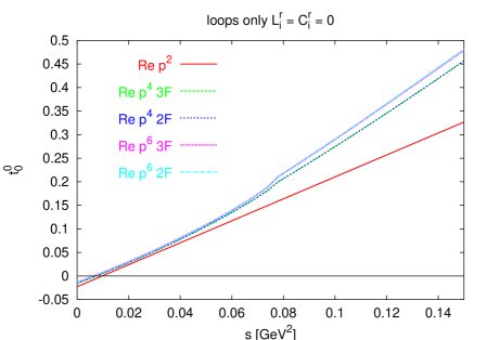
Figure 1: Results for the $t^{0}_{0}$ partial wave: The $SU(2)$ ChPT results of [12] for all LECs equal to zero, labeled 2F, compared to the results for the $SU(3)$ ChPT results also for all LECs equal to zero at $\mu=770~{}\mbox{MeV}$, labeled 3F.

In Fig. 1 we have plotted the partial wave amplitude $t^{0}_{0}(s)$ Notice the extremely small difference between the two results, showing that this channel is obviously dominated by the pion loops and the kaon and eta have only a fairly small effect.

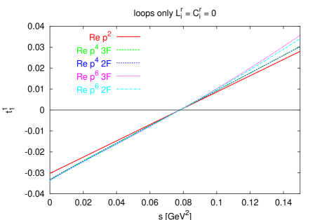
Figure 2: Results for the $t^{1}_{1}$ partial wave: The $SU(2)$ ChPT results of [12] for all LECs equal to zero, labeled 2F, compared to the results for the $SU(3)$ ChPT results also for all LECs equal to zero at $\mu=770~{}\mbox{MeV}$, labeled 3F.

For the $t^{1}_{1}$ partial wave, shown in Fig. 2 the order $p^{4}$ results are very similar in both cases again but there is somewhat more difference in the order $p^{6}$ contributions, this channel has a much stronger effect from the LECs, see below, so this difference does not play much of a role.

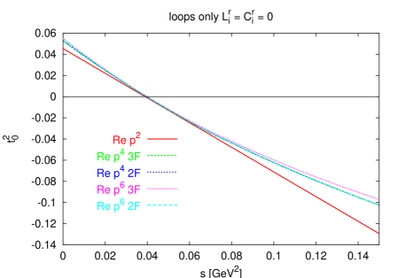
Figure 3: Results for the $t^{2}_{0}$ partial wave: The $SU(2)$ ChPT results of [12] for all LECs equal to zero, labeled 2F, compared to the results for the $SU(3)$ ChPT results also for all LECs equal to zero at $\mu=770~{}\mbox{MeV}$, labeled 3F.

The $t^{2}_{0}$ amplitude, shown in Fig. 3 has a somewhat more surprising difference. Again the order $p^{4}$ results for the $SU(2)$ and $SU(3)$ cases are very similar but the $p^{6}$ pure loop correction is rather different. We will come back to this later.

That the difference at order $p^{4}$ would be small was of course expected. In [12] the contribution from the $p^{4}$ loops from kaons and etas was estimated and found to be very small.

5 Solution of the Roy Equations and Other Inputs

For the experimental values of the $\pi\pi$ scattering phase-shifts we use the results from the extensive analysis of the Roy equations done in [19]. This analysis has been checked with somewhat relaxed input assumptions in [28]. These equations and the input are constrained in such a way that the $\pi\pi$ phase-shifts are determined as a function of two input parameters chosen to be the scattering lengths $a^{0}_{0}$ and $a^{2}_{0}$.

The solution of the Roy equations has been used in [20, 21] together with the constraints from the $SU(2)$ ChPT $p^{6}$ expression to obtain a precise prediction of $a^{0}_{0}$ and $a^{2}_{0}$. The input used there was the pion scalar radius evaluated using dispersive methods and the estimates of the $p^{6}$ low energy constants of [12], together with the $SU(2)$ order $p^{6}$ calculations of $\pi\pi$ scattering [11, 12] and the pion scalar radius [22].

The conclusions of that analysis have been challenged in [24], the reply of the authors of [20, 21] can be found in [25].

For our $SU(3)$ ChPT results we use as inputs the masses and decay constants given in Sect. 4.3 and a subtraction constant $\mu=770$ MeV. We work in the limit of exact isospin.

It should be mentioned that these numbers were obtained using a general refit of all the other $L_{i}^{r}$ with a fixed $L_{4}^{r}$ and $L_{6}^{r}$ as input. The inputs were the absolute values of the $K_{\ell 4}$ form factors as measured by the E865 experiment [26, 27], decay constants and meson masses. The fits correspond precisely to those of fit 10 in [42] but with different input values for $L_{4}^{r}$ and $L_{6}^{r}$.

For the constants at order $p^{6}$ we need to use input values using various estimates. The method used was proposed at NLO in Ref. [43, 44] and references therein. We do not estimate here the NLO constants this way but only NNLO. The places where comparisons with experiment are available are in general reasonable agreement with these estimates. The estimates are obtained by including the main resonance exchange contributions and putting the $p^{6}$ part of these amplitudes equal to the contribution from the $C_{i}^{r}$. This procedure is obviously subtraction point dependent and is normally only performed to leading order in the expansion in $1/N_{c}$, with $N_{c}$ the number of colours. Alternative approaches exist but we will not discuss them here. Recent papers addressing this type of issues are [45, 46, 47] and references therein. A systematic study of this issue is clearly important, for our present purpose the estimates seem sufficient.

The estimates from resonance exchange for the masses and decay constants are the most uncertain. These are discussed in [33] and [45]. For the numerical results used here they have been put to zero, the naive size estimate of [33] led to extremely large NNLO corrections. The estimates of the $K_{\ell 4}$ amplitudes can be found in [14] after the work of [48]. The effect of varying these was studied in [14] and found to be reasonable.

The estimates of the $p^{6}$ contributions to $\pi\pi$ scattering we use are those of [12]. These lead to the contributions to the various threshold parameters given in Table 1. The uncertainty on these is quite considerable but probably within a factor of two, this is also discussed in Ref. [21]. Similar resonance estimates of $\pi\pi$ scattering can be found in [49].

In order to be able to perform a study of the dependence on $L_{4}^{r}$ and $L_{6}^{r}$ we have redone the fits to the masses, decay constants and the $K_{\ell 4}$ absolute values of the form factors with a range of values for $L_{4}^{r}$ and $L_{6}^{r}$. This is similar to the part discussed in [14] but now with the newer experimental input [26, 27] included. The fits correspond exactly to the fit labeled fit 10 in [42] but with various values of $L_{4}^{r}$ and $L_{6}^{r}$ as input. These were already used in Ref. [32] to compare with the scalar form factors. There a general preference was found for the region $L_{6}^{r}\approx L_{4}^{r}-0.0003$. In that region the corrections to the pion scalar form factor at zero were fairly small as well as a good agreement with the pion scalar radius was obtained. It should be kept in mind that all the other $L_{i}^{r}$ are varied together with $L_{4}^{r}$ and $L_{6}^{r}$ in order to fit the mentioned quantities. Reasonable fits were obtained for most values of $L_{4}^{r}$ and $L_{6}^{r}$. Varying $L_{4}^{r}$ and $L_{6}^{r}$ without the correlated changes in the other $L_{i}^{r}$ would lead to much larger variations than the ones shown below.

6 Numerical Analysis

	$p^{2}$	$p^{4},~{}L_{i}^{r}=0$	$p^{6},~{}L_{i}^{r}=C_{i}^{r}=0$	$p^{6},~{}C_{i}^{r}$ only	Ref. [21]
$a^{0}_{0}$	0.159	0.041	0.011	0.001	$0.220\pm 0.005$
$b^{0}_{0}$	0.182	0.075	0.016	0.004	$0.276\pm 0.006$
$10\,a^{2}_{0}$	$-$0.454	0.037	0.015	$-$0.004	$-0.444\pm 0.010$
$10\,b^{2}_{0}$	$-$0.908	0.144	0.029	$-$0.014	$-0.803\pm 0.012$
$10\,a^{1}_{1}$	0.303	0.022	0.025	0.000	$0.379\pm 0.005$
$10\,b^{1}_{1}$	$-$	0.005	0.033	0.000	$0.057\pm 0.001$
$10^{2}\,a^{0}_{2}$	$-$	0.121	0.050	0.001	$0.175\pm 0.003$
$10^{2}\,b^{0}_{2}$	$-$	$-$0.040	$-$0.005	0.005	$-0.036\pm 0.002$
$10^{3}\,a^{2}_{2}$	$-$	0.492	$-$0.187	$-$0.003	$0.170\pm 0.013$
$10^{3}\,b^{2}_{2}$	$-$	$-$0.234	$-$0.136	$-$0.045	$-0.326\pm 0.012$
$10^{4}\,a^{1}_{3}$	$-$	0.20	0.27	0.15	$0.560\pm 0.019$
$10^{4}\,b^{1}_{3}$	$-$	$-$0.15	$-$0.22	$-$	$-0.402\pm 0.018$

Table 1: The various contributions to the threshold parameters defined in (18) with the $L_{i}^{r}=0$ at $\mu=770~{}$MeV. The $C_{i}^{r}$ contribution is shown separately using the estimates of [12]. The threshold parameters are given in the corresponding power of $m_{\pi^{+}}^{2}$. Note that we have given $a^{I}_{\ell}$ and $b^{I}_{\ell}$ always with the same power of ten.

In order to check convergence let us first look at the various contributions with all the low energy constants set to zero at a scale $\mu=770$ MeV. These are shown in Table 1. The angular integrals have been performed using both a 5 point and a 8 point Gaussian integration over $\cos\theta$. In addition the fits were performed numerically over a range of $q^{2}$ above threshold. The numerical errors on the slopes $b^{I}_{\ell}$ for $\ell=2,3$ are of the order of the last digit shown. For all others this error is below the accuracy given. For comparison we have also given the results of Ref. [21] in the last column.

We will now compare with the full analysis of $\pi\pi$ scattering performed with the use of the Roy equations and the $SU(2)$ ChPT results of [20, 21]. In principle we could redo this work with the $SU(3)$ ChPT results as constraints instead. We have chosen not to do so, postponing a possible more detailed comparison till after the inclusion of $\pi K$ scattering results. Since the $SU(3)$ ChPT results contain the pion loops which are the main effects of the $SU(2)$ ChPT calculations and the $SU(3)$ expressions must reduce to the $SU(2)$ expressions in the limit of a large kaon and eta mass and thus satisfy the $SU(2)$ chiral constraints we do not expect such an analysis to differ substantially from the one performed in Ref. [20, 21].

It can already be seen from Table 1 that the lowest order result together with the pure loop contributions only already give quite a good description of the various scattering lengths. The effects of including nonzero values for the low energy constants should explain the difference. Notice that for almost all cases the estimated contributions from the $p^{6}$ constants $C_{i}^{r}$ is rather small. The main effect is thus from the $p^{4}$ constants $L_{i}^{r}$. We will now study the effects of these when they were fitted to other data as described above with fixed values of $L_{4}^{r}$ and $L_{6}^{r}$ as input.

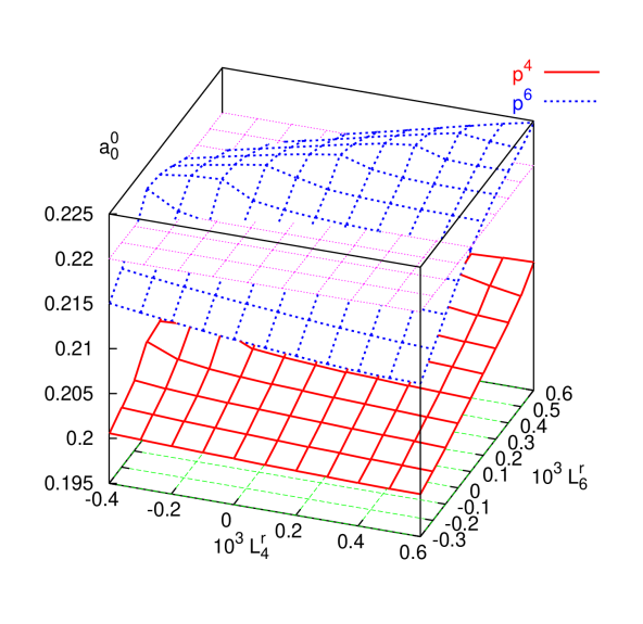
(a)

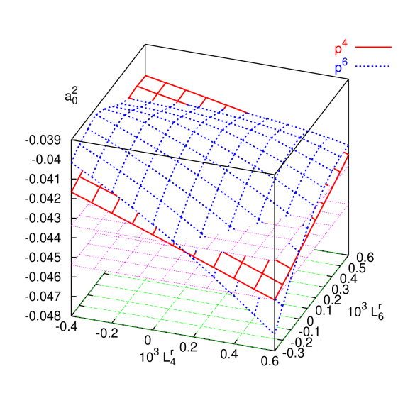
(b)

Figure 4: The scattering lengths $a^{0}_{0}$ and $a^{2}_{0}$ as a function of the input values $L_{4}^{r}$ and $L_{6}^{r}$ with the other $L_{i}^{r}$ simultaneously refitted to the $K_{e4}$ form factors. (a) $a^{0}_{0}$ calculated to order $p^{4}$ and $p^{6}$. The central value of [21] of 0.220 is also shown. (b) $a^{2}_{0}$ at order $p^{4}$ and $p^{6}$. The two horizontal planes indicate the allowed region obtained in [21].

In Fig. 4(a) we have plotted the result for $a^{0}_{0}$ as a function of the input values of $L_{4}^{r}$ and $L_{6}^{r}$. The lowest order value,

$$\left.a^{0}_{0}\right|_{p^{2}}=0.159\,,$$ (26)

is not shown on the plot. The convergence of the series is very good and of similar quality as the two flavour result. Taking the result of [21],

$$\left.a^{0}_{0}\right|_{\cite[cite]{[\@@bibref{}{CGL2}{}{}]}}=0.220\pm 0.005\,,$$ (27)

we see that the agreement is excellent and no new information on $L_{4}^{r}$ and $L_{6}^{r}$ is available from this source, this also confirms the prediction for $a^{0}_{0}$.

The result for $a^{2}_{0}$ is plotted in Fig. 4(b). The lowest order value

$$\left.a^{2}_{0}\right|_{p^{2}}=-0.0454\,,$$ (28)

is not plotted. The series converges well over most of the $L_{4}^{r}$ and $L_{6}^{r}$ range considered. The result should be compared with the result [21],

$$\left.a^{2}_{0}\right|_{\cite[cite]{[\@@bibref{}{CGL2}{}{}]}}=-0.0444\pm 0.0010\,,$$ (29)

The two planes in Fig. 4(b) are the error boundaries of Eq. (29). We see that in order to get agreement we need to go to the front right part of the graph. The point with $L_{4}^{r}=L_{6}^{r}=0$ is outside the error band and has the value

$$\left.a^{2}_{0}\right|_{L_{4}^{r}=L_{6}^{r}=0}=-0.0410\,.$$ (30)

If we take a closer look at the scalar radius results of [32] and especially at Fig. 11(a) there, we see that the dispersive and the $SU(3)$ ChPT result for the scalar radius are in good agreement at

$$L_{6}^{r}\approx L_{4}^{4}-0.0004\,.$$ (31)

The value of the scalar form factor there is in good agreement with the result used in [20, 21] of $<r^{2}>^{S}_{\pi}=0.61\pm 0.04$ fm². Following the line (31) in our results leads to a virtually constant prediction of

$$a^{2}_{0}=-0.0433\,.$$ (32)

This is in reasonable agreement with the result of [21]. The $SU(3)$ ChPT result thus confirms the result of Ref. [21] when the constraint for the scalar radius is taken into account. We have not performed a full error analysis for the result (32) similar to the one performed in Ref. [14], but we expect the errors coming from the various uncertainties on the $L_{i}^{r}$ to be similar to the ones quoted there.

At this point we have checked the agreement for the two main input parameters for the dispersive calculations. How well do the other threshold parameters compare? We can show plots similar to the ones for $a^{0}_{0}$ and $a^{2}_{0}$ shown in Fig. 4, but they do not provide any essential new information. We have first given in Table  2 the results for the various threshold parameters for the input values from fit 10 and fits A,B,C as defined in Ref. [32]. This table can be seen as the extension of the one given in that reference for the masses, decay constants and scalar radius to the $\pi\pi$ scattering threshold parameters.

		fit 10			fit A	fit B	fit C
	$p^{2}$	$p^{4}$	$p^{6}$	total	total	total	total
$a^{0}_{0}$	0.159	0.044	0.016	0.219	0.220	0.220	0.221
$b^{0}_{0}$	0.182	0.073	0.025	0.279	0.282	0.282	0.282
$10\,a^{2}_{0}$	$-$0.454	0.030	0.013	$-$0.410	$-$0.427	$-$0.433	$-$0.428
$10\,b^{2}_{0}$	$-$0.908	0.151	0.025	$-$0.731	$-$0.755	$-$0.761	$-$0.760
$10\,a^{1}_{1}$	0.303	0.052	0.031	0.385	0.388	0.389	0.389
$10\,b^{1}_{1}$	$-$	0.029	0.038	0.067	0.064	0.063	0.063
$10^{2}\,a^{0}_{2}$	$-$	0.153	0.080	0.233	0.223	0.220	0.221
$10^{2}\,b^{0}_{2}$	$-$	$-$0.040	0.007	$-$0.033	$-$0.035	$-$0.036	$-$0.036
$10^{3}\,a^{2}_{2}$	$-$	0.327	$-$0.106	0.221	0.219	0.218	0.221
$10^{3}\,b^{2}_{2}$	$-$	$-$0.234	$-$0.151	$-$0.385	$-$0.386	$-$0.385	$-$0.387
$10^{4}\,a^{1}_{3}$	$-$	0.20	0.44	0.64	0.62	0.62	0.62
$10^{4}\,b^{1}_{3}$	$-$	$-$0.15	$-$0.20	$-$0.35	$-$0.34	$-$0.34	$-$0.34

Table 2: The values of the threshold parameters defined in (18) for the values of the input parameters for the fits 10 [42] and A,B,C [32]. The lowest order values and the contributions from the $C_{i}^{r}$ as given in Table 1 are included. The threshold parameters are given in the corresponding power of $m_{\pi^{+}}^{2}$. Note that we have given $a^{I}_{\ell}$ and $b^{I}_{\ell}$ always with the same power of ten. For fit 10 we also give the three orders separately.

As can be seen a reasonable agreement is obtained for most threshold parameters studied. We have not performed a full error analysis but a first estimate is about half the $p^{6}$ contribution plus the size of the estimated contribution from the $C_{i}^{r}$. Only for $b^{2}_{0}$ there is a mild discrepancy with these criteria.

A possible further test can be done by comparing parameters relevant in the subthreshold expansion. Here often a faster convergence of the chiral series is expected. Examples of such parameters are the coefficients $c_{i}$ of the polynomial $C(s,t,u)$ defined in Eq. (23) after the polynomial ambiguity in the $V^{I}(t)$ is removed by requiring

$$\frac{d^{n}}{ds^{n}}V^{I}(s)=0\quad\left\{\begin{array}[]{l}n=0,1,2,3\mbox{ for }I=0,2\,.\\ n=0,1,2\mbox{ for }I=1\,.\end{array}\right.$$ (33)

These were the quantities used in Ref. [20, 21] to perform the matching of the Roy analysis with the $SU(2)$ ChPT constraints. In addition they defined two combinations of these constants which had very small nonanalytic contributions depending on the pion mass when reexpressed with the help of the pion scalar radius. These are given by

$$C_{1} = F_{\pi}^{2}\left(c_{2}+4m_{\pi}^{2}\left(c_{3}-c_{4}\right)\right)\,,$$

$$C_{2} = \frac{F_{\pi}^{2}}{m_{\pi}^{2}}\left(-c_{1}+4m_{\pi}^{4}\left(c_{3}-c_{4}\right)\right)\,.$$ (34)

They are both equal to one at lowest order. We have shown both $C_{1}$ and $C_{2}$ as a function of $L_{4}^{r}$ and $L_{6}^{r}$ similarly to the plots shown for $a^{0}_{0}$ and $a^{2}_{0}$ in Fig. 5. Also shown are the regions for them obtained in Ref. [21].

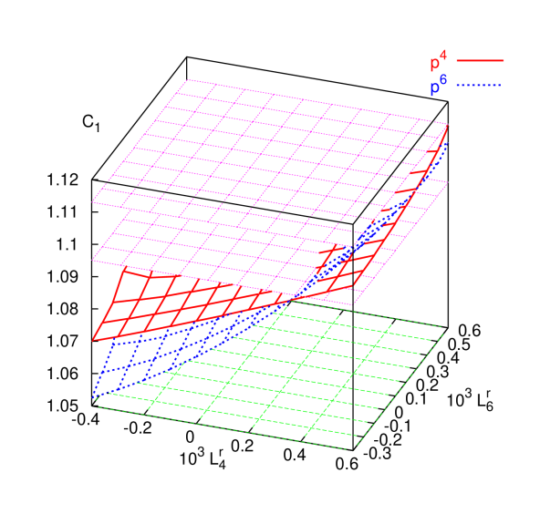
(a)

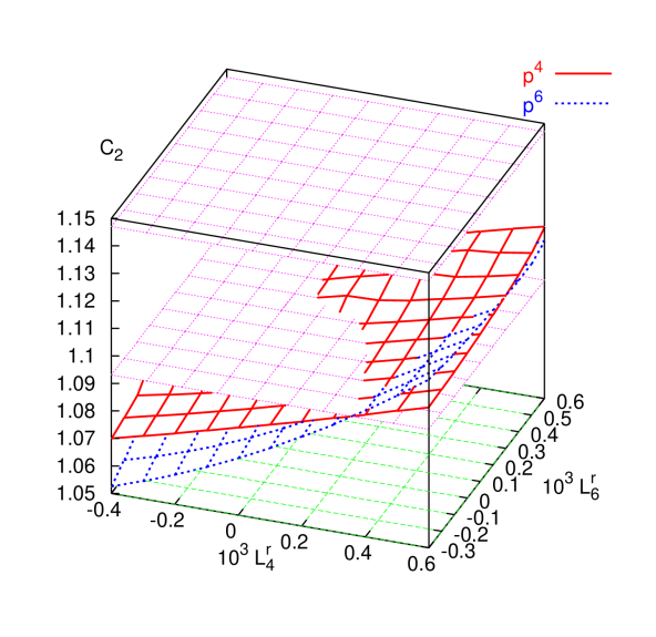
(b)

Figure 5: The subthreshold parameters $C_{1}$ and $C_{2}$ as a function of the input values $L_{4}^{r}$ and $L_{6}^{r}$ with the other $L_{i}^{r}$ simultaneously refitted to the $K_{e4}$ form factors. (a) $C_{1}$ calculated to order $p^{4}$ and $p^{6}$. (b) Idem for $C_{2}$. Notice that the lowest order value of 1 is outside the plotted region.

The plots show again that the preferred values of $L_{4}^{r}$ and $L_{6}^{r}$ are somewhat different from zero in order to obtain good agreement. The values of $c_{5}$ and $c_{6}$ can again be used to check the resonance predictions for two possible combinations of the $C_{i}^{r}$. These are in agreement to about a factor of two as expected. The values for $c_{3}$ is in good agreement with the one obtained by Ref. [21] but the $p^{6}$ contribution is of the opposite sign and larger than the $p^{4}$ contribution. For $c_{4}$ the agreement is marginal, similar to the one for $a^{0}_{2}$ shown in Table 2.

7 Conclusions

We have calculated $\pi\pi$ scattering to NNLO in three flavour ChPT and presented the full expressions in App. B. This is the main results of this work. We then presented a first numerical analysis and comparison with the low energy constants of order $p^{4}$ as determined from the absolute values of the form factors in $K_{e4}$.

This comparison led to the conclusion that the preferred values of $L_{4}^{r}$ and $L_{6}^{r}$ are somewhat different from zero but in size compatible with the error estimates based on the arguments from the large number of colours limit done in Ref. [6]. We have presented plots of two of the threshold parameters as a function of $L_{4}^{r}$ and $L_{6}^{r}$ with the other $L_{i}^{r}$ fitted to the $K_{e4}$ data. The values for the threshold parameters have been presented for fit 10 of Ref. [42] and fits A,B,C of Ref. [32]. The latter are those in the region preferred by the various scalar form factor constraints. The convergence of the three flavour ChPT series for $\pi\pi$ scattering seems reasonable and is similar to the one for the two flavour case after the masses and decay constants have been put to their physical values as was done here.

Appendix A Integrals

The one loop integrals we use are well known. The expressions for them can be found in [33] and [36]. The two loop integrals of sunset type were derived in [33] using the results of [51] for the subtraction constants. They are denoted by $\overline{H_{i}}$ in the expressions.

The two loop integrals of vertex type are evaluated using the methods of [52]. Their precise definition and method of evaluation can be found in [36]. They are denoted by $\overline{V}$ in the expressions.

Appendix B Analytical results

We now write the amplitude in the form (21) where we expand all functions in the ChPT expansion which we label by a superscript $(n)$ denoting the $p^{n}$ order in the expansion. The FORM files with this output will be made available in [53].

The lowest order result is [1]

$$V^{I(2)}(s)=0\,,\quad C(s,t,u)^{(2)}=-\frac{1}{F_{\pi}^{2}}\left(s-m_{\pi}^{2}\right)\,.$$ (35)

The order $p^{4}$ result agrees with the one shown in [10] and with the one in [9] up to a few misprints there. The result is

$$32\pi F_{\pi}^{4}\,V^{0(4)}(s) = +\overline{B}(m_{\pi}^{2},m_{\pi}^{2},s)\,\left(-2\,m_{\pi}^{2}\,s+1/2\,m_{\pi}^{4}+2\,s^{2}\right)$$

$$+\overline{B}(m_{K}^{2},m_{K}^{2},s)\,\left(3/8\,s^{2}\right)+\overline{B}(m_{\eta}^{2},m_{\eta}^{2},s)\,\left(1/6\,m_{\pi}^{4}\right)\,,$$

$$32\pi F_{\pi}^{4}\,V^{1(4)}(s) = +\overline{B}(m_{\pi}^{2},m_{\pi}^{2},s)\,\left(-2/9\,m_{\pi}^{2}+1/18\,s\right)$$

$$+\overline{B}(m_{K}^{2},m_{K}^{2},s)\,\left(-1/9\,m_{K}^{2}+1/36\,s\right)\,,$$

$$32\pi F_{\pi}^{4}\,V^{2(4)}(s) = +\overline{B}(m_{\pi}^{2},m_{\pi}^{2},s)\,\left(-2\,m_{\pi}^{2}\,s+1/2\,m_{\pi}^{4}+2\,s^{2}\right)$$ (36)

$$+\overline{B}(m_{K}^{2},m_{K}^{2},s)\,\left(3/8\,s^{2}\right)+\overline{B}(m_{\eta}^{2},m_{\eta}^{2},s)\,\left(1/6\,m_{\pi}^{4}\right)\,,$$

and for the polynomial part

$$C(s,t,u)^{(4)} = +\frac{1}{16\pi^{2}}\,\left(2/3\,m_{\pi}^{2}\,m_{K}^{2}-1/3\,m_{\pi}^{2}\,s+2/3\,m_{\pi}^{4}-1/2\,m_{K}^{2}\,s-1/8\,s^{2}+1/24\,\delta^{2}\right)$$ (37)

$$+\overline{A}(m_{\pi}^{2})\,\left(-4/3\,m_{\pi}^{2}+s\right)+\overline{A}(m_{K}^{2})\,\left(-2/3\,m_{\pi}^{2}+1/2\,s\right)$$

$$-32\,m_{\pi}^{2}\,L^{r}_{1}s-16\,m_{\pi}^{2}\,L^{r}_{3}s+16\,m_{\pi}^{2}\,L^{r}_{4}s+8\,m_{\pi}^{2}\,L^{r}_{5}s$$

$$+32\,m_{\pi}^{4}\,L^{r}_{1}+16\,m_{\pi}^{4}\,L^{r}_{3}-32\,m_{\pi}^{4}\,L^{r}_{4}-16\,m_{\pi}^{4}\,L^{r}_{5}$$

$$+32\,m_{\pi}^{4}\,L^{r}_{6}+16\,m_{\pi}^{4}\,L^{r}_{8}+8\,L^{r}_{1}s^{2}+2\,L^{r}_{2}s^{2}+2\,L^{r}_{2}\delta^{2}+4\,L^{r}_{3}s^{2}$$

Here we used the notation $\delta=t-u$ to have a shorter expression.

The order $p^{6}$ expressions are significantly longer. We split them in several parts

$$F_{\pi}^{6}\,C^{(6)}(s,t,u) = C_{\mathbf{C}}(s,t,u)+C_{\mathbf{L}}(s,t,u)+C_{\mathbf{6}}(s,t,u)\,,$$

$$32\pi F_{\pi}^{6}\,V^{I(6)}(s) = V^{I}_{\mathbf{L}}(s)+V^{I}_{\mathbf{6}}(s)+V^{I}_{\mathbf{V}}(s)\,.$$ (38)

The $C_{i}^{r}$ only contribute to the polynomial part.

$$C_{\mathbf{C}}(s,t,u) = +s\,\delta^{2}\,\left(+6\,C^{r}_{3}+2\,C^{r}_{4}\right)$$ (39)

$$+s\,\Big{(}-64\,m_{\pi}^{2}\,m_{K}^{2}\,C^{r}_{6}+64\,m_{\pi}^{2}\,m_{K}^{2}\,C^{r}_{11}-256\,m_{\pi}^{2}\,m_{K}^{2}\,C^{r}_{13}+32\,m_{\pi}^{2}\,m_{K}^{2}\,C^{r}_{15}$$

$$-96\,m_{\pi}^{4}\,C^{r}_{1}-192\,m_{\pi}^{4}\,C^{r}_{2}+96\,m_{\pi}^{4}\,C^{r}_{3}+32\,m_{\pi}^{4}\,C^{r}_{4}-32\,m_{\pi}^{4}\,C^{r}_{5}-32\,m_{\pi}^{4}\,C^{r}_{6}$$

$$-64\,m_{\pi}^{4}\,C^{r}_{7}-32\,m_{\pi}^{4}\,C^{r}_{8}+32\,m_{\pi}^{4}\,C^{r}_{10}+32\,m_{\pi}^{4}\,C^{r}_{11}-64\,m_{\pi}^{4}\,C^{r}_{12}$$

$$+32\,m_{\pi}^{4}\,C^{r}_{14}+48\,m_{\pi}^{4}\,C^{r}_{15}+64\,m_{\pi}^{4}\,C^{r}_{16}+32\,m_{\pi}^{4}\,C^{r}_{17}-32\,m_{\pi}^{4}\,C^{r}_{25}$$

$$+32\,m_{\pi}^{4}\,C^{r}_{26}+64\,m_{\pi}^{4}\,C^{r}_{28}-64\,m_{\pi}^{4}\,C^{r}_{29}-32\,m_{\pi}^{4}\,C^{r}_{30}\Big{)}$$

$$+s^{2}\,\Big{(}+48\,m_{\pi}^{2}\,C^{r}_{1}+96\,m_{\pi}^{2}\,C^{r}_{2}-48\,m_{\pi}^{2}\,C^{r}_{3}-40\,m_{\pi}^{2}\,C^{r}_{4}+8\,m_{\pi}^{2}\,C^{r}_{5}$$

$$+8\,m_{\pi}^{2}\,C^{r}_{6}+16\,m_{\pi}^{2}\,C^{r}_{7}+8\,m_{\pi}^{2}\,C^{r}_{8}-4\,m_{\pi}^{2}\,C^{r}_{10}-4\,m_{\pi}^{2}\,C^{r}_{11}+8\,m_{\pi}^{2}\,C^{r}_{12}$$

$$-8\,m_{\pi}^{2}\,C^{r}_{13}-8\,m_{\pi}^{2}\,C^{r}_{22}-8\,m_{\pi}^{2}\,C^{r}_{23}+20\,m_{\pi}^{2}\,C^{r}_{25}$$

$$+16\,m_{K}^{2}\,C^{r}_{6}-8\,m_{K}^{2}\,C^{r}_{11}+48\,m_{K}^{2}\,C^{r}_{13}\Big{)}$$

$$+s^{3}\,(-8\,C^{r}_{1}-16\,C^{r}_{2}+10\,C^{r}_{3}+14\,C^{r}_{4})$$

$$+\delta^{2}\,\Big{(}-8\,m_{\pi}^{2}\,C^{r}_{4}+4\,m_{\pi}^{2}\,C^{r}_{10}+4\,m_{\pi}^{2}\,C^{r}_{11}-8\,m_{\pi}^{2}\,C^{r}_{12}-8\,m_{\pi}^{2}\,C^{r}_{13}$$

$$+8\,m_{\pi}^{2}\,C^{r}_{22}+8\,m_{\pi}^{2}\,C^{r}_{23}-4\,m_{\pi}^{2}\,C^{r}_{25}+8\,m_{K}^{2}\,C^{r}_{11}-16\,m_{K}^{2}\,C^{r}_{13}\Big{)}$$

$$+64\,m_{\pi}^{4}\,m_{K}^{2}\,C^{r}_{6}-64\,m_{\pi}^{4}\,m_{K}^{2}\,C^{r}_{11}+192\,m_{\pi}^{4}\,m_{K}^{2}\,C^{r}_{13}-64\,m_{\pi}^{4}\,m_{K}^{2}\,C^{r}_{15}$$

$$+64\,m_{\pi}^{4}\,m_{K}^{2}\,C^{r}_{20}+384\,m_{\pi}^{4}\,m_{K}^{2}\,C^{r}_{21}+64\,m_{\pi}^{4}\,m_{K}^{2}\,C^{r}_{32}+64\,m_{\pi}^{6}\,C^{r}_{1}$$

$$+128\,m_{\pi}^{6}\,C^{r}_{2}-64\,m_{\pi}^{6}\,C^{r}_{3}+32\,m_{\pi}^{6}\,C^{r}_{5}+32\,m_{\pi}^{6}\,C^{r}_{6}+64\,m_{\pi}^{6}\,C^{r}_{7}+32\,m_{\pi}^{6}\,C^{r}_{8}$$

$$-32\,m_{\pi}^{6}\,C^{r}_{10}-32\,m_{\pi}^{6}\,C^{r}_{11}+32\,m_{\pi}^{6}\,C^{r}_{12}-32\,m_{\pi}^{6}\,C^{r}_{13}-64\,m_{\pi}^{6}\,C^{r}_{14}-96\,m_{\pi}^{6}\,C^{r}_{15}$$

$$-128\,m_{\pi}^{6}\,C^{r}_{16}-64\,m_{\pi}^{6}\,C^{r}_{17}+96\,m_{\pi}^{6}\,C^{r}_{19}+160\,m_{\pi}^{6}\,C^{r}_{20}+192\,m_{\pi}^{6}\,C^{r}_{21}$$

$$-64\,m_{\pi}^{6}\,C^{r}_{26}-128\,m_{\pi}^{6}\,C^{r}_{28}+64\,m_{\pi}^{6}\,C^{r}_{29}+96\,m_{\pi}^{6}\,C^{r}_{31}+160\,m_{\pi}^{6}\,C^{r}_{32}\,.$$

$$C_{\mathbf{L}}(s,t,u) = +\frac{1}{16\pi^{2}}\,\Big{(}+256/27\,m_{\pi}^{2}\,m_{K}^{2}\,L^{r}_{2}s+1048/81\,m_{\pi}^{2}\,m_{K}^{2}\,L^{r}_{3}s-8\,m_{\pi}^{2}\,m_{K}^{2}\,L^{r}_{5}s$$ (40)

$$-92/9\,m_{\pi}^{2}\,L^{r}_{1}s^{2}+28/9\,m_{\pi}^{2}\,L^{r}_{1}\delta^{2}-386/27\,m_{\pi}^{2}\,L^{r}_{2}s^{2}-2/9\,m_{\pi}^{2}\,L^{r}_{2}\delta^{2}$$

$$-320/81\,m_{\pi}^{2}\,L^{r}_{3}s^{2}+4/3\,m_{\pi}^{2}\,L^{r}_{3}\delta^{2}-8/3\,m_{\pi}^{2}\,L^{r}_{4}s^{2}+8/9\,m_{\pi}^{2}\,L^{r}_{4}\delta^{2}-2\,m_{\pi}^{2}\,L^{r}_{5}s^{2}$$

$$+2/3\,m_{\pi}^{2}\,L^{r}_{5}\delta^{2}+128/27\,m_{\pi}^{4}\,m_{K}^{2}\,L^{r}_{2}-736/81\,m_{\pi}^{4}\,m_{K}^{2}\,L^{r}_{3}+32/3\,m_{\pi}^{4}\,m_{K}^{2}\,L^{r}_{5}$$

$$+176/3\,m_{\pi}^{4}\,L^{r}_{1}s+808/27\,m_{\pi}^{4}\,L^{r}_{2}s+2008/81\,m_{\pi}^{4}\,L^{r}_{3}s-160/9\,m_{\pi}^{4}\,L^{r}_{4}s$$

$$-16/3\,m_{\pi}^{4}\,L^{r}_{5}s-448/9\,m_{\pi}^{6}\,L^{r}_{1}-224/27\,m_{\pi}^{6}\,L^{r}_{2}-1760/81\,m_{\pi}^{6}\,L^{r}_{3}$$

$$+256/9\,m_{\pi}^{6}\,L^{r}_{4}+32/3\,m_{\pi}^{6}\,L^{r}_{5}-8/3\,m_{K}^{2}\,L^{r}_{2}s^{2}-8/3\,m_{K}^{2}\,L^{r}_{3}s^{2}+2/3\,m_{K}^{2}\,L^{r}_{3}\delta^{2}$$

$$+1/9\,L^{r}_{1}s\,\delta^{2}+1/3\,L^{r}_{1}s^{3}+5/18\,L^{r}_{2}s\,\delta^{2}+13/6\,L^{r}_{2}s^{3}+1/9\,L^{r}_{3}s^{3}\Big{)}$$

$$+\overline{A}(m_{\eta}^{2})\,\Big{(}-16/3\,m_{\pi}^{2}\,L^{r}_{1}s-16/9\,m_{\pi}^{2}\,L^{r}_{2}s-40/27\,m_{\pi}^{2}\,L^{r}_{3}s+32/3\,m_{\pi}^{4}\,L^{r}_{1}$$

$$+16/9\,m_{\pi}^{4}\,L^{r}_{2}+64/27\,m_{\pi}^{4}\,L^{r}_{3}-16/3\,m_{\pi}^{4}\,L^{r}_{4}-8/9\,m_{\pi}^{4}\,L^{r}_{5}+32/3\,m_{\pi}^{4}\,L^{r}_{7}$$

$$+16/3\,m_{\pi}^{4}\,L^{r}_{8}\Big{)}$$

$$+\overline{A}(m_{\pi}^{2})\,\Big{(}-32/3\,m_{\pi}^{2}\,L^{r}_{1}s+184/3\,m_{\pi}^{2}\,L^{r}_{2}s-16/3\,m_{\pi}^{2}\,L^{r}_{3}s+64\,m_{\pi}^{2}\,L^{r}_{4}s$$

$$+32\,m_{\pi}^{2}\,L^{r}_{5}s+64\,m_{\pi}^{4}\,L^{r}_{1}-32\,m_{\pi}^{4}\,L^{r}_{2}+32\,m_{\pi}^{4}\,L^{r}_{3}-464/3\,m_{\pi}^{4}\,L^{r}_{4}$$

$$-232/3\,m_{\pi}^{4}\,L^{r}_{5}+160\,m_{\pi}^{4}\,L^{r}_{6}+80\,m_{\pi}^{4}\,L^{r}_{8}-12\,L^{r}_{1}s^{2}+4\,L^{r}_{1}\delta^{2}$$

$$-50/3\,L^{r}_{2}s^{2}+38/3\,L^{r}_{2}\delta^{2}-6\,L^{r}_{3}s^{2}+2\,L^{r}_{3}\delta^{2}\Big{)}$$

$$+\overline{A}(m_{K}^{2})\,\Big{(}-32\,m_{\pi}^{2}\,L^{r}_{1}s+16/3\,m_{\pi}^{2}\,L^{r}_{2}s-52/3\,m_{\pi}^{2}\,L^{r}_{3}s+16\,m_{\pi}^{2}\,L^{r}_{4}s$$

$$+16\,m_{\pi}^{2}\,L^{r}_{5}s+64\,m_{\pi}^{4}\,L^{r}_{1}+80/3\,m_{\pi}^{4}\,L^{r}_{3}-64\,m_{\pi}^{4}\,L^{r}_{4}-104/3\,m_{\pi}^{4}\,L^{r}_{5}$$

$$+64\,m_{\pi}^{4}\,L^{r}_{6}+32\,m_{\pi}^{4}\,L^{r}_{8}-4/3\,L^{r}_{2}s^{2}+4\,L^{r}_{2}\delta^{2}+5/3\,L^{r}_{3}s^{2}+1/3\,L^{r}_{3}\delta^{2}\Big{)}$$

$$+128\,m_{\pi}^{2}\,m_{K}^{2}\,L^{r}_{4}L^{r}_{5}s-512\,m_{\pi}^{2}\,m_{K}^{2}\,L^{r}_{4}L^{r}_{6}s+256\,m_{\pi}^{2}\,m_{K}^{2}\,(L^{r}_{4})^{2}\,s$$

$$-256\,m_{\pi}^{2}\,m_{K}^{2}\,L^{r}_{5}L^{r}_{6}s-256\,m_{\pi}^{4}\,m_{K}^{2}\,L^{r}_{4}L^{r}_{5}+2048\,m_{\pi}^{4}\,m_{K}^{2}\,L^{r}_{4}L^{r}_{6}$$

$$+512\,m_{\pi}^{4}\,m_{K}^{2}\,L^{r}_{4}L^{r}_{8}-512\,m_{\pi}^{4}\,m_{K}^{2}\,(L^{r}_{4})^{2}+512\,m_{\pi}^{4}\,m_{K}^{2}\,L^{r}_{5}L^{r}_{6}$$

$$-1024\,m_{\pi}^{4}\,m_{K}^{2}\,L^{r}_{6}L^{r}_{8}-2048\,m_{\pi}^{4}\,m_{K}^{2}\,(L^{r}_{6})^{2}+192\,m_{\pi}^{4}\,L^{r}_{4}L^{r}_{5}s$$

$$-256\,m_{\pi}^{4}\,L^{r}_{4}L^{r}_{6}s-256\,m_{\pi}^{4}\,L^{r}_{4}L^{r}_{8}s+128\,m_{\pi}^{4}\,(L^{r}_{4})^{2}\,s-128\,m_{\pi}^{4}\,L^{r}_{5}L^{r}_{6}s$$

$$-128\,m_{\pi}^{4}\,L^{r}_{5}L^{r}_{8}s+64\,m_{\pi}^{4}\,(L^{r}_{5})^{2}\,s-384\,m_{\pi}^{6}\,L^{r}_{4}L^{r}_{5}+1024\,m_{\pi}^{6}\,L^{r}_{4}L^{r}_{6}$$

$$+768\,m_{\pi}^{6}\,L^{r}_{4}L^{r}_{8}-256\,m_{\pi}^{6}\,(L^{r}_{4})^{2}+768\,m_{\pi}^{6}\,L^{r}_{5}L^{r}_{6}+512\,m_{\pi}^{6}\,L^{r}_{5}L^{r}_{8}$$

$$-128\,m_{\pi}^{6}\,(L^{r}_{5})^{2}-1536\,m_{\pi}^{6}\,L^{r}_{6}L^{r}_{8}-1024\,m_{\pi}^{6}\,(L^{r}_{6})^{2}-512\,m_{\pi}^{6}\,(L^{r}_{8})^{2}\,.$$

$$C_{\mathbf{6}}(s,t,u) = +\frac{1}{16\pi^{2}}\,\overline{A}(m_{\eta}^{2})\,\Big{(}+1/36\,m_{\pi}^{2}\,s-1/9\,m_{\pi}^{4}\Big{)}$$ (41)

$$+\frac{1}{16\pi^{2}}\,\overline{A}(m_{\pi}^{2})\,\Big{(}+8/9\,m_{\pi}^{2}\,m_{K}^{2}-89/36\,m_{\pi}^{2}\,s+29/18\,m_{\pi}^{4}-2/3\,m_{K}^{2}\,s$$

$$+5/24\,s^{2}-1/72\,\delta^{2}\Big{)}$$

$$+\frac{1}{16\pi^{2}}\,\overline{A}(m_{K}^{2})\,\Big{(}+4/9\,m_{\pi}^{2}\,m_{K}^{2}-37/36\,m_{\pi}^{2}\,s+3/4\,m_{\pi}^{4}-1/3\,m_{K}^{2}\,s$$

$$+1/24\,s^{2}+1/72\,\delta^{2}\Big{)}$$

$$+\left(\frac{1}{16\pi^{2}}\right)^{2}\,\Big{(}-83/216\,m_{\pi}^{2}\,m_{K}^{2}\,pi^{2}\,s-1375/432\,m_{\pi}^{2}\,m_{K}^{2}\,s-2/9\,m_{\pi}^{2}\,m_{K}^{4}$$

$$+13/32\,m_{\pi}^{2}\,\pi^{2}\,s^{2}-19/288\,m_{\pi}^{2}\,pi^{2}\,\delta^{2}+1751/432\,m_{\pi}^{2}\,s^{2}-289/432\,m_{\pi}^{2}\,\delta^{2}$$

$$+103/648\,m_{\pi}^{4}\,m_{K}^{2}\,\pi^{2}+167/432\,m_{\pi}^{4}\,m_{K}^{2}-337/216\,m_{\pi}^{4}\,\pi^{2}\,s$$

$$-10933/864\,m_{\pi}^{4}\,s+349/324\,m_{\pi}^{6}\,\pi^{2}+6013/864\,m_{\pi}^{6}+1/8\,m_{K}^{2}\,\pi^{2}\,s^{2}$$

$$-1/144\,m_{K}^{2}\,\pi^{2}\,\delta^{2}+13/12\,m_{K}^{2}\,s^{2}-7/72\,m_{K}^{2}\,\delta^{2}+1/6\,m_{K}^{4}\,s$$

$$-1/96\,s\,\delta^{2}-11/96\,s^{3}\Big{)}$$

$$+\overline{A}(m_{\eta}^{2})^{2}\,\Big{(}+1/12\,m_{\pi}^{2}\,m_{\eta}^{-2}\,s-2/9\,m_{\pi}^{4}\,m_{\eta}^{-2}\Big{)}$$

$$+\overline{A}(m_{\pi}^{2})\,\overline{A}(m_{K}^{2})\,\Big{(}-8/9\,m_{\pi}^{2}+2/3\,s\Big{)}$$

$$+\overline{A}(m_{\pi}^{2})^{2}\,\Big{(}+39/16\,m_{\pi}^{-2}\,s^{2}-19/48\,m_{\pi}^{-2}\,\delta^{2}+11/2\,m_{\pi}^{2}-26/3\,s\Big{)}$$

$$+\overline{A}(m_{K}^{2})^{2}\,\Big{(}-29/12\,m_{\pi}^{2}\,m_{K}^{-2}\,s-2/9\,m_{\pi}^{2}+5/4\,m_{\pi}^{4}\,m_{K}^{-2}+3/4\,m_{K}^{-2}\,s^{2}$$

$$-1/24\,m_{K}^{-2}\,\delta^{2}+1/6\,s\Big{)}$$

$$+H^{F\prime}(m_{\pi}^{2},m_{\pi}^{2},m_{\pi}^{2},m_{\pi}^{2})\,\Big{(}+5/2\,m_{\pi}^{4}\,s-5/2\,m_{\pi}^{6}\Big{)}$$

$$+H^{F\prime}(m_{\pi}^{2},m_{K}^{2},m_{K}^{2},m_{\pi}^{2})\,\Big{(}-15/8\,m_{\pi}^{4}\,s+15/8\,m_{\pi}^{6}\Big{)}$$

$$+H^{F\prime}(m_{\pi}^{2},m_{\eta}^{2},m_{\eta}^{2},m_{\pi}^{2})\,\Big{(}+1/6\,m_{\pi}^{4}\,s-1/6\,m_{\pi}^{6}\Big{)}$$

$$+H^{F\prime}(m_{K}^{2},m_{\pi}^{2},m_{K}^{2},m_{\pi}^{2})\,\Big{(}+3\,m_{\pi}^{2}\,m_{K}^{2}\,s-3\,m_{\pi}^{4}\,m_{K}^{2}\Big{)}$$

$$+H^{F\prime}(m_{K}^{2},m_{K}^{2},m_{\eta}^{2},m_{\pi}^{2})\,\Big{(}-5/2\,m_{\pi}^{4}\,s+5/2\,m_{\pi}^{6}\Big{)}$$

$$+H^{F\prime}(m_{\eta}^{2},m_{K}^{2},m_{K}^{2},m_{\pi}^{2})\,\Big{(}+3/2\,m_{\pi}^{2}\,m_{K}^{2}\,s-3/2\,m_{\pi}^{4}\,m_{K}^{2}+13/8\,m_{\pi}^{4}\,s$$

$$-13/8\,m_{\pi}^{6}\Big{)}$$

$$+H^{F\prime}_{1}(m_{\pi}^{2},m_{K}^{2},m_{K}^{2},m_{\pi}^{2})\,\Big{(}+3\,m_{\pi}^{4}\,s-3\,m_{\pi}^{6}\Big{)}$$

$$+H^{F\prime}_{1}(m_{K}^{2},m_{K}^{2},m_{\eta}^{2},m_{\pi}^{2})\,\Big{(}+2\,m_{\pi}^{4}\,s-2\,m_{\pi}^{6}\Big{)}$$

$$+H^{F\prime}_{1}(m_{\eta}^{2},m_{K}^{2},m_{K}^{2},m_{\pi}^{2})\,\Big{(}-2\,m_{\pi}^{4}\,s+2\,m_{\pi}^{6}\Big{)}$$

$$+H^{F\prime}_{21}(m_{\pi}^{2},m_{\pi}^{2},m_{\pi}^{2},m_{\pi}^{2})\,\Big{(}+9\,m_{\pi}^{4}\,s-9\,m_{\pi}^{6}\Big{)}$$

$$+H^{F\prime}_{21}(m_{\pi}^{2},m_{K}^{2},m_{K}^{2},m_{\pi}^{2})\,\Big{(}-9/8\,m_{\pi}^{4}\,s+9/8\,m_{\pi}^{6}\Big{)}$$

$$+H^{F\prime}_{21}(m_{K}^{2},m_{\pi}^{2},m_{K}^{2},m_{\pi}^{2})\,\Big{(}+9\,m_{\pi}^{4}\,s-9\,m_{\pi}^{6}\Big{)}$$

$$+H^{F\prime}_{21}(m_{\eta}^{2},m_{K}^{2},m_{K}^{2},m_{\pi}^{2})\,\Big{(}+27/8\,m_{\pi}^{4}\,s-27/8\,m_{\pi}^{6}\Big{)}$$

$$+H^{F}(m_{\pi}^{2},m_{\pi}^{2},m_{\pi}^{2},m_{\pi}^{2})\,\Big{(}+4\,m_{\pi}^{2}\,s-17/6\,m_{\pi}^{4}-s^{2}+1/3\,\delta^{2}\Big{)}$$

$$+H^{F}(m_{\pi}^{2},m_{K}^{2},m_{K}^{2},m_{\pi}^{2})\,\Big{(}-133/36\,m_{\pi}^{2}\,s+10/3\,m_{\pi}^{4}-5/16\,s^{2}+7/16\,\delta^{2}\Big{)}$$

$$+H^{F}(m_{\pi}^{2},m_{\eta}^{2},m_{\eta}^{2},m_{\pi}^{2})\,\Big{(}+1/18\,m_{\pi}^{4}\Big{)}$$

$$+H^{F}(m_{K}^{2},m_{\pi}^{2},m_{K}^{2},m_{\pi}^{2})\,\Big{(}-1/12\,m_{\pi}^{2}\,m_{K}^{2}+53/18\,m_{\pi}^{2}\,s-4/3\,m_{\pi}^{4}$$

$$+13/72\,m_{K}^{2}\,s-1/4\,s^{2}-1/4\,\delta^{2}\Big{)}$$

$$+H^{F}(m_{K}^{2},m_{K}^{2},m_{\pi}^{2},m_{\pi}^{2})\,\Big{(}+1/12\,m_{\pi}^{2}\,m_{K}^{2}-13/72\,m_{K}^{2}\,s\Big{)}$$

$$+H^{F}(m_{K}^{2},m_{K}^{2},m_{\eta}^{2},m_{\pi}^{2})\,\Big{(}-7/18\,m_{\pi}^{4}+3/16\,s^{2}-3/16\,\delta^{2}\Big{)}$$

$$+H^{F}(m_{\eta}^{2},m_{K}^{2},m_{K}^{2},m_{\pi}^{2})\,\Big{(}-11/8\,m_{\pi}^{2}\,s+119/36\,m_{\pi}^{4}-45/64\,s^{2}+27/64\,\delta^{2}\Big{)}$$

$$+H^{F}_{1}(m_{\pi}^{2},m_{K}^{2},m_{K}^{2},m_{\pi}^{2})\,\Big{(}+7/4\,m_{\pi}^{2}\,s-3/2\,m_{\pi}^{4}-3/16\,s^{2}+1/16\,\delta^{2}\Big{)}$$

$$+H^{F}_{1}(m_{\eta}^{2},m_{K}^{2},m_{K}^{2},m_{\pi}^{2})\,\Big{(}+11/8\,m_{\pi}^{2}\,s-15/4\,m_{\pi}^{4}+45/64\,s^{2}-27/64\,\delta^{2}\Big{)}$$

$$+H^{F}_{21}(m_{\pi}^{2},m_{\pi}^{2},m_{\pi}^{2},m_{\pi}^{2})\,\Big{(}+5\,m_{\pi}^{2}\,s-m_{\pi}^{4}-3/2\,s^{2}+1/2\,\delta^{2}\Big{)}$$

$$+H^{F}_{21}(m_{\pi}^{2},m_{K}^{2},m_{K}^{2},m_{\pi}^{2})\,\Big{(}-13/8\,m_{\pi}^{2}\,s+1/8\,m_{\pi}^{4}+15/16\,s^{2}-5/16\,\delta^{2}\Big{)}$$

$$+H^{F}_{21}(m_{K}^{2},m_{\pi}^{2},m_{K}^{2},m_{\pi}^{2})\,\Big{(}+253/24\,m_{\pi}^{2}\,s-45/4\,m_{\pi}^{4}+3/8\,s^{2}-1/8\,\delta^{2}\Big{)}$$

$$+H^{F}_{21}(m_{K}^{2},m_{K}^{2},m_{\pi}^{2},m_{\pi}^{2})\,\Big{(}-37/24\,m_{\pi}^{2}\,s+17/4\,m_{\pi}^{4}-3/2\,s^{2}+1/2\,\delta^{2}\Big{)}$$

$$+H^{F}_{21}(m_{K}^{2},m_{K}^{2},m_{\eta}^{2},m_{\pi}^{2})\,\Big{(}+3/2\,m_{\pi}^{2}\,s-9/2\,m_{\pi}^{4}+45/32\,s^{2}-15/32\,\delta^{2}\Big{)}$$

$$+H^{F}_{21}(m_{\eta}^{2},m_{K}^{2},m_{K}^{2},m_{\pi}^{2})\,\Big{(}+21/8\,m_{\pi}^{2}\,s-3/8\,m_{\pi}^{4}-9/8\,s^{2}+3/8\,\delta^{2}\Big{)}\,.$$

$$V^{0}_{\mathbf{L}}(s) = +\overline{B}(m_{\pi}^{2},m_{\pi}^{2},s)\,\Big{(}-728/3\,m_{\pi}^{2}\,L^{r}_{1}s^{2}-376/3\,m_{\pi}^{2}\,L^{r}_{2}s^{2}-364/3\,m_{\pi}^{2}\,L^{r}_{3}s^{2}$$ (42)

$$+64\,m_{\pi}^{2}\,L^{r}_{4}s^{2}+32\,m_{\pi}^{2}\,L^{r}_{5}s^{2}+1024/3\,m_{\pi}^{4}\,L^{r}_{1}s+608/3\,m_{\pi}^{4}\,L^{r}_{2}s+512/3\,m_{\pi}^{4}\,L^{r}_{3}s$$

$$-224\,m_{\pi}^{4}\,L^{r}_{4}s-112\,m_{\pi}^{4}\,L^{r}_{5}s+320\,m_{\pi}^{4}\,L^{r}_{6}s+160\,m_{\pi}^{4}\,L^{r}_{8}s-352/3\,m_{\pi}^{6}\,L^{r}_{1}$$

$$-224/3\,m_{\pi}^{6}\,L^{r}_{2}-176/3\,m_{\pi}^{6}\,L^{r}_{3}+96\,m_{\pi}^{6}\,L^{r}_{4}+48\,m_{\pi}^{6}\,L^{r}_{5}-160\,m_{\pi}^{6}\,L^{r}_{6}$$

$$-80\,m_{\pi}^{6}\,L^{r}_{8}+176/3\,L^{r}_{1}s^{3}+112/3\,L^{r}_{2}s^{3}+88/3\,L^{r}_{3}s^{3}\Big{)}$$

$$+\overline{B}(m_{K}^{2},m_{K}^{2},s)\,\Big{(}+96\,m_{\pi}^{2}\,m_{K}^{2}\,L^{r}_{1}s+32\,m_{\pi}^{2}\,m_{K}^{2}\,L^{r}_{2}s+32\,m_{\pi}^{2}\,m_{K}^{2}\,L^{r}_{3}s$$

$$-96\,m_{\pi}^{2}\,m_{K}^{2}\,L^{r}_{4}s-24\,m_{\pi}^{2}\,m_{K}^{2}\,L^{r}_{5}s+96\,m_{\pi}^{2}\,m_{K}^{2}\,L^{r}_{6}s+48\,m_{\pi}^{2}\,m_{K}^{2}\,L^{r}_{8}s$$

$$-48\,m_{\pi}^{2}\,L^{r}_{1}s^{2}-8\,m_{\pi}^{2}\,L^{r}_{2}s^{2}-14\,m_{\pi}^{2}\,L^{r}_{3}s^{2}+24\,m_{\pi}^{2}\,L^{r}_{4}s^{2}+6\,m_{\pi}^{2}\,L^{r}_{5}s^{2}$$

$$-48\,m_{K}^{2}\,L^{r}_{1}s^{2}-8\,m_{K}^{2}\,L^{r}_{2}s^{2}-14\,m_{K}^{2}\,L^{r}_{3}s^{2}+24\,m_{K}^{2}\,L^{r}_{4}s^{2}+24\,L^{r}_{1}s^{3}$$

$$+8\,L^{r}_{2}s^{3}+8\,L^{r}_{3}s^{3}\Big{)}$$

$$+\overline{B}(m_{\eta}^{2},m_{\eta}^{2},s)\,\Big{(}-64/3\,m_{\pi}^{2}\,m_{K}^{2}\,L^{r}_{1}s-32/9\,m_{\pi}^{2}\,m_{K}^{2}\,L^{r}_{2}s-128/27\,m_{\pi}^{2}\,m_{K}^{2}\,L^{r}_{3}s$$

$$+32/3\,m_{\pi}^{2}\,m_{K}^{2}\,L^{r}_{4}s+8\,m_{\pi}^{2}\,L^{r}_{1}s^{2}+8/3\,m_{\pi}^{2}\,L^{r}_{2}s^{2}+20/9\,m_{\pi}^{2}\,L^{r}_{3}s^{2}$$

$$+128/3\,m_{\pi}^{4}\,m_{K}^{2}\,L^{r}_{1}+128/9\,m_{\pi}^{4}\,m_{K}^{2}\,L^{r}_{2}+320/27\,m_{\pi}^{4}\,m_{K}^{2}\,L^{r}_{3}-128/3\,m_{\pi}^{4}\,m_{K}^{2}\,L^{r}_{4}$$

$$-64/9\,m_{\pi}^{4}\,m_{K}^{2}\,L^{r}_{5}+128/3\,m_{\pi}^{4}\,m_{K}^{2}\,L^{r}_{6}-128/3\,m_{\pi}^{4}\,m_{K}^{2}\,L^{r}_{7}-32/3\,m_{\pi}^{4}\,L^{r}_{1}s$$

$$-16/9\,m_{\pi}^{4}\,L^{r}_{2}s-64/27\,m_{\pi}^{4}\,L^{r}_{3}s+16/3\,m_{\pi}^{4}\,L^{r}_{4}s-32/3\,m_{\pi}^{6}\,L^{r}_{1}-32/9\,m_{\pi}^{6}\,L^{r}_{2}$$

$$-80/27\,m_{\pi}^{6}\,L^{r}_{3}+32/3\,m_{\pi}^{6}\,L^{r}_{4}+16/9\,m_{\pi}^{6}\,L^{r}_{5}-32/3\,m_{\pi}^{6}\,L^{r}_{6}+128/3\,m_{\pi}^{6}\,L^{r}_{7}$$

$$+16\,m_{\pi}^{6}\,L^{r}_{8}\Big{)}\,.$$

$$V^{0}_{\mathbf{6}}(s) = +\overline{B}(m_{\pi}^{2},m_{\pi}^{2},s)\,\frac{1}{16\pi^{2}}\,\Big{(}+85/24\,m_{\pi}^{2}\,s^{2}-25/3\,m_{\pi}^{4}\,s+10/3\,m_{\pi}^{6}-5/12\,s^{3}\Big{)}$$ (43)

$$+\overline{B}(m_{\pi}^{2},m_{\pi}^{2},s)^{2}\,\Big{(}-3\,m_{\pi}^{2}\,s^{2}+3/2\,m_{\pi}^{4}\,s-1/4\,m_{\pi}^{6}+2\,s^{3}\Big{)}$$

$$+\overline{B}(m_{\pi}^{2},m_{\pi}^{2},s)\,\overline{B}(m_{K}^{2},m_{K}^{2},s)\,\Big{(}-3/8\,m_{\pi}^{2}\,s^{2}+3/4\,s^{3}\Big{)}$$

$$+\overline{B}(m_{\pi}^{2},m_{\pi}^{2},s)\,\overline{B}(m_{\eta}^{2},m_{\eta}^{2},s)\,\Big{(}+1/3\,m_{\pi}^{4}\,s-1/6\,m_{\pi}^{6}\Big{)}$$

$$+\overline{B}(m_{\pi}^{2},m_{\pi}^{2},s)\,\Big{(}-20\,m_{\pi}^{2}\,s\,\overline{A}(m_{\pi}^{2})-10\,m_{\pi}^{2}\,s\,\overline{A}(m_{K}^{2})+8\,m_{\pi}^{4}\,\overline{A}(m_{\pi}^{2})$$

$$+4\,m_{\pi}^{4}\,\overline{A}(m_{K}^{2})+8\,s^{2}\,\overline{A}(m_{\pi}^{2})+4\,s^{2}\,\overline{A}(m_{K}^{2})\Big{)}$$

$$+\overline{B}(m_{K}^{2},m_{K}^{2},s)\,\frac{1}{16\pi^{2}}\,\Big{(}-2\,m_{\pi}^{2}\,m_{K}^{2}\,s+1/2\,m_{\pi}^{2}\,s^{2}+1/2\,m_{K}^{2}\,s^{2}-1/8\,s^{3}\Big{)}$$

$$+\overline{B}(m_{K}^{2},m_{K}^{2},s)^{2}\,\Big{(}+9/32\,s^{3}\Big{)}$$

$$+\overline{B}(m_{K}^{2},m_{K}^{2},s)\,\overline{B}(m_{\eta}^{2},m_{\eta}^{2},s)\,\Big{(}$$

$$-1/3\,m_{\pi}^{2}\,m_{K}^{2}\,s+3/8\,m_{\pi}^{2}\,s^{2}\Big{)}$$

$$+\overline{B}(m_{K}^{2},m_{K}^{2},s)\,\Big{(}-3/4\,m_{\pi}^{2}\,\overline{A}(m_{\eta}^{2})\,s-9/4\,m_{\pi}^{2}\,s\,\overline{A}(m_{\pi}^{2})-3/2\,m_{\pi}^{2}\,s\,\overline{A}(m_{K}^{2})$$

$$+3/2\,s^{2}\,\overline{A}(m_{\pi}^{2})+3/4\,s^{2}\,\overline{A}(m_{K}^{2})\Big{)}$$

$$+\overline{B}(m_{\eta}^{2},m_{\eta}^{2},s)\,\frac{1}{16\pi^{2}}\,\Big{(}+2/9\,m_{\pi}^{2}\,m_{K}^{2}\,s-1/24\,m_{\pi}^{2}\,s^{2}-8/9\,m_{\pi}^{4}\,m_{K}^{2}+1/9\,m_{\pi}^{4}\,s$$

$$+2/9\,m_{\pi}^{6}\Big{)}$$

$$+\overline{B}(m_{\eta}^{2},m_{\eta}^{2},s)^{2}\,\Big{(}+4/27\,m_{\pi}^{4}\,m_{K}^{2}-7/108\,m_{\pi}^{6}\Big{)}$$

$$+\overline{B}(m_{\eta}^{2},m_{\eta}^{2},s)\,\Big{(}+2/3\,m_{\pi}^{4}\,\overline{A}(m_{\pi}^{2})-2/3\,m_{\pi}^{4}\,\overline{A}(m_{K}^{2})\Big{)}$$

$$+\overline{B}^{\epsilon}(m_{\pi}^{2},m_{\pi}^{2},s)\,\frac{1}{16\pi^{2}}\,\Big{(}-10\,m_{\pi}^{2}\,m_{K}^{2}\,s+59/4\,m_{\pi}^{2}\,s^{2}+4\,m_{\pi}^{4}\,m_{K}^{2}$$

$$-335/9\,m_{\pi}^{4}\,s+136/9\,m_{\pi}^{6}+4\,m_{K}^{2}\,s^{2}-3/2\,s^{3}\Big{)}$$

$$+\overline{B}^{\epsilon}(m_{K}^{2},m_{K}^{2},s)\,\frac{1}{16\pi^{2}}\,\Big{(}-6\,m_{\pi}^{2}\,m_{K}^{2}\,s+15/8\,m_{\pi}^{2}\,s^{2}-2\,m_{\pi}^{4}\,s+9/4\,m_{K}^{2}\,s^{2}$$

$$-9/16\,s^{3}\Big{)}$$

$$+\overline{B}^{\epsilon}(m_{\eta}^{2},m_{\eta}^{2},s)\,\frac{1}{16\pi^{2}}\,\Big{(}+1/3\,m_{\pi}^{2}\,m_{K}^{2}\,s-1/4\,m_{\pi}^{2}\,s^{2}-4/3\,m_{\pi}^{4}\,m_{K}^{2}+2/3\,m_{\pi}^{4}\,s$$

$$-2/9\,m_{\pi}^{6}\Big{)}\,.$$

$$V^{0}_{\mathbf{V}}(s) = +V_{0}(m_{\pi}^{2},m_{\pi}^{2},m_{\pi}^{2},m_{\pi}^{2},m_{\pi}^{2},s,m_{\pi}^{2})\,\Big{(}+4\,m_{\pi}^{2}\,s^{2}-4\,m_{\pi}^{4}\,s+m_{\pi}^{6}\Big{)}$$ (44)

$$+V_{0}(m_{\pi}^{2},m_{\pi}^{2},m_{K}^{2},m_{K}^{2},m_{\pi}^{2},s,m_{\pi}^{2})\,\Big{(}+1/2\,m_{\pi}^{2}\,s^{2}-9/4\,m_{\pi}^{4}\,s+m_{\pi}^{6}\Big{)}$$

$$+V_{0}(m_{\pi}^{2},m_{\pi}^{2},m_{\eta}^{2},m_{\eta}^{2},m_{\pi}^{2},s,m_{\pi}^{2})\,\Big{(}+2/9\,m_{\pi}^{4}\,s-1/9\,m_{\pi}^{6}\Big{)}$$

$$+V_{0}(m_{K}^{2},m_{K}^{2},m_{\pi}^{2},m_{K}^{2},m_{\pi}^{2},s,m_{\pi}^{2})\,\Big{(}+9/2\,m_{\pi}^{4}\,s\Big{)}$$

$$+V_{0}(m_{K}^{2},m_{K}^{2},m_{K}^{2},m_{\eta}^{2},m_{\pi}^{2},s,m_{\pi}^{2})\,\Big{(}-3/8\,m_{\pi}^{2}\,s^{2}+2\,m_{\pi}^{4}\,s\Big{)}$$

$$+V_{0}(m_{\eta}^{2},m_{\eta}^{2},m_{\pi}^{2},m_{\eta}^{2},m_{\pi}^{2},s,m_{\pi}^{2})\,\Big{(}+2/9\,m_{\pi}^{6}\Big{)}$$

$$+V_{0}(m_{\eta}^{2},m_{\eta}^{2},m_{K}^{2},m_{K}^{2},m_{\pi}^{2},s,m_{\pi}^{2})\,\Big{(}+1/4\,m_{\pi}^{4}\,s+1/3\,m_{\pi}^{6}\Big{)}$$

$$+V_{11}(m_{\pi}^{2},m_{\pi}^{2},m_{K}^{2},m_{K}^{2},m_{\pi}^{2},s,m_{\pi}^{2})\,\Big{(}-m_{\pi}^{2}\,s^{2}+9/2\,m_{\pi}^{4}\,s-2\,m_{\pi}^{6}\Big{)}$$

$$+V_{11}(m_{K}^{2},m_{K}^{2},m_{\pi}^{2},m_{K}^{2},m_{\pi}^{2},s,m_{\pi}^{2})\,\Big{(}+3\,m_{\pi}^{2}\,s^{2}-12\,m_{\pi}^{4}\,s\Big{)}$$

$$+V_{11}(m_{K}^{2},m_{K}^{2},m_{K}^{2},m_{\eta}^{2},m_{\pi}^{2},s,m_{\pi}^{2})\,\Big{(}+3/2\,m_{\pi}^{2}\,s^{2}-6\,m_{\pi}^{4}\,s\Big{)}$$

$$+V_{11}(m_{\eta}^{2},m_{\eta}^{2},m_{K}^{2},m_{K}^{2},m_{\pi}^{2},s,m_{\pi}^{2})\,\Big{(}+1/2\,m_{\pi}^{4}\,s-2\,m_{\pi}^{6}\Big{)}$$

$$+V_{13}(m_{K}^{2},m_{K}^{2},m_{\pi}^{2},m_{K}^{2},m_{\pi}^{2},s,m_{\pi}^{2})\,\Big{(}+21/4\,m_{\pi}^{2}\,s^{2}-9\,m_{\pi}^{4}\,s-3/4\,s^{3}\Big{)}$$

$$+V_{13}(m_{K}^{2},m_{K}^{2},m_{K}^{2},m_{\eta}^{2},m_{\pi}^{2},s,m_{\pi}^{2})\,\Big{(}+15/4\,m_{\pi}^{2}\,s^{2}-6\,m_{\pi}^{4}\,s-9/16\,s^{3}\Big{)}$$

$$+V_{14}(m_{K}^{2},m_{K}^{2},m_{\pi}^{2},m_{K}^{2},m_{\pi}^{2},s,m_{\pi}^{2})\,\Big{(}+6\,m_{\pi}^{2}\,s^{2}-3/2\,s^{3}\Big{)}$$

$$+V_{14}(m_{K}^{2},m_{K}^{2},m_{K}^{2},m_{\eta}^{2},m_{\pi}^{2},s,m_{\pi}^{2})\,\Big{(}+9/2\,m_{\pi}^{2}\,s^{2}-9/8\,s^{3}\Big{)}$$

$$+V_{22}(m_{\pi}^{2},m_{\pi}^{2},m_{\pi}^{2},m_{\pi}^{2},m_{\pi}^{2},s,m_{\pi}^{2})\,\Big{(}-4\,m_{\pi}^{2}\,s^{2}+18\,m_{\pi}^{4}\,s-8\,m_{\pi}^{6}\Big{)}$$

$$+V_{22}(m_{\pi}^{2},m_{\pi}^{2},m_{K}^{2},m_{K}^{2},m_{\pi}^{2},s,m_{\pi}^{2})\,\Big{(}+1/2\,m_{\pi}^{2}\,s^{2}-9/4\,m_{\pi}^{4}\,s+m_{\pi}^{6}\Big{)}$$

$$+V_{22}(m_{K}^{2},m_{K}^{2},m_{\pi}^{2},m_{K}^{2},m_{\pi}^{2},s,m_{\pi}^{2})\,\Big{(}-3\,m_{\pi}^{2}\,s^{2}+12\,m_{\pi}^{4}\,s\Big{)}$$

$$+V_{22}(m_{K}^{2},m_{K}^{2},m_{K}^{2},m_{\eta}^{2},m_{\pi}^{2},s,m_{\pi}^{2})\,\Big{(}-9/8\,m_{\pi}^{2}\,s^{2}+9/2\,m_{\pi}^{4}\,s\Big{)}$$

$$+V_{22}(m_{\eta}^{2},m_{\eta}^{2},m_{K}^{2},m_{K}^{2},m_{\pi}^{2},s,m_{\pi}^{2})\,\Big{(}-3/4\,m_{\pi}^{4}\,s+3\,m_{\pi}^{6}\Big{)}$$

$$+V_{23}(m_{\pi}^{2},m_{\pi}^{2},m_{\pi}^{2},m_{\pi}^{2},m_{\pi}^{2},s,m_{\pi}^{2})\,\Big{(}-18\,m_{\pi}^{2}\,s^{2}+8\,m_{\pi}^{4}\,s+4\,s^{3}\Big{)}$$

$$+V_{23}(m_{\pi}^{2},m_{\pi}^{2},m_{K}^{2},m_{K}^{2},m_{\pi}^{2},s,m_{\pi}^{2})\,\Big{(}+9/4\,m_{\pi}^{2}\,s^{2}-m_{\pi}^{4}\,s-1/2\,s^{3}\Big{)}$$

$$+V_{23}(m_{K}^{2},m_{K}^{2},m_{\pi}^{2},m_{K}^{2},m_{\pi}^{2},s,m_{\pi}^{2})\,\Big{(}-12\,m_{\pi}^{2}\,s^{2}+3\,s^{3}\Big{)}$$

$$+V_{23}(m_{K}^{2},m_{K}^{2},m_{K}^{2},m_{\eta}^{2},m_{\pi}^{2},s,m_{\pi}^{2})\,\Big{(}-9/2\,m_{\pi}^{2}\,s^{2}+9/8\,s^{3}\Big{)}$$

$$+V_{23}(m_{\eta}^{2},m_{\eta}^{2},m_{K}^{2},m_{K}^{2},m_{\pi}^{2},s,m_{\pi}^{2})\,\Big{(}+3/4\,m_{\pi}^{2}\,s^{2}-3\,m_{\pi}^{4}\,s\Big{)}$$

$$+V_{26}(m_{K}^{2},m_{K}^{2},m_{\pi}^{2},m_{K}^{2},m_{\pi}^{2},s,m_{\pi}^{2})\,\Big{(}-6\,m_{\pi}^{2}\,s^{2}+12\,m_{\pi}^{4}\,s+3/4\,s^{3}\Big{)}$$

$$+V_{26}(m_{K}^{2},m_{K}^{2},m_{K}^{2},m_{\eta}^{2},m_{\pi}^{2},s,m_{\pi}^{2})\,\Big{(}-9/2\,m_{\pi}^{2}\,s^{2}+9\,m_{\pi}^{4}\,s+9/16\,s^{3}\Big{)}$$

$$+V_{27}(m_{K}^{2},m_{K}^{2},m_{\pi}^{2},m_{K}^{2},m_{\pi}^{2},s,m_{\pi}^{2})\,\Big{(}-12\,m_{\pi}^{2}\,s^{2}+3\,s^{3}\Big{)}$$

$$+V_{27}(m_{K}^{2},m_{K}^{2},m_{K}^{2},m_{\eta}^{2},m_{\pi}^{2},s,m_{\pi}^{2})\,\Big{(}-9\,m_{\pi}^{2}\,s^{2}+9/4\,s^{3}\Big{)}$$

$$+V_{29}(m_{K}^{2},m_{K}^{2},m_{\pi}^{2},m_{K}^{2},m_{\pi}^{2},s,m_{\pi}^{2})\,\Big{(}-6\,m_{\pi}^{2}\,s^{2}+3/2\,s^{3}\Big{)}$$

$$+V_{29}(m_{K}^{2},m_{K}^{2},m_{K}^{2},m_{\eta}^{2},m_{\pi}^{2},s,m_{\pi}^{2})\,\Big{(}-9/2\,m_{\pi}^{2}\,s^{2}+9/8\,s^{3}\Big{)}$$

$$+V_{210}(m_{\pi}^{2},m_{\pi}^{2},m_{\pi}^{2},m_{\pi}^{2},m_{\pi}^{2},s,m_{\pi}^{2})\,\Big{(}+40\,m_{\pi}^{2}\,s-16\,m_{\pi}^{4}-16\,s^{2}\Big{)}$$

$$+V_{210}(m_{\pi}^{2},m_{\pi}^{2},m_{K}^{2},m_{K}^{2},m_{\pi}^{2},s,m_{\pi}^{2})\,\Big{(}+20\,m_{\pi}^{2}\,s-8\,m_{\pi}^{4}-8\,s^{2}\Big{)}$$

$$+V_{210}(m_{K}^{2},m_{K}^{2},m_{\pi}^{2},m_{K}^{2},m_{\pi}^{2},s,m_{\pi}^{2})\,\Big{(}+9/2\,m_{\pi}^{2}\,s-9/4\,s^{2}\Big{)}$$

$$+V_{210}(m_{K}^{2},m_{K}^{2},m_{K}^{2},m_{\eta}^{2},m_{\pi}^{2},s,m_{\pi}^{2})\,\Big{(}+9/2\,m_{\pi}^{2}\,s-9/4\,s^{2}\Big{)}$$

$$+V_{211}(m_{\pi}^{2},m_{\pi}^{2},m_{\pi}^{2},m_{\pi}^{2},m_{\pi}^{2},s,m_{\pi}^{2})\,\Big{(}-16\,m_{\pi}^{2}\,s^{2}+40\,m_{\pi}^{4}\,s-16\,m_{\pi}^{6}\Big{)}$$

$$+V_{211}(m_{\pi}^{2},m_{\pi}^{2},m_{K}^{2},m_{K}^{2},m_{\pi}^{2},s,m_{\pi}^{2})\,\Big{(}-8\,m_{\pi}^{2}\,s^{2}+20\,m_{\pi}^{4}\,s-8\,m_{\pi}^{6}\Big{)}$$

$$+V_{211}(m_{K}^{2},m_{K}^{2},m_{\pi}^{2},m_{K}^{2},m_{\pi}^{2},s,m_{\pi}^{2})\,\Big{(}-9/4\,m_{\pi}^{2}\,s^{2}+9/2\,m_{\pi}^{4}\,s\Big{)}$$

$$+V_{211}(m_{K}^{2},m_{K}^{2},m_{K}^{2},m_{\eta}^{2},m_{\pi}^{2},s,m_{\pi}^{2})\,\Big{(}-9/4\,m_{\pi}^{2}\,s^{2}+9/2\,m_{\pi}^{4}\,s\Big{)}$$

$$+V_{212}(m_{\pi}^{2},m_{\pi}^{2},m_{\pi}^{2},m_{\pi}^{2},m_{\pi}^{2},s,m_{\pi}^{2})\,\Big{(}+4\,m_{\pi}^{2}\,s^{2}-8\,s^{3}\Big{)}$$

$$+V_{212}(m_{\pi}^{2},m_{\pi}^{2},m_{K}^{2},m_{K}^{2},m_{\pi}^{2},s,m_{\pi}^{2})\,\Big{(}+2\,m_{\pi}^{2}\,s^{2}-4\,s^{3}\Big{)}$$

$$+V_{212}(m_{K}^{2},m_{K}^{2},m_{\pi}^{2},m_{K}^{2},m_{\pi}^{2},s,m_{\pi}^{2})\,\Big{(}-9/8\,s^{3}\Big{)}$$

$$+V_{212}(m_{K}^{2},m_{K}^{2},m_{K}^{2},m_{\eta}^{2},m_{\pi}^{2},s,m_{\pi}^{2})\,\Big{(}-9/8\,s^{3}\Big{)}$$

$$+V_{213}(m_{\pi}^{2},m_{\pi}^{2},m_{\pi}^{2},m_{\pi}^{2},m_{\pi}^{2},s,m_{\pi}^{2})\,\Big{(}+4\,m_{\pi}^{2}\,s^{2}-8\,s^{3}\Big{)}$$

$$+V_{213}(m_{\pi}^{2},m_{\pi}^{2},m_{K}^{2},m_{K}^{2},m_{\pi}^{2},s,m_{\pi}^{2})\,\Big{(}+2\,m_{\pi}^{2}\,s^{2}-4\,s^{3}\Big{)}$$

$$+V_{213}(m_{K}^{2},m_{K}^{2},m_{\pi}^{2},m_{K}^{2},m_{\pi}^{2},s,m_{\pi}^{2})\,\Big{(}-9/8\,s^{3}\Big{)}$$

$$+V_{213}(m_{K}^{2},m_{K}^{2},m_{K}^{2},m_{\eta}^{2},m_{\pi}^{2},s,m_{\pi}^{2})\,\Big{(}-9/8\,s^{3}\Big{)}\,.$$

$$V^{1}_{\mathbf{L}}(s) = +\overline{B}(m_{\pi}^{2},m_{\pi}^{2},s)\,\Big{(}+32/9\,m_{\pi}^{2}\,L^{r}_{1}s-16/9\,m_{\pi}^{2}\,L^{r}_{2}s+16/9\,m_{\pi}^{2}\,L^{r}_{3}s+16/9\,m_{\pi}^{2}\,L^{r}_{4}s$$

$$+8/9\,m_{\pi}^{2}\,L^{r}_{5}s-64/9\,m_{\pi}^{4}\,L^{r}_{4}-32/9\,m_{\pi}^{4}\,L^{r}_{5}-8/9\,L^{r}_{1}s^{2}+4/9\,L^{r}_{2}s^{2}-4/9\,L^{r}_{3}s^{2}\Big{)}$$

$$+\overline{B}(m_{K}^{2},m_{K}^{2},s)\,\Big{(}-16/9\,m_{\pi}^{2}\,m_{K}^{2}\,L^{r}_{5}+4/9\,m_{\pi}^{2}\,L^{r}_{5}s+8/9\,m_{K}^{2}\,L^{r}_{3}s-2/9\,L^{r}_{3}s^{2}\Big{)}\,.$$

$$V^{1}_{\mathbf{6}}(s) = +\overline{B}(m_{\pi}^{2},m_{\pi}^{2},s)\,\frac{1}{16\pi^{2}}\,\Big{(}+4/27\,m_{\pi}^{2}\,m_{K}^{2}-11/27\,m_{\pi}^{2}\,s+28/27\,m_{\pi}^{4}-1/27\,m_{K}^{2}\,s$$

$$+1/27\,s^{2}\Big{)}$$

$$+\overline{B}(m_{\pi}^{2},m_{\pi}^{2},s)^{2}\,\Big{(}-2/27\,m_{\pi}^{2}\,s+4/27\,m_{\pi}^{4}+1/108\,s^{2}\Big{)}$$

$$+\overline{B}(m_{\pi}^{2},m_{\pi}^{2},s)\,\overline{B}(m_{K}^{2},m_{K}^{2},s)\,\Big{(}+4/27\,m_{\pi}^{2}\,m_{K}^{2}-1/27\,m_{\pi}^{2}\,s-1/27\,m_{K}^{2}\,s$$

$$+1/108\,s^{2}\Big{)}$$

$$+\overline{B}(m_{\pi}^{2},m_{\pi}^{2},s)\,\Big{(}-8/27\,m_{\pi}^{2}\,\overline{A}(m_{\pi}^{2})-4/27\,m_{\pi}^{2}\,\overline{A}(m_{K}^{2})+2/27\,s\,\overline{A}(m_{\pi}^{2})$$

$$+1/27\,s\,\overline{A}(m_{K}^{2})\Big{)}$$

$$+\overline{B}(m_{K}^{2},m_{K}^{2},s)\,\frac{1}{16\pi^{2}}\,\Big{(}+10/27\,m_{\pi}^{2}\,m_{K}^{2}-5/54\,m_{\pi}^{2}\,s-5/54\,m_{K}^{2}\,s+2/27\,m_{K}^{4}$$

$$+1/54\,s^{2}\Big{)}$$

$$+\overline{B}(m_{K}^{2},m_{K}^{2},s)^{2}\,\Big{(}-1/54\,m_{K}^{2}\,s+1/27\,m_{K}^{4}+1/432\,s^{2}\Big{)}$$

$$+\overline{B}(m_{K}^{2},m_{K}^{2},s)\,\Big{(}-4/27\,m_{K}^{2}\,\overline{A}(m_{\pi}^{2})-2/27\,m_{K}^{2}\,\overline{A}(m_{K}^{2})+1/27\,s\,\overline{A}(m_{\pi}^{2})$$

$$+1/54\,s\,\overline{A}(m_{K}^{2})\Big{)}$$

$$+\overline{B}^{\epsilon}(m_{\pi}^{2},m_{\pi}^{2},s)\,\frac{1}{16\pi^{2}}\,\Big{(}-7/18\,m_{\pi}^{2}\,s+10/9\,m_{\pi}^{4}+1/36\,s^{2}\Big{)}$$

$$+\overline{B}^{\epsilon}(m_{K}^{2},m_{K}^{2},s)\,\frac{1}{16\pi^{2}}\,\Big{(}+1/3\,m_{\pi}^{2}\,m_{K}^{2}-1/12\,m_{\pi}^{2}\,s-1/18\,m_{K}^{2}\,s+1/72\,s^{2}\Big{)}\,.$$

$$V^{1}_{\mathbf{V}}(s) = +V_{0}(m_{\pi}^{2},m_{\pi}^{2},m_{\pi}^{2},m_{\pi}^{2},m_{\pi}^{2},s,m_{\pi}^{2})\,\Big{(}-1/3\,m_{\pi}^{2}\,s\Big{)}$$ (47)

$$+V_{0}(m_{K}^{2},m_{K}^{2},m_{\pi}^{2},m_{K}^{2},m_{\pi}^{2},s,m_{\pi}^{2})\,\Big{(}-2/3\,m_{\pi}^{2}\,s+1/6\,s^{2}\Big{)}$$

$$+V_{0}(m_{K}^{2},m_{K}^{2},m_{K}^{2},m_{\eta}^{2},m_{\pi}^{2},s,m_{\pi}^{2})\,\Big{(}-1/3\,m_{\pi}^{2}\,s+1/8\,s^{2}\Big{)}$$

$$+V_{11}(m_{\pi}^{2},m_{\pi}^{2},m_{\pi}^{2},m_{\pi}^{2},m_{\pi}^{2},s,m_{\pi}^{2})\,\Big{(}+1/3\,m_{\pi}^{2}\,s+1/3\,m_{\pi}^{4}\Big{)}$$

$$+V_{11}(m_{\pi}^{2},m_{\pi}^{2},m_{\eta}^{2},m_{\eta}^{2},m_{\pi}^{2},s,m_{\pi}^{2})\,\Big{(}+1/27\,m_{\pi}^{4}\Big{)}$$

$$+V_{11}(m_{K}^{2},m_{K}^{2},m_{\pi}^{2},m_{K}^{2},m_{\pi}^{2},s,m_{\pi}^{2})\,\Big{(}+2/3\,m_{\pi}^{2}\,s+m_{\pi}^{4}-1/4\,s^{2}\Big{)}$$

$$+V_{11}(m_{K}^{2},m_{K}^{2},m_{K}^{2},m_{\eta}^{2},m_{\pi}^{2},s,m_{\pi}^{2})\,\Big{(}+1/3\,m_{\pi}^{2}\,s+4/9\,m_{\pi}^{4}-3/16\,s^{2}\Big{)}$$

$$+V_{13}(m_{K}^{2},m_{K}^{2},m_{\pi}^{2},m_{K}^{2},m_{\pi}^{2},s,m_{\pi}^{2})\,\Big{(}+2/3\,m_{\pi}^{2}\,s-1/6\,s^{2}\Big{)}$$

$$+V_{13}(m_{K}^{2},m_{K}^{2},m_{K}^{2},m_{\eta}^{2},m_{\pi}^{2},s,m_{\pi}^{2})\,\Big{(}+1/2\,m_{\pi}^{2}\,s-1/8\,s^{2}\Big{)}$$

$$+V_{14}(m_{K}^{2},m_{K}^{2},m_{\pi}^{2},m_{K}^{2},m_{\pi}^{2},s,m_{\pi}^{2})\,\Big{(}-m_{\pi}^{2}\,s+1/3\,s^{2}\Big{)}$$

$$+V_{14}(m_{K}^{2},m_{K}^{2},m_{K}^{2},m_{\eta}^{2},m_{\pi}^{2},s,m_{\pi}^{2})\,\Big{(}-2/3\,m_{\pi}^{2}\,s+1/4\,s^{2}\Big{)}$$

$$+V_{22}(m_{\pi}^{2},m_{\pi}^{2},m_{\pi}^{2},m_{\pi}^{2},m_{\pi}^{2},s,m_{\pi}^{2})\,\Big{(}-4/3\,m_{\pi}^{4}\Big{)}$$

$$+V_{22}(m_{K}^{2},m_{K}^{2},m_{\pi}^{2},m_{K}^{2},m_{\pi}^{2},s,m_{\pi}^{2})\,\Big{(}+2/3\,m_{\pi}^{2}\,s-8/3\,m_{\pi}^{4}\Big{)}$$

$$+V_{22}(m_{K}^{2},m_{K}^{2},m_{K}^{2},m_{\eta}^{2},m_{\pi}^{2},s,m_{\pi}^{2})\,\Big{(}+1/2\,m_{\pi}^{2}\,s-4/3\,m_{\pi}^{4}\Big{)}$$

$$+V_{23}(m_{\pi}^{2},m_{\pi}^{2},m_{\pi}^{2},m_{\pi}^{2},m_{\pi}^{2},s,m_{\pi}^{2})\,\Big{(}+4/3\,m_{\pi}^{2}\,s\Big{)}$$

$$+V_{23}(m_{K}^{2},m_{K}^{2},m_{\pi}^{2},m_{K}^{2},m_{\pi}^{2},s,m_{\pi}^{2})\,\Big{(}+8/3\,m_{\pi}^{2}\,s-2/3\,s^{2}\Big{)}$$

$$+V_{23}(m_{K}^{2},m_{K}^{2},m_{K}^{2},m_{\eta}^{2},m_{\pi}^{2},s,m_{\pi}^{2})\,\Big{(}+4/3\,m_{\pi}^{2}\,s-1/2\,s^{2}\Big{)}$$

$$+V_{26}(m_{K}^{2},m_{K}^{2},m_{\pi}^{2},m_{K}^{2},m_{\pi}^{2},s,m_{\pi}^{2})\,\Big{(}-1/6\,m_{\pi}^{2}\,s-2\,m_{\pi}^{4}+1/6\,s^{2}\Big{)}$$

$$+V_{26}(m_{K}^{2},m_{K}^{2},m_{K}^{2},m_{\eta}^{2},m_{\pi}^{2},s,m_{\pi}^{2})\,\Big{(}-1/6\,m_{\pi}^{2}\,s-4/3\,m_{\pi}^{4}+1/8\,s^{2}\Big{)}$$

$$+V_{27}(m_{K}^{2},m_{K}^{2},m_{\pi}^{2},m_{K}^{2},m_{\pi}^{2},s,m_{\pi}^{2})\,\Big{(}+2\,m_{\pi}^{2}\,s-2/3\,s^{2}\Big{)}$$

$$+V_{27}(m_{K}^{2},m_{K}^{2},m_{K}^{2},m_{\eta}^{2},m_{\pi}^{2},s,m_{\pi}^{2})\,\Big{(}+4/3\,m_{\pi}^{2}\,s-1/2\,s^{2}\Big{)}$$

$$+V_{29}(m_{K}^{2},m_{K}^{2},m_{\pi}^{2},m_{K}^{2},m_{\pi}^{2},s,m_{\pi}^{2})\,\Big{(}+11/3\,m_{\pi}^{2}\,s-s^{2}\Big{)}$$

$$+V_{29}(m_{K}^{2},m_{K}^{2},m_{K}^{2},m_{\eta}^{2},m_{\pi}^{2},s,m_{\pi}^{2})\,\Big{(}+8/3\,m_{\pi}^{2}\,s-3/4\,s^{2}\Big{)}$$

$$+V_{31}(m_{K}^{2},m_{K}^{2},m_{\pi}^{2},m_{K}^{2},m_{\pi}^{2},s,m_{\pi}^{2})\,\Big{(}+4\,m_{\pi}^{2}-s\Big{)}$$

$$+V_{31}(m_{K}^{2},m_{K}^{2},m_{K}^{2},m_{\eta}^{2},m_{\pi}^{2},s,m_{\pi}^{2})\,\Big{(}+3\,m_{\pi}^{2}-3/4\,s\Big{)}$$

$$+V_{33}(m_{K}^{2},m_{K}^{2},m_{\pi}^{2},m_{K}^{2},m_{\pi}^{2},s,m_{\pi}^{2})\,\Big{(}-2/3\,m_{\pi}^{2}\,s+4/3\,m_{\pi}^{4}+1/12\,s^{2}\Big{)}$$

$$+V_{33}(m_{K}^{2},m_{K}^{2},m_{K}^{2},m_{\eta}^{2},m_{\pi}^{2},s,m_{\pi}^{2})\,\Big{(}-1/2\,m_{\pi}^{2}\,s+m_{\pi}^{4}+1/16\,s^{2}\Big{)}$$

$$+V_{213}(m_{\pi}^{2},m_{\pi}^{2},m_{\pi}^{2},m_{\pi}^{2},m_{\pi}^{2},s,m_{\pi}^{2})\,\Big{(}+8/3\,m_{\pi}^{2}\,s-2/3\,s^{2}\Big{)}$$

$$+V_{213}(m_{\pi}^{2},m_{\pi}^{2},m_{K}^{2},m_{K}^{2},m_{\pi}^{2},s,m_{\pi}^{2})\,\Big{(}+4/3\,m_{\pi}^{2}\,s-1/3\,s^{2}\Big{)}$$

$$+V_{213}(m_{K}^{2},m_{K}^{2},m_{\pi}^{2},m_{K}^{2},m_{\pi}^{2},s,m_{\pi}^{2})\,\Big{(}+m_{\pi}^{2}\,s-1/4\,s^{2}\Big{)}$$

$$+V_{213}(m_{K}^{2},m_{K}^{2},m_{K}^{2},m_{\eta}^{2},m_{\pi}^{2},s,m_{\pi}^{2})\,\Big{(}+m_{\pi}^{2}\,s-1/4\,s^{2}\Big{)}$$

$$+V_{311}(m_{K}^{2},m_{K}^{2},m_{\pi}^{2},m_{K}^{2},m_{\pi}^{2},s,m_{\pi}^{2})\,\Big{(}-2/3\,m_{\pi}^{2}\,s+8/3\,m_{\pi}^{4}\Big{)}$$

$$+V_{311}(m_{K}^{2},m_{K}^{2},m_{K}^{2},m_{\eta}^{2},m_{\pi}^{2},s,m_{\pi}^{2})\,\Big{(}-1/2\,m_{\pi}^{2}\,s+2\,m_{\pi}^{4}\Big{)}$$

$$+V_{313}(m_{K}^{2},m_{K}^{2},m_{\pi}^{2},m_{K}^{2},m_{\pi}^{2},s,m_{\pi}^{2})\,\Big{(}-8/3\,m_{\pi}^{2}\,s+2/3\,s^{2}\Big{)}$$

$$+V_{313}(m_{K}^{2},m_{K}^{2},m_{K}^{2},m_{\eta}^{2},m_{\pi}^{2},s,m_{\pi}^{2})\,\Big{(}-2\,m_{\pi}^{2}\,s+1/2\,s^{2}\Big{)}$$

$$+V_{314}(m_{K}^{2},m_{K}^{2},m_{\pi}^{2},m_{K}^{2},m_{\pi}^{2},s,m_{\pi}^{2})\,\Big{(}-8/3\,m_{\pi}^{2}\,s+2/3\,s^{2}\Big{)}$$

$$+V_{314}(m_{K}^{2},m_{K}^{2},m_{K}^{2},m_{\eta}^{2},m_{\pi}^{2},s,m_{\pi}^{2})\,\Big{(}-2\,m_{\pi}^{2}\,s+1/2\,s^{2}\Big{)}$$

$$+V_{316}(m_{K}^{2},m_{K}^{2},m_{\pi}^{2},m_{K}^{2},m_{\pi}^{2},s,m_{\pi}^{2})\,\Big{(}-16/3\,m_{\pi}^{2}\,s+4/3\,s^{2}\Big{)}$$

$$+V_{316}(m_{K}^{2},m_{K}^{2},m_{K}^{2},m_{\eta}^{2},m_{\pi}^{2},s,m_{\pi}^{2})\,\Big{(}-4\,m_{\pi}^{2}\,s+s^{2}\Big{)}$$

$$+V_{317}(m_{\pi}^{2},m_{\pi}^{2},m_{\pi}^{2},m_{\pi}^{2},m_{\pi}^{2},s,m_{\pi}^{2})\,\Big{(}+8/3\,m_{\pi}^{2}-4/3\,s\Big{)}$$

$$+V_{317}(m_{\pi}^{2},m_{\pi}^{2},m_{K}^{2},m_{K}^{2},m_{\pi}^{2},s,m_{\pi}^{2})\,\Big{(}+4/3\,m_{\pi}^{2}-2/3\,s\Big{)}$$

$$+V_{317}(m_{K}^{2},m_{K}^{2},m_{\pi}^{2},m_{K}^{2},m_{\pi}^{2},s,m_{\pi}^{2})\,\Big{(}+m_{\pi}^{2}-1/2\,s\Big{)}$$

$$+V_{317}(m_{K}^{2},m_{K}^{2},m_{K}^{2},m_{\eta}^{2},m_{\pi}^{2},s,m_{\pi}^{2})\,\Big{(}+m_{\pi}^{2}-1/2\,s\Big{)}$$

$$+V_{321}(m_{\pi}^{2},m_{\pi}^{2},m_{\pi}^{2},m_{\pi}^{2},m_{\pi}^{2},s,m_{\pi}^{2})\,\Big{(}-4/3\,m_{\pi}^{2}\,s+8/3\,m_{\pi}^{4}\Big{)}$$

$$+V_{321}(m_{\pi}^{2},m_{\pi}^{2},m_{K}^{2},m_{K}^{2},m_{\pi}^{2},s,m_{\pi}^{2})\,\Big{(}-2/3\,m_{\pi}^{2}\,s+4/3\,m_{\pi}^{4}\Big{)}$$

$$+V_{321}(m_{K}^{2},m_{K}^{2},m_{\pi}^{2},m_{K}^{2},m_{\pi}^{2},s,m_{\pi}^{2})\,\Big{(}-1/2\,m_{\pi}^{2}\,s+m_{\pi}^{4}\Big{)}$$

$$+V_{321}(m_{K}^{2},m_{K}^{2},m_{K}^{2},m_{\eta}^{2},m_{\pi}^{2},s,m_{\pi}^{2})\,\Big{(}-1/2\,m_{\pi}^{2}\,s+m_{\pi}^{4}\Big{)}$$

$$+V_{323}(m_{\pi}^{2},m_{\pi}^{2},m_{\pi}^{2},m_{\pi}^{2},m_{\pi}^{2},s,m_{\pi}^{2})\,\Big{(}-2/3\,s^{2}\Big{)}$$

$$+V_{323}(m_{\pi}^{2},m_{\pi}^{2},m_{K}^{2},m_{K}^{2},m_{\pi}^{2},s,m_{\pi}^{2})\,\Big{(}-1/3\,s^{2}\Big{)}$$

$$+V_{323}(m_{K}^{2},m_{K}^{2},m_{\pi}^{2},m_{K}^{2},m_{\pi}^{2},s,m_{\pi}^{2})\,\Big{(}-1/4\,s^{2}\Big{)}$$

$$+V_{323}(m_{K}^{2},m_{K}^{2},m_{K}^{2},m_{\eta}^{2},m_{\pi}^{2},s,m_{\pi}^{2})\,\Big{(}-1/4\,s^{2}\Big{)}$$

$$+V_{325}(m_{\pi}^{2},m_{\pi}^{2},m_{\pi}^{2},m_{\pi}^{2},m_{\pi}^{2},s,m_{\pi}^{2})\,\Big{(}-8/3\,m_{\pi}^{2}\,s\Big{)}$$

$$+V_{325}(m_{\pi}^{2},m_{\pi}^{2},m_{K}^{2},m_{K}^{2},m_{\pi}^{2},s,m_{\pi}^{2})\,\Big{(}-4/3\,m_{\pi}^{2}\,s\Big{)}$$

$$+V_{325}(m_{K}^{2},m_{K}^{2},m_{\pi}^{2},m_{K}^{2},m_{\pi}^{2},s,m_{\pi}^{2})\,\Big{(}-m_{\pi}^{2}\,s\Big{)}$$

$$+V_{325}(m_{K}^{2},m_{K}^{2},m_{K}^{2},m_{\eta}^{2},m_{\pi}^{2},s,m_{\pi}^{2})\,\Big{(}-m_{\pi}^{2}\,s\Big{)}$$

$$+V_{326}(m_{\pi}^{2},m_{\pi}^{2},m_{\pi}^{2},m_{\pi}^{2},m_{\pi}^{2},s,m_{\pi}^{2})\,\Big{(}-16/3\,m_{\pi}^{2}\,s+4/3\,s^{2}\Big{)}$$

$$+V_{326}(m_{\pi}^{2},m_{\pi}^{2},m_{K}^{2},m_{K}^{2},m_{\pi}^{2},s,m_{\pi}^{2})\,\Big{(}-8/3\,m_{\pi}^{2}\,s+2/3\,s^{2}\Big{)}$$

$$+V_{326}(m_{K}^{2},m_{K}^{2},m_{\pi}^{2},m_{K}^{2},m_{\pi}^{2},s,m_{\pi}^{2})\,\Big{(}-2\,m_{\pi}^{2}\,s+1/2\,s^{2}\Big{)}$$

$$+V_{326}(m_{K}^{2},m_{K}^{2},m_{K}^{2},m_{\eta}^{2},m_{\pi}^{2},s,m_{\pi}^{2})\,\Big{(}-2\,m_{\pi}^{2}\,s+1/2\,s^{2}\Big{)}\,.$$

$$V^{2}_{\mathbf{L}}(s) = +\overline{B}(m_{\pi}^{2},m_{\pi}^{2},s)\,\Big{(}+64/3\,m_{\pi}^{2}\,L^{r}_{1}s^{2}+176/3\,m_{\pi}^{2}\,L^{r}_{2}s^{2}+32/3\,m_{\pi}^{2}\,L^{r}_{3}s^{2}$$ (48)

$$+16\,m_{\pi}^{2}\,L^{r}_{4}s^{2}+8\,m_{\pi}^{2}\,L^{r}_{5}s^{2}-128/3\,m_{\pi}^{4}\,L^{r}_{1}s-352/3\,m_{\pi}^{4}\,L^{r}_{2}s-64/3\,m_{\pi}^{4}\,L^{r}_{3}s$$

$$-32\,m_{\pi}^{4}\,L^{r}_{4}s-16\,m_{\pi}^{4}\,L^{r}_{5}s-64\,m_{\pi}^{4}\,L^{r}_{6}s-32\,m_{\pi}^{4}\,L^{r}_{8}s+128/3\,m_{\pi}^{6}\,L^{r}_{1}$$

$$+256/3\,m_{\pi}^{6}\,L^{r}_{2}+64/3\,m_{\pi}^{6}\,L^{r}_{3}+128\,m_{\pi}^{6}\,L^{r}_{6}+64\,m_{\pi}^{6}\,L^{r}_{8}-16/3\,L^{r}_{1}s^{3}$$

$$-32/3\,L^{r}_{2}s^{3}-8/3\,L^{r}_{3}s^{3}\Big{)}\,.$$

$$V^{2}_{\mathbf{6}}(s) = +\overline{B}(m_{\pi}^{2},m_{\pi}^{2},s)\,\frac{1}{16\pi^{2}}\,\Big{(}-5/6\,m_{\pi}^{2}\,s^{2}+8/3\,m_{\pi}^{4}\,s-8/3\,m_{\pi}^{6}+1/12\,s^{3}\Big{)}$$ (49)

$$+\overline{B}(m_{\pi}^{2},m_{\pi}^{2},s)^{2}\,\Big{(}+3/2\,m_{\pi}^{2}\,s^{2}-3\,m_{\pi}^{4}\,s+2\,m_{\pi}^{6}-1/4\,s^{3}\Big{)}$$

$$+\overline{B}(m_{\pi}^{2},m_{\pi}^{2},s)\,\Big{(}-8\,m_{\pi}^{2}\,s\,\overline{A}(m_{\pi}^{2})-4\,m_{\pi}^{2}\,s\,\overline{A}(m_{K}^{2})+8\,m_{\pi}^{4}\,\overline{A}(m_{\pi}^{2})$$

$$+4\,m_{\pi}^{4}\,\overline{A}(m_{K}^{2})+2\,s^{2}\,\overline{A}(m_{\pi}^{2})+s^{2}\,\overline{A}(m_{K}^{2})\Big{)}$$

$$+\overline{B}^{\epsilon}(m_{\pi}^{2},m_{\pi}^{2},s)\,\frac{1}{16\pi^{2}}\,\Big{(}-4\,m_{\pi}^{2}\,m_{K}^{2}\,s-4\,m_{\pi}^{2}\,s^{2}+4\,m_{\pi}^{4}\,m_{K}^{2}+73/9\,m_{\pi}^{4}\,s$$

$$-56/9\,m_{\pi}^{6}+m_{K}^{2}\,s^{2}+3/4\,s^{3}\Big{)}\,.$$

$$V^{2}_{\mathbf{V}}(s) = +V_{0}(m_{\pi}^{2},m_{\pi}^{2},m_{\pi}^{2},m_{\pi}^{2},m_{\pi}^{2},s,m_{\pi}^{2})\,\Big{(}+m_{\pi}^{2}\,s^{2}-7\,m_{\pi}^{4}\,s+10\,m_{\pi}^{6}\Big{)}$$ (50)

$$+V_{0}(m_{\pi}^{2},m_{\pi}^{2},m_{K}^{2},m_{K}^{2},m_{\pi}^{2},s,m_{\pi}^{2})\,\Big{(}+1/2\,m_{\pi}^{2}\,s^{2}-3\,m_{\pi}^{4}\,s+4\,m_{\pi}^{6}\Big{)}$$

$$+V_{0}(m_{\pi}^{2},m_{\pi}^{2},m_{\eta}^{2},m_{\eta}^{2},m_{\pi}^{2},s,m_{\pi}^{2})\,\Big{(}-1/9\,m_{\pi}^{4}\,s+2/9\,m_{\pi}^{6}\Big{)}$$

$$+V_{11}(m_{\pi}^{2},m_{\pi}^{2},m_{\pi}^{2},m_{\pi}^{2},m_{\pi}^{2},s,m_{\pi}^{2})\,\Big{(}-3\,m_{\pi}^{2}\,s^{2}+18\,m_{\pi}^{4}\,s-24\,m_{\pi}^{6}\Big{)}$$

$$+V_{11}(m_{\pi}^{2},m_{\pi}^{2},m_{K}^{2},m_{K}^{2},m_{\pi}^{2},s,m_{\pi}^{2})\,\Big{(}-m_{\pi}^{2}\,s^{2}+6\,m_{\pi}^{4}\,s-8\,m_{\pi}^{6}\Big{)}$$

$$+V_{22}(m_{\pi}^{2},m_{\pi}^{2},m_{\pi}^{2},m_{\pi}^{2},m_{\pi}^{2},s,m_{\pi}^{2})\,\Big{(}+2\,m_{\pi}^{2}\,s^{2}-12\,m_{\pi}^{4}\,s+16\,m_{\pi}^{6}\Big{)}$$

$$+V_{22}(m_{\pi}^{2},m_{\pi}^{2},m_{K}^{2},m_{K}^{2},m_{\pi}^{2},s,m_{\pi}^{2})\,\Big{(}+1/2\,m_{\pi}^{2}\,s^{2}-3\,m_{\pi}^{4}\,s+4\,m_{\pi}^{6}\Big{)}$$

$$+V_{23}(m_{\pi}^{2},m_{\pi}^{2},m_{\pi}^{2},m_{\pi}^{2},m_{\pi}^{2},s,m_{\pi}^{2})\,\Big{(}+12\,m_{\pi}^{2}\,s^{2}-16\,m_{\pi}^{4}\,s-2\,s^{3}\Big{)}$$

$$+V_{23}(m_{\pi}^{2},m_{\pi}^{2},m_{K}^{2},m_{K}^{2},m_{\pi}^{2},s,m_{\pi}^{2})\,\Big{(}+3\,m_{\pi}^{2}\,s^{2}-4\,m_{\pi}^{4}\,s-1/2\,s^{3}\Big{)}$$

$$+V_{210}(m_{\pi}^{2},m_{\pi}^{2},m_{\pi}^{2},m_{\pi}^{2},m_{\pi}^{2},s,m_{\pi}^{2})\,\Big{(}+16\,m_{\pi}^{2}\,s-16\,m_{\pi}^{4}-4\,s^{2}\Big{)}$$

$$+V_{210}(m_{\pi}^{2},m_{\pi}^{2},m_{K}^{2},m_{K}^{2},m_{\pi}^{2},s,m_{\pi}^{2})\,\Big{(}+8\,m_{\pi}^{2}\,s-8\,m_{\pi}^{4}-2\,s^{2}\Big{)}$$

$$+V_{211}(m_{\pi}^{2},m_{\pi}^{2},m_{\pi}^{2},m_{\pi}^{2},m_{\pi}^{2},s,m_{\pi}^{2})\,\Big{(}-4\,m_{\pi}^{2}\,s^{2}+16\,m_{\pi}^{4}\,s-16\,m_{\pi}^{6}\Big{)}$$

$$+V_{211}(m_{\pi}^{2},m_{\pi}^{2},m_{K}^{2},m_{K}^{2},m_{\pi}^{2},s,m_{\pi}^{2})\,\Big{(}-2\,m_{\pi}^{2}\,s^{2}+8\,m_{\pi}^{4}\,s-8\,m_{\pi}^{6}\Big{)}$$

$$+V_{212}(m_{\pi}^{2},m_{\pi}^{2},m_{\pi}^{2},m_{\pi}^{2},m_{\pi}^{2},s,m_{\pi}^{2})\,\Big{(}+4\,m_{\pi}^{2}\,s^{2}-2\,s^{3}\Big{)}$$

$$+V_{212}(m_{\pi}^{2},m_{\pi}^{2},m_{K}^{2},m_{K}^{2},m_{\pi}^{2},s,m_{\pi}^{2})\,\Big{(}+2\,m_{\pi}^{2}\,s^{2}-s^{3}\Big{)}$$

$$+V_{213}(m_{\pi}^{2},m_{\pi}^{2},m_{\pi}^{2},m_{\pi}^{2},m_{\pi}^{2},s,m_{\pi}^{2})\,\Big{(}+4\,m_{\pi}^{2}\,s^{2}-2\,s^{3}\Big{)}$$

$$+V_{213}(m_{\pi}^{2},m_{\pi}^{2},m_{K}^{2},m_{K}^{2},m_{\pi}^{2},s,m_{\pi}^{2})\,\Big{(}+2\,m_{\pi}^{2}\,s^{2}-s^{3}\Big{)}\,.$$

References

- [1] S. Weinberg, Phys. Rev. Lett. 17, 616 (1966).
- [2] H. Pagels, Phys. Rept. 16 (1975) 219.
- [3] S. Weinberg, PhysicaA 96, 327 (1979).
- [4] J. Gasser and H. Leutwyler, Annals Phys. 158, 142 (1984).
- [5] J. Gasser and H. Leutwyler, Phys. Lett. B 125, 325 (1983).
- [6] J. Gasser and H. Leutwyler, Nucl. Phys. B 250, 465 (1985).
- [7] J. Bijnens, Nucl. Phys. B 337 (1990) 635.
- [8] C. Riggenbach, J. Gasser, J. F. Donoghue and B. R. Holstein, Phys. Rev. D 43 (1991) 127.
- [9] V. Bernard, N. Kaiser and U. G. Meissner, Nucl. Phys. B 357 (1991) 129.
- [10] M. Knecht, B. Moussallam, J. Stern and N. H. Fuchs, Nucl. Phys. B 457 (1995) 513 [arXiv:hep-ph/9507319].
- [11] J. Bijnens, G. Colangelo, G. Ecker, J. Gasser and M. E. Sainio, Phys. Lett. B 374, 210 (1996) [arXiv:hep-ph/9511397].
- [12] J. Bijnens, G. Colangelo, G. Ecker, J. Gasser and M. E. Sainio, Nucl. Phys. B 508 (1997) 263 [Erratum-ibid. B 517 (1998) 639] [arXiv:hep-ph/9707291].
- [13] G. Amoros, J. Bijnens and P. Talavera, Phys. Lett. B 480 (2000) 71 [arXiv:hep-ph/9912398].
- [14] G. Amoros, J. Bijnens and P. Talavera, Nucl. Phys. B 585 (2000) 293 [Erratum-ibid. B 598 (2001) 665] [arXiv:hep-ph/0003258].
- [15] S. M. Roy, Phys. Lett. B 36 (1971) 353.
- [16] J. L. Basdevant, C. D. Froggatt and J. L. Petersen, Nucl. Phys. B 72 (1974) 413.
- [17] L. Rosselet et al., Phys. Rev. D 15 (1977) 574.
- [18] J. Stern, H. Sazdjian and N. H. Fuchs, Phys. Rev. D 47 (1993) 3814 [arXiv:hep-ph/9301244].
- [19] B. Ananthanarayan, G. Colangelo, J. Gasser and H. Leutwyler, Phys. Rept. 353 (2001) 207 [arXiv:hep-ph/0005297].
- [20] G. Colangelo, J. Gasser and H. Leutwyler, Phys. Lett. B 488 (2000) 261 [arXiv:hep-ph/0007112].
- [21] G. Colangelo, J. Gasser and H. Leutwyler, Nucl. Phys. B 603 (2001) 125 [arXiv:hep-ph/0103088].
- [22] J. Bijnens, G. Colangelo and P. Talavera, JHEP 9805 (1998) 014 [arXiv:hep-ph/9805389].
- [23] M. Knecht, B. Moussallam, J. Stern and N. H. Fuchs, Nucl. Phys. B 471, 445 (1996) [arXiv:hep-ph/9512404].
-
[24]
J. R. Pelaez and F. J. Yndurain,
Phys. Rev. D 68 (2003) 074005
[arXiv:hep-ph/0304067];
F. J. Yndurain, arXiv:hep-ph/0310206;
F. J. Yndurain, arXiv:hep-ph/0309039. - [25] I. Caprini, G. Colangelo, J. Gasser and H. Leutwyler, Phys. Rev. D 68 (2003) 074006 [arXiv:hep-ph/0306122].
- [26] S. Pislak et al. [BNL-E865 Collaboration], Phys. Rev. Lett. 87 (2001) 221801 [arXiv:hep-ex/0106071].
- [27] S. Pislak et al., Phys. Rev. D 67 (2003) 072004 [arXiv:hep-ex/0301040].
- [28] S. Descotes-Genon, N. H. Fuchs, L. Girlanda and J. Stern, Eur. Phys. J. C 24 (2002) 469 [arXiv:hep-ph/0112088].
- [29] S. Descotes-Genon, L. Girlanda and J. Stern, Eur. Phys. J. C 27 (2003) 115 [arXiv:hep-ph/0207337].
- [30] S. Descotes-Genon, N. H. Fuchs, L. Girlanda and J. Stern, arXiv:hep-ph/0311120.
- [31] L. Girlanda, J. Stern and P. Talavera, Phys. Rev. Lett. 86 (2001) 5858 [arXiv:hep-ph/0103221].
- [32] J. Bijnens and P. Dhonte, JHEP 0310 (2003) 061 [arXiv:hep-ph/0307044].
- [33] G. Amoros, J. Bijnens and P. Talavera, Nucl. Phys. B 568 (2000) 319 [arXiv:hep-ph/9907264].
- [34] P. Post and K. Schilcher, Nucl. Phys. B 599 (2001) 30 [arXiv:hep-ph/0007095].
- [35] P. Post and K. Schilcher, Eur. Phys. J. C 25 (2002) 427 [arXiv:hep-ph/0112352].
- [36] J. Bijnens and P. Talavera, JHEP 0203 (2002) 046 [arXiv:hep-ph/0203049].
- [37] J. Bijnens and P. Talavera, Nucl. Phys. B 669 (2003) 341 [arXiv:hep-ph/0303103].
-
[38]
A. Pich, Lectures at Les Houches Summer School in
Theoretical Physics, Session 68: Probing the Standard Model of Particle
Interactions, Les Houches, France, 28 Jul - 5 Sep 1997,
[hep-ph/9806303];
G. Ecker, Lectures given at Advanced School on Quantum Chromodynamics (QCD 2000), Benasque, Huesca, Spain, 3-6 Jul 2000, [hep-ph/0011026];
S. Scherer, hep-ph/0210398. - [39] J. Bijnens, G. Colangelo and G. Ecker, JHEP 9902 (1999) 020 [arXiv:hep-ph/9902437].
- [40] J. Bijnens, G. Colangelo and G. Ecker, Annals Phys. 280 (2000) 100 [arXiv:hep-ph/9907333].
- [41] J. Bijnens, G. Colangelo and G. Ecker, Phys. Lett. B 441 (1998) 437 [arXiv:hep-ph/9808421].
- [42] G. Amoros, J. Bijnens and P. Talavera, Nucl. Phys. B 602 (2001) 87 [arXiv:hep-ph/0101127].
- [43] G. Ecker, J. Gasser, A. Pich and E. de Rafael, Nucl. Phys. B 321, 311 (1989).
- [44] G. Ecker, J. Gasser, H. Leutwyler, A. Pich and E. de Rafael, Phys. Lett. B 223, 425 (1989).
- [45] V. Cirigliano, G. Ecker, H. Neufeld and A. Pich, JHEP 0306 (2003) 012 [arXiv:hep-ph/0305311].
- [46] J. Bijnens, E. Gamiz, E. Lipartia and J. Prades, JHEP 0304 (2003) 055 [arXiv:hep-ph/0304222].
-
[47]
M. Knecht and A. Nyffeler,
Eur. Phys. J. C 21 (2001) 659
[arXiv:hep-ph/0106034];
S. Peris, M. Perrottet and E. de Rafael, JHEP 9805 (1998) 011 [arXiv:hep-ph/9805442]. - [48] J. Bijnens, G. Colangelo and J. Gasser, Nucl. Phys. B 427 (1994) 427 [arXiv:hep-ph/9403390].
- [49] V. Bernard, N. Kaiser and U. G. Meissner, Nucl. Phys. B 364 (1991) 283.
- [50] J. A. Vermaseren, math-ph/0010025.
- [51] P. Post and J. B. Tausk, Mod. Phys. Lett. A 11, 2115 (1996) [arXiv:hep-ph/9604270].
-
[52]
A. Ghinculov and J.J. van der Bij,
Nucl. Phys. B436 (1995) 30
hep-ph/9405418;
A. Ghinculov and Y. Yao, Nucl. Phys. B516 (1998) 385 hep-ph/9702266. -
[53]
These can be downloaded
from
http://www.thep.lu.se/~bijnens/chpt.html.