Low scale gravity as the source of neutrino masses?

Veniamin Berezinsky, Mohan Narayan, Francesco Vissani

INFN, Laboratori Nazionali del Gran Sasso, I-67010 Assergi (AQ), Italia

Abstract

We address the question whether low-scale gravity alone can generate the neutrino mass matrix needed to accommodate the observed phenomenology. In low-scale gravity the neutrino mass matrix in the flavor basis is characterized by one parameter (the gravity scale $M_{X}$) and by an exact or approximate flavor blindness (namely, all elements of the mass matrix are of comparable size). Neutrino masses and mixings are consistent with the observational data for certain values of the matrix elements, but only when the spectrum of mass is inverted or degenerate. For the latter type of spectra the parameter $M_{ee}$ probed in double beta experiments and the mass parameter probed by cosmology are close to existing upper limits.

1 Motivations and context

The see-saw mechanism [1] remains most attractive one for generation of neutrino masses. The neutrino masses induced by quantum gravity are widely discussed, too [2, 3, 4, 5], but the absolute value of neutrino mass $m_{\nu}\sim v^{2}/M_{\rm Pl}\sim 2.5\times 10^{-6}$ eV, where $v=174$ GeV is electroweak vacuum expectation value and $M_{\rm Pl}=1.2\times 10^{19}$ GeV is the Planck mass, is too small to fit the the observational data. This mass term is most naturally responsible for subdominant effects [5, 6].

The general approach to gravity-induced neutrino mass consists in following.

The unknown quantum gravity Lagrangian is assumed to be expanded at low energies in series of non-renormalizable operators, each being inversely proportional to the powers of the Planck mass:

$${\cal L}(\psi,\phi)=\frac{{\cal O}(1)}{M_{\rm Pl}}\ \psi\psi\phi\phi+\frac{{\cal O}(1)}{M^{2}_{\rm Pl}}\ \psi\psi\psi\psi+...~{}~{},$$ (1)

where $\psi$ and $\phi$ are fermion and boson fields, respectively.
The inverse proportionality to $M_{\rm Pl}$ is a natural condition of vanishing of these operators when $M_{\rm Pl}\to\infty$, i.e. when gravity is switched off. Assuming the coefficients ${\cal O}(1)$ in expansion (1) we follow argumentation of Hawking [7]. Quantum gravity Lagrangian ${\cal L}$ and the operators of its expansion (1) should break the global symmetries [7, 2]. It could be understood, for example, as absorbing a global charge by virtual black hole with its consequent evaporation. In particular, naively one may expect that these operators could be flavor blind. On the other hand these operators should respect the gauge symmetries and gauge discrete symmetries. In particular, the Lagrangian (1) must have SU(2)$\times$U(1) symmetry for the Standard Model fields, before this symmetry is spontaneously broken.

In this paper we address the question whether the gravity in extra-dimension theory with the fundamental scale $M_{X}<M_{\rm Pl}$ can provide an alternative mechanism for generation of neutrino masses.

There are two specific features in gravitationally induced neutrino masses. The first one is gravity scale $M_{X}$, the second is flavor blindness. The scale is essentially unknown and a priori can be in the range $1~{}{\rm TeV}\leq M_{X}\leq M_{\rm Pl}$. The future development of extra-dimension theory and observations can determine $M_{X}$, and neutrino masses hopefully give now the first indication for this value. It is tempting to assume that flavor blindness is exact in gravity-induced operators, and the ratios of the coefficients in expansion (1) are exactly 1. However, as we argue below the case of approximate flavor blindness is more natural. The exact values of these coefficients can be known in the framework of explicit theory of quantum gravity. In this paper we shall analyze the both cases of exact and approximate flavor blindness. The above signatures of the discussed mechanism are not very promising, though they are not worse than for the see-saw mechanism.

What is preferable scale of gravity in extra-dimension theory? A fundamental result of this theory is that the scale can be less than the Planck mass. The real break-through in the status of this theory was made in works [8], where it was demonstrated that the scale can be as low as ${\cal O}$ (TeV), without contradiction with basic observational data. An attractive feature of this version is the solution of the hierarchy problem without imposing the supersymmetry. However, TeV gravity scale meets severe problems with much higher scale constraints, coming from different elementary particle processes, such as $\mu\to e\gamma$, $\pi\to e\nu$, $K_{1}$ - $K_{2}$ mass difference, proton decay and neutrino masses. The different symmetries should be imposed (see e.g. [9]) to forbid these processes. Thus it seems quite plausible that the scale is much larger, as follows from the above-mentioned processes, and can reach $M_{X}\sim 10^{15}$ GeV, where according Horava-Witten scenario [10] gravity starts to feel the extra dimensions. In our work we shall use such a large scale for the numerical analysis. More generally, neutrino mass can provide us with the first reasonable indication to the fundamental gravity scale $M_{X}$, if it 1 TeV$\ll M_{X}<M_{\rm Pl}$. For the gravity-induced neutrino mass, the scale responsible for it is strictly fixed as the physical quantity, i.e. it is the fundamental gravity scale $M_{X}$.

This approach to the theory of neutrino masses can be compared with the more conventional one based on GUT ideas. It seems that GUT models are superior since they have their own motivations and happen to produce neutrino masses in the correct ball-park. But at closer examination, this argument is not completely satisfactory. For instance, it is possible to achieve supersymmetric SU(5) unification with $M_{\rm GUT}\sim 2\times 10^{16}$ GeV, but firstly SU(5) by itself cannot be a theory of right-handed neutrino masses, since $\nu_{R}$’s are gauge singlets and secondly the scale $M_{GUT}$ is anyway one-two order of magnitude too large to provide the “observed” neutrino masses. On general grounds, SO(10) is more appealing, since it hosts $\nu_{R}$. However, there are (at least) two types of SO(10) models: those where the $\nu_{R}$ mass come from non-renormalizable coupling with $\overline{16}_{H}\cdot\overline{16}_{H}/M_{Pl}$ and those where the $\nu_{R}$ mass is provided by renormalizable coupling with $\overline{126}_{H}$ higgs. In the first case, the $\nu_{R}$ mass is once again induced by the fundamental gravity scale, as evident from the presence of $1/M_{Pl}$ term. In the second case, the scale of $\nu_{R}$ mass can be either the scale of left-right (intermediate) symmetry breaking, or a scale arising accidentally (see e.g. [11]). From this brief examination, two conclusions can be derived: (i) The detailed GUT model is needed to fix the physical meaning of the mass scale responsible for neutrino masses. (ii) In some popular SO(10) models, one must resort again to quantum gravity. At present there is no selfconsistent “standard” GUT model, where neutrino masses are numerically predicted on the basis of internal GUT scale with clear physical meaning and fixed value. The advantage of the GUT theories is the principal possibility to perform the analytic model calculations, while such possibility does not exist yet in quantum gravity.

Now, in order to provide the connection with neutrino masses, we offer a brief overview of the present experimental and theoretical situation. The magnitude of the neutrino masses and mixings are governed by the texture of the neutrino mass matrix in the flavor basis, denoted by $M$. This is related to the diagonal mass matrix via the relation, $M=U^{*}\;{diag}(M)\;U^{\dagger}$, where $U$ is the usual neutrino mixing matrix specified by three angles, $\theta_{12}=\omega$, $\theta_{23}=\psi,\theta_{13}=\phi$ and one CP violating phase $\delta$. The two Majorana phases $\rho$ and $\sigma$ can be incorporated in the diagonal masses. Neutrino oscillation data provide us with information on the mixing angles, but constrain only on the mass squared differences defined by, $\Delta M_{21}^{2}=M_{2}^{2}-M_{1}^{2}$ and $\Delta M_{32}^{2}=M_{3}^{2}-M_{2}^{2}$ [12, 13, 14] and not on the absolute neutrino masses, though there are upper bounds coming from laboratory experiments [15, 16] and from cosmology [17]. It should be borne in mind that the limits coming from cosmology are crucially dependent on various assumptions [18]. In addition, there is no constraint at present on $\delta$ and on the Majorana phases. This has the consequence that $M$ is not uniquely determined and there are various textures consistent with present data. Attempts to reconstruct the mass matrix using available data from neutrino experiments are presented in [19, 20]. However, any phenomenological approach has to face the limitations outlined above. The theoretical counterpart of this situation is that it is possible to postulate several textures of mass matrices which are consistent with present data. There are a large number of studies where this approach has been developed, for example see [21, 22, 23, 24, 25, 26, 27, 28, 29, 30, 31, 32, 33, 34, 35].

A striking feature of most of the textures listed in the above references is that there are always some entries which are very small or zero in the mass matrix, while some elements are ${\cal O}(1)$. This could be due to some underlying symmetries or selection rules, see e.g., [36]. In this assumption, the texture is far from what can be called as a “democratic” structure. However, imposing discrete symmetries on the mass matrix can lead to a democratic structure for the mass matrix [37, 38, 39, 40, 41, 42]. The idea of “anarchy” in the structure of the mass matrix has also been investigated [43, 44]. A nice summary of the above issues has been recently given in [45].

2 Neutrino mass textures induced by gravity

The relevant gravitational dimension-5 operator for the spinor $SU(2)_{L}$ isodoublets, $\psi_{\alpha}=(\nu_{\alpha},\ell_{\alpha})$ and the scalar one, $\varphi=(\varphi^{+},\varphi^{0})$, can be written with the operators introduced by Weinberg [46] as:

$${\cal L_{\rm grav}}=\frac{\lambda_{\alpha\beta}}{2M_{X}}({\psi}_{Aa\alpha}\>\epsilon_{AC}\>\varphi_{C})\>C_{ab}^{\scriptscriptstyle-1}\>({\psi}_{Bb\beta}\>\epsilon_{BD}\>\varphi_{D})+h.c.,$$ (2)

where $M_{X}$ is the gravity scale, which in the case of extra dimensional theories can be less than $M_{\rm Pl}$ and $\lambda_{\alpha\beta}$ are numbers ${\cal O}(1)$. In eq.(2), all indices are explicitly shown: the Lorentz indices $a,b=1,2,3,4$ are contracted with the charge conjugation matrix $C$, the $SU(2)_{L}$ isospin indices $A,B,C,D=1,2$ are contracted with $\epsilon=i\sigma_{2}$ ($\sigma_{m}$ with $m=1,2,3$ are the Pauli matrices). After spontaneous electroweak symmetry breaking, the Lagrangian (2) generates terms of neutrino mass: ${\cal L_{\rm mass}}=\lambda_{\alpha\beta}\>{v^{2}}/{2M_{X}}\ \nu_{\alpha}C^{\scriptscriptstyle-1}\nu_{\beta}$, where $v$=174 GeV denotes the vacuum expectation value.

The matrix $\lambda_{\alpha\beta}$ gives the neutrino mass matrix in the flavor representation. An attractive assumption of the exact flavor blindness of quantum gravity corresponds to the equal values of $\lambda_{\alpha\beta}$, e.g. $\lambda_{\alpha\beta}=1$. However, the flavor blindness cannot be the exact. It is broken, though weakly, by radiative corrections. It should be broken more strongly by topological fluctuations (wormhole effects).

Even in the case quantum gravity itself provides equal coupling constants in the Lagrangian (2) e.g. $\lambda_{\alpha\beta}=1$, the topological fluctuations at the Planck scale lift this flavor symmetry, making the coupling constants different [47],[48]. This effect can be described as the renormalization due to the Planck-size baby universes which contain the appropriate particle states. In other words, “the ungauged coupling constants can be transferred to baby universes” [47]. If in the parent universe all couplings are equal $\lambda_{\alpha\beta}=1$, in the state with baby universes these coupling constants can be substantially different.

It is natural to expect that the wormhole effects give to the Lagrangian (2) the contribution of the same order as other mechanisms of quantum gravity, e.g. exchange by virtual black hole. It makes an assumption of an approximate flavor blindness $\lambda_{\alpha\beta}\sim{\cal O}(1)$, used in the earlier works [2] - [4], plausible. In the applications below we shall study the both cases, exact and approximate flavor blindness, demonstrating that exact flavor blindness as the mechanism for neutrino-mass generation is disfavoured.

2.1 Exact flavor blindness

Let us consider first the case of the exact flavor blindness and show that it cannot describe all observational data.

The mass matrix in the flavor basis is given by:

$$M=\mu\left(\begin{array}[]{ccc}1&1&1\\ 1&1&1\\ 1&1&1\end{array}\right),$$ (3)

were we have defined $\mu={v^{2}}/{M_{X}}$. Since the eigenvalues of the matrix are $3,0,0$ in units of $\mu$, it is obvious that there is only one scale for oscillations. Let us first demand that this is the solar neutrino scale. Equating the scale obtained from eq.(3) to the present best fit value of $7\times 10^{-5}$ eV² obtained from analyses of neutrino data [12] gives us:

$$M_{X}\approx 10^{16}~{}\mbox{GeV}.$$ (4)

The texture specified in eq.(3) gives the following form for the neutrino mixing matrix:

$$U=\left(\begin{array}[]{ccc}\frac{1}{\sqrt{2}}&\frac{1}{\sqrt{6}}&\frac{1}{\sqrt{3}}\\ 0&-\sqrt{\frac{2}{3}}&\frac{1}{\sqrt{3}}\\ -\frac{1}{\sqrt{2}}&\frac{1}{\sqrt{6}}&\frac{1}{\sqrt{3}}\end{array}\right).$$ (5)

With this texture we have only one non-zero mass difference $\Delta M^{2}=M_{3}^{2}-M_{1}^{2}=M_{3}^{2}-M_{2}^{2}$, which can be identified with $\Delta M_{\rm sol}^{2}$. It is straightforward to calculate the survival probability $P_{ee}$ and $\theta_{\rm sol}$ as $\sin^{2}2\theta_{\rm sol}=8/9$, or $\theta_{\rm sol}\approx 35^{\circ}$ in good agreement with data [13, 14]. The value $U_{e3}={1}/{\sqrt{3}}$ is compatible with CHOOZ constraints [49] since in this case $\Delta M^{2}_{sol}\langle L/E\rangle\ll 1$.

Alternatively, requiring the oscillation scale to be the atmospheric neutrino scale of $2-3\times 10^{-3}~{}\mbox{eV}^{2}$, we get:

$$M_{X}\approx 10^{15}~{}\mbox{GeV}.$$ (6)

But here the CHOOZ constraint [49] becomes operative and since the texture in eq.(3) predicts $U_{e3}=1/\sqrt{3}$, it is observationally excluded. So there is no space to explain the atmospheric neutrino problem.

Hence we see that an exact flavor blind texture, generated at a typical GUT scale can explain at best the solar neutrino problem in terms of oscillations. An additional mechanism is needed to provide the atmospheric neutrino mass squared difference (even though it is not clear whether such a mechanism can be implemented without destabilizing the value of the solar mixing angle that we found).

2.2 Approximate flavor blindness

In the rest of this work we shall consider the case of an approximate flavor blindness $\lambda_{\alpha\beta}$. We will follow a straightforward procedure to compare this assumption with the data. First we construct the diagonal mass matrix allowed by the data, using the known values of $\Delta M^{2}$’s and the bounds on the absolute mass scale. Then we transform the mass matrix to the flavor basis, using the neutrino mixing matrix that satisfies the observational constraints. Finally, we select the cases when all elements of the obtained mass matrix are ${\cal O}(1)$.

General form of the mass matrix

Let us consider first the general form of neutrino mixing matrix. In the approximation $\theta_{13}=0$ it has a form

$$U=\left(\begin{array}[]{ccc}c_{\omega}&s_{\omega}&0\\ -\frac{s_{\omega}}{\sqrt{2}}&\frac{c_{\omega}}{\sqrt{2}}&\frac{1}{\sqrt{2}}\\ \frac{s_{\omega}}{\sqrt{2}}&-\frac{c_{\omega}}{\sqrt{2}}&\frac{1}{\sqrt{2}}\end{array}\right),$$ (7)

where $s_{\omega}=\sin\omega$ and $c_{\omega}=\cos\omega$ with $\omega$ being the solar neutrino mixing angle. The atmospheric neutrino mixing angle $\psi=\theta_{23}$ is taken to be $45^{\circ}$. The mass matrix in the diagonal form is taken to be:

$${diag}(M)=\mbox{diag}(z_{1},z_{2},z_{3}),$$ (8)

where $z_{1}=M_{1}e^{2i\rho}$ and $z_{2}=M_{2}e^{2i\sigma}$ are complex numbers, $z_{3}=M_{3}$ is real and $\rho$ and $\sigma$ denote the Majorana phases. We now transform ${diag}(M)$ to the flavor basis using the matrix given in eq.(7) and obtain:

$$M=\left(\begin{array}[]{ccc}z_{1}c^{2}_{\omega}+z_{2}s^{2}_{\omega}&\frac{1}{2\sqrt{2}}s_{2\omega}(z_{2}-z_{1})&-\frac{1}{2\sqrt{2}}s_{2\omega}(z_{2}-z_{1})\\[12.91663pt] \frac{1}{2\sqrt{2}}s_{2\omega}(z_{2}-z_{1})&\begin{array}[]{l}\frac{1}{2}(z_{1}s^{2}_{\omega}+z_{2}c^{2}_{\omega}+z_{3})\end{array}&\begin{array}[]{l}\frac{1}{2}(z_{3}-z_{1}s^{2}_{\omega}-z_{2}c^{2}_{\omega})\end{array}\\[12.91663pt] -\frac{1}{2\sqrt{2}}s_{2\omega}(z_{2}-z_{1})&\begin{array}[]{l}\frac{1}{2}(z_{3}-z_{1}s^{2}_{\omega}-z_{2}c^{2}_{\omega})\end{array}&\begin{array}[]{l}\frac{1}{2}(z_{1}s^{2}_{\omega}+z_{2}c^{2}_{\omega}+z_{3})\end{array}\end{array}\right).$$ (9)

We consider the texture specified in eq.(9) for the three possible types of the neutrino mass spectrum: hierarchical, inverted hierarchical and degenerate.

Hierarchical mass spectrum

Let us begin with the case of the hierarchical mass spectrum. If $M_{1}\ll M_{2}\ll M_{3}$, then it is obvious from eq.(9) that the elements of the 2-3 block of the matrix $M$ are large in comparison to the other elements. The ${\cal O}(1)$ coefficients depart from equality by about one order of magnitude. Hence, this texture is rather different from a ${\cal O}(1)$ texture and it is not compatible with the properties of the operators induced by gravity.

Inverted hierarchical spectrum

Without loss of generality we can choose $M_{3}\ll M_{1}\approx M_{2}$ where $M_{2}$ and $M_{1}$ are split by the solar scale $\Delta M^{2}_{21}$. In this case we get,

$$\begin{array}[]{l}M=\mu\left(\begin{array}[]{ccc}e^{2i\rho}c^{2}_{\omega}+e^{2i\sigma}s^{2}_{\omega}&\frac{1}{2\sqrt{2}}s_{2\omega}(e^{2i\sigma}-e^{2i\rho})&-\frac{1}{2\sqrt{2}}s_{2\omega}(e^{2i\sigma}-e^{2i\rho})\\ \frac{1}{2\sqrt{2}}s_{2\omega}(e^{2i\sigma}-e^{2i\rho})&\frac{1}{2}(e^{2i\rho}s^{2}_{\omega}+e^{2i\sigma}c^{2}_{\omega})&-\frac{1}{2}(e^{2i\rho}s^{2}_{\omega}+e^{2i\sigma}c^{2}_{\omega})\\ -\frac{1}{2\sqrt{2}}s_{2\omega}(e^{2i\sigma}-e^{2i\rho})&-\frac{1}{2}(e^{2i\rho}s^{2}_{\omega}+e^{2i\sigma}c^{2}_{\omega})&\frac{1}{2}(e^{2i\rho}s^{2}_{\omega}+e^{2i\sigma}c^{2}_{\omega})\end{array}\right),\end{array}$$ (10)

where $\mu=\sqrt{\Delta M^{2}_{31}}$. For arbitrary values of the phases, $M$ does not have an ${\cal O}(1)$ texture; e.g., this does not happen if $\rho=\sigma$ since in this case some elements of the mass matrix vanish. However, for certain values of the phases, e.g., $\rho=0^{\circ}$ and $\sigma=90^{\circ}$, eq.(10) becomes:

$$M=\mu\left(\begin{array}[]{ccc}{\scriptstyle\cos\!2\omega}&-\frac{\sin\!2\omega}{\sqrt{2}}&\frac{\sin\!2\omega}{\sqrt{2}}\\ -\frac{\sin\!2\omega}{\sqrt{2}}&-\frac{\cos\!2\omega}{2}&\frac{\cos\!2\omega}{2}\\ \frac{\sin\!2\omega}{\sqrt{2}}&\frac{\cos\!2\omega}{2}&-\frac{\cos\!2\omega}{2}\end{array}\right).$$ (11)

The texture defined by eq.(11) does have an ${\cal O}(1)$ structure for the large value of $\omega=34^{\circ}$ suggested by the data. We also have to satisfy the relation $\mu^{2}=2-3\times 10^{-3}~{}\mbox{eV}^{2}$ which results in:

$$M_{X}\approx 10^{15}~{}\mbox{GeV}.$$ (12)

For the inverted hierarchy the mass probed in neutrinoless double beta decay is related to the atmospheric neutrino mass splitting, that is, $M_{ee}\sim\sqrt{\Delta M^{2}_{32}}\approx 45-55$ meV. The case of eq.(11) is the one when the two Majorana phases give origin to destructive interference and $M_{ee}\approx 10-20$ meV, but larger values can be found by varying these phases (compare with the general discussion in [12]). Thus, a large value of $M_{ee}=15-50$ meV characterizes the scenario where the spectrum of mass has an inverted hierarchy and a non-GUT matrix is responsible for the observed neutrino phenomena.

Degenerate mass spectrum

For the degenerate spectrum specified by $M_{1}\approx M_{2}\approx M_{3}\equiv\mu$ (with the common value of the masses $\mu$ being much more than the splittings between the levels) an analysis similar to the previous one applies. Again, an ${\cal O}(1)$ texture appears for certain choices of the Majorana phases. In this case, for a common neutrino mass of about an electronvolt we get:

$$M_{X}\approx 10^{13}~{}\mbox{GeV},$$ (13)

For the same choices of Majorana phases of eq.(11) the mass probed in neutrinoless double beta decay is: $M_{ee}\approx\mu\cos\!2\omega$, where $\mu$ is bounded above by the kinematic limit coming from tritium experiments. As in the previous case, this is the minimum value of $M_{ee}$: other choices of Majorana phases will always lead to a higher value. Of course, from the viewpoint of double beta decay experiments this is the most appealing feature of this scenario.

2.3 Minimal deviations from flavor blindness

As we discussed above, the approximate flavor blindness is a natural option, and in order to describe the neutrino-mass data one should introduce deviations from exact flavor blindness. This brings us to the question what is the minimal deviation which is needed to fit the data. In practice, we will consider the absolute values $|M_{\alpha\beta}|$ and discuss, in the three cases considered above, for which choice of the Majorana phases the differences between the matrix elements are minimal.

Assuming normal hierarchy of the spectrum we get

$$|M_{ex}|\leq|M_{xx}|/6\ \ \mbox{ where }x=\mu\mbox{ or }\tau,$$ (14)

where the numerical coefficient $1/6$ is the ratio of masses $(\Delta M^{2}_{sol}/\Delta M^{2}_{atm})^{1/2}$, or the upper bound on the mixing angle $\theta_{13}$. The minimal deviations are anyway large and this is the reason why normal hierarchy is disfavored when we assume that all the elements of the mass matrix have the comparable values.

Assuming inverted hierarchy we get

$$\left\{\begin{array}[]{l}|M_{ee}|^{2}\approx|2M_{xx}|^{2}\propto 1-\sin^{2}2\theta_{12}\ \sin^{2}\xi\\ |M_{ex}|^{2}\propto 1/2\ \sin^{2}2\theta_{12}\ \sin^{2}\xi\end{array}\right.$$ (15)

where $x=\mu$ or $\tau$ as in eq. (14), $\xi=\rho-\sigma$, and where the proportionality constant is $\sqrt{\Delta M^{2}_{atm}}\approx 50$ meV; smaller terms order $\Delta M^{2}_{sol}/\Delta M^{2}_{atm}$ are omitted. Requiring that $|M_{ex}|$ is between $|M_{ee}|$ and $|M_{xx}|$ we thus get the condition

$$|M_{ee}|=(0.58-0.82)\sqrt{\Delta M^{2}_{atm}}=29-41\mbox{ meV},$$ (16)

which implies that it will be observable by next generation experiments. However, the minimal deviation from exact blindness is a factor of 2 (namely, the ratio between $|M_{ee}|$ and $|M_{xx}|$) and this makes the scenario of inverted hierarchy less appealing.

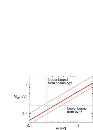
Figure 1: Comparison of the prediction of eq. (17) (thick line) with the general range for $M_{ee}$ allowed with 3 neutrinos (thin lines). The upper bound on $m$ is from Ref. [17]. The lower bound on $M_{ee}$ is the 1 $\sigma$ range in Ref. [54] divided by 2 in order to account for the uncertainty in nuclear matrix elements for the $0\nu 2\beta$ transition ${}^{76}{\rm Ge}\to{}^{76}{\rm Se}\ e^{-}\ e^{-}$.

Assuming degenerate neutrinos, we obtain the most interesting scenario. In fact, when we fix the Majorana phases $\rho$ and $\sigma$, prescribing $|M_{ee}|=|M_{e\mu}|$ and $|M_{\mu\tau}|=|M_{\mu\mu}|$, we immediately realize that it is possible to arrange

$$|M_{\alpha\beta}|=m/\sqrt{3},\ \ \mbox{ where }\alpha,\beta=e,\mu,\tau$$ (17)

setting again $\theta_{13}=0$ and $\theta_{23}=45^{\circ}$, and omitting the small $\Delta M^{2}_{ij}/m^{2}$ terms.

This implies that the limit obtained in cosmology, $m<0.23$ eV at 95 % CL can be translated in a limit on the mass seen in double beta decay:

$$|M_{ee}|<0.13\ \mbox{eV}$$ (18)

This is smaller than the value suggested by the new analysis of the Heidelberg-Moscow data [54] $0.44_{-0.20}^{+0.14}$ eV (at 3 $\sigma$ level), even if one takes $1\sigma$ lower experimental value and assumes that the nuclear matrix elements have been underestimated (see figure 1). Such a small value $m_{\nu_{e}}\approx m\approx 0.23$ eV, being interesting for the forthcoming KATRIN experiment, does not not guarantee a 3 $\sigma$ discovery with the present facility. From eq. (17) one obtains the value of the mass $M_{ee}=0.19$ eV

$$m_{\rm cosm}=3m=1.0\mbox{ eV},$$ (19)

where we used $M_{ee}=0.19$ eV, which is 1 $\sigma$ lower than the value that explains the Heidelberg-Moscow results, reduced by 50 %. This implies that, in deriving cosmological bound the errors were underestimated or the assumptions do not hold. A value $m_{\nu_{e}}\approx m\approx 0.33$ eV should permit a 3 $\sigma$ discovery in KATRIN.

Note that when we assume that the violation of flavor blindness is minimal, the theoretical framework becomes more restrictive and the predictions for the neutrinoless double beta decay process become more precise. This can be understood well from figure 1, since for instance one can reconcile the cosmological bound and Heidelberg-Moscow findings in the 3 neutrino context if $M_{ee}\sim m\sim 0.2$ eV. Of course, under this assumption one has the non-minimal deviations from the flavor blindness.

The case of eq. (17) has been considered for the first time by Frigerio and Smirnov in a phenomenological analysis of all possible neutrino mass matrices: see ref. ([20]), second paper. Our approach permits a step forward, since this is not one case among many other, but the only possible case once that we require that the deviations from flavor blindness are minimal.

3 Renormalization group effects

As we have seen in the previous section, the scales where we want gravity to generate the mass matrix are typical GUT scales or a little lower. Hence one has to consider the effect of renormalization group (RG) evolution from this scale to the electroweak scale on the mass matrix. In both the standard model and its minimal supersymmetric extension, the RG effects are negligible as far as the structure of the mass matrix is concerned. However oscillation observables can be significantly altered, especially for the degenerate mass spectrum. For the parameter space of interest at present to oscillation phenomenology, modulo fine tuning, the effects of RG are not very large [5, 51, 52, 53] except for very large values of the common neutrino mass (that as recalled above are not favored by the data) and of the parameter $\tan\!\beta$ (but only for supersymmetric models).

4 Summary and discussion

We have considered dimension-5 gravity induced operators, suppressed by a low scale of gravity $M_{X}<M_{\rm Pl}$, as the source of the neutrino mass matrix. After spontaneous electroweak symmetry breaking with $\langle\varphi^{0}\rangle=v$, the operator in eq.(2) produces the neutrino mass matrix in flavor basis $M_{\alpha\beta}=\lambda_{\alpha\beta}\;v^{2}/M_{X}$. We assume an approximate flavor blindness when all $\lambda_{\alpha\beta}\sim{\cal O}(1)$. The exact values of $\lambda_{\alpha\beta}$ is a prerogative of the detailed theory of quantum gravity and the wormhole theory.

We have demonstrated that for the degenerate and the inverse hierarchical neutrino mass spectrum there are sets of ${\cal O}(1)$ coefficients when the neutrino masses and mixings satisfy all the observational data. The mass scale for this case is $M_{X}\sim 10^{13}-10^{15}$ GeV, i.e., close to a typical GUT scale. The discussed mechanism is not valid for the hierarchical neutrino mass spectrum.

In the extreme case of unbroken flavor blindness, $\lambda_{\alpha\beta}=1$, the gravity-induced neutrino mass matrix can explain at best the solar-neutrino data and an additional mechanism is needed to provide the atmospheric neutrino mass squared difference.

The gravity-induced textures have interesting predictions for the mass $M_{ee}$ probed in neutrinoless double beta decay. For the inverted hierarchical neutrino mass spectrum the predicted mass parameter $M_{ee}$ is large, 15 - 50 meV. For degenerate spectra, $M_{ee}$ can saturate the bound from cosmology of 0.23 eV or possibly approach the bound of $\sim 1$ eV coming from the studies of tritium endpoint spectra. In both cases it can explain the result obtained from the recent analysis of the Heidelberg-Moscow experiment, although the range of compatibility between this result and cosmology is restricted.

The conclusions of previous paragraph are more generic than that related to gravity-induced neutrino mass model. The specific feature of this model is approximate flavor blindness which favors degenerate mass spectrum of neutrinos. Another consequence of this model is the further narrowing of the compatibility of cosmological bounds and the Heidelberg-Moscow results. As discussed in Sect. 2.3, this is due to the fact that the Majorana phases are fixed by the condition of flavor-blindness: see eq. (17) and fig. 1. Approximate flavor blindness is a natural prediction of the gravity-induced neutrino mass model, but not the exclusive signature of this model. This model can be probed only by combination of the numerical value of fundamental gravity scale, found from other data, and approximate flavor blindness. At present stage of development, we can only argue that this model is a viable possibility.

References

- [1] P.Minkowski, Phys. Lett. B 67, (1977) 421, M.Gell-Mann, P.Ramond and R.Slansky, in Supergravity, ed. P. van Niuwenhuizen and D.Z. Freedman (North Holland 1979), T.Yanagida, in Proc. of Workshop on Unified Theory and baryon number in the Universe, ed. O.Sawada and A.Sugamoto KEK, 1979, R. N. Mohapatra and G. Senjanovic, Phys. Rev. Lett. 44 (1980) 912.
- [2] R. Barbieri, J.R. Ellis and M.K. Gaillard, Phys. Lett. B 90, (1980) 249.
- [3] E.K. Akhmedov, Z.G. Berezhiani and G. Senjanović, Phys. Rev. Lett. 69, (1992) 3013. E.K. Akhmedov, Z.G. Berezhiani and G. Senjanović and Z. Tao, Phys. Rev. D 47, (1993) 3245.
- [4] A. de Gouvea and J.W.F. Valle, Phys. Lett. B 501, (2001) 115.
- [5] F. Vissani, M. Narayan and V. Berezinsky, Phys. Lett. B 571, (2003) 209.
- [6] V.Berezinsky, M.Narayan, F.Vissani, Nucl. Phys. B 658 (2003) 254.
-
[7]
S. W. Hawking,
Phys. Lett. A 60 (1977) 81,
S. W. Hawking, D. N. Page, C. N. Pope, Phys. Lett. 86 (1979) 175,
S. W. Hawking, D. N. Page, C. N. Pope, Nucl. Phys. B 170 (1980) 283. - [8] N. Arkani-Hamed, S. Dimopoulos, G. Dvali, Phys. Lett. B 429 (1998) 263, N. Arkani-Hamed, S. Dimopoulos, G. Dvali, Phys. Rev. D 59 (1999) 086004.
- [9] Z. Berezhiani and G. Dvali, Phys. Lett. B 450 (1999) 24.
- [10] P. Horava and E. Witten, Nucl. Phys. B 460 (1996) 506 and 475 (1996) 94.
- [11] C. Aulakh et al., Phys. Lett. B 588 (2004) 196
- [12] F. Feruglio, A. Strumia and F. Vissani, Nucl. Phys. B 637, (2002) 345 and ibid 659, (2003) 359 (addendum).
- [13] P. Creminelli, G. Signorelli and A. Strumia, JHEP 0105, (2001) 052 and hep-ph/0102234. G.L. Fogli, E.Lisi, A. Marrone, D. Montanino, A. Palazzo and A.M. Rotunno, Phys. Rev. D 67, (2003) 073002. A. Bandyopadhyay, S. Choubey, R. Gandhi, S. Goswami and D. P. Roy, Phys. Lett. B 559, (2003) 121.
- [14] P. C. de Holanda and A. Yu. Smirnov, JCAP, 0302:001 (2003). J. N. Bahcall and C. Pena-Garay, hep-ph/0305159.
- [15] J. Bonn et al., Nucl. Phys. Proc. Suppl, 91 (2001) 273. V.M. Lobashev et al., Nucl. Phys. Proc. Suppl, 91 (2001) 280.
- [16] Heidelberg-Moscow Collaboration, H.V. Klapdor-Kleingrothaus et al., Eur. Phys. J. A 12 (2001) 147.
- [17] D.N. Spergel et al., astro-ph/0302209. Other relevant data and analyses are in Ø. Elgaroy et al., Phys. Rev. Lett 89, (2002) 061301 and A. Lewis and S. Bridle, Phys. Rev. D 66, (2002) 103511.
- [18] Ø. Elgaroy and O. Lahav, JCAP 04, (2003) 004. S.L. Bridle, O. Lahav, J.P. Ostriker and P.J. Steinhardt, Science 299, (2003) 153.
- [19] G. Altarelli and F. Feruglio, Phys. Rept 320, (1999) 295 and ibid Phys. Lett. B 439, (1998) 112.
- [20] M. Frigerio and A. Yu. Smirnov, Nucl. Phys. B 640, (2002) 233 and ibid Phys. Rev. D 67, (2003) 013007.
- [21] A. Ioannisian and J. W. F Valle, Phys. Lett. B 332, (1994) 93.
- [22] H. Fritzsch and Z. Z. Xing, Phys. Lett. B 372, (1996) 265 and ibid 440, (1998) 313 and ibid Prog. Part. Nucl. Phys, 45, (2000) 1.
- [23] R. N. Mohapatra and S. Nussinov, Phys. Lett. B 441, (1998) 229 and ibid Phys. Rev. D 60, (1999) 013002.
- [24] M. Fukugita, M. Tanimoto and T. Yanagida, Phys. Rev. D 57, (1998) 4429 and ibid 59, (1999) 113016.
- [25] Z. Berezhiani and A. Rossi, JHEP 9903 (1999) 002 and Nucl. Phys. B 594 (2001) 113
- [26] M. Tanimoto, T. Watari and T. Yanagida, Phys. Lett. B 461, (1999) 345.
- [27] S. K. Kang and C. S. King, Phys. Rev. D 59, (1999) 091302.
- [28] C. Wetterich, Phys. Lett. B 451, (1999) 397.
- [29] M. Tanimoto, Phys. Lett. B 483, (2000) 417.
- [30] G. C. Branco, M. N. Rebelo and J. I. Silva-Marcos, Phys. Rev. D 62, (2000) 073004.
- [31] G. Perez, JHEP 0012, (2000) 027.
- [32] E. K. Akhmedov, G. C. Branco, F. R. Joaquim and J. I. Silva-Marcos, Phys. Lett. B 498, (2001) 237.
- [33] F. Vissani, Phys. Lett. B 508, (2001) 79.
- [34] P. H. Frampton, S. L. Glashow and D. Marfatia, Phys. Lett. B 536, (2002) 79.
- [35] M. Jezabek, Acta. Phys. Polon. B 33, (2002) 1885.
- [36] S. T. Petcov, Phys. Lett. B 110, (1982) 245; N. Irges, S. Lavignac and P. Ramond, Phys. Rev. D 58 (1998) 035003; J. Sato and T. Yanagida, Phys. Lett. B 430, 127 (1998); R. Barbieri et al, JHEP, 9812, (1998) 01.
- [37] P. Binetruy, S. Lavignac, S. T. Petcov and P. Ramond, Nucl. Phys. B 496 (1997) 3
- [38] G. C. Branco and J. I. Silva-Marcos, Phys. Lett. B 526, (2002) 104.
- [39] E. Ma and G. Rajasekaran, Phys. Rev. D 64, (2001) 113012 and ibid 68, (2003) 071302. K. S. Babu, E. Ma and J. W. F. Valle, Phys. Lett. B 552, (2003) 207.
- [40] J. Kubo et al, Prog. Theor. Phys. 109, (2003) 795.
- [41] W. Grimus and L. Lavoura, Phys. Lett. B 572, (2003) 189.
- [42] P. F. Harrison and W. G. Scott, Phys. Lett. B 557, (2003) 76.
- [43] L. J. Hall, H. Murayama and N. Weiner, Phys. Rev. Lett 84, (2000) 2572. N. Haba and H. Murayama, Phys. Rev. D 63, (2001) 053010. A. De Gouvea and H. Murayama, Phys. Lett. B 573, (2003) 94. J. R. Espinosa, hep-ph/0306019.
- [44] M. Hirsh and S. F. King, Phys. Lett. B 516, (2001) 103. G. Altarelli, F. Feruglio and I. Massina, JHEP 0301, (2003) 035.
- [45] A. Yu. Smirnov, hep-ph/0311259.
- [46] S. Weinberg, Phys. Rev. Lett 43, (1979) 1566.
- [47] S. Coleman, Nucl. Phys. B 307 (1988) 867.
-
[48]
S. B. Giddings and A. Strominger, Nucl. Phys. B 307 (1988) 854.
G.V. Lavrelashvilli, V. A. Rubakov and P. G. Tinyakov, Nucl. Phys. B 299 (1988) 757. - [49] M. Apollonio et al, CHOOZ Collaboration, Phys. Lett. B 466, (1999) 415.
- [50] See e.g., [7, 2, 3] and the discussion in Sect.2.1.1 of V. Berezinsky, M. Narayan and F. Vissani, Nucl. Phys. B 658 (2003) 254.
- [51] P. H. Chankowski and S. Pokorski, Int. J. Mod. Phys A17 (2002) 575.
- [52] S. Antusch, J. Kersten, M. Lindner and M. Ratz, Nucl. Phys. B 674, (2003) 401.
- [53] G. Bhattacharyya, A. Sil and A. Raychaudhuri, Phys. Rev. D 67, (2003) 073004.
- [54] H.V.Klapdor-Kleingrothaus, I.V.Krivosheina, A. Dietz, O. Chkvorets, Phys.Lett. B586 (2004) 198 and Nucl. Instrum. Meth. A 522 (2004) 371.