TAUP

2757/2004

Towards a New Global QCD Analysis: Solution to the Non-Linear Equation at Arbitrary Impact Parameter

E. Gotsman ${\!}^{\mbox{\scriptsize 1)}}$, M. Kozlov ${\!}^{\mbox{\scriptsize 2)}}$, E. Levin ${\!}^{\mbox{\scriptsize 3)}}$, U. Maor ${\!}^{\mbox{\scriptsize 4)}}$ and E. Naftali ${\!}^{\mbox{\scriptsize 5)}}$

School of Physics and Astronomy
Raymond and Beverly Sackler Faculty of Exact Science
Tel Aviv University, Tel Aviv, 69978, ISRAEL

Abstract: A numerical solution is presented for the non-linear evolution equation that governs the dynamics of high parton density QCD. It is shown that the solution falls off as $e^{-b/R}$ at large values of the impact parameter $b$. The power-like tail of the amplitude appears in impact parameter distributions only after the inclusion of dipoles of size larger than the target, a configuration for which the non-linear equation is not valid. The value, energy and impact parameter of the saturation scale $Q_{s}(y=\ln(1/x),b)$) are calculated both for fixed and running QCD coupling cases. It is shown that the solution exhibits geometrical scaling behaviour. The radius of interaction increases as the rapidity in accordance with the Froissart theorem. The solution we obtain differs from previous attempts, where an anzatz for $b$ behaviour was made. The solutions for running and fixed $\alpha_{\rm s}$ differ. For running $\alpha_{\rm s}$ we obtain a larger radius of interaction ( approximately twice as large), a steeper rapidity dependence, and a larger value of the saturation scale.

1 Introduction

The main goal of this paper is to find a numerical solution (including its impact parameter dependence) of the non-linear evolution equation [1], that governs the dynamics of the dipole scattering amplitude in the saturation region [2, 3, 4].

Although, there are several schemes for finding a numerical solution [5, 6, 7, 8], we still lack a reliable method that will allow us to study the properties of the solution of the non-linear evolution equation. For example, there is the difficulty of understanding the large impact parameter ($b\equiv|\vec{b}|$) behavior of the solution. Our notation is such that the symbol “$\rightarrow$” represents a two dimensional vector, in the transverse plane.

The large $b$ behavior is strongly affected by the non-perturbative contributions [9], since in pQCD the amplitude falls off as a power of $b$. A decrease of this type leads to a power-like growth of the interaction radius, which violates the Froissart bound [10]. This difficulty can be overcome by introducing non-perturbative corrections for large $b\,\,(\,\,>\,\,1/m_{\pi})$, where $m_{\pi}$ is the mass of the lightest hadron ($\pi$-meson). Two suggestions of how to include such non-perturbative corrections have been made : (i) to change the kernel of linear and non-linear equations [9]; and (ii) to accumulate all non-perturbative corrections in the initial conditions of the equation [11, 12, 13]. The first attempt to solve the full non-linear equation including the impact parameter behavior, was made in Ref. [14]. The solution of Ref. [14], shows that to obtain the correct behavior at large values of $b$, one has to alter the kernel of the equation.

We examine this solution and show that the entire power-like decrease obtained in Ref. [14], originates in the kinematic region where the non-linear equation is not trustworthy.

In our search for the solution we are guided by: (i) the known analytic expressions for the simplified cases [15, 16, 13], and (ii) practical experience gained in previous attempts:

1. The non-linear evolution equation can be viewed as the sum of the semi-enhanced, ‘fan’ diagrams (see Fig. 1a for such a diagram). However, we should restrict ourselves to summing such diagrams only for the scattering amplitude of a dipole of transverse size ($|\vec{r}|$), which is much smaller than the size of the target [2, 3] ($|\vec{r}|\ll R$, where $R$ is the target transverse size). If the target is smaller than the projectile, we need to sum diagrams of the type shown in Fig. 1b. Although, the kernel of the non-linear equation does not depend explicitly on the size of the target, this quantity appears in the solution by way of the region of validity of the equation.

2. In the saturation region ($\vec{r}\leq\,2/Q_{s}$, where $Q_{s}$ is the saturation scale) the solution displays geometrical scaling [15, 13, 21, 4], namely, the scattering amplitude $\cal{A}$ is a function of only one variable

   $$N\left(\vec{r},b;x\right)\,\,\equiv\,\,\mbox{Im}A\left(\vec{r},\vec{b};x\right)\,\,\,=\,\,\,N\left(r^{2}\,\,Q_{s}(x;b)\right).$$ (1)

   We therefore expect that the entire $b$ dependence can be absorbed into the saturation scale $Q_{s}(x;b)$.

3. We examine the behaviour of the scattering amplitude $N\left(\vec{r},\vec{b};x\right)$, both for the case of the running QCD coupling constant, and for fixed $\alpha_{s}$.

4. In the saturation region $N\left(\vec{r},\vec{b};x\right)<1$, consequently the non-linear equation has a solution that satisfies $s$-channel unitarity. On the other hand, the behavior of the total cross section:

   $$\sigma^{\mathrm{dipole}}(\vec{r},x)\,\,=\,\,2\,\,\int\,d^{2}\,b\,\,N\left(\vec{r},b_{t};x\right)\,$$ (2)

   depends critically on the large $b$ dependence of the amplitude, and has to be studied separately.

5. The semiclassical solution [13] to the non-linear evolution equation, indicates that the behaviour at large $b$ stems from the initial conditions.

Our strategy is to assume that the size of the interacting dipole is smaller than that of the target. In the next section we describe the method of solution which we develop based on this strategy. In Section 3 we present our results. In particular, we check whether the geometrical scaling behavior in the form of Eq. (1) occurs in our solution. In the Conclusions, we discuss the main results and the possibility of using them for phenomenology.

2 Method of the Solution

The nonlinear evolution equation[1] characterizes the low $x$ behavior of the parton densities, while taking into account hdQCD effects, so that unitarity constraints are inherently obeyed.

We denote by $N$ the imaginary part of the interaction amplitude of a target with a parent dipole, of transverse size $\vec{r}$ and two dipoles, of transverse sizes $\vec{r}_{1}$ and $\vec{r}_{2}\,$ ($\vec{r}=\vec{r}_{1}+\vec{r}_{2}$), produced by $\vec{r}$.

The probability for the decay $\vec{r}\rightarrow\vec{r}_{1},\vec{r}_{2}$ is given by the square of the wave function of the parent dipole, which, in a simplified form, can be written as $r^{2}/r^{2}_{1}r^{2}_{2}$. Each of the produced dipoles can interact with the target independently, with respective amplitudes $N(y,\vec{r}_{2};\vec{b}-\mbox{\small$\frac{1}{2}$}\vec{r}_{1})$ and $N(y,\vec{r}_{1};\vec{b}-\mbox{\small$\frac{1}{2}$}\vec{r}_{2})$, where $y$ denotes the rapidity variable ($y=-\ln x$) and $\vec{b}$ the impact parameter in the transverse plane. Adding these contributions, clearly overestimates the dipole-nucleon interaction, since there is the probability that during the interaction, one dipole can be in the shadow of the other. This correction is given by an additional negative quadratic term $-N(y,\vec{r}_{2};\vec{b}-\mbox{\small$\frac{1}{2}$}\vec{r}_{1})N(y,\vec{r}_{1};\vec{b}-\mbox{\small$\frac{1}{2}$}\vec{r}_{2})$.

(a)                                                    (b)

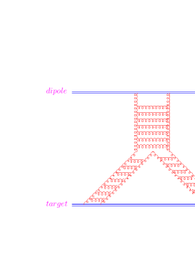
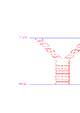
Figure 1: Multiple emissions of small $x$ gluons: (a) from the target, and (b) from the dipole.

In the procedure leading to the construction of the non-linear evolution equation, only fan diagrams of the type shown in Fig. 1a were taken into account, while fan diagrams having multiple emissions from the parent dipole (Fig. 1b) were omitted [1]. In other words, the equation does not include contributions for $|\vec{r}_{1}|,|\vec{r}_{2}|>R$, where $R$ is the transverse size of the target. The solutions, that have been presented previously in Refs. [5, 6, 7, 14], included contributions from both large and small size dipoles.

Our approach is initially to exclude contributions from large dipoles, and then to estimate the accuracy of this proceedure by employing a second iteration. The price we pay for this approach is, that our calculations are only valid for short distances, compared to the size of the target. Nevertheless, as we shall demonstrate later, contributions coming from large dipoles, which we consider as a correction, are relatively small.

Hence, we can write the evolution equation in a differential form as:

$$N_{y}(y,{\vec{r}};\vec{b})\equiv{\partial N(y,{\vec{r}};\vec{b})\over\partial y}=\frac{2C_{F}\alpha_{\rm s}}{\pi^{2}}\int d^{2}r_{2}\frac{r^{2}}{r^{2}_{1}r^{2}_{2}}\,\theta(R-|\vec{r}_{1}|)\,\theta(R-|\vec{r}_{2}|)\,$$ (3)

$$\left[2N(y,\vec{r}_{1};\vec{b}-\mbox{\small$\frac{1}{2}$}\vec{r}_{2})-N(y,\vec{r}_{1};\vec{b}-\mbox{\small$\frac{1}{2}$}\vec{r}_{2})\,N(y,\vec{r}_{2};\vec{b}-\mbox{\small$\frac{1}{2}$}\vec{r}_{1})-N(y,\vec{r};\vec{b})\right]\,.$$

The $\vec{r}_{2}$ integration in (3) is regulated by introducing an ultraviolet cutoff, which does not affect the physical quantities.

Strictly speaking, the evolution equation is defined for fixed strong coupling, $\alpha_{\rm s}$. Since for running $\alpha_{\rm s}$ it is difficult to define the running scale in terms of the variables of integration, $\vec{r}_{1}$ and $\vec{r}_{2}$, of the r.h.s of Eq. (3). In the semiclassical approach, however, one sets $\alpha_{\rm s}=\alpha_{\rm s}(4/r^{2})$, i.e. one uses the size of the parent dipole, as the running scale of the coupling. In the following, we shall attempt to compare the results obtained with fixed coupling to those obtained with running coupling in the semiclassical approach. Another approach would be to calculate the solution using $\alpha_{\rm s}=\alpha_{\rm s}((2\vec{r}_{1}\vec{r}_{2}/(\vec{r}_{1}+\vec{r}_{2}))^{2})$, but such a calculation is beyond the scope of the present work.

The strong coupling constant $\alpha_{s}$ is chosen to run according to the prescription

$$\alpha_{s}(r)\;=\;\frac{4\pi}{\beta_{0}\;\ln(4/(\Lambda^{2}_{QCD}r^{2}))}$$

where $\Lambda_{QCD}$ = 0.2 GeV and $\beta_{0}$ = (33 - 2$n_{f}$)/3. For the case of fixed coupling constant we take $\alpha_{s}$ = 0.2.

To obtain a solution to (3) at arbitrary $b$, one needs to specify the initial conditions of $N$ at $y=y_{0}$, the rapidity from where we commence the evolution. The initial condition is a function of both $\vec{r}$ and $\vec{b}$ at $y=y_{0}$, while our goal is to obtain a solution, which is a function of $\vec{r}$ and $\vec{b}$ for all $y\geq y_{0}$. We are aware that during the evolution process, as $y$ increases, the role played by the initial input decreases, and the evolution becomes the dominant factor influencing the dynamics per se.

The experience we have in solving Eq. (3) (both with fixed and running $\alpha_{\rm s}$) stems mostly from the solution of the equation, where shifts in $\vec{b}$ on the r.h.s. of the equation, were neglected. For such a simplified equation, the impact parameter is treated as a fixed parameter in the procedure. For a solution of the type found in [6], once a trial solution was found at sufficiently large $y$, the curve approximating the solution was rescaled at fixed $b$ assuming geometrical scaling [see Eq. (1)], so as to reproduce the initial conditions at $y=y_{0}$. The reconstructed initial conditions were then used as input for the evolution, so that, the final solution almost completely decoupled from the initial input. It was demonstrated in [6] that the initial conditions obtained in this fashion, at very large distances, provide a smooth extrapolation of the Glauber formula to unity.

In this paper we adopt the basic principle of this procedure, and use the rescaled solution of [6] to construct the initial conditions. At first sight, it appears sufficient to follow [6] by adopting the fixed $b$ solution as input, and assuming the following ansatz for the $b$-dependence:

$$N(y_{0},\vec{r};\vec{b})=1\,-\,e^{-\kappa(y_{0},\vec{r})\,S(\vec{b})/S(0)}\,,$$ (4)

where $S(\vec{b})$ is the profile function (e.g., a Gaussian or a dipole-like profile) and

$$\kappa(y_{0},\vec{r})=-\ln\left(1\,-\,N(y_{0},\vec{r};b=0)\right).$$ (5)

However, in the Born approximation, at a finite mass of the gluon field, the scattering amplitude for large size parent dipoles, decreases already at $b=0$. To facilitate such behavior, we modify (4) as follows:

$$N(y_{0},\vec{r};\vec{b})=1\,-\,e^{-\kappa(y_{0},\vec{r})\,S(\sqrt{b^{2}+r^{2}})/S(0)}\,.$$ (6)

Figs. 2a-b show a comparison for the initial conditions of Eqs. (4) and (6). The replacement $b^{2}\longrightarrow b^{2}+r^{2}$, suppresses the initial conditions at large $r$, thereby smoothing the $\theta$ functions of (3).

Figure 2: The solution of the non-linear evolution equation for different initial conditions: (a) using Eq. (4) with a Gaussian profile function; (b) using Eq. (6) with the same profile.

The most troublesome contribution in Eq. (3) comes from the region of $r_{1}$ and/or $r_{2}$ of the order of $2b$. Indeed, in this region at large values of $b$, the r.h.s. of the master equation can be rewritten in the form

$$\Delta N\,\,=\,\,\frac{r^{2}}{b^{4}}\,\,\int d^{2}\Delta b\,\left(\,2\,N(y,b,\Delta b)\,-\,N^{2}(y,b,\Delta b)\,-\,N(y,r,b)\right)$$ (7)

One can see that $\Delta N\propto\,1/b^{4}\,$ at large $b$. This contribution has been discussed in Ref. [9, 14]. We claim that this contribution originates from the interaction of the dipoles of size much larger than the size of the target, and that it cannot be evaluated using Eq. (3).

Apart from rapidity, the function $N$ depends on the dipole’s degrees of freedom, which are the transverse separation of the parent dipole, $\vec{r}$, and the transverse impact parameter, $\vec{b}$. We therefore, define the following variables, through which we express the dipole-nucleon amplitude: $r\equiv|\vec{r}|$, $b\equiv|\vec{b}|$, and $\hat{r}_{||}\equiv\vec{b}\cdot\vec{r}/(br)$. In the following, we shall concentrate on the integrated quantity $N(y,r;b)\equiv\int d\hat{r}_{||}N(y,r;b;\hat{r}_{||})$.

Once the initial conditions were established, we applied the following numerical procedure, which has four stages:

1. First iteration: we denote by $y_{i}$ a particular rapidity, at which the solution and its derivative are known for all values of $r\,,b$ and $\hat{r}_{||}$. The solution at $y_{i+1}\equiv y_{i}+h(y)$ was constructed as a matrix, in which the matrix elements correspond to (fixed $y$) solutions at different $r$ and $b$, integrated over $\hat{r}_{||}$:

   $$N^{(1)}(r,y_{i+1};b)=N^{(1)}(r,y_{i};b)+h(y_{i})\int d\hat{r}_{||}\left.N_{y}^{(1)}(y,r;b;\hat{r}_{||})\right|_{y=y_{i}}\,,$$ (8)

   where $N_{y}^{(1)}$ is given by the R.H.S of (3), and $h(y_{i})$ is a variable step size in the rapidity space. The first iteration included successive constructions of such matrices over a range of about 10 units of rapidity, starting from $y_{0}\approx 4.6$. The value of $h(y_{i})$ was chosen dynamically to ensure that the maximal error over the $i$th matrix is small (we set our accuracy condition to $10^{-3}$). We used the Euler two-step procedure to select $h(y)$, we found that the optimal step size may vary from $h\approx 0.01$ for small rapidities to $h\approx 0.2$ for large rapidities. The CPU time for the entire iteration was about $20$ hours for $30\times 30$ matrices.

   Our main claim is that the first iteration as described above, provides a reliable solution to the master equation.

2. First Correction: in order to check the accuracy of the first iteration, and to estimate the importance of long distance contributions, we substituted $N^{(1)}$ back into the non-linear evolution equation, and recalculated $N_{y}$ in the kinematical region which was omitted from (3), namely for $|\vec{r}_{1}|,\,|\vec{r}_{2}|>R$. In other words, we calculated the contribution given by Eq. (7). We consider the result of this calculation an estimate of the correction to $N_{y}^{(1)}$, and denote it by ${\Delta N_{y}^{(1)}}$.

3. Second iteration: to estimate the influence of the neglected terms on the behavior of the solution in the saturation region, we calculated the second iteration. Namely, we used the calculated ${\Delta N_{y}^{(1)}}$ (see Eq. (7)) as a second iteration, by adding the correction to the r.h.s of (8):

   $$N^{(2)}(y_{i+1},r;b)=N^{(2)}(y_{i},r;b)+h(y_{i})\left({\Delta N_{y}^{(1)}}(y_{i},r;b)+\int d\hat{r}_{||}\left.N_{y}^{(2)}(y,r;b;\hat{r}_{||})\right|_{y=y_{i}}\right)\,.$$ (9)

4. Second correction: finally, we calculated ${\Delta N_{y}^{(2)}}$, the correction to the second iteration, by performing the integration over long distances as before.

This procedure gives us full control both on the accuracy of the solution, and on the region of its applicability.

Figure 3: The corrections to the first and the second iterations for $b=0$ and $b=2\,\mbox{GeV}^{-1}$ .

The corrections of the first and second iterations are shown in Fig. 3, for $b=0$ and $b=2\,\mbox{GeV}^{-1}$, as a function of the ratio $r/R$. For not too large rapidities ($y<10$), the corrections are of order 10% , even when the transverse size of the dipole $r$, is comparable to the transverse size of the target, $R$. For larger values of $y$, the corrections are small only for short distances. The second iteration is important at large rapidities where $|\Delta N_{y}^{(2)}|<|{\Delta N_{y}^{(1)}}|$. On comparing $\Delta N$ for both iterations, we see that we can only trust our solution for $r/R\,<\,0.4$ at large values of rapidity ($y>10$), while for small values of $y$ the accuracy of our solution is satisfactory, even for values of $r/R\approx 1.5$. This observation is most encouraging as we would like to use the solution to describe experimental data, which are mostly concentrated at $y<10$.

3 Evolution Results

3.1 $r$, $y$ and $b$ dependence:

Fig. 4 shows the evolution process from $y=4.6$ to $y=14$ at $b=0,\,1,\,3\,{\,\mbox{GeV}^{-1}}$ as a function of $r/R$, and Fig. 5 shows the energy dependence of the amplitude at $b=0$, for different values of $r/R$. We have chosen a target size of $R^{2}=3.1{\,\mbox{GeV}^{-2}}$ so as to compare with [6], where the fixed $b$ solution was successfully fitted to the HERA experimental $F_{2}$ data, using $R^{2}$ as a parameter. In the next section, we discuss in more detail the differences and similarities between the present work and the solutions of [6, 14].

Referring to Fig. 4, we see that at the beginning of the evolution process, the amplitude increases mildly with the dipole size, and does not exhibit saturation in the region of $r<R$. As $y$ increases, the rise of $N$ becomes steeper. This rise is tamed when the impact parameter becomes large.

Figure 4: The evolution of $N$ as a function of $r/R$, for fixed $b$.

In our approach, only the kinematical region $r/R\;\raisebox{-1.72218pt}{\hbox to0.0pt{$\sim$\hss}}\raisebox{1.72218pt}{$<$}\;1$ can be explored accurately , although, there are some other kinematical regions where the corrections ${\Delta N_{y}^{(1)}}$ and ${\Delta N_{y}^{(2)}}$ are relatively small. At long distances there remain considerable theoretical uncertainties.

Figure 5: The energy dependence of $N$ at $b=0$, for different values of $r/R$.

Fig. 7 shows the $b$-dependence of our solution for $r/R=1$. It was argued in [14], that for small rapidities the evolution process starts to generate a power behavior of $b^{-3.6}$, which becomes even milder at higher rapidities. The change in behavior is due to large dipole configurations, which has been discussed above. To illustrate the behavior of $N$ as a function of the impact parameter, we have parameterized our solution as:

$$N(y,r,b)=\frac{f(r,y)S(b)}{1+g(r,y)S(b)}\,,$$ (10)

where $S(b)=(R^{2}+b^{2})^{-2}$ and $f$ and $g$ are fitted functions. Eq. (10) is presented in Fig. 6 as a dashed line. In our approach, since we exclude large dipoles from the evolution, the amplitude at large $y$ deceases with $b$ faster than $b^{-4}$.

Figure 6: The impact parameter dependence of $N$ for $r/R$=1. The dashed line corresponds to the $b^{-4}$ parameterization of Eq. (10).

As was pointed out in Ref.[9] the power-like decrease leads to power-like growth of the average $b^{2}$ as a function of energy. However, Fig. 7 shows that at large values of the dipole size there is only a slow increase, (if at all). Indeed, the simple formula $\langle b^{2}\rangle=a+b\,y+cy^{2}$ provides a good description of the enegy behaviour of the radius of interaction, for different values of $r$. (see Fig. 7).

Figure 7: Energy behavior of the average $b$ at different values of the dipole size for fixed (solid) and running (dashed) QCD coupling.

We have also used Eq.(10) to parameterize the correction $\Delta N^{(1)}\equiv\int{\Delta N_{y}^{(1)}}dy$. In Fig. 8 we show $\Delta N^{(1)}$ and its $b^{-4}$ parameterization for large $r/R=4$ and large $y=14$, we stress that the power tail originates from the correction to the first iteration.

Figure 8: The impact parameter dependence of $\Delta N$. The dashed line corresponds to the $b^{-4}$ parameterization of Eq. (10), employed for $\Delta N^{(1)}$.

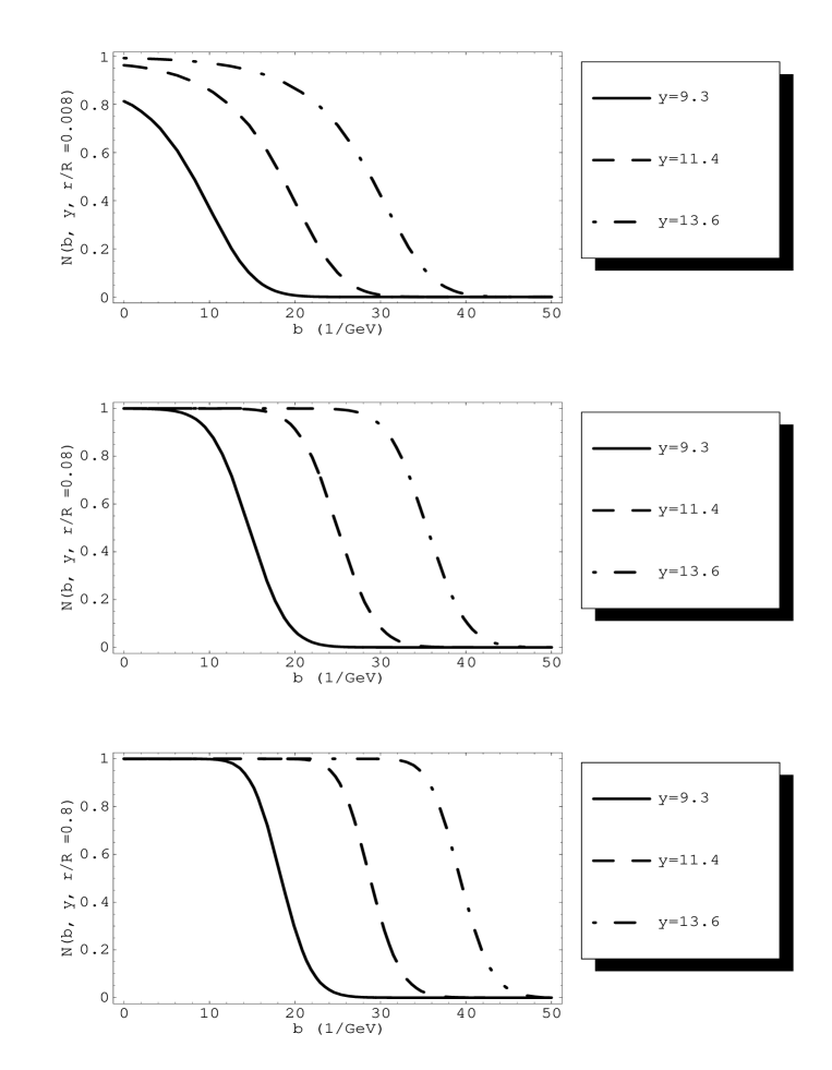
Figure 9: Our solution for the scattering amplitude $N$ as function of the impactparameter $b$, at different energies and at different values of $r$ for running QCD coupling.

Figure 10: Our solution for the scattering amplitude $N$ as function of the impact parameter $b$, at different energies and at different values of $r$ for fixed QCD coupling.

Fixed $\alpha_{\rm s}$		Running $\alpha_{\rm s}$

Figure 11: The large impact parameter behaviour of the scattering amplitude $N$ for fixed and running $\alpha_{\rm s}$.

Fig. 9 and Fig. 10 demontstrate the essential difference between running and fixed QCD coupling cases. One sees that for running QCD coupling the amplitude has a steeper growth with energy, reaching the saturation boundary for smaller $y$ than in the case of fixed $\alpha_{\rm s}$. On the other hand, the behaviour of the tail in the impact parameter distribution looks very similar in both cases (see Fig. 11). It should be stressed that the scattering amplitude falls off exponentially at large $b$ ( $N\,\propto e^{-m\,b}$ with $m$ = 1 to 2 GeV, see Fig. 11 ). Fig. 8 and Fig. 11 show that our solution has no power-like tails in the $b$ distribution, and therefore, supports our hypothesis that the power-like large $b$ decrease, stems from the dipole configuration which cannot be treated within the non-linear Balitsky - Kovchegov equation.

3.2 Saturation scale

We shall now use our solution to the non-linear evolution equation to investigate saturation effects and scaling properties of the dipole-nucleon scattering amplitude. First, we calculated the saturation scale $r_{s}(y,b)$ as being the value of the dipole size, at which the amplitude

$$N(r_{s},y,b)=1\,-\,e^{-1}=0.632$$ (11)

Fig. 12 shows the solution to Eq. (11). We recall, that for the case of fixed QCD coupling in the semiclassical solution (see Ref. [13]) we expect that at large $y$ and $b$

$$Q^{2}_{s}(y,b)\,\,\propto\,\,e^{\lambda y}\,e^{-\frac{b}{R}},$$ (12)

where the estimate for the value of $\lambda$, is $\lambda=4\alpha_{S}$ and $R$ is the radius of the target.

For the running QCD coupling constant, the situation is more interesting (see Ref. [2, 23, 13]): (i) as function of $y$

$$Q^{2}_{s}\,\,\propto\,\,e^{\sqrt{\lambda_{R}\,\,y}}$$ (13)

in the region of $b\,\,<\,\,R\,\lambda_{R}\,y$ ; and (ii) for $b\,\,>\,\,R\,\lambda_{R}\,y$

$$Q_{s}\,\,\propto\,\,e^{-\frac{b}{R}}\,\,;$$ (14)

with $\lambda_{R}\,\,\approx\,\,10$.

To aid in understanding the main features of the energy and impact parameter dependence of the saturation scale, we fitted the result for the saturation momentum using the following parameterizations, which reflect the above semiclassical properties:

$$\mbox{At fixed }b\mbox{:} Q_{s}(y,b)\,\,=\,\,C_{y,1}\,e^{\lambda_{F}\,y}\,\,+C_{y,2}\,e^{\sqrt{\lambda_{R}\,y+a}}$$ (15)

$$\mbox{At fixed }y\mbox{:} Q^{2}_{s}(y,b)/4\,\,=\,\,\frac{C_{b,1}}{C_{b,2}+\,e^{(\frac{(b+C_{b,4})}{C_{b,3}\,R})^{2}}}$$ (16)

Fixed $\alpha_{\rm s}$	Running $\alpha_{\rm s}$

Figure 12: The saturation scale as a solution to Eq. (11) of the amplitude for fixed and running QCD coupling, for different values of $y$ and $b$.

In Fig. 13 we show how these parameterizations describe the calculated saturation momentum for fixed $b$. For running QCD coupling we used the value of $\lambda_{R}$ = 0.26 to 0.30, which is much smaller than the semiclassical prediction: $\lambda_{R}=10$. For fixed QCD coupling, we see an exponential growth with the value of $\lambda_{F}\approx$ 1.4 to 1.6, which is approximately two times larger than the theoretical prediction, $\lambda_{F}=4\alpha_{\rm s}\approx 0.8$.

Both $\lambda_{F}$ and $\lambda_{R}$ turn out to be independent of $b$.

Fixed $\alpha_{\rm s}$	Running $\alpha_{\rm s}$

Figure 13: The energy behavior of the saturation momentum $Q_{s}=2/r_{s}$ for fixed and running QCD coupling. For small $y$ the curve is $\ln Q_{s}=a+\frac{\lambda_{F}}{2}\,\,y$, while for large values of $y$ the curve corresponds to $\ln Q_{s}=a+\frac{1}{2}\,\sqrt{\lambda_{R}+b}$. The results of our calculations are presented as circles whose magnitude reflect the size of possible numerical errors.

Fixed $\alpha_{\rm s}$	Running $\alpha_{\rm s}$

Figure 14: The impact parameter ($b$) behaviour of the saturation momentum $Q_{s}=2/r_{s}$ for fixed and running QCD coupling. The curve correspond to Eq. (15).The results of our calculations are presented as circles whose magnitude reflect the size of possible numerical errors.

Fixed $\alpha_{\rm s}$	Running $\alpha_{\rm s}$

Figure 15: Large impact parameter ($b$) behaviour of the saturation momentum $Q_{s}$ for fixed and running QCD coupling. The curve corresponds to $Q_{s}=C\,\,e^{-m\,b}$ . The results of our calculations are presented as circles whose magnitude reflect the size of possible numerical errors.

Fig. 14 shows the impact parameter behavior of the saturation scale. Both $y$ and $b$ behaviour of the saturation scale are in a qualitative agreement with the expectations mentioned above. The formula given in Eq. (16) describes the main features of the $b$-behavior rather well. For fixed QCD coupling, we see that for a wide range of $y$ we have a Gaussian behavior, while for the case of running QCD coupling the decrease sets in, only in the region of very large $b$. However, the surprising fact is that even at fixed $\alpha_{S}$ for large $y$, the $b$-behavior tends to the same distribution as in the running $\alpha_{S}$ case. This observation requires a qualitative explanation. Note that at large $b$ in both cases, the impact parameter dependence appears to be Gaussian, with a radius of interaction which increases with energy. In our parametrization the radius is equal to $R_{interaction}=C_{3}\,R$ and $C_{3}\,\,\propto\,\,y$.

In Fig. 15 the large $b$ behaviour of the saturation scale is plotted. $Q_{s}$ falls off as $e^{-0.5\,b}$ . One expects such an exponential behaviour from general properties of analyticity and crossing symmetry [10], and this behaviour supports our point of view that the initial conditions determine the large $b$ behaviour of the scattering amplitude.

Fixed $\alpha_{\rm s}$	Running $\alpha_{\rm s}$

Figure 16: The scaling behavior of the amplitude for fixed and running QCD coupling.

3.3 Geometrical scaling

In [2, 4, 21] it was shown that the dipole-nucleon scattering amplitude exhibits scaling, which occurs due to the relationship between the $y$ and $r$ dependences of $N$. This scaling behavior was confirmed in the approximate solution of the non-linear equation [24], without theoretical knowledge of the impact parameter behavior. More specifically, the scaling property implies that, in the kinematical region where saturation occurs, the amplitude is a function of one variable $\tau\equiv rQ_{s}(y,b)$, with $Q_{s}=2r_{s}^{-1}$.

In Fig. 16 our solution is plotted as function of $\tau$. A glance at this figure shows that the solution displays the scaling properties at large values of $y$, as was predicted by theory [21]. On the other hand, Fig. 16 clearly displays that geometrical scaling behavior is more pronounced, for the running QCD coupling constant case.

The improved geometrical scaling which we observe for the running coupling may, at first sight, be confusing, since $\alpha_{s}$ contains a new dimensional parameter $\Lambda_{\mathrm{QCD}}$, which in principle could spoil the scaling. However, in Ref. [13] it has been suggested that the running of the QCD coupling freezes at the saturation scale, thus recovering the broken geometrical scaling property. We interpret our numerical solution, as supporting this hypothesis.

Nevertheless, as the exact definition of the saturation region is a debatable point, we shall also investigate the scaling property of $N$, using the ratio:

$${\cal R}=\frac{\partial N(y,r,b)/\partial y}{\partial\ln N(y,r,b)/\partial r}\,.$$ (17)

If scaling does exist, ${\cal R}$ should equal $\partial\ln Q_{s}(y,b)/\partial y$. Note, that the scaling property of $N$ implies that in the saturation region, ${\cal R}$ should not depend on $r$.

In Fig. 17 we present the ratio ${\cal R}$ as a function $r$, for different values of $y$ and $b$. Although, as stated, our solution is only applicable at small values of $r$, we see that for long distances (for $r/R>0.07$ with $R=\sqrt{3.1}\,{\,\mbox{GeV}^{-1}}$)) ${\cal R}$ is reasonably flat as a function of the dipole size, while for smaller values of $r$ the ratio falls steeply as a function of $r$. Once more, the geometrical scaling behaviour is more striking for the running QCD coupling case. The second interesting observation is that this behaviour is concentrated at small $b$, while at large values of $b$ we see a strong violation of geometrical scaling.

Fixed $\alpha_{\rm s}$	Running $\alpha_{\rm s}$

Figure 17: Scaling ratio ${\cal R}$ as a function of dipole size $r$ for different values of $y$ and $b$.

3.4 Comparison with other solutions

The solution in [6] was the first step at solving the equation for fixed impact parameter. This solution provided an excellent reproduction of the $F_{2}$ HERA data with $\chi^{2}/\mbox{n.d.f.}=1$, using $R^{2}=3.1\,{\,\mbox{GeV}^{2}}$. In Fig. 18 we compare our solution (with the initial conditions of Fig. 2b) and the solution of [6] (with the initial conditions of Fig. 2a). Fig. 18a shows the amplitude as a function of $r/R$. The $r$-dependence of the solutions is substantially different. We see that the $b$-dependence of the equation generates a rapid rise of the amplitude as a function of $r$.

Fig. 18b shows the $b$-dependence of the two solutions. The impact parameter dependence of our present solution is the result of the evolution process (starting from the input of Fig. 2b), whereas the impact parameter dependence of [6] was put by hand, according to the Glauber-Mueller formula $N(b)=1-\exp(-\kappa S(b))$, with $\kappa=-\ln(1-N(b=0))$. The generated $b$-dependence differs from the ansatz of [6]. For low energy (e.g., $y=5.6$) the fixed $b$ solution extends to larger values of the impact parameter, whereas at large energies ($y=9.8$) our present solution lies well above the fixed $b$ solution for values of $b$ about up to $b=10$, where both solutions are small. Only for intermediate energies and distances ($y\approx 7$, $r\approx R/2$), do the two approaches exhibit similar behavior.

In Fig. 18c we show how the two solutions differ in terms of the total cross section, i.e., the area under the curves of Fig. 18b. Only for $y\approx 7$ and small distances do we find similarities between our present solution and the fixed $b$ solution of [6].

Figure 18: Comparison of our solution (solid) and the fixed $b$ solution [6] (dashed). The comparison is for (a) the $r$-dependence of the amplitude at $b=0$; (b) the $b$-dependence of the amplitude at $r=R/2$; and (c) the integrated amplitude, $\int d^{2}bN(y,r,b)$ as a function $r/R$.

Fig. 19 shows a qualitative comparison of our solution and the solution of Ref. [14]. Only a qualitative comparison can be made here, as (i) in [14] there was an explicit $\cos\theta$ dependence, where $\theta$ is the angle between $\vec{r}$ and $\vec{b}$, whereas our solution is an integrated quantity, $N(y,r;b)\equiv\int d\hat{r}_{||}N(y,r;b;\hat{r}_{||})$; and (ii) there is a normalization difference, due to the different scales at which the dimensional variables are defined.

The origin of the last difference is the different initial conditions that were used. In [14] a pure Glauber-Mueller form for the initial conditions was assumed, using a profile $S(b)=10\exp{(-b^{2}/2)}$. Our initial conditions, on the other hand, have a different shape (see Fig. 2b) and are based on parameters which were established for our fits to the HERA data [6].

To enable us to make an illustrative comparison, we have used the following procedure:

1. To minimize the angular sensitivity, we compare the two solutions only at low $r$ or low $b$.

2. We interpreted the input impact parameter dependence of [14] (  i.e. $S(b)\propto\exp(-b^{2}/2)$ ), as $\exp{-b^{2}/R^{2}}$ with $R^{2}=2$. Recalling that we use $R^{2}=3.1{\,\mbox{GeV}^{2}}$ as the size of the target, we have rescaled $b$ according to $b^{2}\longrightarrow 2b/3$, hence matching the dimensional units of [14].

3. The shape of our initial input (see Fig. 2b) is substantially different from the Gaussian of [14]. On the other hand, we wish to compare the solution at $y>y_{0}$, where we assume that $N$ has a weak dependence (if any) on the shape of the initial conditions. Thus, we have chosen to rescale $r$ so that after evolution of, say, two units of rapidity, the two solution will match at small $b$ and fixed $r$. We found that a rescaling of $r\longrightarrow 2r$ is sufficient to produce such matching.

Referring again to Fig. 19 we see that as a function of $b$, our solution decreases more rapidly. In addition, we see that as a function of $r$ and $b=0$, the large normalization difference between the two solutions at $y-y_{0}=2$ diminishes at sufficiently large $y-y_{0}=9$. The $b$-dependence of the saturation scale $Q_{s}$ is similar, but there is a considerably large normalization difference, which may be due to disparities in the definition of the saturation region, and the above mentioned dimensional parameters.

Figure 19: Comparison between our solution (solid) and the solution of [14] (dashed).

4 Summary

In this section we summarize the main features of our numerical solution of the non-linear evolution equation.

• It is shown that the non-linear equation in the region where it’s validity is guaranteed, leads to a solution which falls off as

  $$N(r,b;y)\,\,\,\propto\,\,\,e^{-\frac{b}{R}}\,\,\,\,\,\,\mbox{for large}\,\,\,\,\,\,b\,>\,\,\lambda\,y\,\,;$$ (18)

• We showed that the inclusion of dipoles of size larger than the target ($R$), generate the power-like tail in impact parameter distributions. This means that the power-like behaviour is an artifact of using the non-linear equation, for calculating the scattering amplitude in the kinematic region, where this equation is not valid ( see Refs. [25] for an approach that can describe this region);

• In our approach we modified the kernel of the non-linear equation by introducing $\Theta(R-r_{1})\,\Theta(R-r_{2})$. We concur with the idea of Ref.[9] that to obtain the correct (exponentially decreasing) large impact parameter dependence, it is necessary to change the kernel of the non-linear equation. On the other hand, the non-linear equation was obtained implicitly assuming that the size of the projectile dipole is much smaller than the size of the target. This was a misconception based on the semiclassical approach, and on the exact solution for the simplified double logarithmic kernel for $r\,\ll\,R$, that large dipoles will not appear in the intermediate stage of evolution [11, 12]. We demonstrated that the large $b$ tail which behaves as $1/b^{4}$, stems entirely from the large dipole contribution, even for small $r$. The large $b$ tail gives a very small contribution to the amplitude. One can compare Fig. 10 with the value of $\Delta N$ in Fig. 8, to realize that $\Delta N/N$ is negligible for $b\,>\,25\,\,GeV^{-1}$. Therefore, the statement of Refs. [11, 12] looks reasonable, that the large $b$ tail which is a problem in the pQCD approach, does not contributute to the main physical observables, including the total cross section.

• The value, energy and impact parameter dependence of the saturation momentum are calculated. We find that at large values of rapidity, the value of the saturation momentum no longer depends on the impact parameter $b$. A behaviour of this type was predicted for $Q_{s}$ in the case of running QCD coupling [23], but was not expected for fixed $\alpha_{S}$;

• The geometrical scaling behaviour of the scattering amplitude is discussed, and we show that the scattering amplitude can be displayed as a function of one variable $\tau=r\,Q_{s}(y,b)$. The geometrical scaling behaviour is more striking for the running QCD coupling, than for fixed $\alpha_{s}$. An explanation for such behaviour could be related to the idea [13], that the running QCD coupling is frozen at the saturation scale. In this case the smallness of $\alpha_{S}(Q_{s})$ makes our calculations more reliable theoretically, and leads to better geometrical scaling;

• The radius of interaction increases with energy, approximately behaving like $y$ $<b>\,\propto\,y$, in accordance with the Froissart theorem [10]. This result confirms that the large $b$ behaviour stems from the non-perturbative scale introduced in the initial conditions;

• The solution that we found is quite different from previous attempts, where an anzatz for $b$ dependence was assumed. We plan to use our solution for developing a new procedure for a global fit to DIS data;

• We stress that the solutions for running and fixed $\alpha_{\rm s}$ are quite different. For running $\alpha_{\rm s}$ we obtain a larger interaction radius (approximately twice as large), steeper $y$ dependence, and a larger value of the saturation scale;

References

- [1] Ia. Balitsky, Nucl. Phys. B 463 (1996) 99; Yu. Kovchegov, Phys. Rev. D 60 (2000) 034008.
- [2] L. V. Gribov, E. M. Levin and M. G. Ryskin, Phys. Rep. 100 (1983) 1.
- [3] A. H. Mueller and J. Qiu, Nucl. Phys. B 268 (1986) 427.
- [4] L. McLerran and R. Venugopalan, Phys. Rev. D 49 (1994) 2233, 3352; D 50 (1994) 2225, D 53 (1996) 458, D 59 (1999) 09400.
- [5] M. Braun, Eur. Phys. J. C16, 337 (2000) [arXiv:hep-ph/0001268]; N. Armesto and M. A. Braun, Eur. Phys. J. C20, 517 (2001) [arXiv:hep-ph/0104038].
-
[6]
E. Levin and M. Lublinsky,
Nucl. Phys. A696, 833 (2001)
[arXiv:hep-ph/0104108];
M. Lublinsky, E. Gotsman, E. Levin and U. Maor, Nucl. Phys. A696, 851 (2001) [arXiv:hep-ph/0102321]; E. Gotsman, E. Levin, M. Lublinsky and U. Maor, Eur. Phys. J. C27 (2003) 411 [arXiv:hep-ph/0209074]. - [7] K. Golec-Biernat, L. Motyka and A. M. Stasto, Phys. Rev. D65, 074037 (2002) [arXiv:hep-ph/0110325].
- [8] K. Rummukainen and H. Weigert,“Universal features of JIMWLK and BK evolution at small x,”, arXiv:hep-ph/0309306.
- [9] A. Kovner and U. Wiedemann, Phys. Lett. B551 (2003) 311, Nucl. Phys. A715 (2003) 871, Phys. Rev. D66 (2002) 034031 .
- [10] M. Froissart, Phys. Rev. 123 (1961) 1053; A. Martin, “Scattering Theory: Unitarity, Analitysity and Crossing.” Lecture Notes in Physics, Springer-Verlag, Berlin-Heidelberg-New-York, 1969.
- [11] E. M. Levin and M. G. Ryskin, Phys. Rept. 189 (1990) 267.
- [12] E. Ferreiro, E. Iancu, K. Itakura and L. McLerran, Nucl. Phys. A710 (2002) 373 [arXiv:hep-ph/0206241]
- [13] S. Bondarenko, M. Kozlov and E. Levin, Nucl. Phys. A727 (2003) 139 [arXiv:hep-ph/0305150].
- [14] K. Golec-Biernat and A. M. Stasto, Nucl. Phys. B668 (2003) 345 [arXiv:hep-ph/0306279].
- [15] E. Levin and K. Tuchin, Nucl. Phys. A693 (2001) 787 [arXiv:hep-ph/0101275], A691 (2001) 779 [arXiv:hep-ph/0012167].
- [16] E. Iancu, K. Itakura and L. McLerran, Nucl. Phys. A724 (2003) 181 [arXiv:hep-ph/0212123]; Nucl. Phys. A708 (2002) 327 [arXiv:hep-ph/0203137]; E. Ferreiro, E. Iancu, A. Leonidov and L. McLerran, Nucl. Phys. A703 (2002) 489 [arXiv:hep-ph/0109115];
- [17] E. Iancu and L. D. McLerran, Phys. Lett. B510 (2001) 145 [arXiv:hep-ph/0103032].
- [18] M. Braun Eur. Phys. J. C16 (2000) 337 [arXiv:hep-ph/0001268].
- [19] M. G. Ryskin,”Low-x, diffraction and structure function”, plenary talk at DIS’03, April 23-27, 2003,St. Petersburg, Russia.
- [20] E. Levin and M. Lublinsky, “A linear evolution for non-linear dynamics and correlations in realistic nuclei,” arXiv:hep-ph/0308279.
- [21] J. Kwiecinski and A. M. Stasto, Acta Phys. Polon. B33 (2002) 3439; Phys. Rev. D66 (2002) 014013 [arXiv:hep-ph/0203030]; A. M. Stasto, K. Golec-Biernat and J. Kwiecinski, Phys. Rev. Lett. 86 (2001) 596 [arXiv:hep-ph/0007192]; J. Bartels and E. Levin, Nucl. Phys. B387 (1992) 617.
- [22] M. A. Braun, “Pomeron fan diagrams with an infrared cutoff and running coupling,” arXiv:hep-ph/0308320.
- [23] A. H. Mueller and D. N. Triantafyllopoulos, Nucl. Phys. B640 (2002) 331; D. N. Triantafyllopoulos, Nucl. Phys. B648 (2003) 293; A. H. Mueller, Nucl. Phys. A724 (2003) 223.
- [24] M. Lublinsky, Eur. Phys. J. C21 (2001) 513.
- [25] E. Iancu and A. H. Mueller, “From color glass to color dipoles in high-energy onium onium scattering,” arXiv:hep-ph/0308315; “Rare fluctuations and the high-energy limit of the S-matrix in QCD,” arXiv:hep-ph/0309276.