Isospin analysis of $B\rightarrow\kern 2.87996pt\overline{\kern-2.87996ptD}{}^{(*)}D^{(*)}K$ decays

Abstract

The peculiar isospin properties of the $b\rightarrow c\overline{c}s$ current lead to a rich set of isospin relations for the $B\rightarrow\kern 1.99997pt\overline{\kern-1.99997ptD}{}^{(*)}D^{(*)}K$ decays which are presented here. Recent high quality experimental data on the complete set of these decays (22 measurements) are analysed in this context, the isospin relations are tested and the results for the isospin amplitudes are discussed. Large values of the strong phases are suggested by the data. The comparison between the measured and expected branching fractions yields a new measurement of the ratio of branching fractions $\frac{Br(\mathchar 28935\relax(4S)\rightarrow B^{+}B^{-})}{Br(\mathchar 28935\relax(4S)\rightarrow B^{0}\kern 1.25995pt\overline{\kern-1.25995ptB}{}^{0})}=0.86\pm 0.13$. We finally discuss the implications of our findings for the measurement of $\sin(2\beta)$ and $\cos(2\beta)$ using these decays.

1 Introduction

Given the difficulties in computing in a reliable and model-independent way the $B$ meson decay amplitudes to hadronic final states, isospin relations are a very general and useful tool to establish relations between various $B$ decay modes. The peculiar isospin properties of the $b\rightarrow c\overline{c}s$ current are known since a long time [1] and they have already been been used in the context of $B$ meson decays [2]. The possibility that a large fraction of $b\rightarrow c\overline{c}s$ decays hadronize as $B\rightarrow\kern 1.99997pt\overline{\kern-1.99997ptD}{}^{(*)}D^{(*)}K$ was first suggested in Ref. [3] in the context of the discrepancy between the measured $B$ semi-leptonic rate and the theoretical prediction. The same article suggested the use of isospin relations for the study of these decays. An additional motivation for an in-depth study of these channels is the possibility, originally discussed in Ref. [4, 5, 6], to measure $\sin(2\beta)$ and $\cos(2\beta)$ using these decays. Indeed they proceed through the same quark current than the gold-plated mode $B^{0}\rightarrow J/\Psi K^{0}$ and are not CKM-suppressed to the difference of the $B^{0}\rightarrow\bar{D}^{(*)}D^{(*)}$ modes.

This Letter presents the complete set of isospin relations for $B\rightarrow\kern 1.99997pt\overline{\kern-1.99997ptD}{}^{(*)}D^{(*)}K$ decays; they are compared to the measurements through a fit of the experimental data which determines the isospin amplitudes. These decays have been the object of recent experimental investigations [7, 8]. The last study by the BABAR Collaboration presents a complete set of measurements (22 branching fractions have been measured) with good accuracy which is the experimental basis of this paper. An additional experimental complication is due to the fact that the branching ratios $Br(\mathchar 28935\relax(4S)\rightarrow B^{+}B^{-})$ and $Br(\mathchar 28935\relax(4S)\rightarrow B^{0}\kern 1.79993pt\overline{\kern-1.79993ptB}{}^{0})$, needed to compare the neutral to charged $B$ meson decays measured at an $e+e^{-}$ machine operating at the $\mathchar 28935\relax(4S)$ resonance, is not well known. This issue is adressed in this Letter.

The aim of this study is manyfold:

• verify the isospin relations using a new large set of experimental results;

• offer some insight into the $B\rightarrow\kern 1.99997pt\overline{\kern-1.99997ptD}{}^{(*)}D^{(*)}K$ decay mechanism from the inspection of the isospin amplitudes;

• present a new measurement of the ratio of branching fractions $\frac{Br(\mathchar 28935\relax(4S)\rightarrow B^{+}B^{-})}{Br(\mathchar 28935\relax(4S)\rightarrow B^{0}\kern 1.25995pt\overline{\kern-1.25995ptB}{}^{0})}$;

• discuss the implications of our findings for the measurement of $\sin(2\beta)$ and $\cos(2\beta)$ using these decays.

2 Isospin relations for $B\rightarrow\kern 1.99997pt\overline{\kern-1.99997ptD}{}^{(*)}D^{(*)}K$ decays

The decays considered here are $B\rightarrow\kern 1.99997pt\overline{\kern-1.99997ptD}{}^{(*)}D^{(*)}K$, where $B$ is either a $B^{0}$ or $B^{+}$, and $K$ is either a $K^{0}$ or $K^{+}$. These decays proceed through a $b\rightarrow c\overline{c}s$ current through the diagrams of Fig. 1. Depending on the final state, the external W-emission diagram, the internal W-emission diagram (which is color-suppressed), or both contribute to the transition amplitude. A penguin diagram, shown in Fig. 2 (left plot), can also contribute to the $b\rightarrow c\overline{c}s$ current. It is expected to be suppressed relative to the tree diagrams of Fig. 1 and does not modify the isospin relations.

Figure 1: Left: internal $W$-emission diagram for the decays $B\rightarrow\kern 1.99997pt\overline{\kern-1.99997ptD}{}^{(*)}D^{(*)}K$. Right: external $W$-emission diagram for the decays $B\rightarrow\kern 1.99997pt\overline{\kern-1.99997ptD}{}^{(*)}D^{(*)}K$.

Figure 2: Left: QCD penguin diagram for the decays $B\rightarrow\kern 1.99997pt\overline{\kern-1.99997ptD}{}^{(*)}D^{(*)}K$. Right: CKM suppressed diagram with $\Delta I=1$ amplitude.

The decays $B^{0}\rightarrow\kern 1.99997pt\overline{\kern-1.99997ptD}{}^{(*)0}D^{(*)0}K^{0}$ and $B^{+}\rightarrow\kern 1.99997pt\overline{\kern-1.99997ptD}{}^{(*)0}D^{(*)0}K^{+}$ could also proceed through a different diagram, shown in Fig. 2 (right plot), which could introduce a $\Delta I=1$ amplitude. However this diagram proceeds through two suppressed weak vertices $b\rightarrow uW$ and $W\rightarrow s\bar{u}$ and a $c\bar{c}$ pair must be extracted from the vacuum, instead of a light quark pair as in the CKM allowed diagrams. This amplitude is therefore suppressed by at least a factor $\lambda^{2}$, where $\lambda$ is the expansion parameter of the Wolfenstein parametrisation. For these reasons we expect that $\Delta I=0$ holds to an excellent precision.

As already mentioned, the isospin properties of the $b\rightarrow c\overline{c}s$ current are well known and follow from the fact that only isoscalar quarks are involved. Therefore this is a $\Delta I=0$ weak transition and the final state is an isospin eigenstate. The most general expression of these properties is given by the relation [1] :

$$\Gamma(B^{+}\rightarrow f(c\overline{c}s))=\Gamma(B^{0}\rightarrow\tilde{f}(c\overline{c}s)),$$ (1)

where $\tilde{f}(c\overline{c}s)$ is obtained from the state $f(c\overline{c}s)$ through a $180^{0}$ isospin rotation.

While this relation applies to the $B\rightarrow\kern 1.99997pt\overline{\kern-1.99997ptD}{}^{(*)}D^{(*)}K$ decays, the full structure of isospin relations can be obtained using the method described in [9] and summarized here. Let us consider a N-particle state with individual isospin quantum numbers $I_{k},m_{k}$ for $k=1,N$ ($N=3$ in our case). The isospin wave function $\psi(I,M)$ for a state of definite total isospin (${\bf I}=\sum{\bf I_{k}}$) can be written as

$$\psi(I,M)=\sum_{t}x_{t}(I)\phi_{t}(I,M)$$ (2)

where $t$ labels the invariant isospin quantum numbers $(t_{2},t_{3}...,t_{N-1})$ of the operators ${\bf T}_{k}^{2}$ defined by

$${\bf T}_{2} = {\bf I}_{1}+{\bf I}_{2},...$$

$${\bf T}_{k} = {\bf T}_{k-1}+{\bf I}_{k},...$$

$${\bf I} = {\bf T}_{N-1}+{\bf I}_{N}$$ (3)

for $3\leq k\leq N-1$. The coefficients $x_{t}(I)$ do not depend on any isospin $z$ component and the basis functions $\phi_{t}(I,M)$ are simultaneous eigenfunctions of ${\bf I}^{2},{\bf I}_{z}$ and all the ${\bf T}^{2}_{k}$. The amplitude for finding the state labeled by $m=(m_{1},m_{2}...m_{N})$ is

$$<m|\psi(I,M)>=\sum_{t}x_{t}(I)U_{mt}(I,M)$$ (4)

where

$$U_{mt}(I,M) = (I_{1},m_{1};I_{2},m_{2}|t_{2},m_{1}+m_{2})$$ (5)

$$\times (t_{2},m_{1}+m_{2};I_{3},m_{3}|t_{3},m_{1}+m_{2}+m_{3})$$

$$\times ...(t_{N-1},m_{1}+m_{2}...+m_{N-1};I_{N},m_{N}|I,M)$$

and the terms on the right-hand side are Clebsch-Gordan coefficients.

In our case, just one operator ${\bf T}_{2}$ is introduced, with associated quantum numbers $t_{2}=0,1$. The equations 4 and 5 generate the following set of relations

$$A(B^{0}\rightarrow D^{-}D^{0}K^{+}) = \frac{1}{\sqrt{6}}A_{1}-\frac{1}{\sqrt{2}}A_{0}$$ (6)

$$A(B^{0}\rightarrow D^{-}D^{+}K^{0}) = \frac{1}{\sqrt{6}}A_{1}+\frac{1}{\sqrt{2}}A_{0}$$ (7)

$$A(B^{0}\rightarrow\kern 1.99997pt\overline{\kern-1.99997ptD}{}^{0}D^{0}K^{0}) = -\sqrt{\frac{2}{3}}A_{1},$$ (8)

where $A_{1}$ ($A_{0}$) is the amplitude to produce the system $DK$ with isospin quantum number $t_{2}=1(0)$. The $A_{i}$ amplitudes in these formulae are equivalent to the $x_{t}(I)$ coefficients of Eq. 4: they are reduced matrix elements, in the terms of the Wigner-Eckart theorem, of the isoscalar Hamiltonian.

A similar set of relations holds for charged B meson decays

$$A(B^{+}\rightarrow\kern 1.99997pt\overline{\kern-1.99997ptD}{}^{0}D^{+}K^{0}) = \frac{1}{\sqrt{6}}A_{1}-\frac{1}{\sqrt{2}}A_{0}$$ (9)

$$A(B^{+}\rightarrow\kern 1.99997pt\overline{\kern-1.99997ptD}{}^{0}D^{0}K^{+}) = \frac{1}{\sqrt{6}}A_{1}+\frac{1}{\sqrt{2}}A_{0}$$ (10)

$$A(B^{+}\rightarrow D^{-}D^{+}K^{+}) = -\sqrt{\frac{2}{3}}A_{1},$$ (11)

where the $A$ amplitudes are the same as for the neutral B decays. This isospin decomposition of the $B\rightarrow\kern 1.99997pt\overline{\kern-1.99997ptD}{}^{(*)}D^{(*)}K$ amplitudes (Eq. 6 to 11) has already been presented in Ref. [10] where it has been discussed in the context of tests of factorization. Identical equations hold for the other set of decays, $B\rightarrow\kern 1.99997pt\overline{\kern-1.99997ptD}{}D^{*}K$, $B\rightarrow\kern 1.99997pt\overline{\kern-1.99997ptD}{}^{*}DK$ and $B\rightarrow\kern 1.99997pt\overline{\kern-1.99997ptD}{}^{*}D^{*}K$, with different amplitudes $A$ in each case. In the following we have used the superscripts $LL$, $L*$, $*L$ and $**$ for the $B\rightarrow\kern 1.99997pt\overline{\kern-1.99997ptD}{}DK$, $B\rightarrow\kern 1.99997pt\overline{\kern-1.99997ptD}{}D^{*}K$, $B\rightarrow\kern 1.99997pt\overline{\kern-1.99997ptD}{}^{*}DK$ and $B\rightarrow\kern 1.99997pt\overline{\kern-1.99997ptD}{}^{*}D^{*}K$ decays respectively. Equivalent relations can be obtained considering the isospin quantum numbers of different subsytem of the final state ($D\overline{D}$, $\overline{D}K$). The $DK$ subsytem has been chosen here because in this case the transitions of Equations 8 and 11, proceeding only through the color-suppressed diagrams of Fig. 1 (left plot), are associated only to the $A_{1}$ amplitude.

The relations presented above can be cast in the form of a triangle relation between the amplitudes:

$$-A(B^{0}\rightarrow D^{-}D^{0}K^{+}) = A(B^{0}\rightarrow D^{-}D^{+}K^{0})+A(B^{0}\rightarrow\kern 1.99997pt\overline{\kern-1.99997ptD}{}^{0}D^{0}K^{0})$$ (12)

$$-A(B^{+}\rightarrow\kern 1.99997pt\overline{\kern-1.99997ptD}{}^{0}D^{+}K^{0}) = A(B^{+}\rightarrow\kern 1.99997pt\overline{\kern-1.99997ptD}{}^{0}D^{0}K^{+})+A(B^{+}\rightarrow D^{-}D^{+}K^{+})$$ (13)

which are depicted in Fig. 3. The two triangles for $B^{0}$ and $B^{+}$ decays are identical according to the isospin relations, however experimentally it is advantageous to build the triangles separately with the $B^{0}$ and $B^{+}$ amplitudes.

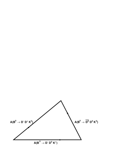
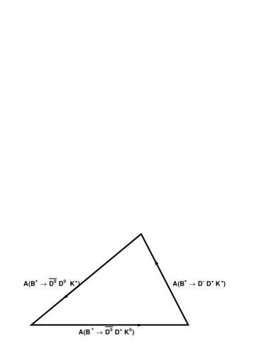
Figure 3: Isospin triangles for the $B^{0}$ (left) and $B^{+}$ (right) amplitudes.

We finally notice that Eq. 6 to 13 are valid not only for the total decay amplitude but also for each helicity amplitude separately as well as for the amplitude as a function of the Dalitz plot coordinates.

3 Study of experimental results

The branching fractions for the charged and neutral $B$ meson decay can be written

$$Br(B^{+}\rightarrow f^{+}) = \tau_{+}\frac{1}{(2\pi)^{3}~{}32M_{B}^{3}}\left(\int dm^{2}_{D\bar{D}}dm^{2}_{DK}\right)|A(B^{+}\rightarrow f^{+})|^{2}$$ (14)

$$Br(B^{0}\rightarrow f^{0}) = \tau_{0}\frac{1}{(2\pi)^{3}~{}32M_{B}^{3}}\left(\int dm^{2}_{D\bar{D}}dm^{2}_{DK}\right)|A(B^{0}\rightarrow f^{0})|^{2},$$ (15)

where $\tau_{+}=2.543\times 10^{12}~{}{\rm GeV^{-1}}$ and $\tau_{0}=2.343\times 10^{12}~{}{\rm GeV^{-1}}$ [11] are the lifetimes of the $B^{+}$ and $B^{0}$ mesons, $M_{B}$ is the mass of the B meson averaged over $B^{0}$ and $B^{+}$, $m_{D\bar{D}}$ and $m_{DK}$ are the invariant masses of the ${D\bar{D}}$ and ${DK}$ subsystem, and the integral is computed numerically over the allowed region of the three-body phase space. In computing these integrals the small mass differences between neutral and charged states for the $B$, $D^{*}$, $D$ and $K$ mesons have been neglected.

The BABAR collaboration has recently studied the full set of $B\rightarrow\kern 1.99997pt\overline{\kern-1.99997ptD}{}^{(*)}D^{(*)}K$ decays and has provided a measurement, reported in Table 1, for all these modes [8]. These data, the most precise to date, have been obtained at the PEP-II accelerator from the reaction $e^{+}e^{-}\rightarrow\mathchar 28935\relax(4S)\rightarrow B\overline{B}$. To compute the branching fractions it has been assumed that $Br(\mathchar 28935\relax(4S)\rightarrow B^{+}B^{-})=Br(\mathchar 28935\relax(4S)\rightarrow B^{0}\kern 1.79993pt\overline{\kern-1.79993ptB}{}^{0})=0.5$. However these equalities do not necessarily hold. In order to account for this factor, we have rewritten equations 14 and 15 in term of the rescaled amplitudes $\tilde{A}=\frac{A}{\sqrt{2b_{0}}}$ where $b_{0}=Br(\mathchar 28935\relax(4S)\rightarrow B^{0}\kern 1.79993pt\overline{\kern-1.79993ptB}{}^{0})$. The expression for $Br(B^{+}\rightarrow f^{+})$ is then multiplied by the additional factor $f_{+/0}=\frac{Br(\mathchar 28935\relax(4S)\rightarrow B^{+}B^{-})}{Br(\mathchar 28935\relax(4S)\rightarrow B^{0}\kern 1.25995pt\overline{\kern-1.25995ptB}{}^{0})}$.

The experimental data have been fitted simultaneously using the $\chi^{2}$ method where the fitted parameters are $f_{+/0}$ and for each set of decays $|\tilde{A_{1}}|$, $|\tilde{A_{0}}|$ and $\delta=arg(\tilde{A_{1}}\tilde{A_{0}^{*}})$. The total number of fitted parameters is 13. The results of the fit are reported in Tables 1 and 2. The overall agreement between the measured and predicted branching fractions is good as can be judged from Table 1, Fig. 4 and from the value $\chi^{2}=8.8$ for 9 degrees of freedom ($n_{dof}$). For this fit the statistical and systematical errors from Ref. [8] have been combined quadratically. This neglects the correlation between the systematical errors (common efficiencies, submode branching fractions, etc.). For some $B^{0}$ decays only the sum of the branching fraction with the charge conjugate final state has been measured. We present in Table 3 the fitted values for the individual branching fractions.

An alternative way of displaying the experimental results and the fit results is given by the isospin triangles introduced above. For ease of comparison, we have normalized the triangles to the size of the basis ($|A(B^{0}\rightarrow D^{(*)-}D^{(*)0}K^{+})|$ and $|A(B^{+}\rightarrow D^{(*)0}D^{(*)+}K^{0})|$): therefore the lower side extends in each case from (0,0) to (1,0) and the shapes of the triangles can be directly compared. Given that we have only a measurement of the sides, there is a fourfold ambiguity on the vertex of the triangle. We have consistently chosen the same solution for its orientation. The seven measured triangles defined in this way are shown in Fig. 5 together with the fit result.

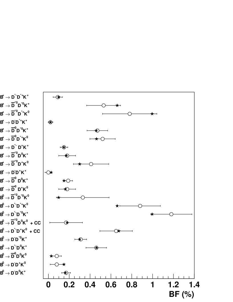
Figure 4: Results of the $\chi^{2}$ fit to the experimental branching fractions. The fitted branching fractions are shown by the stars while the points with error bars show the measured values.

Table 1: Branching fractions (BF) for each $B\rightarrow\kern 1.99997pt\overline{\kern-1.99997ptD}{}^{(*)}D^{(*)}K$ mode. The first error on each branching fraction is the statistical uncertainty and the second is the systematic uncertainty from [8]. The last column presents the result of the $\chi^{2}$ fit.

$B$ decay mode	BF exp. $(\%)$	BF fit $(\%)$
$B^{0}$ decays through external $W$-emission amplitudes
$B^{0}\rightarrow D^{-}D^{0}K^{+}$	$0.17\pm 0.03\pm 0.03$	0.174
$B^{0}\rightarrow D^{-}D^{*0}K^{+}$	$0.46\pm 0.07\pm 0.07$	0.495
$B^{0}\rightarrow D^{*-}D^{0}K^{+}$	$0.31^{+0.04}_{-0.03}\pm 0.04$	0.321
$B^{0}\rightarrow D^{*-}D^{*0}K^{+}$	$1.18\pm 0.10\pm 0.17$	1.065
$B^{0}$ decays through external+internal $W$-emission amplitudes
$B^{0}\rightarrow D^{-}D^{+}K^{0}$	$0.08^{+0.06}_{-0.05}\pm 0.03$	$0.161$
$B^{0}\rightarrow D^{*-}D^{+}K^{0}+D^{-}D^{*+}K^{0}$	$0.65\pm 0.12\pm 0.10$	0.676
$B^{0}\rightarrow D^{*-}D^{*+}K^{0}$	$0.88^{+0.15}_{-0.14}\pm 0.13$	0.707
$B^{0}$ decays through internal $W$-emission amplitudes
$B^{0}\rightarrow\kern 1.99997pt\overline{\kern-1.99997ptD}{}^{0}D^{0}K^{0}$	$0.08\pm 0.04\pm 0.02$	$0.029$
$B^{0}\rightarrow\kern 1.99997pt\overline{\kern-1.99997ptD}{}^{0}D^{*0}K^{0}+\kern 1.99997pt\overline{\kern-1.99997ptD}{}^{*0}D^{0}K^{0}$	$0.17^{+0.14}_{-0.13}\pm 0.07$	0.181
$B^{0}\rightarrow\kern 1.99997pt\overline{\kern-1.99997ptD}{}^{*0}D^{*0}K^{0}$	$0.33^{+0.21}_{-0.20}\pm 0.14$	$0.105$
$B^{+}$ decays through external $W$-emission amplitudes
$B^{+}\rightarrow\kern 1.99997pt\overline{\kern-1.99997ptD}{}^{0}D^{+}K^{0}$	$0.18\pm 0.07\pm 0.04$	$0.163$
$B^{+}\rightarrow\kern 1.99997pt\overline{\kern-1.99997ptD}{}^{*0}D^{+}K^{0}$	$0.41^{+0.15}_{-0.14}\pm 0.08$	$0.300$
$B^{+}\rightarrow\kern 1.99997pt\overline{\kern-1.99997ptD}{}^{0}D^{*+}K^{0}$	$0.52^{+0.10}_{-0.09}\pm 0.07$	0.462
$B^{+}\rightarrow\kern 1.99997pt\overline{\kern-1.99997ptD}{}^{*0}D^{*+}K^{0}$	$0.78^{+0.23}_{-0.21}\pm 0.14$	0.995
$B^{+}$ decays through external+internal $W$-emission amplitudes
$B^{+}\rightarrow\kern 1.99997pt\overline{\kern-1.99997ptD}{}^{0}D^{0}K^{+}$	$0.19\pm 0.03\pm 0.03$	0.150
$B^{+}\rightarrow\kern 1.99997pt\overline{\kern-1.99997ptD}{}^{*0}D^{0}K^{+}$	$0.18^{+0.07}_{-0.06}\pm 0.04$	$0.172$
$B^{+}\rightarrow\kern 1.99997pt\overline{\kern-1.99997ptD}{}^{0}D^{*0}K^{+}$	$0.47\pm 0.07\pm 0.07$	0.459
$B^{+}\rightarrow\kern 1.99997pt\overline{\kern-1.99997ptD}{}^{*0}D^{*0}K^{+}$	$0.53^{+0.11}_{-0.10}\pm 0.12$	0.660
$B^{+}$ decays through internal $W$-emission amplitudes
$B^{+}\rightarrow D^{-}D^{+}K^{+}$	$0.00\pm 0.03\pm 0.01$	$0.027$
$B^{+}\rightarrow D^{-}D^{*+}K^{+}$	$0.02\pm 0.02\pm 0.01$	$0.020$
$B^{+}\rightarrow D^{*-}D^{+}K^{+}$	$0.15\pm 0.03\pm 0.02$	0.149
$B^{+}\rightarrow D^{*-}D^{*+}K^{+}$	$0.09\pm 0.04\pm 0.02$	$0.098$

Table 2: Results of the $\chi^{2}$ fit to the experimental branching fractions. The superscripts $LL$, $L*$, $*L$ and $**$ are for the $B\rightarrow\kern 1.99997pt\overline{\kern-1.99997ptD}{}DK$, $B\rightarrow\kern 1.99997pt\overline{\kern-1.99997ptD}{}D^{*}K$, $B\rightarrow\kern 1.99997pt\overline{\kern-1.99997ptD}{}^{*}DK$ and $B\rightarrow\kern 1.99997pt\overline{\kern-1.99997ptD}{}^{*}D^{*}K$ decays respectively. The amplitude values are in units of $10^{-5}$ while the phases $\delta$ are in degrees. The last column presents the results of the fit introducing a constraint related to other measurements of $f_{+/0}$.

parameter	value	value
$|\tilde{A}_{1}^{LL}|$	$0.28\pm 0.13$	$0.25\pm 0.13$
$|\tilde{A}_{0}^{LL}|$	$0.75\pm 0.07$	$0.73\pm 0.06$
$\delta^{LL}$	$95\pm 22$	$100\pm 23$
$|\tilde{A}_{1}^{L*}|$	$0.27\pm 0.15$	$0.25\pm 0.11$
$|\tilde{A}_{0}^{L*}|$	$1.51\pm 0.11$	$1.45\pm 0.09$
$\delta^{L*}$	$91\pm 34$	$98\pm 36$
$|\tilde{A}_{1}^{*L}|$	$0.75\pm 0.10$	$0.69\pm 0.08$
$|\tilde{A}_{0}^{*L}|$	$1.00\pm 0.11$	$0.99\pm 0.10$
$\delta^{*L}$	$111\pm 17$	$116\pm 14$
$|\tilde{A}_{1}^{**}|$	$0.71\pm 0.17$	$0.66\pm 0.14$
$|\tilde{A}_{0}^{**}|$	$2.38\pm 0.17$	$2.27\pm 0.14$
$\delta^{**}$	$127\pm 26$	$133\pm 22$
$f_{+/0}$	$0.86\pm 0.13$	$1.02\pm 0.05$
$\chi^{2}/n_{dof}$	8.8/9	10.4/10
$Prob(\chi^{2},n_{dof})$	0.456	0.406

Table 3: Fitted values of the branching fractions for the $B\rightarrow\kern 1.99997pt\overline{\kern-1.99997ptD}{}D^{*}K$ and $B\rightarrow\kern 1.99997pt\overline{\kern-1.99997ptD}{}^{*}DK$ decays which have not been measured individually.

$B$ decay mode	BF fit $(\%)$
$B^{0}\rightarrow D^{*-}D^{+}K^{0}$	0.185
$B^{0}\rightarrow D^{-}D^{*+}K^{0}$	0.491
$B^{0}\rightarrow\kern 1.99997pt\overline{\kern-1.99997ptD}{}^{*0}D^{0}K^{0}$	0.160
$B^{0}\rightarrow\kern 1.99997pt\overline{\kern-1.99997ptD}{}^{0}D^{*0}K^{0}$	0.021

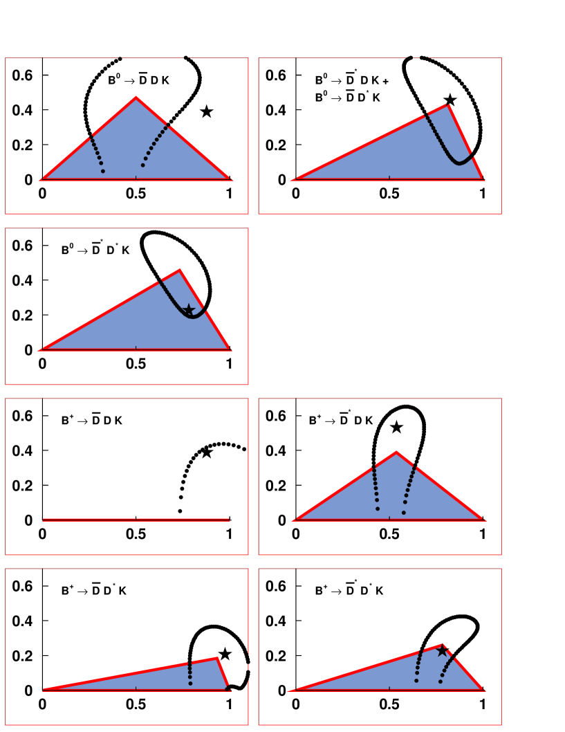
Figure 5: Isospin triangles for the $B\rightarrow\kern 1.99997pt\overline{\kern-1.99997ptD}{}^{(*)}D^{(*)}K$ amplitudes. Each panel presents the measured vertex of the triangle, where the basis has been normalized to unity. The dotted contour shows the one standard deviation region. The star shows the result of the fit. We notice that only one triangle degenerates into a segment while in all the other cases the shape of the triangle presents large angles.

4 Discussion

4.1 The value of $f_{+/0}$ and the validity of isospin relations

The value of $f_{+/0}$ returned by the fit is

$$f_{+/0}=0.86\pm 0.13.$$ (16)

This value is in agreement with the theoretical predictions for $f_{+/0}$ which lie in the 1.05-1.18 interval [12], as well as with other determinations of this quantity: $f_{+/0}=1.04\pm 0.07\pm 0.04$ [2] and $f_{+/0}=1.10\pm 0.06\pm 0.05$ [13] derived from similar isospin relations for the branching fractions of $B$ decays to charmonium final states. Combining these measurements obtained in $B\rightarrow J/\Psi K$ decays, rescaled using the value $\tau_{+}/\tau_{0}=1.083\pm 0.017$ [11], we obtain $f_{+/0}=1.046\pm 0.056$. We have added this constraint to the fit to the data obtaining the result shown in the last column of Table 2. We notice that the measurement presented here does not improve substantially the uncertainty on $f_{+/0}$ and that the values and uncertainties on the amplitudes and phases do not change significantly using this constraint.

The point can be investigated further. The inspection of Fig. 4 and Table 1 shows that the branching fractions for $B\rightarrow\kern 1.99997pt\overline{\kern-1.99997ptD}{}^{*}D^{*}K$ decays deviate from the fitted values in a correlated way. We have repeated the fit separately for the three groups of decays final states obtaining the values for $f_{+/0}$ shown in Table 4. We notice that the value measured in $B\rightarrow\kern 1.99997pt\overline{\kern-1.99997ptD}{}^{*}D^{*}K$ decays deviates from the experimental value in $B\rightarrow J/\Psi K$ decays by 2.95 standard deviations.

Table 4: Values of $f_{+/0}$ for the different groups of decay final states.

final states	$f_{+/0}$
$B\rightarrow\kern 1.99997pt\overline{\kern-1.99997ptD}{}DK$	$1.24\pm 0.43$
$B\rightarrow\kern 1.99997pt\overline{\kern-1.99997ptD}{}^{*}DK+B\rightarrow\kern 1.99997pt\overline{\kern-1.99997ptD}{}D^{*}K$	$1.01\pm 0.21$
$B\rightarrow\kern 1.99997pt\overline{\kern-1.99997ptD}{}^{*}D^{*}K$	$0.55\pm 0.16$

This discrepancy can be explained either by an additional systematical effect in these measurements or by a violation of the isospin symmetry for these final states. Clearly more data are needed to clarify this point. A high precision test of the isospin relations will only be possible when $f_{+/0}$ will be measured using a different experimental method. The large data sample accumulated by the BABAR and BELLE experiments will allow this measurement in the near future.

4.2 Dynamical features of the amplitudes

The amplitudes and phases extracted from the data present some distintive features. First, within each set, the amplitude related to the color-suppressed decays is much smaller, as expected. The ratios $A_{0}/A_{1}$ are presented in Table 5. These ratios, except for the case of $B\rightarrow\kern 1.99997pt\overline{\kern-1.99997ptD}{}^{*}DK$, are close to the naïve expectation $|A_{0}|/|A_{1}|=N_{c}=3$, where $N_{c}$ is the number of colors.

Second, the central values for the relative phases $\delta$ are in all cases close to $90^{\rm o}$. The errors on these values given in Table 2 are not relevant to determine confidence intervals because of the non-linear relation between $\delta$ and $\cos(\delta)$ which enters the $\chi^{2}$ expression. To do this the $\chi^{2}$ profile has been studied keeping in turn one phase $\delta$ fixed and repeating the fit. The 90% level confidence intervals are $92^{\rm o}<\delta^{*L}<154^{\rm o}$ and $88^{\rm o}<\delta^{**}<180^{\rm o}$ while no bound can be set for $\delta^{LL}$ and $\delta^{L*}$. The superscripts $LL$, $L*$, $*L$ and $**$ are for the $B\rightarrow\kern 1.99997pt\overline{\kern-1.99997ptD}{}DK$, $B\rightarrow\kern 1.99997pt\overline{\kern-1.99997ptD}{}D^{*}K$, $B\rightarrow\kern 1.99997pt\overline{\kern-1.99997ptD}{}^{*}DK$ and $B\rightarrow\kern 1.99997pt\overline{\kern-1.99997ptD}{}^{*}D^{*}K$ decays respectively. From this we can conclude that there is a reasonable indication for large strong phases in these amplitudes. This suggests the presence of non-negligible Final State Interaction for these decays. This is both an important indication per se and has also consequences for the CP violation studies that will be discussed in the next section.

Table 5: Ratios $A_{0}/A_{1}$ from the fit to the data.

ratio	value
$|A_{0}^{LL}|/|A_{1}^{LL}|$	$2.68\pm 2.44$
$|A_{0}^{L*}|/|A_{1}^{L*}|$	$5.59\pm 2.04$
$|A_{0}^{*L}|/|A_{1}^{*L}|$	$1.33\pm 0.24$
$|A_{0}^{**}|/|A_{1}^{**}|$	$3.35\pm 0.98$

4.3 Implications for a $\sin(2\beta)$, $\cos(2\beta)$ measurement

All the $B^{0}\rightarrow\kern 1.99997pt\overline{\kern-1.99997ptD}{}^{*}D^{*}K^{0}$ are in principle good candidates for the measurement of $\beta$. In the past the emphasis has been placed on the $B^{0}\rightarrow\kern 1.99997pt\overline{\kern-1.99997ptD}{}^{*}D^{*}K^{0}$ and $B^{0}\rightarrow\kern 1.99997pt\overline{\kern-1.99997ptD}{}^{*}D^{*}K^{0}$ decays [4, 5, 6] and preliminary theoretical values of the branching fractions have been presented. We notice that the values for the branching fractions of these modes presented in Tables 1 and 3 can be used for more precise assessments of the sensitivity of a measurement of $\beta$ using these modes.

In Ref.[8], the observation of the modes $B^{0}\rightarrow D^{*-}D^{*+}K^{0}$ and $B^{0}\rightarrow D^{-}D^{*+}K^{0}+CC$ is reported. We notice that for $B^{0}\rightarrow D^{*-}D^{*+}K^{0}$, the measured value of the branching fraction ($0.88^{+0.15}_{-0.14}\pm 0.13$) and the value predicted by our fit ($0.707$) are almost a factor two lower that what anticipated in Ref. [6], thereby unfortunately also reducing the comparative advantage of this mode with respect $B^{0}\rightarrow D^{*-}D^{*+}$.

For $B^{0}\rightarrow D^{-}D^{+}K^{0}$, Ref. [8] reports only a 90% CL upper limit (0.17 %) which is very close to the fitted value 0.161 %. This means that the observation of this mode in the near future is possible. The estimated value of Ref. [5] ($9~{}10^{-3}$) is a factor 6 above our predicted value. We stress that this channel is a good candidate for CP-violation studies because of the nature of the final state with three pseudoscalar particles. This will facilitate the angular analysis to determine the helicity amplitudes.

Finally we stress that the $B^{0}\rightarrow D^{*-}D^{+}K^{0}$ and $B^{0}\rightarrow D^{-}D^{*+}K^{0}$ lead to final states accessible by both $B^{0}$ and $\kern 1.79993pt\overline{\kern-1.79993ptB}{}^{0}$. They can therefore be analysed in the same way as described in Ref.[14]. The strong phases play an important role for this analysis as the time-dependent CP-asymmetry amplitudes are proportional to $\sin(2\beta\pm\delta^{\prime})$, where $\delta^{\prime}$ is the strong phase difference between $A(B^{0}\rightarrow D^{-}D^{*+}K^{0})$ and $A(\kern 1.79993pt\overline{\kern-1.79993ptB}{}^{0}\rightarrow D^{-}D^{*+}K^{0})$. The possibly large values of the strong phases noticed above need to be taken into account for any estimate of the sensitivities of this analysis.

5 Conclusion

We have presented the complete isospin relations for the $B\rightarrow\kern 1.99997pt\overline{\kern-1.99997ptD}{}^{(*)}D^{(*)}K$ decays. These relations have been compared to the recent experimental measurements through a fit of the isospin amplitudes. The overall agreement between the measured and the expected branching fractions is good with the exception of a possible discrepancy for the $B\rightarrow\kern 1.99997pt\overline{\kern-1.99997ptD}{}^{*}D^{*}K$ decays. The isospin amplitudes present several peculiar features which point to a dynamical origin. Large values of the strong phases are suggested by the data. We have also presented a new measurement of $\frac{Br(\mathchar 28935\relax(4S)\rightarrow B^{+}B^{-})}{Br(\mathchar 28935\relax(4S)\rightarrow B^{0}\kern 1.25995pt\overline{\kern-1.25995ptB}{}^{0})}=0.86\pm 0.13$ in agreement with other determinations of this quantity. The implications of these results for the measurement of $\sin(2\beta)$ and $\cos(2\beta)$ using these decays have been discussed.

6 Acknowledgments

The author wishes to warmly thank J. Charles, J.P. Lees and L. Oliver for reading the manuscript and making useful suggestions.

References

• [1] H.J. Lipkin and A. I. Sanda, Phys. Lett. B 201, 541 (1988).
• [2] CLEO Collaboration, J.P. Alexander et al., Phys. Rev. Lett. 86, 2737 (2001).
• [3] G. Buchalla, I. Dunietz and H. Yamamoto, Phys. Lett. B 364, 185 (1995).
• [4] J.Β Charles, A.Β Le Yaouanc, L.Β Oliver, O.Β PΓ¨ne, and J.C.Β Raynal, Phys. Lett. B 425, 375 (1998) [Erratum-ibid.Β B 433, 441 (1998)].
• [5] P.Β Colangelo, F.Β De Fazio, G.Β Nardulli, N.Β Paver and Riazuddin, Phys. Rev. D 60, 033002 (1999).
• [6] T.E.Β Browder, A.Β Datta, P.J.Β O’Donnell and S.Β Pakvasa, Phys. Rev. D 61, 054009 (2000).
• [7] CLEO Collaboration, CLEO CONF 97-26, EPS97 337 (1997). Aleph Collaboration, R. Barate et al., Eur. Phys. Jour. C 4, 387 (1998). Belle Collaboration, K. Abe et al., BELLE-CONF-0104 (2001).
• [8] BABAR Collaboration, B. Aubert et al., Phys. Rev. D 68, 092001 (2003).
• [9] M. Peshkin and J.L. Rosner, Nucl. Phys. B 122, 144 (1977).
• [10] C.W. Bauer, B. Grinstein, D. Pirjol and I.W. Stewart, Phys. Rev. D 67, 014010 (2003).
• [11] Particle Data Group, K. Hagiwara et al., Phys. Rev. D 66, 010001 (2002).
• [12] D. Atwood and W. Marciano, Phys. Rev. D 41, 1736 (1990). N. Byers and E. Eichten, Phys. Rev. D 42, 3885 (1990). P. Lepage, Phys. Rev. D 42, 3251 (1990).
• [13] BABAR Collaboration, B. Aubert et al., Phys. Rev. D 65, 032001 (2002).
• [14] R. Aleksan et al., Nucl. Phys. B 361, 141 (1991).