Abstract

Modelling Quark-Gluon Plasma formation and decay in high energy heavy ion reactions is presented in a framework of a multi-module setup. The collective features, governing the equlibrated fluid dynamical stages of the model are emphasized. Flow effects formed from the initial conditions are discussed. Particular attention is given to the improvement of the final hadronization and freeze-out part of the reaction which has strong effects on the observables.

[Phase Transitions in High Energy
Heavy-Ion Collisions] Phase Transitions in High Energy
Heavy-Ion Collisions

Phase Transitions in …

1 Introduction

Phase Transitions imply that we have different phases of the matter we deal with, and it has an Equation of State (EoS). We can have an EoS if and only if the matter is in statistical equilibrium, or at least close to it. When this condition is satisfied we can apply a fluid- and thermodynamical description for the dynamics of the system. In high energy heavy ion reactions we observe many thousand particles produced in the reaction, so, we have all reasons to assume that in a good part of the reaction the conditions of the local equilibrium and continuum like behaviour are satisfied.

The initial and final stages are, on the other hand, obviously not in statistically equilibrated states, and must be described separately, in other theoretical approaches. The different approaches, as they describe different space-time (ST) domains and the corresponding approaches can be matched to each other across ST hyper-surfaces or across some transitional layers or fronts. The choice of realistic models at each stage of the collision, as well as the correct coupling of the different stages or calculational modules are vital for a reliable reaction model. The most basic requirements are that conserved quantities should stay conserved when modules are interfaced to each other, and entropy should not decrease.

For the theoretical description and understanding of high energy heavy ion collisions it is important to mention that while our system is sufficiently large to assume statistical equilibrium, it is not a macroscopic system with Avogadro number of particles. We deal with a small, mesoscopic system, so discontinuities of the thermodynamical quantities, will not be observable, but at the same time the changes are sudden and rapid enough that they can be recognized.

The other basic feature of mesoscopic systems is also important to us: in such systems fluctuations are not negligible but dominant, these can be observed and these may help to identify the properties of the phase transition.

Dividing the reaction model into standardized modules and interfaces leads to additional advantages. Modules can be replaced easily, research groups can collaborate better and the GRIDS of High Performance Computers can increase the speed of complete reaction simulation by about an order of magnitude.

2 Initial Stage Module

Many fluid dynamical approaches use simple parametrizations for the initial state of the hydrodynamic stage with a few parameters. These can then be fitted or adjusted by comparing experimental data and model predictions.

A more physical approach is to start from a dynamical, pre-equilibrium model, e.g. Parton Cascade Model (PCM), or Collective (or Coherent) Yang-Mills model, or different versions of flux-tube models.

Our recent works are based on a latter type of approach [1], which was implemented in a Fire-Streak geometry streak by streak and upgraded to satisfy energy, momentum and baryon charge conservations exactly at given finite energies [2, 3]. The effective string-tension was different for each streak, stretching in the beam direction, so that central streaks with more color (and baryon) charges at their two ends had bigger string-tension and expanded less, than peripheral streaks. The expansion of the streaks was assumed to last until the expansion has stopped. Yo-yo motion, as known from the Lund-model was not assumed.

In the 1st version of the model at full stopping of string expansion, the baryon charge was distributed uniformly along each streak. This created an initial state for the hydrodynamic stage where each streak was stopped in its own CM frame, and had uniform baryon and energy density distribution. The sharp forward and backward end led, however, to a development of a large, Fwd/Bwd density peaks. [4]

Thus, we concluded that the assumption of uniform distribution and sharp cuts at the ends is overly simplified and has to be corrected. So, a Fwd/Bwd expansion was added to the model [3], which smoothed the Fwd/Bwd ends, and eliminated the artificial large, Fwd/Bwd density peaks.

Our calculations show that such a tilted initial state leads to the creation of of the third flow component [5], peaking at rapidities $|y|\approx 0.75$ [4]. Recent, STAR $v_{1}$ data [6] indicate that our assumption that the string expansion lasts until full stopping of each streak, may also be too simple and local equilibration may be achieved earlier, i.e. before the full uniform stopping of a streak. We did not explicitly calculate dissipative processes, some friction within and among the expanding streaks is certainly present and experiments seem to indicate that this friction is stronger.

3 Relativistic Fluid Dynamics

When parts of our system reach local statistical equilibrium in the ST, following a pre-equilibrium development, we can describe our system using Computational FLuid Dynamics (CFD) and an Equation of State. The equations of Fluid Dynamics (FD) can be most simply derived from the Boltzmann Transport Equation (BTE).

The relativistic BTE below, describes the time evolution of the single particle distribution function based on the assumptions that just two particle collisions are considered (binary collisions), the number of binary collisions at $x$ is proportional to $f(x,p_{1})\times$ $f(x,p_{2})$ and $f(x,p)$ is a smoothly varying function compared to mean free path. So, one can show that BTE has the form [see Chapter 3 of ref. [7]] :

$$p_{k}^{\mu}f_{k,\mu}=\sum_{l=1}^{N}C_{kl}(x,p_{x})$$

where $C$ is the collision integral, and $k$ and $l$ stand for different particle species or particle components. Then, using microscopic conservation laws in the collision integral, from the BTE we can derive the differential form of conservation laws [see section 3.6 of ref. [7]]:

$$N_{,\mu}^{\mu} = \sum_{k=1}^{N}N_{k,\mu}^{\mu}=0\rm{\ \ \ \ :conservation\ of\ particle\ number}$$ (1)

$$Q_{,\mu}^{\mu} = \sum_{k=1}^{N}Q_{k,\mu}^{\mu}=0\rm{\ \ \ :conservation\ of\ charge}$$ (2)

$$T_{,\mu}^{\mu\nu} = \sum_{k=1}^{N}T_{k,\mu}^{\mu\nu}=0\rm{\ \ :conservation\ of\ energy\ and\ momentum}$$ (3)

where _,μ denotes $\partial/\partial\mu$ and there is a summation for indexes occurring twice. These equations are valid for any distribution satisfying the BTE. These equations can be used if we know the solution and then we can evaluate the conserved quantities.

3.1 Perfect and Viscous Fluids

Equations (1-3) are also the equations of FD. But these equations must not be considered as consequences of BTE, rather these equations are postulated, as the differential forms of conservation laws. This can be done because such conservation laws can be derived from other theoretical approaches also.

These equations are not a closed set, because the energy momentum tensor and the particle four current should also be defined. In the Eulerian or perfect fluid dynamics we postulate the form of energy-momentum tensor, and an EoS, $P=P(e,n)$, must be given. This provides a closed set of partial differential equations that is solvable. Any EoS, which is consistent with thermodynamics, can be used. One does not have to assume dilute systems with binary collisions, or the assumption of molecular chaos. The only requirement is the existence of local equilibrium, otherwise we would not have an EoS.

In the case of Navier-Stokes fluid dynamics, we assume that the energy momentum tensor also contains the dissipative part $T^{\mu\nu(1)}$, which allows for small, first order deviations from local equilibrium. Thus, to have a solution we need not only the EoS, but also the transport coefficients that occur in the dissipative part of the energy-momentum tensor.

Boltzmann’s H-theorem implies that if irreversible processes are present the entropy increases. In equilibrium the distribution is constant, the entropy is also constant, but it reached its maximum value.

It is important to know that this can be seen from fluid dynamics also. In perfect fluid dynamics the flow is adiabatic, no entropy is produced. This can be proven using the equations of perfect fluid dynamics and standard thermodynamical relations. Entropy production is strictly, and quantitatively connected to dissipative processes. Perfect flow is adiabatic even in the presence of phase transitions, if the two phases are in thermal, mechanical ($P$), chemical and phase equilibrium all the time! On the other hand if the phase transition deviates from equilibrium this leads to entropy production. See Assignment 9.4.a in ref. [7].

As shock waves, detonations, deflagrations, are idealizations of very sharp or very rapid processes as discontinuities, the above conclusions are valid for discontinuities also. Nevertheless, frequently, dissipative processes can be neglected for most of the flow except the sharp or rapid changes. Thus, as an end effect the dissipative processes are frequently localized in sharp fronts or in hypersurfaces of discontinuities. One should not, however, forget that dissipation is due to transport properties and characteristic constants of phase transition dynamics, even if it happens in ”discontinuities”.

3.2 Equations of Perfect Fluid Dynamics

We assume that our system is not homogeneous, but the gradients are small, so local distribution can be an equilibrium distribution, e.g. a Jüttner distribution. Now the local $n(x),e(x),s(x)$ and $P=P(n,e)$ are known, and we assume that in LR, $T^{\mu\nu}$ is diagonal. Now using the conservation laws with introducing the apparent density as:

$$N\equiv n\gamma\ ,$$

the continuity equation takes the familiar form

$$(\partial_{t}+\mathbf{v}\ \rm{grad})\ N=-M\ \rm{div}\ \mathbf{v}\ ,$$

similarly introducing

$$\mathbf{M} \equiv T^{0i}=w\ \gamma^{2}\mathbf{v}$$ (4)

$$\varepsilon \equiv T^{00}=(e+P\mathbf{v}^{2})\gamma^{2}\ ,$$ (5)

the energy and momentum conservation will take the form

$$(\partial_{t}+\mathbf{v}\ \rm{grad})\mathbf{M} =-\mathbf{M}(\rm{div}\mathbf{v})-\rm{grad}\ P$$ (6)

$$(\partial_{t}+\mathbf{v}\ \rm{grad})\varepsilon =-\varepsilon\ \rm{div}\mathbf{v}-\rm{div}(P\mathbf{v})\ .$$ (7)

Thus to solve the equations of relativistic fluid dynamics we have to solve the same partial differential equations as in the non-relativistic case. We cannot immediately apply the EoS to obtain the solution, as the EoS is given in terms of invariant scalars. So, we have to solve in addition the set of algebraic equations above, which connect $N$, $\mathbf{M}$, and $\varepsilon$ to $n$, $e$, $P$ and $\mathbf{v}$, for every fluid cell at every time step.

Important to note that the relativistic treatment is necessary not only at high velocities (i.e. if $v\sim c$) but also at low velocities when the pressure is not negligible compared to the energy density (i.e., $P\sim e$) as $w=e+P$ appears in the relativistic Euler equation! This is frequently the situation for ultra-relativistic gases, like the Stefan-Boltzmann or photon gas (or radiation pressure) where $P=e/3$. This is actually the indication of the fact that the constituents of the matter move with velocity $c$ or close to it.

In principle the perfect fluid dynamics is absolutely unstable. Any spontaneous deviation from an exact solution, will grow exponentially, as their energy cannot be dissipated away [8]. In other words the Reynolds number tends to infinity and the system tends to turbulence. Viscosity is needed to stabilize the flow.

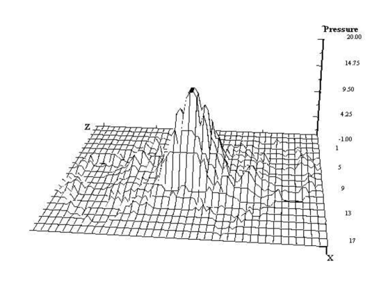
Figure 1: The pressure, in units of [GeV/fm³], in the reaction plane at a late stage (13 fm/c) of a 65+65 Gev/nucl. Au+Au collision, at b=0.5 b-max, using the Bag Model EoS for QGP. The outer, supercooled regions have negative pressure, while in the very center it is still large. The directed flow, is visible as the outside, negative pressure regions in the upper-right and lower-left corners, close to the beam, $Z-$, direction. The third flow component [5] is shown by a smaller negative pressure peak at the lower side of the plot, slightly right of the middle. The section of the reaction plane, [x,z], shown is 12.1 $\times$ 9.6 fm.

There are several numerical methods to obtain a solution. In all cases the solution is discretized in some way and a coarse graining is introduced. This coarse graining automatically leads to dissipative and transport properties, and the parameters of these transport processes can be determined by numerical experiments. The result is that all CFD models are dissipative or viscous, which is an advantage as the these are usually stable. By decreasing the cell size, the dissipative effects can be decreased in CFD, to a limit when instabilities, or turbulence occurs. As a side effect, CFD models lead to entropy production, as part of the kinetic energy is dissipated away due to the coarse graining or smoothing.

4 Kinetic Theory of Particle Formation, Escape and Freeze-out

Most frequently relativistic kinetic theory describes the time, $t$, development of the single particle distribution function, $f(p;x)=f(p,\mathbf{r},t)$, of conserved particles in the 6-dimensional Phase-Space (PS), $[\mathbf{p},\mathbf{r}]$ and time. Then the total particle number does not change with time. We assume (usually) that the particles are on mass shell, so the 4-momentum has 3 independent variables. The phase space distribution is a density in the 6 dimensional PS and it is an invariant scalar, because a Lorentz boost contracts the system in the configuration space but elongates it in the momentum space.

If we want to describe a particle source (or drain) from a matter, the total number of newly crated particles can be given as

$$N_{new}=\int d^{4}p\ d^{4}x\ g(p,x),$$

where $g(p,x)$ is an invariant scalar density in the 4-dimensional PS and 4-dimensional space-time (ST). If the particles are on mass shell the momentum space integral can be reduced to

$$N_{new}=\int\frac{d^{3}p}{p^{0}}\ d^{4}x\ h(p,x),$$ (8)

where $h(p,x)$ is also an invariant scalar density, as $\frac{d^{3}p}{p^{0}}$ is also one.

The particle formation or source density $h(p,x)$ from a matter, can be characterized by 3 factors:
PS distribution, $f(p,\mathbf{r},t)$,
PS emission probability, $P_{esc-PS}(p;x)$,
ST emission probability, $P_{esc-ST}(x;p)$.
Here $f$ can be an arbitrary distribution, but we usually discuss matter in (or close to) statistical equilibrium, with known PS distribution. $P_{esc-PS}$ is most frequently assumed to be unity, while $P_{esc-ST}$ is the ST distribution if the source (e.g. a 4-dimensional Gaussian in the ST). The experimental analysis of two particle correlations from heavy ion reactions, is based on these very simple assumptions in most cases.

These are very strong assumptions. It is not supported by experiments that the emission probability is isotrope and homogeneous in the PS, or neither that the ST distribution of the source is Gaussian.

4.1 Non-isotropic particle sources

Not only in heavy ion reactions but in any dynamical process, particle creation, (or condensation) happens mostly in a directed way: the phenomenon propagates into some direction, i.e. it happens in some (space-like) layer or front (like detonations, deflagrations, shocks, condensation waves or freeze-out). The reason is that neighbouring regions in the front may interact, minimize the energy of the front by evening it out, provide energy to neigbouring regions to exceed the threshold conditions. Even in relativistic processes, that are time-like, (have time-like normal) and the neighbouring points of a front cannot be in causal connection, in the LR frame of the matter the dynamical process may and frequently has a direction. (See the example in ref. [9].)

These fronts or layers are not necessarily narrow, but they have a characteristic direction (or normal, $d^{3}\sigma^{\mu}$), thus the ST integral, $d^{4}x$, can be converted into

$$d^{4}x\longrightarrow ds^{\mu}\ d^{3}\sigma_{\mu}.$$

The front can actually be directed time-like, $d^{3}\sigma^{\mu}\ d^{3}\sigma_{\mu}=+1$, or space-like, $d^{3}\sigma^{\mu}\ d^{3}\sigma_{\mu}=-1$.

An example for emission distributed in the ST, but being time-directed can be described by the expression:

$$N_{new}=\int d^{3}p\int d\tau d^{3}\sigma_{\mu}\ \ f_{eq}(p,x)\ \ \frac{C_{1}p^{\mu}}{p^{0}}\ \Theta(p^{\nu}\ d^{3}\sigma_{\nu})\ \ G\left(\tau-\tau_{FO}(x)\right)$$ (9)

where

$$\frac{C_{1}p^{\mu}}{p^{0}}\ \Theta(p^{\nu}\ d^{3}\sigma_{\nu})\$$ (10)

is the PS emission probability, where the step function eliminates the possibility of emission of particles, in the direction opposite to the normal of the front (for time-like normals it is always $+1$), and the term, $\frac{p^{\mu}}{p^{0}}=(1,\mathbf{v})$, together with the 6- dimensional PS density, $f_{eq}$, yield the generalized 4-dimensional flux of particles with momentum $\mathbf{p}$: $\ \ f_{eq}(p,x)\ \frac{p^{\mu}}{p^{0}}.$

Here $G$ is a Gaussian time distribution or emission density for time-like directed fronts:

$$d\tau\ G(\tau-\tau_{FO})=\frac{d\tau}{\sqrt{2\pi}\ \tau_{coll.}}\exp\left[-\frac{(\tau-\tau_{FO})^{2}}{2\tau^{2}_{coll.}}\right]$$

and for space-like fronts:

$$ds\ G(s-s_{FO})=\frac{ds}{\sqrt{2\pi}\ \lambda_{m.f.p.}}\exp\left[-\frac{(s-s_{FO})^{2}}{2\lambda^{2}_{m.f.p.}}\right]$$

.

In more complex models the emission probabilities may take more realistic and more complicated forms. Furthermore, $f_{e.q.}$ can be space-time dependent, and can be determined self-consistently during the detonation, deflagration or freeze out process [10, 11, 12, 13] .

Let us rewrite the escape probability, (10), with the hyper-surface element, covering both the timelike and spacelike parts of the freeze-out surface,

$$P^{*}_{esc-PS}=\frac{p^{\mu}d^{3}\sigma_{\mu}}{(p^{\nu}u_{\nu})}\ \Theta(p^{\mu}d^{3}\sigma_{\mu}).$$ (11)

Here $d^{3}\sigma_{\mu}(x)$ and $u_{\mu}(x)$ are ST dependent and this yields the secondary $x-$dependence of $P^{*}_{esc-PS}(p;x)$. If we take the four velocity equal to $u_{\mu}=(1,0,0,0)$, in the Rest Frame of the Front (RFF), i.e. where $d^{3}\sigma_{\mu}=(1,0,0,0)$, then $P$ is unity. Otherwise, in the Rest Frame of the Gas (RFG), where $u_{\mu}=(1,0,0,0)$, the escape probability $P$ is $P^{*}_{esc-PS}={p^{\mu}d^{3}\sigma_{\mu}}\ \Theta(p^{\mu}d^{3}\sigma_{\mu})/{p^{0}}.$

Figure 2: A simple FO-surface in the Rest Frame of the Gas (RFG), where $u^{\mu}=(1,0,0,0)$, including time-like and space-like parts. Then the normal vector of the FO front, $d^{3}\sigma_{\mu}(x)$, is time-like at the time-like part and it is changing smoothly into a space-like 4-vector in the space-like part. On these two parts of the hyper-surface, in the Local Rest Frame of the Front (RFF), $d^{3}\sigma_{\mu}(x)$ points into the direction of the $t^{\prime}$ ($x^{\prime}$) axis respectively.

The nominator depends on $d^{3}\sigma_{\mu}$. In the following, we will take different typical values for $d^{3}\sigma_{\mu}$, for characteristic regions (A, B, C, D, E, F) of the freeze-out hyper-surface (see Figure 2):

• A  $d^{3}\sigma_{\mu}=(1,0,0,0)$, leads to $p^{\mu}d^{3}\sigma_{\mu}=p^{0}\geq 0$, as we have seen above for FO along the time axis in RFG,

• B  $d^{3}\sigma_{\mu}=\gamma(a,b,0,0)$,

• C  $d^{3}\sigma_{\mu}=\gamma(1+\epsilon,1-\epsilon,0,0)$, just above the light-cone,

• D  $d^{3}\sigma_{\mu}=\gamma(1-\epsilon,1+\epsilon,0,0)$, just below the light-cone,

• E  $d^{3}\sigma_{\mu}=\gamma(c,d,0,0)$,

• F  $d^{3}\sigma_{\mu}=(0,1,0,0)$, leads to $p^{\mu}d^{3}\sigma_{\mu}=p^{x}$, for FO along the spatial axis $x$ in RFG,

where the $\gamma$ factors serve the unit normalization of the normal vectors (see Figure 2). The effect of this relativistically invariant FO factor leads to a smoothly changing behaviour as the direction of the normal vector changes in RFG (see Figure 2).

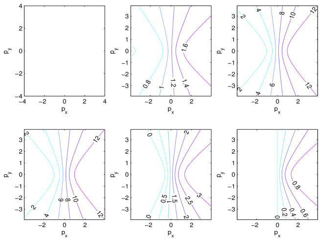
Figure 3: The contour plots of the escape probability factor as function of the particle momentum , $P(\mathbf{p})$, at different points of the FO hyper-surface are presented in six subplots. All plots are in the Rest Frame of the Gas ($RFG$). For region $A$: $d^{3}{\sigma}_{\mu}=(1,0,0,0)$, and the probability factor is one uniformly, for $B$: $d^{3}{\sigma}_{\mu}=\gamma_{\sigma}(1,0.5,0,0)$, $C$ (first row) $D$, $E$: $d^{3}{\sigma}_{\mu}=\gamma_{\sigma}(1,2,0,0)$ $F$: $d^{3}{\sigma}_{\mu}=(0,1,0,0)$ (second row). The momenta are in units of $[mc]$.

To calculate the parameters of the normal vector $d^{3}\sigma_{\mu}$ for different cases listed above, we simply make use of the Lorentz transformation. The normal vector of the time-like part of the freeze-out hypersurface may be defined as the local $t^{\prime}$-axis, while the normal vector for the space-like part may be defined as the local $x^{\prime}$-axis. As the $d^{3}{\sigma}_{\mu}$ normal vector is normalized to unity its components may be interpreted in terms of $\gamma_{\sigma}$ and $v_{\sigma}$, as $d^{3}\sigma_{\mu}=\gamma_{\sigma}(1,v_{\sigma},0,0)$, where $\gamma_{\sigma}=\frac{1}{\sqrt{1-v_{\sigma}^{2}}}$ for time-like normals and $\gamma_{\sigma}=\frac{1}{\sqrt{v_{\sigma}^{2}-1}}$ for space-like normals. This will lead to,

• A  $d^{3}\sigma_{\mu}=(1,0,0,0)$, leads to $P=1$,

• B  $d^{3}\sigma_{\mu}=\gamma_{\sigma}(1,v_{\sigma},0,0)$, leads to $P=\frac{\gamma_{\sigma}(p^{0}+v_{\sigma}p^{x})}{p^{0}}$, and $\gamma_{\sigma}=\frac{1}{\sqrt{1-v^{2}_{\sigma}}}$,

• C  $d^{3}\sigma_{\mu}=\gamma_{\sigma}(1+\epsilon,1-\epsilon,0,0)$, leads to $P=\frac{4\gamma_{\sigma}^{2}(p^{0}+p^{x})+\gamma_{\sigma}(p^{0}+p^{x})}{4\gamma_{\sigma}p^{0}}$,

• D  $d^{3}\sigma_{\mu}=\gamma_{\sigma}(1-\epsilon,1+\epsilon,0,0)$,
  leads to $P=\frac{4\gamma_{\sigma}^{2}(p^{0}+p^{x})-\gamma_{\sigma}(p^{0}-p^{x})}{4\gamma_{\sigma}p^{0}}\times\Theta(p^{\mu}d^{3}\sigma_{\mu})$,

• E  $d^{3}\sigma_{\mu}=\gamma_{\sigma}(1,v_{\sigma},0,0)$,
  leads to $P=\frac{\gamma_{\sigma}(p^{0}+v_{\sigma}p^{x})}{p^{0}}\times\Theta(p^{\mu}d^{3}\sigma_{\mu})$, and $\gamma_{\sigma}=\frac{1}{\sqrt{v^{2}_{\sigma}-1}}$,

• F  $d^{3}\sigma_{\mu}=(0,1,0,0)$, leads to $P=\frac{p^{x}}{p^{0}}\times\Theta(p^{\mu}d^{3}\sigma_{\mu})$, (see Figure 2).

The resulting Phase Space escape probabilities are shown in Figure 3 for the six cases described above.

In refs. [10, 11] the post FO distribution was evaluated for space-like gradual FO in a kinetic model. Initially we had an equilibrated, interacting, PS distribution, $f_{int}(p,x)$, and an escape probability, similar to eq. (11), but simplified so that it depended on the angle of the two vectors only. After some small fraction of particles were frozen out as the FO process progressed in the front, the interacting component were re-equilibrated, with smaller particle number, smaller energy and momentum, to account for the quantities carried away by the frozen out particles. This was then repeated many times in small steps along the FO front and the frozen out particles were accumulated in the post freeze out PS distribution, $f_{free}$. The resulting distribution was highly anisotropic and obviously non-equilibrated. The details of the post FO distribution depend on the details of the escape probability, and on the level of re-equilibration of the remaining, interacting component.

Bugaev assumed earlier [14], that the post FO distribution is a (sharply) ”Cut-Juttner” distribution, but the above mentioned model shows that this can only be obtained if re-equilibration is not taking place. The kinetic model provided an asymmetric but smooth PS distribution [10], while the escape probability (11) yields a somewhat different, but also smooth PS distribution. These can be well approximated by the ”Cancelling Juttner” distribution [15], Figure 4.

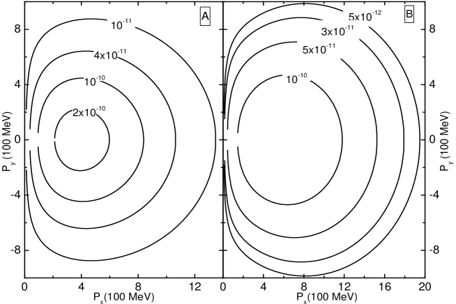
Figure 4: A simple FO-surface in the Rest Frame of the Gas (RFG) where $d^{3}\sigma_{\mu}=(1,0,0,0)$, including timelike and spacelike parts. Then $d^{3}\sigma_{\mu}$ is $t^{\prime}=d^{3}\sigma_{\mu}$ for the timelike part, changing smoothly into $x^{\prime}=d^{3}\sigma_{\mu}$ for spacelike normal vectors.

Up to now we analysed the FO probability in the momentum space only. At this point we should also mention, that if we discuss gradual FO across a finite layer, the distance from a hypothetical or theoretical FO surface must also be part of the FO probability, because the probability of a particle has no more collision on its way out depends on the local mean free path (m.f.p.) and on the distance from this surface. The m.f.p. is usually momentum dependent and this yields the secondary $p-$dependence of $P_{esc-ST}(x;p)$. Of course the position of such a hypothetical FO surface has to be determined self consistently or within a realistic kinetic model. However, if we assume simultaneous FO and hadronization [16, 17] from supercooled plasma, there are no realistic and reliable dynamical models up to know, which we could use, so, a now the first self consistent approximate method is our only choice.

4.2 Emission on an idealized hyper-surface

If the m.f.p. or the coll. time are negligibly small compared to the ST dimensions of the system we can idealize the source distribution further as the source is shrinking to a hyper-surface (HS) in the ST, i.e.:

$$\frac{d\tau}{\sqrt{2\pi}\ \tau_{coll.}}\exp\left[-\frac{(\tau-\tau_{FO})^{2}}{2\tau^{2}_{coll.}}\right]\longrightarrow\delta(\tau-\tau_{FO})\ d\tau\ {\rm:time-like\ fronts,}$$

$$\frac{ds}{\sqrt{2\pi}\ \lambda_{m.f.p.}}\exp\left[-\frac{(s-s_{FO})^{2}}{2\lambda^{2}_{m.f.p.}}\right]\longrightarrow\delta(s-s_{FO})\ ds\ {\rm:space-like\ fronts,}$$

and the integration in the normal direction to the front can be executed. Then

$$N_{new}=\int\frac{d^{3}p}{p^{0}}\ \int_{\Sigma}\ (p^{\mu}d^{3}\sigma_{\mu})\ \Theta(p^{\mu}\ d^{3}\sigma_{\mu})\ f_{FO}(p,x)\ C_{1}\ .$$ (12)

Here _Σ denotes integration over a 3-dimensional HS. If all particles described by $f_{e.q.}$ are emitted during the process, $C_{1}=1$. If we do not perform the momentum integral we recover the modified ”Cooper-Frye” freeze out formula[18, 14, 19]

$$p^{0}\frac{dN}{d^{3}p}=\int_{\Sigma}p^{\mu}d^{3}\sigma_{\mu}\ \Theta(p^{\mu}\ d^{3}\sigma_{\mu})\ f_{FO}(p,x)$$ (13)

Notice that we have changed the notation of the PS distribution from $f_{eq}$ to $f_{FO}$ denoting the post FO distribution integrated across the front.

Eq. (13) simplifies the process to a great extent, especially if we consider that $f_{eq}$ changes during the detonation deflagration or freeze out process as we go across the front self-consistently. In a dynamical process across the front, even if $f_{eq}$ is always an equilibrated distribution, its parameters change in a wide range [10, 11]. In the FO process the post FO distribution, after the process is completed is very far from any statistically equilibrated distribution. This should be taken into account if we apply the assumption of an idealized FO surface. The determination of the FO surface is an involved task, both physically and technically. In complex modeling tasks we perform the self-consistent determination of the surface in simplified models. In these models we can pinpoint the FO conditions and evaluate the post FO distributions.

Then based on this knowledge we determine the FO surface in the large scale, 3+1 dimensional system by analysing the complete ST history of the fluid dynamical stage calculated. This demanding task was completed recently by Bernd R. Schlei (of Los Alamos) [20], and this enables us to visualize the ST evolution of the surface where the emitted particles originate from.

5 Two particle correlations

In case of two particle correlations we have to return to eqs. (8) or (9), because the emission point in ST is crucial. Although, eqs. (12) or (13) also contain a ST dependence, this is reflecting the properties of the idealized hypersurface, where the process is taking place. This approximation is justified only if

• The ST domain of the emission is a negligibly narrow layer and we are sure that the internal processes within the front are not relevant.

• If we use a realistic estimate for the post FO distribution in these equations.

The PS density of created (or frozen out) particles, $N_{cr}$, is given in terms of a ”Source function”, $S(x,p)$, as [21]

$$\frac{dN_{cr}}{d^{3}p}=\int S(x,p)\ d^{4}x\ ,$$ (14)

which can be compared to eqs. (8,11), so that

$$p^{0}\ \frac{dN_{cr}}{d^{3}p}=\int d^{4}x\ f_{eq}(p,x)\ \ P_{esc-PH}(p;x)\ \ P_{esc-ST}(x;p)\ \ {\rm or}$$ (15)

$$\frac{dN_{cr}}{d^{3}p}=\int d^{4}x\ \underbrace{f_{eq}(p,x)\ \ \overbrace{P_{esc-PH}(p;x)/p^{0}}^{P^{*}_{esc-PH}(p;x)}\ \ P_{esc-ST}(x;p)}_{S(p;x)}\ .$$ (16)

Thus, assuming emission or freeze-out from an interacting gas the source function is

$$S(x,p)=f_{eq}(p,x)\ P^{*}_{esc-PH}(p;x)\ P_{esc-ST}(x;p)\ ,$$ (17)

here we assumed that the emission or escape probability is factored to a PS and a ST dependent part.

Two particle correlations provide information about the location of FO points in the ST, providing the possibility of deeper insight into the reaction mechanism. This obviously means that there is an essential difference between reaction models assuming (i) FO in an extended ST layer or (ii) FO accross an idealized ST hypersurface. The latter assumption is obviously not realistic.

Nevertheless, the idealized hypersurface assumption may not be so bad as one would think. Even in this case parts of this surface can represent early times while others late emissions. The spatial locations of different parts of the surface can be far from each other. If the ST dimensions of the idealized FO hypersurface are much larger than the thickness of the real FO layer, the hypersurface assumption may be satisfactory. In any case, two particle correlations are much more sensitive to this simplifying assumption than single particle data.

Note also that the thickness of the FO layer is dependent of the hadronic species measured. Thus, the hypersurface idealization is applicable for high multiplicity hadrons, protons and pions, while particles with low multiplicity, low cross-sections or low creation rates are not described well with this approximation.

6 Simultaneous Hadronization and Freeze-Out

If one assumes hadronization in thermal and fluid dynamical equilibrium via homogeneous nucleation [22] or similar processes, this leads to a lengthy, gradual hadronization and freeze-out. Such a long-lived particle source should be detected by pion interferometry, but recent data from RHIC ruled out this scenario. Therefore we do not assume a lengthy thermalization and chemical equilibration process at freeze-out either. As we described in ref. [23], we assume simultaneous FO and hadronization at the end of the heavy ion reaction.

We assume that pre-hadrons or quasi-hadrons are formed in the cooling and expanding plasma before we reach the critical temperature and density, and especially when the plasma supercooles. Supercooling is possible even if the phase transition is just a smooth, but sharp cross-over, which is always the case in small, finite systems. Then hadrons are formed out of thermal equilibrium, which are frozen out (i.e. never collide) after their formation. No detailed hadronization models exist for this kind of mechanism. The closest are coalescence or recombination models, which usually describe the hadron abundances well.

As discussed in [23] and [24], the similarity of the results arising from statistical (thermal) and coalescence models, is due to the fact that the Canonical Ensemble (CE) is generated if the average energy of the system is the same in the elements of the ensemble and the states included are generated with equal a priory probability. For most hadrons these conditions are satisfied, so the two models yield similar results and therefore we use the statistical model to estimate local hadron abundances at the end of the reaction [23].

The differences arise for hadrons where the assumption of equal a priory formation probability does not hold. An example is the $\Lambda(1520)$ resonance, an excited state where the radial wave function includes both s- and p- waves, and so the formation cross-section is much less than for other hadrons. Therefore the abundance of these hadrons is much smaller, and this is well described by coalescence type models, while statistical models fail to reproduce the smaller abundance (as the cross-section does not appear in these models).

For our purposes, however, the statistical model is adequate, because it includes all necessary statistical weights, (so it works well for the high multiplicity hadrons,) while low multiplicity resonances are not reproduced by fluid dynamical models anyway.

7 Summary

Recent experimental data indicate that detailed fluid dynamical data are becoming available at RHIC energies. This will provide us with the possibility to test the QGP Equation of State in heavy ion reactions. This will require further experimental efforts that provide us with the complete spectrum of collective flow data. To draw the right conclusion will also require a detailed and realistic theoretical reaction model which can simultaneously describe single particle and two-particle observables.

99

References

- [1] M. Gyulassy, L.P. Csernai, Nucl. Phys. A 460 (1986) 723.
- [2] V.K. Magas, L.P. Csernai, D.D. Strottman, Phys. Rev. C64 (2001), 014901.
- [3] V.K. Magas, L.P. Csernai, D.D. Strottman, Nucl. Phys. A 712 (2002) 167-204,
- [4] V.K. Magas, L.P. Csernai, D.D. Strottman, Proceedings of the International Conference ”New Trend in High-Energy Physics” (Crimea 2001), Yalta, Crimea, Ukraine, September 22-29, 2001, edited by P.N. Bogolyubov and L.L. Jenkovszky (Bogolyubov Institute for Theoretical Physics, Kiev, 2001), pp. 193-200; and hep-ph/0110347.
- [5] L.P. Csernai and D. Röhrich, Phys. Lett. B 458 (1999) 454.
- [6] J. Adams et al. nucl-ex/0310029.
- [7] L.P. Csernai: Introduction to Relativistic Heavy Ion Collisions, Willey (1994).
- [8] L.D. Landau and E.M. Lifshitz: Hydrodynamics (Nauka, Moscow), Chapter 3, (1953).
- [9] L.P. Csernai, Sov. JETP 65 (1987) 216; Zh. Eksp. Theor. Fiz. 92 (1987) 379.
- [10] Cs. Anderlik, Z.I. Lázár, V.K. Magas, L.P. Csernai, H. Stöcker and W. Greiner, Phys. Rev. C59 (1999) 388.
- [11] V.K. Magas, Cs. Anderlik, L.P. Csernai, F. Grassi, W. Greiner Y. Hama, T. Kodama, Zs. Lázár and H. Stöcker, Heavy Ion Phys. 9 (1999) 193.
- [12] V.K. Magas, A. Anderlik, Cs. Anderlik and L.P. Csernai, Eur. Phys. J. C30 (2003) 255-261.
- [13] E. Molnár et al. (2003) in preparation.
- [14] K.A. Bugaev, Nucl. Phys. A606 (1996) 559.
- [15] K. Tamosiunas, and L.P. Csernai, Eur. Phys. J. C (2003) in press.
- [16] T. Csörgő and L.P. Csernai, Phys. Lett. B333 (1994) 494.
- [17] L.P. Csernai and I.N. Mishustin, Phys. Rev. Lett. 74 (1995) 5005.
- [18] F. Cooper and G. Frye, Phys. Rev. D10 (1974) 186.
- [19] Cs. Anderlik, L.P. Csernai, F. Grassi, W. Greiner, Y. Hama, T.Kodama, Zs. Lázár, V. Magas and H. Stöcker, Phys. Rev. C59 (1999) 3309.
- [20] B.R. Schlei: ”Isosurfacing in Four Dimensions,” in Theoretical Division quarterly - Winter 2003/04, Los Alamos, in print.
- [21] B.R. Schlei, U. Ornik, M. Plümer, and R. Weiner, Phys. Lett. B293 (1992) 275-281; and J. Bolz, U. Ornik, M. Pl mer, B.R. Schlei, R.M. Weiner, Phys. Rev. D47 (1993) 3860.
- [22] L.P. Csernai and J.I. Kapusta, Phys. Rev. D46 (1992) 1379; and L.P. Csernai and J.I. Kapusta, Phys. Rev. Lett. 69 (1992) 737.
- [23] A. Keranen, L.P. Csernai, V. Magas and J. Manninen, Phys. Rev. C 67 (2003) 034905,
- [24] L.P. Csernai, J. Phys. G 28 (2002) 1993.
- [25] S. Chapman and U. Heinz, Phys. Lett. B340 (1994) 250-253.