The Influence of Strong Magnetic Field on Photon-neutrino Reactions

Abstract

The two-photon two-neutrino interaction induced by magnetic field is investigated. In particular the processes $\gamma\gamma\to\nu\bar{\nu}$ and $\gamma\to\gamma\nu\bar{\nu}$ are studied in the presence of strong magnetic field. An effective Lagrangian and partial amplitudes of the processes are presented. Neutrino emissivities due to the reactions $\gamma\gamma\to\nu\bar{\nu}$ and $\gamma\to\gamma\nu\bar{\nu}$ are calculated taking into account of the photon dispersion and large radiative corrections. A comparison of the results obtained with previous estimations and another inducing mechanisms of the processes under consideration is made.

Key words: photon-neutrino processes, electron propagator, magnetic field, photon dispersion

PACS numbers: 12.20.Ds, 95.30.Cq, 14.60.Lm

1 Introduction

Historically the reaction $\gamma\gamma\to\nu\bar{\nu}$ was one of the first photon-neutrino processes considered in the context of its astrophysical application. In 1959 Pontecorvo suggested that $(e\nu)(e\nu)$ coupling could induce reactions leading to energy loss in stars [1]. One of these processes, $\gamma\gamma\to\nu\bar{\nu}$, caused by this coupling was compared in [2] with other neutrino reactions and a rough estimation of the neutrino energy loss rate was obtained. In both papers the authors used the four-fermion (V-A) Fermi model. However, in 1961 it was proved that in this case the process under consideration is forbidden. This statement is also known as the Gell-Mann theorem [3] asserts that for massless neutrino and on-shell photons, in the local limit of weak interaction, the amplitude of the $\nu\nu\gamma\gamma$-interaction is equal to zero. Really, in the center-of-mass frame the the left neutrino and right antineutrino carry out the total momentum unity in the local limit of the weak interaction. However, the system of two photons can’t exist in the state with the total angular momentum equals to unity (the Landau-Yang theorem [4, 5]). This statement also can be formulated in another way. The most general amplitude of the process can be written in the gauge invariant form:

$${\cal M}={\alpha\over\pi}\,{G_{\mbox{\normalsize{F}}}\over\sqrt{2}}\,\left[\bar{\nu}_{i}(k_{1})\,T_{\alpha\beta\mu\nu}\,\nu_{i}(-k_{2})\right]\,f^{\alpha\beta}_{1}f^{\mu\nu}_{2},$$ (1)

where $i$ is the neutrino flavour, $i=e,\mu,\tau$, and the tensors $f^{\alpha\beta}=q^{\alpha}\varepsilon^{\beta}-q^{\beta}\varepsilon^{\alpha}$ are the photon field tensors in the momentum space. The Gell-Mann theorem means that in the case when above-listed conditions are realised it is impossible to construct the nonzero tensor $T_{\alpha\beta\mu\nu}$. Any deviation from the Gell-Mann theorem conditions leads to the nonzero amplitude of the process. For example, in the case of massive neutrino the process is allowed due to the change of the neutrino helicity [6, 7]. The tensor $T_{\alpha\beta\mu\nu}$ has the following form in this case:

$$T_{\alpha\beta\mu\nu}=-{i\over{24}}\,\left(2\delta_{ie}-1\right)\,\frac{m_{\nu_{i}}}{m^{2}_{e}}\,\gamma_{5}\,\varepsilon_{\alpha\beta\mu\nu}.$$ (2)

In the case of non-locality of the weak interaction the neutrino momenta, $k_{1\mu},k_{2\mu}$, become separated and the following structure arises [8, 9, 10]:

$$T_{\alpha\beta\mu\nu}={8i\over 3}\left(\ln{m^{2}_{W}\over m^{2}_{e}}+{3\over 4}\right){1\over m^{2}_{W}}\left[\gamma_{\alpha}\,g_{\beta\mu}(k_{1}-k_{2})_{\nu}+\gamma_{\mu}\,g_{\nu\alpha}(k_{1}-k_{2})_{\beta}\right](1+\gamma_{5}).$$ (3)

It is seen that in both cases the amplitude is suppressed, either by small neutrino mass in the numerator or by large $W$-boson mass in the denominator, and the contribution of this channel into the stellar energy-loss appear to be small.

One more exotic case of nonzero amplitude is realised for off-shell photons [11, 12], $q_{\mu}f^{\mu\nu}\neq 0$, when the photon momenta can be included into the tensor $T_{\alpha\beta\mu\nu}$

$$T_{\alpha\beta\mu\nu}=-{i\over{24}}\,\left(2\delta_{ie}-1\right)\,{1\over m^{2}_{e}}\,\gamma^{\rho}(1+\gamma_{5})\left(\varepsilon_{\rho\alpha\mu\nu}\,q_{1\beta}\;+\varepsilon_{\rho\mu\alpha\beta}\,q_{2\nu}\right)$$ (4)

However, there exist one more possibility to construct the nonzero amplitude (1). In the presence of the external electromagnetic field an additional tensor of electromagnetic field $F_{\mu\nu}$ arises which allows one to construct the tensor $T_{\alpha\beta\mu\nu}$ even in the case when Gell-Mann theorem conditions are realised. Therefore, one could say that external electromagnetic filed induces the two photons two neutrinos interaction.

Regarding possible astrophysical application of the process discussed, it is interesting to consider the magnetic field case. It is well known that magnetic field presents practically in all astrophysical environments. In many of them the existence of intense magnetic field is assumed. For example, the typical magnetic filed of neutron stars is observed about $10^{12}$ G. Some modern neutron star models consider the generation of magnetic fields up to $10^{14}\div 10^{16}$ G [13]. Moreover, the very recent observations of SGR and AXP pulsars indicate the existence of the magnetic field about $10^{15}$ G [14]. Note that the strength of such magnetic fields exceeds essentially the so-called critical value $B_{e}=e/m_{e}^{2}\simeq 4.41\cdot 10^{13}$ G, which is a natural scale for the field strength  . It is known that strong magnetic field could enhance the processes suppressed in vacuum (see e.g. [15]), therefore it could be important to investigate the influence of strong external magnetic field on the process $\gamma\gamma\to\nu\bar{\nu}$.

2 The process $\gamma\gamma\to\nu\bar{\nu}$ in external magnetic field

Previously the process under consideration was studied in the relevantly weak magnetic field, $B\ll B_{e}$. In the paper [16] an effective Lagrangian of the $\gamma\gamma\gamma\nu\nu$-interaction [17] was used to obtain the cross section and the emissivity of the process $\gamma\gamma\to\nu\bar{\nu}$ with photon and neutrino energies much less than the electron mass. It was shown that the cross section of the process is enhanced by the factor $(m_{W}/m_{e})^{4}(B/B_{e})^{2}$ in comparison with its counterpart in vacuum, where $m_{W}$ and $m_{e}$ are W-boson and electron masses respectively. Another approach was developed in [18, 19], where an electron propagator expansion in powers of the magnetic field strength was applied to study the process $\gamma\gamma\to\nu\bar{\nu}$ with energies greater than $m_{e}$. In the low-energy limit the amplitude of the process obtained in [18, 19] agrees with the result of Ref. [16]. In the paper [20] the results [16] and [18, 19] were slightly corrected. In particular, it was noted that the cross section of the process $\gamma\gamma\to\nu\bar{\nu}$ has to be less by factor $4\pi$.

An investigation of the low energy two photon neutrino interaction in strong magnetic field was performed in  [21]. The amplitude and emissivity of the reaction $\gamma\gamma\to\nu\bar{\nu}$ was obtained in the four-fermion model without Z-boson contribution.

The purpose of this paper is to investigate the two-photon two-neutrino processes in the presence of strong magnetic field with energies restricted only by the value of the magnetic field strength, $\omega\ll\sqrt{eB}$. These processes are considered in the framework of the Standard Model using an effective local Lagrangian of the neutrino-electron interaction

$${\cal L}\,=\,\frac{G_{F}}{\sqrt{2}}\,\big{[}\bar{e}\gamma_{\alpha}(g_{V}-g_{A}\gamma_{5})e\big{]}\,j_{\alpha}\,,$$ (5)

where $g_{V}=\pm 1/2+2\sin^{2}\theta_{W},\,g_{A}=\pm 1/2$. Here the upper signs correspond to the electron neutrino ($\nu=\nu_{e}$) when both Z and W boson exchange takes part in a process. The low signs correspond to $\mu$ and $\tau$ neutrinos ($\nu=\nu_{\mu},\nu_{\tau}$) when Z boson exchange is only presented in the Lagrangian (5), $j_{\alpha}=\bar{\nu}\gamma_{\alpha}(1-\gamma_{5})\nu$ is the left neutrino current.

In the third order of the perturbation theory the process $\gamma\gamma\to\nu\bar{\nu}$ is described by two Feynman diagrams depicted in Fig. 1, where double lines imply that the influence of the external filed in the propagators of electrons is taken into account exactly.

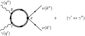
Figure 1: The Feynman diagram for the $\nu\nu\gamma\gamma$-interaction in magnetic field.

The general form for the matrix element corresponding to diagrams in Fig. 1 is the following

$${\cal S} = \frac{i4\pi\alpha G_{F}/\sqrt{2}}{\sqrt{2E^{\prime}V\,2E^{\prime\prime}V\,2\omega^{\prime}V\,2\omega^{\prime\prime}V}}\int d^{4}x\,d^{4}y\,d^{4}z\,Sp\{(j\gamma)(g_{V}-g_{A}\gamma_{5})S(x,y)\times$$ (6)

$$\times \ (\varepsilon^{\prime\prime}\gamma)S(y,z)(\varepsilon^{\prime}\gamma)S(z,x)\}e^{-i(kx-q^{\prime}z-q^{\prime\prime}y)}+(\varepsilon^{\prime},q^{\prime}\leftrightarrow\varepsilon^{\prime\prime},q^{\prime\prime}),$$

where $\alpha\simeq 1/137$ is the fine-structure constant; $q^{\prime}_{\alpha}=(\omega^{\prime},{\bf q^{\prime}}),\,q^{\prime\prime}_{\alpha}=(\omega^{\prime\prime},{\bf q^{\prime\prime}})$ are the four-momenta of the initial photons with polarisation vectors $\varepsilon^{\prime}_{\alpha},\varepsilon^{\prime\prime}_{\alpha}$ respectively; $k_{\alpha}$ is the neutrino antineutrino pair four-momentum. $S(x,y)$ is the electron propagator in the magnetic field which could be presented in the form

$$S(x,y) = e^{i\Phi(x,y)}\hat{S}(x-y),$$ (7)

$$\Phi(x,y) = -e\int\limits_{x}^{y}d\xi_{\mu}\left[A_{\mu}(\xi)+\frac{1}{2}F_{\mu\nu}(\xi-y)_{\mu}\right],$$ (8)

where $A_{\mu}$ and $F_{\mu\nu}$ are 4-potential and tensor of the uniform magnetic filed correspondingly. The translational invariant part $\hat{S}(x-y)$ has different representations. For our purpose it is convenient to take it in the following form

$$\hat{S}(X)=\hat{S}_{-}(X)+\hat{S}_{+}(X)+\hat{S}_{\mbox{\tiny$\bot$}}(X),$$ (9)

where

$$\hat{S}_{\pm}(X) = -\frac{i}{4\pi}\int\limits^{\infty}_{0}\frac{d\tau}{\rm tanh\tau}\,\int\frac{d^{2}p}{(2\pi)^{2}}[(p\gamma)_{\mbox{\tiny$\|$}}+m]\Pi_{\pm}(1\mp\rm tanh\tau)\times$$ (10)

$$\times \exp\left(-\frac{eB\,X_{\mbox{\tiny$\bot$}}^{2}}{4\,\rm tanh\tau}-\frac{\tau(m^{2}-p_{\mbox{\tiny$\|$}}^{2})}{eB}-i(pX)_{\mbox{\tiny$\|$}}\right),$$

$$\hat{S}_{\mbox{\tiny$\bot$}}(X) = -\frac{eB}{8\pi}\int\limits^{\infty}_{0}\frac{d\tau}{\rm tanh^{2}\tau}\,\int\frac{d^{2}p}{(2\pi)^{2}}(X\gamma)_{\mbox{\tiny$\bot$}}(1-\rm tanh^{2}\tau)\times$$ (11)

$$\times \exp\left(-\frac{eB\,X_{\mbox{\tiny$\bot$}}^{2}}{4\,\rm tanh\tau}-\frac{\tau(m^{2}-p_{\mbox{\tiny$\|$}}^{2})}{eB}-i(pX)_{\mbox{\tiny$\|$}}\right).$$

$$d^{2}p = dp_{0}dp_{3},\quad\Pi_{\pm}=\frac{1}{2}(1\pm i\gamma_{1}\gamma_{2}),\quad\Pi^{2}_{\pm}=\Pi_{\pm},\quad[\Pi_{\pm},(A\gamma)_{\mbox{\tiny$\|$}}]=0.$$

Here $\gamma_{\alpha}$ are the Dirac matrices in the standard representation, the four-vectors with the indices $\bot$ and $\parallel$ belong to the Euclidean (1, 2) subspace and the Minkowski (0, 3) subspace correspondingly, when the field $\bf B$ is directed along the third axis. Then for arbitrary 4-vectors $A_{\mu}$, $B_{\mu}$ one has

$$A_{\mbox{\tiny$\bot$}}^{\mu} = (0,A_{1},A_{2},0),\quad A_{\mbox{\tiny$\|$}}^{\mu}=(A_{0},0,0,A_{3}),$$

$$(AB)_{\mbox{\tiny$\bot$}} = (A\Lambda B)=A_{1}B_{1}+A_{2}B_{2},\quad(AB)_{\mbox{\tiny$\|$}}=(A\widetilde{\Lambda}B)=A_{0}B_{0}-A_{3}B_{3},$$

where the matrices $\Lambda_{\mu\nu}=(\varphi\varphi)_{\mu\nu}$,  $\widetilde{\Lambda}_{\mu\nu}=(\tilde{\varphi}\tilde{\varphi})_{\mu\nu}$ are constructed with the dimensionless tensor of the external magnetic field, $\varphi_{\mu\nu}=F_{\mu\nu}/B$, and the dual one, ${\tilde{\varphi}}_{\mu\nu}=\frac{1}{2}\varepsilon_{\mu\nu\rho\sigma}\varphi_{\rho\sigma}$. Matrices $\Lambda_{\mu\nu}$ and $\widetilde{\Lambda}_{\mu\nu}$ are connected by the relation $\widetilde{\Lambda}_{\mu\nu}-\Lambda_{\mu\nu}=g_{\mu\nu}=diag(1,-1,-1,-1)$, and play the role of the metric tensors in perpendicular ($\bot$) and parallel ($\parallel$) subspaces respectively.

In spite of the translational and gauge noninvariance of the phase $\Phi(x,y)$ in the propagator (7), the total phase of three propagators in the loop of Fig.1 is translational and gauge invariant

$$\Phi(x,y)+\Phi(y,z)+\Phi(z,x)=-\frac{e}{2}(z-x)_{\mu}F_{\mu\nu}(x-y)_{\nu}.$$

This fact allows one to define the amplitude of the process in the standard manner

$${\cal S}=\frac{i(2\pi)^{4}\delta^{4}(k-q^{\prime}-q^{\prime\prime})}{\sqrt{2E^{\prime}V\,2E^{\prime\prime}V\,2\omega^{\prime}V\,2\omega^{\prime\prime}V}}\,{\cal M},$$ (12)

where the amplitude ${\cal M}$ can be presented in the following form

$${\cal M}=\frac{G_{F}}{\sqrt{2}\ e}\,j_{\mu}\varepsilon^{\prime\prime}_{\nu}\varepsilon^{\prime}_{\rho}\{g_{V}\Pi^{V}_{\mu\nu\rho}-g_{A}\Pi^{A}_{\mu\nu\rho}\},$$ (13)

$$\Pi^{V}_{\mu\nu\rho} = e^{3}\int d^{4}X\,d^{4}Y\,Sp\{\gamma_{\mu}\hat{S}(X)\gamma_{\nu}\ \hat{S}(-X-Y)\gamma_{\rho}\hat{S}(Y)\}\times$$ (14)

$$\times e^{-ie\,(XFY)/2}\;e^{i(q^{\prime}X-q^{\prime\prime}Y)}+(\varepsilon^{\prime},q^{\prime}\leftrightarrow\varepsilon^{\prime\prime},q^{\prime\prime}),$$

$$\Pi^{A}_{\mu\nu\rho} = e^{3}\int d^{4}X\,d^{4}Y\,Sp\{\gamma_{\mu}\gamma_{5}\hat{S}(X)\gamma_{\nu}\ \hat{S}(-X-Y)\gamma_{\rho}\hat{S}(Y)\}\times$$ (15)

$$\times e^{-ie\,(XFY)/2}\;e^{i(q^{\prime}X-q^{\prime\prime}Y)}+(\varepsilon^{\prime},q^{\prime}\leftrightarrow\varepsilon^{\prime\prime},q^{\prime\prime}),$$

with $X=z-x,\,Y=x-y$.

In a general case substitution of the propagator (7) into the amplitude (13) leads to a very cumbersome expression in the form of the triple integral over the proper time. It is advantageous to use the asymptotic expression of the electron propagator for an analysis of the amplitude in strong magnetic field. This asymptotic could be derived from Eqs.(7)-(11) in the limit $eB/|m^{2}~{}-~{}p_{\mbox{\tiny$\|$}}^{2}~{}|~{}\gg~{}1$. In this case the parts $\hat{S}_{\pm},\,\hat{S}_{\mbox{\tiny$\bot$}}$ of the propagator take the form

$$\hat{S}_{-}(X)\simeq\frac{ieB}{2\pi}\exp(-\frac{eBX_{\mbox{\tiny$\bot$}}^{2}}{4})\int\frac{d^{2}p}{(2\pi)^{2}}\,\frac{(p\gamma)_{\mbox{\tiny$\|$}}+m}{p_{\mbox{\tiny$\|$}}^{2}-m^{2}}\Pi_{-}e^{-i(pX)_{\mbox{\tiny$\|$}}},$$ (16)

$$\hat{S}_{+}(X)\simeq-\frac{i}{4\pi}\,[i(\gamma\,\partial/\partial X)_{\mbox{\tiny$\|$}}+m]\,\delta_{\mbox{\tiny$\|$}}^{2}(X)\,\Pi_{+}\,\exp(\frac{eBX_{\mbox{\tiny$\bot$}}^{2}}{4})\,\Gamma(0,\frac{eBX_{\mbox{\tiny$\bot$}}^{2}}{2}),$$ (17)

$$\hat{S}_{\mbox{\tiny$\bot$}}(X)\simeq-\frac{1}{2\pi}\,\delta_{\mbox{\tiny$\|$}}^{2}(X)\,\frac{(X\gamma)_{\mbox{\tiny$\bot$}}}{X_{\mbox{\tiny$\bot$}}^{2}}\exp(-\frac{eBX_{\mbox{\tiny$\bot$}}^{2}}{4}),$$ (18)

where $\Gamma(a,z)$ is the incomplete gamma function $\Gamma(a,z)=\int\limits^{\infty}_{z}t^{a-1}e^{-t}dt.$

By using, (16)-(18) the amplitude ${\cal M}$ can be presented as a sum of the ten independent parts which can conditionally be divided into four groups: 1) $\hat{S}_{\pm}\hat{S}_{\pm}\hat{S}_{\pm}$; 2) $\hat{S}_{\pm}\hat{S}_{\pm}\hat{S}_{\mbox{\tiny$\bot$}}$; 3) $\hat{S}_{\pm}\hat{S}_{\mbox{\tiny$\bot$}}\hat{S}_{\mbox{\tiny$\bot$}}$; 4) $\hat{S}_{\mbox{\tiny$\bot$}}\hat{S}_{\mbox{\tiny$\bot$}}\hat{S}_{\mbox{\tiny$\bot$}}$. Analysing these combinations one could expect that the leading on field strength part of the amplitude, namely $\sim eB$, arises from the combination $\hat{S}_{-}\hat{S}_{-}\hat{S}_{-}$. Really, substitution of $\hat{S}_{-}$ in amplitude (13) gives $(eB)^{3}$ in numerator, while integration over transverse coordinates $X_{\mbox{\tiny$\bot$}}$ leads to the factor $(eB)^{2}$ in denominator. Then expending the amplitude in powers of inverse magnetic field strength B we obtain the linear on field dependence. However, it is easy to see that two parts of the amplitude (13) with photons exchange $(\varepsilon^{\prime},q^{\prime}\leftrightarrow\varepsilon^{\prime\prime},q^{\prime\prime})$ cancel each other exactly in this limit. Hence the amplitude of the process $\gamma\gamma\to\nu\bar{\nu}$ doesn’t depend on B in the strong magnetic field.

The analysis shows that the independent on field contribution to the amplitude is given by the combinations $\hat{S}_{-}\hat{S}_{-}\hat{S}_{+},\,\hat{S}_{-}\hat{S}_{-}\hat{S}_{\mbox{\tiny$\bot$}}$ and $\hat{S}_{-}\hat{S}_{\mbox{\tiny$\bot$}}\hat{S}_{\mbox{\tiny$\bot$}}$ with all interchanges. One more contribution comes from the expansion of the $\hat{S}_{-}\hat{S}_{-}\hat{S}_{-}$ combination in the powers of inverse magnetic field strength $B$. Then substituting (16)-(18) into (13) we obtain the following result for the amplitude

$${\cal M}\simeq\frac{G_{F}}{\sqrt{2}\ e}\,j_{\mu}\varepsilon^{\prime\prime}_{\nu}\varepsilon^{\prime}_{\rho}\{g_{V}\Pi^{V}_{\mu\nu\rho}-g_{A}\Pi^{A}_{\mu\nu\rho}\},$$ (19)

$$\Pi^{V}_{\mu\nu\rho} = -\frac{ie^{3}}{2\pi^{2}}\{(q^{\prime}\varphi q^{\prime\prime})\,\pi_{\mu\nu\rho}+(q^{\prime}I^{\prime\prime})_{\nu}\,\varphi_{\rho\mu}+\frac{1}{2}((q^{\prime\prime}-q^{\prime})I)_{\mu}\,\varphi_{\nu\rho}$$ (20)

$$+ (q^{\prime\prime}I^{\prime})_{\rho}\,\varphi_{\nu\mu}-I^{\prime\prime}_{\nu\rho}\,(q^{\prime}\varphi)_{\mu}+I^{\prime\prime}_{\mu\nu}\,(q\varphi)_{\rho}+I^{\prime}_{\mu\rho}\,(q\varphi)_{\nu}$$

$$- I^{\prime}_{\nu\rho}\,(q^{\prime\prime}\varphi)_{\mu}-I_{\mu\nu}\,(q^{\prime\prime}\varphi)_{\rho}-I_{\mu\rho}\,(q^{\prime}\varphi)_{\nu}\},$$

$$\Pi^{A}_{\mu\nu\rho} = -\frac{ie^{3}}{2\pi^{2}}\{(q^{\prime}\varphi q^{\prime\prime})\,\tilde{\varphi}_{\mu\sigma}\pi_{\sigma\nu\rho}+(q^{\prime}\tilde{\varphi}I^{\prime\prime})_{\nu}\,\varphi_{\rho\mu}-\frac{1}{2}((q^{\prime\prime}-q^{\prime})I\tilde{\varphi})_{\mu}\,\varphi_{\nu\rho}$$ (21)

$$+ (q^{\prime\prime}\tilde{\varphi}I^{\prime})_{\rho}\,\varphi_{\nu\mu}-(\tilde{\varphi}I^{\prime\prime})_{\rho\nu}\,(q^{\prime}\varphi)_{\mu}+(\tilde{\varphi}I^{\prime\prime})_{\mu\nu}\,(q\varphi)_{\rho}+(\tilde{\varphi}I^{\prime})_{\mu\rho}\,(q\varphi)_{\nu}$$

$$- (\tilde{\varphi}I^{\prime})_{\nu\rho}\,(q^{\prime\prime}\varphi)_{\mu}-(\tilde{\varphi}I)_{\mu\nu}\,(q^{\prime\prime}\varphi)_{\rho}-(\tilde{\varphi}I)_{\mu\rho}\,(q^{\prime}\varphi)_{\nu}\}.$$

It is remarkable that the amplitude ${\cal M}$ depends only on two types of integrals, $I_{\mu\nu}$ and $\pi_{\mu\nu\rho}$

$$I_{\mu\nu} \equiv I_{\mu\nu}(q)=-i\pi\int\frac{d^{2}p}{(2\pi)^{2}}\,\mathrm{Sp}\{\gamma_{\mu}S_{\mbox{\tiny$\|$}}(p-q)\gamma_{\nu}S_{\mbox{\tiny$\|$}}(p)\},$$ (22)

$$\pi_{\mu\nu\rho} = -i\pi\int\frac{d^{2}p}{(2\pi)^{2}}\,\mathrm{Sp}\{\gamma_{\mu}S_{\mbox{\tiny$\|$}}(p-q^{\prime\prime})\gamma_{\nu}S_{\mbox{\tiny$\|$}}(p)\gamma_{\rho}S_{\mbox{\tiny$\|$}}(p+q^{\prime})\},$$ (23)

with

$$S_{\mbox{\tiny$\|$}}(p)=\frac{(p\gamma)_{\mbox{\tiny$\|$}}+m}{p_{\mbox{\tiny$\|$}}^{2}-m^{2}}\,\Pi_{-}.$$

Both types of integrals (22) and (23) can be presented in terms of analytical functions. The integral $I_{\mu\nu}$ can be written as:

$$I_{\mu\nu}(q)=\bigg{(}\tilde{\Lambda}_{\mu\nu}-\frac{q_{\mbox{\tiny$\|$}\mu}\,q_{\mbox{\tiny$\|$}\nu}}{q^{2}_{\mbox{\tiny$\|$}}}\bigg{)}\,H\!\!\left(\frac{4m_{e}^{2}}{q_{\mbox{\tiny$\|$}}^{2}}\right),$$

where

$$H(z)=\frac{z}{\sqrt{z-1}}\arctan\frac{1}{\sqrt{z-1}}-1,\ z>1,$$

$$H(z)=-\frac{1}{2}\left(\frac{z}{\sqrt{1-z}}\ln\frac{1+\sqrt{1-z}}{1-\sqrt{1-z}}+2-i\pi\frac{z}{\sqrt{1-z}}\right),\ z<1.$$

The expression for $\pi_{\mu\nu\rho}$ can be presented in the following form:

$$\pi_{\mu\nu\rho}=\frac{1}{q^{2}_{\mbox{\tiny$\|$}}q^{\prime 2}_{\mbox{\tiny$\|$}}q^{\prime\prime 2}_{\mbox{\tiny$\|$}}}\Big{[}(q^{\prime}\tilde{\varphi}q^{\prime\prime})\big{\{}(\tilde{\varphi}q)_{\mu}(\tilde{\varphi}q^{\prime\prime})_{\nu}(\tilde{\varphi}q^{\prime})_{\rho}\pi_{\mbox{\tiny$\bot$}}$$

$$+(\tilde{\varphi}q)_{\mu}(\widetilde{\Lambda}q^{\prime\prime})_{\nu}(\widetilde{\Lambda}q^{\prime})_{\rho}H-(\widetilde{\Lambda}q)_{\mu}(\tilde{\varphi}q^{\prime\prime})_{\nu}(\widetilde{\Lambda}q^{\prime})_{\rho}H^{\prime\prime}-(\widetilde{\Lambda}q)_{\mu}(\widetilde{\Lambda}q^{\prime\prime})_{\nu}(\tilde{\varphi}q^{\prime})_{\rho}H^{\prime}\big{\}}$$

$$+(q^{\prime}q^{\prime\prime})_{\mbox{\tiny$\|$}}(\widetilde{\Lambda}q)_{\mu}(\tilde{\varphi}q^{\prime\prime})_{\nu}(\tilde{\varphi}q^{\prime})_{\rho}(H^{\prime\prime}-H^{\prime})+(qq^{\prime\prime})_{\mbox{\tiny$\|$}}(\tilde{\varphi}q)_{\mu}(\tilde{\varphi}q^{\prime\prime})_{\nu}(\widetilde{\Lambda}q^{\prime})_{\rho}(H-H^{\prime\prime})$$

$$+(qq^{\prime})_{\mbox{\tiny$\|$}}(\tilde{\varphi}q)_{\mu}(\widetilde{\Lambda}q^{\prime\prime})_{\nu}(\tilde{\varphi}q^{\prime})_{\rho}(H^{\prime}-H)\Big{]},$$ (24)

$$\!\!\!\!\!\!\!\!\!\!\!\!\!\!\!\!\!\!\!\!\!\!\!\!\!\pi_{\mbox{\tiny$\bot$}} = H^{\prime}+H^{\prime\prime}+H$$ (25)

$$+ 2\frac{q^{2}_{\mbox{\tiny$\|$}}q^{\prime 2}_{\mbox{\tiny$\|$}}q^{\prime\prime 2}_{\mbox{\tiny$\|$}}-2m_{e}^{2}[q^{2}_{\mbox{\tiny$\|$}}(q^{\prime}q^{\prime\prime})_{\mbox{\tiny$\|$}}H-q^{\prime 2}_{\mbox{\tiny$\|$}}(qq^{\prime\prime})_{\mbox{\tiny$\|$}}H^{\prime}-q^{\prime\prime 2}_{\mbox{\tiny$\|$}}(qq^{\prime})_{\mbox{\tiny$\|$}}H^{\prime\prime}]}{q^{2}_{\mbox{\tiny$\|$}}q^{\prime 2}_{\mbox{\tiny$\|$}}q^{\prime\prime 2}_{\mbox{\tiny$\|$}}-4m_{e}^{2}[q^{\prime 2}_{\mbox{\tiny$\|$}}q^{\prime\prime 2}_{\mbox{\tiny$\|$}}-(q^{\prime}q^{\prime\prime})^{2}_{\mbox{\tiny$\|$}}]}.$$

where, e.g. $H^{\prime}\equiv H(4m_{e}^{2}/q^{\prime 2}_{\mbox{\tiny$\|$}})$. The result (19) can be also treated as an effective Lagrangian of photon-neutrino interaction in the momentum representation. Moreover it can be used to obtain the effective Lagrangians of axion-two photon ($a\gamma\gamma$) and three photon ($\gamma\gamma\gamma$) interactions by making the substitutions

$${\cal M}_{a\gamma\gamma}={\cal M}(g_{V}=0,\ g_{A}\frac{G_{F}}{\sqrt{2}}j_{\mu}\to\frac{ig_{ae}}{2m_{e}}\,q_{\mu})$$

and

$${\cal M}_{\gamma\gamma\gamma}={\cal M}(g_{A}=0,\ g_{V}\frac{G_{F}}{\sqrt{2}e}j_{\mu}\to\varepsilon_{\mu})$$

correspondingly. Here $g_{ae}$ is the axion-electron coupling.

Note also that the amplitude (19) in the low energy limit, $\omega\ll m_{e}$, with $g_{V}=g_{A}=1$ coincides with the amplitude obtained in [21].

3 Contribution of the process $\gamma\gamma\to\nu\bar{\nu}$ into the neutrino emissivity of the photon gas

To illustrate a possible application of the result obtained let us estimate the contribution of the process $\gamma\gamma\to\nu\bar{\nu}$ into the neutrino emissivity of the photon gas in strong magnetic field. It is convenient now to turn from the general amplitude (19) to the partial amplitudes corresponding to definite photon modes with polarisation vectors $\varepsilon^{(\mbox{\tiny$\|$})}_{\alpha}=(\varphi q)_{\alpha}/\sqrt{q_{\mbox{\tiny$\bot$}}^{2}},\,\varepsilon^{(\mbox{\tiny$\bot$})}_{\alpha}=(\tilde{\varphi}q)_{\alpha}/\sqrt{q_{\mbox{\tiny$\|$}}^{2}}$ (in Adler’s notation [22]). These amplitudes can be written as

$${\cal M}_{\mbox{\tiny$\|$}\mbox{\tiny$\|$}}=i\frac{2\alpha}{\pi}\,\frac{G_{F}}{\sqrt{2}}\,\frac{(q^{\prime}\varphi q^{\prime\prime})(q^{\prime}\tilde{\varphi}q^{\prime\prime})}{q^{2}_{\mbox{\tiny$\|$}}\sqrt{q^{\prime\prime 2}_{\mbox{\tiny$\bot$}}q^{\prime 2}_{\mbox{\tiny$\bot$}}}}\;[g_{V}(j\tilde{\varphi}q)-g_{A}(jq)_{\mbox{\tiny$\|$}}]\;H,$$ (26)

$${\cal M}_{\mbox{\tiny$\|$}\mbox{\tiny$\bot$}}=-i\frac{2\alpha}{\pi}\,\frac{G_{F}}{\sqrt{2}}\,\frac{1}{\sqrt{q^{\prime\prime 2}_{\mbox{\tiny$\bot$}}q^{\prime 2}_{\mbox{\tiny$\|$}}}}\;$$

$$\times\Bigg{\{}g_{V}\Bigg{(}[(j\tilde{\varphi}q^{\prime})(qq^{\prime\prime})_{\mbox{\tiny$\bot$}}+(jq^{\prime\prime})_{\mbox{\tiny$\bot$}}(q^{\prime}\tilde{\varphi}q^{\prime\prime})]H^{\prime}-\frac{(j\tilde{\varphi}q)(qq^{\prime})_{\mbox{\tiny$\|$}}(q^{\prime}q^{\prime\prime})_{\mbox{\tiny$\bot$}}}{q_{\mbox{\tiny$\|$}}^{2}}H\Bigg{)}$$

$$-g_{A}\bigg{(}[(jq^{\prime})_{\mbox{\tiny$\|$}}(qq^{\prime\prime})_{\mbox{\tiny$\bot$}}-(jq^{\prime\prime})_{\mbox{\tiny$\bot$}}(q^{\prime}q^{\prime\prime})_{\mbox{\tiny$\|$}}]H^{\prime}-\frac{(jq)_{\mbox{\tiny$\|$}}(qq^{\prime})_{\mbox{\tiny$\|$}}(q^{\prime}q^{\prime\prime})_{\mbox{\tiny$\bot$}}}{q_{\mbox{\tiny$\|$}}^{2}}H\bigg{)}\Bigg{\}},$$ (27)

$${\cal M}_{\mbox{\tiny$\bot$}\mbox{\tiny$\bot$}}=-i\frac{2\alpha}{\pi}\,\frac{G_{F}}{\sqrt{2}}\,\frac{1}{\sqrt{q^{\prime 2}_{\mbox{\tiny$\|$}}q^{\prime\prime 2}_{\mbox{\tiny$\|$}}}}\;\Bigg{\{}\frac{(q^{\prime}\varphi q^{\prime\prime})}{q^{2}_{\mbox{\tiny$\|$}}}\Big{(}(q^{\prime}\tilde{\varphi}q^{\prime\prime})[g_{V}(j\tilde{\varphi}q)-g_{A}(jq)_{\mbox{\tiny$\|$}}]\pi_{\mbox{\tiny$\bot$}}$$

$$+(q^{\prime}q^{\prime\prime})_{\mbox{\tiny$\|$}}[g_{V}(jq)_{\mbox{\tiny$\|$}}-g_{A}(j\tilde{\varphi}q)](H^{\prime\prime}-H^{\prime})\Big{)}-(j\varphi q^{\prime})H^{\prime\prime}[g_{V}(q^{\prime}q^{\prime\prime})_{\mbox{\tiny$\|$}}-g_{A}(q^{\prime}\tilde{\varphi}q^{\prime\prime})]$$

$$-(j\varphi q^{\prime\prime})H^{\prime}[g_{V}(q^{\prime}q^{\prime\prime})_{\mbox{\tiny$\|$}}+g_{A}(q^{\prime}\tilde{\varphi}q^{\prime\prime})]\Bigg{\}}$$ (28)

Then the neutrino emissivity (energy carried out by neutrinos from unit volume per unit time) can be defined as

$$Q_{\gamma\gamma\to\nu\bar{\nu}}^{B}=Q_{\mbox{\tiny$\|$}\mbox{\tiny$\|$}}+Q_{\mbox{\tiny$\bot$}\mbox{\tiny$\|$}}+Q_{\mbox{\tiny$\bot$}\mbox{\tiny$\bot$}},$$ (29)

$$Q_{\lambda^{\prime}\lambda^{\prime\prime}} = (2\pi)^{4}g_{\lambda^{\prime}\lambda^{\prime\prime}}\sum\limits_{i}\int|{\cal M}_{\lambda^{\prime}\lambda^{\prime\prime}}|^{2}Z_{\lambda^{\prime}}Z_{\lambda^{\prime\prime}}(E_{i}^{\prime}+E_{i}^{\prime\prime})\,\delta^{4}(q^{\prime}+q^{\prime\prime}-k^{\prime}-k^{\prime\prime})$$ (30)

$$\times \frac{d^{3}q^{\prime}}{(2\pi)^{3}2\omega^{\prime}}\,f(\omega^{\prime})\,\frac{d^{3}q^{\prime\prime}}{(2\pi)^{3}\,2\,\omega^{\prime\prime}}\,f(\omega^{\prime\prime})\,\frac{d^{3}k^{\prime}}{(2\pi)^{3}\,2\,E_{i}^{\prime}}\,\frac{d^{3}k^{\prime\prime}}{(2\pi)^{3}\,2\,E_{i}^{\prime\prime}}.$$

Here $E_{i}^{\prime},E_{i}^{\prime\prime}$ are the energies of the neutrino and antineutrino of definite types $i=\nu_{e},\nu_{\mu},\nu_{\tau}$; $\omega^{\prime},\omega^{\prime\prime}$ are the energies of the initial photons; $f(\omega)=[\exp(\omega/T)-1]^{-1}$ is the photon distribution function at the temperature $T$; the factor $g_{\lambda^{\prime}\lambda^{\prime\prime}}=1-\frac{1}{2}\delta_{\lambda^{\prime}\lambda^{\prime\prime}}$ is inserted to account for the possible identity of the photons in the initial state. We would like to note that the integration over the phase space of initial photons in (30) has to be performed taking account for nontrivial photon dispersion law in the presence of strong magnetic field. Moreover, it is necessary to take into consideration the large radiative corrections in strong magnetic field which are reduced to the wave-function renormalization factors $Z_{\lambda^{\prime}}$ and $Z_{\lambda^{\prime\prime}}$ in Eq. (30). In the case of low temperature, $T\ll m_{e}$ the dispersion law of the photon with polarization vector $\varepsilon^{(\mbox{\tiny$\bot$})}_{\alpha}$ and corresponding wave-function renormalization factor $Z_{\mbox{\tiny$\bot$}}$ could be presented in the following form

$$\omega^{2}=\frac{q_{\mbox{\tiny$\bot$}}^{2}}{(1+\xi)}+q_{3}^{2},\qquad Z_{\mbox{\tiny$\bot$}}\simeq\frac{1}{1+\xi},$$ (31)

where $\xi=\frac{\alpha}{3\pi}\,\frac{B}{B_{e}}$ is factor characterising magnetic field influence. The photon with polarization vector $\varepsilon^{(\mbox{\tiny$\|$})}_{\alpha}$ has almost vacuum dispersion law and wave-function renormalization factor in this limit, $q^{2}\simeq 0,\,\,Z_{\mbox{\tiny$\|$}}\simeq 1$. It is useful also to present here the element of the momentum space

$$d^{3}q=(1+\xi)\,\omega^{2}\,d\omega\,d\varphi\,dy,\qquad y=\cos\theta\sqrt{1+\xi}/\sqrt{1+\xi\cos^{2}\theta},$$ (32)

where $\theta,\phi$ are the polar and the azimutal angles. All of these facts lead to the rather complicated dependence of $Q_{\gamma\gamma\to\nu\bar{\nu}}^{B}$ on magnetic field strength despite the amplitude (19) does not contain this dependence. In the case of the arbitrary parameter $\xi$ the value of the contribution into neutrino emissivity of the photon gas can be found only numerically, but when the strength of magnetic field is not too large, $eB\ll m_{e}^{2}/\alpha$, one can obtain the analitical expressions for $Q_{\lambda^{\prime}\lambda^{\prime\prime}}$:

$$Q_{\mbox{\tiny$\|$}\mbox{\tiny$\|$}} = \frac{8\,\alpha^{2}G_{F}^{2}}{8505\,\pi^{3}\,m_{e}^{4}}\,\,T^{13}\,\bigg{[}{\bar{g}}_{V}^{2}\pi^{2}\left(7\pi^{2}\zeta(5)+330\,\zeta(7)\right)$$ (33)

$$+ {\bar{g}}_{A}^{2}\left(9\pi^{4}\zeta(5)+70\pi^{2}\zeta(7)+420\,\zeta(9)\right)\bigg{]}$$

$$\simeq 8.5\cdot 10^{7}\,T_{9}^{13}\,\frac{\mbox{erg}}{\mbox{s}\cdot\mbox{cm}^{3}}\,,$$

$$Q_{\mbox{\tiny$\|$}\mbox{\tiny$\perp$}} = \frac{32\,\alpha^{2}G_{F}^{2}}{127575\,\pi^{3}\,m_{e}^{4}}\,T^{13}\,\bigg{[}{\bar{g}}_{V}^{2}24\pi^{2}\left(14\pi^{2}\zeta(5)+285\,\zeta(7)\right)$$ (34)

$$+ {\bar{g}}_{A}^{2}\left((309\pi^{2}+20)\pi^{2}\zeta(5)+(1410\pi^{2}+315)\zeta(7)+38430\,\zeta(9)\right)\bigg{]}$$

$$\simeq 6.9\cdot 10^{8}\,T_{9}^{13}\,\frac{\mbox{erg}}{\mbox{s}\cdot\mbox{cm}^{3}}\,,$$

$$Q_{\mbox{\tiny$\perp$}\mbox{\tiny$\perp$}} = \frac{8\,\alpha^{2}G_{F}^{2}}{127575\,\pi^{3}\,m_{e}^{4}}\,T^{13}\,\bigg{[}{\bar{g}}_{V}^{2}\pi^{2}\left((609\pi^{2}-50)\zeta(5)+10110\,\zeta(7)\right)$$ (35)

$$+ {\bar{g}}_{A}^{2}\left((879\,\pi^{2}+50)\pi^{2}\zeta(5)+5490\pi^{2}\zeta(7)+56700\,\zeta(9)\right)\bigg{]}$$

$$\simeq 3.3\cdot 10^{8}\,T_{9}^{13}\,\frac{\mbox{erg}}{\mbox{s}\cdot\mbox{cm}^{3}}\,.$$

Here $T_{9}$ is the temperature in units of $10^{9}K\simeq 0.17m_{e}$, the effective constants ${\bar{g}}_{V}^{2}\simeq 0.93,\,{\bar{g}}_{A}^{2}\simeq 0.75$ are summarized over all channels of the neutrino production, $\nu_{e},\nu_{\mu},\nu_{\tau}$. The total neutrino emissivity in this case is

$$Q_{\gamma\gamma\to\nu\bar{\nu}}^{LT}\simeq 1.1\cdot 10^{9}\,T_{9}^{13}\,\frac{\mbox{erg}}{\mbox{s}\cdot\mbox{cm}^{3}}\,.$$ (36)

We also have made the numerical calculation of the neutrino emissivity caused by the process $\gamma\gamma\to\nu\bar{\nu}$. In the low temperature limit $T\ll m_{e}$ our result is represented in Fig. 2 where the emissivity $Q_{\gamma\gamma\to\nu\bar{\nu}}^{B}$ is depicted as a function of the parameter $\xi$.

Figure 2: The low temperature, $T\ll m_{e}$, neutrino emissivity $Q_{\gamma\gamma\to\nu\bar{\nu}}^{B}$ dependence on the parameter $\xi=\frac{\alpha}{3\pi}\,\frac{B}{B_{e}}$ for different polarisation configurations of the initial photons; $Q_{0}=10^{8}T_{9}^{13}\,\mbox{\small erg}/(\mbox{\small s}\cdot\mbox{\small cm}^{3})$. Short-dashed, dash-dotted and long-dashed curves correspond to $Q_{\mbox{\tiny$\|$}\mbox{\tiny$\|$}},Q_{\mbox{\tiny$\bot$}\mbox{\tiny$\|$}},Q_{\mbox{\tiny$\bot$}\mbox{\tiny$\bot$}}$ respectively. Solid line depicts the total neutrino emissivity.

The result presented by formular (36) and in Fig. 2 should be compared with the contributions into the neutrino emissivity of the process $\gamma\gamma\to\nu\bar{\nu}$ caused by the another mechanisms. For instance, the emissivity due to the finite neutrino mass is [7]

$$Q_{\gamma\gamma\to\nu\bar{\nu}}^{m_{\nu}}\simeq 1.4\cdot 10^{-4}\,T_{9}^{11}\,\frac{\mbox{erg}}{\mbox{s}\cdot\mbox{cm}^{3}}\,\left(\frac{m_{\nu}}{1\,\mbox{eV}}\right)^{2}.$$ (37)

On the other hand, in the case of non-locality of the weak interaction, investigated in Ref. [10], one can estimate the emissivity, which is suppressed by the factor $(m_{e}/m_{W})^{4}$:

$$Q_{\gamma\gamma\to\nu\bar{\nu}}^{NL}\simeq 9.9\cdot 10^{-10}\,T_{9}^{13}\,\frac{\mbox{erg}}{\mbox{s}\cdot\mbox{cm}^{3}}\,.$$ (38)

It’s obvious that the field-induced mechanism of the reaction $\gamma\gamma\to\nu\bar{\nu}$ strongly dominates all the other mechanisms.

It is interesting also to compare our result with the previous calculations of the neutrino emissivity due the process $\gamma\gamma\to\nu\bar{\nu}$ in the weak and strong magnetic fields. Taking into account the remark by authors of [20] one could obtain from [16] the following estimation for the neutrino emissivity $Q_{\gamma\gamma\to\nu\bar{\nu}}^{B}$ in the weak magnetic field limit, $B\ll B_{e}$:

$$Q_{\gamma\gamma\to\nu\bar{\nu}}^{B}\simeq 0.3\cdot 10^{9}\,T_{9}^{13}\left(\frac{B}{B_{e}}\right)^{2}\frac{\mbox{erg}}{\mbox{s}\cdot\mbox{cm}^{3}}.$$ (39)

It is evident that neutrino emissivity is substantially enhanced in strong magnetic field in comparison with its counterpart in the weak magnetic field case.

In the limit $B\gg B_{e}$ the contribution of the process $\gamma\gamma\to\nu\bar{\nu}$ into the neutrino emissivity was previously studied in [21], from which the following estimation could be obtained:

$$Q_{\gamma\gamma\to\nu\bar{\nu}}^{B}\simeq 0.7\cdot 10^{8}\,T_{9}^{13}\frac{\mbox{erg}}{\mbox{s}\cdot\mbox{cm}^{3}}.$$ (40)

This result doesn’t depend on the magnetic field strength $B$ and it is at least ten times less than our result presented in Fig. 2. In our opinion, the authors [21] wrongfully didn’t take into account photon dispersion and wave-function renormalisation in strong magnetic field.

Let us note that in the presence of the magnetic field one more contribution into neutrino emissivity due to the process $\gamma\to\gamma\nu\bar{\nu}$ is possible. We would like to emphasize that it is the nontrivial dispersion law of a photon in the magnetic field that makes this reaction to be kinematically allowed. To our knowledge the process $\gamma\to\gamma\nu\bar{\nu}$ has not been studied so far. Therefore it is interesting to compare the contributions into the neutrino emissivity from the $\gamma\gamma\to\nu\bar{\nu}$ and $\gamma\to\gamma\nu\bar{\nu}$ channels.

To obtain the emissivity by the process $\gamma\to\gamma\nu\bar{\nu}$ one needs to make the replacements $f(\omega)\to(1+f(\omega))$ and $q\to-q$ for one of the photons in (30). The analysis of the process kinematics shows that only one transition, $\gamma_{\mbox{\tiny$\|$}}\to\gamma_{\mbox{\tiny$\bot$}}\nu\bar{\nu}$, gives the contribution into neutrino emissivity. The dependence of the neutrino emissivity due to the process $\gamma\to\gamma\nu\bar{\nu}$ on the magnetic field strength is depicted in Fig.3.

Figure 3: The low temperature, $T\ll m_{e}$, neutrino emissivity $Q_{\gamma\to\gamma\nu\bar{\nu}}^{B}$ dependence on the parameter $\xi$.

As is seen from both figures the contribution of the process $\gamma\to\gamma\nu\bar{\nu}$ into the neutrino emissivity turns out to be small in comparison with analogous contribution due to the reaction $\gamma\gamma\to\nu\bar{\nu}$ in the case of not too strong magnetic field, $B\ll 10^{5}B_{e}$.

In the high temperature limit, $T\gg m_{e}$, the main contribution into neutrino emissivity arises from the photons with parallel momenta squared are in the region $m_{e}^{2}\ll q_{\mbox{\tiny$\|$}}^{2}\ll eB$. In this case one can use vacuum dispersion law for both photon modes. We obtain the following estimation for neutrino emissivity in this limit:

$$Q_{\gamma\gamma\to\nu\bar{\nu}}^{HT}\simeq 2.7\cdot 10^{18}\left(\frac{T}{m_{e}}\right)^{9}\frac{\mbox{erg}}{\mbox{s}\cdot\mbox{cm}^{3}}\,.$$ (41)

Let us compare this result with contribution into neutrino emissivity from process $\gamma\to\nu\bar{\nu}$. In strong magnetic field this reaction was studied in [23]. It was shown that the process $\gamma\to\nu\bar{\nu}$ is kinematically allowed in the region $q^{2}_{\mbox{\tiny$\|$}}>4m^{2}$. This lad to the suppression of the process in the low temperature limit by factor $q_{\mbox{\tiny$\|$}}^{2}\simeq 4m_{e}^{2}$. In high temperature limit authors note that the main contribution into neutrino emissivity is defined by the vicinity of the point $q^{2}_{\mbox{\tiny$\|$}}=4m_{e}^{2}$. However, the detailed analysis shows that the main contribution arises from the region $m_{e}^{2}\ll q_{\mbox{\tiny$\|$}}^{2}\ll\beta$. In this case the estimation of the neutrino emissivity coincides with the formula obtained by authors in the limit $T^{2}\gg eB,m_{e}^{2}$:

$$Q_{\gamma\to\nu\bar{\nu}}^{HT}\simeq 0.40\cdot 10^{18}\left(\frac{T}{m_{e}}\right)^{5}\left(\frac{B}{B_{e}}\right)^{2}\frac{\mbox{erg}}{\mbox{s}\cdot\mbox{cm}^{3}}\,.$$ (42)

Then the ration of the emissivities (41) and (42) is

$$R=\frac{Q_{\gamma\to\nu\bar{\nu}}^{HT}}{Q_{\gamma\gamma\to\nu\bar{\nu}}^{HT}}\simeq 0.15\left(\frac{B}{T^{2}}\right)^{2}.$$ (43)

It is seen that the contribution into neutrino emissivity of the process $\gamma\to\nu\bar{\nu}$ is always larger then $\gamma\gamma\to\nu\bar{\nu}$ reaction contribution, because $B\gg T^{2}$ in strong magnetic field limit. For example, $R\simeq 5.86$ for $T=2$ MeV and $B=100B_{e}$. Nevertheless, we can see that these quantities have the comparable values.

In summary, we have investigated the two-photon two-neutrino processes in the presence of strong magnetic field. The amplitude of the reaction $\gamma\gamma\to\nu\bar{\nu}$ is obtained in a general case when the photons are not assumed to be on the mass shell. Therefore it can be treated as an effective Lagrangian of photon-neutrino interaction. We have also calculated the contribution into the neutrino emissivity due to the reactions $\gamma\gamma\to\nu\bar{\nu}$ and $\gamma\to\gamma\nu\bar{\nu}$ taking into account the photon dispersion and wave function renormalisation in strong magnetic field. We stress that in spite of the independence of the amplitude on the magnetic field strength $B$, the emissivity essentially depends on $B$. The comparison of our results with the other inducing mechanisms of the reaction $\gamma\gamma\to\nu\bar{\nu}$ shows that strong magnetic field catalyses this process. Moreover it seems that the processes under consideration are the most dominating photon-neutrino reactions.

Acknowledgements

M.C. expresses his deep gratitude to the organizers of the XXXI ITEP Winter School of Physics for warm hospitality.

This work was supported in part by the Russian Foundation for Basic Research under the Grant N 01-02-17334, by the Ministry of Education of Russian Federation under the Grant No. E02-11.0-48 and by Ministry of Industry, Science and Technologies of Russian Federation under the Grant No. NSh-1916.2003.2.

References

• [1] B. Pontecorvo, Zh. Eksper. Teor. Fiz. 9, 1615 (1959) [Sov. Phys. JETP 9, 1148 (1959)].
• [2] H.-E. Chiu, P. Morrison, Phys. Rev. Lett. 5, 573 (1960).
• [3] M. Gell-Mann, Phys. Rev. Lett. 6, 70 (1961).
• [4] L. D. Landau, Sov. Phys. Doklady 60, 207 (1948).
• [5] C. N. Yang, Phys. Rev. 77, 242 (1950).
• [6] R. J. Crewther, J. Finjord, P. Minkowski, Nucl. Phys. B 207, 269 (1982).
• [7] S. Dodelson, G. Feinberg, Phys. Rev. D 43, 913 (1991).
• [8] M. J. Levine, Nuovo Cim. 48, 67 (1967).
• [9] D. A. Dicus, Phys. Rev. D 6, 941 (1972).
• [10] D. A. Dicus, W. W. Repko, Phys. Rev. D 48, 5106 (1993).
• [11] V. K. Cung, M. Yoshimura, Nuovo Cim. A 29, 557 (1975).
• [12] A. V. Kuznetsov, N. V. Mikheev, Phys. Lett. B 299, 367 (1993).
• [13] G.S. Bisnovatyi-Kogan and S.G. Moiseenko, Astron. Zh. 69, 563 (1992) [Sov. Astron. 36, 285 (1992) ]; G.S. Bisnovatyi-Kogan, Astron. Astrophys. Transactions 3, 287 (1993); R.C. Duncan and C. Thompson, Astrophys.J. 392, L9 (1992); C. Thompson and R.C. Duncan, Mon.Not.R.Astron.Soc. 275, 255 (1995).
• [14] C. Kouveliotou et al, Nature, 393, 235 (1998); C. Kouveliotou et al, Astrophys.J. 510, L115 (1999); Kouveliotou, C. et al., Astrophys.J. 2001. V.558. P.L47; A. I. Ibrahim, S. Safi-Harb, J. H. Swank, W. Parke, S. Zane and R. Turolla, Astrophys. J. Lett. 574 (2002) L51; A. I. Ibrahim, J. H. Swank and W. Parke, Astrophys. J.  584 (2003) L17
• [15] Gvozdev A.A., Mikheev N.V., Vassilevskaya L.A. Phys. Rev. D54, N 9, 5674 (1996)
• [16] R. Shaisultanov, Phys. Rev. Lett. 80, 1586 (1998).
• [17] D. A. Dicus, W. W. Repko, Phys. Rev. Lett. 79, 569 (1997).
• [18] T. K. Chyi et al., Phys. Lett. B 466, 274 (1999).
• [19] T. K. Chyi et al., Phys. Rev. D 62, 105014 (2000).
• [20] D. A. Dicus, W. W. Repko, Phys.Lett. B 482, 141 (2000).
• [21] Yu. M. Loskutov and V. V. Skobelev, Vestn. Mosk. Univ. Fiz. Astron. 22, 10 (1981)
• [22] S.L. Adler, Ann. Phys. N.Y. 67, 599 (1971).
• [23] A.V. Kuznetsov, N.V. Mikheev, L.A. Vassilevskaya Phys.Lett. B 427, 105 (1998)