MCTP-03-39

SHEP-03/25

FERMILAB-PUB-03/228-T

CERN-TH/2003-182

hep-ph/0312374

(submitted to Physics Reports)

The Soft Supersymmetry-Breaking Lagrangian:
Theory and Applications
D. J. H. Chung^1,2, L. L. Everett^2,3, G. L. Kane⁴, S. F. King⁵, J. Lykken⁶, and Lian-Tao Wang¹
1. Department of Physics, University of Wisconsin, Madison, WI, 53706, USA
2. CERN, TH Division, CH-1211 Geneva 23, Switzerland
3. Department of Physics, University of Florida, Gainesville, FL, USA
4. Michigan Center for Theoretical Physics, Ann Arbor, MI, 48109, USA
5. Department of Physics and Astronomy, University of Southampton, Southhampton, S017 1BJ, UK
6. Fermi National Accelerator Laboratory, Batavia, IL, USA

After an introduction recalling the theoretical motivation for low energy (100 GeV to TeV scale) supersymmetry, this review describes the theory and experimental implications of the soft supersymmetry-breaking Lagrangian of the general minimal supersymmetric standard model (MSSM). Extensions to include neutrino masses and nonminimal theories are also discussed. Topics covered include models of supersymmetry breaking, phenomenological constraints from electroweak symmetry breaking, flavor/CP violation, collider searches, and cosmological constraints including dark matter and implications for baryogenesis and inflation.

1 Introduction

The Standard Model of elementary particle physics (SM) [1, 2, 3] is a spectacularly successful theory of the known particles and their electroweak and strong forces. The SM is a gauge theory, in which the gauge group $SU(3)_{c}\times SU(2)_{L}\times U(1)_{Y}$ is spontaneously broken to $SU(3)_{c}\times U(1)_{EM}$ by the nonvanishing vacuum expectation value (VEV) of a fundamental scalar field, the Higgs field, at energies of order 100 GeV. Although the SM provides a correct description of virtually all known microphysical nongravitational phenomena, there are a number of theoretical and phenomenological issues that the SM fails to address adequately:

• Hierarchy problem. Phenomenologically the mass of the Higgs boson associated with electroweak symmetry breaking must be in the electroweak range. However, radiative corrections to the Higgs mass are quadratically dependent on the UV cutoff $\Lambda$, since the masses of fundamental scalar fields are not protected by chiral or gauge symmetries. The “natural” value of the Higgs mass is therefore of $O(\Lambda)$ rather than $O(100$ GeV), leading to a destabilization of the hierarchy of the mass scales in the SM.

• Electroweak symmetry breaking (EWSB). In the SM, electroweak symmetry breaking is parameterized by the Higgs boson $h$ and its potential $V(h)$. However, the Higgs sector is not constrained by any symmetry principles, and it must be put into the theory by hand.

• Gauge coupling unification. The idea that the gauge couplings undergo renormalization group evolution in such a way that they meet at a point at a high scale lends credence to the picture of grand unified theories (GUTs) and certain string theories. However, precise measurements of the low energy values of the gauge couplings demonstrated that the SM cannot describe gauge coupling unification (see e.g. [4]) accurately enough to imply it is more than an accident.

• Family structure and fermion masses. The SM does not explain the existence of three families and can only parameterize the strongly hierarchical values of the fermion masses. Massive neutrinos imply that the theory has to be extended, as in the SM the neutrinos are strictly left-handed and massless. Right-handed neutrinos can be added, but achieving ultralight neutrino masses from the seesaw mechanism [5, 6] requires the introduction of a new scale much larger than $O(100$ GeV).

• Cosmological challenges. Several difficulties are encountered when trying to build cosmological models based solely on the SM particle content. The SM cannot explain the baryon asymmetry of the universe; although the Sakharov criteria [7] for baryogenesis can be met, the baryon asymmetry generated at the electroweak phase transition is too small. The SM also does not have a viable candidate for the cold dark matter of the universe, nor a viable inflaton. The most difficult problem the SM has when trying to connect with the gravitational sector is the absence of the expected scale of the cosmological constant.

Therefore, the Standard Model must be extended and its foundations strengthened. Theories with low energy supersymmetry have emerged as the strongest candidates for physics beyond the SM. There are strong reasons to expect that low energy supersymmetry is the probable outcome of experimental and theoretical progress and that it will soon be directly confirmed by experiment. In the simplest supersymmetric world, each particle has a superpartner which differs in spin by $1/2$ and is related to the original particle by a supersymmetry transformation. Since supersymmetry relates the scalar and fermionic sectors, the chiral symmetries which protect the masses of the fermions also protect the masses of the scalars from quadratic divergences, leading to an elegant resolution of the hierarchy problem.

Supersymmetry must be a broken symmetry, because exact supersymmetry dictates that every superpartner is degenerate in mass with its corresponding SM particle, a possibility which is decisively ruled out by experiment. Possible ways to achieve a spontaneous breaking of supersymmetry breaking depend on the form of the high energy theory. In many ways, it is not surprising that supersymmetry breaking is not yet understood — the symmetry breaking was the last thing understood for the Standard Model too (assuming it is indeed understood). Supersymmetry may even be explicitly broken without losing some of its attractive features if the breaking is of a certain type known as soft breaking. If supersymmetry is broken in this way, the superpartner masses can be lifted to a phenomenologically acceptable range. Furthermore, the scale of the mass splitting should be of order the $Z$ mass to TeV range because it can be tied to the scale of electroweak symmetry breaking.

Whether supersymmetry is explicitly or spontaneously broken, the effective Lagrangian at the electroweak scale is expected to be parameterized by a general set of soft supersymmetry-breaking terms if the attractive features of supersymmetry are to be a part of the physics beyond the SM. The subject of this review is the phenomenological implications of this assumption and the resulting constraints on the parameters of the soft supersymmetry-breaking Lagrangian ${\mathcal{L}}_{soft}\,\,$from both particle physics and cosmology.

For our purposes, the phrase low energy supersymmetry will always mean softly broken $N=1$ supersymmetry with an effective soft supersymmetry-breaking Lagrangian containing mass parameters that are typically of order the electroweak to TeV scale but otherwise not a priori special nor constrained. The minimal extension of the SM with low energy supersymmetry, known as the minimal supersymmetric standard model (MSSM), is the primary concern of this review. Generic predictions of the MSSM include a plethora of new particles, the superpartners of the SM fields, which have masses in the electroweak to TeV range, set by the scale of the ${\mathcal{L}}_{soft}\,\,$parameters. If low energy supersymmetry is indeed the resolution of the hierarchy problem chosen by nature, direct evidence of the existence of the superpartners should be discovered within the next decade, either at current experiments at the upgraded $p\overline{p}$ Fermilab Tevatron collider or at the forthcoming Large Hadron Collider (LHC) at CERN.

Sometimes people suggest that supersymmetry advocates have been overly optimistic in arguing for the observability of superpartners. In that connection it’s perhaps amusing to quote from a review published in 1985 [8]: “We only want to conclude that (1) the physics of supersymmetry is nice enough so that experimenters should take it very seriously and really search for evidence of supersymmetry, (2) theorists should take supersymmetry seriously enough to help think of better ways to search, and (3) fortunately, if nature is not supersymmetric on the weak scale, it will be possible to know this definitively with the accelerators and detectors that should be available within about the next decade and the kinds of analysis we have discussed.” At that time, of course, the SSC development was underway.

Low energy supersymmetry has long been considered the best-motivated possibility for new physics at the TeV scale. The main reasons that low energy supersymmetry is taken very seriously are not its elegance or its likely theoretical motivations, but its successful explanations and predictions. Of course, these successes may just be remarkable coincidences because there is as yet no direct experimental evidence for supersymmetry. Either superpartners and a light Higgs boson must be discovered or demonstrated not to exist at collider energies, in which case low energy supersymmetry does not describe nature. The main successes are as follows:

• Hierarchy problem. The SM Higgs sector has two “naturalness” problems. One is the technical naturalness problem associated with the absence of a symmetry protecting the Higgs mass at the electroweak scale when the natural cutoff scale is at or above the GUT scale. The second problem is associated with explaining the origin of the electroweak scale, when a more “fundamental” embedding theory such as a GUT or string theory typically is defined at a scale which is at least $10^{13}$ times larger than the electroweak scale. This is typically referred to as the gauge hierarchy problem. The unavoidable nature of the hierarchy problem is explained in detail in Martin’s pedagogical review [9].

  Supersymmetry provides a solution to the technical hierarchy problem [10], as the Higgs mass parameter is not renormalized as long as supersymmetry is unbroken. Supersymmetry also mitigates the gauge hierarchy problem by breaking the electroweak symmetry radiatively through logarithmic running, which explains the large number $\sim 10^{13}$.

• Radiative electroweak symmetry breaking. With plausible boundary conditions at a high scale (certain couplings such as the top quark Yukawa of $O(1)$ and no bare Higgs mass parameter $\mu$ in the superpotential), low energy supersymmetry can provide the explanation of the origin of electroweak symmetry breaking [11, 12, 13, 14, 15]. To oversimplify a little (this will be expanded in Section 4.1), the SM effective Higgs potential has the form $V=m^{2}h^{2}+\lambda h^{4}$. First, supersymmetry requires that the quartic coupling $\lambda$ is a function of the $U(1)_{Y}$ and $SU(2)$ gauge couplings $\lambda=({g^{\prime}}^{2}+g^{2})/2$. Second, the $m^{2}$ parameter runs to negative values at the electroweak scale, driven by the large top quark Yukawa coupling. Thus the “Mexican hat” potential with a minimum away from $h=0$ is derived rather than assumed. As is typical for progress in physics, this explanation is not from first principles, but it is an explanation in terms of the next level of the effective theory which depends on the crucial assumption that the ${\mathcal{L}}_{soft}\,\,$mass parameters have values of order the electroweak scale. Once superpartners are discovered, the question of supersymmetry breaking must be answered in any event and it is a genuine success of the theory that whatever explains supersymmetry breaking is also capable of resolving the crucial issue of $SU(2)\times U(1)$ breaking.

• Gauge coupling unification. In contrast to the SM, the MSSM allows for the unification of the gauge couplings, as first pointed out in the context of GUT models by [16, 17, 18]. The extrapolation of the low energy values of the gauge couplings using renormalization group equations and the MSSM particle content shows that the gauge couplings unify at the scale $M_{G}\simeq 3\times 10^{16}$ GeV [19, 20, 21, 22]. Gauge coupling unification and electroweak symmetry breaking depend on essentially the same physics since each needs the soft masses and $\mu$ to be of order the electroweak scale.

• Cold dark matter. In supersymmetic theories, the lightest superpartner (LSP) can be stable. This stable superpartner provides a nice cold dark matter candidate [23, 24]. Simple estimates of its relic density are of the right order of magnitude to provide the observed amount. LSPs were noticed as good candidates before the need for nonbaryonic cold dark matter was established.

Supersymmetry has also made several correct predictions:

1. Supersymmetry predicted in the early 1980s that the top quark would be heavy [25, 26], because this was a necessary condition for the validity of the electroweak symmetry breaking explanation.

2. Supersymmetric grand unified theories with a high fundamental scale accurately predicted the present experimental value of $\sin^{2}\theta_{W}$ before it was measured [17, 16, 27, 28].

3. Supersymmetry requires a light Higgs boson to exist [29, 30], consistent with current precision measurements, which suggest $M_{h}<200$ GeV [31].

4. When LEP began to run in 1989 it was recognized that either LEP would discover superpartners if they were very light or, because all supersymmetry effects at LEP are loop effects and supersymmetry effects decouple as superpartners get heavier, there would be no significant deviations from the SM discovered at LEP. That is, it is only possible to have loop effects large enough to measure at LEP + SLC if superpartners are light enough to observe directly. In nonsupersymmetric approaches with strong interactions near the electroweak scale it was natural to expect significant deviations from the Standard Model at LEP.

Together these successes provide powerful indirect evidence that low energy supersymmetry is indeed part of the correct description of nature.

Remarkably, supersymmetry was not invented to explain any of the above physics. Supersymmetry was discovered as a beautiful property of string theories and was studied for its own sake in the early 1970s [32, 33, 34, 35, 36]. Only after several years of studying the theory did it become clear that supersymmetry solved the above problems, one by one. Furthermore, all of the above successes can be achieved simultaneously, with one consistent form of the theory and its parameters. Low energy supersymmetry also has no known incorrect predictions; it is not easy to construct a theory that explains and predicts certain phenomena and has no conflict with other experimental observations.

People unfamiliar with supersymmetry may think supersymmetric theories have too many degrees of freedom because of large parameter spaces. Here we just remark that the parameter structure is the same as that of the SM. Particle masses, flavor rotation angles and phases, and Higgs VEVs have to be measured. Everything else is determined by the symmetries and the assumption of soft supersymmetry breaking.

The physics is analogous to that in the SM with the quark masses and the Cabibbo-Kobayashi-Maskawa (CKM) matrix which contains three flavor mixing angles and one phase. In supersymmetric models there are parameters that are masses, flavor rotation angles, and phases. Just as for the CKM matrix, all of these parameters have to be measured, unless a compelling theory determines them eventually. Before the top quark mass was known, in order to study top physics a value for the top quark mass was assumed. Then its production cross section, decay branching ratios and signatures, and all aspects of its behavior could be calculated. Since the other needed SM parameters were measured, only the top mass was unknown; if other SM parameters had not yet been measured various values for them would also have to be assumed. The situation for superpartners is similar — for any given set of superpartner masses and flavor mixing angles and phases the observable aspects of superpartner behavior can be calculated. Any tentative supersymmetry signal can be then studied to decide if it is consistent with the theory. Furthermore, predictions can be made which can help to plan future facilities.

We will see that in the MSSM, ${\mathcal{L}}_{soft}$ will contain at least 105 new parameters, depending on what is included. While that might seem like a lot, most arise from flavor physics and all of the parameters have clear physical interpretations. Once there is data most will be measured, and their patterns may provide hints about the form of the high energy theory. In the historical development of the SM, once it was known that the effective Lagrangian was $V-A$ many parameters disappeared and the structure led to recognizing it was a gauge theory which reduced the number more. Probably the situation will be similar for supersymmetry.

It is often argued that gauge coupling unification is the most important success of supersymmetry and it is indeed a major result. But the issue of how to break the electroweak symmetry is the more fundamental problem. Explaining the mechanism of electroweak symmetry breaking is the deepest reason why low energy supersymmetry should be expected in nature. No other approach should be taken to be of comparable interest for understanding physics beyond the SM unless it can provide an appropriate explanation of electroweak symmetry breaking. Actually, the gauge coupling unification and the explanation of electroweak symmetry breaking basically are equivalent. Both require the same input — soft supersymmetry-breaking parameters and a $\mu$ parameter of order the electroweak scale — except that the electroweak symmetry breaking mechanism also needs a Yukawa coupling of order unity (in practice, the top quark coupling).

The success of gauge coupling unification and the explanation of electroweak symmetry breaking have two implications that should be kept in mind. First, they suggest the theory is perturbative up to scales of order the unification scale. They do not imply a desert, but only that whatever is in the desert does not make the theory nonperturbative or change the logarithmic slope. Second, they suggest that physics has a larger symmetry at the unification scale than at the electroweak scale.

One way to view the logic of the successes of supersymmetry is as follows. There are really two hierarchy problems, the sensitivity of the Higgs mass to all higher scales, and the need for $\mu$ to have a weak-scale value instead of a unification scale value. If supersymmetry is an effective theory of the zero modes of an underlying theory, then $\mu=0$ at the high scale since it enters as a mass term. The nonrenormalization theorem guarantees no high scale value is generated by quantum corrections. Once supersymmetry is broken, an effective $\mu$ of the order of the soft masses can be generated. Next assume the Higgs mass hierarchy problem is understood because all the superpartner masses, which depend on the effective $\mu$ term as well as the soft supersymmetry-breaking parameters, are below the TeV scale. Once this information is put into the theory, then radiative electroweak symmetry breaking and gauge coupling unification both occur automatically without further input and the other successes of supersymmetry follow as well.

The framework for this review is the traditional one with the Planck scale $M_{Pl}=1.2\times 10^{19}$ GeV and gauge coupling unification somewhat above $10^{16}$ GeV. Specifically, in this review attention is mostly confined to the standard picture in which all extra dimensions are assumed to be small. This traditional picture based on having a primary theory at the Planck scale, with the hierarchy of scales protected by supersymmetry, has the advantage of providing beautiful, understandable explanations for electroweak symmetry breaking and the other results already mentioned. While a consistent quantum theory of gravity and the SM forces appears to require extra dimensions in some sense, they are certainly not required to be larger than the inverse of the unification scale. Within the superstring framework, our discussion thus applies to scenarios with a high string scale. At present, alternative approaches (e.g. involving low fundamental scales and large extra dimensions) have not been able to reproduce all of the successes of supersymmetric theories, in particular at the level of detailed model building. While alternative approaches are certainly worthy of further exploration, low energy supersymmetry is on stronger theoretical ground.

The main result that will emerge from any fundamental theory which predicts low energy supersymmetry is the soft supersymmetry-breaking Lagrangian, ${\mathcal{L}}_{soft}$ [17, 37]. As an example, consider string theory, which provides a consistent quantum theory of gravitational and gauge interactions. However, string theory is formulated with extra dimensions. It must be compactified to 4D and supersymmetry must be broken to give an effective theory at the unification scale or other appropriate high scale. 4D string models have been built which can incorporate the known forces and fundamental particles, although fully realistic models are still lacking. The origin and dynamical mechanism of supersymmetry breaking in string theory is still not known, and despite extensive investigations no compelling scenario has emerged from the top-down approach. Therefore, it is our belief that until ${\mathcal{L}}_{soft}$ is at least partly measured, it will not be possible to recognize the structure of the underlying theory.

After ${\mathcal{L}}_{soft}$ is measured, it must be translated to the unification scale. This is a significant challenge because it necessarily will involve assumptions as to the nature of physics at higher energy scales. This is in part because the region between the weak or collider scale and the unification scale need not be empty; other obstacles exist, as will be discussed. Indeed, a variety of states in that region are expected, including right-handed neutrinos involved in generating neutrino masses, possible axion scales, possible vector or SU(5) multiplets, etc. One generally assumes that the theory remains perturbative in the region from about a TeV to the unification scale. There is strong evidence for this assumption — both the unification of the gauge couplings and the explanation of electroweak symmetry breaking independently imply that the theory is indeed perturbative in this region. The hope is that the measured patterns of the ${\mathcal{L}}_{soft}$ parameters will lead to further advances in understanding Planck scale physics, e.g. for string theorists to recognize how to find the correct string vacuum (assuming string theory is the correct approach to the underlying theory).

Most of what is not yet known about supersymmetry is parameterized by the soft supersymmetry-breaking Lagrangian ${\mathcal{L}}_{soft}$. In the following, several possible patterns of the ${\mathcal{L}}_{soft}$ parameters will be investigated, with the goal of describing how the parameters can be measured in model-independent ways and their subsequent implications for ultraviolet physics. Our goal in writing this review is to gather in one place a summary of much that is known about ${\mathcal{L}}_{soft}$. Our intended readers are not experts, but theorists or experimenters who want to learn more about what will become the central area of activity once superpartners are discovered, and those entering the field from other areas or as students.

We have chosen to put the review in the form where the main text is smoothly readable, and to put a number of technical details and complicated pedagogy in appendices. In particular, the appendices contain a full listing, in a uniform notation, of the soft supersymmetry-breaking Lagrangian, the associated mass matrices and mass eigenstate observable particles, the renormalization group equations, and the Feynman rules, in a general form without approximations and with full inclusion of phases. We hope that this uniform treatment will help both in saving time in the future for many workers, and in reducing translation errors.

Finally we repeat that this is a review focused on the soft supersymmetry-breaking Lagrangian. Since the soft supersymmetry-breaking Lagrangian is central to all physics beyond the Standard Model, we must cover many topics, from flavor to colliders to cosmology. Each of these topics could and often does have its own review. We have tried to balance the treatments and emphasize mainly the connections of each topic to ${\mathcal{L}}_{soft}\,\,$, and we hope the reader understands that we are not reviewing each of the subfields more fully. We have always given references that point to other reviews and recent literature.

2 The soft supersymmetry-breaking Lagrangian

This section of the review is organized as follows. We begin with a brief overview of $N=1$, $D=4$ supersymmetry, for those unfamiliar with its basic features and terminology. We then introduce the minimal supersymmetric standard model (MSSM) in Section 2.2, before presenting the soft supersymmetry-breaking parameters in Section 2.3. A careful count of the parameters is given in Section 2.3.1. Finally, a general overview of the parameter space of the MSSM is provided in Section 2.3.2; this section also includes an outline of the remaining sections of the review.

2.1 Brief introduction to $N=1$, $D=4$ supersymmetry

The purpose of this subsection is to introduce basic notions of $N=1$, $D=4$ supersymmetry, enough for readers new to the topic to be able to understand the presentation of the MSSM and many of its phenomenological implications. While certain details of the construction of supersymmetric theories are discussed in Appendix A, no attempt is made here to provide a detailed pedagogical introduction to supersymmetry. For more detailed theoretical approaches and the reasons for supersymmetry’s technical appeal, we direct the interested reader to the many existing and forthcoming textbooks [38, 39, 40, 41, 42] and reviews [43, 8, 44, 45, 46, 47, 48, 9].

We start with global supersymmetry, beginning once again with the definition of supersymmetry presented in the introduction. Supersymmetry is defined to be a symmetry which relates bosonic and fermionic degrees of freedom:

$$Q|B>\simeq|F>;\;\;\;\;Q|F>\simeq|B>,$$ (2.1)

in which $Q$ denotes the spin $1/2$ generator of the supersymmetry algebra. We focus here exclusively on $N=1$ supersymmetry in four dimensional spacetime, for which the supersymmetry algebra is given by the anticommutator

$$\{Q_{\alpha},\overline{Q}_{\beta}\}=2\sigma^{\mu}_{\alpha\beta}P_{\mu},$$ (2.2)

where $\sigma^{\mu}$ are Pauli matrices, $\alpha,\beta$ are spinor indices, and $P_{\mu}$ denotes the momentum. Eq. (2.2) demonstrates that the supersymmetry algebra also includes the usual Poincare algebra of spacetime. Both the momentum and angular momentum generators have vanishing commutators with the supersymmetry generators.

Given the supersymmetry algebra, its irreducible representations, or supermultiplets, can be constructed systematically; this procedure is described e.g. in [38, 44]. Supermultiplets by definition contain an equal number of bosonic and fermionic degrees of freedom. Supersymmetry representations are either on-shell multiplets, in which the equations of motion of the fields are used, or off-shell representations. The off-shell multiplets contain additional nonpropagating degrees of freedom required for the closure of the supersymmetry algebra. These nondynamical auxiliary fields can be eliminated through their equations of motion. However, we keep them here because they are useful in certain mnemonic devices in the construction of the Lagrangian, and also because they are the order parameters of supersymmetry breaking (see Section 3).

Within $N=1$, $D=4$ supersymmetry, two types of representations, the chiral and vector supermultiplets, are most useful for phenomenological purposes:

• Chiral supermultiplets. Each chiral supermultiplet contains one complex scalar $\phi$, one two-component chiral fermion $\psi$, and an auxiliary scalar field $F$.

• Vector supermultiplets. Each massless vector multiplet contains a spin 1 vector gauge boson $V^{a}_{\mu}$ a Majorana spinor $\lambda^{a}$ called the gaugino, and a scalar auxiliary field $D^{a}$, ($a$ labels the gauge group generators).

In the construction of supersymmetric theories, it is often more convenient to work with entities known as superfields [49]. For our purposes the terms superfield and supermultiplet can be used interchangeably. A chiral superfield will be denoted by $\hat{\Phi}=\{\phi$, $\psi$, $F\}$, and a vector superfield by $\hat{V}=\{V^{a}_{\mu},\lambda^{a},D^{a}\}$.

Let us now turn to the interactions of supersymmetric theories. The main feature is that many of the terms present in a general nonsupersymmetric Lagrangian are related by supersymmetry transformations, and hence the number of independent coupling constants is greatly reduced. Many of the interactions can be encoded within certain functions of the superfields which contain all the independent couplings and act as generating functions for the Lagrangian. Given these functions, it is straightforward to write down the complete (usually quite lengthy) Lagrangian following a given set of rules. These rules are presented in many of the standard reviews and textbooks cited at the beginning ot this subsection.

The Lagrangian for theories with $N=1$ supersymmetry in four dimenisons can be specified fully by three functions of the matter fields $\Phi_{i}$: (i) the superpotential $W$, (ii) the Kähler potential $K$, and (iii) the gauge kinetic function $f$. In addition to constraints from gauge invariance, $W$ and $f$ are further constrained to be holomorphic (analytic) functions of the fields, while the Kähler potential can be any real function. In this review, we are concerned with low energy effective theories such as the MSSM, and hence consider theories with canonical kinetic terms only and confine our attention to the renormalizable couplings. As described in Appendix A, this indicates a specific (canonical) form of $K$ and $f$, and superpotential terms only through dimension 3:

$$W=Y_{ijk}\hat{\Phi}_{i}\hat{\Phi}_{j}\hat{\Phi}_{k}+\mu_{ij}\hat{\Phi}_{i}\hat{\Phi}_{j}.$$ (2.3)

Following the rules to construct the Lagrangian, one can see that the trilinear superpotential terms yield Yukawa couplings of the form $Y_{ijk}\phi_{i}\psi_{j}\psi_{k}$ and quartic scalar couplings of the form $|Y_{ijk}\phi_{j}\phi_{k}|^{2}$. Hence, in supersymmetric extensions of the SM the usual Yukawa couplings will be accompanied by terms of equal coupling strength involving the scalar partner of one of the quark or lepton fields, the remaining quark or lepton field and the fermionic partner of the Higgs field. This is an example of a useful mnemonic: for each coupling in the original theory, the supersymmetric theory includes terms in which any two fields are replaced by their superpartners.

The dimensionful couplings $\mu_{ij}$ give rise to mass terms for all the components in the chiral supermultiplet. Such mass terms are of course only allowed if there are vectorlike pairs in the matter sector. For example, in supersymmetric extensions of the SM such terms are forbidden for the SM chiral matter, but are allowed if the model includes a pair of Higgs doublets with opposite hypercharges, which will turn out to be a requirement. The term involving the electroweak Higgs doublets is known as the $\mu$ term; it will be discussed in detail in Section 4.2.

In the gauge sector, the Lagrangian includes the usual gauge couplings of the matter fields and kinetic terms for the gauge bosons. Supersymmetry also requires a number of additional couplings involving the gauginos and $D^{a}$. The matter fields have interactions with the gauginos of the form $\sqrt{2}g\phi^{*}T^{a}\psi\lambda^{a}$, where $T^{a}$ is the generator of the corresponding gauge symmetry. These terms can be regarded as the supersymmetric completion of the usual gauge couplings of the matter fields. In addition, the Lagrangian includes kinetic terms for the gauginos of the form $-i\lambda^{a\dagger}\overline{\sigma}^{\mu}D_{\mu}\lambda^{a}$, recalling that the generator in the covariant derivative is written in the adjoint representation. Finally, there are couplings of the auxiliary field $D^{a}$. All of these terms are fixed once the gauge structure and particle content of a model is specified.

In globally supersymmetric theories, the scalar potential has a specific form:

$$V(\phi_{i})=|F_{i}|^{2}+\frac{1}{2}D^{a}D^{a},$$ (2.4)

i.e., it consists of a sum of F terms and D terms, which are given by

$$F^{*}_{i} \equiv W_{i}=\frac{\partial W}{\partial\phi^{i}}$$ (2.5)

$$D^{a} = -g(\phi_{i}^{*}T^{a}_{ij}\phi_{j}).$$ (2.6)

See also Eq. (A.7) and Eq. (A.14). The positive definite form of Eq. (2.4) has implications for supersymmetry breaking. From the form of the supersymmetry algebra, it can be proven that $\langle V\rangle=0$, the global minimum of this potential, is a signal of unbroken supersymmetry. Spontaneous supersymmetry breaking is thus characterized by nonvanishing VEVs of $F_{i}$ and/or $D^{a}$, as discussed further in Section 3.

Quantum field theories with global supersymmetry provide a natural context in which to investigate questions within particle physics. However, in such models the gravitational sector has been disregarded, even though it must be included to fully address high energy phenomena. Supersymmetrizing the gravitational sector requires that the global supersymmetry transformations Eq. (2.1) must be gauged. For this reason, local supersymmetry is known as supergravity, or SUGRA for short. Within supergravity theories, the spin 2 graviton is accompanied by its superpartner, the spin $\frac{3}{2}$ gravitino, $\widetilde{G}_{n}$ ($n$ is a spacetime index; the spinor index is suppressed). The off-shell $N=1$ supergravity multiplet contains a number of auxiliary fields, which will generally not be of importance for our purposes within this review.

The most general $N=1$ supergravity Lagrangian [38] consists of a sum of kinetic terms, gravitational terms, topological terms, scalar self-couplings, and fermion interaction terms. The scalar self-couplings and fermion interactions include both renormalizable and nonrenormalizable terms. The theory is specified by the same three functions $W$, $K$, and $f$ as in the global case. We describe further aspects of this theory in Appendix B.

The supergravity scalar potential is particularly relevant for phenomenology, because it plays an important role in supersymmetry breaking. Following [38] (but using slightly different notation which should be clear from the context), the scalar potential is

$$-e^{-1}{\mathcal{L}}_{s}=\frac{1}{2}g^{2}D_{a}D_{a}+e^{K}g^{ij*}(D_{i}W)(D_{j}W)^{*}-3e^{K}W^{*}W.$$ (2.7)

Note that in supergravity, there is a manifestly nonrenormalizable contribution (the last term). The scalar potential is once again a sum of D terms and F terms, the analogues of Eq. (2.4) for global superymmetry. The F terms have the generalized form $F_{i}=e^{\frac{K}{2}}g^{ij*}(D_{j}W)$, in which

$$D_{i}W=\frac{\partial W}{\partial\phi_{i}}+\frac{\partial K}{\partial\phi_{i}}W.$$ (2.8)

In the above expressions, we have suppressed the factors of the Planck mass; these factors can be restored using dimensional analysis.

2.2 Introducing the MSSM

We now present a basic introduction to the minimal supersymmetric standard model (MSSM) for those unfamiliar with the details of the model. At present we shall focus on the supersymmetric sector; the soft supersymmetry-breaking Lagrangian will be introduced in Section 2.3.

The MSSM is defined to be the minimal supersymmetric extension of the SM, and hence is an $SU(3)\times SU(2)_{L}\times U(1)_{Y}$ supersymmetric gauge theory with a general set of soft supersymmetry-breaking terms. The known matter and gauge fields of the SM are promoted to superfields in the MSSM: each known particle has a (presently unobserved) superpartner. The superpartners of the SM chiral fermions are the spin zero sfermions, the squarks and sleptons. The superpartners of the gauge bosons are the spin $1/2$ gauginos.

The Higgs sector of the MSSM differs from that of the SM (apart from the presence of superpartners, the spin $1/2$ higgsinos). The SM Higgs sector consists of a single doublet $h$ which couples to all of the chiral matter. In the MSSM, two Higgs doublets $H_{u}$ and $H_{d}$, which couple at tree level to up and down type chiral fermions separately, are required. The need for two Higgs doublets can be seen from the holomorphic property of the superpotential: couplings involving $h^{*}$, necessary in the SM for the up-type quark Yukawa couplings, are not allowed by supersymmetry. Two Higgs doublets are also required for the model to be anomaly free. Since the chiral fermion content of the theory includes the higgsinos, anomaly constraints require that the Higgs sector be vectorlike, i.e., that the two Higgs doublets have opposite hypercharges.

With the exception of the Higgs sector, the MSSM particle content, which is listed in Table 1, includes only the known SM fields and their superpartners. Supersymmetric theories with additional matter and/or gauge content can of course easily be constructed. We discuss several possible extensions of the MSSM in Section 10.

Table 1: The MSSM Particle Spectrum

Superfield	Bosons	Fermions
Gauge
$\widehat{G}$	$g$	$\widetilde{g}$
$\widehat{V}^{a}$	$W^{a}$	$\widetilde{W}^{a}$
$\widehat{V}^{\prime}$	$B$	$\widetilde{B}$
Matter
$\displaystyle{\widehat{L}\atop\widehat{E}^{c}}$	leptons $\Bigg{\{}\displaystyle{\widetilde{L}\,=\,(\widetilde{\nu},\widetilde{e}^{-})_{L}\atop\displaystyle{\widetilde{E}\,=\,\widetilde{e}^{+}_{R}\hphantom{(\nu,_{L})}}}$	$\displaystyle{(\nu,e^{-})_{L}\atop e^{c}_{L}}$
$\displaystyle{\widehat{Q}\atop\displaystyle{\widehat{U}^{c}\atop\widehat{D}^{c}}}$	quarks $\left\{\vbox to27.0pt{}\right.\displaystyle{\widetilde{Q}\,=\,(\widetilde{u}_{L},\widetilde{d}_{L})\atop\displaystyle{\widetilde{U}^{c}\,=\,\widetilde{u}^{*}_{R}\hphantom{,d_{L})^{f}}\atop\displaystyle{\widetilde{D}^{c}\,=\,\widetilde{d}^{*}_{R}\hphantom{,d_{L})^{f}}}}}$	$\displaystyle{(u,d)_{L}\atop\displaystyle{u^{c}_{L}\atop d^{c}_{L}}}$
$\displaystyle{\widehat{H}_{d}\atop\widehat{H}_{u}}$	Higgs $\Bigg{\{}\displaystyle{H^{i}_{d}\atop\displaystyle{H^{i}_{u}}}$	$\displaystyle{(\widetilde{H}^{0}_{d},\widetilde{H}^{-}_{d})_{L}\atop(\widetilde{H}^{+}_{u},\widetilde{H}^{0}_{u})_{L}}$

The renormalizable interactions of the MSSM are encoded as terms of dimension two and three in the superpotential of the theory. The superpotential terms include the Yukawa couplings of the quarks and leptons to the Higgs doublets, as well as a mass term which couples $H_{u}$ to $H_{d}$.

Additional renormalizable superpotential couplings which violate baryon number and lepton number are also allowed by gauge invariance, as shown explicitly in Section 10.2. Such couplings would lead to rapid proton decay, and hence at least certain combinations of these terms must be forbidden by imposing additional symmetries on the theory. A common, though not absolutely necessary, choice is to impose a discrete symmetry known as R-parity, which forbids all baryon and lepton number violation in the renormalizable superpotential. R-parity and related issues will be discussed in Section 10.2. In this review, the definition of the MSSM always includes the assumption of a conserved R-parity. Hence, the MSSM superpotential is

$$W=\epsilon_{\alpha\beta}[-\hat{H}_{u}^{\alpha}\hat{Q}_{i}^{\beta}Y_{u_{ij}}\hat{U}^{c}_{j}+\hat{H}_{d}^{\alpha}\hat{Q}_{i}^{\beta}Y_{d_{ij}}\hat{D}^{c}_{j}+\hat{H}_{d}^{\alpha}\hat{L}_{i}^{\beta}Y_{e_{ij}}\hat{E}^{c}_{j}-\mu\hat{H}_{d}^{\alpha}\hat{H}_{u}^{\beta}].$$ (2.9)

In the above expression, $i$ and $j$ are family indices, while $\alpha$ and $\beta$ are $SU(2)_{L}$ doublet indices (the color indices are suppressed). $\epsilon_{\alpha\beta}$ is defined in the standard way; see Appendix C.1.

The superpotential of the MSSM dictates all of the supersymmetric couplings of the theory, aside from the gauge couplings. The superpotential and gauge couplings thus dictate the couplings of the Higgs potential of the theory. This would appear to reduce the number of independent parameters of the MSSM; for example, the tree-level Higgs quartic couplings are fixed by superysmmetry to be gauge couplings rather than arbitrary couplings as in the SM. However, the phenomenological requirement of supersymmetry breaking terms in the Lagrangian introduces many new parameters, which play crucial roles in the phenomenology of the model. The rest of the review will focus on theoretical and phenomenological aspects of the soft supersymmetry-breaking sector of the MSSM.

2.3 The parameters of the MSSM

At low energies, supersymmetry must be a broken symmetry. Since this implies the appearance of supersymmetry-breaking terms in the Lagrangian, an immediate question is whether such terms spoil supersymmetry’s elegant solution to the hierarchy problem. As generic quantum field theories with scalars generally have a hierarchy problem, if all supersymmetry-breaking terms consistent with other symmetries of the theory are allowed the dangerous UV divergences may indeed be reintroduced.

Fortunately, such dangerous divergences are not generated to any order in perturbation theory if only a certain subset of supersymmetry-breaking terms are present in the theory. Such operators, are said to break supersymmetry softly, and their couplings are collectively denoted the soft parameters. The part of the Lagrangian which contains these terms is generically called the soft supersymmetry-breaking Lagrangian ${\mathcal{L}}_{soft}\,\,$, or simply the soft Lagrangian. The soft supersymmetry-breaking operators comprise a consistent truncation of all possible operators in that the presence of soft supersymmetry-breaking parameters does not regenerate “hard” supersymmetry-breaking terms at higher order. The complete set of possible soft supersymmetry-breaking parameters was first classified in the seminal papers [37, 13, 14, 15]. The classic proof of Girardello and Grisaru [37] will not be repeated here. The power counting method, which explains why certain terms are soft while others are not, is reviewed in Appendix A.4.

The soft supersymmetry-breaking Lagrangian is defined to include all allowed terms that do not introduce quadratic divergences in the theory: all gauge invariant and Lorentz invariant terms of dimension two and three (i.e., the relevant operators from an effective field theory viewpoint). The terms of ${\mathcal{L}}_{soft}\,\,$can be categorized as follows (summation convention implied):

• Soft trilinear scalar interactions: $\frac{1}{3!}\widetilde{A}_{ijk}\phi_{i}\phi_{j}\phi_{k}+{\rm h.c.}$.

• Soft bilinear scalar interactions: $\frac{1}{2}b_{ij}\phi_{i}\phi_{j}+{\rm h.c.}$.

• Soft scalar mass-squares: $m^{2}_{ij}\phi^{\dagger}_{i}\phi_{j}$.

• Soft gaugino masses: $\frac{1}{2}M_{a}\lambda^{a}\lambda^{a}+{\rm h.c.}$.

In the expression above, $a$ labels the gauge group (i.e., the generator index is suppressed here). We will not discuss in depth the terms in ${\mathcal{L}}_{soft}\,\,$which can be only be soft under certain conditions, as described briefly in Appendix A.4. Such terms are usually not included since they turn out to be negligible in most models of the soft supersymmetry-breaking parameters.

As stated, our attention will mainly be focused on the MSSM, which is defined to be the supersymmetrized Standard Model with minimal particle content and the most general set of soft supersymmetry-breaking parameters. Of course, the correct theory could be larger than the MSSM. If the theory is extended, for example by adding an extra singlet scalar or an additional U(1) symmetry, the associated terms can be added in a straightforward way; see e.g. the discussion of the next-to-minimal supersymmetric standard model (NMSSM) in Section 10.3. Similarly, just as it is necessary to add new fields such as right-handed neutrinos to the SM to incorporate neutrino masses in the SM, such fields and their superpartners and the associated terms in ${\mathcal{L}}_{soft}$ must be added to include neutrino masses. This issue is somewhat model-dependent, and will be discussed further in Section 10.1.

The matter content and superpotential of the MSSM were presented in Table 1 and Eq. (2.9) in Section 2.2; further details are presented in Appendix C.1. The soft Lagrangian for the MSSM is presented in Eq. (C.3), which we repeat here:

$$-{\mathcal{L}}_{soft} = \frac{1}{2}\left[M_{3}\widetilde{g}\widetilde{g}+M_{2}\widetilde{W}\widetilde{W}+M_{1}\widetilde{B}\widetilde{B}\right]$$ (2.10)

$$+ \epsilon_{\alpha\beta}[-bH^{\alpha}_{d}H^{\beta}_{u}-H^{\alpha}_{u}\widetilde{Q}^{\beta}_{i}\widetilde{A}_{u_{ij}}\widetilde{U}^{c}_{j}+H^{\alpha}_{d}\widetilde{Q}^{\beta}_{i}\widetilde{A}_{d_{ij}}\widetilde{D}^{c}_{j}+H^{\alpha}_{d}\widetilde{L}^{\beta}_{i}\widetilde{A}_{e_{ij}}\widetilde{E}^{c}_{j}+{\rm h.c.}]$$

$$+ m_{H_{d}}^{2}|H_{d}|^{2}+m_{H_{u}}^{2}|H_{u}|^{2}+\widetilde{Q}^{\alpha}_{i}{m^{2}_{Q}}_{ij}\widetilde{Q}_{j}^{{\alpha}*}$$

$$+ \widetilde{L}^{\alpha}_{i}{m^{2}_{L}}_{ij}\widetilde{L}_{j}^{{\alpha}*}+\widetilde{U}^{c*}_{i}{m^{2}_{U}}_{ij}\widetilde{U}^{c}_{j}+\widetilde{D}^{c*}_{i}{m^{2}_{D}}_{ij}\widetilde{D}^{c}_{j}+\widetilde{E}^{c*}_{i}{m^{2}_{E}}_{ij}\widetilde{E}^{c}_{j}.$$

Supersymmetry is broken because these terms contribute explicitly to masses and interactions of (say) winos or squarks but not to their superpartners. The underlying supersymmetry breaking is assumed to be spontaneous (and presumably take place in a hidden sector, as discussed in Section 3). How supersymmetry breaking is transmitted to the superpartners is encoded in the parameters of ${\mathcal{L}}_{soft}$. All of the quantities in ${\mathcal{L}}_{soft}$ receive radiative corrections and thus are scale-dependent, satisfying known renormalization group equations. The beta functions depend on what new physics is present between the two scales. ${\mathcal{L}}_{soft}$ has the same form at any scale.

The soft parameters clearly have a significant impact on the MSSM mass spectrum and mixings; the tree-level mass spectrum is presented in Appendix C.1. As shown in Eq. (C.141), the mass matrices of the sfermions are generally not diagonal in the diagonal fermion basis, with off-diagonal effects dependent on the soft mass-squares, $\widetilde{A}$ parameters, and the $\mu$ parameter. The gauginos and higgsinos with equal electric charges mix, with the charged superpartners generically denoted as charginos and the neutral superpartners as neutralinos. The chargino and neutralino mass matrices depend on the gaugino mass parameters and $\mu$, as shown in Eq. (C.195) and Eq. (C.206). The tree-level Higgs sector depends on the Higgs soft mass-squares and the $\mu$ and $b$ parameters, as discussed in Section 4.1, and many other parameters filter into the Higgs sector at higher-loop order. All of the above quantities also depend nontrivially on $\tan\beta$, the ratio of the vacuum expectation values of the Higgs doublets ($\tan\beta\equiv\langle H_{u}\rangle/\langle H_{d}\rangle$). As will become clear throughout this review, this parameter plays a crucial role in both the theoretical and phenomenological aspects of the MSSM.

Many of the soft parameters can be complex. The squark and slepton mass matrices are Hermitian matrices in flavor space, so the diagonal elements are real while the off-diagonal elements can be complex. The soft supersymmetry-breaking trilinear couplings $\widetilde{A}_{u,d,e}$ are general $3\times 3$ complex matrices in flavor space. The Yukawa-like $\widetilde{A}$ parameters are often assumed to be proportional to the corresponding Yukawa matrices. While this can arise in certain models of the soft supersymmetry-breaking terms, it is by no means a general feature. In this review, this proportionality shall not be assumed to be true unless that is explicitly stated. Symmetries of the theory allow a number of the parameters to be absorbed or rotated away with field redefinitions. The parameters will be counted carefully below.

The supersymmetric higgsino mass parameter $\mu$ is also highly relevant in the discussion of the constraints on the soft parameters. In general, $\mu$ can be a complex parameter, with a phase $\phi_{\mu}$. For the purpose of this review the $\mu$ parameter will be included in the general category of the soft parameters, although it is not a priori directly related to supersymmetry breaking. The supersymmetric interactions of the theory should not include a bare $\mu$ term, because the natural scale for $\mu$ would presumably be the high scale at which the theory is defined while phenomenology dictates that $\mu$ should have the same order of magnitude as the soft terms. This $\mu$ problem will be discussed in Section 4.1.

2.3.1 Parameter counting

Having presented the soft supersymmetry-breaking Lagrangian of the MSSM, we now count its physical parameters (see also [50, 51]).

With the exception of $m^{2}_{H_{d}}$, $m^{2}_{H_{u}}$, and the diagonal entries of the soft mass-squared parameters of the squarks and sleptons, every parameter can in principle be complex. The Yukawa couplings of the SM and the soft supersymmetry-breaking trilinear couplings are each general complex $3\times 3$ matrices which involve a total of $54$ real parameters and $54$ phases. The soft mass-squared parameters for the squarks and sleptons are each Hermitian $3\times 3$ matrices which have in total $30$ real and $15$ imaginary parameters. Taking into account the real soft Higgs mass-squared parameters, complex gaugino masses, $\mu$ and $b$, the MSSM would appear to have 91 real parameters (masses and mixing angles) and 74 phases.

However, a subset of parameters can be eliminated by global rephasings of the fields and thus are not physical. In the limit in which the superpotential and soft supersymmetry-breaking couplings are set to zero, the MSSM Lagrangian possesses the global family symmetry

$$G=U(3)_{Q}\times U(3)_{D}\times U(3)_{U}\times U(3)_{L}\times U(3)_{E}.$$ (2.11)

As each $U(3)$ can be parameterized by 3 magnitudes and 6 phases, $G$ has 15 real parameters and 30 phases. A subgroup of this family symmetry group is left unbroken in the limit that the superpotential and soft supersymmetry-breaking interactions are switched on:

$$G_{{\rm residual}}=U(1)_{B}\times U(1)_{L},$$ (2.12)

and hence only 15 magnitudes and 28 phases can be removed from the MSSM Lagrangian from such global rephasings of the fields. There are two more $U(1)$ global symmetries of the MSSM: $U(1)_{R}$ and $U(1)_{PQ}$, which will be discussed in detail later. Including the rest of the SM parameters: the gauge couplings, the QCD $\theta$ angle, etc., there are $79$ real parameters and $45$ phases in the MSSM. For this reason, the theory has also been labeled the MSSM-124 by Haber [51].

Let us look in greater detail at how this elimination of parameters is usually done. In the quark/squark sector, global symmetry rotations of $(U(3)_{Q}\times U(3)_{U}\times U(3)_{D})/(U(1)_{B})$ are used to eliminate 9 real parameters and 17 phases from the Yukawa couplings $Y_{u,d}$, leaving 9 real parameters (the 6 quark masses and 3 CKM angles) and 1 CKM phase. It is customary to make a further $U(3)_{u_{L}}\times U(3)_{d_{L}}$ rotation on both the quarks and their superpartners. In this basis (the super-CKM or SCKM basis), the quark mass matrices are diagonal but generically the squark mass matrices are not diagonal because of supersymmetry-breaking effects. Let us first assume massless neutrinos; the generalization to massive neutrinos will be discussed in Section 10.1. In the massless neutrino case, $(U(3)_{L}\times U(3)_{E})/U(1)_{L}$ symmetry rotations of the lepton/slepton sector are used to eliminate 6 real parameters and 11 phases, leaving 3 real parameters (the lepton masses) and no phases in $Y_{e}$. Two phases can then be removed from the slepton couplings in ${\mathcal{L}}_{soft}$. These flavor rotations manifestly leave the gaugino mass parameters, $\mu$, $b$, and the Higgs soft mass-squared parameters invariant.

In the limit that the $\mu$ term and the ${\mathcal{L}}_{soft}$ parameters are set to zero, the MSSM Lagrangian has two additional global $U(1)$ symmetries, $U(1)_{PQ}$ and $U(1)_{R}$, which are not a subgroup of Eq. (2.11). $U(1)_{PQ}$ commutes with supersymmetry; in contrast, particles and their respective superpartners have different charges with respect to $U(1)_{R}$. For such symmetries, generically called R-symmetries, the charges of the bosonic components of the chiral superfields are greater than the charges of the fermionic components by a fixed amount, typically normalized to $1/2$. These symmetries do not act on the family indices, otherwise the Yukawa couplings would not remain invariant. The corresponding field rephasings thus do not affect the phases of the off-diagonal components of either the $m^{2}$ or the $\widetilde{A}$ terms up to an overall phase of the $\widetilde{A}$ terms, as discussed below.

These field rephasings do affect the phases of the gaugino mass parameters, the phases of $\mu$ and $b$. and the overall phases of the $\widetilde{A}$ parameters. The overall $\widetilde{A}$ phases are of course not uniquely defined; we’ll return to this issue later. Global $U(1)_{PQ}$ rotations keep all of the soft trilinear scalar couplings $\widetilde{A}$ invariant while global $U(1)_{R}$ transformations change the phases of the trilinears by a charge 1 rotation. $U(1)_{PQ}$ rotates $\mu$ and $b$ by the same amount and thus has no effect on their relative phase. $U(1)_{R}$ can change the relative phase because the charge of $\mu$ is greater the the charge of $b$ by 2. $U(1)_{PQ}$ has no effect in the gaugino sector, but $U(1)_{R}$ rotations lead to shifts in the gaugino mass phases.

A particular choice of $U(1)_{PQ}$ and $U(1)_{R}$ charges is shown in Table 2,

Fields	$U(1)_{PQ}$	$U(1)_{R}$		$U(1)_{R-PQ}$
		boson	fermion	boson	fermion
$Q$,$U^{c}$,$D^{c}$,$L$,$E^{c}$	$-\frac{1}{2}$	$\frac{1}{2}$	$-\frac{1}{2}$	1	0
$H_{u}$, $H_{d}$	1	1	0	0	$-$1
$V_{a}$	0	0	1	0	1

Table 2: The PQ, R, and R-PQ charge assignments of the MSSM fields.

in which $V_{a}=(V_{a\,\mu},\lambda_{a})$ are the vector multiplets of the SM gauge fields, which include the gauge bosons $V_{a\,\mu}$ and the gauginos $\lambda_{a}$. A useful way to keep track of the effect of the global $U(1)$ rotations on the phases of the parameters is to assume that the parameters themselves are actually (VEVs of) fields which transform with respect to the $U(1)$ symmetries, with charges chosen such that the global $U(1)$s are symmetries of the full Lagrangian. The classification of the parameters with respect to PQ and R was done for the MSSM in [52, 53]. For completeness, the the spurion charge assignments for the MSSM parameters under $U(1)_{PQ}$ and $U(1)_{R}$ are given in Table 3.

Fields	$U(1)_{PQ}$	$U(1)_{R}$	$U(1)_{R-PQ}\,$
$\mu$	$-$2	0	2
$Y_{u,d,e}$	0	0	0
$M_{a}$	0	$-$2	$-$2
$b$	$-$2	$-$2	0
$\widetilde{A}$	0	$-$2	$-$2
$m^{2}$	0	0	0

Table 3: The PQ, R, and R-PQ charge assignments of the MSSM spurions.

In phenomenological applications, $U(1)_{PQ}$ and $U(1)_{R}$ rotations are often used to eliminate certain phases for the sake of simplicity. The results must of course be interpreted in terms of the relevant reparameterization invariant phase combinations. Reparameterization invariance can also serve as a useful check of calculations, as the invariance should be manifest in the final results.

Reparameterization invariant combinations of phases for the MSSM are built by determining the products of fields and parameters, or equivalently the linear combinations of phases, for which the total charge sums to zero. Several obviously invariant combinations include (i) the phases of the off-diagonal entries of the soft mass-squared parameters, since they are uncharged under both $U(1)_{PQ}$ and $U(1)_{R}$, and (ii) the relative phases of the gaugino masses $\phi_{M_{a}}-\phi_{M_{b}}$ ($a\neq b$) and the relative phases of the $\widetilde{A}$ parameters $\phi_{\widetilde{A}_{f_{ij}}}-\phi_{\widetilde{A}_{{f\prime}_{i^{\prime}j^{\prime}}}}$, since they have the same PQ and R charge. The phases that are affected are $\phi_{\mu}$, $\phi_{b}$ and $\phi_{M_{a}}$, and $\phi_{\widetilde{A}_{f}}$, the overall phases of the $\widetilde{A}_{f}$ parameters. Following [54], $\phi_{\widetilde{A}_{f}}$ can be defined in a basis-independent way as $\phi_{\widetilde{A}_{f}}\equiv\frac{1}{3}{\rm Arg}[{\rm Det}(\widetilde{A}_{f}Y^{\dagger}_{f})]$ (providing the determinant exists). Linear combinations of these phases invariant under reparameterization can be built from the following set of basis vectors:

$$\phi_{1\,f} = \phi_{\mu}+\phi_{\widetilde{A}_{f}}-\phi_{b}$$ (2.13)

$$\phi_{2\,{\lambda}} = \phi_{\mu}+\phi_{M_{a}}-\phi_{b}.$$ (2.14)

For example, $\phi_{M_{a}}-\phi_{\widetilde{A}_{f}}=\phi_{2\,{\lambda}}-\phi_{1\,f}$. This is not to say that all possible invariants will appear in a given process. Typically only a few reparameterization invariant combinations appear, depending on the details of the observable in question.

The previous discussion was based on particular choices of $U(1)_{R}$ and $U(1)_{PQ}$. An alternate choice of $U(1)_{R-PQ}$ and $U(1)_{PQ}$ is often used in the literature. The associated charges shown in Tables 2 and 3. The R-PQ combination is useful since the Higgs scalars are neutral under R-PQ, and hence their VEVs leave this combination unbroken. While $\mu$, $\widetilde{A}_{u,d,e}$ and $M_{a}$ violate R-PQ, $Y_{u,d,e}$ and $b$ respect R-PQ. Since the Higgs fields violate PQ but respect R-PQ, the PQ symmetry can be used to remove a phase from $b$ in the knowledge that R-PQ rotations will not put it back. Further R-PQ rotations can then remove a phase from $\mu$, $\widetilde{A}_{u,d,e}$,or $M_{a}$, after which both PQ and R-PQ symmetries are exhausted. The Lagrangian can be cast into a basis where the phase of $b$ is zero and dropped from the invariants presented above. One can always choose to work in this basis. The reparameterization invariant combinations used in this review will be those invariant under R-PQ (e.g., $\phi_{M_{a}}+\phi_{\mu}$), but one should always keep in mind that the full invariant must include the phase of $b$ term. In addition to setting the phase of $b$ to zero, it is also common in the literature to use the $U(1)_{R}$ symmetry to set another phase to zero; this phase is usually one of the $\phi_{M_{a}}$, but the phase of $\mu$ or an overall $\widetilde{A}$ phase of could instead be eliminated. Again, one should keep the full reparameterization invariant in mind in such situations.

2.3.2 The allowed ${\mathcal{L}}_{soft}\,\,$parameter space

In the previous subsection, we have seen that the Lagrangian of the minimal supersymmetric extension of the SM contains at least 105 new parameters in addition to the SM parameters. These parameters include masses, CKM-like mixing angles, and reparameterization invariant phase combinations.

The masses, mixings, and couplings of the superpartners and Higgs bosons depend in complicated ways on the ${\mathcal{L}}_{soft}\,\,$parameters as well as on the SM parameters, as described in detail in Section 9.2 and Appendix C.1. There are 32 mass eigenstates in the MSSM: 2 charginos, 4 neutralinos, 4 Higgs bosons, 6 charged sleptons, 3 sneutrinos, 6 up-squarks, 6 down-squarks, and the gluino. If it were possible to measure all the mass eigenstates it would in principle be possible to determine 32 of the 105 soft parameters. However, as we will see, inverting the equations to go from observed mass eigenstates to soft parameters requires a knowledge of soft phases and flavor-dependent parameters, or additional experimental information, and hence in practice it may be difficult or impossible.

This review aims to provide a guide to the allowed regions of the MSSM-124 parameter space. Constraints on the 105-dimensional ${\mathcal{L}}_{soft}\,\,$parameter space arise from many phenomenological and theoretical considerations, as well as direct and indirect experimental bounds. The restrictions on the soft parameters can be loosely classified into two categories:

• Constraints from flavor physics.

  Many of the parameters of the MSSM-124 are present only in flavor-changing couplings. Even flavor-conserving MSSM couplings can lead to flavor-violating effective couplings at higher-loop level. Such couplings potentially disrupt the delicate cancellation of flavor-changing neutral currents (FCNCs) of the SM. The constraints are particularly stringent for the parameters associated with the first and second generations of squarks and sleptons. This issue, known as the supersymmetric flavor problem, will be discussed in Section 5.

• Constraints from CP violation.

  The parameters of the MSSM include a number of CP-violating phases, which can be classified into two general categories:

  1. Certain phases are present in flavor-conserving as well as flavor-changing interactions. These phases include the phases of the gaugino mass parameters $\phi_{M_{a}}$, the phases of $\mu$ and $b$, $\phi_{\mu},\phi_{b}$, and the overall phases of $\widetilde{A}_{u,d,e}$: physical observables depend on the reparameterization invariant phase combinations spanned by the basis Eq. (2.13). A subset of these phases play a role in electroweak baryogenesis, as discussed in Section 7. However, these phases are also constrained by electric dipole moments (EDMs), as discussed in Section 5.2.2.

     In general, the phases affect many CP-conserving quantities and thus can be measured, up to some overall signs, in such quantities. But such measurements may be model dependent. There are several ways to unambiguously demonstrate the existence of soft Lagrangian phases: (1) detection of EDMs, (2) observation at colliders of explicitly CP-violating observables such as appropriate triple scalar products of momenta, (3) observation of CP-violating asymmetries different from the SM expectation in rare decays such as $b\rightarrow s+\gamma$, or $B\rightarrow\phi K_{s}$, (4) observation of production of several neutral Higgs mass eigenstates at linear colliders in the Z + Higgs channel, and (5) finding that measurement of parameters such as $\tan\beta$ give different results when measured different ways assuming phases are zero. Extended models could mimic the last two of these but to do so they will predict other states or effects that can be checked.

     In summary, the phases, if nonnegligible, not only can have significant phenomenological implications for CP-violating observables, but also can have nontrivial consequences for the extraction of the MSSM parameters from experimental measurements of CP-conserving quantities, since almost none of the Lagrangian parameters are directly measured [55]. The phases will be addressed in the context of neutralino dark matter in Section 6, and collider physics in Section 9.

  2. The remaining phases are present in the off-diagonal entries of the $\widetilde{A}$ and $m^{2}$ parameters, and hence occur in flavor-changing couplings. In this sense they are analogous to the CKM phase of the SM, which is most economically expressed in terms of the Jarlskog invariant [56]. Analogous Jarlskog-type invariants have been constructed for the MSSM [54]. These phases are generically constrained by experimental bounds on CP violation in flavor-changing processes, as discussed in Section 5.

• Constraints from EWSB, cosmology, and collider physics.

  The gaugino masses, $\mu$ parameter, and the third family soft mass parameters play dominant roles in MSSM phenomenology, from electroweak symmetry breaking to dark matter to collider signatures for the superpartners and Higgs sector. Issues related to electroweak symmetry breaking will be discussed in Section 4.1. Cosmological questions such as dark matter and baryogenesis will be addressed in Section 6 and Section 7. Finally, collider constraints will be presented in Section 9.

Given the complicated structure of the MSSM-124 parameter space, many of the phenomenological analyses of the MSSM assume that the 105 ${\mathcal{L}}_{soft}\,\,$parameters at electroweak/TeV energies take on simplified forms at a given (usually high) scale. The next section of the review will be dedicated to a summary of the various possible models of the ${\mathcal{L}}_{soft}\,\,$parameters. Before discussing the details of various supersymmetry breaking models it is useful to consider on general grounds a certain minimal framework for the pattern of ${\mathcal{L}}_{soft}\,\,$parameters. In these classes of models, the parameters have a minimal flavor structure; i.e., all flavor violation arises from the SM Yukawa couplings. Many of the parameters are then flavor-diagonal and may even be universal as well, drastically reducing the number of independent parameters characteristic of the MSSM-124. In such scenarios, the squark and slepton mass-squares are diagonal in flavor space:

$${m^{2}_{Q}}_{ij}=m_{Q}^{2}\delta_{ij};\;{m^{2}_{U}}_{ij}=m_{U}^{2}\delta_{ij};\;{m^{2}_{D}}_{ij}=m_{D}^{2}\delta_{ij};\;{m^{2}_{L}}_{ij}=m_{L}^{2}\delta_{ij};\;{m^{2}_{E}}_{ij}=m_{Q}^{2}\delta_{ij},$$ (2.15)

and the $\widetilde{A}$ terms are proportional to the corresponding Yukawa couplings as follows:

$$\widetilde{A}_{u_{ij}}=A_{u}Y_{u_{ij}};\;\widetilde{A}_{d_{ij}}=A_{d}Y_{d_{ij}};\;\widetilde{A}_{e_{ij}}=A_{e}Y_{e_{ij}}.$$ (2.16)

Typically this pattern is present at a higher scale, the scale where the soft parameters are presumably generated. Therefore, the parameters must be run to low energy using the renormalization group equations (RGEs). The one-loop RGEs for the MSSM-124 are presented in Appendix C.6. For many phenomenological analyses higher-loop accuracy is needed; see [57] for the full set of two-loop RGEs of the MSSM.

Such scenarios are known as minimal flavor violation (MFV). The squark and slepton mass matrices are now diagonal in family space, such that their flavor rotation angles are trivial. There is still LR mixing, but it is negligibly small for all but third generation squarks and sleptons. MFV scenarios also often assume that ${\mathcal{L}}_{soft}\,\,$contains no new sources of CP violation. While many of the CP-violating phases of the MSSM-124 are eliminated in minimal flavor violation scenarios by Eq. (2.15) and Eq. (2.16), the gaugino masses, $\mu$, $b$, and $A_{u,d,e}$ could in principle be complex and subject to the constraints mentioned in Section 5.2.2.

Minimal flavor violation is emphasized here because it is so commonly used in the literature. It has several practical advantages with respect to the general MSSM-124. Simplicity is an obvious virtue; other advantages will become clear during the course of this review, particularly after the discussion of CP violation and FCNCs in Section 5. As discussed in the next section, most attempts so far to build viable models of the ${\mathcal{L}}_{soft}\,\,$parameters involve reproducing the structure of Eq. (2.15) and Eq. (2.16), or small deviations from it. Even if this minimal, universal structure is assumed to hold at high scales, renormalization group evolution to low energies does not typically induce unacceptably large departures from this general pattern.

However, such minimal scenarios are not necessarily expected either from theoretical or phenomenological considerations. Despite the overwhelming focus on this scenario in the literature, minimal universality should thus not be adhered to blindly, especially in the crucial task of learning how to extract the Lagrangian parameters from observables.

3 Brief overview of models of ${\mathcal{L}}_{soft}$

For phenomenological purposes, the MSSM Lagrangian described in the previous sections should be viewed simply as a low energy effective Lagrangian with a number of input parameters; we have seen that the supersymmetry-breaking sector alone includes at least 105 new parameters. While often only subsets of these parameters are relevant for particular experimental observables, in general the number of parameters is too large for practical purposes to carry out phenomenological analyses in full generality. Furthermore, as outlined in the previous section, a number of phenomenological constraints indicate that generic points in MSSM-124 parameter space, i.e., with all mass parameters of $O({\rm TeV})$, general flavor mixing angles and phases of $O(1)$, are excluded. Acceptable phenomenology does occur for certain regions of the MSSM-124 parameter space; unfortunately, a full map of all the allowed regions of this parameter space does not exist. These regions include (but are not limited to) those clustered about the pattern of soft terms of Eq. (2.15) and Eq. (2.16).

In a top-down approach, the MSSM parameters are predicted within the context of an underlying theory, often as functions of fewer basic parameters. Specific models can be constructed which approach or reproduce the minimal/universal scenarios, often further simplifying the number of independent parameters. For convenience and practicality, phenomenological analyses of supersymmetry have always been restricted to models for the ${\mathcal{L}}_{soft}\,\,$parameters which exhibit such drastic simplifications; as a consequence many results of such analyses are model-dependent.

In this section, a brief summary of the various classes of models for the ${\mathcal{L}}_{soft}\,\,$parameters is provided. A proper summary of the various approaches and models would be a subject for a review in itself. The following discussion is meant to familiarize the reader with certain theoretical frameworks and prototype models which are often used in phenomenological analyses.

3.1 TeV scale supersymmetry breaking

The basic question to be addressed is how to understand the explicit soft supersymmetry breaking encoded in the ${\mathcal{L}}_{soft}\,\,$parameters as the result of spontaneous supersymmetry breaking in a more fundamental theory. To predict the values of the ${\mathcal{L}}_{soft}\,\,$parameters unambiguously within a more fundamental theory requires a knowledge of the origin and dynamics of supersymmetry breaking. Despite significant effort and many model-building attempts, the mechanism of spontaneous supersymmetry breaking and how it might be implemented consistently within the underlying theory is still largely unknown.

The most straightforward approach to a theory of ${\mathcal{L}}_{soft}\,\,$is to look at spontaneous breaking of supersymmetry through the generation of TeV scale F and/or D term VEVs in the MSSM, or simple extensions of the MSSM. Scenarios of TeV scale supersymmetry breaking are also called “visible sector” supersymmetry breaking, for reasons which will become apparent in the next subsection.

Remarkably, it is already known that any tree level approach to TeV scale spontaneous supersymmetry breaking necessarily leads to an experimentally excluded pattern of bosonic and fermionic masses assuming the particle content of the MSSM. Consider a supersymmetric theory with gauge-neutral matter fields $\Phi_{i}$, for which the scalar potential $V\propto\sum F_{i}F_{i}^{*}$. The potential is positive definite and hence the absolute minimum occurs when $F_{i}=0$. The supersymmetric transformation rules imply that this absolute minimum is also supersymmetry preserving. It is possible though to construct a scalar potential in such a way that the $F_{i}$’s can not be set to zero simultaneously. This can be achieved using a simple renormalizable Lagrangian as first shown by O’Raifeartaigh [58]. The MSSM coupled directly to such an O’Raifeartaigh sector will exhibit spontaneous supersymmetry breaking at tree level.

Unfortunately this does not lead to a phenomenologically viable pattern of supersymmetry-breaking parameters. This can be seen from the following sum rule, known as the supertrace relation, for particles of spin $J$ [59, 17]

$$\sum m^{2}_{J=0}-2\sum m^{2}_{J=\frac{1}{2}}+3\sum m^{2}_{J=1}=0,$$ (3.1)

which is valid in the presence of tree level supersymmetry breaking. The vanishing of this supertrace is fundamental to tree level soft supersymmetry breaking, as it is simply the condition that one-loop quadratic divergences cancel.

To understand why this sum rule leads to serious difficulties, consider the SM particle content and their superpartners. As conservation of electric charge, color charge, and global symmetry charges such as baryon and lepton number prevents mass mixing between sectors of fields differing in those quantum numbers, the sum rule holds separately for each sector. For example, consider the charge $-\frac{1}{3}$, color red, baryon number $-\frac{1}{3}$ and lepton number 0 sector. The only fermions in this sector are the three generations of right-handed down type quarks, which contribute to the sum $2(m_{d}^{2}+m_{s}^{2}+m_{b}^{2})\sim 2(5$GeV$)^{2}$. This implies that in the rest of the sum none of the masses of the bosons could be greater than about $7$ GeV. Such light bosonic superpartners of quarks are clearly inconsistent with experimental searches.

One can attempt to evade this problem by including D term supersymmetry breaking at tree level. For example a Fayet-Iliopoulos term [60] for $U(1)$ hypercharge can break supersymmetry via a D term VEV. The MSSM mass splittings are then determined by the known SM hypercharge assignments, but one again fails to obtain a viable spectrum. One is then led to extensions of the MSSM which have additional $U(1)$ gauge symmetries. To cancel anomalies, this generally also requires the addition of extra chiral superfields which carry SM quantum numbers. In any such model, the effect on the supertrace formula (3.1) is to replace the right hand side by D term contributions proportional to traces over the new $U(1)$ charges. However these traces must all vanish, as otherwise they imply mixed gravitational-gauge anomalies, and produce a one-loop quadratically divergent contribution to the corresponding Fayet-Iliopoulos parameter [61]. Thus one expects that all such models have difficulty generating sufficiently large superpartner masses.

Indeed, the best existing models [62, 63] of tree level supersymmetry breaking in an extended MSSM fail to obtain superpartner spectra consistent with current experimental lower bounds. Thus TeV scale supersymmetry breaking would appear to be ruled out by experiment. Like most “no-go” results, this one should be taken with a grain of salt. The supertrace formula is only valid at tree level, and assumes minimal (thus renomalizable) kinetic terms. It may be possible to get viable spectra from models similar to [62, 63] by including loop effects and raising somewhat the scale of supersymmetry breaking, from TeV to $\sim 10$ TeV [64]. Or one can consider models in which the MSSM is enhanced by new strong interactions and new mass scales, such that the effective low energy Lagrangian for the MSSM fields has nonvanishing supertrace. This is the route taken in models of direct gauge mediation, discussed below, but these already require raising the scale of supersymmetry breaking to at least $\sim 100$ TeV [65].

3.2 The hidden sector framework

The negative results of the previous subsection are a strong motivation to consider alternatives to TeV scale spontaneous supersymmetry breaking in a renormalizable Lagrangian. As first noted by [66, 67, 68, 69], a resolution of this issue leads one to assume that the theory can be split into at least two sectors with no direct renormalizable couplings between them:

• The observable or visible sector, which contains the SM fields and their superpartners.

• The hidden sector, in which supersymmetry is spontaneously broken by a dynamical mechanism, such as gaugino condensation.

Within this framework, supersymmetry breaking is communicated from the hidden sector where it originates to the observable sector via suppressed interactions (loop-suppressed or nonrenormalizable operators) involving a third set of fields, the mediator or messenger fields. The result is the effective soft supersymmetry breaking Lagrangian, ${\mathcal{L}}_{soft}\,\,$, in the observable sector. Though somewhat ad hoc, this approach is successful in that the sum rule (3.1) can be avoided, and it can be easily realized in a wide variety of models. Since the mediator interactions which generate ${\mathcal{L}}_{soft}\,\,$are suppressed, the hidden sector framework implies that the fundamental scale of supersymmetry breaking $M_{S}$, as exemplified by the F and/or D term VEVs, is hierarchically larger than the TeV scale. Indeed, as we will see later, $M_{S}$ may be related to other postulated heavy mass scales, such as the Majorana neutrino mass scale, the GUT scale, or scales in extra-dimensional braneworlds.

Because both $M_{S}$ and the scales associated with the mediator interactions are much larger than the TeV scale, renormalization group analysis is necessary in order to obtain the low energy values of the ${\mathcal{L}}_{soft}\,\,$parameters. Specific mechanisms for how supersymmetry breaking is mediated between the hidden and observable sectors imply specific energy scales at which the soft terms are generated. These generated values are then used to compute the values at observable energy scales, using the scale dependence of the ${\mathcal{L}}_{soft}\,\,$parameters as dictated by their RGEs.

The two-loop MSSM RGEs are presented in [57], in which the two-loop beta functions for the soft parameters were derived. We refer the reader to this paper and the references therein for earlier work on the beta functions of the supersymmetric sector such as the gauge couplings and Yukawa couplings. While the one-loop RGEs are in general not sufficient for detailed phenomenological analyses, they encapsulate much of the essential physics. Hence, the complete set of one-loop renormalization group equations is presented for reference in Appendix C.6. There have been many phenomenological analyses of the MSSM soft parameters. Classic studies include [70, 71, 72, 73]. In this review, we will not present a complete RG analysis of the soft parameters in different scenarios. This type of study has evolved into a large industry in recent years. Rather, we will explain the necessary details of RG running when necessary and refer further detail to the references.

3.3 A taxonomy of hidden sector models

There is a bewildering variety of phenomenologically viable hidden sector models already on the market, many developed in just the past few years. To organize our thinking, we need a reasonable taxonomy for these models. What constitutes a reasonable taxonomy depends entirely on what you care about, which in our case is the different patterns of ${\mathcal{L}}_{soft}\,\,$parameters which are the outputs of these models. Thus we need to understand what characteristics of hidden sector models are most important in determining the resultant patterns of ${\mathcal{L}}_{soft}\,\,$parameters.

As it turns out, the pattern of MSSM soft terms depends most crucially upon

• What is the mediation mechanism of supersymmetry breaking.

• Which fields get the largest F and/or D term VEVs.

• What are the dominant effects producing the couplings between these VEVs and the MSSM fields: tree level, one-loop, one-loop anomaly, two-loop, nonperturbative, Planck scale.

Surprisingly, the pattern of the soft terms usually turns out to be relatively insensitive to the exact mechanism of the supersymmetry breaking initiated in the hidden sector. While this is good news in that our ignorance of the origin of supersymmetry breaking does not prevent us from doing phenomenological analyses of theories such as the MSSM with softly broken supersymmetry, it is unfortunate that it becomes more difficult to infer the mechanism of supersymmetry breaking from data.

Many generic features of the soft terms are determined by the basic mechanism by which supersymmetry breaking is mediated to the observable sector. The known scenarios for the mediation of supersymmetry breaking are gravity mediation, gauge mediation, and bulk mediation. These are the highest level classifications in our taxonomy. Simply put, in gravity mediation the soft parameters arise due to couplings which vanish as $M_{Pl}\rightarrow\infty$. In gauge mediation, the soft parameters arise from loop diagrams involving new messenger fields with SM quantum numbers. In bulk mediation, the hidden and observable sectors reside on different branes separated in extra dimensions, and supersymmetry breaking is mediated by fields which propagate in between them, “in the bulk.”

Even this highest level of our taxonomy is not completely clean. For example, since gravity is a bulk field, some subset of gravity mediation models are also bulk mediation models; these are among the “sequestered” supergravity models discussed below. Another example is models of “direct” gauge mediation, which could as well be classified as visible sector supersymmetry breaking models, with their additional dynamics allowing them to circumvent the no-go results reviewed earlier.

3.4 Gravity mediated supersymmetry breaking

As gravitational interactions are shared by all particles, gravity is a leading candidate for the mediation of supersymmetry breaking. It is quite natural to imagine gravity (and whatever Planck-suppressed effects accompany gravity) to be the only interaction shared by both the hidden and the observable sector. Such a situation can be naturally addressed within $N=1$ supergravity, which is a nonrenormalizable supersymmetric effective field theory of gravity coupling to matter obtained by gauging global supersymmetry. Supergravity was already introduced in this review in subsection 2.1 and further details are presented in Appendix B. All gravity mediated models are based on the formalism of $N=1$ supergravity, sometimes with additional stringy or higher dimensional refinements. Note that gravity mediation does not refer to interactions involving graviton exchange, but rather to supergravity interactions dictated by the necessity, in the presence of gravity, of promoting global supersymmetry to local supersymmetry.

Within the framework of $N=1$ supergravity, local supersymmetry is assumed to be spontaneously broken in the hidden sector and mediated to the observable sector by Planck-suppressed nonrenormalizable contact terms. These contact terms couple hidden sector fields to visible sector fields; their existence is required by local supersymmetry and their form is almost completely fixed by symmetry considerations alone. These powerful symmetry considerations are what allow us to make predictive statements from nonrenormalizable theories of Planck scale physics.

The mediating contact terms can be regarded as couplings of the visible sector fields to F term VEVS of supergravity auxiliary fields. Since the supergravity interactions are Planck-suppressed, on dimensional grounds the soft parameters generated in this way are of order

$$m\sim\frac{F}{M_{Pl}}.$$ (3.2)

For $m\sim O({\rm TeV})$, the scale of spontaneous supersymmetry breaking $M_{S}\sim\sqrt{F}$ is $10^{11-13}$ GeV. This dimensional analysis is modified in the case of dynamical breakdown of supersymmetry via gaugino condensation in the hidden sector [74]. A gaugino condensate $\langle\lambda^{a}\lambda^{a}\rangle\sim\Lambda^{3}$ is not itself an F term, but can appear in the F terms of matter superfields due to nonrenormalizable couplings allowed by supergravity. The resulting F term VEVs are of order $\Lambda^{3}/M_{Pl}$, and thus generate soft terms of order $\Lambda^{3}/M_{Pl}^{2}$. In this case TeV soft terms implies that the gaugino condensation scale $\Lambda$ should be $10^{13-15}$ GeV.

Goldstone’s theorem dictates that if a global symmetry is spontaneously broken, there will be a massless (Goldstone) particle with the same spin as the broken symmetry generator. For spontaneously broken supersymmetry, this implies the presence of a massless fermion, since the supersymmetry generators are spinors. This massless fermion is called the Goldstino $\widetilde{G}$. For spontaneously broken local or gauge symmetries, the Higgs mechanism states that the massless Goldstone particle will be eaten to become the longitudinal component of the corresponding massive gauge field. For spontaneous local supersymmetry breaking in supergravity, the supersymmetric version of the Higgs mechanism (the superHiggs mechanism) implies that the Goldstino will be eaten by the gravitino (the spin 3/2 partner of the spin 2 graviton), such that the gravitino becomes massive, with

$$m_{\widetilde{G}}\sim\frac{M_{S}^{2}}{M_{Pl}}.$$ (3.3)

In gravity mediated supersymmetry breaking, the gravitino mass $m_{\widetilde{G}}$ generically sets the overall scale for all of the soft supersymmetry breaking mass parameters. In fact, the supertrace in (3.1) does not vanish for gravity mediated supersymmetry breaking, instead it is positive and proportional to $m_{\widetilde{G}}^{2}$. This implies that on the average bosons are heavier than fermions, a result which is certainly more in concert with experimental observations than (3.1).

As previously discussed, the Lagrangian of $N=1$ supergravity, shown explicitly in Appendix B, is completely fixed by symmetries up to the specification of three functionals of the matter superfields: the Kähler potential $K$, the superpotential $W$, and the gauge kinetic functions $f_{a}$, where $a$ labels the gauge groups.

At tree level, the soft breaking parameters can be computed directly from the supergravity Lagrangian [75, 76, 77]; this is explained in more detail in Appendix B. The details of the resulting soft supersymmetry breaking terms for the observable sector will of course depend crucially on the assumed form of the functionals given above and their dependence on the F and D term VEVs that break supersymmetry. In all cases what is determined are the high energy values of the soft parameters, and an RGE analysis is necessary to run these values down to lower energies. The high energy scale is either the Planck scale, the string scale, or the GUT scale, depending upon how one is imagining matching the effective $N=1$ supergravity Lagrangian onto a more fundamental ultraviolet theory.

As explained in Appendix B, the $N=1$ supergravity Lagrangian has a tree level invariance under Kähler-Weyl transformations. When supersymmetry is broken this invariance can be used to express $K$ and $W$ in terms of a single functional $G$:

$$G={K\over M_{Pl}^{2}}+\ln{W\over M_{Pl}^{3}}+\ln{W^{*}\over M_{Pl}^{3}}\,.$$ (3.4)

The choice of the functional $G$ will determine, among other things, the pattern of soft scalar masses, the trilinear $A$ terms, and the bilinear $B$ term. $G$ can also be chosen in a way (the Giudice-Masiero mechanism) that naturally gives a value for the $\mu$ parameter of order $m_{\widetilde{G}}$, and $G$ can be fine-tuned to make the cosmological constant vanish after supersymmetry breaking.

The gaugino masses are determined by the gauge kinetic terms $f_{a}$. At the renormalizable level the $f_{a}$ are just constants

$$f_{a}={4\pi\over g_{a}^{2}}+{i\theta_{a}\over 2\pi}\;.$$ (3.5)

However these functionals may also include tree-level (Planck-suppressed) couplings to F term VEVs of messenger superfields, which if present imply tree level gaugino masses of order $m_{\widetilde{G}}$. Gauge invariance requires that these messenger superfields must be singlets under the SM gauge group. More generally in a GUT framework these messenger fields must transform in a representation of the GUT gauge group that is contained in the tensor product of two adjoints [80].

3.5 Taxonomy of gravity mediation models

From the above discussion it would seem that the obvious way to make hidden sector models with gravity mediation is by theoretically motivated choices of the functionals $K$, $W$, and $f_{a}$. However, to understand the underlying physics, it is better to approach this model building in two stages.

Consider first the limit in which all of the supergravity fields are turned off. Let $K^{0}$, $W^{0}$ and $f_{a}^{0}$ denote the Kähler potential, the superpotential and the gauge kinetic functions in this limit. At the renormalizable level $K^{0}$ and $W^{0}$ are just bilinear and trilinear polynomials of the superfields, while the $f_{a}^{0}$ are just constants. The hypothesis of the hidden sector places a strong constraint on the form of $K^{0}$ and $W^{0}$:

$$K^{0}(\Phi^{\dagger},\Phi) =K^{0}_{vis}+K^{0}_{hid}\;,$$ (3.6)

$$W^{0}(\Phi) =W^{0}_{vis}+W^{0}_{hid}\;,$$ (3.7)

where $K^{0}_{vis}$,$W^{0}_{vis}$ are functionals only of the visible sector fields, while $K^{0}_{hid}$,$W^{0}_{hid}$ are functionals only of the hidden sector fields.

We expect that $K^{0}$, $W^{0}$ and $f_{a}^{0}$ also contain explicit nonrenormalizable couplings, suppressed by powers of $M_{Pl}$. These Planck suppressed couplings are determined, in principle, by matching this effective Lagrangian onto whatever is the more fundamental Planck scale theory (e.g. string theory). The hypothesis of the hidden sector does not imply the absence of nonrenormalizable couplings which contain both visible and hidden sector fields. In general such mixed couplings will be present, and they represent supersymmetry breaking mediated not by supergravity per se, but rather by other Planck scale physics (e.g. string mode exchange or couplings dictated by stringy symmetries).

Thus an essential part of building gravity mediation models is the specification of these explicit Planck suppressed couplings between the visible and hidden sectors. This is done either by deriving these couplings from a particular stringy scenario, or just by postulating some simple form. Several classes of gravity mediation models are distinguished by this specification:

• Dilaton dominated supersymmetry breaking models: The dilaton superfield is inevitable in string theory, and the dilaton dependence of $K^{0}$, $W^{0}$ and $f_{a}^{0}$ for weakly coupled strings is completely specified at the perturbative level [81, 82, 83]. Other considerations, e.g. string dualities and the dilaton “runaway” problem, give us important information about nonperturbative couplings involving the dilaton [84, 85]. Hidden sector gaugino condensation automatically generates an F term VEV for the dilaton. Thus if this dilaton F term turns out to be the dominant contribution to visible sector supersymmetry breaking, we obtain a well-motivated scenario for generating ${\mathcal{L}}_{soft}\,\,$that has essentially no free parameters besides $m_{\widetilde{G}}$.

• Moduli dominated supersymmetry breaking models: String theory also contains many other (too many other) moduli superfields, associated with the various possibilities for string compactifications. In some cases the dependence of $K^{0}$, $W^{0}$ and $f_{a}^{0}$ on other moduli can be constrained almost as well as for the dilaton, and one can make strong arguments that these moduli obtain F term VEVS, which may be the dominant contribution to visible sector soft terms. Thus again one obtains well-motivated scenarios for generating ${\mathcal{L}}_{soft}\,\,$that have very few free parameters. It is also popular to consider scenarios where a combination of dilaton and moduli F term VEVs dominate, with “goldstino angles” parametrizing the relative contributions [86, 79].

• Sequestered models: The simplest assumption about explicit nonrenormalizable couplings — in the limit that supergravity is turned off — is to postulate that all Planck suppressed mixed couplings are absent. Such models are called sequestered. In the general context of gravity mediation this choice is poorly motivated. We will see later, however, that in the context of bulk mediation sequestered models are very natural, if we imagine that the visible and hidden sectors reside on different branes [87].

Now let us turn supergravity back on, and ask in more detail how supergravity itself communicates supersymmetry breaking in the hidden sector to visible sector fields. The off-shell $N=1$ supergravity multiplet only contains one scalar field: a complex auxiliary field $u(x)$. Thus since we are attempting to communicate supersymmetry breaking (at leading order in $1/M_{Pl}^{2}$) with supergravity messengers, it is not surprising that this occurs entirely via couplings of the visible sector fields to $u(x)$, which has a nonzero VEV induced by hidden sector supersymmetry breaking. A covariant approach to studying these couplings is to introduce a “spurion” chiral superfield $\phi$, defined as

$$\phi=1+\theta^{2}F_{\phi}=1+\theta^{2}u/3\;.$$ (3.8)

The couplings of $\phi$ then determine in an obvious way the soft terms induced in the visible sector.

As already noted, couplings of $\phi$ to the visible sector are required by local supersymmetry. In fact these couplings are modifications (replacements) for the couplings that we had input with supergravity turned off. Remarkably these modified couplings are determined from the original couplings very simply, by the broken super-Weyl invariance of $N=1$ supergravity. The rule is that $\phi$ appears only in couplings that were not scale invariant, and that $\phi$ appears to the appropriate power such that the contribution from its canonical scale dimension renders the modified couplings scale invariant (we are ignoring some complications here but this is the basic idea). Thus for example [88] if we had chosen

$$W^{0}(C)=m_{1}C^{2}+\lambda C^{3}+{1\over m_{2}}C^{4}$$ (3.9)

as the superpotential for a visible sector chiral superfield $C$ with supergravity turned off, then with supergravity turned on we obtain:

$$W(C)=m_{1}\phi C^{2}+\lambda C^{3}+{1\over m_{2}\phi}C^{4}=\phi^{3}W^{0}(C/\phi)\;.$$ (3.10)

This is a powerful result. It implies that, at tree level, supergravity per se does not generate any soft terms for a scale invariant visible sector. Since the renormalizable couplings of the MSSM are all scale invariant with exception of the $\mu$ term, only the $B$ bilinear soft term arises from tree-level supergravity couplings to a renormalizable MSSM. All of the other soft terms can arise only through loop-induced MSSM supergravity couplings, or through nonrenormalizable (and scale noninvariant) MSSM couplings.

Let us now ask what is the condition to have a sequestered model once supergravity is turned on, i.e. what form is required for $K$, $W$ and $f_{a}$? Since $W(C)=\phi^{3}W^{0}(C/\phi)$, we could just as well have written $W=W_{vis}+W_{hid}$ as the condition for a sequestered superpotential in supergravity. The same comment applies for the gauge kinetic functions $f_{a}$. However, things are more complicated for the supergravity Kähler potential $K$, which has a nonlinear relation to the input Kähler potential $K^{0}$:

$$K(C,h)=-3M_{Pl}^{2}\ln\left(1-{\phi^{\dagger}\phi K^{0}(C/\phi,h/\phi)\over 3M_{Pl}^{2}}\right)\;,$$ (3.11)

where $C$ and $h$ denote visible sector and hidden sector superfields, and we have suppressed complications involving derivatives. Note that, expanding in powers of $1/M_{Pl}^{2}$ and suppressing the $\phi$ dependence:

$$K(C,h)=K^{0}+{\cal O}\left({(K^{0})^{2}\over M_{Pl}^{2}}\right)\;.$$ (3.12)

Thus a sequestered $K^{0}$ does not imply that $K$ is of the form $K=K_{v}(C)+K_{h}(h)$, nor vice-versa. Instead we see from (3.11) that sequestering implies a supergravity Kähler potential with the following special form:

$$K(C,h)=-3M_{Pl}^{2}\ln\left[-{K_{v}(C)\over 3M_{Pl}^{2}}-{K_{h}(h)\over 3M_{Pl}^{2}}\right]\;.$$ (3.13)

Several classes of gravity mediation models are distinguished by these considerations:

3.5.1 Anomaly mediation

The renormalizable couplings of the MSSM are all scale invariant at tree level with the exception of the $\mu$ term. However at the loop level all of the couplings run, and this renomalization scale dependence represents an anomaly in the scaling symmetry. Thus at the loop level we induce soft-term-generating supergravity couplings from all of the couplings of the MSSM. Furthermore the soft terms generated by these effects are computable in terms of the beta functions and anomalous dimensions of the MSSM sector. If we turn off all of the nonrenormalizable visible sector and mixed couplings in $K^{0}$, $W^{0}$ and $f_{a}^{0}$, then this anomaly mediation will be the dominant (only) source of ${\mathcal{L}}_{soft}\,\,$[87, 89].

The soft masses in a pure AMSB scenario can be obtained using either the spurion technique (see e.g. [90]) or by carefully regulating the supersymmetric Lagrangian (see e.g. [89, 91, 83]). In the minimal realization of AMSB, the soft parameters are given by

$$M_{a} = \frac{\beta_{g_{a}}}{g_{a}}m_{3/2},$$

$$m^{2}_{\widetilde{f}} = -\frac{1}{4}\left(\frac{\partial\gamma}{\partial g}\beta_{g}+\frac{\partial\gamma}{\partial y}\beta_{y}\right)m_{3/2}^{2}$$

$$A_{y} = -\frac{\beta_{y}}{y}m_{3/2},$$ (3.14)

in which $y$ collectively denotes the Yukawa couplings. The $\beta$-functions and anomalous dimensions $\gamma$ are functions of the gauge couplings and superpotential parameters. Typically soft supersymmetry breaking masses generated this way are of order the gravitino mass suppressed by a loop factor,

$$m\sim\frac{m_{3/2}}{16\pi^{2}},$$ (3.15)

which implies that for soft masses of order a TeV, the gravitino mass should be about two orders of magnitude larger.

An interesting feature of Eq. (3.5.1) is that the form of the soft parameters is scale independent, provided the appropriate running parameter is used in the computation of $\beta$ and $\gamma$. The UV insensitivity reflects the elegant solution of the flavor problem within anomaly mediation: the soft masses are independent of high energy flavor violating effects.

The soft parameters in anomaly mediation have distinctive phenomenological implications. The main feature is that the gaugino masses are in the ratio:

$$M_{1}:M_{2}:M_{3}=2.8:1:7.1$$ (3.16)

such that the LSP is the neutral wino, which is only slightly lighter than the charged wino (by a few hundred MeV). This leads to a long lived lightest chargino with a distinctive signature [92, 93, 94]. The wino LSP also has interesting implications for dark matter (see e.g. [95]).

Unfortunately, there is also an unattractive phenomenological prediction of the AMSB soft parameters of Eq. (3.5.1). The problem is that the slepton mass squareds turn out to be negative, which is clearly unacceptable (this leads to charge breaking minima, as discussed in Section 4.4). The slepton mass problem has many proposed solutions, of which the simplest [93] is to add a common $m_{0}^{2}$ to the scalar mass-squares. However, one can argue that such a phenomenological solution undermines the elegant solution to the flavor problem in the flavor problem, because there is no fundamental reason to assume that the additional physics responsible for generating the $m_{0}^{2}$ contribution is flavor blind. Other solutions include “deflected” anomaly mediation [90, 88], coupling additional Higgs doublets to the leptons [96], and combining this mechanism with D term supersymmetry breaking [97, 98, 99], among others.

3.5.2 No-scale models

No-scale models [100, 101, 102, 103] are a special case of the sequestered models discussed above. Let us suppose that the hidden sector includes a singlet (modulus) superfield $T$. $T$ does not appear in the superpotential, but hidden sector gaugino condensation produces a VEV for the superpotential, breaking supersymmetry. We further assume that that the supergravity Kähler potential is of the sequestered form (3.13) with

$$K(C,h,T)=-3\ln\left[T+T^{\dagger}-C^{\dagger}C-K_{h}(h)\right]\;,$$ (3.17)

where we have suppressed factors of $M_{Pl}$. In this sort of model the (high scale) values of the soft scalar masses and the trilinear $A$ terms all vanish at tree level. The cosmological constant also vanishes automatically at tree level. Interestingly, the anomaly mediated contributions to the gaugino masses also vanish in this model [104], but we can generate gaugino masses at tree level through $T$ dependent (nonrenormalizable) gauge kinetic functions. Obviously no-scale models have the virtue of a small number of free parameters. It has been argued that the strongly coupled heterotic string produces a no-scale effective theory [105].

3.5.3 Minimal supergravity

This model is obtained by assuming universal gauge kinetic functions for the three SM gauge groups, with tree level gaugino mass generation, and by assuming that the supergravity Kähler potential has the “canonical” form:

$$K(\Phi_{i})=\sum_{i}|\Phi_{i}|^{2}\;,$$ (3.18)

where the label $i$ runs over all the MSSM chiral superfields and at least those hidden superfields which participate in supersymmetry breaking. The assumption of a canonical Kähler potential produces (at the high scale) universal soft scalar masses, and a common overall soft trilinear parameter [75]. The resulting model of the ${\mathcal{L}}_{soft}\,\,$parameters is often labeled as the minimal supergravity (mSUGRA) model [43]. A subset of the mSUGRA parameter space gives low energy models that satisfy the basic phenomenological requirements (e.g. electroweak symmetry breaking) incorporated into what is known as the constrained MSSM (CMSSM) [106]. The CMSSM is by far the most popular scenario for ${\mathcal{L}}_{soft}\,\,$amongst phenomenologists and experimenters; more phenomenological analyses have been performed for mSUGRA/CMSSM than for all other scenarios combined.

The complete list of mSUGRA soft parameters is:

• a common gaugino mass $m_{1/2}$

• a common soft scalar mass $m_{0}$

• a common soft trilinear parameter $A_{0}$ ($\widetilde{A}_{ij}=A_{0}Y_{ij}$)

• a bilinear term $b_{0}$

These parameters plus the $\mu$ term are often traded for the mass of the $Z$ boson $m_{Z}$, $\tan\beta$, and the sign of $\mu$ relative to $m_{1/2}$ or $A_{0}$ by imposing consistent radiative electroweak symmetry breaking, as will be discussed in Section 4.1. The origin of $\mu$ and $b$ is quite model-dependent, and hence it is can be useful to trade their magnitudes for $m_{Z}$ and $\tan\beta$ to implement the phenomenologically desirable radiative electroweak symmetry breaking mechanism. This, however, does not constrain the phases of the parameters, or the overall signs (if the parameters are real). The phase of $b$ can always be consistently rotated to zero using the PQ symmetry, while the phase of $\mu$ relative to the other soft parameters is undetermined. These issues will be discussed in Section 4.1. In general the PQ and R symmetries allow only two irremovable phases. The two reparameterization invariant combinations are often written as ${\rm Arg}(A_{0}^{*}m_{1/2})$ and ${\rm Arg}(A_{0}B^{*})$.

The alert reader will have already objected that the assumption of a canonical supergravity Kähler potential has very poor theoretical motivation, since from (3.11) we see that this assumption requires that, with supergravity turned off, we have a conspiracy between a noncanonical Kähler potential and explicit Planck suppressed couplings. However it was shown in [75] that the CMSSM will also arise from the MSSM if we assume that the Kähler potential is canonical with supergravity turned off, or more generally from the entire $U(N)$ symmetric class of Kähler potentials which are functionals only of $\sum_{i=1}^{N}|\Phi_{i}|^{2}$. This is a stronger result, but this $U(N)$ symmetry is certainly not respected by the superpotential, and is generally violated in string-derived models [107, 108].

By the same token string-derived models generally violate the assumption of universal gaugino masses [109]. One can attempt to impose gaugino mass universality at the high scale via grand unification, but in a real model GUT threshold effects will typically give significant departures from ${\mathcal{L}}_{soft}\,\,$universality for the effective theory below the GUT breaking scale [110].

3.6 Gauge mediated supersymmetry breaking

Theories in which supersymmetry breaking is mediated by gauge interactions provide an important alternative framework to gravity mediation for constructing models of the soft supersymmetry breaking parameters. The canonical models were first put forth in the older works of [111, 112, 113, 12] but interest was renewed in the scenario by models of Dine, Nelson and collaborators [114, 115, 116].

The ingredients of gauge mediated supersymmetry breaking (GMSB) in its most basic implementation are as follows. As usual, there is the observable sector and the hidden sector, where as usual supersymmetry is assumed to be broken dynamically such that nonzero F component VEVs of the hidden sector fields are generated. In addition, there is a messenger sector with messenger fields $S_{i}$. The messenger fields couple to the goldstino field of the hidden sector, which generates nonzero $F_{S}$ terms. The $S_{i}$ also couple to the MSSM gauge bosons and gauginos and are typically assumed to be complete multiplets under a given GUT group to preserve successful gauge coupling unification. Supersymmetry breaking is then communicated to the observable sector through radiative corrections involving messenger field loops to the propagators of the observable sector fields. On purely dimensional grounds, it can be inferred that the soft mass spectrum resulting from this scenario is

$$M_{a}\sim\frac{g_{a}^{2}}{(4\pi)^{2}}\frac{F_{S}}{M_{S}},$$ (3.19)

where $M_{S}$ is a typical mass scale associated with the messenger sector and $g$ is an $O(1)$ gauge coupling. To estimate the sizes of $F_{S}$ and $M_{S}$ which yield phenomenologically desirable soft supersymmetry breaking mass parameters of $\sim O({\rm TeV})$: if $F_{S}\sim M_{S}^{2}$, $M_{S}\sim 10^{5}$ GeV. For larger values of $F_{S}$ such as $F_{S}\sim 10^{14}$ GeV², $M_{S}\sim 10^{9}$ GeV. Therefore, $M_{S}$ is generally much smaller in gauge mediated models than it is in gravity mediated scenarios (even when $\sqrt{F_{S}}\ll M_{S}$). In models of “direct” gauge mediation, where the messenger fields carry the quantum numbers of the gauge fields that break supersymmetry, $M_{S}$ can be as low as 100 to 1000 TeV [117, 65, 118].

The gauge mediation framework has certain advantages on theoretical and phenomenological grounds. A major success of gauge mediation is that gaugino masses are generated at one-loop order, while scalar mass-squares are generated at two-loop order. Generically, they are of the form

$$m^{2}_{\widetilde{f}}\sim\frac{g^{4}}{(16\pi^{2})^{2}}\frac{F_{S}^{2}}{M_{S}^{2}},$$ (3.20)

where we include the two-loop suppression factor explicitly. Hence, gaugino and scalar masses are comparable in magnitude.

In contrast, the soft trilinear $\widetilde{A}$ terms arise at two-loop order and are negligible. This underlies one of the advantages of the framework in that it is not necessary to work hard to achieve minimal flavor violation. As gauge interactions are flavor-blind, the soft mass-squares are automatically flavor diagonal as in Eq. (2.15); the $\widetilde{A}$ terms are generated by RG evolution and thus are automatically of the form given in Eq. (2.16).

Since any fundamental theory must contain gravity, we must consider the coupling of the present scenario to a supersymmetric generalization of gravity, usually assumed to be 4-dimensional $N=1$ supergravity. Given the typical sizes of $F_{S}$ and $M_{S}$, gauge mediation provides the dominant contribution to the ${\mathcal{L}}_{soft}\,\,$parameters. One main consequence of coupling this supersymmetry breaking scenario to supergravity is that it will also break local supersymmetry. However, due to the low value of $M_{S}$, the gravitino mass will be very light ($m_{\widetilde{G}}\sim M_{S}^{2}/M_{Pl}$) and is invariably the LSP within GMSB, leading to distinctive phenomenological signatures. Aspects of the phenomenology of gauge-mediated models are presented in Section 9; see [119, 120, 121, 122] and the review [123] for details.

3.6.1 Minimal gauge mediation

Using these building blocks, there are many possibilities for model building in the gauge mediation framework, e.g. by varying the matter content and couplings of the messenger sector and the scale $\Lambda=F_{S}/M_{S}$. In this review, the examples we will consider will be minimal GMSB models (MGM), which are utilized in many phenomenological analyses [124]. In such models, the messenger sector is assumed to consist of $N_{5}$ complete vectorlike pairs of $SU(5)$ GUT 5-plets. The use of complete $SU(5)$ multiplets preserves gauge coupling unification, and $N_{5}$ can be as large as 5 to 10 (depending on $M_{S}$) without spoiling perturbativity of the theory up to the GUT scale. In addition, once again the $\mu$ and $b$ terms are traded for $m_{Z}$, $\tan\beta$, and the sign of $\mu$ relative to the gaugino masses. The soft masses are given by:

$$M_{3} = \frac{\alpha_{s}}{4\pi}\Lambda N_{5}$$ (3.21)

$$m^{2}_{\widetilde{e}_{L}} = \frac{3\alpha_{2}^{2}}{32\pi^{2}}\Lambda^{2}N_{5}+\frac{3\alpha_{1}^{2}}{160\pi^{2}}\Lambda^{2}N_{5}$$ (3.22)

$$m^{2}_{\widetilde{e}_{R}} = \frac{3\alpha_{2}^{2}}{32\pi^{2}}\Lambda^{2}N_{5}+\frac{3\alpha_{1}^{2}}{160\pi^{2}}\Lambda^{2}N_{5}$$ (3.23)

$$m^{2}_{\widetilde{u}_{L}} = \frac{\alpha_{s}^{2}}{6\pi^{2}}\Lambda^{2}N_{5}\frac{3\alpha_{2}^{2}}{32\pi^{2}}\Lambda^{2}N_{5}+\frac{\alpha_{1}^{2}}{480\pi^{2}}\Lambda^{2}N_{5}$$ (3.24)

$$m^{2}_{\widetilde{u}_{R}} = \frac{\alpha_{s}^{2}}{6\pi^{2}}\Lambda^{2}N_{5}+\frac{\alpha_{1}^{2}}{30\pi^{2}}\Lambda^{2}N_{5}.$$ (3.25)

Thus it appears that for minimal gauge mediation ${\mathcal{L}}_{soft}\,\,$is determined by only three parameters ($\Lambda$, $N_{5}$, $\tan\beta$) together with the sign of $\mu$. This is not quite true, as the low energy spectrum obtained by RGE running depends significantly on the starting point of the RGE, i.e. on the high energy messenger scale $M_{S}$.

3.6.2 The NLSP

Since the gravitino is always the LSP in gauge mediation models, superpartner decay chains terminate with the decay of the next-to-lightest-superpartner (NLSP) into the goldstino component of the gravitino. The decay length of the NLSP is given by the formula [124]:

$$c\tau(\widetilde{X}\rightarrow X\widetilde{G})\simeq{\rm 100\ }\mu{\rm m}\,\left({{\rm 100GeV}\over m_{\widetilde{X}}}\right)^{5}\left({\sqrt{F}\over{\rm 100TeV}}\right)^{4}\left(1-{m_{X}^{2}\over m_{\widetilde{X}^{2}}}\right)^{-4}\,.$$ (3.26)

Note that this decay length depends on the instrinsic supersymmetry breaking scale $\sqrt{F}$, which may be larger than the effective supersymmetry breaking scale $\sqrt{F_{S}}$ communicated by the messenger sector. Thus this introduces another phenomenologically relevant parameter $C_{G}\equiv F/F_{S}$. The NLSP decay length is of great importance, since for $\sqrt{F}$ greater than about 1000 TeV, the NLSP will decay outside a conventional collider detector.

In gravity mediated models, the identity of the LSP varies according to models and parameters, but if R-parity is conserved models with a neutralino LSP are strongly favored phenomenologically. For gauge mediation there is no analogous phenomenological preference for a neutralino NLSP. The lightest stau $\widetilde{\tau}$ is an equally plausible candidate for the NLSP, and it is even possible to construct models with a gluino NLSP. Furthermore it is not unlikely in gauge mediation models to encounter “co-NLSPs”, e.g. a nearly degenerate lightest neutralino and lightest stau.

In any taxonomy of gauge mediation models, it is crucial to make a clear link between the underlying model parameters and the identity of the NLSP or co-NLSPs. The identity and decay length of the NLSP determines whether supersymmetry collider events are characterized by hard photon pairs, leptons, Higgs, or exotic charged tracks. The interested reader should consult the excellent reviews [123, 125, 124] for details of GMSB model building and the associated phenomenology.

3.7 Bulk mediation

Several supersymmetry breaking and mediation mechanisms are inspired by brane-world constructions in which there are two 4D branes separated by a single extra dimension. In this review we do not generally consider extra dimensional scenarios, but we do often mention string theory as a candidate primary theory. String theories are generally formulated in larger numbers of dimensions, with the extra dimensions being either compactified with a small radius of compactification, or warped in such as way as to make them consistent with the apparent 4D description with which we are familiar. The discovery of branes opens up the possibility that different sectors of the theory live in different places, for example on either one of the two branes or in the bulk, in the example of two 4D branes separated by a single extra dimension mentioned above. Such a set-up is motivated by the Horava-Witten construction for example [126]. In such scenarios, it is possible to envisage supersymmetry breaking occuring on one of the branes (the hidden brane), and part or all of the MSSM living on the other brane (the visible brane). As already mentioned, this geometrical picture of sequestering was first actively pursued by [87] in the context of anomaly mediation. The precise way that the supersymmetry breaking is mediated to the brane in which we live has given rise to several different scenarios in addition to anomaly mediation.

3.7.1 Gaugino mediation

A now classic example within this context is gaugino mediation ($\widetilde{\rm g}$MSB) [127, 128], which is similar to the anomaly mediation scenario with the exception that the gauginos are now allowed to propagate in the bulk and hence can have direct couplings to the supersymmetry breaking on the hidden brane. Therefore, their soft masses are $\propto F/M$, where $F$ is supersymmetry breaking order parameter and $M$ is the scale that characterizes the coupling between gaugino and the hidden sector (since the coupling is usually of the form of a nonrenormalizable term suppressed by $M$). With proper choice of $F$ and $M$, the gaugino mass in this scenario can be chosen to be similar to any of the other supersymmetry breaking mediation scenarios. The soft scalar masses are generated from loop diagrams in which gauginos propagate between the visible sector brane and the supersymmetry breaking brane. They are then suppressed compared to the gaugino mass by a loop factor $m^{2}_{\widetilde{f}}\sim M_{\lambda}/(16\pi^{2})$, but receive positive flavor-diagonal contributions proportional to the gaugino masses through RG running. The flavor problem is thus alleviated in this scenario in a way similar to gauge mediation. There are a number of variations on this basic theme (see e.g. [129, 130, 131, 132], among others).

3.7.2 Radion mediation

Brane scenarios generically have moduli fields called radions related to the brane separations; with supersymmetry these become chiral superfields that live in the bulk. Formally, this is no different than the other string moduli superfields which we discussed in the context of gravity mediation. When gauge boson superfields also live in the bulk, as in the $\widetilde{\rm g}$MSB models just discussed, the radion superfield appears linearly in the gauge kinetic terms. This means that an F term VEV for the radion will generate tree level gaugino masses. This mechanism, called radion mediated supersymmetry breaking (RMSB), is larger than the contribution to gaugino masses from anomaly mediation, and can thus dominate when the direct hidden sector gaugino couplings of $\widetilde{\rm g}$MSB are absent. Nonuniversal gaugino masses result from the sum of the RMSB and anomaly mediated contributions. In explicit models of radion mediation, the F term radion VEV is generated by the dynamics which stabilizes the radion scalar VEV [133, 134, 135, 136].

3.8 D term breaking

In the models discussed so far the possibility of significant D term contributions to the soft parameters was mostly ignored. However, D term contributions to scalar soft masses arise generically whenever a gauge group is spontaneously broken with a reduction in rank. In extensions of the MSSM to GUTs or strings, we introduce additional $U(1)$ factors which are certainly candidates for D term contributions to ${\mathcal{L}}_{soft}\,\,$. These contributions depend on the charges of the MSSM fields under these extra $U(1)$s, and thus typically generate nonuniversal contributions to the soft scalar masses. A general analysis for extra $U(1)$s which are contained in $E_{6}$ can be found in [137].

3.8.1 Anomalous $U(1)$ mediated supersymmetry breaking

D term supersymmetry breaking using anomalous $U(1)$’s is also an interesting framework for generating models of the soft parameters. This mechanism is inspired by string constructions in which there are many extra $U(1)$ gauge groups, at least one of which is an anomalous $U(1)$ gauge group with anomalies cancelled by a Green-Schwartz (GS) mechanism. As the GS mechanism requires both the hidden sector and the observable fields transform nontrivially under the $U(1)$, this $U(1)$ is a natural candidate for transmitting the supersymmetry breaking from the hidden to the observable sector, as was first pointed out in [138, 139]. For example in the model in [138], a pair of chiral superfields $\phi^{-}$ and $\phi^{+}$ are introduced with charges equal to $-1$ and $+1$ respectively under the $U(1)$. Observable matter superfields $Q_{i}$ carry charges $q_{i}$ resulting in the D term

$$\frac{g^{2}}{2}D^{2}=\frac{g^{2}}{2}\left(\sum_{i}q_{i}|Q_{i}|^{2}+|\phi^{+}|^{2}-|\phi^{-}|^{2}+\xi\right)^{2},$$ (3.27)

where

$$\xi=\frac{g^{2}TrQ}{192\pi^{2}}M_{Pl}^{2}.$$ (3.28)

If Eq. (3.27) is the only term in the potential then supersymmetry will not be broken since the D term is zero at the minimum. However by including a mass term $W=m\phi^{+}\phi^{-}$ supersymmetry is broken at the global minimum with both F terms and D terms acquiring vacuum expectation values, and this results in scalar mass contributions of order [138],

$$m_{Q}^{2}\approx\frac{<F_{\phi^{+}}>^{2}}{M_{Pl}^{2}}.$$ (3.29)

From this basic starting point, various models have been constructed with different phenomenologies, for example [140, 141].

3.9 Why so many models?

This brief overview of models serves to illustrate the enormous variety of interesting scenarios and powerful ideas which have been developed to make models of supersymmetry breaking and its mediation to the MSSM. It is particularly impressive that, fully twenty years after the onset of serious supersymmetry model building, new ideas are still surfacing.

Many concrete and detailed models have been proposed which can be considered phenomenologically viable. However if one combines the now rather stringent phenomenological constraints, with our theoretical bias towards simple and robust models, it must be admitted that no existing approach has yet emerged as compelling. This is clearly a fruitful area for further theoretical study, and future progress will be greatly aided and accelerated by experimental guidance.

4 Constraints on ${\mathcal{L}}_{soft}\,\,$from electroweak symmetry breaking

4.1 Radiative electroweak symmetry breaking

Arguably the most important success of supersymmetry is that it can provide a natural mechanism for understanding Higgs physics and electroweak symmetry breaking [11, 12, 13, 14, 15]. While the basic physics here is nearly two decades old, it is less familiar to many particle physicists today than it should be. Therefore, this subsection is devoted to a basic explanation of this mechanism. The main result is that this mechanism requires basic correlations among the Higgs soft supersymmetry-breaking parameters and the supersymmetric Higgs mass parameter $\mu$, which leads naturally into a discussion of the $\mu$ problem of the MSSM.

Let us begin by considering the Higgs potential in the MSSM (for further details and more explicit notation, see the Appendix). Anomaly conditions, or equivalently the requirement that the superpotential is holomorphic and has both up-type and down-type quark Yukawa couplings, require two electroweak Higgs doublets

$$H_{d}=\left(\begin{array}[]{c c}H_{d}^{0}\\ H_{d}^{-}\end{array}\right),\;\;H_{u}=\left(\begin{array}[]{c c}H_{u}^{+}\\ H_{u}^{0}\end{array}\right),$$ (4.5)

with hypercharges $\mp 1/2$. The tree-level scalar potential for the two Higgs doublets is a sum of F terms, D terms, and soft supersymmetry-breaking terms:

$$V_{Higgs} = (|\mu|^{2}+m^{2}_{H_{u}})|H_{u}^{a}|^{2}+(|\mu|^{2}+m^{2}_{H_{d}})|H_{d}^{a}|^{2}$$ (4.6)

$$+ \frac{1}{8}(g^{2}+{g^{\prime}}^{2})(|H_{u}^{a}|^{2}-|H_{d}^{a}|^{2})^{2}+\frac{1}{2}g^{2}|H_{u}^{a}H_{d}^{a*}|^{2}$$

$$- (\epsilon_{ab}bH^{a}_{d}H^{b}_{u}+{\rm h.c.}),$$

in which $g\equiv g_{2}$ is the $SU(2)_{L}$ gauge coupling and $g^{\prime}$ is the hypercharge gauge coupling. Electroweak symmetry breaking requires that the parameters of this potential must take on correlated values, such that the potential is minimized with nonzero VEVs for the neutral components of the Higgs doublets:

$$\langle H_{d}\rangle=\left(\begin{array}[]{c c}v_{d}\\ 0\end{array}\right),\;\;\langle H_{u}\rangle=\left(\begin{array}[]{c c}0\\ v_{u}\end{array}\right),$$ (4.11)

in which $v_{d}^{2}+v_{u}^{2}=v^{2}$, $v=174$ GeV, and $\tan\beta=v_{u}/v_{d}$. It is always possible by $SU(2)_{L}$ gauge transformations to set the vacuum expectation values of the charged Higgs components to zero. Furthermore, we can see that in this tree-level potential it is always possible to choose global phases of the Higgs fields to eliminate any complex phase in the $b$ parameter, such that $v_{u,d}$ can be chosen real and positive. CP symmetry is thus not broken at tree level and the Higgs mass eigenstates have definite CP quantum numbers. As the two Higgs doublets each contain 4 real degrees of freedom and 3 generators are broken when $SU(2)_{L}\times U(1)_{Y}\rightarrow U(1)_{EM}$, there are 5 physical Higgs bosons. The physical spectrum of Higgs bosons includes 3 neutral Higgs bosons (the CP-even $h$, $H$ and CP-odd $A$) and 1 charged Higgs ($H^{\pm}$). See e.g. the review [142] for further details of the Higgs mass spectrum at tree-level and higher-loop order.

After replacing the Higgs doublets in the potential by their VEVs, the potential takes the form

$$V_{Higgs}=(|\mu|^{2}+m^{2}_{H_{u}})v_{u}^{2}+(|\mu|^{2}+m^{2}_{H_{d}})v_{d}^{2}-2bv_{d}v_{u}+\frac{1}{8}(g^{2}+{g^{\prime}}^{2})(v_{u}^{2}-v_{d}^{2})^{2}.$$ (4.12)

As a brief digression let us consider the conditions on the potential in the unphysical limit of unbroken supersymmetry but broken gauge symmetry. If the soft supersymmetry-breaking terms $m^{2}_{H_{u}}$, $m^{2}_{H_{d}}$, and $b$ are zero, the potential is given by

$$V^{SUSY}_{Higgs}=|\mu|^{2}(v_{d}^{2}+v_{u}^{2})+\frac{1}{8}(g^{2}+g^{{}^{\prime}2})(v_{u}^{2}-v_{d}^{2})^{2},$$ (4.13)

which is a positive definite quantity. This potential is minimized for nonzero $v_{u,d}$ if and only if $\mu=0$ and $\tan\beta\equiv v_{u}/v_{d}=1$; hence, unbroken supersymmetry but broken gauge symmetry is possible only in this limit. Of course, the unbroken supersymmetry limit is unphysical; furthermore, $\mu=0$ and $\tan\beta=1$ have both been excluded experimentally by direct and indirect searches at colliders such as LEP. Nevertheless, this limit will prove instructive later on when considering certain loop-suppressed processes such as magnetic dipole transitions, where the SM and superpartner contributions cancel [143].

Let us now consider the phenomenologically viable situation in which the soft terms and $\mu$ are nonzero. The minimum of the potential must break $SU(2)_{L}\times U(1)_{Y}$; i.e., the minimum of the potential should not occur for $v_{u,d}=0$. This leads to the condition

$$(|\mu|^{2}+m^{2}_{H_{d}})(|\mu|^{2}+m^{2}_{H_{u}})<b^{2}.$$ (4.14)

The potential must be also bounded from below along D flat directions (i.e., with vanishing D terms), yielding the constraint

$$2|\mu|^{2}+m^{2}_{H_{d}}+m^{2}_{H_{u}}\geq 2|b|.$$ (4.15)

The minimization conditions for this potential are as follows:

$$|\mu|^{2}+m^{2}_{H_{d}} = b\tan\beta-\frac{m_{Z}^{2}}{2}\cos 2\beta$$ (4.16)

$$|\mu|^{2}+m^{2}_{H_{u}} = b\cot\beta+\frac{m_{Z}^{2}}{2}\cos 2\beta.$$ (4.17)

The minimization conditions demonstrate explicitly that the soft parameters $m^{2}_{H_{u}}$, $m^{2}_{H_{d}}$, $b$ and the supersymmetric parameter $\mu$ all must be of approximately the same order of magnitude as $m_{Z}$ for the electroweak symmetry breaking to occur in a natural manner, i.e. without requiring large cancellations. Here we mean technically natural in the ’t Hooft sense in that there is no symmetry in the effective theory at the electroweak scale to protect this cancellation, and the cancellations in the loop corrections to the masses, if the particle/sparticle mass differences are not of order the electroweak/TeV scale.

The minimization conditions for an $SU(2)_{L}\times U(1)_{Y}$ breaking vacuum suggest that one or both of the Higgs doublets has a negative mass-squared at $v_{d}=v_{u}=0$, like the negative mass-squared in the SM. In a single Higgs doublet model, the usual condition is that the mass-squared parameter is negative. However, the requirements are more subtle in two Higgs doublet models, in which the condition $m^{2}_{H_{u}}<0$ is neither necessary nor sufficient (although it helps).

Nevertheless, a celebrated features of the MSSM is that the up-type Higgs soft mass-squared parameter does get driven negative via renormalization group running due to the large top quark Yukawa coupling [11, 12, 13, 14, 15]. This can be seen upon an inspection of the renormalization group equations for the relevant soft parameters. For this purpose, it suffices to retain only the third family contributions in the approximation of Eq. (C.277), as presented in Eq. (C.278)–Eq. (C.289) of Appendix C.6. Retaining only the top quark Yukawa coupling, one can see that the $m^{2}_{H_{u}}$ parameter is driven down by the large top Yukawa terms as one runs down from the high scale to the low scale. In the large $\tan\beta$ regime in which the bottom and tau Yukawas are also large, there is a similar effect for $m^{2}_{H_{d}}$, as will be discussed later. Other masses such as the stop mass-squared parameters also are driven down by the Yukawa terms; however, they also receive large positive contributions from gluino loops, so they don’t usually run negative, although they can. Therefore, the Higgs soft mass-squared parameters can be driven to negative values near the electroweak scale due to perturbative logarithmic running.

4.2 The $\mu$ problem

Electroweak symmetry breaking can thus take place in a natural way in the MSSM via a radiative mechanism by which the soft mass-squared parameter of the up-type Higgs doublet (and also that of the down-type Higgs when $\tan\beta$ is large) approaches or becomes zero, provided that $\mu$ and $b$ are nonzero and take values roughly of the same order as $m_{Z}$. To see this correlation let us demonstrate it explicitly for the $\mu$ parameter. Rewriting the minimization conditions yields the following expression:

$$\mu^{2}=\frac{m^{2}_{H_{d}}-m^{2}_{H_{u}}\tan^{2}\beta}{\tan^{2}\beta-1}-\frac{1}{2}m_{Z}^{2}.$$ (4.18)

This correlation leads to a puzzle. Just as we are ignorant of the origin and dynamical mechanism of supersymmetry breaking, we do not know why the supersymmetric mass parameter $\mu$ should be of the order of the electroweak scale, and of the same order as the supersymmetry breaking parameters (or else there would be a chargino lighter than the W boson, which has been excluded experimentally). Given that $\mu$ is a superpotential parameter one might expect $\mu\sim O(M_{X})$, where $M_{X}$ is a high scale, e.g. the unification or GUT scale. If this were true, the hierarchy problem is clearly restored. This puzzle, known as the $\mu$ problem, was first pointed out in [144].

Operationally, one can trade the unknown input values of $\mu$ and $b$ for $m_{Z}$ and $\tan\beta$; however, this does not constrain the phase or sign of the $\mu$ parameter relative to the other soft supersymmetry-breaking terms. In practice, this is the standard approach for most phenomenological analyses of the MSSM, in which $\tan\beta$ is typically taken to be an input parameter.

However, one can view the $\mu$ problem in another way. The small value of the $\mu$ parameter relative to the fundamental scale suggests that the $\mu$ term is not a fundamental parameter, but rather parameterizes more fundamental physics associated with the breakdown of supersymmetry at scales higher than the electroweak scale. In this way understanding the size of $\mu$ might lead to new insight about the origin of supersymmetry breaking.

The ways in which $\mu$ and $b$ are generated are highly model dependent. Let us consider a few standard examples — these by no means exhaust the possible models. The interested reader should consult the excellent review [145] for further details and a more complete classification.

• The $\mu$ term can be generated from a renormalizable superpotential coupling

  $$W=\hat{N}\hat{H}_{u}\hat{H}_{d},$$ (4.19)

  which occurs for example in the NMSSM, as dicussed in Section 10.3. This renormalizable superpotential leads to the generation of $\mu\sim\langle N\rangle$, and the $b$ term can be due to the associated soft trilinear coupling $A_{N}$. The VEV of $N$ can be triggered in ways similar to the usual radiative breaking mechanism in the MSSM, for example if the $N$ field couples to heavy exotic particles with large Yukawa couplings. $N$ can either be a total singlet with respect to any gauge group, as in the NMSSM, or a SM singlet charged with respect to an additional gauged $U(1)^{\prime}$ (see e.g. [146]).

• Another possibility which can naturally occur within the supergravity framework is the Giudice-Masiero mechanism [147], which uses Kähler potential couplings that mix the up and down-type Higgs:

  $$K_{GM}\propto\hat{H}_{u}\hat{H}_{d}+{\rm h.c.}.$$ (4.20)

  This term becomes an effective superpotential term after supersymmetry breaking. The $\mu$ and $b$ terms are naturally of a similar order of magnitude as the gravitino mass, which sets the scale for the soft supersymmetry-breaking terms.

The examples described here both naturally fit in with the supergravity mediation scheme for supersymmetry breaking. There are several other possible mediation schemes, such as gauge mediation, which have lower mediation scales and a different hierarchy between the VEVs of the hidden sector fields and the supersymmetry-breaking F terms. Within these other schemes other possible operators can be used to obtain $\mu$ and $b$ with correct orders of magnitude. However, in gauge mediation it takes a certain amount of work to arrange that $\mu$ and $b$ are not generated at the same loop order, which would be problematic for viable phenomenology (see e.g. [123, 125] for further discussions).

4.3 The ubiquitous $\tan\beta$

An important quantity in relating supersymmetry to the real world is $\tan\beta\equiv v_{u}/v_{d}$. ${\rm Tan}\beta$ does not exist in the high scale theory, since it is the ratio of the vacuum expectation values for the two Higgs doublets. The VEV’s become nonzero at the electroweak phase transition at a few hundred GeV as the universe cools; above that scale the electroweak symmetry is unbroken. Thus $\tan\beta$ has an unusual status in the theory because it does not appear in the superpotential or ${\mathcal{L}}_{soft},$ yet it enters significantly in almost every experimental prediction. It is often used as an input parameter in phenomenological analyses of the MSSM, typically under the assumption of perturbative radiative electroweak symmetry breaking. As discussed in Section 4.1, the tree-level minimization conditions of the Higgs potential allow $b$ and $\mu$ to be eliminated in favor $\tan\beta$ and the Z mass up to a phase ambiguity. It is then possible to calculate $\tan\beta$ within the framework of the high energy theory, which should predict the source of $b$ and $\mu$. The result of course will depend on a number of soft parameters.

There is information available about $\tan\beta$ from both theory and phenomenology. Bounds on the possible range of $\tan\beta$ can be obtained under the plausible assumption that the theory stays perturbative at energies up to the unification scale; recall the evidence for this includes gauge coupling unification and successful radiative electroweak symmetry breaking. As $\tan\beta$ relates the Yukawa couplings to the masses, $\tan\beta$ cannot be too small or too large because the Yukawa couplings should be bounded. This gives a lower limit of about 1 and an upper limit of about 60. These limits will not be discussed in detail since phenomenological information is anticipated to improve on them in the near future.

An additional constraint arises from the upper bound on the lightest Higgs mass, which at tree level is given by

$$m_{h^{0}}\lesssim m_{Z}\left|\cos 2\beta\right|.$$ (4.21)

It has been known for more than a decade that there are large loop corrections to this tree-level bound (see e.g. [142] for a review). At very low values of $\tan\beta$, large loop corrections are needed, which makes it more difficult for such low $\tan\beta$ values to be consistent with LEP Higgs mass bounds. Indeed, the absence of a Higgs boson lighter than about 110 GeV implies $\left|\cos 2\beta\right|$ is very near unity, which implies $\tan\beta$ is larger than about 4.

There are other hints of a lower limit of a few on $\tan\beta$ — the precision data from LEP, SLC, and the Tevatron is described a little better [148, 149] if there are light superpartners and in particular if sneutrinos are significantly lighter than charged sleptons. Their masses-squared are separated by the $SU(2)$ D term $\left|\cos 2\beta\right|m_{W}^{2}$, so again the implication is that $\left|\cos 2\beta\right|$ is near unity. In general, deducing upper limits on $\tan\beta$ is more involved because at larger $\tan\beta$ it is necessary to include effects of $\tan\beta$ itself on masses and other quantities that enter into estimating the limits.

On the theoretical side, there has long been a bias toward having $\tan\beta$ near unity for several reasons. First, in the supersymmetric limit the Higgs potential is minimized when $\tan\beta=1$, as shown in Section 4.1. Second, if the parameters of the Higgs potential are comparable in size, it is natural for the Higgs fields to have VEVs of similar magnitudes. One argument in the opposite direction is that the attractive idea that the $t$, $b$, and $\tau$ Yukawa couplings unify at a high scale requires large $\tan\beta$ [150, 151, 152, 153, 154, 155, 156, 52, 157, 158]. Precisely how large is subtle, since one must include running effects on masses and higher order effects.

It was noticed quite some time ago that radiative electroweak symmetry breaking without fine tuning can be more difficult to achieve in the very large $\tan\beta$ limit [159, 52]. To see this, rewrite the minimization conditions as follows:

$$m^{2}_{H_{u}}\tan^{2}\beta-m^{2}_{H_{d}} = -\left(|\mu|^{2}+\frac{m_{Z}^{2}}{2}\right)(\tan^{2}\beta-1)$$ (4.22)

$$\frac{2b}{\sin 2\beta} = 2|\mu|^{2}+m^{2}_{H_{d}}+m^{2}_{H_{u}}=m^{2}_{A},$$ (4.23)

in which $m^{2}_{A}$ is the mass of the CP-odd Higgs boson. In the large $\tan\beta$ limit,

$$|\mu|^{2} = -m^{2}_{H_{u}}-\frac{1}{2}m_{Z}^{2}+O\left(\frac{1}{\tan^{2}\beta}\right)$$ (4.24)

$$b = \frac{1}{\tan\beta}(m^{2}_{H_{d}}-m^{2}_{H_{u}}-m_{Z}^{2})+O\left(\frac{1}{\tan^{3}\beta}\right).$$ (4.25)

This shows that there must be a hierarchy among the soft parameters:

$$b\lesssim m_{W}^{2}/\tan\beta,$$ (4.26)

while one would expect $b$ to be the size of a typical soft mass-squared. More precisely,

$$\frac{1}{\tan\beta}=\frac{b}{2|\mu|^{2}+m^{2}_{H_{d}}+m^{2}_{H_{u}}}.$$ (4.27)

This hierarchy does not appear to be explained by any approximate symmetry in two Higgs doublet models such as the MSSM (and even in singlet-extended models such as the NMSSM), as the most obvious symmetries that can do the job (e.g. the $U(1)_{PQ}$ and $U(1)_{R}$ symmetries of the MSSM) result in a light chargino with mass $\ll m_{Z}$, which is ruled out experimentally [159, 52]. For example, $\mu$ is typically much lighter than $m_{Z}$ in the $U(1)_{PQ}$ scenario, while the soft parameters $B\equiv b/\mu\sim M_{2}\sim A$ are typically much lighter than $m_{Z}$ for $U(1)_{R}$ [52]. Either scenario predicts a chargino lighter than the current LEP limits. It appears to be necessary to take the scale of (at least a subset of) the soft parameters larger than the electroweak scale by a multiplicative factor of $\sqrt{\tan\beta}$, which is not favored by naturalness arguments.

Clearly the issue of how to achieve the hierarchy of Eq. (4.26) must be addressed in model-building. Such a hierarchy is not in general favored within the simplest SUGRA scenarios, in which $\mu^{2}\sim b$ unless specific cancellations occur, although it can be achieved within GMSB (see e.g. [160, 161]). Strictly speaking, the constraints here apply to the values of the parameters at the electroweak scale. Since $\mu$ is a superpotential parameter and hence only receives wavefunction renormalization, its running is mild. However, $b$ is a soft supersymmetry-breaking parameter which can receive large corrections not proportional to its initial value. In carefully chosen scenarios, $b$ and $\mu$ could start with similar values but run to very different values at low energy. If there is no compelling theoretical motivation for such a scenario, though, a certain degree of fine-tuning is inherently present.

Radiative electroweak symmetry breaking with large $\tan\beta$ is also complicated by the similar running of the soft mass-squared parameters of the two Higgs doublets when the $t$ and $b$ quark Yukawa couplings are comparable [52]. The key point is Eq. (4.14) and Eq. (4.15) cannot be satisfied if $m^{2}_{H_{u}}=m^{2}_{H_{d}}$, indicating the need for violation of the custodial $u\leftrightarrow d$ symmetry. In principle, this breaking can be provided by the hierarchy between the $t$ and $b$ Yukawa couplings, with the heavy top Yukawa coupling driving $m_{H_{u}}^{2}$ negative. However, this is not possible in the large $\tan\beta$ regime because the Yukawas are comparable. Both $m_{H_{u}}^{2}$ and $m_{H_{d}}^{2}$ will run to negative and comparable values if their initial values are similar, which is generally problematic for electroweak symmetry breaking. This is particularly an issue for GUT models in which the two electroweak Higgs doublets reside in a single GUT multiplet as the initial values of their soft mass-squared parameters are equal.

However, this problem can be alleviated via the well-known mechanism of splitting the scalar masses using additional D term contributions [162, 163, 164, 165, 137]. Whenever a gauged $U(1)$ symmetry is broken, contributions to soft scalar mass squareds can result via the D terms, which can change the superpartner spectrum in a significant way. The typical structure of a D term is

$$D^{a}=\phi^{*}_{i}T^{a}_{ij}\phi_{j}$$ (4.28)

where $T^{a}_{ij}$ is a gauge group generator and $\phi_{i}$ is a scalar component of a chiral superfield which transforms under the gauge group. The contribution to the soft potential is then of the form

$$\Delta V=\frac{1}{2}g^{2}\sum_{a}D^{a}D^{a}$$ (4.29)

where $g$ is a gauge coupling associated with the gauge group under which $T^{a}$ is a generator. For commuting gauge groups the potential is constructed by summing over the terms for each gauge group.

For a $U(1)$ gauge group, such D terms were first discussed by Fayet and Illiopoulos [60]. These D terms can lead to contributions to soft masses when Higgs fields develop VEVs which break the $U(1)$. Such contributions to the masses of the squarks and sleptons are already present in the MSSM due to the breaking of the electroweak symmetry, contributing essentially $m_{Z}^{2}(T_{3}-Q\sin^{2}\theta_{W})$ for each, which is relatively small. However, further $U(1)$ gauge groups could exist as additional commuting Abelian gauge groups, or corresponding to diagonal generators of non-Abelian gauge groups which are broken; these could lead to additional contributions to the soft scalar masses while leaving the other soft parameters unchanged.

In supersymmetric GUT models, the GUT symmetry breaking can have consequences for low energy phenomenology via such D term contributions to the scalar masses if the SM particles are charged under the resulting $U(1)$ symmetries. This has been studied within supersymmetric GUT frameworks such as $SO(10)$ and Pati-Salam $SU(4)\times SU(2)_{R}\times SU(2)_{L}$ [166, 158, 167, 168, 169]. For example, within the Pati-Salam model the D term corrections must be included because they leave an imprint in the scalar masses of the charges carried by the broken GUT generator (these charges determine the coefficients of the $g^{2}$ terms above). Therefore the analysis of the sparticle spectra [169] might reveal the nature of the GUT symmetry breaking pattern. In addition, they split the soft Higgs masses by

$$m^{2}_{H_{u}}-m^{2}_{H_{d}}\sim-4g^{2}_{X}D,$$ (4.30)

where $g_{X}$ is the gauge coupling constant defined at GUT scale. The positive D term thus facilitates radiative electroweak symmetry breaking, particularly for large $\tan\beta$. Such results are expected to be quite generic and apply in string theory for example where the symmetry breaking is more obscure. In general whenever there is a D flat direction which may be lifted by soft supersymmetry-breaking terms, there will be D term contributions to soft masses. Thus any discussion of soft squark and slepton masses must include an examination of the presence of D terms, which can give significant contributions to the soft mass matrices. The D terms always lead to additional soft mass squared contributions which are always real. The possible presence of such terms is one reason why assuming degenerate scalar masses for phenomenological studies may be unwise.

4.4 Charge and color breaking minima

In the SM, the quartic coupling $\lambda$ of the Higgs potential must be positive, or else the Higgs potential has no minimum and the resulting field theory is ill defined. In the MSSM, the quartic scalar couplings arise from D terms, which are positive semi-definite by definition but can be zero along certain directions in field space. For example, the Higgs scalar potential projected along the neutral components

$$V_{Higgs} = (|\mu|^{2}+m^{2}_{H_{u}})|H_{u}^{0}|^{2}+(|\mu|^{2}+m^{2}_{H_{d}})|H_{d}^{0}|^{2}$$ (4.31)

$$+ \frac{1}{8}(g^{2}+{g^{\prime}}^{2})(|H_{u}^{0}|^{2}-|H_{d}^{0}|^{2})^{2}-bH^{0}_{d}H^{0}_{u}+{\rm h.c.})$$

has D terms which vanish if $\langle H^{0}_{u}\rangle=\langle H^{0}_{d}\rangle$; technically the conditions for such vanishing D terms are known as D flatness conditions. Along this D flat direction in field space, the Higgs VEVs can be too large and hence unphysical. The quadratic terms, which determine the shape of the potential, must be positive or else the Higgs potential becomes unbounded from below (UFB). More precisely, the condition to avoid a tree-level UFB potential is:

$$m_{H_{u}}^{2}+m_{H_{d}}^{2}+2|\mu|^{2}-2b>0,$$ (4.32)

which must be satisfied for all scales between $M_{GUT}$ and $m_{Z}$. Once radiative corrections are included the potential is no longer strictly UFB; perhaps then the problem should be called “the problem of large unphysical minima” since the potential will develop a deep unphysical minimum at a large Higgs VEV. Typically the tunneling transition rate from the physical Higgs VEV to a large unphysical Higgs VEV is so slow as to not yet have happened. The problem then is a cosmological one, namely why would the universe end up in our shallow, observed minimum when there is a much deeper, but unphysical, one available? For this reason the UFB constraint should perhaps be regarded as a theoretical cosmological constraint rather than a collider constraint.

The MSSM differs from the SM in that the full scalar potential is not just the potential of the Higgs doublets, but also includes the potential of the squarks and sleptons, any of which could acquire a phenomenologically disastrous VEV if certain conditions are not met. For example, there is a D flat direction in which $\widetilde{U}^{c}$, $H_{u}$, and the $\widetilde{U}_{L}$ component of $\widetilde{Q}$ all have equal VEVs. However, unlike the Higgs doublet case, this direction also has a cubic contribution in the potential, the soft supersymmetry-breaking trilinear term $H_{u}\widetilde{Q}\widetilde{A}_{u}\widetilde{U}^{c}$. If this trilinear term gives a negative contribution to the potential, then a very deep CCB minimum appears unless the following constraint is satisfied [170]:

$$|\widetilde{A}_{u}|^{2}\leq 3(m_{Q}^{2}+m_{U}^{2}+m_{H_{u}}^{2}+|\mu|^{2}).$$ (4.33)

There are similar constraints for all the trilinear terms, including off-diagonal flavor changing ones [171]. The CCB minima are those which lead to a deeper minimum than the physical one, even at tree-level.

The presence of squarks and sleptons also allows new UFB problems with the full scalar potential, analogous to the Higgs UFB problems discussed above [172]. As before the UFB potential at tree-level becomes converted into a large deep minimum once radiative corrections are included, and so strictly speaking the UFB vacua involving squarks and sleptons are really further examples of CCB vacua. Many dangerous CCB minima of both types were subsequently classified and studied in detail for different physical situations [173, 174, 175, 176]. All the dangerous directions have the feature that they are both D flat and F flat, where the F flatness conditions are defined to be $\langle F_{i}\rangle\equiv\langle\partial W/\partial\phi_{i}\rangle=0$ for all fields $\phi_{i}$ in the model.

A particularly dangerous set of flat directions involve the Higgs VEV $H_{u}$, since the mass squared $m_{H_{u}}^{2}$ is naturally negative as it runs below the GUT scale. For example consider the flat direction characterized by $L_{i}Q_{3}D_{3}^{c}$ and $L_{i}H_{u}$, where we have used the correspondence between flat directions and holomorphic gauge invariant polynomials of chiral superfields [177]. The dangerous flat direction occurs when the VEV of the $\widetilde{D}_{3}$ component of $\widetilde{Q}_{3}$ equals that of $\widetilde{D}^{c}_{3}$ and in addition the VEVs of $H_{u}$ and a slepton doublet $\widetilde{L}_{i}$ are related by [172]

$$|\widetilde{L}_{i}|^{2}=|H_{u}|^{2}+|\widetilde{D}_{3}|^{2}.$$ (4.34)

This leads to the constraint [172]

$$m_{H_{u}}^{2}+m_{L_{i}}^{2}>0,$$ (4.35)

which must be satisfied over the whole range between $M_{GUT}$ and $m_{Z}$. Since $m_{H_{u}}^{2}$ runs negative this condition can easily be violated. This constraint is only approximate; the full constraint has been subsequently studied in detail [175, 176], where other equally dangerous flat directions $L_{i}L_{j}E_{k}^{c}$ and $L_{i}H_{u}$ were also considered.

The requirement of no CCB minima arising from the dangerous directions leads to severe conditions on the parameter space of the constrained MSSM. Generally the CCB constraints prefer models where $m_{0}$ is high and $m_{1/2}$ is low [176]. For minimal models based on dilaton-dominated supersymmetry breaking, for example, the CCB requirements rule out the entire experimentally allowed parameter space. Other nonuniversal models must be studied case by case. However, we repeat that the CCB constraints should properly be regarded as cosmological constraints rather than particle physics constraints. For this reason, it is not certain how seriously these constraints should be taken in phenomenological analyses.

4.5 Upper limits on superpartner masses and fine-tuning

There are several arguments which have been used to suggest that at least a subset of the superpartners will be light. In this section, we briefly discuss these arguments and discuss issues of fine-tuning in the context of the MSSM.

Superpartners get mass from both the Higgs mechanism and supersymmetry breaking, the latter entering through the soft masses. Generically, the superpartner masses are dominantly due to the soft masses (and $\mu$ and $\tan\beta$) and not electroweak symmetry breaking effects. For example, in the chargino mass matrix the off-diagonal elements are electroweak symmetry breaking effects and the diagonal elements come from ${\mathcal{L}}_{soft}$. The electroweak contributions are typically of order $m_{W}$ or less. If the soft masses are large, the superpartner masses will generally be large. Whether there are upper limits on superpartner masses is of interest because superpartners have not yet been observed directly, and because such considerations are of crucial importance in the planning and construction of future colliders.

Perhaps the most compelling argument in favor of light superpartners comes from the hierarchy problem, which remains the basic motivation for low energy supersymmetry. From a bottom-up perspective, the hierarchy problem is encountered in the Standard Model as one-loop radiative corrections to the Higgs mass parameter $m_{H}^{2}$ in the Higgs potential. Since the top quark is heavy, the dominant one-loop correction arises from top loops:

$$\delta m_{H}^{2}({\rm top\,loop})=-(900\,{\rm GeV})^{2}\left(\frac{\Lambda}{3\,{\rm TeV}}\right)^{2}$$ (4.36)

where $\Lambda$ is a cutoff scale. In the SM, electroweak symmetry breaking requires

$$m_{H}^{2}+\delta m_{H}^{2}=-\lambda(246\,{\rm GeV})^{2}$$ (4.37)

where $\lambda$ is the quartic Higgs coupling. By comparing Eq. (4.36) to Eq. (4.37) it is clear that fine-tuning of the unrenormalized parameter $m_{H}^{2}$ is required if $\Lambda\gg 1$TeV. Loops involving stop squarks, whose couplings to the Higgs are equal to the top couplings by virtue of supersymmetry, give opposite sign contributions which cancel the leading quadratic divergence, leaving only a subleading logarithmic divergence. The condition of no fine tuning then apparently implies that the stop masses, identified with the cutoff $\Lambda$ in Eq. (4.36), should be not much larger than the TeV scale. According to similar arguments the other superpartners would have higher upper mass limits since the top quark is the heaviest known particle.

From a top-down perspective the requirement that the MSSM gives radiative electroweak symmetry breaking without fine-tuning can again give upper limits on superpartner masses. A very attractive feature of the MSSM is that the effective Higgs mass parameters $m_{H_{u}}^{2}+|\mu|^{2}$ and $m_{H_{d}}^{2}+|\mu|^{2}$ can both start out positive and equal at the high energy scale, then when they are run down to low energy using the RG equations $m_{H_{u}}^{2}$ can get driven negative due to the effects of top quark loops, resulting in electroweak symmetry breaking as discussed in Section 4.1. This radiative breaking mechanism requires a sufficiently heavy top quark in order to work. However, $m_{H_{u}}^{2}$ is typically driven much more negative than $-m_{Z}^{2}$, depending on the sizes of the superpartner masses. According to the minimization conditions in Eq. (4.17), this effect can be compensated by choosing the value of $|\mu|^{2}$ (which does not run very strongly) to cancel against the excess negative low energy value of $m_{H_{u}}^{2}$, but at the in expense of a certain amount of fine-tuning. The resulting fine-tuning was first studied by [178, 179, 180]. The price of such fine-tuning imposed by the failure to find superpartners at LEP was subsequently discussed in [181, 182, 183, 184].

Generically, for a given fixed top quark mass, the larger the high energy soft masses the more negative $m_{H_{u}}^{2}$ is driven at low energies and the greater the fine-tuning. In many cases, the soft mass parameter ultimately most responsible for driving $m_{H_{u}}^{2}$ negative is the gluino mass $M_{3}$ [185, 186]. This has the effect of increasing the stop soft masses, and since the RGEs for the up-type Higgs and the stop soft masses are strongly coupled due to the large top Yukawa coupling, $m_{H_{u}}^{2}$ is driven more negative in response. The requirement of a large Higgs boson mass is indirectly responsible for fine-tuning, since in the MSSM it must derive all of its mass in excess of $m_{Z}$ from radiative corrections, and these dominantly originate from the stop sector. Therefore the more the Higgs mass exceeds $m_{Z}$, the heavier the low energy soft mass parameters associated with the stop sector must be, and the more negative $m_{H_{u}}^{2}$ becomes. Since the Higgs mass only receives radiative corrections logarithmically, this implies that fine-tuning increases exponentially with the Higgs boson mass. If the Higgs boson mass can exceed $m_{Z}$ at tree-level as in the NMSSM then the fine-tuning arising from the Higgs boson mass will be significantly decreased [188].

One can argue that there are essentially no instances in physics where large fine-tuning occurs or is acceptable once there is a theory, so it is appropriate to impose such a condition. On the other hand, imposing a numerical value to quantify fine-tuning and using it to obtain upper limits on superpartners is fraught with difficulties. Even the question of how to define a measure of the fine-tuning associated with the radiative breaking mechanism is not settled. Several analyses [189, 190, 191, 192] dispute the relevance of the definition of fine-tuning in terms of a sensitivity parameter on which all of the discussion above is based. They argue that one must take into account the normalization of any naturalness measure, and claim that this results in significantly reduced fine-tuning.

What appears as fine-tuning is of course theory-dependent. The usual example is the precise equality of the electric charges of the proton and the electron, so atoms are neutral to a part in about 10²⁰. If electric charge is quantized that is reasonable, if not it requires a huge fine-tuning. So one expects any acceptable theory to imply quantization of electric charge. Similarly, one should judge the fine-tuning of the soft masses in the presence of a theory that can relate the parameters. Even then, constraints remain because parameters generally have different physical origins and run differently from the high or unification scale where the theory is defined to the electroweak scale. If supersymmetry is indeed the explanation for electroweak symmetry breaking, then it is appropriate to impose reasonable fine-tuning constraints on the soft parameters. These issues and possible ways to evade constraints have recently been reexamined in [193].

There are other arguments [178, 194] that certain superpartners, most likely sleptons, should be light or the lightest supersymmetric particle (LSP) would annihilate too poorly and the large number of LSPs left would overclose the universe. This assumes the LSP is the dark matter, which is an extra, although likely, assumption. There can also be loopholes [178, 194] from annihilation through a resonance or along particular directions in parameter space. A third argument is that electroweak baryogenesis requires charginos and stops to be lighter than about $m_{top}$ and Higgs bosons to be fairly light. Of course, this assumes the baryon asymmetry is indeed produced this way; see Section 7. Finally, one of the stop masses is typically lighter than those of the first two generations of squarks for two reasons: (i) the stop soft mass-squared parameters are driven down by RG running much like $m^{2}_{H_{u}}$, and (ii) they can have large LR mixing, which further pushes down the mass of the lighter stop (for large $\tan\beta$, the sbottom and stau soft mass-squares are also reduced substantially). These arguments reinforce the expectation that some superpartners are light and perhaps in the Tevatron domain, but none are definitive.

5 CP violation and flavor — origin and connections to ${\mathcal{L}}_{soft}$

The flavor problem of the SM quarks and leptons is among the most intriguing issues in high energy physics. The SM flavor problem can be summarized by the following questions: (i) why are there three standard families of quarks and leptons, not more or less, and (ii) what is the origin of their hierarchical masses and mixing angles. In the SM, this can be rephrased as follows: what is the theoretical explanation of the quark and lepton Yukawa matrices?

The origin of CP violation is also a mystery. CP violation was observed in the kaon system in the 1960’s [195], and more recently in the B system [196, 197]. CP violation is also a necessary ingredient for baryogenesis [7], as discussed in Section  7. Whether the observed CP violation in the neutral meson systems is related to the CP violation that affects the baryon asymmetry is an open question (see e.g. [198]). However, other CP-violating observables, most notably the fermion electric dipole moments (EDMs), have not been observed experimentally.

The three-family SM provides a well-known source of CP violation in the quark sector through a single phase in the CKM matrix [199]. The CKM phase does not lead to observable EDMs and there is emerging, but not definitive, evidence that the CKM phase is the dominant or only source of CP violation in the neutral meson systems. However, the strength of CP violation, which is proportional to the Jarlskog invariant [56], is insufficient for electroweak baryogenesis, as discussed in Section 7. The EDM problem is also not solved because the QCD $\theta$ parameter generically overproduces the neutron EDM by many orders of magnitude. This strong CP problem will be addressed in Section 5.2.3.

Aside from the caveats mentioned above regarding the origin of the baryon asymmetry and the resolution to the strong CP problem (which both have possible solutions discussed in this review), the key to understanding the SM flavor and CP problems is to understand the origin of the Yukawa couplings of the quarks and leptons. However, the SM is an effective theory which does not provide a framework in which to address the origin of CP violation and flavor. These questions must be reserved for a more fundamental underlying theory. As the MSSM is itself an effective theory, making the theory supersymmetric simply transports the problem of the Yukawa matrices from the Lagrangian to the effective low energy superpotential of the MSSM.

However, supersymmetry breaking introduces new flavor and CP questions because there are many new sources of complex flavor-changing couplings and complex flavor-conserving couplings due to the structure of ${\mathcal{L}}_{soft}\,\,$. These questions can be summarized as follows:

• The complex flavor-conserving couplings of ${\mathcal{L}}_{soft}\,\,$can overproduce the electric dipole moments (see e.g. [201]). This is commonly known as the supersymmetric CP problem; it will be addressed in Section 5.2.2.

• These new sources of flavor and CP violation can also disrupt the delicate mechanism which suppresses FCNCs to acceptably low levels in the SM (the GIM mechanism [202]). If the off-diagonal elements of the squark or slepton soft parameters are of order the typical squark or slepton masses, then generically there would be large flavor-mixing effects [203], because the rotations that diagonalize the quarks and charged leptons need not diagonalize the squarks and sleptons. FCNCs thus significantly constrain the ${\mathcal{L}}_{soft}\,\,$parameter space. This is commonly known as the supersymmetric flavor problem, which will be discussed in Section 5.1.

5.1 Constraints on ${\mathcal{L}}_{soft}\,\,$from FCNCs

5.1.1 FCNCs and the mass insertion approximation

The explanation for the suppression of FCNCs is a great success of the SM. The tree level couplings of the fermions to the neutral gauge bosons do not change flavor because the fermions are rotated from gauge to mass eigenstates by unitary diagonalization matrices. In addition, the higher order contributions from charged currents at one-loop vanish in the limit of degenerate fermion masses: this is the GIM mechanism.

For example, consider $K^{0}-\overline{K}^{0}$ mixing in the SM, which proceeds via the box diagram involving $W$ bosons and up-type quarks $u,c,t$. The GIM mechanism dictates that the amplitude is suppressed (in addition to the loop suppression) by small fermion mass differences. The leading contribution is $\sim(m^{2}_{c}-m^{2}_{u})/M^{2}_{W}$; other contributions are further Cabibbo-suppressed.

In the MSSM, there are many additional flavor-changing couplings which can contribute to FCNCs at one loop. Consider for example the implications for the $K^{0}-\overline{K}^{0}$ mixing example given above. In addition to the $W$ box diagram, there are now diagrams with $\widetilde{W}$s and up-type squarks $\widetilde{u},\widetilde{c},\widetilde{t}$, which are proportional to sfermion mass differences, e.g. $(m_{\widetilde{c}}^{2}-m_{\widetilde{u}}^{2})/\widetilde{m}^{2}$, in which $\widetilde{m}$ denotes a typical soft mass. Therefore, the superpartner loop contributions in general involve an unsuppressed factor of order unity unless there is an approximate degeneracy of the squarks; of course, the overall magnitude of the diagram may be smaller because the superpartners in the loop are typically heavier than $m_{W}$. If there is an approximate squark degeneracy, this type of contribution is not a serious problem; i.e., there is a “super-GIM mechanism.”

The supersymmetrized charged current interactions contribute to FCNCs even if ${\mathcal{L}}_{soft}\,\,$is flavor diagonal. If ${\mathcal{L}}_{soft}\,\,$has nontrivial flavor structure at low energies, then there are additional contributions to FCNC which arise from supersymmetrizing the fermion couplings to the neutral gauge bosons. The resulting fermion-sfermion-gaugino couplings, such as the quark-squark-gluino couplings and the quark-squark-neutralino couplings, are generically not flavor diagonal. This is because the squark mass matrices are typically not diagonal in the basis in which the quarks are diagonal, as shown explicitly in Section C.1. In this case, gluino and neutralino loops can also contribute to FCNCs at one-loop order. Hence, in generic supersymmetric models there is an explicit failure of the supersymmetric version of the GIM mechanism.

The amplitudes for such flavor-changing and CP-violating processes of course depend on various entries of the $6\times 6$ sfermion diagonalization matrices, given explicitly in Eq. (C.170) and Eq. (C.185). These matrices are related in complicated ways to the original parameters of ${\mathcal{L}}_{soft}\,\,$expressed in the SCKM basis. Rather than working with the explicit diagonalization matrices, it is often useful to recall that the size of the flavor-violating effects can be related to the off-diagonal elements of the sfermion mass matrices. If these off-diagonal entries are small compared to the diagonal ones, it is illustrative to use the mass insertion approximation, in which the sfermion diagonalization matrices can be expressed as a perturbation expansion in the off-diagonal entries of the sfermion mass matrices normalized by a common sfermion mass [204].

Explicitly, consider the full $6\times 6$ sfermion mass matrices expressed in the SCKM basis, as presented in Eqs. (C.141). The diagonal terms are denoted as $(m^{2}_{{\rm AA}})_{ii}$, in which AA can be LL or RR, and $i=1,2,3$ is a family index. For notational simplicity, here we have suppressed the sfermion flavor index (for up-type squarks, down-type squarks, charged sleptons, and sneutrinos). The off-diagonal terms in the sfermion mass matrices are $(\Delta_{{\rm AB}})_{ij}$, where AB is LL, RR, LR, or RL (see Eq. (C.147)). For example, $m^{2}_{LL}$ may be written as

$$m^{2}_{LL}=\left(\begin{array}[]{ccc}(m^{2}_{LL})_{11}&(\Delta_{LL})_{12}&(\Delta_{LL})_{13}\vspace{0.2cm}\\ (\Delta_{LL})_{21}&(m^{2}_{LL})_{22}&(\Delta_{LL})_{23}\vspace{0.2cm}\\ (\Delta_{LL})_{31}&(\Delta_{LL})_{32}&(m^{2}_{LL})_{33}\end{array}\right),$$ (5.1)

and analogously for all the other matrices. Hermiticity dictates that $(\Delta_{LL})_{ij}=(\Delta^{*}_{LL})_{ji}$ and $(\Delta_{RR})_{ij}=(\Delta^{*}_{RR})_{ji}$, as well as $(\Delta_{LR})_{ij}=(\Delta^{*}_{RL})_{ji}$.

FCNC constraints translate most naturally into bounds on the mass insertion parameters, which are defined to be the $\Delta$s normalized by a common soft mass. For example, the mass insertion parameters can be defined as follows:

$$(\delta_{AB})_{ij}=\frac{(\Delta_{AB})_{ij}}{\sqrt{(m^{2}_{AA})_{ii}(m^{2}_{BB})_{jj}}}.$$ (5.2)

The choice of the denominator is of course not unique, as any mass scale which characterizes the diagonal terms would suffice. Arguments for the choice of this denominator were first presented in [205].

In the above expressions, the LL and RR mass insertion parameters involve the soft mass-squared parameters $m^{2}_{Q}$ and $m^{2}_{U}$ rotated by the left-handed and right-handed quark diagonalization matrices, respectively. The LR and RL mass insertion parameters involve linear combinations of $\widetilde{A}$ and $\mu$, rotated by the same combination of matrices which diagonalize the Yukawas. The LR and RL blocks are generated only after electroweak breaking, and consequently their size is typically the geometric mean of the electroweak scale and the scale of the soft supersymmetry-breaking parameters. On the other hand, only the diagonal entries of the LL and RR blocks are influenced by electroweak breaking; the flavor-violating entries originate solely from supersymmetry breaking. In addition, while the LL and RR parameters are invariant under $U(1)_{PQ}$ and $U(1)_{R}$, the LR and RL parameters are not R invariant (they have R charge $\pm 2$ according to our conventions in Table 3). Physical observables are either functions of the absolute squares of LR/RL quantities or of the LR/RL quantities multiplied by the appropriate R-charged soft parameters.

In the next section we briefly discuss connections between data and the flavor-dependent soft parameters. There has been a tremendous amount of work studying the implications of FCNCs for various supersymmetric models, and it is beyond the scope of this review to cover all models or discuss each process in detail. A number of excellent reviews exist which provide a comprehensive approach to this subject [206, 207, 208, 209, 210, 211, 212, 213] for those who want more detail in this area.

5.1.2 Constraints from FC processes

The absence of flavor-changing decays for many systems puts strong constraints on certain combinations of the soft parameters. There are various observables which are and/or will be under experimental investigation at various meson factories. A partial list would include the mass differences and CP-violating mixings of beauty, charm and strange mesons as well as rare decays such as $b\rightarrow s\gamma$. In the presentation that follows, the experimental bounds are all taken from the Particle Data Group Collaboration [214] unless otherwise indicated.

As the FCNC constraints generically require that the off-diagonal entries of the sfermion mass matrices in the SCKM basis are suppressed to some degree, it is standard to express the constraints in the context of the mass insertion parameters defined in the previous subsection. Before discussing specific constraints, we emphasize that many of the constraints on the flavor-changing parameters in the literature have been evaluated with simplified assumptions. In general, these assumptions need not apply and nontrivial cancellations may occur which can relax certain constraints. We depict several examples of FCNC observables, including the SM predictions and their sensitivities to the MSSM parameters, for both the hadronic (Table 4) and leptonic (Table 5) sectors.

Observable	SM Prediction	MSSM Flavor Content
$\Delta m_{K}$	$\sim(V^{*}_{cs}V_{cd})^{2}$	$(\delta_{AB})_{12}$
$\epsilon$	$\sim$Im$(V_{ts}^{*}V_{td})$Re$(V_{cs}^{*}V_{cd})$	$(\delta_{AB})_{12}$
$\epsilon^{{}^{\prime}}/\epsilon$	$\sim$Im$(V_{ts}^{*}V_{td})$	$(\delta_{AB})_{12}$
$b\rightarrow s\gamma$	$\sim V_{tb}V_{ts}^{*}$	$(\delta_{AB})_{23}$
$A_{CP}(b\rightarrow~{}s\gamma)$	$\sim\alpha_{s}(m_{b})\frac{V_{ub}}{V_{cb}}\frac{m_{c}^{2}}{m_{b}^{2}}$	$(\delta_{AB})_{23}$
$\Delta m_{B_{d}}$	$\sim(V_{td}^{*}V_{tb})^{2}$	$(\delta_{AB})_{13}$
$\Delta m_{B_{s}}$	$\sim(V_{ts}^{*}V_{tb})^{2}$	$(\delta_{AB})_{23}$
$A_{CP}(B\rightarrow~{}\psi K_{S})$	$=\sin 2\beta$	$(\delta_{AB})_{13}$
$A_{CP}(B\rightarrow~{}\phi K_{S})$	$=\sin 2\beta$	$(\delta_{AB})_{23}$

Table 4: A partial list of flavor-violating observables in the quark sector and their relation to SM and MSSM parameters. The $\delta$s are the mass insertion parameters for the up- and down-type squark sectors, with AB denoting LL, LR, RL, or RR.

A model-independent parameterization of such new FCNC effects based on the mass insertion approximation, with a leading order linear mass insertion, has been used to set limits on the off-diagonal mass parameters [205, 215]. The full panoply of FCNC constraints on the off-diagonal masses include those which arise from $\Delta m_{K}$, $\Delta m_{B}$, $\Delta m_{D}$, $\epsilon$, $\epsilon^{\prime}/\epsilon$, $b\rightarrow s\gamma$, $\mu\rightarrow e\gamma$, and the electric dipole moments $d_{n}$ and $d_{e}$ (these will be discussed in Section 5.2.2). In much of the analysis of [205], the gluino-mediated loops are the dominant source of FCNC; i.e., the chargino contributions, which can be significant, are not included. In general, the bounds are derived assuming that single mass insertion parameters saturate the FCNC constraints.

The strongest FCNC constraints by far arise from the kaon system, imposing very severe limits on mixing of the first and second generation squarks. The kaon system suffers from large hadronic uncertainties, and hence care must be taken in the interpretation of the results both within the SM and supersymmetry. The relevant observables include:

• $\Delta m_{K}=m_{K_{L}}-m_{K_{S}}$: The experimental bound quoted by the PDG is $\Delta m_{K}=3.490\pm 0.006\times 10^{-12}$ MeV [214]. The leading SM contribution is $\sim(V_{cs}^{*}V_{cd})^{2}$. The most significant MSSM contributions typically are those involving gluinos and down-type squarks, and charginos and up-type quarks. As shown in the table, the results are sensitive to the 12 entries of the LL, LR, and RR subblocks of the squark mass matrices in the SCKM basis. There are also neutralino–down-type squark and charged Higgs–up-type quark diagrams, but they tend to be numerically less significant in most regions of parameter space.

• $\epsilon$: This parameter measures the CP violation due to mixing of short- and long-lived kaons and is used to fix the unitarity triangle. The experimental value is $\epsilon=2.28\times 10^{-3}$. In the SM, $\epsilon\sim$Im$(V_{ts}^{*}V_{td})$Re$(V_{cs}^{*}V_{cd})$. Roughly, the MSSM contributions are due to the imaginary part of the amplitude of the diagrams which contribute to $\Delta m_{K}$.

• $\epsilon^{\prime}$: This parameter measures the CP violation due to decay in the K system; the experimental world average is $\epsilon^{\prime}/\epsilon=(16.6\pm 1.6)\times 10^{-4}$. The SM contributions include $W-q$ penguin diagrams $\sim{\rm Im}(V_{ts}^{*}V_{td})$. The supersymmetric contributions include box and penguin diagrams also involving gluinos and charginos, which probe similar ${\mathcal{L}}_{soft}\,\,$parameters as $\epsilon$, However, $\epsilon^{\prime}$ is particularly sensitive to the 12 entry of the LR blocks of the squark mass matrices. This quantity suffers from large hadronic uncertainties.

In the kaon system, $K^{0}-\overline{K}^{0}$ mixing constraints allow for limits to be placed on the real parts ${\rm Re}(\delta^{d}_{12})_{LL}<{\rm few}.10^{-2}$ and ${\rm Re}(\delta^{d}_{12})_{LR}\sim{\rm few}.10^{-3}$. The $\epsilon$ parameter provides an extremely stringent constraint on supersymmetric models (and any new flavor-violating physics in which the SM GIM mechanism is violated), because a generic ${\mathcal{L}}_{soft}\,\,$with superpartner masses of order the electroweak scale, diagonal and off-diagonal squark masses of similar orders of magnitude in the SCKM basis, and off-diagonal phases of $O(1)$ overproduces $\epsilon$ by seven orders of magnitude. The direct CP-violating parameter $\epsilon^{\prime}/\epsilon$ also leads to strong constraints, in particular on the imaginary part ${\rm Im}(\delta^{d}_{12})_{LR}\sim{\rm few}.10^{-5}$. $\epsilon^{\prime}/\epsilon$ in particular suffers from large hadronic uncertainties, such that it is not absolutely clear whether the SM prediction is in agreement with the experimental result, although they are consistent. Many authors have speculated whether or not supersymmetry could provide the dominant contribution to $\epsilon^{\prime}/\epsilon$ [216, 217, 218, 219, 220, 221, 222, 223, 224].

The B system also yields constraints on the allowed forms of the ${\mathcal{L}}_{soft}\,\,$parameters, and is theoretically relatively clean in comparison to the kaon system. For a recent review, see e.g. [225]. The relevant observables include:

• $BR(b\rightarrow s\gamma$) and $A_{CP}(b\rightarrow~{}s\gamma)$: It has been known for quite some time that $b\rightarrow s\gamma$ provides important tests of supersymmetry [227, 228]. The leading SM contribution to the branching ratio appears at one loop level, with the characteristic Cabibbo suppression. Supersymmetry contributions also arise at one loop, and are generically comparable to or larger than the SM contributions if no mechanisms for suppressing the new sources of flavor violation exist. The current experimental weighted average of the inclusive $B\rightarrow X_{s}\gamma$ branching ratio [229, 230, 231] is $BR(B\rightarrow X_{s}\gamma)_{exp}=(3.23\pm 0.41)\times 10^{-4}$, which is in rough agreement with the SM theoretical prediction (at NLO in QCD) $BR(B\rightarrow X_{s}\gamma)_{SM}=(3.73\pm 0.30)\times 10^{-4}$; see e.g. [232].

  The general agreement between the SM theoretical prediction and the experimental results for $b\rightarrow s\gamma$ have provided useful guidelines for constraining the MSSM parameter space. Superpartners and charged Higgs loops generically contribute to $b\rightarrow s\gamma$, at a level competitive with the SM, with contributions that depend strongly on the parameters of ${\mathcal{L}}_{soft}\,\,$, as well as $\mu$ and $\tan\beta$. This process has been most often studied in the MFV scenario at LO [228, 233], in certain limits at NLO [234], and including large $\tan\beta$ enhanced two-loop supersymmetry contributions [235, 236], and all-order resummation of $\tan\beta$ enhanced QCD corrections [237].

  In MFV scenarios, $b\rightarrow s\gamma$ receives contributions from charged Higgs and chargino exchange diagrams. The charged Higgs diagram has the same sign as the $W$ boson contribution, which already saturates the experimental result. Therefore, the chargino and charged Higgs contributions must interfere destructively if the charged Higgs, charginos, and stops have masses near their present experimental lower bounds. In mSUGRA parameter space, this cancellation occurs for a particular “sign of $\mu$” — more precisely, when the $\mu$ parameter and the stop trilinear couplings are of opposite sign.

  If new sources of flavor violation exist in ${\mathcal{L}}_{soft}\,\,$, there are additional contributions to $b\rightarrow s\gamma$ involving the exchange of down-type squarks together with gluinos or neutralinos. Depending on the magnitude of the flavor violation in the down squark sector, the charged Higgs and chargino contributions can become subleading. In particular, in the presence of a chirality-flipping mixing between the $\widetilde{b}$ and $\widetilde{s}$ squarks, the gluino exchange diagram contributes to the dipole coefficient

  $$\sim\left(\frac{m_{W}}{m_{\widetilde{q}}}\right)^{2}\frac{m_{\widetilde{g}}}{m_{b}}\frac{\alpha_{s}}{\alpha}\frac{(\delta_{23}^{d})_{LR}}{V_{tb}V_{ts}^{\star}},$$ (5.3)

  which becomes quite large unless the supersymmetry breaking scale is high enough or flavor violation is shut off. The present contraints from the experimental knowledge of $b\rightarrow s\gamma$ rate is $(\delta_{23}^{d})_{LR}\sim{\cal{O}}(10^{-2})$ when the strange quark mass effects are neglected [205]. As an alternative view, one can consider the scenario discussed in [238], where it was found that the amplitudes involving the right-handed $b$ quark can cancel with the SM, charged Higgs, and chargino contributions, and the present bounds on the branching ratio can be saturated via amplitudes involving right-handed $s$ quarks with a much larger $(\delta_{23}^{d})_{LR}$.

  The CP asymmetry of the $b\rightarrow s\gamma$ is an excellent probe of new physics, as the SM contribution is less than 1% [239]. The current experimental bounds on this quantity are $-0.3<A_{CP}<0.14$, which are consistent with zero but also may allow non-SM effects. Supersymmetry contributions could in general be quite a bit larger than the SM prediction due to the additional CP-violating ${\mathcal{L}}_{soft}\,\,$phases.

• $A_{CP}(B\rightarrow~{}\psi K_{S})$: This observable is the “golden mode” for the study of CP violation in the B system, as it is theoretically very clean and provides a measurement of the angle $\beta=~{}Arg\left[-\frac{V_{cd}V_{cb}^{*}}{V_{td}V_{tb}^{*}}\right]$ of the unitarity triangle ($A_{CP}(B\rightarrow~{}\psi K_{S})\propto\sin 2\beta$). There has been experimental observation of an $O(1)$ CP asymmetry in this decay. The experimental world average [210] is

  $$\sin 2\beta=0.734\pm 0.054,$$ (5.4)

  which has provided the first conclusive evidence supporting the Kobayashi-Maskawa picture of CP violation in the SM. It is difficult (though not impossible, see e.g. [240]) to have such $O(1)$ effects in the B decays if the phases of ${\mathcal{L}}_{soft}\,\,$are the dominant source of CP violation. There is a tree-level SM contribution to the decay amplitude, such that supersymmetric contributions are negligible and supersymmetry can only influence the CP asymmetry of the B decays through $B-\overline{B}$ mixing.

• $A_{CP}(B\rightarrow~{}\phi K_{S})$: Recently the CP asymmetries for this exclusive process have been reported. In the SM the time-dependent CP asymmetry should arise only from $B_{d}-\overline{B}_{d}$ mixing, as for the analogous CP asymmetry of $\psi K_{S}$, and should be essentially equal to $\sin 2\beta$. The reported asymmetry is $2.7\sigma$ away from this value, although the error bars are large. Several recent analyses have studied this situation, both in model-dependent and model-independent analyses [241, 242, 243, 244, 245].

• $\Delta m_{B_{d}}$: This quantity measures the mass mixing in the $B_{d}$ meson system; its experimental value is $\Delta m_{B_{d}}=3.22\times 10^{-10}$ MeV. In the SM this is dominated by the $W-t$ box diagram $\sim(V_{td}^{*}V_{tb})^{2}$. It is used as a constraint to fix the unitarity triangle and also provides constraints on the MSSM flavor violating parameters, especially $(\delta_{AB})_{13}$.

• $\Delta m_{B_{s}}$: Mass mixing in the $B_{s}$ meson system is also dominated by the SM $W-t$ box diagram $\sim(V_{ts}^{*}V_{tb})^{2}$. In the MSSM, it has similar dependence on the mass insertion parameters with $(\delta_{AB})_{13}\leftrightarrow(\delta_{AB})_{23}$. The current experimental bound is $\Delta m_{B_{s}}>8.62\times 10^{-9}$ MeV. Forthcoming experiments at the b factories and the LHC should provide detailed measurements of the $B_{s}$ system.

Typical bounds on the $\delta_{13,23}$ parameters from the B systems are less stringent than the analogous bounds in the K system [205, 215]. The lone exception is $b\rightarrow s\gamma$, which generically provides significant constraints on the ${\mathcal{L}}_{soft}\,\,$parameter space.

Observable	MSSM Flavor Content
$\mu\rightarrow e\gamma$	$(\delta_{AB})_{12}$
$\tau\rightarrow\mu\gamma$	$(\delta_{AB})_{23}$
$\tau\rightarrow e\gamma$	$(\delta_{AB})_{13}$

Table 5: A partial list of lepton flavor-violating observables and their relation to MSSM parameters. The $\delta$s should be understood as those arising from the slepton sector. In each case the SM contribution is identically zero in the absence of right-handed neutrinos due to the conservation of individual lepton numbers $L_{e}$, $L_{\mu}$, and $L_{\tau}$.

In the leptonic sector, the off-diagonal slepton masses give rise to flavor violating processes such as $\mu\rightarrow e\gamma$, $\tau\rightarrow\mu\gamma$, $\tau\rightarrow e\gamma$, $\tau\rightarrow\mu\mu\mu$. Therefore, lepton flavor violating (LFV) processes in principle will also give rise to signals/constraints of the mass parameters in the lepton sector of the MSSM; see e.g. [246, 247, 205]. A brief list of such observables is given in Table 5.

The experimental prospects for improving the limits or actually measuring LFV processes are very promising. The 90% C.L. limits of ${\rm BR}(\tau\rightarrow\mu\gamma)<1.1\times 10^{-6}$ [248] and ${\rm BR}(\mu\rightarrow e\gamma)<1.2\times 10^{-11}$ [249] are particularly stringent in constraining supersymmetric models. These limits will be lowered in the next 2-3 years as the present B factories, inevitably producing tau leptons along with the b quarks, will collect 15-20 times more data and as the new $\mu\to e\gamma$ experiment at PSI probes the branching ratio down to $10^{-14}$ [250, 251].

We close this subsection by pointing out that in the large $\tan\beta$ regime, the above FCNC constraints must be reevaluated for a number of reasons. One important effect is that certain diagrams discussed in the general considerations above are $\tan\beta$-enhanced. However, it has recently been realized that additional contributions to FCNC mediated by Higgs bosons emerge in the large $\tan\beta$ limit.

The essential physics is as follows. At tree level, the MSSM is a two Higgs doublet model in which the up-type and down-type quarks couple to different Higgs bosons. This class of two Higgs doublet models is free of tree-level FCNCs, as shown by [252]. This property of the quark-Higgs Yukawa couplings is enforced by the analyticity requirement of the superpotential in supersymmetric theories. However, since supersymmetry is softly broken, one should expect that this property does not hold at higher orders in perturbation theory. Indeed, there are new effective flavor-changing couplings which arise from large loop corrections to the couplings of Higgs bosons to down-type quarks and leptons [156, 155].

This effect in the MSSM at large $\tan\beta$ was pointed out for the quarks in [253, 254] and for the leptons in [255]; the CKM matrix also receives finite radiative corrections, as discussed in [256]. The Higgs-mediated FCNC contributions also have a unique feature: they do not decouple when the superpartner masses are much larger than the electroweak scale, provided that the Higgs sector remains light.

Higgs-mediated effects have been discussed for various FCNC processes including $B\rightarrow X_{s}\gamma$ [235, 237], leptonic and semileptonic $B$ decays [257, 258, 259, 260, 261, 262, 263, 264, 265, 266] as well as $B^{0}$–$\overline{B^{0}}$ mixing [267] either individually or combined [268, 269]. See also e.g. [270] for a recent analysis using an effective field theory approach. For example, the branching ratio of $B_{s}\rightarrow\mu^{+}\mu^{-}$ decay, which is $O(10^{-9})$ in the SM, is enhanced by Higgs-mediated effects to $O(10^{-6})$ or larger for $\tan\beta\geq 50$ and $m_{A}\sim m_{t}$, in which $m_{A}$ denotes the usual pseudoscalar mass parameter. Future measurements at the Tevatron and LHC will be able to determine whether such nonstandard effects in $B_{s}\rightarrow\mu^{+}\mu^{-}$ are present.

Higgs-mediated FCNC processes in the presence of both supersymmetric CP and flavor violation lead to a host of interesting phenomena [271, 272]. For example, the CP asymmetry of $B\rightarrow X_{s}\gamma$ can be enhanced by such large $\tan\beta$ effects [236]. The Higgs-mediated amplitudes can compete, for instance, with the box diagram contributions to $B^{0}$–$\overline{B^{0}}$ mixing and their interference can either relax or strengthen existing bounds on various mass insertions. Supersymmetric flavor violation effects are also important for Higgs couplings to leptons, though various effects, such as the enhancement of light quark Yukawas, are typically milder due to the absence of supersymmetry QCD corrections.

5.1.3 Implications for model building

Given the tightness of the FCNC constraints, it is apparent that to good approximation supersymmetry must realize a super-GIM mechanism, thereby restricting the class of viable models of ${\mathcal{L}}_{soft}\,\,$. One way to avoid the FCNC constraints is to assume that at least a subset of the soft scalar masses are multi-TeV such that flavor-violating effects decouple. The heavy-superpartner approach is in contrast to the philosophy that the scale of the soft supersymmetry-breaking parameters is related to the origin of the electroweak scale, although models can be constructed in which the third family sparticles, which have the strongest effects on radiative electroweak symmetry breaking, are relatively light [273]. This may be a viable possibility, although two-loop effects may spoil the decoupling [274]. In this review, we are mainly interested in light superpartners, and thus do not discuss this scenario further.

Much effort has gone into constructing models of ${\mathcal{L}}_{soft}$ that guarantee without tuning the absence of FCNC. With light superpartners, there are two general approaches: (i) universality, which assumes that the soft masses are universal and flavor diagonal, (ii) alignment, which assumes that the soft masses have a structure that allows the quark and squark masses to be simultaneously diagonalizable. The super-GIM mechanism arises in the universal, flavor-diagonal scenario since the squark and slepton mass matrices are all proportional to the unit matrix in flavor space. When the Yukawa couplings are rotated to the diagonal mass basis no off-diagonal soft masses are generated and the diagonal masses are approximately degenerate. The super-GIM mechanism also arises in the alignment mechanism: if the soft mass matrices and trilinears are diagonalized by exactly the same rotations that diagonalize the Yukawa matrices [275, 276]. For example if there is a non-Abelian family symmetry in some supergravity mediation model, at leading order the soft matrices are diagonal and the operators which generate the Yukawa matrices will also generate soft mass matrices tending to align the Yukawa and soft matrices, with the approximate degeneracy of the diagonal masses enforced by the family symmetry [277].

Supergravity-mediated supersymmetry-breaking models do not typically possess a super-GIM mechanism. In other words, the off-diagonal elements of the soft mass matrices can generally be nonzero. In addition, the diagonal elements of the soft mass matrices may not be accurately degenerate. The off-diagonal soft masses at low energies arise both because of explicit flavor-dependence of supersymmetry breaking at the high energy scale and the effects of RG running due to the effects of Yukawa matrices in going down to low energies. In nonminimal supergravity models, there is also generically an explicit failure of the alignment mechanism because the trilinear couplings are generically not proportional to the corresponding Yukawa couplings; see e.g. [278] for further discussions.

Approaches for which the only source of flavor violation arises in the Yukawa couplings, such as gauge-mediated supersymmetry-breaking scenarios or MFV scenarios in minimal supergravity, pass the FCNC constraints, although $b\rightarrow s\gamma$ provides substantial constraints on the allowed parameter space. Several approaches, such as the alignment and decoupling mechanisms mentioned previously, can (in their simplest implementations) be insufficient for the strong FCNC bounds from the K system, although models can certainly be built which pass the tests. The approximate CP approach [279], in which all phases (including the CKM phase) are assumed to be small, has been disfavored from the observation of large CP-violating effects in the B system. However, having no new flavor-violating effects in the parameters of ${\mathcal{L}}_{soft}\,\,$is not necessarily the only option; nonuniversality is in particular more tolerable for the soft supersymmetry-breaking parameters of the third generation.

Let us conclude this section by considering the following natural question in this context: how is the theoretical origin of the soft mass matrices related to that of the Yukawa matrices? Different mechanisms for supersymmetry breaking and mediation illustrate the different possibilities for both the scale at which the soft masses are generated and the flavor dependence of the soft masses at that scale. In this review we assume that the Yukawa matrices are generated at a high scale at or close to the string scale. By contrast supersymmetry breaking may occur at either a high scale, as in gravity mediation, or a lower scale, as in gauge mediation. In addition the soft mass matrices may have flavor dependence, as is generically true in gravity mediation, or they may be flavor diagonal, such in gauge and anomaly mediation. It is also possible that the gravity mediated models predict flavor diagonal soft mass parameters at the high energy scale, such as in mSUGRA or the dilaton-dominated scenario in string-motivated supergravity. In such MFV scenarios, the Yukawa couplings are the only source of flavor violation in the theory and their effects are filtered to the soft masses through RG evolution. An inspection of the RGEs for the soft mass parameters (see Appendix C.6) demonstrates that the flavor-violating effects of the Yukawa couplings leads to low energy soft mass matrices which exhibit some degree of flavor dependence.

From a purely bottom-up perspective the soft parameters and Yukawa structure are intimately linked and cannot be untangled solely from experimental information. Nevertheless, if one is willing to make theoretical assumptions about the form of the soft supersymmetry-breaking parameters, the observed flavor dependence of the low energy soft masses could provide a window into the structure of the Yukawa matrices that would not be possible to obtain from the observed low energy masses and mixing angles alone. However, experimental data alone cannot confirm that the measured soft parameters are consistent with such theoretical assumptions. This is because the observable quantities not only involve the soft parameters, but also the individual left-handed and right-handed quark rotation matrices, of which only a subset of parameters can be measured independently — the masses, CKM entries, and Jarlskog-type invariants. Therefore, additional theoretical input is required in order to learn any further details of the Yukawa couplings. The issue can be summarized as follows: the observable flavor structure of the sfermion sector depends on two unknown mechanisms which presumably have their resolution in high scale physics: the origin of the fermion mass hierarchy (the usual flavor problem of the fermion sector), and the supersymmetry-breaking/mediation mechanisms.

5.2 Dipole moment constraints

5.2.1 $g_{\mu}-2$

Recently, precise measurements of the anomalous magnetic moment of the muon, $a_{\mu}=(g_{\mu}-2)/2,$ were reported [280]. In a supersymmetric world the entire anomalous magnetic moment of any fermion vanishes if supersymmetry is unbroken [143], so magnetic moments have long been expected to be very sensitive to the presence of low energy supersymmetry, and particularly to supersymmetry breaking [281, 282, 283, 284, 285, 286, 287, 288]. The theoretical analysis can be done in a very general and model-independent manner, and illustrates nicely how one can draw significant conclusions about the MSSM parameter space from this process. We describe the situation here both because the effect may be a measurement of physics beyond the SM, and to illustrate the connections of $g_{\mu}-2$ to the soft parameters.

Knowing whether the $g_{\mu}-2$ data indicates a deviation from the SM depends on knowing the SM theory prediction. The SM prediction is difficult to ascertain, though, because the SM contributions to $g_{\mu}-2$ include nonperturbative QCD effects (such as the hadronic vacuum polarization) which are not calculable from first principles. Such effects are calculated using data to replace the nonperturbative parts. Recent calculations [289, 290] use two methods to carry out this procedure. If the method using data from low energy $e^{+}e^{-}$ collisions is used, experiment and theory differ by about $3\sigma$ [289, 290]. Of course, standard deviations from a calculable number are more significant than those in one bin of a histogram where any of a number of bins could fluctuate, so $3\sigma$ is a very significant deviation. However, an alternative method using information from $\tau$ decays leads to a deviation less than $1\sigma$ [289], while it should in principle give the same result. Until this discrepancy is understood, it cannot be concluded that there is a significant deviation from the SM. If the deviation is real then the supersymmetric contribution needs to be about a few times the electroweak SM contribution.

The SM deviations of $g_{\mu}$ from 2 arise from the triangle loop with an internal muon and photon or Z, and the associated loop with W and $\nu_{\mu}$. The superpartner loops are just those that arise from $\mu\rightarrow\widetilde{\mu},$ $W\rightarrow$ chargino, $\nu\rightarrow\widetilde{\nu},$ and $\gamma$ and $Z\rightarrow$ neutralinos. 11 MSSM parameters can enter (10 from ${\mathcal{L}}_{soft}\,\,$and $\tan\beta$): the soft parameters are $M_{1},$ $M_{2},$ $\mu,$ $A_{\mu},$ $m_{\widetilde{\mu}_{L}},$ $m_{\widetilde{\mu}_{R}},$ $m_{\widetilde{\nu}},\phi_{M_{2}}+\phi_{\mu},$ $\phi_{M_{1}}+\phi_{\mu},$ and $\phi_{A}+\phi_{\mu}$. Although in the supersymmetric limit $g_{\mu}-2$ vanishes because there is an exact cancellation between the SM and superpartner loops, when supersymmetry is broken the cancellation is far from complete. Depending on the soft parameters, they can even contribute with the same sign. Since the experimental result is larger than the SM, this is indeed what is required.

For large $\tan\beta$, the chargino diagram dominates over the neutralino diagram over most of the parameter space [285, 286, 287, 288], and is linear in $\tan\beta$. This effect can be seen most easily in the mass insertion approximation, where the main contribution arises from the chargino diagram in which the required chirality flip takes place via gaugino-higgsino mixing rather than by an explicit mass insertion on the external muon [285, 286, 287, 288]. Assuming the superpartners are all approximately degenerate with masses given by $\widetilde{m}$, in this case the leading chargino contribution is of the order

$$a_{\mu}^{susy}/a_{\mu}^{SM}\approx\left(\frac{100\,{\rm GeV}}{\widetilde{m}}\right)^{2}\tan\beta\cos(\phi_{M_{2}}+\phi_{\mu}).$$ (5.5)

The chargino sector phase which enters in this leading contribution is constrained by electric dipole moment constraints, as discussed in Section 5.2.2. In models such as minimal supergravity where the gaugino masses and $\mu$ are assumed to be real, the cosine then reduces to the “sign of $\mu$” in models where the gaugino masses can be taken to be positive without loss of generality.

There have been many analyses of the phenomenological implications for the MSSM parameters from the $g_{\mu}-2$ measurement since the initial report of the data, e.g. [294, 295, 296, 297, 298, 299, 300, 301, 302, 303, 304, 305] (among others). One obvious question addressed in a number of these analyses is if an upper limit on superpartner masses could be deduced assuming there is such a deviation; in looking for such an upper limit one can of course drop the phase dependence. Once the situation with the vacuum polarization is settled, if there is indeed a real contribution beyond the SM it will be possible to determine useful upper limits on some superpartner masses as a function of $\tan\beta.$ If $\tan\beta$ can be measured other ways then $g_{\mu}-2$ will provide a strong constraint on superpartner masses. Even if there is no effect beyond the SM, the existence of a measurement and the SM theory prediction put a limit on how large a supersymmetry contribution could be (see e.g. [306]). A significant region of supersymmetry parameter space can be excluded in this way, a region that is not probed by previous experiments. More extensive recent analyses of the data have also been carried out by [307, 308]. The measurement can of course also provide important constraints on models of ${\mathcal{L}}_{soft}\,\,$, such as mSUGRA and gauge mediation; for examples of the effects on mSUGRA parameter space see e.g. [309, 303].

Further data will reduce the experimental errors during 2003. Additional experimental data on $e^{+}e^{-}$ collisions will further test that the current values are correct, and somewhat reduce errors. Further theoretical work should lead to an understanding of the discrepancy between the $e^{+}e^{-}$ and the $\tau$ vacuum polarization results. Sometime in 2004 the situation with $g_{\mu}-2$ should be clear. If there is indeed a significant difference between the SM prediction and the data, it may be the first signal of physics beyond the SM that has to be accounted for by particles with masses of order the electroweak scale.

5.2.2 CP violation and electric dipole moments

In the SM, the only source of CP violation is present in the CKM matrix and thus CP violation is intimately tied to flavor physics. In the MSSM, however, CP-violating phases within supersymmetric models can occur in both flavor-conserving and flavor-changing couplings. The phases of the flavor-conserving couplings, which have no analogue in the SM, are of particular interest because they can have significant phenomenological implications which can be studied without knowledge of the origin of intergenerational mixing. In the MSSM, these phases are given by reparameterization invariant combinations of the phases of the gaugino mass parameters, the trilinear couplings, and the $\mu$ and $b\equiv\mu B$ parameters. A useful basis of the reparameterization invariant phase combinations is given in Eq. (2.13): $\phi_{1\,f}=\phi_{\mu}+\phi_{A_{f}}-\phi_{b}$ and $\phi_{2\,a}=\phi_{\mu}+\phi_{M_{a}}-\phi_{b}$, as previously discussed in Section 2.3.

The presence of these phases leads to what traditionally has been called the supersymmetric CP problem: the fermion electric dipole moments (EDMs) receive one-loop contributions due to superpartner exchange which for generic phases can exceed the experimental bounds. Early references include [310, 311, 312, 313, 314, 315, 316, 201, 317] and slightly later references include [318, 319, 320, 321, 322, 323]. Using the rough estimate of the one-loop EDMs for e.g. the neutron [323]

$$d_{n}\approx 2\left(\frac{100\,{\rm GeV}}{\widetilde{m}}\right)^{2}10^{-23}\sin\phi,$$ (5.6)

in which $\widetilde{m}$ denotes a general soft supersymmetry-breaking mass and $\phi$ can be any of the reparameterization invariant phase combinations in Eq. (2.13), the bounds for the electron [324, 325] and neutron [326, 327] EDMs

$$|d_{e}| < 4.3\times 10^{-27}{\ \rm e-cm}{\ \rm(95\%\,c.l.)}$$ (5.7)

$$|d_{n}| < 6.3\times 10^{-26}{\ \rm e-cm}{\ \rm(90\%\,c.l.)}$$ (5.8)

individually constrain the phases to be ${\cal O}(10^{-2})$ for sparticle masses consistent with naturalness. Such constraints can be expressed as bounds on the imaginary parts of the $(\delta^{u,d,e}_{LR})_{11}$ parameters [205], keeping in mind that by $U(1)_{R}$ invariance the bounds should include the phases of the gaugino masses or $\mu$.

Such small phases have a negligible impact on collider phenomenology, although they may still be relevant in the context of baryogenesis, e.g. perhaps in the Affleck-Dine baryogenesis scenarios discussed in Section 7. Hence, they have typically been neglected in phenomenological analyses. However, recent studies have shown that EDM bounds can be satisfied without requiring all reparameterization invariant phase combinations to be small, if either

• The sparticles of the first and second families have multi-TeV masses [273].

• Certain cancellations exist between the various one-loop diagrams which contribute to EDMs [328, 329, 330, 331, 332, 333] (see also [334, 335, 336]). These cancellations are accidental cancellations and are not due to a fundamental low energy symmetry. In a purely low energy context, such cancellations can be interpreted as fine-tuning. As discussed below, the question of whether phases are large and cancellations occur in this manner is arguably most interesting in the context of model-building. For example, string-motivated supergravity models can be constructed with large phases which evade the electron and neutron EDM bounds (see e.g [337, 338, 339, 340]); however, these models often do not pass the mercury EDM constraint [341], as discussed below.

In each of these scenarios, the EDM bounds are more difficult to satisfy when $\tan\beta$ is relatively large. First, cancellations in the one-loop EDMs more difficult to achieve; see e.g. [332] for a clear presentation of these difficulties. Second, certain two-loop contributions are then enhanced [342, 343, 344, 345] which do not decouple when the sfermions are heavy.

Within each of these scenarios there also are particularly strong constraints arising from the atomic EDMs such as the mercury EDM [347], which appear to rule out many of the “cancellation” models constructed so far [348, 341, 349]. However, there are unavoidable theoretical uncertainties involved in the determination of the hadronic EDMs and the atomic EDMs (see e.g. [344, 350] for discussions). These uncertainties are arguably problematic for the mercury EDM (its measurement is reported in [351]), which yields the strongest constraints on the phases. For this reason, there are disagreements in the literature over how to include this bound and various ranges in the subsequent limits on the ${\mathcal{L}}_{soft}\,\,$phases. Including all atomic EDM bounds and allowing for EDM cancellations, a general low energy analysis of the MSSM parameter space leads to a general upper bound of $\sim\pi/(5\tan\beta)$ on the reparameterization invariant phase present in the chargino sector ($\phi_{\mu}+\phi_{M_{2}}-\phi_{b}\equiv\phi_{22}$ in our notation), while the other phases are comparatively unconstrained [349]; stronger bounds on this phase of $O(10^{-2})$ are presented in [348], due to differences in implementing the mercury EDM constraint. In the language used in many EDM papers — particularly in the mSUGRA analyses — in which the phase of $M_{2}$ is set to zero using $U(1)_{R}$, this constraint thus applies to the “phase of $\mu$”. The above bounds on $(\phi_{\mu}+\phi_{M_{2}})$ are quite conservative in that they assume the superpartner masses can be of order TeV and that cancellations can occur; the bound is $\leq O(10^{-2})$ if the superpartner masses are of order $m_{Z}$.

Recently, it was pointed out [352] that even if the supersymmetry-breaking terms conserve CP, e.g. in a high scale supergravity theory where they are defined, the Yukawa coupling phases required to achieve a significant CKM phase can filter into the $(\delta_{LR})_{11}$ parameters and overproduce the EDMs. This can occur in supergravity models because the $\widetilde{A}$ parameters typically do not have a simple proportionality to the Yukawa couplings and are not diagonal in the diagonal quark (SCKM) basis. More precisely, the structure of the $\widetilde{A}$ parameters in supergravity models leads to contributions to the LR and RL subblocks which are not suppressed by the corresponding fermion masses in the SCKM basis [278, 352]. These contributions are proportional to derivatives of the Yukawa couplings with respect to the fields which break supersymmetry, and hence are relevant in scenarios with models for the Yukawa couplings such as string models, or models using the Froggatt-Nielsen (FN) mechanism [353]. A further observation is that if the $\widetilde{A}$ terms are Hermitian, the corresponding diagonal entries of the LR and RL subblocks are then real, alleviating EDM constraints [355]. However, this approach appears to be difficult to implement in models.

Phenomenologically, the question of whether the phases are large must be addressed because if the superpartner masses are relatively light, large phases can have very significant effects [55] on a variety of interesting phenomena — they generate CP violation, they affect the baryon asymmetry of the universe, the relic density and detectability of cold dark matter, rare decays, implications of the Higgs sector, and superpartner masses, cross sections, and branching ratios. The patterns of the phases and whether they are measured to be large or small, may provide a link to the nature of the high energy theory. Certainly whether the phases are large or small affects how to extract the Lagrangian parameters from experimental measurements. For certain particle physics and cosmology phenomena one can be badly misled if phases are large but are not included in the analysis.

The nonobservation of electric dipole moments provide interesting constraints on the MSSM phases. One could of course set all the soft phases to zero, which may suggest that a presently unknown symmetry of the high scale theory existed. Alternatively, it could happen that the high scale theory had a structure that led to apparent cancellations in the low energy effective theory for the phase combinations that are significant for EDMs. The contributions to EDMs do allow the cancellation interpretation, but probably only if $\tan\beta$ is not too large and only if nonzero EDMs appear with the next round of experimental improvements.

This apparent smallness of the soft phases is referred to as the supersymmetry CP problem. The point is somewhat subtle and sometimes misunderstood. Consider the quark CKM phase. No one would argue that it is calculable theoretically yet, since we do not understand the origin of the superpotential Yukawas. The situation is the same for the supersymmetry soft phases. They are also not calculable yet. But no experiment strongly constrains the CKM phase yet, while the EDMs do constrain certain combinations of soft phases weighted by soft masses and functions of $\tan\beta$. The existence of this constraint that is not automatically satisfied is the supersymmetric CP problem. These arguments refer to the electroweak phase structure and all assume that the strong CP problem in the presence of supersymmetry has been addressed. We review the strong CP problem separately in the following section.

5.2.3 The strong CP problem

The strong CP problem (see [356, 357] for excellent general reviews) of the SM is that the unobserved neutron EDM forces a dimensionless coefficient $\theta$ multiplying a CP-violating term of the SM QCD Lagrangian to be less than $10^{-10}$ [358], when there is no symmetry reason for such a small number. More precisely, the term responsible for the problem is the following CP-odd term:

$$\delta{\mathcal{L}}_{SCPV}=\frac{\theta}{64\pi^{2}}\epsilon_{\mu\nu\rho\sigma}G_{a}^{\mu\nu}G_{a}^{\rho\sigma},$$ (5.9)

where $G^{\rho\sigma}_{a}$ is the field strength of the $SU(3)_{C}$ gluons. The total derivative nature of Eq. (5.9) would make it unphysical in the absence of instantons. For example, an analogous term for the $U(1)_{Y}$ sector, where the vacuum manifold is topologically trivial, is unphysical.

Even without any other source of CP violation, this term leads to the effective CP-violating operator in the context of chiral perturbation theory [359, 358]:

$${\mathcal{L}}_{CPV}=\frac{-\theta}{f_{\pi}}\frac{m_{u}m_{d}(M_{\Xi}-M_{N})}{(m_{u}+m_{d})(2m_{s}-m_{u}-m_{d})}\vec{\pi}\cdot\overline{N}\vec{\tau}N,$$ (5.10)

in which $\vec{\pi}$ is the pion isotriplet, $N$ is the nucleon field, $f_{\pi}=93$ MeV is the measured pion decay constant, and $\{M_{\Xi},M_{N}\}$ and $\{m_{s},m_{u},m_{d}\}$ are the measured baryon and quark masses, respectively. This leads to an NEDM of

$$D_{n}\approx 10^{-16}\theta\textrm{ e}-\textrm{cm},$$ (5.11)

which when compared to the experimental bound leads to the unnaturally small $\theta<10^{-10}$. In this section we briefly describe connections of the strong CP problem to supersymmetry and the soft supersymmetry-breaking Lagrangian. In particular, we are not surveying the many published appraoches to solving the strong CP problem, though we will mention the three main categories.

Because $\theta$ transforms nontrivially under the chiral redefinitions of fermions charged under $SU(3)_{c}$ due to the chiral anomaly, $\theta$ by itself is not a physically meaningful parameter. In the SM, the quarks are the only fermions charged under $SU(3)_{c}$ whose transformations can induce transformations in $\theta$. For example, under the chiral rotations of the first generation up quarks

$$Q_{u}\rightarrow e^{i\alpha}Q_{u}\,\,\,\,U^{c}\rightarrow e^{i\alpha}U^{c},$$ (5.12)

$\theta$ undergoes transformations

$$\theta\rightarrow\theta+2\alpha,$$ (5.13)

because of the noninvariance (anomaly) of the measure of the path integral. This is the key nontrivial property of the $\theta$ term. Denoting the mass matrices for the up-type and down-type quarks as $M_{u,d}$, respectively, the physically meaningful parameter is

$$\overline{\theta}=\theta-\textrm{Arg}[\textrm{Det}[Y_{u}Y_{d}]],$$ (5.14)

which is invariant under $U(3)_{Q}\times U(3)_{U}\times U(3)_{D}$ global quark field redefinitions.

In the SM, the leading divergent radiative corrections to $\overline{\theta}$ occur at a very large loop order. One leading contribution is 12th order in the Yukawa coupling and second order in the $U(1)$ gauge coupling. Another arises at 14th order in Yukawa couplings [360] due to Higgs exchange instead of vector exchange. The reason for the large order is that $\overline{\theta}$ is sensitive to the rephasing of many fields. There is also a finite renormalization contribution of $\delta\overline{\theta}=10^{-19}$ [361, 362], which is insignificant.

With the introduction of supersymmetry and the soft supersymmetry-breaking terms, gluino chiral rotations can also contribute to the transformation of the $\theta$ term, since gluinos are additional fermions charged under $SU(3)_{c}$. Therefore, the analog of the SM formula Eq. (5.14) for softly broken supersymmetry is

$$\overline{\theta} = \theta-\textrm{Arg}[\textrm{Det}[Y_{u}Y_{d}]]-3\textrm{Arg}[m_{\widetilde{g}}]-3\textrm{Arg}[b].$$ (5.15)

In the above expression, the $\textrm{Arg}[b]$ term is required by rephasing invariance under the (anomalous) global $U(1)_{PQ}$ described in Section 2.3. This additional rephasing invariance owes its origin to the requirement of two Higgs doublets in the MSSM. Eq. (5.15) is also invariant under the supersymmetry-native rephasing freedom $U(1)_{R}$.

An advantage of supersymmetry for the strong CP problem is that $\overline{\theta}$ can be protected from UV sensitive divergent contributions by nonrenormalization theorems [310, 363] as long as supersymmetry is spontaneously broken [364]. On the flipside, however, there are more finite radiative contributions to $\overline{\theta}$. For example, there is a soft term-dependent contribution at one-loop order, whose magnitude is given by

$$\delta\theta_{soft}=\sum_{q}O\left(\frac{\alpha_{S}}{\pi}\textrm{or }\frac{\alpha}{\pi}\right)\textrm{Im}[UV^{\dagger}]_{qq}[\Delta m_{sq}^{2}/(m_{sq}^{2}\textrm{ or }m_{\widetilde{g}}^{2})]\frac{m_{\widetilde{g}}}{m_{q}},$$ (5.16)

where $U$ and $V$ are the gaugino couplings to left- and right-handed quark-squark combinations and the alternative denominators apply when $m_{sq}\gg m_{\widetilde{g}}$ or vice versa. Eq. (5.16) requires the phases to be smaller than about $10^{-8}$. Even if all the phases are zero in the soft terms, because of the complex Yukawas presumably entering through the mass insertions, these one-loop diagrams still generate a $\theta$ term. The complex Yukawa contribution goes as

$$\textrm{Im}({\rm Tr}[Y^{\dagger}\widetilde{A}]),$$ (5.17)

which vanishes if $\widetilde{A}=0$ or $\widetilde{A}\propto Y$. It should be noted that e.g. gauge mediated supersymmetry breaking gives the universality needed for this to vanish.

There are currently three widely known classes of proposed solutions to the strong CP problem: (i) the axionic solution [365, 366, 367, 368, 369, 370, 371, 372], (ii) the Nelson-Barr solution [373, 374], and (iii) the $m_{u}=0$ solution [375].

The axionic solution states that the value of $\overline{\theta}$ is small because it is a dynamical variable which has the minimum of its potential at $\overline{\theta}=0$. To make it a dynamical variable, one associates it with the Goldstone boson of a broken $U(1)$ symmetry called a Peccei-Quinn (PQ) symmetry ($U(1)_{PQ}$). For example, in the SM, one can minimally extend the Higgs sector to replace the Higgs of the up-type quark Yukawa coupling with a second Higgs $H_{2}$ which transforms like $i\tau^{2}H_{1}^{*}$, where $H_{1}$ and $H_{2}$ are now two independent $SU(2)$ doublet complex scalars. This simplest extension has $U(1)_{PQ}$ charges $Q_{H_{1}}=1$, $Q_{H_{2}}=1$, $Q_{u}=-1$, $Q_{d}=-1$, and $Q_{Q_{L}}=-1$, where $u$ and $d$ are the right handed $SU(2)$ singlets and $Q_{L}$ is the left-handed doublet. In this setting, due to electroweak symmetry breaking, $U(1)_{PQ}$ is automatically broken, and the resulting Goldstone is the axion. The axion is not massless, however, due to $SU(3)$ instantons which in the dilute gas approximation generate a periodic potential schematically of the form

$$V\sim\frac{2Z}{(1+Z)^{2}}m_{\pi}^{2}f_{\pi}^{2}\left(1-\cos\left[\frac{a}{f_{PQ}}\right]\right),$$ (5.18)

in which $f_{\pi}$ is the pion decay constant, $m_{\pi}$ is the pion mass, $Z\equiv m_{u}/m_{d}$, and $f_{PQ}$ is the scale of PQ symmetry breaking (e.g. for the electroweak scale models of [367, 368], $f_{PQ}\sim 246$ GeV). A more general argument for this potential can be found in [377]. Given that $a$ as written in Eq. (5.18) is the rephasing invariant strong CP phase, when $a/f_{PQ}$ is in its ground state minimum of $a/f_{PQ}=0$, the strong CP problem is solved. This model and similar low $f_{PQ}$ scale models are ruled out because of laboratory constraints [378, 379, 380, 381, 382], but there are viable extended models where $f_{PQ}\gg 246$ GeV (the cosmologically favored value of $f_{PQ}$ is around $10^{11}$ GeV). Because these viable axions have suppressed couplings to quarks $\propto 1/f_{PQ}$ (see Section 6.7), they are called invisible axions.

The biggest challenge in axion model building is to protect the PQ symmetry sufficiently. In other words, for this mechanism to work, the dominant contribution to the potential has to be from the QCD instantons in Eq. (5.9). Since the PQ symmetry is a global symmetry, it is expected to be broken by gravitational interactions [383, 384, 385]. Any explicit breaking of $U(1)_{PQ}$ is expected to shift the minimum of $a/f_{PQ}$ away from zero, which is dangerous for the solution to the strong CP problem. Even though gravitational interactions are weak because their effective interactions are Planck-suppressed nonrenormalizable operators, the required tolerance for $a/f_{PQ}$ away from zero is so small that $U(1)_{PQ}$-violating nonrenormalizable operators with coefficients less suppressed than $1/M_{Pl}^{6}$ are disallowed [386, 387]. If this must occur as an accidental result of the gauge symmetry and the representation of the fields, it is a difficult challenge. Another challenge is to set up the phenomenologically favored large hierarchy between $M_{Pl}$ and $f_{PQ}$; as stated above and argued below, the favored value of $f_{PQ}$ is $10^{-8}M_{Pl}$. For other issues, see e.g. [388].

Another generic prediction of axion models in the context of supersymmetry is the existence of the axino, the fermionic partner of the pseudoscalar axion, and a saxion, the scalar completing the multiplet. These particles have mainly cosmological implications. For couplings and phenomenological implications, see Section 6.7.

The Nelson-Barr mechanism [373, 374] assumes that CP is a fundamental symmetry of the high energy theory and is broken spontaneously by a complex VEV which is coupled to the quarks. The spontaneous breaking induces complex mixings with heavy vectorlike fermions assumed to exist. By an appropriate choice of quark masses and Yukawa couplings, a large CKM phase and $\overline{\theta}=0$ can be arranged. Unfortunately, the biggest problem is to protect this solution from loop corrections, particularly from squarks and gauginos [389]. Since squark mass degeneracy and tight proportionality between the quark and squark mass matrices suppress the loop effects, models which solve the supersymmetric flavor problem such as gauge mediation may help provided the needed suppression [390, 391].

The $m_{u}=0$ solution is not favored by chiral perturbation theory [392]. Lattice simulations may eventually settle this issue [393].

6 Dark matter

The most favored cosmological model today inferred from WMAP and other cosmological data maintains a cosmological expansion driven by an energy density comprised of the following approximate fractions [394, 395] (see also e.g. [396, 397]):

• $0.73\pm 0.04$ negative pressure dark energy

• $0.22\pm 0.02$ cold dark matter

• $0.05$ of other components, of which baryons contribute around $0.044\pm 0.004$, massive neutrinos make up around $0.006$, photons contribute around $5\times 10^{-5}$, and the relativistic neutrinos make up around $10^{-5}$.

Let us consider each of these components in turn.

Negative pressure dark energy [398] is defined to be an energy density component whose pressure $p$ to energy density $\rho$ ratio (i.e., its equation of state) is $p/\rho<-1/3$. A cosmological constant can qualify as such an energy component, because its equation of state is $-1$. The most sensitive probe of this energy is the combination of CMB and supernovae data [399]. Scalar fields whose potential energy dominates the kinetic energy can also be responsible for this energy component. If such fields are time varying as well as weakly spatially varying, it is fashionable to refer to these fields as quintessence [400]: for a sense of the evolution of this idea, see [401, 402] and the review [403]. As the required energy scale is far removed from the electroweak scale, the MSSM fields are not likely candidates for quintessence fields. The only connection of quintessence with ${\mathcal{L}}_{soft}\,\,$is that supersymmetry breaking terms will induce radiative masses for such fields which are large compared to the Hubble expansion rate today and generically give a cosmological constant contribution which is at least of order $\widetilde{m}^{4}$, where $\widetilde{m}$ denotes a typical scale of the ${\mathcal{L}}_{soft}\,\,$parameters. Generically one might also expect a cosmological constant contribution of order $M_{S}^{4}$, where $M_{S}$ is the scale of supersymmetry breaking in the hidden sector [404, 405, 406].

Cold dark matter (CDM) is defined as matter which is nonrelativistic at the time of matter-radiation equality: when the relativistic energy density, characterized by its positive nonvanishing pressure, is equal to the nonrelativistic energy density, which has vanishing pressure. Similarly, hot dark matter is defined as matter which is relativistic at the time of matter-radiation equality. In between lies warm dark matter, which is similar to hot dark matter except that it becomes nonrelativistic at a much earlier epoch, and hence has a much smaller free-streaming scale of about 1 Mpc (3 million light years). Dark matter is categorized in this manner because the time of matter-radiation equality marks the beginning of the matter-dominated universe, which is the beginning of the time during which the universe is expanding slowly enough for matter to gravitationally cluster appreciably. Whether the dark matter is relativistic or nonrelativistic changes the clustering property during this matter domination period. A comparison of cosmological observations, such as CMB and galaxy observations, with various theoretical calculations (including numerical simulations) favors the nonnegative pressure component of the dark matter to be CDM. As we will see in detail, there are natural candidates for CDM in the MSSM.

Baryonic dark matter consists of white dwarfs, brown dwarfs, neutron stars, and black holes. We will not discuss baryonic dark matter further because it has little direct relation to the ${\mathcal{L}}_{soft}\,\,$parameters. The main progress with respect to baryonic dark matter which is relevant for ${\mathcal{L}}_{soft}\,\,$is indirect, mainly pointing to the necessity of nonbaryonic CDM.

Among the various dark matter candidates, ${\mathcal{L}}_{soft}\,\,$has its closest connection with cold dark matter because if R-parity is conserved, the lightest supersymmetric particle (LSP) — which has a mass controlled by the ${\mathcal{L}}_{soft}\,\,$parameters — naturally provides just the right abundance today to account for the CDM if the LSPs were once in chemical thermal equilibrium with the background radiation. The beauty of LSP cold dark matter is that it was motivated mostly independently of any cosmological considerations. In the MSSM, the R-parity which guarantees LSP stability is needed to eliminate rapid proton decay, while the electroweak scale interactions and mass scales that determine the relic abundance are motivated from naturalness considerations of the SM. As there are strong bounds on charged dark matter [407, 408, 409], the viable MSSM parameter region is usually that within which the LSP is neutral. Among the neutral LSP candidates, neutralinos and sneutrinos each have electroweak scale interactions that can naturally lead to dark matter densities consistent with observations. However, the possibility of sneutrinos as significant CDM is ruled out for most models from LEP constraints and direct detection [410]. In the mass range allowed by these constraints, the sneutrinos annihilate too rapidly via s-channel $Z$ exchange, and hence not enough remain today to make up the dark matter. However, sneutrinos can of course be the LSPs without violating experimental bounds if LSPs are not required to compose the CDM.

One particular LSP does not have electroweak scale interactions, but only gravitational interactions. This is the gravitino, which usually is the LSP in gauge mediation, as discussed in Section 3. Even when the gravitino is not the LSP and can decay, as in most gravity-mediated scenarios, its lifetime can be very long due to its weak gravitational interactions, leading to nontrivial consequences for late time cosmology. As we will explain below, the typical upper limit on the temperature of the universe due to the gravitino decay constraint is about $10^{9}$ GeV.

Another well-motivated dark matter candidate, although not strictly related to supersymmetry and the ${\mathcal{L}}_{soft}\,\,$parameters, is the axion. Remarkably, axions can still naturally live long enough to be the CDM even though they decay to photons. In many instances the axino, the supersymmetric partner of the axion, can also serve as the LSP dark matter. We discuss these candidates below because (i) axions are arguably the most appealing solution to the strong CP problem, and (ii) the interpretation of MSSM cosmology can be misleading without taking axions and axinos into consideration.

There are rare instances when the NLSP (the next-to-lightest supersymmetric particle) can be an absolutely stable dark matter candidate. This can occur if the LSP is strongly interacting, such that its bound state to other strongly interacting fields has a mass large enough that kinematics allow a decay to the weakly interacting NLSP [411, 412]. We will not discuss this and other rare situations in this review. We will also not discuss the dark energy connections with supersymmetry, primarily because they are of negligible relevance for the soft Lagrangian.

6.1 Computing the LSP density

The primary assumption in computing the LSP density in the standard cosmological scenario is to assume that the LSP initial abundance is determined by the chemical thermal equilibrium condition. If two-body interactions comprise the dominant channel, the sufficient condition for chemical equilibrium is

$$\sum_{i}\langle\sigma_{i}v\rangle n^{eq}_{LSP}\gg H,$$ (6.1)

in which $n^{eq}_{LSP}$ is the equilibrium LSP density, $H$ is the Hubble expansion rate, $\sigma$ denotes the inelastic cross section of LSPs going into final states that are in equilibrium with the photon, $\langle\sigma v\rangle$ denotes the thermal averaging of $\sigma$ multiplied by the Moeller speed $v$, and the summation is over all relevant cross sections. For nonrelativistic or mildly relativistic neutralinos, typically the higher the temperature, the easier it will be to satisfy this bound. If the temperature of the background photons is not high enough, then one can of course still compute the LSP abundance today, but it will be sensitive to the mechanism through which the LSP is generated. In such situations, arguably the LSP dark matter candidates are not any more attractive, and perhaps are even less attractive, than other types of nonthermal dark matter.

Next, the Boltzmann equations are truncated to leading hierarchical order. Although all chain reactions should in general be incorporated, for the purposes of an estimate is is sufficient to write

$$\frac{df_{LSP}}{dx}=\sqrt{\frac{45}{4\pi^{3}g_{*}}}\langle\sigma v\rangle m_{LSP}M_{Pl}f_{LSP}\left(f_{LSP}-f_{0}\frac{f_{0}}{f_{LSP}}\right),$$ (6.2)

in which $f_{LSP}=n_{LSP}/T^{3}$ is the LSP volume density scaled by the cube of the temperature $T$ of the photons, $\langle\sigma v\rangle$ can be approximated as the summed cross section in Eq. (6.1), $x\equiv T/m_{LSP}$ is the temperature scaled by the LSP mass, $f_{0}(x)\equiv x^{-3/2}e^{-1/x}/\sqrt{2\pi^{2}}$ is the nonrelativistic approximation of the thermal equilibrium density (the LSP’s are generally at most mildly relativistic), and $g_{*}$ is a dimensionless number counting the field degrees of freedom. Eq.(6.2) demonstrates that as long as the annihilation reaction rates are large, the LSP density $f_{LSP}$ will follow the equilibrium density $f_{0}$. Once the annihilation reaction becomes weak, the density will stop following the equilibrium density and generically becomes much bigger than the equilibrium density. This phenomenon is usually called “freeze-out.” The LSP density today can thus be estimated as a fraction of the critical density $\rho_{c}$ as follows:

$$\Omega\approx\frac{T^{3}}{M_{Pl}\rho_{c}}\sqrt{\frac{4\pi^{3}g_{*}(x_{F})}{45}}\left(\int_{x_{0}}^{x_{F}}\langle\sigma v\rangle dx\right)^{-1},$$ (6.3)

in which

$$x_{F}\approx\frac{1}{\ln[\xi m_{LSP}M_{Pl}\langle\sigma v(x_{F})\rangle]+\frac{1}{2}\ln x_{F}},$$ (6.4)

with

$$\xi\equiv\frac{1}{(2\pi)^{3}}\sqrt{\frac{45}{2g_{*}(x_{F})}}.$$ (6.5)

In the expression above, the critical density $\rho_{c}\approx 4\times 10^{-47}\,\textrm{GeV}^{4}$, the number of field degrees of freedom $g_{*}\approx 100$, and the temperature today $T\approx 2\times 10^{-13}$ GeV. The thermally averaged cross section can be estimated to be

$$\langle\sigma v\rangle\sim\frac{1}{64\pi}\frac{xm_{LSP}^{2}}{m_{\widetilde{f}}^{4}},$$ (6.6)

in which $m_{\widetilde{f}}$ is the mass of the intermediate sfermion through which the annihilation occurs. The appearance of $x$ in the numerator in Eq. (6.6) is due to the $p$-wave annihilation characteristic of light Majorana particles. Although the $p$-wave does not always dominate over the $s$-wave, we will consider this limit to keep the estimate simple. Typically $x_{F}\approx 1/20$, as can be obtained by iteratively solving Eq.(6.4). Taking $m_{LSP}=m_{\widetilde{f}}=100$ GeV, one finds $x_{F}\approx 1/24$ and $\Omega\approx 0.4$, which is the right order of magnitude for the desired LSP density ($\Omega\approx 0.2$ ).

Technically the most difficult aspect of the calculation in practice is the thermal averaging of the cross section [413, 414]. In most regions of parameter space, the averaging is simple since $\sigma v$ can be expanded in $v^{2}$ nonrelativistically. However, the thermal averaging can require some care because $\sigma v$ cannot be expanded in $v^{2}$ near nonanalytic points such as thresholds and poles of resonances. For more details about thermal averaging and the Boltzmann equations, see e.g. [413, 414, 412].

There has been a great deal of activity in computing the relic density for various regions of MSSM parameter space [415, 416, 417, 418, 419, 414, 413, 420, 421, 422, 423, 424, 425, 426, 106, 427, 428, 429, 430, 431, 432, 433, 434, 435, 436, 437, 438, 439, 440, 441, 442, 443, 444, 445, 446, 447, 448, 449]. The state of the art numerical programs take into account nearly $8000$ Feynman diagrams. Typically, the parameter exploration is done in the context of mSUGRA/CMSSM models, in which the independent parameters at $M_{GUT}$ are the universal scalar mass $m_{0}$, gaugino mass $m_{1/2}$, trilinear scalar coupling $A_{0}$, $\tan\beta$, and $\textrm{sign}(\mu)$. These parameters are then run from $M_{GUT}$ to low energies using the MSSM RGEs. In CP-violating extensions of mSUGRA models, there are ${\mathcal{L}}_{soft}\,\,$phases present in the neutralino and sfermion mass matrices, which consequently affect the annihilation rate (see e.g. [334]).

In practice, the network of relic abundance equations for the $N$ species with the same R-parity as the LSP is approximately replaced by a single evolution equation as in Eq. (6.2) by defining an appropriate effective thermally averaged cross section [450]:

$$\langle\sigma_{\textrm{eff }}v\rangle=\frac{\int_{2}^{\infty}K_{1}(a/x)\sum_{i,j=1}^{N}\lambda(a^{2},b_{i}^{2},b_{j}^{2})g_{i}g_{j}\sigma_{ij}(a)da}{4x\left(\sum_{i=1}^{N}K_{2}(b_{i}/x)b_{i}^{2}g_{i}\right)^{2}},$$ (6.7)

in which $g_{i}$ is the number of field degrees of freedom, $\sigma_{ij}$ is the annihilation cross section for $ij\rightarrow X$, $\lambda(a^{2},b_{i}^{2},b_{j}^{2})=a^{4}+b_{i}^{4}+b_{j}^{4}-2(a^{2}b_{i}^{2}+a^{2}b^{2}_{j}+b_{i}^{2}b_{j}^{2})$ is a kinematic function with $b_{i}=m_{i}/m_{LSP}$, and $a=\sqrt{s}/m_{LSP}$ is the energy variable relevant for thermal averaging. In the expression above, $K_{\nu}$ is the modified Bessel function of the second kind: its appearance is due to the more accurate expression for the thermal spectrum $f_{0}=\sum_{i}^{N}g_{i}m_{i}^{2}K_{2}(m_{i}/T)/(2\pi^{2}T^{2})$. This evolution equation governs $f\equiv\sum_{i}^{N}f_{i}$, where the sum is over the $N$ sparticles.

6.2 Neutralino parameter dependence

At the electroweak scale, the neutralino mass matrix depends on $M_{1}$, $M_{2}$, $\tan\beta$, and $\mu$. The masses and mixings have been analyzed in many papers; see e.g. [416, 451, 452, 453, 454, 422]. In the limit in which $|M_{1}|+|\mu|\gg M_{Z}$ and $|M_{2}|>|M_{1}|$, the LSP is either a pure bino (if $|M_{1}|\ll\mu$), a higgsino (if $|M_{1}|\gg\mu$ ), or a mixture (if $|M_{1}|\sim|\mu|$). When $M_{Z}$ is comparable to the larger of $|M_{i}|$ or $|\mu|$, $\tan\beta$ controls the mixing. The higgsino masses are somewhat sensitive to $\tan\beta$ in this limit.

The renormalizable couplings of the neutralino are of the form neutralino-fermion-sfermion, neutralino-neutralino-gauge boson, neutralino-chargino-gauge boson, or neutralino-neutralino-Higgs. For annihilation reactions of neutralinos significant for the final dark matter abundance, one must have either neutralino+neutralino, neutralino+sfermion, or neutralino+chargino in the initial state. The annihilation reactions are broadly classified into two categories:

• The LSPs are self-annihilating: i.e., LSP+LSP in the initial state.

• The LSPs are coannihilating: i.e., LSP + other superpartner in the initial state.

Due to the strong thermal suppression for initial states heavier than the LSP, the self-annihilation channels usually dominate in the determination of the relic abundance. However, if there are other superpartners with masses close to $m_{LSP}$ (within an ${\cal O}(m_{LSP}/20)$ fraction of $m_{LSP}$), then the coannihilation channels become significant.

In typical nonresonant situations, the t-channel slepton exchange self-annihilation diagrams dominate. However, many s-channel contributions exist, and if the neutralino masses are light enough such that they sum approximately to the mass of one of the s-channel intermediate particles such as the Higgs or the $Z$, the resonance contribution dominates the annihilation process. When the resonance dominates, unless the resonance is wide as is possible e.g. for the Higgs, some fine tuning is required to obtain a nonnegligible final abundance of LSPs because the final relic density is inversely correlated with the strength of the annihilations. The relative strengths of the nonresonant reactions are determined mostly by the mass of the intermediate particle (e.g. suppressed if it is heavy) and the kinematic phase space available for the final states (i.e., their masses relative to $m_{LSP}$).

Thus far, we have been discussing the effects of the low energy parameters. As mentioned previously, most of the parameter space exploration in the literature is done within the 5-parameter mSUGRA model because of its relative simplicity compared to the general MSSM-124. Of course, in this context all of the above discussion applies: the low energy parameters are just functions of the 5 mSUGRA parameters determined by using the RGEs. The differences in the RGEs within the available computer codes in the literature appears to be the greatest source of discrepancy for the calculated dark matter abundance within the mSUGRA framework.

Typical plots can be seen in Figure 1.

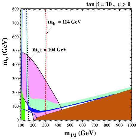
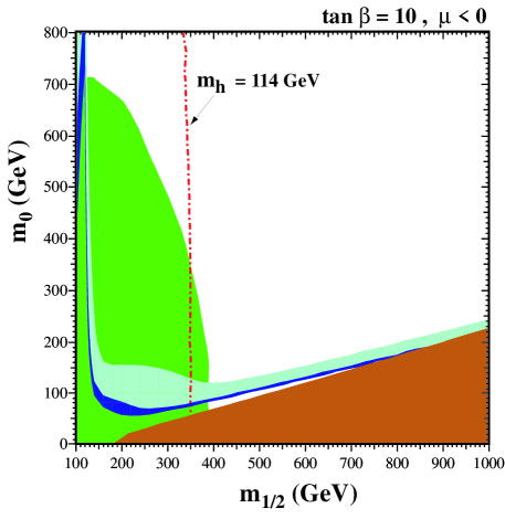
Figure 1: mSUGRA/CMSSM parameter space exclusion plots taken from [396], in which $A_{0}=0$ and other parameters are as shown. The darkest “V” shaped thin strip corresponds to the region with $0.094\leq\Omega h^{2}\leq 0.129$, while a bigger strip with a similar shape corresponds to the region with $0.1\leq\Omega h^{2}\leq 0.3$. (There are other dark strips as well when examined carefully.) The triangular region in the lower right hand corner is excluded by $m_{\widetilde{\tau}_{1}}<m_{\widetilde{\chi}^{0}}$, since DM cannot be charged and hence is a neutralino $\widetilde{\chi}^{0}$). Other shadings and lines correspond to accelerator constraints. In the lower figure ( $\mu<0$), most of the DM favored region below $m_{1/2}<400$ GeV is ruled out by the $b\rightarrow s\gamma$ constraint. In the upper figure, the medium shaded band encompassing the bulge region shows that the region favored by dark matter constraints is in concordance with the region favored by $g_{\mu}-2$ measurements. The Higgs and chargino mass bounds are also as indicated: the parameter space left of these bounds is ruled out. Unless excluded by accelerator constraints, the region below the darkest “V” region is not excluded, but is not cosmologically interesting due to the small relic abundance.

Because of the tight constraints on $\Omega h^{2}$ from the recent WMAP fits [394, 395], a fairly large annihilation cross section is required for compatibility with cosmology. The cosmologically favorable vertical dark strips at $m_{1/2}<105$ GeV are due to s-channel resonance annihilation through the light Higgs and Z poles, and the horizontal strip between $m_{0}=50$ and $m_{0}=200$ GeV is due to coannhilation channels as $m_{\widetilde{\tau}_{1}}$ approaches $m_{LSP}$.

As the masses of the pseudoscalar and the heavy scalar Higgs bosons decrease as $\tan\beta$ increases, s-channel annihilation through very broad Higgs resonance dominates for high $\tan\beta$, giving an acceptable relic abundance. The allowed parameter space through this resonance scattering is sometimes referred to as the funnel region.

There is another often discussed region of parameter space called the focus point region [440], which corresponds to very high values of $m_{0}$, in the multi-TeV range. In this parameter region the LSP becomes more and more higgsino-like due to the falling values of $\mu$ consistent with radiative EWSB. For moderate values of $\tan\beta$, the growing higgsino component opens up new channels for annihilation that can bring down the final dark matter density.

Due to the lower bound on the Higgs mass, most of the mSUGRA parameter space is ruled out. However, the smallness of the allowed regions in the mSUGRA scenario should not be too alarming for considerations of neutralino dark matter. If the universality assumptions of mSUGRA are relaxed, a much larger parameter region becomes viable [455, 456, 457, 458]. Moreover, the smallness of the allowed parameter space also is partly a reflection of the accuracy to which we know the phenomenologically required CDM density. In addition, if there are extra fields such as the axino to which the neutralino can decay, a larger parameter space can become viable, as discussed in Section 6.7. Finally, there can be nonthermal production mechanisms for the LSP.

6.3 Neutralino direct dectection

A great deal of work has been done on both theoretical and experimental aspects of direct detection (see e.g. the reviews [459, 460, 461, 462]). Direct detection of WIMPs can be accomplished through elastic scattering off a nucleus in a crystal [463, 464, 465, 466]. The recoil energy is then measured by a variety of means: scintillation detection, cryogenic detection of phonons (usually relying on superconductor transitions), ionization detection, or some combination thereof. Inelastic nuclear scattering methods have also been considered [467], but most of the proposed experiments use the elastic scattering method due to event rate considerations.

The typical elastic scattering cross section is of the order $10^{-10}$ to $10^{-6}$ pb, and hence the expected event rate is about 1 kg/day or less. The recoil energy of the nucleus is also expected to be very small, of order $10-100$ keV. The background consists of neutrons, $\gamma$-rays, and other cosmic rays. Neutrons are particularly troublesome as the recoil induced by their scattering is difficult to distinguish from the WIMP-induced recoil. Indeed, the background reduction rather than larger exposure remains an important challenge for direct detection experiments.

There are many experiments that have been or will be dedicated to direct detection. DAMA, located in the Gran Sasso underground laboratory, uses 58 kg of NaI [468, 469, 470]; it has already claimed positive detection of dark matter [471] (more below). The CDMS experiment [472, 473], located at the Soundan mine in Minnesota, uses 100 g of Silicon and 495 g of germanium at 20 mK. The EDELWEISS experiment [474], located under the French-Italian Alps, uses three 320 g Ge detectors operating at 17 mK. The ZEPLIN I experiment uses liquid Xenon (a high mass nucleus) corresponding to 4 kg fiducial mass [475] located in Boulby Mine (England). UKDMC NaI [476] is also located in Boulby Mine with a target of around 20 kg. The CRESST experiment utilizes 262 g of sapphire cryogenic calorimeter operating at 15 mK located in the Gran Sasso underground laboratory [477]. Among the future experiments, GENIUS [478] is a particularly prominent experiment progressing in the Gran Sasso underground laboratory which will be able to directly test the DAMA experimental results using 100 kg of natural Ge.

To determine the neutralino direct detection rates, the neutralino-quark elastic scattering amplitudes as well as the one loop neutralino-gluon scattering amplitudes must be computed. The parton level amplitudes are convoluted with quark and gluon distribution functions in nucleons and some model of detector nucleus must be used to account for detector-specific structure effects. This is clearly a large source of uncertainty. Generically, there are both spin-independent and spin-dependent contributions to the elastic cross section.

The spin-independent or scalar part receives contributions from neutralino-quark interactions via squark and Higgs exchange and from neutralino-gluon interactions involving loop quarks, squarks, and Higgses. This can be described in terms of an effective neutralino-nucleon Lagrangian

$${\cal L}_{scalar}=f_{p}\overline{\chi}\chi\overline{\Psi}_{p}\Psi_{p}+f_{n}\overline{\chi}\chi\overline{\Psi}_{n}\Psi_{n},$$ (6.8)

in which the nucleons are denoted by $\Psi_{n,p}$, and the neutralinos are collectively denoted by $\chi$. In the above, the effective couplings $f_{p,n}$ contain all the short distance physics and nucleonic partonic structure information. The differential cross section for scattering on a nucleus of charge $Z$ and atomic number $A$ can then be written as

$$\frac{d\sigma_{scalar}}{d|\vec{q}|^{2}}=\frac{m_{A}^{2}m_{\chi}^{2}}{\pi(m_{A}+m_{\chi})^{2}|\vec{q}|^{2}}\left[Zf_{p}+(A-Z)f_{n}\right]^{2}F^{2}(Q_{r}),$$ (6.9)

where $\vec{q}\equiv m_{A}m_{\chi}/(m_{A}+m_{\chi})\vec{v}$ is the momentum transfer, $Q_{r}=|\vec{q}|^{2}/(2m_{A})$ is the recoil energy, and $F^{2}(Q_{r})$ is the scalar nuclear form factor. Note that the cross section grows with $Z^{2}$ or $(A-Z)^{2}$. There is significant uncertainty in $\{F^{2}(Q_{r}),f_{p},f_{n}\}$ because of the nuclear model sensitivity, and hence the uncertainty should be at least a factor of 2. For intuitive purposes, one may estimate the dimensionless form factor as

$$F^{2}(Q)\sim\exp(-Qm_{N}R_{N}^{2}/3),$$ (6.10)

where $R_{N}\sim 5[0.3+0.91(m_{N}/\textrm{GeV})^{1/3}]$GeV^-1 is the nuclear radius. Similarly, the dimensionful effective nucleon coupling parameters can be estimated as

$$f_{p,n}\sim\left(\frac{m_{p}}{m_{W}}\right)\frac{10^{-1}\alpha_{W}}{m_{H}^{2}}\sim 10^{-8}\textrm{ GeV}^{-2},$$ (6.11)

in which we have assumed that the CP-even Higgs parton level exchange dominates and $m_{H}\sim 100$ GeV is the Higgs mass scale. $\tan\beta$ determines to a large extent which Higgs contribution dominates. In practice, the mass and mixing parameter dependence of these factors are complicated and model dependent; i.e., they are sensitive to the neutralino couplings to Higgs, squarks, and quarks. For further details, see e.g. [479, 467, 461, 428].

The spin-dependent part receives contributions from squark and $Z$ exchange. The effective neutralino-nucleon Lagrangian is

$${\cal L}_{spin}=2\sqrt{2}(a_{p}\overline{\chi}\gamma^{\mu}\gamma_{5}\chi\overline{\Psi}_{p}s_{\mu}\Psi_{p}+a_{n}\overline{\chi}\gamma^{\mu}\gamma_{5}\chi\overline{\Psi}_{n}s_{\mu}\Psi_{n}),$$ (6.12)

where $s_{\mu}$ is the nucleon spin vector and $a_{n,p}$ are the effective theory coefficients. Typically, $a_{n,p}\sim\alpha_{W}/m_{\widetilde{q}}^{2}$ or $\alpha_{W}/m_{W}^{2}$ [479]. The spin interaction differential cross section off of a nucleus with total angular momentum $J$ is

$$\frac{d\sigma_{spin}}{d|\vec{q}|^{2}}=\frac{8m_{A}^{2}m_{\chi}^{2}}{\pi(m_{A}+m_{\chi})^{2}|\vec{q}|^{2}}[a_{p}\frac{\langle S_{p}\rangle}{J}+a_{n}\frac{\langle S_{n}\rangle}{J}]^{2}J(J+1)S_{1}(|\vec{q}|),$$ (6.13)

where $S_{1}(|\vec{q}|)$ is the nuclear spin form factor normalized to $1$ at $|\vec{q}|=0$ for pointlike particles and $\langle S_{p}\rangle$ and $\langle S_{n}\rangle$ represent the expectation values of the proton and neutron spin content in the nucleus. Similar to the spin-independent situation, $\{a_{p},a_{n},S_{1}\}$ have significant model dependence, but these quantities are generally believed to have uncertainties of about a factor of $2$. However, in this case the cross section does not grow with $Z^{2}$ or $(A-Z)^{2}$. Hence, unless the spin content of the nucleus is large, the scalar interactions usually dominate (typically for $A>30$). However, in certain regions of the parameter space, the spin-dependent part can play a significant role even when $A>30$. For example, for ${}^{73}\textrm{Ge}$, which has a nonzero nuclear spin of $J=9/2$, the spin-dependent contribution can give a significant contribution for $\mu<0$ and moderate values of $\tan\beta$. Although not well-determined, one can approximate $\langle S_{p}\rangle\approx 0.03$ and $\langle S_{n}\rangle\approx 0.378$ [480].

The differential detection rate is given by

$$\frac{dR}{dQ_{r}} = \frac{4}{\sqrt{\pi^{3}}}\frac{\rho_{\chi}}{m_{\chi}v_{0}}T(Q_{r})\left\{[Zf_{p}+(A-Z)f_{n}]^{2}F^{2}(Q_{r})\right.$$ (6.14)

$$\left.+8[a_{p}\frac{\langle S_{p}\rangle}{J}+a_{n}\frac{\langle S_{n}\rangle}{J}]^{2}J(J+1)S_{1}(|\vec{q}|)\right\},$$

in which $v_{0}\approx 220$ km/s is the speed of our sun relative to the center of the galaxy, $\rho_{\chi}$ is the local LSP density, and

$$T(Q_{r})=\frac{\sqrt{\pi}v_{0}}{2}\int_{v_{min}}^{\infty}dv\frac{f_{\chi}(v)}{v}$$ (6.15)

integrated over the neutralino velocity distribution $f_{\chi}$. The recoil energy $Q_{r}$ is typically no more than $100$ keV. The greatest uncertainty in the differential detection rate is from the uncertainty in the local LSP density $\rho_{\chi}$ [481, 482, 483, 484, 485, 486, 487, 488, 489, 490, 491, 492, 493]; the answer is uncertain by a factor of a few. When folded in with the nuclear physics uncertainties, the final theoretical detection rate is uncertain by about a factor of 10 or more.

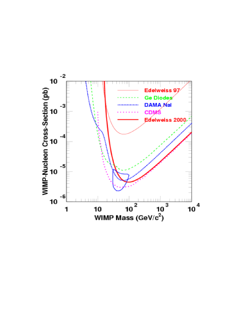
Figure 2: Typical exclusion plot taken from [494]. The region above the curves are excluded. The closed curve represents the $3\sigma$ positive detection region of DAMA experiment.

One way to enhance the detection signal above the background is to look for modulations in the signal rate due to the detector’s time varying velocity relative to the dark matter halo. For example, due to the earth’s motion around the sun, the time of the maximum velocity of the dark matter halo with respect to the terresterial detector is six month separated from that of the minimum velocity of the dark matter halo with respect to the terresterial detector [466, 495]. This method has been the focus of the DAMA experiment [468, 469, 470], which has announced positive detection of the annual modulation [471]. However, the discovery has been disputed by many experimental groups and has still neither been undisputedly excluded nor confirmed [496], despite many questionable claims to the contrary in the literature.

Another way to enhance the signal above the background is to resolve the nuclear recoil direction as the dark matter elastically scatters [497]. Because of the strong angular dependence, generically the number of recoil events in the forward direction will significantly exceed the number of events in the backward direction for any energy threshold of the detector. Due to the daily rotation of the earth, the detector should then see a modulation between the nighttime and the daytime (diurnal modulation). The proposed experiment DRIFT [498] is thus far the only experiment that has enough directional sensitivity to take advantage of diurnal modulation. On the other hand, because this experiment relies on measuring ionization tracks in a low pressure gas, one drawback is the low target mass required by the low pressure gas.

It has been argued that prospects for the discovery of supersymmetry through the direct detection of LSP CDM are as good as or better than through detection at the LHC (see e.g. [499]) in some regions of parameter space, such as the focus point region. A typical exclusion plot for data that has already been taken can be seen in Figure 2. Of course, because different detectors have different energy thresholds and detection techniques, one must be careful to consider the details of the experiments before drawing conclusions from these kinds of plots. Furthermore, recall from our previous discussion that there is about a factor of 10 uncertainty in the final detection rate. Given that this is an active area of experimental research, we expect to see substantial improvements in the near future.

6.4 Neutralino indirect detection

The indirect detection processes are classified according to which particles are actually interacting with the laboratory detector. The detected particles are generally cosmic ray particles resulting from the annihilation of LSP neutralinos. We will first discuss neutrino telescopes, which arguably have the least number of astrophysical uncertainties, and then mention the detection of other cosmic ray particles.

Neutrino Telescopes

LSP dark matter can accumulate in astrophysical bodies such as the sun or the earth by elastic scattering if the final state WIMPs have velocities less than the escape velocity [500, 501, 502]. The accumulated LSPs can annihilate, giving rise to observable final products. Among the SM decay products of the primary annihilation products, the muon neutrino can escape without being absorbed by the core of the sun or the earth and can reach terresterial detectors. Since $\chi\chi\rightarrow\nu\nu$ is suppressed by the small neutrino masses, the neutrinos primarily arise due to decays of primary products of annihilation with a mean energy of $\sim m_{\chi}/2$. In the water/terrestrial material immersing the detectors, the muon neutrinos induce muon production, which can easily be measured by its Cerenkov radiation.

The derivation of the capture rate (number per unit time) starts by writing the differential scattering events per unit time as

$$d\dot{N} = (\#\textrm{ of nuclei })\times(\textrm{velocity differential flux})\times$$ (6.16)

$$(\textrm{angular diff}\textrm{erential elastic cross-section onto one nucleus}).$$

One then does the angular integration, restricting the final angle such that the final state particle is below the escape velocity, and performs the summation over the appropriate nuclei distributions. Thus computed, the capture rate of neutralinos in an astrophysical body of mass $M$ (recall the mass of the sun is $M=1.1\times 10^{57}$ GeV and the mass of the earth is $M=3.4\times 10^{51}$ GeV) can be written as [502, 503, 504, 505]

$$C\sim\frac{\rho_{\chi}}{v_{\chi}}M\sum_{i}f_{i}\frac{\sigma_{i}}{m_{\chi}m_{i}}\langle v_{\textrm{esc }}^{2}\rangle_{i}S(v_{\chi},v_{\textrm{esc }},m_{\chi},m_{i}),$$ (6.17)

where $\rho_{\chi}$ and $v_{\chi}$ denote the local neutralino density and speed, $f_{i}$ is the fraction of nucleus $i$ in the astrophysical body, $v_{\textrm{esc}}$ is the escape speed, $\langle...\rangle$ denotes averaging over the distribution of the element $i$, $\sigma_{i}$ is the nucleus-LSP elastic scattering cross section, and $S(...)$ is a suppression factor which accounts for the additional kinematics of the neutralino-nucleus interaction. Typically, $\rho_{\chi}\sim 3\times 10^{-42}$ GeV⁴, $v_{\chi}\sim 10^{-3}$, and $v^{2}_{esc}\sim(4\times 10^{-5})^{2}$ for the earth while it is $v_{esc}^{2}\sim 10^{5}(4\times 10^{-5})^{2}$ for the sun.

Because the local speed after the elastic scattering is [502, 506]

$$v^{2^{\prime}}=v^{2}\left(1-\frac{2m_{\chi}m_{i}}{(m_{i}+m_{\chi})^{2}}[1-\cos\theta_{\textrm{cm }}]\right),$$ (6.18)

where $\theta_{\textrm{cm }}$ is the center of mass scattering angle, there is a greater loss of energy after scattering when $m_{\chi}\approx m_{i}$ (and hence a “resonant” enhancement [502] in the capture rate). Because the earth has heavy elements, there is a resonant enhancement of capture for the mass range

$$10\textrm{ GeV}\leq m_{\chi}\leq 75\textrm{ GeV},$$ (6.19)

with the peak near the iron mass of $m_{Fe}\approx 56$ GeV.

Although the sun does not have such heavy elements to cause resonant scattering, the large quantity of the sun’s hydrogen carries spin, allowing axial interactions to become important. Such interactions are particularly important if there is significant $Z$ coupling, which in turn depends on the higgsino fraction of the neutralino. Due to the large solar mass and this spin-dependent neutralino-quark cross section ($\sigma_{\chi p}^{\textrm{scalar}}<\sigma_{\chi p}^{\textrm{spin }}$), the solar capture of the neutralinos is usually much more efficient than neutralino capture in the earth.

Given the capture rate of Eq. (6.17), the annihilation rate into neutrinos and the resulting neutrino flux near the detector must be calculated. Following [507], the annihilation rate can be deduced from the simplified Boltzmann equation (neglecting evaporation):

$$\dot{N}_{\chi}=C-C_{A}N_{\chi}^{2},$$ (6.20)

where $N_{\chi}$ is the number of neutralinos, and

$$C_{A}\approx\frac{\langle\sigma_{A}v\rangle}{V_{0}}\left(\frac{m_{\chi}}{20\textrm{ GeV}}\right)^{3/2}$$ (6.21)

is the annihilation rate per effective volume of the body, with $V_{0}\sim 2.3\times 10^{25}\textrm{cm}^{3}(\approx 3\times 10^{66}\textrm{ GeV}^{-3})$ for the earth and $V_{0}\sim 6.6\times 10^{28}\textrm{ cm}^{3}(\approx 8.6\times 10^{69}\textrm{ GeV}^{-3})$ for the sun. Assuming that $C$ and $C_{A}$ remain constant, the total annihilation rate is

$$\Gamma_{A}=\frac{1}{2}C_{A}N_{\chi}^{2}=\frac{C}{2}\tanh^{2}[t\sqrt{CC_{A}}],$$ (6.22)

where $t\approx 4.5$ Gyr ($\approx 2.2\times 10^{41}$GeV^-1) is the age of the macroscopic body. When accretion is efficient such that $\tanh^{2}\approx 1$, the annihilation rate $\Gamma_{A}$ is independent of the annihilation cross section, but dependent on the capture rate $C$. For the sun, the neutralinos are nearly in “equilibrium” due to the large capture rate implying $\Gamma_{A}\approx C/2$. However, when the higgsino component is small, for example as in the low $m_{0}$-high $m_{1/2}$ region of mSUGRA parameter space, $\Gamma_{A}$ has a $C_{A}$ dependence. Also, $C_{A}$ is smaller when $\tan\beta$ is low, enhancing the $C_{A}$ sensitivity of $\Gamma_{A}$. For the earth, neutrinos are not in equilibrium due to the generally smaller capture rate, leading to $\Gamma_{A}$ of the form

$$\Gamma_{A}\sim\frac{C^{2}C_{A}t^{2}}{2}.$$ (6.23)

This leads to enhancements in parameter regions where the annihilations are large, as discussed in Section 6.2.

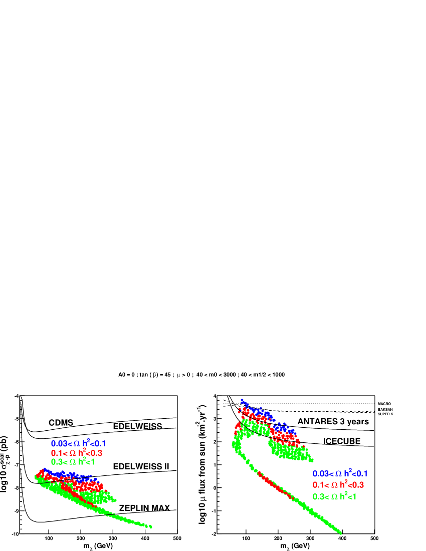
Figure 3: Taken from [508], the left figure shows the direct detection scalar elastic scattering cross section for various neutralino masses, and the right figure shows the indirect detection experiments’ muon flux for various neutralino masses. The scatter points represent “typical” class of models. Specifically, the model parameters are $A_{0}=0,\tan\beta=45,\mu>0,m_{0}\in[40,3000],m_{1/2}\in[40,1000].$ The dotted curve, dot dashed curved, and the dashed curve on the right figure represents the upper bound on the muon flux coming from Macro, Baksan, and Super-Kamiokande experiments, respectively. This plot should be taken as an optimistic picture, because the threshold for detection was set at 5 GeV, where the signal-to-noise ratio is very low in practice.

Given $\Gamma_{A}$, the neutrino differential flux is

$$\frac{d\Phi}{dE}=\frac{\Gamma_{A}}{4\pi R^{2}}\sum_{j}b_{j}\left(\frac{dN}{dE}\right)_{j},$$ (6.24)

where $R$ is the detector-(neutralino source) distance, $b_{j}$ is the branching ratio of annihilation channel $j$, and $dN/dE$ is the differential neutrino spectrum. As mentioned previously, the smallness of the neutrino mass suppresses annihilation channels directly to neutrinos, and electron neutrinos scatter too efficiently to reach the detector from the source. Therefore, the neutrino-producing reactions of interest are secondary particle decays. The hard (energetic) muon neutrinos come from $WW$, $ZZ$, and $t\overline{t}$ decays (assuming the neutralino mass is above these thresholds), while the soft muons neutrinos are sourced by $b\overline{b}$ decays. Since muons are the actual particles being detected and neutrino-induced production of muons grows with the neutrino energy, high energy neutrinos are easier to detect. This means that the muon flux will be larger for larger neutralino masses, which roughly translates to larger $m_{1/2}$ in mSUGRA. Also, since an enhanced higgsino component increases the annihilation into $WW$ and $ZZ$ which gives more energetic neutrinos, increasing the higgsino component of the neutralino enhances the muon signal as well. Although the ratio of the mass of the sun to the mass of the earth is around $3\times 10^{5}$ and the distance-squared ratio between the earth-sun distance and the earth radius is around $5\times 10^{8}$, because $\langle v_{esc}^{2}\rangle$ is also proportional to $M$ and the spin-dependent cross section is larger than the scalar cross section, the flux of neutrinos originating from the earth is typically much smaller than the flux originating from the sun.

The uncertainties in the theoretical calculations should be similar to the direct detection case, since the quantities that enter are similar: i.e., most of the uncertainties stem from local astrophysics. For example, even a small deviation from the usually assumed Maxwellian distribution of neutralinos (caused by scattering with the sun and interacting with large planets) can have an $O(100)$ effect on the indirect detection rates due to annihilation in the earth for $m_{\chi}<150$ GeV [509].

There have been several experiments under the category of neutrino telescopes which had put bounds through indirect detection, including Macro [510], Baksan, Super-Kamiokande, and AMANDA [511]. Future experiments have potential to indirectly detect the neutralinos. One is the Antares 0.1 km² project which covers a volume of around 0.02 km³ (which may be upgraded upgraded to 1 km³ in the future) in the Mediterranean sea at a depth of 2.4 km down south of France. Another project, ICECUBE, will cover 1 km³ volume under about 2.4 km of ice [512, 513]. The reaches of these experiments are compared to the direct detection experiments in Figure 3. The typical energy thresholds are between 5 to 10 GeV.

Other cosmic rays

In addition to the neutrino telescopes, there may also be the possibility possibility of indirect neutralino detection through other cosmic ray particles [514]. Examples include gamma rays [514, 515, 516, 517, 518, 519, 520, 521, 522, 523, 524, 525, 526], lower energy photons such as radiowaves [516, 527], and antimatter such as positrons and antiprotons [514, 528, 529, 530, 531, 532, 533, 534, 535]. The source of these cosmic rays will be concentrated towards the center of our galaxy. In fact, the recent positron excess reported by the HEAT balloon borne experiment [536, 537, 538] may be attributable to WIMP annihilations if certain nonstandard astrophysical phenomena are assumed to take place [531, 539, 540, 541, 542]. Specifically, the HEAT collaboration has reported an excess of positrons that are consistent with arising from LSP annihilation if the LSP is heavier than the W. While further study is needed to argue that this excess does not arise from conventional sources, there has not been a convincing alternative scenario which leads to an excess with a peak at an energy of order 10 GeV. The excess has been seen in several sets of data with different detectors.

As far as theoretical predictions are concerned, there is greater uncertainty in the non-neutrino signals since they involve greater model dependence of the galactic halo. For example, consider the photons. The computation of the differential flux is usually done using the approximate formula

$$\frac{dF_{\gamma}}{d\Omega dE}=\sum_{i}\frac{dN_{\gamma}^{i}}{dE}\sigma_{i}v\frac{1}{4\pi}\int n_{\chi}^{2}dl,$$ (6.25)

where $dl$ is the line of sight integral, $dN_{\gamma}^{i}/dE$ is the photon spectrum injected per annihilation channel $i$ (this includes any secondary particle decay probability), $\sigma_{i}v$ is the usual annihilation cross section times the Moeller speed factor, and $n_{\chi}$ is the neutralino density in the halo. The strong model dependence is in the $n_{\chi}^{2}$ integral. The fiducial value is usually taken to be

$$\int n_{\chi}^{2}dl\sim\left(\frac{0.3\textrm{GeV}}{m_{\chi}}\frac{1}{\textrm{cm}^{3}}\right)^{2}(8.5\textrm{kpc}),$$ (6.26)

which corresponds to the critical density being made up by the dark matter, and $8.5$ kpc is the distance of the sun from the Galactic center. There is at least a factor of $10^{3}$ (perhaps even as large as $10^{5}$) uncertainty in this integral [519]. The line signal (neutralino annihilation directly into photons [543, 544, 545, 546]) is a loop-suppressed process and is generically smaller relative to the continuous spectrum signal (dominated by $\pi^{0}\rightarrow\gamma\gamma$) in the parameter region of interest. On the other hand, because it is difficult to mimic a line signal by astrophysical processes not involving heavy WIMPs, the line signal is more robust in terms of being able to claim discovery of a heavy relic.

The positron flux predictions stem from a equation similar to Eq.(6.25), except with an additional convolution of a nontrivial Green’s function for the positron propagation. On the other hand, because only the high energy positrons (with energies above the soft positrons coming from the solar wind) are easily measurable above the background and since the high energy positrons lose energy efficiently, the source of measurable positron flux cannot be as far away as the galactic center, and instead must be within a few kpc of the earth. This makes the calculation less sensitive to the uncertainties of the matter distribution at the galactic center compared to the photon case. The positron flux can then be written as

$$\frac{dF_{e^{+}}}{d\Omega dE}=n_{\chi}^{2}(x_{0})\sum\sigma_{i}v\int dE^{\prime}\frac{dN_{e^{+}}^{i}(E^{\prime})}{dE^{\prime}}G(E,E^{\prime}),$$ (6.27)

where $n_{\chi}^{2}(x_{0})$ is the local neutralino density, $\frac{dN_{e^{+}}^{i}(E^{\prime})}{dE^{\prime}}$ is the positron injection spectrum at the neutralino annihilation source, and $G(E,E^{\prime})$ embodies the propagation of the postirons and any remaining uncertainties in the halo profile models. An example of $G(E,E^{\prime})$ for a “leaky box” toy model [528, 529, 530] is

$$G(E,E^{\prime})\approx\frac{1}{4\pi\xi}\frac{1}{E^{2}}\theta(E^{\prime}-E)e^{\frac{E^{{}^{\prime}-1}-E^{-1}}{\tau_{0}\xi}},$$ (6.28)

which at best can give a reasonable order of magnitude estimate with $\xi=1.11\times 10^{-9}\textrm{yr}^{-1}\textrm{GeV}^{-1}$, $\tau_{0}=10^{7}\textrm{ yr}$. For a better model and further discussions, see [531].

Regarding photon detection, among the various future experiments the outer space experiment GLAST will have the greatest sensitivity and will have a good chance of seeing a signal because of its wider angular acceptance and better energy resolution and reach [547]. As previously stated, the most clean signal is the line (narrow width) spectral signal, which corresponds to at least one of the primary annihilation products of the neutralinos being a photon. Other photon-sensitive experiments that have already run or are planning to run include STACEE, CELESTE, ARGO-YBJ, MAGIC, HESS, VERITAS, AGILE, CANGAROO, and AMS/$\gamma$. The most promising experiments as far as the positron (and other antimatter) signal is concerned are the space borne experiments PAMELA [535] and AMS-02 [537], both of which are sensitive to high positron energies, as large as 200 and 1000 GeV. Unfortunately, the positron signal-to-background ratio is generically extremely low, typically less than $0.01$ [441]. An antiproton signal also must fight a large background [548, 549, 526, 550].

6.5 Complementarity

Not surprisingly, direct detection, indirect detection, collider detection, and constraints from SM precision data play complementary roles — mutually checking as well as having different parameter reaches — in the search for supersymmetry. This can be understood by examining the schematic dependence on physical quantities controlling the magnitude of the direct and indirect signals, as shown in Table 6.

	p-elastic	low $\sqrt{s}$ annhilation	abundance	error
direct detection	$\sigma_{\chi p}$		$n_{\chi}(\textrm{local})$	$10$
neutrino telesc.	$\sigma_{\chi p}$	little for sun	$n_{\chi}(\textrm{local})$	$10$
$\gamma$ (line, continuum)		$\sigma_{\chi\chi\rightarrow\gamma X},\sigma_{\chi\chi\rightarrow\pi^{0}\pi^{0}}$	$n^{2}_{\chi}(\textrm{core})$	$10^{3}$
$e^{+}(E>10\textrm{ GeV})$		$\sigma_{\chi\chi\rightarrow WW,ZZ}$	$n_{\chi}^{2}(\textrm{nearby})$	$100$
collider	$\sigma_{\chi p}$	$\sigma_{\chi\chi\rightarrow XX}$	small	small

Table 6: A schematic picture of the various search processes. The column labeled “p-elastic” gives the dependence on proton-neutralino elastic-cross section; “low $\sqrt{s}$ annihilation” refers to the dependence on various self-annihilation cross section at very low momenta (characteristic of the dark matter temperature in the halo); $n_{\chi}(\textrm{local})$ refers to the density of the neutralinos in our solar system; $n_{\chi}(\textrm{core})$ refers to the density at the center of the galaxy; $n_{\chi}(\textrm{nearby })$ refers to the halo density within few kpc of the solar system (not at the core of the galaxy). The “error” refers to a minimal multiplicative uncertainty in the theoretical predictions. The table is not precise for all parts of the MSSM parameter space and is merely meant to provide an elementary picture of the typical situation. Collider data obviously does not directly involve the proton-neutralino elastic cross section nor the self-annihilation cross section at nonrelativistic energies. However, collider sensitivity generically is enhanced with light superpartners, which also tend to enhance both the elastic and the self-annihilation cross sections.

Collider and electroweak precision searches prefer lighter superpartners. In mSUGRA, this corresponds to smaller $m_{0}$ and $m_{1/2}$ parameters. On the other hand, indirect searches are typically enhanced for a larger higgsino component, which in mSUGRA corresponds to the large $m_{0}$ region. In fact, if the LSP has a large higgsino component and is heavier than a few TeV, the detection of gamma rays through the $\chi\chi\rightarrow\gamma\gamma$ and $\chi\chi\rightarrow\gamma Z$ channels [462] may be the only way to discover supersymmetry in the foreseeable future because the accelerator, direct detection, and indirect neutrino dection may not have the required sensitivities. Of course, such heavy neutralinos may be disfavored from fine-tuning arguments. Even for such large mass neutralinos, the annihilation can be strong enough to not overclose the universe if there is a sufficient higgsino component. The direct detection searches, which are sensitive to $\sigma_{\chi p}$, have an inverse correlation in some regions of the parameter space with the indirect detection searches through $\sigma_{\chi\chi\rightarrow\gamma\gamma}$, as higgsino-like neutralino models with $m_{\chi}>400$ GeV which have a small $\sigma_{\chi p}$ generally have large $\sigma_{\chi\chi\rightarrow\gamma\gamma}$ [462].

The neutrino telescope searches tend to complement the direct detection searches by having some overlap in sensitivity, as both are very sensitive to $\sigma_{\chi p}$ [551]. In fact, there is a possibility of measuring $m_{\chi}$ by detecting the angular distribution of the muons in the neutrino telscope [552, 553].

Generically, there is an inverse correlation of the elastic scattering cross section with the cosmological relic abundance of the neutralinos. By looking at Table 6, one would then naively conclude that the direct detection process and indirect detection to some extent can still detect neutralinos even if neutralino LSPs did not dominate the CDM composition. Indeed, direct dark matter searches have sensitivity in both the light LSP and the heavy LSP region, as can be seen in Figure 2. Even for the indirect detection, [554] demonstrates that an LSP halo fraction as small as 1% can be indirectly detected with the current generation of experiments.

However, collider measurements of LSP neutralinos and their couplings relevant for self-annihilation do not imply that the dark matter abundance can be computed, because R-parity violation, light axinos (see Section 6.7), or a low reheating temperature may spoil the standard LSP dark matter scenario. In practice, even within the standard cosmological scenario, the situation with collider measurements alone is even worse than what it naively would seem because the relevant parameters needed to calculate the relic density must be measured to an accuracy of order 5% to obtain a useful answer for the relic density [555].

Remarkably, even with LHC discovery of supersymmetry and LSP neutralinos and with the assumptions of a standard cosmological scenario and R-parity conservation, we still may not be able to know whether the bulk of the CDM is composed of LSP neutralinos. Hence, direct and indirect detection of dark matter are important to ascertain the identity and the fraction of CDM in LSP neutralinos. On the flipside, having direct and indirect detection of the LSP neutralino dark matter by themselves do not specify the fraction of CDM in LSP neutralinos because the local astrophysical uncertainties are unlikely to be smaller than a factor of 2 in the near future and because the relevant ${\mathcal{L}}_{soft}\,\,$parameters must be measured to interpret the detection meaningfully. Therefore, very accurate collider and other measurements of the parameters that are essential for the relevant kind of dark matter which can allow computations of Section 6.1 are essential to determine the LSP fraction of the CDM. This will most likely require colliders beyond the LHC.

6.6 Gravitinos

In scenarios such as gauge-mediated supersymmetry breaking, the gravitino naturally is the LSP, and hence becomes a dark matter candidate [23, 556]. For example, if the supersymmetry-breaking scale is of order $\sqrt{F}\sim 10^{6}$ GeV, the gravitino mass is of the order $F/\overline{M}_{pl}\sim 10^{-6}$ GeV ($F$ is the F term VEV which characterizes supersymmetry breaking, as discussed in Section 3). The helicity $1/2$ (goldstino) component has gravitational interactions of dimension 4 and 5, with coefficients of the order $(m_{\chi}^{2}-m_{\phi}^{2})/(m_{3/2}\overline{M}_{pl})$ and $m_{\lambda}/(m_{3/2}\overline{M}_{pl})$ [557] (here $m_{\phi}$ and $m_{\lambda}$ denote scalar and gaugino masses, respectively). This allows it to interact much more strongly when $m_{\lambda,\chi,\phi}\gg m_{3/2}$ than the helicity $3/2$ component, for which the gravitational interactions are not similarly enhanced. Without this enhancement, as in e.g. gravity-mediated supersymmetry breaking scenarios in which $m_{3/2}\sim O(\textrm{TeV})$, gravitinos never reach thermal equilibrium below Planck scale temperatures. The enhancement allows thermal equilibrium to be reached, such that the gravitinos can go through the usual freeze out process to act as warm dark matter candidates. The relic abundance can be calculated as

$$\Omega_{\widetilde{g}(th)}h^{2}\approx\left(\frac{m_{3/2}}{1\textrm{ keV}}\right)\left(\frac{g_{*}(T_{f})}{100}\right)^{-1},$$ (6.29)

which requires $m_{3/2}$ to be less than about $0.1$ keV if the Hubble parameter today is given by $h\approx 0.7$ and $g_{*}(T_{f})=100$. This may cause problems in the context of gauge mediation [23, 558, 559], because such low values for the $F$ term are unattractive in some gauge-mediated models. One may need to invoke methods to dilute the gravitino abundance [560] or have a low reheating temperature [558, 559]. In certain special arrangements of the sparticle mass spectrum, there can be a secondary population of nonthermal gravitinos from NLSP decay [561]. Due to their nonthermal momentum distribution, this secondary population can mimic hot dark matter consisting of eV range neutrinos. There are other ways to generate a nonthermal distribution of gravitinos as well [562, 563, 564]. Even when the reheating temperature is small enough that there is no overclosure of the universe with LSP gravitinos, there may be a cosmological problem with the decay of NLSPs (which typically have long lifetimes) into gravitinos, because such decays are generally accompanied by decay products which can spoil big bang nucleosynthesis (BBN) [565, 566, 567, 568, 569, 570, 571, 572, 573].

Figure 4: Reheating temperature upper bound constraints from BBN as a function of the gravitino mass taken from [572]. The various “high” and “low” values refer to the usage of observationally deduced light nuclei abundances in deducing the upper bound. Hence, the discrepancy can be seen as an indication of the systematic error in the upper bound constraint from observational input uncertainties.

In gravity-mediated supersymmetry-breaking scenarios, the mass of the gravitino is generically close to a TeV and it usually is not the LSP. In such scenarios, there may be several cosmological problems caused by gravitino decay products which can dissociate nuclei during BBN, destroying its successful predictions [567, 574, 566, 568, 570, 572, 569, 575, 576]. In general, successful BBN requires the photons to have a nearly thermal spectrum, while the gravitino decay products may induce sufficient departures from the thermal spectrum to ruin the successful ratios of element abundances. The disruption of the photon spectrum can occur through primary decay products as well through particles farther down the cascade of reactions. Assuming that the gravitino decays to a photino and a photon, its lifetime is given by [567]

$$\tau_{3/2}=3.9\times 10^{8}\left(\frac{m_{3/2}}{100\textrm{ GeV}}\right)^{-3}\textrm{ sec}.$$ (6.30)

The decay has a long time scale because it originates from a dimension five ($1/M_{Pl}$ suppressed) operator. For reference, BBN occurs during $\tau_{BBN}\approx 1-10^{2}$ sec ($T\approx 1-0.1$ MeV).

Assuming the gravitinos are produced thermally (although they never reach thermal equilibrium unless $m_{3/2}\ll 100$ GeV), the gravitino abundance can be calculated as a function of the reheating temperature of the universe $T_{RH}$ to be [567]

$$\frac{n_{3/2}}{n_{\gamma}}\approx 2.14\times 10^{-11}\left(\frac{T_{RH}}{10^{10}\textrm{GeV}}\right)$$ (6.31)

for $T\ll 1$ MeV but for time $t<\tau_{3/2}$. This is a significant number and energy density since the baryon-to-photon ratio is $n_{B}/n_{\gamma}\sim 10^{-10}$ and $m_{3/2}\gg m_{p}$. This large number of gravitinos will decay to photons, which will cause the dissociation of BBN nuclei through reactions such as $D+\gamma\rightarrow n+p$ or ${}^{4}He+\gamma\rightarrow n+^{3}He$ . An example of bounds coming from successful BBN can be seen in Figure 4.

6.7 Axion, axino, and saxion

As discussed previously, the axion field $a$ is a pseudo-Nambu-Goldstone boson of the broken $U(1)_{PQ}$ symmetry which solves the strong CP problem; its presence changes the usual $\overline{\theta}$ to

$$\overline{\theta}_{a}=\overline{\theta}-\frac{a(x)}{f_{PQ}/N},$$ (6.32)

where $f_{PQ}$ is the PQ breaking scale and $N$ is defined below. Its properties depend most strongly on only one unknown parameter, the axion mass $m_{a}$ or equivalently the PQ breaking scale $f_{PQ}$:

$$m_{a}\approx\frac{\sqrt{Z}}{1+Z}\frac{f_{\pi}m_{\pi}}{(f_{PQ}/N)},$$ (6.33)

where the pion decay constant is $f_{\pi}\approx 93$ MeV, the pion mass is $m_{\pi}\approx 135$ MeV, the dimensionless ratio $Z\equiv m_{u}/m_{d}$, and $N=\textrm{Tr}[Q^{PQ}(Q^{\alpha}_{\textrm{SU}(3)_{C}\textrm{ }})^{2}]$ is the color anomaly of the PQ symmetry [367, 577, 578, 361, 378, 579]. Its interactions include its coupling to the gluon

$$\frac{\alpha_{3}g_{agg}}{8\pi}\frac{a}{(f_{PQ}/N)}\widetilde{G}^{a}_{\mu\nu}G^{\mu\nu}_{a},$$ (6.34)

the nucleon and electron

$$i\frac{1}{(f_{PQ}/N)}\partial_{\mu}a\left[g_{ann}(\overline{n}\gamma^{\mu}\gamma_{5}n)+g_{aee}(\overline{e}\gamma^{\mu}\gamma_{5}e)\right],$$ (6.35)

and the photon

$$\frac{\alpha_{EM}g_{a\gamma\gamma}}{2\pi}\frac{a}{(f_{PQ}/N)}\widetilde{F}^{\mu\nu}F_{\mu\nu}$$ (6.36)

where $g_{aii}$ are model-dependent $O(1)$ coefficients. Two standard models of axions are the KSVZ [369, 371] and DFSZ [372, 370] models. Models such as KSVZ models with $g_{aee}=0$ at tree level are called “hadronic” because they lack direct couplings to leptons. As all the couplings are suppressed by ${\rm momentum}/(f_{PQ}/N)$, the axion can be essentially “invisible” if $f_{PQ}/N$ is large enough. However, as will be explained below, $f_{PQ}/N$ is severely constrained by various measurements.

Since the interaction strength becomes larger as $f_{PQ}/N$ is lowered, the lower bound on $f_{PQ}/N$ is determined both indirectly and directly by observable particle reactions that can produce axions [580, 581]. One example is Supernova 1987A (SN1987A) which yielded a total of 19 detected neutrino events spanning a time period of about 12 seconds which was in accord with the expectations. For axions in the mass range $f_{PQ}/N\approx 4\times 10^{9}$ GeV to $f_{PQ}/N\approx 2\times 10^{6}$ GeV, the cooling due to axion emission through bremsstrahlung from nucleons would shorten the duration of the neutrino emission to unacceptable values much smaller than 12 seconds, according to the standard picture [582]. The main reason why SN cannot rule out smaller values of $f_{PQ}/N$ is because at these smaller values, the interactions become sufficiently strong such that the axions become trapped in the supernova core, causing the axion-mediated cooling to be inefficient. For smaller $f_{PQ}/N$, stellar processes provide constraints. Axion emission from the stellar core accelerates stellar evolution (more intense burning to compensate for the axion emission energy loss), shortening the lifetime of red giants. For hadronic axions, this gives a bound of $22\textrm{ GeV}<f_{PQ}/N<9\times 10^{6}\textrm{ GeV}$ [583, 584, 585]. The lower bound is due to the red giant core temperature scale of $10$ keV being too small to excite heavier axions. The upper bound is from the requirement of the axion being sufficiently strongly coupled to be produced. Because the He core is supported by the electron degeneracy pressure for the DFSZ type of axions, the axion coupling to the electrons can cool the He core to such an extent that the He burning never takes place [586]. This extends the upper bound from red giants on $f_{PQ}/N$ to $22\textrm{ GeV}<f_{PQ}/N<4\times 10^{8}$GeV. Finally, for even more strongly coupled, heavier axions, a variety of lab experiments [587] put constraints of $f_{PQ}/N>86$ GeV. Therefore, the combined experimental results exclude a broad range of scales, leading to a lower bound on the axion scale of $f_{PQ}/N>4\times 10^{9}$ GeV.

The upper bound on $f_{PQ}/N$ is given by cosmology from dark matter constraints. Since axions have a long lifetime

$$\tau_{a}\sim 10^{17}\textrm{ yrs }\left(\frac{m_{a}}{1\textrm{ eV}}\right)^{-5},$$ (6.37)

axions can be good dark matter candidates. The long lifetime compared to that of the pion is due to the enhancement $(m_{\pi}/m_{a})^{5}$. The cosmology of axions depends on the inflationary history of the universe: we will assume throughout this review that inflation took place. If inflation reheats to a temperature larger than the lower bound of $f_{PQ}/N$ of $4\times 10^{9}$ GeV, gravitinos tend to disrupt the successes of standard cosmology (see Section 6.6). Furthermore, if the reheating temperature is above $f_{PQ}$, there may be a problem with domain wall formation; this leads to at best a complicated, more model-dependent cosmology [588]. To keep the model dependence down and the physics simple for this review, we will focus on situations where the reheating temperature is lower than the PQ transition. Even then, there are inflationary model dependent constraints due to the quantum fluctuations of the axion field during inflation [589, 590], which we will not discuss here.

Because the interaction rate is extremely small (e.g., for quark mass $m_{q}$, $\langle\sigma v\rangle\sim\alpha(m_{q}/(f_{PQ}/N))^{2}/T^{2}$ for $T>m_{q}$, which is again strongly suppressed by $f_{PQ}/N$), the axions typically cannot be in thermal equilibrium for $f_{PQ}/N>4\times 10^{9}$ GeV [591]. Furthermore, one can estimate that the relic density of thermally produced axions will be a negligible component of the CDM, typically close to the energy density contribution of the cosmic microwave background (CMB) radiation. However, axions can be a large source of CDM from the condensate oscillation contribution, i.e. essentially, homogeneous classical axion field oscillations in time. The reason why the axion field will generically have such oscillations is that before the QCD phase transition, the axion has a relatively flat potential, such that its value (call it $a_{i}$) can be anywhere of $O(f_{PQ})$. After the QCD phase transition, instanton effects will generate a potential for $a$. Since the minimum of the potential $a_{m}$ will be different from $a_{i}$, the axion will undergo a damped oscillating motion about the minimum of the potential with the maximum initial amplitude of $a_{i}-a_{m}$. This oscillation will contribute an energy density [592, 593, 594, 595, 596]

$$\Omega_{a}\approx\frac{1}{6}\left(\frac{a_{i}-a_{m}}{f_{PQ}/N}\right)^{2}\left(\frac{f_{PQ}/N}{10^{12}\textrm{GeV}}\right)^{7/6}\left(\frac{0.7}{h}\right)^{2},$$ (6.38)

which would generically give a large contribution if $f_{PQ}$ is large with the oscillation amplitude $(a_{i}-a_{m})/(f_{PQ}/N)$ fixed (which naively is naturally expected to be of $O(1)$). In the absence of fine tuning $a_{i}$, the $U(1)_{PQ}$ breaking scale is then bounded to be $f_{PQ}/N<10^{12}\textrm{GeV}.$ Therefore, remarkably, the scale of new physics is known to be within a small window

$$10^{9}\textrm{GeV}<f_{PQ}/N<10^{12}\textrm{ GeV}.$$ (6.39)

However, there is some room for adjustment (particularly at the upper end), if there is a method to relax $a_{i}$ to $a_{m}$ during inflation or if there is a way to introduce extra entropy after the oscillations begin. If the axion condensate oscillations make up the CDM, there will be spatially dependent fluctuations that must necessarily participate in structure formation [592].

Upon supersymmeterization, the pseudoscalar axion field, which is one real degree of freedom, attains a fermionic superpartner, the axino $\widetilde{a}$, and a real scalar, the saxion $s$, to match the axino degrees of freedom. Since the axion supermultiplet clearly involves physics beyond the MSSM, it is difficult to justify the inclusion of this topic in a review of the ${\mathcal{L}}_{soft}\,\,$parameters. Nonetheless, since the strong CP problem exists in the MSSM, one cannot justify a phenomenological/cosmological discussion of the MSSM without at least briefly considering what the effects of a strong CP problem solution may be.

The saxion-axino interactions include (see e.g. [597, 598])

$$\frac{\alpha_{3}}{8\pi f_{PQ}/N}\left[sF^{(a)}_{\mu\nu}F^{(a)\mu\nu}+\frac{1}{2}\overline{\widetilde{a}}\gamma_{5}[\gamma_{\mu},\gamma_{\nu}]\widetilde{g}^{(a)}F^{(a)\mu\nu}\right]$$ (6.40)

for the strong gauge group and related couplings for other gauge groups. The first term allows the saxion to decay to gluons (pions) while the second term allows the axino to scatter with gluinos into quarks via s-channel gluons. There will also be couplings to the matter sector. The interaction strengths should be similar to those of the axion. On the other hand, the masses are very different. The saxion can have a soft breaking mass term, in analogy with the usual ${\mathcal{L}}_{soft}\,\,$terms, and thus is naturally expected to have a mass at least the order of $m_{3/2}$. The axino also might naively be expected to have a mass of order $m_{3/2}$. However, explicit models (see e.g. [599, 600, 601, 602]) demonstrate that the axino mass can be smaller, depending on the model (not surprisingly): the axino can even be lighter than the lightest neutralino. Hence, with R-parity conservation, the axino can be the dark matter.

The axino has difficulty reaching thermal equilibrium because of its weak interactions (e.g. see [602, 597]). Indeed, the axino fails to reach equilibrium unless the reheating temperature $T_{RH}$ of the universe is

$$T_{RH}>10^{10}\textrm{GeV}\left(\frac{f_{PQ}/N}{10^{11}\textrm{GeV}}\right)\left(\frac{\alpha_{s}}{0.1}\right)^{-3}\equiv T_{D}.$$ (6.41)

This is typically in conflict with the gravitino bound. If this condition is satisfied, then the relic abundance of axinos can be written as

$$\Omega_{a}h^{2}\sim\left(\frac{m_{\widetilde{a}}}{12.8\textrm{ eV}}\right)\left(\frac{g_{eff}}{g_{*}(T_{D})}\right),$$ (6.42)

where the effective number of degrees of freedom $g_{eff}=1.5$ for axinos and $g_{*}(T_{D})$ is the number of relativistic degrees of freedom when $T=T_{D}$ ($\sim 230$ in the MSSM).

If the axinos never reach chemical thermal equilibrium, the details of their production mechanisms become relevant in determining their final density. One class of production mechanisms that has been explored is when the production occurs through interactions of particles that were once in thermal equilibrium [597]. In such scenarios, the actual axino production can occur through the decay and scattering of particles that continue to be in equilibrium or have fallen out of equilibrium. When the reheating temperature $T_{RH}$ is above the squark and the gluino masses such that they are in equilibrium, the thermal scattering processes involving the axino-gluino-gluon vertex will result in

$$\Omega_{\widetilde{a}}h^{2}\sim 0.05\left[\frac{\alpha_{s}(T_{RH})}{0.3}\right]^{3}\left[\frac{10^{12}\textrm{GeV}}{(f_{PQ}/N)}\right]^{2}\left[\frac{T_{RH}}{1\textrm{ TeV}}\right]\left[\frac{m_{\widetilde{a}}}{\textrm{GeV}}\right],$$ (6.43)

where the strong coupling is evaluated at $T_{RH}$ [597]. When the reheating temperature is in the range $m_{\chi}\leq T_{RH}\leq m_{\widetilde{q},\widetilde{g}}$ with gluinos in thermal equilibrium, the axino abundance can be written as [597]

$$\Omega_{\widetilde{a}}h^{2} \sim 0.3\left[\frac{\alpha_{s}(T_{RH})}{0.3}\right]^{2}\left[\frac{10^{12}\textrm{GeV}}{(f_{PQ}/N)}\right]^{2}\left[\frac{m_{\widetilde{g}}}{1\textrm{ TeV}}\right]^{3}\left[\frac{1\textrm{ TeV}}{T_{RH}}\right]^{2}\left[\frac{m_{\widetilde{a}}}{\textrm{GeV}}\right]\times$$

$$\left[1-\frac{m_{\widetilde{a}}^{2}}{m_{\widetilde{g}}^{2}}\right]^{3}\exp\left[-\frac{m_{\widetilde{g}}}{T_{RH}}\right].$$

Finally, if the decays of “frozen-out” neutralinos $\chi$ dominate the axino abundance, the axino abundance is

$$\Omega_{\widetilde{a}}h^{2}=\frac{m_{\widetilde{a}}}{m_{\chi}}\Omega_{\chi}h^{2}$$ (6.44)

where $\Omega_{\chi}h^{2}$ can be taken from neutralino CDM calculation of Section 6.1.

Axinos must have several other properties in order to be cosmologically consistent dark matter candidates. For example, for the axino to be cold dark matter instead of hot or warm dark matter, its mass must be sufficiently large. Since BBN strongly constrains the number of relativistic species in excess of those in the SM at temperatures of order $T=10$ MeV, the axino mass must also be heavy enough to be nonrelativistic by that time. These considerations lead to a lower bound on the axino mass of around $300$ keV [597]. Because axinos are weakly coupled, light negative R-parity particles such as the lightest neutralinos that decay to them can be very long lived. This poses a danger to BBN through the decay products destroying delicate light elements, leading to a model-dependent bound of order $m_{\widetilde{a}}\geq 360$ MeV for light binos (see e.g. [597, 603]).

In contrast to the axion and the dark matter axino, the saxion (of mass $m_{s}$) decays relatively quickly

$$\tau_{a}=3\times 10^{-6}\textrm{sec}\left(\frac{f_{PQ}/N}{10^{11}\textrm{GeV}}\frac{0.1}{\alpha_{s}}\right)^{2}\left(\frac{m_{s}}{1\textrm{ TeV}}\right)^{-3}$$ (6.45)

because of its typical $m_{3/2}$ scale mass. If the saxion energy dominated during its decay, the decay could introduce significant entropy into the universe, possibly diluting unwanted gravitational moduli and/or relaxing the cosmological bound on $f_{PQ}/N$.

In axion-axino cosmology, both the gravitino bound and the LSP overclosure bound can be relaxed to a certain extent. The gravitino problem of dissociating the BBN elements through energetic decay photons can also be evaded in the context of the axino model [603], since the gravitinos would then decay primarily through $\psi_{3/2}\rightarrow\widetilde{a}+a$ without creating a strong cascade in the SM channel. Finally, the most direct influence on ${\mathcal{L}}_{soft}\,\,$is that the usual $\Omega_{CDM}$ bounds constraining the MSSM parameter space can be relaxed by large factors (100 or more) once the neutralinos can decay into axinos.

In collider phenomenology, the effects of the axino are typically negligibly small since it is very weakly coupled. One must only keep in mind that because the neutralinos can be long lived even without being the LSP, neutralinos at colliders can be mistaken for a stable particle even if they are are not stable and axinos are the stable LSP [602]. Since axinos with R-parity conservation cannot be detected by the usual direct/indirect detection experiments due to the $1/(f_{PQ}/N)$ suppressed coupling, a positive detection of neutralinos by such experiments can rule out axino CDM as a significant dark matter component. Of course, axino decays may be detectable if R-parity is violated.

7 Baryogenesis

Phenomenologically, there are many reasons to believe that we live in a baryon asymmetric universe. One strong piece of evidence is from the acoustic peaks — early universe baryon-photon plasma oscillations — inferred from CMB measurements (see e.g. [394]), which give the baryon-to-photon ratio:

$$\eta\equiv\frac{n_{B}}{s}\equiv\frac{n_{b}-n_{\overline{b}}}{s}=6.1\times 10^{-10}\,_{-0.2\times 10^{-10}}{}^{+0.3\times 10^{-10}},$$ (7.1)

in which $s$ is the entropy density (roughly the photon density), and $n_{b}$ and $n_{\overline{b}}$ are the number densities of baryons and antibaryons, respectively. This data agrees well with big bang nucleosynthesis (BBN), which requires the baryon-to entropy density ratio to be (see e.g. [604, 605] )

$$2.6\times 10^{-10}\leq\eta\leq 6.2\times 10^{-10}.$$ (7.2)

The problem of baryogenesis [7] is to explain the origin of this small number starting from the natural initial condition of $\eta=0$, which in most cases is attained at high enough temperatures.

Assuming CPT is preserved, there are three necessary conditions for baryogenesis, usually referred to as the Sakharov requirements [7]:

1. Baryon number violation

2. Departure from thermal equilibrium

3. C and CP violation

The first requirement is obvious, since the production of a nonzero baryon number requires baryon number violation by definition. The second requirement follows from considering the thermal equilibrium average of the baryon number- violating operator

$$\langle B\rangle={\rm Tr}[e^{-\beta H}B]={\rm Tr}[(\mbox{CPT})(\mbox{CPT})^{-1}e^{-\beta H}B],$$ (7.3)

using the cyclic property of the trace and that $B$ is odd under CPT. The third requirement arises because for every $B$ increasing reaction there is an exactly equivalent $B$ decreasing reaction if C and CP are exact symmetries, as these reactions are related by C and CP transformations.

Several mechanisms have been proposed for baryogenesis (for reviews, see e.g. [607, 608, 609]). Among the available possibilities, electroweak baryogenesis is by far the most relevant mechanism with respect to the parameters of ${\mathcal{L}}_{soft}\,\,$(as measureable today). We review electroweak baryogenesis in the MSSM in the next subsection. We will also review two other popular baryogenesis mechanisms, the leptogenesis and Affleck-Dine scenarios, although neither provide many direct constraints for the ${\mathcal{L}}_{soft}\,\,$parameters.

7.1 Electroweak baryogenesis

The mechanism of electroweak baryogenesis is simple to understand heuristically. At high temperatures, i.e., early in the universe, the electroweak symmetry is typically restored. As the universe cools to $T_{c}\sim 100$ GeV, there is a first order phase transition breaking the electroweak symmetry, resulting in the formation of bubbles of the broken phase. During this time, particles interact CP asymmetrically with the bubble walls, causing a buildup of a nonzero quark-antiquark asymmetry: a left-handed quark-antiquark density and an equal and opposite right-handed quark asymmetry. At this point, the baryon asymmetry vanishes, but there is a nonzero chiral asymmetry. The left-handed quark-antiquark asymmetry $n_{q_{L}}$, which we will loosely refer to as the chiral asymmetry for reasons explained below, then flows and diffuses into the unbroken phase — i.e., in “front” of the bubble walls. Nonperturbative baryon number processes called sphaleron processes then convert the chiral asymmetries into baryon number asymmetries in the unbroken phase. Finally, the generated baryon asymmetry is transported back to the broken phase (through the bubble wall sweeping over the baryon asymmetry generated region and diffusion) where the sphaleron rate is suppressed, thereby protecting the baryon number.

Parametrically, the baryon asymmetry can be estimated as follows:

$$\eta\sim\frac{(k\alpha_{w})\alpha_{w}^{4}\delta_{CP}}{g_{*}}f,$$ (7.4)

in which $k\alpha_{w}\sim 1$, $g_{*}$ is the number of relativistic field degrees of freedom at the critical temperature, $\delta_{CP}$ denotes the relevant rephasing-invariant CP-violating phase of the theory, and $f$ is a factor that characterizes the variation of the Higgs expectation value in a moving bubble wall. Let’s see how this parametric estimate arises. The sphaleron transition rate, which is proportional to $k\alpha_{W}^{5}$, yields the requisite baryon number violation. The factor $f$ accounts for the out-of-equilibrium condition, since $f$ determines the protection of the baryon number in the broken phase (of course $f$ depends on the bubble wall velocity $v_{w}$, but not monotonically). The CP-violating quantity $\delta_{CP}$ satisfies Sakharov’s third requirement. Finally, since the entropy $s$ counts the relativistic degrees of freedom through $g_{*}$, the ratio $n_{B}/s$ should be proportional to $1/g_{*}$. Since $\alpha_{w}^{4}\sim 10^{-6}$ and $g_{*}\sim 10^{2}$, there is not much room for $\delta_{CP}f$ to be small. Most of the labor and complexity in the computation of $\eta$ is involved in determining $f$, which is associated with nonequilibrium physics. We summarize these issues in the next subsection.

Electroweak baryogenesis in the SM is (most likely) impossible because of two reasons. Firstly, the CP violating phase

$$\delta_{CP} = \left(\frac{g_{W}}{2m_{W}}\right)^{12}(m_{t}^{2}-m_{u}^{2})(m_{t}^{2}-m_{c}^{2})(m_{c}^{2}-m_{u}^{2})(m_{b}^{2}-m_{d}^{2})(m_{b}^{2}-m_{s}^{2})(m_{s}^{2}-m_{d}^{2})j$$ (7.5)

$$\sim 10^{-22},$$

characterized by the Jarlskog invariant [56]

$$j={\rm Im}[V_{cs}V_{us}^{*}V_{ud}V_{cd}^{*}]\sim 10^{-4},$$ (7.6)

is too small. Secondly, the phase transition is too weak, resulting in a washout of baryon asymmetry. The weak phase transition, which is closer to second order than first order, essentially means that there is a smooth transition from the broken to the unbroken phase without a bubble wall to protect the baryon asymmetry, which should result in $f\ll 10^{-2}$.

Before passing off on the SM baryogenesis, couple of remarks are in order regarding the smallness of the CP violation argument. Firstly, another way to see why the SM $\delta_{CP}$ is too small is simply that the rephasing invariance requires many Yukawa couplings to be multiplied together and the Yukawa couplings are small. Secondly, although one must be careful to interpret the dimensionless phase parameter to be that of Eq. (7.5), because the dominant quantum coherent energy scale is the critical temperature $T_{c}\sim m_{W}$, perturbation in the mass parameter as in Eq. (7.5) gives a good estimate wher $m_{W}$ represents the the critical temperature scale. Possible low energy coherent effect which evades the naive estimate of Eq. (7.5) is given in [610, 611] which has been refuted for example by [612].

The MSSM has two main advantages over the SM for electroweak baryogenesis:

1. Supersymmetry has additional sources of CP violation, and hence $\delta_{CP}$ is no longer suppressed as in the SM.

2. The Higgs sector of MSSM allows a first order phase transition, such that $f$ is relatively unsuppressed.

To explain these advantages of the MSSM, let us look at the three conditions necessary for baryogenesis in more detail. Readers interested in the electroweak baryogenesis constraints on the MSSM parameter space only can skip the next subsection.

7.1.1 Basics of electroweak baryogenesis

Baryon number violating operator

In both the SM and MSSM, there is a nonperturbative baryon number violating operator arising from the topological term

$$\int d^{4}x\widetilde{F}_{\mu\nu}F^{\mu\nu},$$ (7.7)

in which $F_{\mu\nu}$ is the field strength for the $SU(2)_{L}$ gauge fields and $\widetilde{F}_{\mu\nu}$ is its dual. Among the SM gauge groups, only $SU(2)_{L}$ contributes to the baryon number violating operator, because it is the only non-Abelian gauge group with chiral couplings. To clarify this point, consider the baryon number $U(1)_{B}$ rotation

$$q(x)\rightarrow e^{i\frac{1}{3}\theta(x)}q(x),$$ (7.8)

corresponding to the baryon current

$$J_{B}^{\mu}=\sum_{q}\frac{1}{3}\overline{q}\gamma^{\mu}q.$$ (7.9)

Due to the transformation of the path integral measure, there is an induced anomaly term

$$\delta S_{1}=i\int d^{4}x\frac{1}{3}\theta(x)\left[\frac{1}{8\pi^{2}}{\rm Tr}F^{(L)}\widetilde{F}^{(L)}-\frac{1}{8\pi^{2}}{\rm Tr}F^{(R)}\widetilde{F}^{(R)}\right],$$ (7.10)

in which $F^{(L,R)}$ denote gauge field strengths coupled to the left- and the right-handed quarks. Under $SU(2)_{L}$, the second term in Eq. (7.10) is absent, and hence there is a nonvanishing anomaly term. Although this term is a total derivative, the nontrivial topological property (winding) of the $SU(2)_{L}$ vacuum renders the term physical.

On the other hand, since $SU(3)_{c}$ couples to both the left- and the right-handed fermions equally, Eq. (7.10) vanishes, and thus there is no baryon number violating operator coming from $SU(3)_{c}$. However, as we have seen in our discussion of the strong CP problem, transitions from one $SU(3)_{c}$ vacuum to another induce changes in the chiral density because $SU(3)_{c}$ has a chiral anomaly. $U(1)_{Y}$ does not couple to the left and the right equally, but there still is no nonperturbative baryon number violating operator contribution for the same reason that there are no $U(1)_{Y}$ instantons.

At zero temperature, the topological term Eq.(7.7) can only induce baryon number violation through $SU(2)_{L}$ instantons, which have exponentially suppressed amplitudes. However, above a critical temperature of around $100$ GeV, the $SU(2)_{L}$ vacuum transition rate can occur without any tunneling through thermally excited modes callled “sphalerons” [613, 614, 615]. Roughly speaking, these modes are thermally energetic enough to go over the potential barrier separating the $SU(2)_{L}$ vacua.

The actual magnitude of the baryon number change per sphaleron transition is given by the current equation

$$\partial_{\mu}j^{\mu}_{B}=\frac{3}{8\pi^{2}}{\rm Tr}[F{\tilde{F}}].$$ (7.11)

This leads to an effective operator [375, 376]

$$\sim cO\Pi_{i}q_{L_{i}}q_{L_{i}}q_{L_{i}}l_{L_{i}},$$ (7.12)

where the product index runs over the number of generations, the operator $O$ corresponds to non-baryonic/leptonic fermions charged under $SU(2)_{L}$, and the coefficient $c$ can be an exponentially suppressed coefficient. Note that in MSSM, $O$ consists of winos and higgsinos. When folded in with the transition rate, the chemical potential of the left handed particles participating in the sphaleron transitions gives the baryon number changing rate as [606, 607]

$$\dot{B}=-N_{F}\frac{\Gamma}{2T}\sum_{i}\mu_{i},$$ (7.13)

in which $N_{F}$ is the number of families, $\mu_{x}$ denotes the chemical potentials for left-handed $SU(2)$ charged fermions, and $\Gamma$ is the sphaleron transition rate.

The sphaleron-induced baryon number violating transition rate at finite temperature with the electroweak symmetry broken $(T<T_{c}\approx 100$ GeV) is [616]

$$\Gamma\approx 2.8\times 10^{5}T^{4}\left(\frac{\alpha_{W}}{4\pi}\right)^{4}\kappa\frac{\zeta^{7}}{{\cal B}^{7}}e^{-\zeta}$$ (7.14)

in which $\zeta=E_{sph}(T)/T$, $10^{-4}\leq\kappa\leq 10^{-1}$, ${\cal B}$ is a radiative correction factor, and $E_{sph}(T)$ is the energy of the sphaleron solution. When the electroweak symmetry is unbroken ($T>T_{c}$), the sphaleron-induced baryon number violation rate is

$$\Gamma\approx k\alpha_{W}^{5}T^{4},$$ (7.15)

where $k\alpha_{W}\sim O(1)$ [617, 618, 619]. In front of the bubble wall (unbroken phase), the sphaleron converts the chiral asymmetry (or more precisely $n_{q_{L}}-n_{\bar{q}_{L}}$) into baryon number. This calculation will be described in more detail below.

Regarding the baryon number violation rate, the MSSM differs from the SM primarily in $E_{sph}(T)$ and ${\cal B}$ in Eq. (7.14), possibly enhancing the final baryon asymmetry. Hence, the MSSM primarily affects the sphaleron transition rate in the broken phase (Eq. (7.14)) and not in the unbroken phase (Eq. (7.15)). The suppression of the broken phase transition rate is mostly an issue of the out-of-equilibrium condition.

The weak sphaleron only participates in violating baryon number with the left-handed quarks through reactions such as $t_{L}t_{L}b_{L}\tau_{L}\leftrightarrow 0$ and $t_{L}b_{L}b_{L}\nu_{L}\leftrightarrow 0$. Hence, if a left-handed baryon number can be built without violating total baryon number, i.e. if the right-handed and left-handed baryon numbers cancel, sphalerons can act on the left-handed baryon number to produce a net right-handed baryon number (see Eq. (7.36), which includes additional terms associated with the washout as well as diffusion). This is the key to the electroweak baryogenesis mechanism.

This can be seen symbolically as follows. Let there be a nonvanishing $n_{L}-n_{\overline{L}}=x\neq 0$. Baryon number conservation would imply $x=n_{\overline{R}}-n_{R}$, which in turn implies

$$n_{L}-n_{R}=2x+n_{\overline{L}}-n_{\overline{R}}.$$ (7.16)

A chiral asymmetry must be set up starting from a nonzero left-handed baryon number despite the total baryon number conservation. This left-handed baryon number $x$ is what is processed by the sphaleron. Following Eq. (7.16), we will loosely refer to the process of building a nonvanishing $x$ as accumulating chiral asymmetry.

The out-of-equilibrium condition

If the temperature of the plasma exceeds the critical temperature $T_{c}\sim 100$ GeV, there is an electroweak phase transition, with the Higgs field VEV as the order parameter, due to the interaction of the SM plasma with the Higgs field. As the out-of-equilibrium necessary for sufficient baryogenesis requires a first order phase transition (explained below), the strength of the out-of-equilibrium can be characterized by two physical observables: (i) the velocity of the bubble wall, and (ii) the suppression of the baryon number violation in the broken phase (Eq. (7.14)). The bubble wall velocity $v_{w}$ has a large uncertainty. Its value is typically somewhere between $0.01$ and $0.1$ and has only a mild dependence on the Higgs mass [620, 621].

The suppression of baryon number violation in the broken phase, on the other hand, is more sensitive to the MSSM Higgs mass. The factor controlling the protection of the baryon number, i.e., the suppression of baryon number violation in the broken phase, is given in Eq. (7.14). To have sufficient protection, the sphaleron energy needs to be large enough:

$$\frac{E_{sph}(T)}{T_{c}}\geq 45.$$ (7.17)

The sphaleron energy has been computed at finite temperature:

$$E_{sph}(T)=\frac{H(T)g_{W}}{\alpha_{W}}B(m_{h}/m_{W}),$$ (7.18)

in which $H(T)$ is the VEV of the lightest Higgs field, $B(x)$ has been computed in the SM to be a function of order 1 ( $B(x)\approx 1.58+0.32x-0.05x^{2}$), and $g_{W}$ is the weak coupling. Eqs. (7.17) and (7.18) therefore translate into the bound

$$\frac{H(T_{c})}{T_{c}}\geq 1.$$ (7.19)

More intuitively, this condition ensures that the first order phase transition described by a potential of the form

$$V(H,T)=D(T^{2}-T_{0}^{2})H^{2}-ETH^{3}+\frac{\lambda(T)}{4}H^{4},$$ (7.20)

with $E\neq 0$ controlling the height of the bubble wall potential, is strong enough to protect the newly-created baryon number, since

$$\frac{H(T_{c})}{T_{c}}\sim\frac{E}{\lambda(T_{C})}.$$ (7.21)

To compute $H(T_{c})/T_{c}$, the finite temperature effective action must be computed near $T=T_{c}$. This computation is technically difficult because infrared resummations as well as two-loop order calculations must be performed in the parameter ranges of interest. Because the validity of the perturbation series was not obvious, lattice computations have been employed as well as a check. Except for special points in the parameter space, the lattice seems to be in agreement with the two loop computation.

For right-handed stop masses below or of order the top quark mass, and for large values of the CP-odd Higgs mass $m_{A}\gg M_{Z}$, the one-loop improved Higgs effective potential can be expanded in $1/T$ (keeping only the top contribution) [622, 623]:

$$V_{0}+V_{1}=-\frac{m^{2}(T)}{2}H^{2}-T[E_{SM}H^{3}+2N_{c}\frac{(m_{\widetilde{t}}^{2}+\Pi_{\widetilde{t}_{R}}(T))^{3/2}}{12\pi}]+\frac{\lambda(T)}{8}H^{4}+...$$ (7.22)

$$\Pi_{\widetilde{t}_{R}}=\frac{4}{9}g_{s}^{2}T^{2}+\frac{1}{6}h_{t}^{2}\left[1+\sin^{2}\beta(1-X_{t}^{2}/m_{Q}^{2})\right]T^{2}+\left(\frac{1}{3}-\frac{1}{18}|\cos\beta|\right){g^{\prime}}^{2}T^{2},$$ (7.23)

in which $N_{c}=3$ is the number of colors, $X_{t}\equiv A_{t}-\mu/\tan\beta$ is the effective stop mixing parameter, $E_{SM}\approx\frac{1}{4\pi v^{3}}(2m_{W}^{3}+m_{Z}^{3})$ is the small cubic term coefficient in the SM case, and $\Pi_{\widetilde{t}_{R}}$ is the thermal contribution to the stop mass. Since

$$m_{\widetilde{t}}^{2}\approx m_{U}^{2}+0.15M_{Z}^{2}\cos 2\beta+m_{t}^{2}(1-\widetilde{A}_{t}^{2}/m_{Q}^{2}),$$ (7.24)

a cubic term can arise (thereby enhancing the first order phase transition) if there is a cancellation between $m_{U}^{2}$ and $\Pi_{\widetilde{t}_{R}}(T)$, since both $m_{t}$ and $m_{Z}$ are proportional to $H$. Only the bosonic thermal contributions give rise to this cubic term. However, the one-loop induced cubic term alone is insufficient since this cancellation effect is restricted because too negative values of $m_{U}^{2}$ can induce color breaking minima. Fortunately, there are regions of parameter space where two-loop contributions (of the double sunset type) with the gluon or Higgs line becomes important [624]. Its contribution to the effective potential is of the form $H^{2}T^{2}\ln H$, which enhances the first order phase transition:

$$V_{2}(H,T)\approx\frac{H^{2}T^{2}}{32\pi^{2}}\left[\frac{51}{16}g^{2}-3h_{t}^{4}x^{2}\sin^{4}\beta+8g_{s}^{2}h_{t}^{2}x\sin^{2}\beta\right]\ln\left[\frac{\Lambda_{H}}{H}\right],$$ (7.25)

in which $x\equiv 1-\widetilde{A}_{t}^{2}/m_{Q}^{2}$ [624, 622]. The first term of Eq. (7.25) is present in the SM, while the others are due to the superpartners. The validity of the two-loop effective potential approach to studying the MSSM electroweak phase transition has been supported by a lattice study [625].

In summary, the light right-handed stop loops enhance the strength of the first order phase transition, and hence give the electroweak baryogenesis scenario a sufficient out-of-equilibrium condition in the MSSM. The first order phase transition is also enhanced with a smaller Higgs mass at zero temperature ($m_{H}^{2}(T=0)$ ) because of Eq. (7.21) and the relation

$$m_{H}^{2}(T=0)\sim\lambda v^{2}$$ (7.26)

where $v=246$ GeV is the zero temperature Higgs VEV.

CP violation

CP violation enters the electroweak baryogenesis calculation in building up the chiral asymmetry in the bubble wall region (more discussion of this point will follow when we discuss the baryon asymmetry calculation). Although spontaneous (also often called “transient”) CP violation without any explicit CP violation could in principle occur during the out-of-equilibrium period of the electroweak phase transition, the requirement of a strong enough first order phase transition essentially prevents the utility of this scenario for electroweak baryogenesis (see e.g. [626]). Due to the large top Yukawa coupling, which aids in efficiently transferring the CP-violating charges from the superpartners to the quarks, the most important superpartner currents involve stops and higgsinos. The right-handed stop and the higgsino CP-violating currents source through the top Yukawa interaction a chiral asymmetry for the left-handed quarks (i.e., a nonzero left-handed baryon number although the total baryon number is zero). This chiral asymmetry in turn gets converted into a total nonzero baryon number by the sphalerons, which only act on the left-handed particles.

Figure 5: The leading diagrams contributing to the CP-violating currents that eventually sources the quark chiral asymmetry. The diagram a) corresponds to the right-handed squark current $J_{R}^{\mu}$ and the diagram b) corresponds to the higgsino current $J_{{\tilde{H}}}^{\mu}$. The effective mass terms correspond to $m_{LR}^{2}=Y_{t}(A_{t}H_{u}-\mu^{*}H_{d})$ and $\mu_{a}=g_{a}(H_{d}P_{L}+\frac{\mu}{|\mu|}H_{u}P_{R})$ where $P_{L,R}$ are chiral projectors and $g_{a}=g_{2}$ for $a=1,2,3$ and $g_{a}=g_{1}$ for $a=4$.

In the parameter regime of interest, the chiral asymmetry sourcing current of stops tends to be subdominant to the higgsino current [627]. This can be seen from the mass insertion diagrams of Fig. 5, which are taken from [627]. Note that the left-handed squark mass $m_{Q}$ enters the propagator of one of the legs for the right-handed squark current. For large $m_{Q}$, the CP-violating piece of the squark current, which is proportional to ${\rm Im}(A_{t}\mu)$, is suppressed relative to the higgsino current, which is proportional to ${\rm Im}(\mu(M_{2}g_{2}^{2}))$ or ${\rm Im}(\mu(M_{1}g_{1}^{2}))$. The dominant phase then is naturally $\phi_{\mu}+\phi_{M_{2}}$, which is strongly constrained by laboratory EDM bounds, as discussed in Section 5.2.2. In the WKB approach, the squark current is absent to leading derivative order, while the higgsino current is present.

Baryon number calculation

As previously mentioned, the process of baryon number production involves the accumulation of a chiral asymmetry in front of the bubble wall, sphaleron transitions converting the chiral asymmetry into baryon number, and then the bubble wall moving past the converted baryons to protect it. All of these processes can be approximately computed using the Boltzmann equation. One of the first uses of the diffusion equation for electroweak baryogenesis can be found in [628]. Another nice recent summary of the computations (using the WKB approach) can also be found in [629]. Here we will follow the semiclassical presentation of [630], which agrees with [629, 631] except in certain details that we will specify below. The discrepancy is rooted in arguments about the consistency of various approximations, which should be sorted out in the near future.

Starting from the usual classical Boltzmann equation,

$$\frac{p^{\mu}}{E}\partial_{\mu}f_{i}+F_{i}^{\mu}\nabla_{\mu}f_{i}=C_{i}[f],$$ (7.27)

where $p^{\mu}/E\equiv dx^{\mu}/dt$ is the 4-velocity, $F^{\mu}\equiv dp^{\mu}/dt$ is the force generated by the spatially dependent background Higgs VEV, and $C_{i}$ are collision integrals, the diffusion equation can be derived [630]

$$-v_{w}\partial_{z}n_{i}+D_{i}\partial_{z}^{2}n_{i}+\Gamma_{ij}\frac{n_{j}}{k_{j}}=S_{i}[n^{(B)}],$$ (7.28)

after making several assumptions about interactions. Note that diffusion greatly enhances the efficiency of the chiral asymmetry to move out of the wall and into the unbroken phase. In the expression above,

$$n_{i}\equiv\int\frac{d^{3}p}{(2\pi)^{3}}f_{i},$$ (7.29)

$\Gamma_{ij}$ is the averaged interaction rate for the inelastic reaction channel $i\rightarrow j$, $k_{j}=2$ for bosons while $k_{j}=1$ for fermions, $D_{i}$ are diffusion coefficients defined as

$$D_{i}=\frac{1}{\Gamma_{i}^{T}}\frac{\int\frac{d^{3}p}{(2\pi)^{3}}\frac{p_{z}^{2}}{E^{2}}\frac{\partial f_{0}}{\partial E}}{\int\frac{d^{3}p}{(2\pi)^{3}}\frac{\partial f_{0}}{\partial E}},$$ (7.30)

$\hat{z}$ is the direction perpendicular to the plane of the bubble wall, $f_{0}$ is the equilibrium distribution, and $\Gamma_{i}^{T}$ is the total interaction rate. $\Gamma_{ij}$ includes the strong sphaleron transitions [632, 633], which participate in relaxing the chiral asymmetry, although they preserve baryon number. Specifically, the strong sphaleron induces the condition

$$\sum_{i=1}^{3}(n_{u_{L}}^{i}-n_{u_{R}}^{i}+n_{d_{L}}^{i}-n_{d_{R}}^{i})=0$$ (7.31)

when in equilibrium. The source terms $S_{i}[n^{(B)}]$ are given by

$$S_{i}[n^{(B)}]\equiv D_{i}\partial_{z}^{2}n_{i}^{(B)}-v_{w}\partial_{z}n_{i}^{(B)},$$ (7.32)

in which $n_{i}^{(B)}$ is the density in the absence of interactions other than the background Higgs VEV. The source term, which contains all the CP violation information, can be roughly interpreted as the integrated current flowing from the wall due to the $z$-varying Higgs VEV, or simply as the force exerted by the $z$ varying background Higgs VEV. As discussed earlier, the strongest source for baryogenesis is from the higgsino current and is proportional to $\phi_{\mu}+\phi_{M_{2}}$. The reason for its importance is because the higgsinos have a strong coupling to the top quark, and it is the quark chiral charge which is converted into baryons (i.e., CP violation must be fed into the quarks from the chargino sector). As argued previously, the squark source current is suppressed in the parameter range of interest. The background Higgs field variation (i.e. the bubble) is approximated as [634, 635]

$$H(z)=\frac{1}{2}v(T)\left(1-\tanh\left[\alpha(1-2z/L_{w})\right]\right)$$ (7.33)

$$\beta(z)=\beta-\frac{1}{2}\Delta\beta\left(1+\tanh\left[\alpha(1-2z/L_{w})\right]\right)$$ (7.34)

where $\alpha\approx 3/2$, $L_{W}\approx 20/T,$ $\tan\beta$ is the usual ratio of Higgs VEVs, and $\Delta\beta\sim O(10^{-2})$ is the $\beta$ difference between the broken phase and the unbroken phase.

The background density for the species $i$ in the presence of the background fields is computed [636, 637, 627, 638, 639, 640] by evaluating $\langle J_{(i)}^{\mu}\rangle$ in perturbation theory, in which the background Higgs field variation is Taylor expanded to linear order [635, 627] (the free part of the Lagrangian corresponding to the kinetic term with a constant mass, while the interacting piece is the first derivative piece of the mass with a linear spatial variation). The background density then is

$$n_{i}^{(B)}=\langle J_{(i)}^{0}\rangle.$$ (7.35)

In computing $\langle J_{(i)}^{\mu}\rangle$, [629, 631] uses the WKB approximation instead of doing a linear expansion of the background.

Using the set of diffusion equations Eq. (7.28) and neglecting the slow sphaleron rate, [630] solves for the chemical potential of the quarks. This is summarized in the quantity $\mu^{\textrm{diff}}_{L}$, which is the sum of chemical potentials over the three generations of the left-handed up and down quarks. The final equation describing the conversion of $\mu_{L}^{\textrm{diff}}$ into baryon number can be written as

$$D\partial_{z}^{2}n_{B}(z)-v_{w}\partial_{z}n_{B}(z)=\theta(-z)\left(\frac{3T^{2}\mu_{L}^{\textrm{diff }}(z)}{4}+\frac{24}{7}n_{B}(z)\right)\Gamma_{ws},$$ (7.36)

in which $\Gamma_{ws}=6k\alpha_{w}^{5}T$ is the weak sphaleron rate in the unbroken phase (derived from Eq. (7.15)) and $D\sim 6/T$. This is then integrated to obtain the baryon asymmetry.

As alluded to previously, the specific form of the CP-violating sources (the details of evaluating Eq. (7.35) and Eq. (7.32)) is still controversial [630]. The question is regarding the existence of the source term

$$\epsilon_{ij}H_{i}\partial^{\mu}H_{j},$$ (7.37)

in which $H_{i}$ here denotes the neutral components of the two Higgs doublets. If such a source term is absent and the dominant source term is instead proportional to

$$H_{1}\partial^{\mu}H_{2}+H_{2}\partial^{\mu}H_{1},$$ (7.38)

then sufficient baryogenesis is essentially unattainable [630] within most if not all of the allowed parameter region of the MSSM.

7.1.2 Valid MSSM parameter space

The analysis of [629] reported that sufficient baryogenesis requires $\phi_{\mu}+\phi_{M_{2}}$ to be larger than $0.15$ even for the extreme (and probably now excluded by LEP) case of very light charginos ($\mu\sim m_{2}\sim 50$ GeV). As discussed in Section 5.2.2, experimental EDM bounds constrain this phase, which implies that MSSM electroweak baryogenesis is tightly bounded and ruled out in a large region of the parameter space. The EDM constraints on this phase vary in the literature depending on how the uncertainties inherent in the atomic and hadronic EDMs are implemented, as discussed in Section 5.2.2, resulting in various boundaries of the MSSM parameter space with sufficient electroweak baryogenesis. For example, using the MSSM EDM analysis of [348] (which yields the strongest bound on $\phi_{\mu}+\phi_{M_{a}}\leq 10^{-2}$ at the GUT scale for sparticle masses consistent with naturalness) leads to the conclusion [629, 631] that the $O(10^{-1})$ phase required for baryogenesis is only possible in models with most superpartner masses above the TeV range. However, the EDM bounds on this phase presented in [349] are about an order of magnitude less stringent, which may alleviate the restrictions on the MSSM parameter space somewhat in the case of light superpartner masses. Note there is no analysis of the MSSM parameter space yet in the literature in which the collider, EDM, and electroweak baryogenesis constraints are all rigorously implemented simultaneously. The conclusion of [629] is based on the nonexistence of the controversial source term proportional to Eq. (7.37) (recall [630] and [629, 631] disagree about whether this term exists); however, for parameter ranges away from $|M_{2}|\approx|\mu|$ this conclusion is more robust because in this parameter regime, the feasibility of EW baryogenesis does not significantly depend on the existence of the controversial source term.

When the controversial source proportional to Eq. (7.37) is included, the baryon asymmetry has an order of magnitude resonant enhancement at $|M_{2}|=|\mu|$ when $m_{A}\leq 300$ GeV. Hence, sufficient baryogenesis seems possible without resorting to large scalar masses, but [344, 641] have recently argued that the requisite phase of $\phi_{\mu}+\phi_{M_{2}}>0.1$ may still be too large to satisfy the EDM bounds. On the other hand, even if the antisymmetric source proportional to Eq. (7.37) is neglected there is a corner of parameter space in which sufficient baryogenesis is possible. This corresponds to the regime in which large first and second generation masses suppress the one-loop EDMs while a large pseudoscalar mass $m_{A}$ suppresses the two-loop contributions which become enhanced at larger $\tan\beta$. The results of [630] demonstrate that sufficient baryogenesis is possible with $\phi_{\mu}\approx O(1)$, $m_{A}=100$0 GeV, $\tan\beta=10$, and a large range of $\mu$. One should of course keep in mind, however, that given the uncertainties inherent in the electroweak baryogenesis calculation, an additional factor of ten uncertainty should be assigned to the phase constraints, which would significantly increase the allowed parameter space.

Aside from phases, another parametric requirement for electroweak baryogenesis is that one stop be mainly right-handed and its mass be small to make the phase transition sufficiently first order [642, 623, 627, 643]: $120\textrm{ GeV }\leq m_{\widetilde{t}_{R}}\leq m_{t}$. The upper bound on the stop mass is reasonable in light of Eqs. (7.22) and (7.24) and recalling that the $H^{3}$ term enhancement requires a partial cancellation between $m_{U}^{2}$ and $\Pi_{\widetilde{t}_{R}}$. The lower bound on the stop mass is constrained by the requirement of no color breaking minima and also possibly $b\rightarrow s\gamma$ [635].

A final crucial ingredient for successful baryogenesis is that the Higgs must be light because of the out of equilibrium condition explained in Eq. (7.26). Unfortunately, the LEP bounds push up the acceptable Higgs mass to be above around $113$ GeV, which pushes the allowed parameter region to a corner. To achieve such a scenario with “large” Higgs mass, several conditions are required: $\tan\beta>5$, $m_{Q}\geq 1$ TeV, and $A_{t}\geq 0.2\textrm{ }m_{Q}$ GeV [635]. Also, to preserve sufficiently large Eq. (7.19), $A_{t}\leq 0.4m_{Q}$. There is an upper bound on $\tan\beta$ as well since both the antisymmetric source Eq. (7.37) and the symmetric source Eq. (7.38) vanish as $\beta\rightarrow\pi/2$ [630, 644, 645].

Hence, if electroweak baryogenesis is correct, experimental “predictions” would include observations of a light stop and a light Higgs. To give more support to the electroweak baryogenesis scenario, it is also crucial to find evidence for phases in the chargino sector. A linear collider would be of great assistance in this direction [644].

7.2 Leptogenesis

The basic idea of leptogenesis is to generate a nonvanishing baryon number by first creating a nonzero $B-L$ density and converting the $B-L$ into $B$ using weak sphalerons (which preserve $B-L$ while violating $B+L$). Given a $B-L$, the equilibrium sphalerons converts it into a baryon asymmetry [646, 647]:

$$B=\left(\frac{8N_{f}+4N_{H}}{22N_{f}+13N_{H}}\right)(B-L),$$ (7.39)

in which $N_{f}$ is the number of fermion families and $N_{H}$ is the number of Higgs doublets coupled to $SU(2)_{L}$.

There are a couple of reasons why it is advantageous to create $B-L$ first, instead of $B$ directly as in electroweak baryogenesis. First, typically there is enough time to convert lepton number to baryon number in equilibrium. The baryon number generation does not suffer from the sphaleron rate suppression of $O(1)\alpha_{w}^{4}\approx 10^{-6}$ as in Eq. (7.15). A second advantage is that there is a natural $B-L$ violating operator which arises in a very natural solution to the problem of the origin of the light neutrino masses. This operator is $M\overline{\nu_{R}^{c}}\nu_{R}$, which leads to the seesaw mechanism [5, 6] when combined with a Dirac mass term $m\overline{L}_{L}\nu_{R}$. For $m\sim 1$ GeV and $M\sim 10^{10}$ GeV, the seesaw mechanism gives a light neutrino mass of the order

$$m_{\nu}\sim\frac{m^{2}}{M}\sim 10^{-1}\textrm{ eV},$$ (7.40)

which seems to be the neutrino mass scale that experiments are finding (see e.g. [648] for a review of neutrino phenomenology). The beauty of this operator is that it also gives the needed large mass for the right-handed neutrinos to go out of equilibrium at very high temperatures, long before the onset of the electroweak phase transition. This will allow the equilibrium sphalerons to convert the lepton number to baryon number without any suppression (Eq. (7.39)). Using this operator for leptogenesis was first suggested by [649]. We will focus on such seesaw scenarios for this review since that seems to be the best experimentally motivated scenario, and hence has been receiving increased attention lately.

The general physics of leptogenesis is very much similar to the GUT baryogenesis scenario, for which the general physics has been carefully studied and beautifully presented in [650]. The Boltzmann dynamics here are very similar to that of neutralino LSP abundance computation (see Section 6.1). First, one assumes that the temperatures are high enough such that the right-handed neutrinos are in thermal equilibrium. Without this high temperature starting point, there is a loss of predictivity since the neutrino production history must be taken into account. The lepton number conserving processes with reaction rate $\langle\sigma v\rangle n_{\nu_{R}}$ usually keep the right-handed neutrinos in equilibrium (the lepton number violating processes are typically suppressed relative to the conserving processes). When the temperature falls to the extent that

$$\langle\sigma v\rangle n_{\nu_{R}}<\frac{T^{2}}{M_{Pl}},$$ (7.41)

the right-handed neutrinos go out of equilibrium. During this time, lepton number is created through CP and lepton number violating reactions of the right-handed neutrinos. Then typically, when the heavy right handed neutrino abundance falls below the $B-L$ density (due e.g. to its decay), the baryon asymmetry approximately freezes out. If the right-handed neutrino goes back in equilibrium before its density falls below the $B-L$ density, a noticeable part of the $B-L$ is erased.

Typically, there will be more than one right-handed neutrino that will undergo leptogenesis out of equilibrium. In that case, the last right-handed neutrino to decay (usually the lightest one) will determine the bulk of the baryon asymmetry, since the $B-L$ violating reactions of the lightest right-handed neutrino will erase the previously existing $B-L$ density [652].

There is a large literature on lepton asymmetry computations (see e.g. [653, 654, 655] and references therein). The parametric dependence estimate can be written as

$$\eta\sim\frac{\delta_{CP}m_{\nu}M}{g_{*}v^{2}}\sqrt{\frac{M}{T}}e^{-M/T_{c}},$$ (7.42)

in which $m_{\nu}$ is the neutrino mass scale, $M$ is the right-handed Majorana neutrino mass scale (seesaw scale), $v\approx 246$ GeV is the Higgs VEV, $T_{c}$ is the temperature at which Eq. (7.41) is first satisfied (decoupling temperature), $g_{*}$ is the number of degrees of freedom at $T=T_{c}$, and $\sqrt{\frac{M}{T}}e^{-M/T_{c}}$ is the Boltzmann suppression factor associated with the number density divided by the entropy. One can substitute $\delta_{CP}\sim 10^{-1}$, $m_{\nu}\sim 10^{-1}\textrm{eV}$, $M\sim 10^{9}\textrm{GeV}$, $g_{*}\sim 100$, $m_{W}\sim 100$ GeV, and $\sqrt{\frac{M}{T}}e^{-M/T_{c}}\sim 10^{-1}$ to obtain $\eta\sim 10^{-10}$. Note that the lepton number violating reaction, which goes like $m_{\nu}M/v^{2}$, is not strongly suppressed (only quadratic in the Yukawa coupling).

The CP-violating phase $\delta_{CP}$ is unfortunately not strictly measurable from low energy data. This is obvious because the matrix $M$ at the seesaw scale breaks part of the rephasing invariance that existed in the absence of this matrix. Defining the orthogonal complex matrix $R$ by

$$m_{\nu}=\left(U_{MNS}\sqrt{(m_{\nu})_{diag}}R\right)\left(R^{T}\sqrt{(m_{\nu})_{diag}}U^{\dagger}_{MNS}\right),$$ (7.43)

the phases of $R$ are what enters $\delta_{CP}$. Therefore, low energy data of the neutrinos alone (which specify $U_{MNS}$, the matrix which diagonalizes the light neutrino mass matrix) cannot specify $\delta_{CP}$ and hence $\eta$ (see for example a good discussion in [656]).

By assuming a minimal seesaw model, hierarchical neutrino mass pattern, and dominance of the lightest neutrino for generating the correct baryon asymmetry, upper bounds can be set on all light neutrino masses of about $0.23$ eV [657]. There have also been attempts to connect leptogenesis with lepton-flavor violation experiments [658] and CP violation experiments [656]. However, as one can guess from Eq. (7.42), there does not seem to be a large difference whether or not a supersymmetric embedding of leptogenesis is implemented.

One of the strongest cosmological constraint on the leptogenesis scenario comes from the reheating temperature. As mentioned previously, the standard scenario assumes thermal equilibrium initial conditions for the right handed neutrinos. However, because the right handed neutrinos must be heavy for successful see-saw and for sufficient $B-L$ asymmetry generation (for a recent paper on lower bound on the right handed neutrino mass, see e.g. [659]), $T_{RH}$ typically must be large as $10^{10}$ GeV. As we discuss in subsection 6.6, such large reheating temperatures may be difficult to reconcile with a successful cosmological scenario.

7.3 Affleck-Dine

Affleck-Dine baryogenesis refers to the scenario in which a scalar condensate charged under baryon number, initially displaced away from its potential minimum, attains field motion equivalent to a nonzero baryonic current, and then decays to produce ordinary baryons [660]. Thus, the heart of the physics of Affleck-Dine baryogenesis resides in the initial conditions and the variety of ways the scalar condensate can decay. We will refer to the baryon number carrying condensate as the Affleck-Dine condensate (ADC) and use the variable $\widetilde{C}$ to denote it. (The baryonic charge density carried by $\widetilde{C}\equiv\rho e^{i\theta}$ is approximately $\rho^{2}\dot{\theta}$ where $\{\rho,\theta\}$ are real.) It should also be kept in mind that the baryon number can be replaced by lepton number and leptogenesis then carried out using a similar setup.

In terms of Sakharov’s conditions, the out-of-equilibrium condition is that the ADC is initially displaced away from the true minimum. The CP violation comes from the combinations of parameters of the potential (such as $A$-term phases) and any spontaneous CP violation induced by VEVs. CP violation biases the $\widetilde{C}$ motion to have nonvanishing baryonic current. The baryon number violation is contained in the baryon number carrying condensate and its interactions.

The physical mechanism that displaces the ADC is generically attributed to the physics that gives rise to a large Hubble expansion rate in the early universe. Any scalar field with a mass much smaller than $H$ will have quantum fluctutations of order $H$. Due to the expansion of the universe, this quantum fluctuation converts to classical displacement (fluctuation) of order $H$. Somewhat more concrete scenarios [661, 662] have the supersymmetry breaking during inflation generate a negative curvature of the potential at what will eventually be the stable minimum (with positive curvature) after the end of inflation. This will then determine the inital displacement of the ADC (if one assumes that the ADC is at the minimum of its potential in the early universe). The field $\widetilde{C}$ will adiabatically track $H$ (say during and after inflation) due to the friction term provided by $H$ until $H$ falls below its mass of order $m_{3/2}$, at which time $\widetilde{C}$ will attain motion and induce the baryonic current.

In supersymmetric models, there are many baryon number or lepton number carrying renormalizable flat directions — i.e., field directions in which the potential vanishes — which are lifted by nonrenormalizable operators and supersymmetry-breaking terms. (We will generically refer to these as just flat directions, although this can refer to field directions whose flatness is broken only by supersymmetry-breaking operators.) The flat directions in the MSSM have been classified in [177]. Since the final baryon asymmetry is proportional to the initial ADC field displacement, flat directions are useful for obtaining a large baryon asymmetry. The initial displacement will then be determined by the cosmological dynamics and the nonrenormalizable operators, both in the superpotential and the supersymmetry-breaking sector.

The decay/evolution channels of the ADC can be quite complicated. Because $\widetilde{C}$ is typically large, the particles that are coupled to the ADC will obtain large masses and thereby prolong its lifetime. In the case that the decay is suppressed, the primary conversion of $\widetilde{C}$ into ordinary baryons (or leptons for a leptogenesis scenario) will then transpire through scattering of the condensate with thermal particles. The scattering effects which induce plasma mass can also suppress the baryon number by causing $\widetilde{C}$ to oscillate early [663]. Unlike in other baryogenesis scenarios, the final baryon asymmetry can be typically very large [609]:

$$\eta\sim 10^{-10}\left(\frac{T_{R}}{10^{9}\textrm{GeV}}\right)\left(\frac{M_{p}}{m_{3/2}}\right)^{\frac{n-1}{n+1}}\sin\delta_{CP}.$$ (7.44)

In the above expression, it has been assumed that the initial conditions were fixed by the minimum of

$$V\sim-H^{2}|\widetilde{C}|^{2}+\frac{1}{M^{2n}}|\widetilde{C}|^{2n+4},$$ (7.45)

with $H\sim m_{3/2}$, and the CP-violating phase is $\delta_{CP}$ is assumed to be from a supersymmetry breaking sector coupling to $\widetilde{C}$. An unacceptably large baryon asymmetry may be brought to tolerable levels by additional cosmological events such as gravitational moduli decay, which can dump extra entropy and hence dilute the baryons.

In addition to the usual particle decay/evaporation channel, because $\widetilde{C}$ can develop inhomogeneities which can become unstable, it can fragment into smaller condensates if the baryon number carried by the condensate is too big [664, 665, 666]. The fragmentation can lead to formation of Q-balls, which are nontopological solitons whose stability against decay into scalar particles is guaranteed by there being a global minimum of $V(\widetilde{C})/|\widetilde{C}|^{2}$ [667]. If the mass per baryon number is less than the proton mass in the Q-ball, it is stable, even against decay to fermions [668]. For gauge mediated supersymmetry breaking models, this leads to a bound on the large number of charges necessary for the stability of Q-balls:

$$Q_{B}\gg\left(\frac{M_{S}}{1\textrm{ GeV}}\right)^{4}\geq 10^{16},$$ (7.46)

which is quite large [664]. Such stable Q-balls can compose dark matter. The gravity mediated supersymmetry breaking models do not possess such absolutely stable Q-balls [669]. Unstable Q-balls can decay to LSPs and still provide a source of dark matter. Meanwhile, some of the baryon number can evaporate to contribute to the baryon asymmetry. This possible connection between the dark matter abundance and the baryonic abundance has intrigued many researchers [670, 669, 671, 672].

As the Affleck-Dine baryogenesis scenario depends in a crucial way on the introduction of the inflaton and its consequent inflationary and reheating history, it does not by itself provide direct constraints on ${\mathcal{L}}_{soft}\,\,$. Nonetheless, Q-balls carrying baryon number do make good dark matter candidates. Although the flux is low, their detection [673] at large detectors like ANTARES and Ice Cube would give spectacular support for the Affleck-Dine baryogenesis scenario since the creation of stable Q-balls is otherwise quite difficult [674, 675]. We refer the interested reader to the comprehensive reviews [609, 676] for more details.

8 Inflation

The benefits of inflationary cosmology in alleviating the cosmological initial data problems are by now standard textbook knowledge (see e.g. [677]). Standard inflationary cosmology is defined by the condition that there was some period of time in the early universe when energy density with a negative equation of state, typically associated with a scalar field called the inflaton, dominated the universe, inducing an approximately de Sitter-like metric long enough to solve the cosmological problems. As the cosmological initial condition problems are associated with the SM-motivated restrictions to particular types of stress tensor, by extending the SM one can arrange for the stress tensor to have the negative pressure dominated phase behavior required for inflation to take place.

A remarkable prediction of inflationary cosmology (rather than a postdiction of solving the initial data problems) is the generation of scale-invariant energy density perturbations on superhorizon scales which may eventually become seeds for structure formation (for reviews, see e.g. [678, 679, 680, 681]). These density perturbations are also manifest as temperature fluctuations on the cosmic microwave background (CMB) radiation. Various experiments, such as COBE DMR, DASI, MAXIMA, BOOMERANG, CBI, and WMAP, have measured these CMB temperature fluctuations. The qualitative features are in agreement with what one expects from most inflationary scenarios.

Hence, there is a strong motivation to take inflation seriously. In the context of supersymmetric extensions of the SM such as the MSSM, one might imagine that inflation may yield insights into the soft supersymmetry-breaking Lagrangian. However, the connections are somewhat tenuous, as we will explain. One basic difficulty in connecting inflation directly with ${\mathcal{L}}_{soft}\,\,$is related to the observationally and theoretically constrained scales for inflation. For most models, a SM singlet sector needs to be introduced; in many cases, this sector is tied with the intermediate scale of supersymmetry breaking. Indeed, inflationary models require physics beyond the MSSM by definition. Currently, there are no compelling models of inflation connected to high energy physics, although some models are more plausible than others. We thus see a great opportunity for significant progress in the future, since it is quite unlikely that particle physics does not have anything to do with the observationally favored paradigm of inflationary cosmology.

8.1 Requirements of inflation

To discuss the requirements of inflation, for simplicity we start with the simplest semirealistic parameterization that captures the essential physics during the inflationary epoch. Consider a homogeneous and isotropic metric

$$ds^{2}=g_{\mu\nu}dx^{\mu}dx^{\nu}=dt^{2}-a^{2}(t)d\vec{x}^{2},$$ (8.1)

in which $a(t)$ is the scale factor of the universe. The Hubble expansion is $H=\dot{a}/a$. The equation of motion for $a$ is governed by one of the Einstein equations

$$\left(\frac{\dot{a}}{a}\right)^{2}=\frac{8\pi}{3M_{Pl}^{2}}\rho,$$ (8.2)

in which $\rho$ is the energy density dominated by the inflaton field(s) $\phi_{i}$. The final equation in the set is the equation of motion for the fields composing $\rho$. Both the inflaton field(s) $\phi_{i}$ and corresponding energy density $\rho$ are assumed to be homogeneous to leading approximation: i.e. $\phi_{i}(t,\vec{x})\approx\phi_{i}(t)$ and $\rho(t,\vec{x})\approx\rho(t)$.

Inflation requires the following qualitative elements:

1. Negative pressure must dominate, such that $\ddot{a}>0$ for about $N>60$ e-folds. By $N$ e-folds, we mean that $a(t)$ must be smaller at the time of the beginning of inflation $t_{i}$ than it is at the time of the end of inflation $t_{f}$ by an exponentially large factor: $a(t_{i})/a(t_{f})=e^{-N}$.

2. Inflation must end.

3. Writing the inflaton fields as $\phi_{i}(t,\vec{x})=\phi_{i}(t)+\delta\phi_{i}(t,\vec{x})$, the inhomogeneous fluctuations $\delta\phi_{i}(t,\vec{x})$ which perturb the background inflaton field(s) $\phi_{i}(t)$ must generate sufficiently small perturbations $\delta\rho(t,\vec{x})$ of the energy density $\rho$ on largest observable scales with a scale-invariant spectrum.

4. After the end of inflation, the universe must release entropy and heat to a temperature of at least $10$ MeV for successful nucleosynthesis of the heavy elements [576, 604]. The photon energy density must also dominate by the temperature of $10$ MeV, and a successful baryogenesis mechanism must be possible. When the energy density becomes radiation-dominated, the temperature at that time is referred to as the “reheating” temperature $T_{RH}$.

5. After the end of inflation, thermodynamics and particle interactions must not generate unobserved heavy particles, solitons, or other “relics.”

In the crudest attempts at model building, requirements 4 and 5 are neglected because they depend on necessarily small couplings of $\phi_{i}$, and require a more detailed field content. Requirements 1, 2, and 3 generically require the presence of small parameters and tuned initial conditions, which are the main challenge for model building.

As an example, consider the action for a single scalar field $\phi$ (the inflaton):

$$S_{\phi}=\int d^{4}x\sqrt{g}\left[\frac{1}{2}\dot{\phi}^{2}-V(\phi)\right],$$ (8.3)

in which $\phi$ to leading approximation only depends on time, consistent with the symmetry of the metric. In this toy model, $\rho=\frac{1}{2}\dot{\phi}^{2}+V(\phi)$. The qualitative requirements 1, 2, and 3 can be translated into approximate quantitative requirements in terms of the “slow-roll” parameters as follows:

1. Negative pressure amounts to

   $$\epsilon\equiv\frac{\overline{M}_{p}^{2}}{2}\left(\frac{V^{\prime}}{V}\right)^{2}\ll 1$$ (8.4)

   and

   $$\eta\equiv\overline{M}^{2}_{p}\left(\frac{V^{\prime\prime}}{V}\right)\ll 1,$$ (8.5)

   where $\overline{M}_{p}\equiv M_{Pl}/\sqrt{8\pi}$. The 60 e-foldings amount to

   $$N(\phi_{i})\equiv\left|\int_{\phi(t_{i})}^{\phi(t_{f})}\frac{1}{\sqrt{2\epsilon}}\frac{d\phi}{\overline{M}_{p}}\right|>60,$$ (8.6)

   where $\phi(t_{i,f})$ is the value of the inflaton field at the beginning and end of inflation, respectively. and $\phi(t_{f})$ is at the end of inflation.

2. The end of inflation is reached when $\phi=\phi(t_{f})$ satisfying

   $$\epsilon(\phi(t_{f}))\approx 1.$$ (8.7)

   In some cases, the end of inflation can be signaled by $\eta(\phi(t_{f}))\approx 1$ as well. In addition, $V(\phi_{min})\approx 0$ at the minimum of the potential.

3. The density perturbation amplitude is given by

   $$\sqrt{P_{k}^{\zeta}}\approx\sqrt{\frac{16}{3\pi^{2}\epsilon(\phi_{60})}\frac{V}{\overline{M}_{p}^{4}}}\sim 10^{-5},$$ (8.8)

   in which$\phi_{60}$ is the value of the field 60 e-folds before the end of inflation (somewhere between $\phi(t_{i})$ and $\phi(t_{f})$) and is defined by $N(\phi_{60})\approx 60$, with $N(\phi)$ defined in 1 above. The scale invariance is characterized by

   $$|2\eta(\phi_{60})-6\epsilon(\phi_{60})|<0.3.$$ (8.9)

Note that requirement 1 forces the potential to be flat amd inflaton to have a small mass: $(V^{\prime\prime}\sim m_{\phi}^{2})\ll(V/\overline{M}_{p}^{2}\sim(\dot{a}/a)^{2}=H^{2})$. Satisfying this small mass constraint will be aided significantly by supersymmetry, although supergravity corrections also generically cause difficulties. The number 60 in requirement 1 depends on postinflationary cosmology, but is typically between 30 and 60. Since $N(\phi_{i})>60$ is a history-dependent requirement (i.e. an integration over $\phi$), it requires a fine tuning of the initial conditions for $\phi$. Conditions 2 and 3 sets a limit on the absolute magnitude of the potential, and thus are primarily responsible for requiring a small dimensionless parameter. Furthermore, the latter part of the requirement 2 contains the cosmological constant problem, which remains one of the greatest unsolved problems of high energy physics. However, the challenge of building a compelling model of inflation is surprisingly difficult even if one is freely allowed to throw out the cosmological constant.

The slow-roll formulae (see e.g. [682, 679]) presented above represent a leading approximation and can break down in many instances such as nonanalytic points in the potential or points where the slow-roll parameters vanish [683, 684, 685]. The state of the art in slow-roll formulae can be found in [681].

Although there are some new features in the more realistic multifield inflationary scenario, most of the local physics remains the same as in the single field model except for density perturbations which can have contributions from fluctuations in all the light directions. A more general formula for density perturbations in the case of multifield inflation can be found in [686]. One elementary but important consequence of a multifield inflationary scenario is its ability to lower the required field values to be much smaller than $M_{Pl}$. The reason why this is important is because in an effective field theory with $M_{Pl}$ as the cutoff scale, the nonrenormalizable operators whose coefficients we cannot generally obtain from low energy data become important if $\phi\geq M_{Pl}$. For related discussions, see for example [687].

Another unsettled and dubious issue within the inflationary paradigm is the necessary conditions for starting inflation. Although some potentials are more likely to have the inflaton field sitting far away from the minimum, if there is a nonzero probability of inflation taking place (even if it is small), inflation can take place within a finite time. For any set of fixed assumptions about the probability space of the potentials, there may be a well-defined probability for inflation taking place, but such assumptions are difficult to justify rigorously.

8.2 Scales

Although the scales are model dependent, one can make some general statements. By considering a single inflaton potential $V(\phi)\sim\lambda\overline{M}_{p}^{4}(\frac{\phi}{\overline{M}_{p}})^{n}$ in Eqs. (8.4),(8.8), and (8.6), it can be shown that the energy scales are

$$\phi\gg\overline{M}_{p}$$ (8.10)

and

$$\lambda\ll 10^{-10}$$ (8.11)

where $\overline{M}_{p}\equiv M_{Pl}/\sqrt{8\pi}\sim 10^{18}$ GeV. Hence, the potential energy scale is close to the GUT scale and the dynamical scale $H$ is around $10^{13}$ GeV.

Another prototypical model is called the hybrid inflationary model [688], in which one field $\sigma$ being away from the minimum gives the vacuum energy density while the fluctuations of $\phi$ slowly rolling gives the density perturbations. For example, consider

$$V(\phi,\sigma)=\frac{1}{4\lambda}(m_{\sigma}^{2}-\lambda\sigma^{2})^{2}+\frac{1}{2}m_{\phi}^{2}\phi^{2}+\frac{1}{2}g^{2}\phi^{2}\sigma^{2}$$ (8.12)

where because initially $\phi>\phi_{c}=m_{\sigma}/g$, the field $\sigma$ sits at 0, and the potential looks like $V(\phi,\sigma)\sim\frac{m_{\sigma}^{4}}{4\lambda}+\frac{1}{2}m_{\phi}^{2}\phi^{2}$ initially. This means that when $m_{\phi}^{2}\ll g^{2}m_{\sigma}^{2}/\lambda$ (and moderate values of $\phi>\phi_{c}$), the vacuum energy will be dominated by a constant term $m_{\sigma}^{4}/(4\lambda)$. Inflation ends when $\phi<\phi_{c}$, since at that time $\sigma$ acquires a negative mass squared and rolls down to its minimum at $m_{\sigma}/\sqrt{\lambda}$. Here, Eq. (8.8) gives

$$\frac{g}{\lambda^{3/2}}\frac{m_{\sigma}^{2}}{m_{\phi}^{2}}m_{\sigma}^{3}\sim 10^{-3}\overline{M}_{p}^{3}$$ (8.13)

which implies that $m_{\sigma}$ can be at a much lower scale than $\overline{M}_{p}$ if $\overline{M}_{p}\gg m_{\sigma}\gg m_{\phi}^{2}$. For example, if we choose the electroweak scale for $m_{\phi}=100$ GeV, then Eq. (8.13) implies $m_{\sigma}\sim 10^{11}$ GeV, which is the intermediate scale that may be associated with gravity-mediated supersymmetry breaking. Hence, in this case there need not be small couplings or transPlanckian field values. The potential energy can be naturally as low as the intermediate scale, with $V\sim(10^{11}\textrm{ GeV})^{4}$, and the dynamical scale naturally as low as $H\sim 1$ TeV. Thus, from a simple consideration of scales, hybrid inflation is a much more “natural” model than a single field model.

As far as the reheating temperature is concerned, if one assumes a perturbative decay of the inflaton with decay width $\Gamma_{\phi}$ over several oscillations after the inflaton reaches its minimum, the temperature is given by

$$T_{RH}\approx 0.2\left(\frac{200}{g_{*}}\right)^{1/4}\sqrt{M_{Pl}\Gamma_{\phi}},$$ (8.14)

where $g_{*}$ is the number of relativistic degrees of freedom (see e.g. [677]). If the inflaton interacts fairly strongly with the decay particles, the oscillating time-dependent mass of the particles to which the inflaton couples can induce a parametric resonance-like phenomenon which can significantly increase the efficiency of reheating and raise the temperature of the ensuing radiation domination period (for the seminal, original papers, see [689, 690, 691, 692, 693]). Although a rich and fascinating subject in its own right, reheating dynamics will not be addressed in this review due to its marginal connection to ${\mathcal{L}}_{soft}\,\,$in the literature.

8.3 Implications for supersymmetry

From even the field content point of view, supersymmetry is attractive for inflation, as it contains as many scalar degrees of freedom as fermionic degrees of freedom. Hence, in supersymmetric models there may be plenty of inflaton candidates without condensation of higher spin fields, unlike the meager choice of the Higgs boson in the SM. Furthermore, there are a great number of field directions called flat directions in which the potential receives nonvanishing VEV contributions only from nonrenormalizable operators and supersymmetry breaking: see e.g. [177] for a catalog of flat directions in the MSSM. Since inflation potential needs to be flat, these flat directions are very attractive for building inflationary models.

As we have seen, one of the primary requirements of inflation is keeping a flat potential (small slope and mass, see “slow-roll” requirement 1 in subsection 8.1) over a range of field values during inflation. Even allowing for fine tuning at tree level, the flatness of the potential is generically spoiled by radiative corrections. Without supersymmetry, for each degree of freedom that can generate loops coupled to the inflaton field $\phi$, there is a contribution to the effective potential of the form

$$\pm\frac{1}{64\pi^{2}}M^{4}(\phi)\ln\left[\frac{bM^{2}(\phi)}{Q^{2}}\right],$$ (8.15)

in which $Q$ is the renormalization scale and $M^{2}(\phi)$ is the coupling-generated effective mass. For example, in $\lambda\phi^{4}$ theory, $M^{2}(\phi)=12\lambda\phi^{2}$, which generates a $\phi^{4}\ln(\phi/Q)$ type correction. On the other hand, with supersymmetry, there is a generic contribution

$$\frac{1}{64\pi^{2}}STr\left[{\mathcal{M}}^{4}\left(\ln\left[\frac{{\mathcal{M}}^{2}}{Q^{2}}\right]-\frac{3}{2}\right)\right],$$ (8.16)

where the fermionic contribution can cancel the bosonic contributions. With only soft supersymemtry breaking, one typically has $\phi^{2}\ln(\phi/Q)$ and with spontaneous breaking in which $STr{\mathcal{M}}^{2}=0$, the corrections go as $\ln(\phi/Q)$, which is functionally a much milder correction [694]. This cancellation (the heart of the nonrenormalization theorem) is one of the key advantages of supersymmetric inflationary models.

A related advantage of supersymmetric models is the possibility of motivating large field initial conditions, which generically help in attaining a sufficient number of e-folds (requirement 1 in subsection 8.1). Supersymmetric models generally have a plethora of scalars and the nonrenormalization theorems which protect the superpotential to all orders in perturbation theory in the limit of unbroken supersymmetry combine to give many directions in scalar field space which are flat (up to supersymmetry-breaking and nonrenormalizable terms), allowing the scalar fields to move far away from the minimum of the potential without costing much energy.

An important feature of supersymmetric inflation is the SUGRA structure. The SUGRA structure becomes particularly important for cases in which the inflaton field $\phi$ has a value close to or larger than $M_{Pl}$. As previously discussed, the most general 4D $N=1$ SUGRA scalar sector Lagrangian is specified by the Kähler potential, the superpotential, and the gauge kinetic function. In principle, there also may be a nonvanishing FI term. Of course, looking at the bosonic sector alone, the structure is only slightly more rigid than the most general nonrenormalizable local effective field theory. The main difference is that certain scalar couplings in the potential are tied together because of the $F$ term and $D$ term contributions. The SUGRA structure, however, is neither generically bad or generically good for inflation. The verdict lies in the structure of the nonrenormalizable terms generated by the Kähler potential and the gauge kinetic function. In the fermionic sector, there is an important generic cosmological implication from the SUGRA structure. Namely, the existence of the gravitino in the spectrum often plays an important role in satisfying requirements 4 and 5 of subsection 8.1. We discuss the gravitino problem in Section 6.6.

In the context of SUGRA, people also often refer to the inflationary $\eta$ problem [695, 696, 697] (for related literature, see [698, 661, 699, 700]), where $\eta$ is defined in Eq. (8.5). This arises because if the inflaton potential energy density is dominated by the $F$ term, then the minimal Kähler potential $K$ generically leads to $\eta\sim O(1)$ because of the $\exp[K/\overline{M}_{p}^{2}]$ in the potential

$$V\sim e^{K/\overline{M}_{p}^{2}}\left[(K^{-1})^{j}_{i}F_{i}F^{j}-\frac{3|W|^{2}}{\overline{M}_{p}^{2}}\right]+\frac{g^{2}}{2}\textrm{Re}f_{AB}^{-1}D^{A}D^{B},$$ (8.17)

where $f_{AB}$ is the gauge kinetic function and $D^{i}$ is the D term. However, this should be seen as a challenge rather than a no-go since the Kähler potential (in conjunction with the superpotential) may satisfy conditions such that $\eta\ll 1$ can be achieved [696]. Futhermore, the Kähler potential can flatten the potential (see e.g. [406]) just as easily as ruining the flatness. Unfortunately, the Kähler potential generically is not fully computable without a UV complete theory. Even in string models, it is difficult to compute in practice.

To evade the $\eta$ problem, it was pointed out in [696, 701, 702] (see also [703, 704]) that if the vacuum energy is dominated by a $U(1)$ Fayet-Iliopoulos D term $\xi^{A}$

$$D^{A}=K^{i}(T^{A})^{j}_{\,\,i}\phi_{j}+\xi^{A},$$ (8.18)

inflation can occur even with the offending $\exp(K/\overline{M}_{p}^{2})$ term equal to zero. This scenario, called the D term inflationary scenario, has an inflaton (and hence an end to inflation) due to the one-loop generated dependence of the potential on a $U(1)$ neutral field [701, 702]. In models with an anomalous $U(1)$ symmetry, the vacuum energy determining the $\xi$ magnitude is fixed by the Green-Schwarz mechanism, but generically the magnitude of this term

$$\xi_{GS}=\frac{g^{2}M_{Pl}^{2}TrQ}{192\pi^{2}}$$ (8.19)

is too large. There has been much model-building activity in this direction [705, 706, 707, 708, 709, 710], but these generally have very little connection with the MSSM and the ${\mathcal{L}}_{soft}\,\,$parameters. As pointed out by [687], D term inflation also is sensitive to nonrenormalizable operators through the gauge kinetic function.

8.4 Models related to the soft parameters

Since there is a large literature of supersymmetric inflationary models (some of the literature that we will not discuss below includes [711, 712, 713, 714, 715, 716, 717, 718, 719, 720, 721, 722, 723, 724, 725, 726, 727, 728, 729, 730]), and since most of them do not have a direct link with the MSSM and ${\mathcal{L}}_{soft}\,\,$, we review a few representative models to illustrate some of the attempts to connect the MSSM and inflation.

8.4.1 $\phi$ NMSSM

The next-to-minimal supersymmetric standard model (NMSSM) is a model which has a superpotential of the form (in addition to the usual quark/lepton Yukawa terms):

$$W=\lambda\hat{N}\hat{H}_{u}\hat{H}_{d}-k\hat{N}^{3},$$ (8.20)

where $H_{u,d}$ are the usual Higgs fields and $N$ is a SM gauge singlet field. The NMSSM is described in more detail in Section 10.3. The main motivation of the model is to generate the $\mu$ term in the MSSM by giving a VEV to the scalar component of $N$. However, the $kN^{3}$ term has a discrete $Z_{3}$ symmetry which can generate cosmologically unattractive domain walls if the symmetry is broken spontaneously after inflation. Therefore, this superpotential can be modified [731, 732] to be

$$W=\lambda\hat{N}\hat{H}_{u}\hat{H}_{d}-k\phi\hat{N}^{2},$$ (8.21)

where $\phi$ is a SM gauge singlet inflaton (for a related model, see [733]). Now the term with coefficient $k$ has a global $U(1)$ PQ symmetry instead of the discrete $Z_{3}$ symmetry. Just as in the MSSM, soft supersymmetry-breaking terms are added containing the new fields $N$ and $\phi$, requiring dimensionful parameters $m_{i}$ and $A_{k}$. One can of course assume that these terms come from gravity mediation. This gives generic values

$$m_{i}\sim A_{k}\sim 1\textrm{ TeV},$$ (8.22)

but peculiarly not for the mass $m_{\phi}$ of the inflaton field, which is fixed by the density perturbation amplitude.

As the $U(1)$ PQ symmetry is spontaneously broken in the true vacuum by the VEVs of $\phi$ and $N$, there is an axion in the low energy spectrum. Since at the minimum of the potential the axion VEV scale is $A_{k}/k$ and is preferred (for dominant axion dark matter) to be around $10^{13}$ GeV, the dimensionless coupling $k$ is forced to take on a tiny $\sim 10^{-10}$ value. $\lambda$ is then constrained as well to obtain a reasonable value for the effective $\mu$ parameter. These small values may be explained by discrete symmetries. Since the inflaton VEV scale is tied with the axion VEV scale, the inflaton VEV is also $10^{13}$ GeV. Finally, a constant term $V_{0}$ must be added to enforce that the potential is zero at the minimum. The value of $V^{1/4}_{0}\sim A_{k}/\sqrt{k}\sim 10^{8}$ GeV. The potential generated by the superpotential for $N$ and $\phi$ naturally gives rise to hybrid inflation [688] with $\langle N\rangle$ acting as the switch field for $\phi$, if a constant potential $V_{0}$ is added to the system. During inflation, when the VEV of $\phi$ is beyond some critical value, the VEV of $N$ sits at the origin (the Higgs VEVs are assumed to be at the usual electroweak symmetry breaking values, and hence are negligible). This gives the potential

$$V_{0}+\frac{1}{2}m_{\phi}^{2}\phi^{2}.$$ (8.23)

Inflation ends when $\phi$ reaches a critical value, effectively governed by requirement 2 discussed in Section 8.1.

The required amplitude of density perturbations force $m_{\phi}$ to be very light: $m_{\phi}\sim 1$ eV. (Even if just the slow-roll conditions were imposed, the mass $m_{\phi}$ would be only $100$ keV.) Because $k$ is very small, if $m_{\phi}$ is forced to vanish at some high renormalization scale, the running will only generate a tiny mass of the order $k\times 1\textrm{TeV}$ which is close to the requisite $m_{\phi}\sim 1$ eV. It is then supposed that the inflaton is massless at the high energy scale and the mass is generated radiatively. This vanishing mass can be justified in a situation in which the potential only receives contributions from vanishing modular weight terms [732]. However, this is not generic [694].

However, if $m_{\phi}\sim 1$ eV and thus is much smaller than the spacetime curvature scale $H\sim 1$ MeV during inflation, graviton loops (which were not discussed in the original papers since these corrections are separate from those related to the usual $\eta$ problem, as they are too small to cause the $\eta$ problem) may give significant contributions to the inflaton mass. These graviton loop contributions can even possibly destabilize the inflaton mass. Such graviton loop corrections are suppressed by a loop factor, and hence are not a problem when $|m_{\phi}/H|>0.01$. However, they can pose a problem here because $m_{\phi}/H\sim 10^{-3}$ in this model. Discussions related to this one-loop effect can be found in [723].

In summary, the only connection of inflation with the soft parameters in this scenario is the scale of $1$ TeV, and the flatness of the inflaton potential is not due to cancellation properties of supersymmetry, but rather special discrete symmetries that protect the tuning of a small coupling $k$. The weakest points are the justification of a small inflaton mass and the smallness of the coupling constant. The strong features are that $\phi$ does not take transPlanckian values typical of hybrid inflation, and that the model connects inflationary physics with possibly observable axion physics. This is to be considered a very low scale inflationary model since $H\approx 1$ MeV. Some modifications can be made to make some of the extraordinarily small dimensionless and dimensionful parameters more natural. For example, extra dimensions much larger than the inverse GUT scale can be invoked to suppress couplings by the large volume factor [734]. To raise the inflaton mass from $O(1)$ eV to $O(100)$ keV, the idea of isocurvature perturbations converting into curvature perturbations on superhorizon scales due to nonadiabatic physics [735, 736, 737, 738, 739, 740] also has been implemented [741] by requiring the Higgs to be almost massless (with a mass of order of the $100$ keV inflaton mass) during inflation and tuning the Higgs field initial conditions appropriately to make it the source of large isocurvature perturbations.

8.4.2 Chaotic inflation with right-handed sneutrino

Here the main idea is to try to connect the seesaw scale of $10^{13}$ GeV with the chaotic inflationary scale $H$ [742, 743]. The starting point is a PQ invariant extension of the MSSM including right-handed neutrinos [744]. The superpotential of the theory includes the usual Yukawa couplings for the quarks, leptons, and the neutrinos (note that a bare $\mu$ term is disallowed), and has an additional set of PQ-breaking terms. Denoting these terms collectively as $W_{2}$, they are given by

$$W_{2}=\frac{1}{2}h_{M}^{i}N_{i}^{c}N_{i}^{c}P+\frac{f}{M_{Pl}}P^{3}P^{\prime}+\frac{g}{M_{Pl}}PP^{\prime}H_{u}H_{d},$$ (8.24)

such that the PQ symmetry breaking is at an intermediate scale, near $10^{12}$ GeV.

Considering the flatness of the potential, the upper bound of the potential of $M_{Pl}^{4}$, the large field value required for the chaotic inflationary scenario (large means $>O(M_{Pl})$), and the relative lightness of the sneutrino, [745] concludes that chaotic inflation occurs with a quartic potential associated with the right-handed electron sneutrino whose VEV is transPlanckian $\widetilde{N}_{1}\gg M_{Pl}$. The effective potential essentially becomes

$$V(\phi)=\frac{1}{4}h_{1}^{2}|\widetilde{N}_{1}^{c}|^{4}$$ (8.25)

where $h_{1}=10^{-7}$ is required to generate the observationally required density perturbations. Since $h_{1}$ is akin to the electron Yukawa coupling, the as of yet unknown reason for the smallness of the electron Yukawa may be responsible for the smallness of $h_{1}$. Here the radiative corrections associated with soft supersymmetry breaking can induce an intermediate scale breaking $\langle P\rangle\approx 10^{12}$ GeV, giving an electron Majorana neutrino mass scale of $M_{N_{1}}\approx h_{1}\langle P\rangle\approx 10^{5}\textrm{ GeV}.$

In summary, the only connection of inflation to the soft supersymmetry-breaking Lagrangian in this scenario is the radiative breaking of $U(1)_{PQ}$, leading to $\langle\widetilde{P}\rangle\approx 10^{12}$ GeV. One of the most observationally promising implications of this model is through flavor phenomenology. The general difficulty with inflationary models in which the inflaton has a VEV much larger than $M_{Pl}$ is that the nonrenormalizable operators that have been neglected are important, making such simple scenarios unlikely. Since $H\sim 10^{13}$ GeV, this scenario is a prototypical “high” scale inflationary scenario.

8.5 Outlook

Inflation is a paradigm that has been attaining increasing observational support [394]. Although there are many analyses of supersymmetric inflationary models that we did not touch upon [711, 712, 713, 714, 715, 716, 717, 718, 719, 720, 721, 722, 723, 724, 725, 726, 727, 728, 729, 730], there is little direct connection with the MSSM and ${\mathcal{L}}_{soft}\,\,$in most cases.

The reason can be stated schematically as follows. Single field inflationary models generically require fine tuning of the couplings as well as transPlanckian field values. The only source of sufficient fine tuning within the MSSM is the Yukawa couplings. (We have given an example of such a scenario above.) However, here the transPlanckian values require a determination of the nonrenormalizable operators, which is impossible without a UV complete framework. As we have seen, the hybrid inflationary scenario can phenomenologically accommodate the electroweak scale and the intermediate scale. However, if the flat directions involve only MSSM fields, the VEVs that are tuned to be the inflaton tend to be unacceptably large at the end of inflation and/or break unwanted gauge groups [720].

9 How do the soft parameters show up in collider experiments?

We now turn to the direct production of superpartners at colliders, and how one can learn about the low energy values of the ${\mathcal{L}}_{soft}$ parameters from the data. As explained in Section 2.3, at most one parameter of ${\mathcal{L}}_{soft}$ is directly measurable, the gluino mass (which could have up to $25\%$ radiative correction [57]). Before considering how to extract the Lagrangian parameters from data after a discovery, let us first examine the current experimental and theoretical limits on superpartner masses (as of 2003).

9.1 Current limits on superpartner masses

The general limits from direct experiments that could produce superpartners are not very strong. They are also all model dependent, sometimes a little and sometimes very much. Limits from LEP on charged superpartners are near the kinematic limits except for certain models, unless there is close degeneracy of the charged sparticle and the LSP, in which case the decay products are very soft and hard to observe, giving weaker limits. In most scenarios charginos and charged sleptons have limits of about 100 GeV. Gluinos and squarks have typical limits of about 250 GeV, except that if one or two squarks are lighter the limits on them are much weaker. For stops and sbottoms the limits are about 85 GeV separately.

There are no general limits on neutralinos, though sometimes such limits are quoted. For example, suppose the LSP was pure photino. Then it could not be produced at LEP through a Z which does not couple to photinos. If selectrons are very heavy, photino production via selectron exchange is very small in pair or associated production. Then no cross section at LEP is large enough to set limits. There are no general relations between neutralino masses and chargino or gluino masses, so limits on the latter do not imply limits on neutralinos. In typical models the limits are $m_{LSP}\gtrsim 40$ GeV, $m_{\widetilde{N}_{2}}\gtrsim 85$ GeV.

Superpartners get mass from both the Higgs mechanism and from supersymmetry breaking, so one would expect them to typically be heavier than SM particles. All SM particles would be massless without the Higgs mechanism, but superpartners would not. Many of the quark and lepton masses are small presumably because they do not get mass from Yukawa couplings of order unity in the superpotential, so one would expect naively that the normal mass scale for the Higgs mechanism was of order the Z or top masses. In many models, the chargino and neutralino masses are often of order Z and top masses, while the gluino mass is a few times the Z mass.

There are no firm indirect limits on superpartner masses. If supersymmetry explains the origin of electroweak symmetry breaking, there are rather light upper limits on certain superpartner masses, but they are not easily made precise, as discussed in Section 4.5. Radiative electroweak symmetry breaking produces the Z mass in terms of soft supersymmetry-breaking masses, so if the soft supersymmetry-breaking masses are too large such an explanation does not make sense. The soft parameters most sensitive to this issue are $M_{3}$ (the gluino mass parameter) and $\mu$ (which enters the chargino and neutralino mass matrices). Qualitatively, one then expects rather light gluino, chargino, and neutralino masses. Taking this argument seriously, one is led to expect $m_{\widetilde{g}}\lesssim 500$ GeV, $m_{\widetilde{N}_{2}}$, $m_{\widetilde{C}}\lesssim 250$ GeV, and $m_{\widetilde{N}_{1}}\lesssim 100$ GeV. These are upper limits, seldom saturated in typical models of the soft parameters. There are no associated limits on sfermions. They suggest that these gaugino states should be produced in significant quantities at the Tevatron. Recently, these arguments for light superpartners have been examined to study whether cancellations among different soft parameters such as $\mu$ and $M_{3}$, or scalars, could weaken the constraints. Based on typical models, particularly string-motivated models, cancellations are arguably very unlikely because $\mu$ and the different soft masses on which electroweak symmetry breaking depends typically arise from rather different physics [193].

There are other clues that some superpartners may be light. If the baryon number is generated at the electroweak phase transition then the lighter stop and charginos should be lighter than the top. If the LSP is indeed the cold dark matter, then at least one scalar fermion is probably light enough to allow enough annihilation of relic LSPs, but there are loopholes to this argument.

9.2 After the discovery: deducing ${\mathcal{L}}_{soft}\,\,$

Suppose superpartners and Higgs bosons are found. First, there will be a great celebration. Next, it will be time to study the signals in order to learn the values of $\tan\beta$ and the Lagrangian parameters, and to study how the patterns point to the underlying theory. In a sense the main result from study of the Standard Model at LEP is that the data point toward a perturbative, weakly coupled origin of electroweak symmetry breaking. Similarly, ${\mathcal{L}}_{\mathtt{soft}}$ will point toward some underlying theories and away from others. Consider the particles that will eventually be seen. There are 4 neutralino masses, associated with the soft terms from $W^{0}$, $B^{0}$, $H_{u}^{0}$, $H_{d}^{0}$ (or, in the electroweak mass eigenstate basis, $\gamma$, $Z$, $H_{u}^{0}$, $H_{d}^{0}$). The neutralino superpartners mix, with the physical neutralino mass eigenstates denoted as $\widetilde{N}_{1,2,3,4}$. Similarly, there are two chargino mass eigenstates from the chargino mass matrix $\widetilde{C}_{1,2}$. There are four Higgs boson masses, for $h^{0}$, $H^{0}$, $A^{0}$, $H^{\pm}$. There is one gluino mass and one gravitino mass. The squark mass matrix for up-type squarks has six independent eigenvalues, the superpartners of the left- and right-handed quarks $u$, $c$, $t$: $\tilde{u}_{L}$, $\widetilde{c}_{L}$, $\widetilde{t}_{L}$, $\widetilde{u}_{R}$, $\widetilde{c}_{R}$, $\widetilde{t}_{R}$. Similarly, there are 6 down-type mass eigenstates and 6 charged lepton mass eigenstates. In the MSSM there are only the three left-handed neutrinos and their sneutrinos. Including the gravitino mass, these add up to 33 physical masses that can be measured if all the states are found in experiments. If the gravitino is not the LSP then it may not be possible to measure its mass since it couples too weakly to be produced directly at colliders and affects only certain aspects of early-universe cosmology, perhaps rather indirectly.

Another important parameter is $\tan\beta$, the ratio of the VEVs of the two Higgs fields: $\tan\beta\equiv\langle H_{u}\rangle/\langle H_{d}\rangle$. $\tan\beta$ is intrinsically a low energy parameter, since the Higgs fields do not have VEVs until the RG running induces them somewhat above the electroweak scale. As will be explained below, in general measuring $\tan\beta$ is difficult and cannot be done accurately, i.e., without model-dependent assumptions, without a lepton collider with a polarized beam that is above the threshold for several superpartners. When trying to deduce the unification scale Lagrangian, $\tan\beta$ can be traded for a high scale parameter in the Higgs sector. Perhaps with luck $\tan\beta$ has a value that leads to effects that do allow its determination. For example, large values of $\tan\beta$ have distinctive phenomenological implications (see Section 9.3).

The form for ${\mathcal{L}}_{soft}$ is rather general and allows for other effects, such as D terms (from the breaking of extra U(1) symmetries) that give contributions to squark and slepton masses (Section 4.1), or Planck scale operators that lead to contributions to masses when some fields get VEVs. Extra U(1)’s or extra scalars can lead to a larger neutralino mass matrix than the $4\times 4$ one expected here. Terms of the form $\phi^{\ast}\phi^{2}$ (rather than $\phi^{3}$) are generally allowed [746, 276, 747, 748] in gauge theories where the scalars are charged under some broken gauge group, but no models are yet known where such terms give significant effects. They can be added if necessary. It is extremely important to allow for the possibility that effects such as these are present, by not overconstraining the form of ${\mathcal{L}}_{soft}$ too stringently with assumptions.

Let us turn in the following sections to how to connect the soft parameters with observables. The essential point is that at colliders experimenters only measure kinematic masses, and cross sections times branching ratios, etc., which must be expressed in terms of soft parameters to extract the values of the soft parameters from data. The gravitino mass can probably only be measured if it is the LSP and then only very approximately. The soft parameter $M_{3}$ can be deduced from the gluino mass to about 20% accuracy from theoretical uncertainties [9] due to large loop corrections depending on squark masses (not counting experimental uncertainties).

43 of the parameters in ${\mathcal{L}}_{soft}$ are phases. As explained previously, a certain subset of the phases affect essentially all observables. Phenomenologically, life would be much simpler if the phases were zero, or small. It would be much easier to determine the soft parameters from data, to measure $\tan\beta$, etc. There are arguments that the MSSM phases are small, but it is certain that sources of CP violation beyond the CKM phase are necessary for baryogenesis (i.e., it is known that the Standard Model cannot explain baryogenesis). If the baryon asymmetry is generated at the electroweak phase transition (i.e. in the standard picture of electroweak baryogenesis, there must be phases of ${\mathcal{L}}_{soft}$ associated with the stop and chargino sector. Until the values of the phases are measured, or understood theoretically, in principle one must allow for their effects in relating data and theory. For our purposes it is only necessary to allow for the possibility that the phases are not small (recall that this is not ruled out, although such points do appear to represent exceptional points of the MSSM parameter space), and consider the question of how the presence of the phases complicates the extraction of the Lagrangian parameters from low energy data.

There has been a significant amount of research effort studying the issue of reconstructing the soft Lagrangian from data; see e.g. [749, 750, 751, 752, 753, 754, 755, 756, 757] and references therein for further details. In this section, we will illustrate the general issues and complications, such as nontrivial phases and large $\tan\beta$, involved in this reconstruction process.

Charginos

The simplest example is the chargino sector. This is treated in many places in the literature; more details are given in e.g. [8, 9] as well as in Appendix C.2. The superpartners of $W^{\pm}$ and of the charged Higgs bosons $H^{\pm}$ are both spin-1/2 fermions and they mix once the electroweak symmetry is broken, i.e. once the neutral Higgs field get VEVs. There is a $\widetilde{W}\widetilde{W}$ mass term $M_{2}e^{i\phi_{2}},$ a higgsino mass term $\mu e^{i\phi_{\mu}}$, and a mixing term, so the chargino mass matrix is

$$M_{\widetilde{C}}=\left(\begin{array}[]{cc}M_{2}e^{i\phi_{2}}&\sqrt{2}m_{W}\sin\beta\\ \sqrt{2}m_{W}\cos\beta&\mu e^{i\phi_{\mu}}\end{array}\right).$$ (9.3)

The eigenvalues of this matrix (since it is not symmetric one usually diagonalizes ${M_{\tilde{c}}}^{\dagger}{M_{\tilde{c}}})$ are the physical mass eigenstates, $M_{\widetilde{C}_{1}}$ and $M_{\widetilde{C}_{2}}.$  The formulas are a little simpler after rewriting in terms of the trace (sum of eigenvalues) and determinant (product of eigenvalues),

$${\rm Tr}M_{\widetilde{C}}^{\dagger}M_{\widetilde{C}} = M_{\widetilde{C}_{1}}^{2}+M_{\widetilde{C}_{2}}^{2}=M_{2}^{2}+\mu^{2}+2m_{W}^{2}$$ (9.4)

$${\rm Det}M_{\widetilde{C}}^{\dagger}M_{\widetilde{C}} = M_{\widetilde{C}_{1}}^{2}M_{\widetilde{C}_{2}}^{2}=M_{2}^{2}\mu^{2}+2m_{W}^{4}\sin^{2}2\beta$$ (9.5)

$$- 2m_{W}^{2}M_{2}\mu\sin 2\beta\cos(\phi_{2}+\phi_{\mu}).$$

The physical masses $M_{\widetilde{C}_{1}}$ and $M_{\widetilde{C}_{2}}$ will be what is measured, but what must be known to determine the Lagrangian are $M_{2},\mu,$ the phases, as well as $\tan\beta$. The phases enter in the reparameterization invariant (and hence observable) combination $\phi_{2}+\phi_{\mu}$. While generally the presence of nonzero phases are linked to CP-violating phenomena, they also have an impact on CP-conserving quantities (here the masses also depend strongly on the phases).

After diagonalizing this matrix, the gauge eigenstates can be expressed in terms of the mass eigenstates, which will be linear combinations of gauge eigenstates whose coefficients are the elements of the eigenvectors of the diagonalizing matrix. These coefficients, which also depend on $\tan\beta$ and the phases, enter the Feynman rules for producing the mass eigenstates. Thus the cross sections and decay branching ratios (BR) also depend on the phases and $\tan\beta$. To measure any of the parameters it is necessary to invert the equations and measure all of them. Since there are four parameters here one has to have at least four observables. In practice more observables will be necessary since there will be quadratic and trigonometric ambiguities, and experimental errors will lead to overlapping solutions. Thus from the masses alone it is not possible to measure $\tan\beta$ in a model-independent way [55]. We elaborate on this point because the results of many phenomenological analyses have made the erroneous claim that tan$\beta$ can be measured in various sectors. Whenever this claim has been made (except at a lepton collider with polarized beams or by combining a variety of Higgs sector data — see below), the analysis has actually assumed various soft terms are zero or equal to reduce the number of parameters. While such assumptions may (or may not) be good guesses, once there is data it is important to measure such parameters without assumptions.

The next thing to try is to add the (presumed) cross section data. The dominant processes are s-channel Z and $\gamma$, and squark exchanges for hadron colliders. The couplings to Z and $\gamma$ are determined by the diagonalized mass matrix, but now the squark masses and couplings enter, giving new parameters. If chargino decays are not considered, there are three cross sections, $\widetilde{C}_{1}\widetilde{C}_{1},\widetilde{C}_{2}\widetilde{C}_{2},\widetilde{C}_{1}\widetilde{C}_{2}.$ In principle, one can imagine measuring differential cross sections, obtaining several angular bins. In practice, with limited statistics and backgrounds, usually at best one only measures total cross sections and forward-backward asymmetries $A_{FB}$. At a hadron collider it would be very hard to measure even the asymmetries (because of difficulties in reconstructing the superpartners from their decay products, because of large backgrounds, and because more than one superpartner channel may contribute to a given signal) and before they were included in the counting a careful simulation would have to be done. Thus, if the produced charginos can be reconstructed, it may be possible to measure $\tan\beta$ at an electron collider (see e.g. [756, 349]), but probably still not at a hadron collider. However, it needs to be shown that the produced charginos can be reconstructed even at a lepton collider.

Further, the charginos of course decay. There are a number of possible channels, a few of which are shown in Figure 6.

Figure 6: Possible mechanisms for chargino decay.

These introduce new parameters, slepton and squark masses and couplings, and the LSP mass and couplings, even assuming the prompt decay to the LSP dominates over decay cascades through other neutralinos. Unless one decay dominates, too many parameters may enter to measure $\tan\beta$ from these channels even at a higher energy lepton collider. If the decay via an intermediate $W$ dominates, some final polarization can be obtained, but if sleptons and squarks are light and contribute to the decays then no polarization information is transmitted to the final state because they are spinless. Their chirality can still enter since the wino component of charginos couples to left-handed sfermions, while the higgsino component couples to right-handed sfermions.

In general then it is not possible to measure $\tan\beta$ or the soft phases or other soft parameters from chargino channels alone, though if squarks and sleptons are heavy or if charginos can be reconstructed experimentally it may be possible (see e.g. [756, 349] and references therein). If one assumes values for phases or assumes relations for parameters the results for tan$\beta$ and other parameters are not true measurements and may not correspond to the actual values. However, it is still worthwhile to make certain assumptions and learn as much as possible within that context. For example, one standard set of assumptions includes assuming that the three sneutrinos are approximately degenerate, that $\widetilde{e}_{L},\widetilde{\mu}_{L,}\widetilde{\tau}_{L}$ are approximately degenerate and similarly $\widetilde{e}_{R},\widetilde{\mu}_{R},\widetilde{\tau}_{R}$ are approximately degenerate, with similar assumptions for the first two squark families. Also, for collider physics the first two families can be taken to have small LR mixing, since LR mixing is expected to be proportional to the mass of the associated fermions. Under these assumptions it will be possible to measure $\tan\beta$ and the soft phases at lepton colliders that can produce at least a subset of the superpartners, when the extra observables from beam polarization and a second energy are included, even if the collider does not have enough energy to produce many superpartners (see Section 9.4). With such assumptions it may even be possible to measure tan$\beta$ and certain phases at hadron colliders. Several of the assumptions can be checked independently.

Here only the chargino channels have been looked at so as to have a simple example, but of course all the accessible superpartners will be produced at any collider, leading to more parameters and more observables. Only with good simulations (or of course real data) can one be confident about counting observables. Conservatively, with hadron colliders true measurements of $\tan\beta$ and soft phases and other soft parameters are not possible, but they may be possible for reasonable approximate models depending on the actual values of the parameters, or by combining a number of measurements. For lepton colliders with a polarized beam, above the threshold for some superpartners, the parameters of ${\mathcal{L}}_{soft}$ can be measured, as discussed below.

Neutralinos

Of course, if charginos are produced, neutralinos will also be produced, leading to more observables (masses, cross sections, asymmetries). There are more parameters in the neutralino sector, but not as many new parameters as new observables. The neutralino mass matrix is (see Appendix C.2):

$$M_{\widetilde{N}}=\left(\begin{array}[]{cccc}M_{1}e^{i\phi_{1}}&0&-m_{Z}\sin\theta_{W}\cos\beta&m_{Z}\sin\theta_{W}\sin\beta\\ &M_{2}e^{i\phi_{2}}&m_{Z}\cos\theta_{W}\cos\beta&-m_{Z}\cos\theta_{W}\sin\beta\\ &&0&-\mu e^{i\phi_{\mu}}\\ &&&0\end{array}\right),$$ (9.10)

in the basis ($\widetilde{B},\widetilde{W},\widetilde{H}_{U},\widetilde{H}_{D})$. Even when the elements are complex it can be diagonalized by a single unitary matrix. For simplicity, here a phase in the Higgs VEVs is being ignored that will in general be present.

The chargino sector depended on a single physical phase, the reparameterization invariant combination $\phi_{2}+\phi_{\mu}.$ Similarly there are two physical phases that cannot be rotated away in the neutralino mass matrix. One can see this by simply calculating observables, or one can redefine the basis by multiplying by

$$\left(\begin{array}[]{cccc}e^{+i(\phi_{\mu}-\phi_{2})/2}&&&\\ &e^{+i(\phi_{\mu}-\phi_{2})/2}&&\\ &&e^{-i(\phi_{\mu}-\phi_{2})/2}&\\ &&&e^{-i(\phi_{\mu}-\phi_{2})/2}\end{array}\right),$$ (9.15)

such that the resulting matrix depends explicitly only the physical phases. Thus there is one new soft mass $M_{1}$ and one new physical phase $\phi_{1}+\phi_{\mu}.$ In principle the masses of the four mass eigenstates can be measured, as well as the cross sections $\widetilde{N}_{1}+\widetilde{N}_{1},\widetilde{N}_{1}+\widetilde{N}_{2},\widetilde{N}_{2}+\widetilde{N}_{2},$ etc., and associated asymmetries. The number of new observables is different at different colliders.

If only two new masses are measured, there is no progress in inverting the equations to solve for $\tan\beta$, etc. If cross sections are used there are additional parameters, from squark or selectron exchange. The number of parameters and observables arising from the Higgs sector will also be counted below explicitly. It is extremely important for detector groups at various colliders to count the number of observables they can expect to measure. This has to be done using models, of course, but the models should be quite general, so that parameters are not defined away by arbitrary assumptions. The models should also be able to accommodate electroweak symmetry breaking without excessive fine tuning. Of course, the models should also be consistent with LEP data.

Gluinos

We now consider the effects of phases in the gluino sector, which nicely illustrates the subtleties of including and measuring the phases [757]. In general, there can be a phase $\phi_{3}$ associated with the soft supersymmetry-breaking gluino mass parameter $M_{3}$. However, this phase is not by itself an observable phase. As shown in Appendix C.2, it is convenient to redefine the gluino field to absorb the phase of $M_{3}$ as follows:

$$\lambda_{\widetilde{g}}=G\lambda^{\prime}_{\widetilde{g}},\overline{\lambda}_{\widetilde{g}}=G^{\ast}\overline{\lambda}^{\prime}_{\widetilde{g}}$$ (9.16)

where $G=e^{-i\phi_{3}/2}$. Then for any flavor quark the Feynman rules introduce factors of $G$ or $G^{*}$ at the vertices in addition to the color factors.

Figure 7: Feynman Rules after redefining the gluino filed so that gluino mass is real and the phase shows up at the vertices.

Now consider a simple version of gluino production $q+\overline{q}\rightarrow\widetilde{g}+\widetilde{g}$. Factors of $G$ and $G^{\ast}$ enter so that there is no dependence on the phase from these two diagrams.

Figure 8: How phases enter from gluino production.

Next consider $q+g\rightarrow\widetilde{q}+\widetilde{g}.$ Production of $\widetilde{q}_{L}$ leads to an overall factor of $G^{\ast},$ while production of $\widetilde{q}_{R}$ gives an overall $G$. This overall phase is combined with the phase of the LR mixing part of the squark masses; the relevant phases of the LR sector are the phase of $\widetilde{A}$ and $\mu$. Effects of the reparameterization invariant phase combinations $\phi_{3}-\phi_{\widetilde{A}}$ and $\phi_{3}+\phi_{\mu}$ are then observable in principle, but LR mixing is expected to be very small for the first two families (which are the constituents of the beams used in experiments) because LR mixing is typically proportional to the associated fermion mass (see Eq. (C.141)). Thus the effects of the phases will in general be suppressed in gluino production.

Figure 9: Gluino production and decay. Phase factors enter at the vertices, as described in the text.

But gluinos have to decay, and then the phases enter. To illustrate what happens, imagine the gluino decay is via a squark to $q\overline{q}\widetilde{B}$, as shown for $\widetilde{q}_{L}$. Then a factor $e^{i\phi_{3}/2}$ enters at the gluino vertex and a factor $e^{-i\phi_{1}/2}$ at the bino vertex. The resulting differential cross section is

$$\frac{d\sigma}{dx} \propto (\frac{1}{m_{\widetilde{q}_{L}}^{4}}+\frac{1}{m_{\widetilde{q}_{R}}^{4}}){m_{\widetilde{g}}^{4}x\sqrt{x^{2}-y^{2}}}$$ (9.17)

$$\times (x-\frac{4}{3}x^{2}-\frac{2}{3}y^{2}+xy^{2}+y\left(1-2x+y^{2}\right)\cos(\phi_{3}-\phi_{1}))$$

where $x=E_{\widetilde{B}}/m_{\widetilde{g}},y=m_{\widetilde{B}}/m_{\widetilde{g}}.$ The physical, reparameterization invariant phase which enters is $\phi_{3}-\phi_{1}$. This is a simplified discussion assuming no CP-violating phases are present in the squark sector and the LSP is a bino. More generally, additional reparameterization invariant combinations can enter. The ways in which various distributions depend on this phase (and on $\tan\beta$ and the soft masses) have been studied in [757] so measurements can be made at the Tevatron and the LHC.

Higgs bosons

In a similar manner, let us consider the Higgs sector in further detail. In Section 4.1 the Higgs sector and electroweak symmetry breaking were discussed. Here we include the quantum corrections and explain how in practice the Higgs sector depends on a minimum of seven parameters. The dominant radiative corrections come from the top quark loops (see e.g. [142] for a review), and in general have large effects on the spectrum and couplings. It is beyond the scope of this review to provide a comprehensive and thorough presentation of the Higgs sector; a starting point to the relevant literature can be found in the recent report of the Tevatron Higgs Working Group [758], which summarizes these effects thoroughly (except for phases), including numerical studies. The recent comprehensive Higgs sector review [142] includes CP-violating effects and is an excellent reference for those interested in studying the Higgs sector. Here we simply wish to reiterate the point that it is crucial to include the radiative corrections (which are functions of the ${\mathcal{L}}_{soft}\,\,$parameters) when embarking on phenomenological analyses of the MSSM Higgs sector. In addition, if $\tan\beta\gtrsim 4$ there can also be important effects from gluino loops that affect $m_{b}$ and $hb\overline{b}$ couplings and other quantities. These are also studied in [758], and a more recent summary is given in [759]. The phases of the soft supersymmetry-breaking parameters can significantly affect the physics of the Higgs sector [760, 761, 55, 762, 763, 764, 765, 766, 767, 768]. At tree level it has long been understood that all the quantities that affect the Higgs physics can be chosen to be real. The phase effects enter at one loop order, because the stop loops are a large contribution [55, 760, 761]. The stop loops involve phases because the $2\times 2$ stop mass matrix is given by

$$m^{2}_{\widetilde{t}}=\left(\begin{array}[]{cc}(m^{2}_{Q})_{33}+m^{2}_{t}+\Delta_{u}&v^{*}\widetilde{A}^{*}_{t}\sin\beta-v\mu Y_{t}\cos\beta\\ v\widetilde{A}_{t}\sin\beta-v^{*}\mu^{*}Y_{t}\cos\beta&(m^{2}_{U})_{33}+m^{2}_{t}+\Delta_{\overline{u}}\end{array}\right),$$ (9.20)

where $\Delta_{u}=(\frac{1}{2}-\frac{2}{3}\sin^{2}\theta_{W})\cos 2\beta m_{Z}^{2}$, $\Delta_{\overline{u}}=\frac{2}{3}\sin^{2}\theta_{W}\cos 2\beta m_{Z}^{2}$. $Y_{t}=Y_{u_{33}}$ (i.e., we assume nonzero Yukawas for only the third generation) and $\widetilde{A}_{t}=(\widetilde{A}_{u})_{33}$, which should be a good approximation in this context. Writing the Higgs fields in the standard way as

$$\hskip 32.52127ptH_{d}=\frac{1}{\sqrt{2}}\left(\begin{array}[]{c}{v}_{d}+h_{1}+ia_{1}\\ h_{1}^{-}\end{array}\right),$$ (9.23)

$$H_{u}=\frac{e^{i\theta}}{\sqrt{2}}\left(\begin{array}[]{c}h_{2}^{+}\\ {v}_{u}+h_{2}+ia_{2}\end{array}\right),$$ (9.26)

(with the VEVs taken to be real and $\tan\beta\equiv v_{u}/v_{d}$), the phase $\theta$ is zero at tree level but generally nonzero if radiative corrections are included. $\tan\beta$ can be chosen to be a real quantity, but both $\tan\beta$ and $\theta$ are necessary to specify the vacuum.

As the stop mass matrix has off-diagonal LR mixing entries, the phases of the trilinear coupling $\widetilde{A}_{t}$ and of $\mu$ and the relative phase $\theta$ enter the stop mass eigenvalues $m_{\widetilde{t}_{i}}$. The effective potential at one loop includes terms with stop loops as follows:

$$V_{1-{\rm loop}}\sim\sum m_{\widetilde{t}_{i}}^{4}\ln m_{\widetilde{t}_{i}}^{2},$$ (9.27)

such that $V=V_{{\rm tree}}+V_{1-{\rm loop}}$. Two of the four minimization conditions ($\partial V/\partial h_{1}$, $\partial V/\partial h_{2}$, $\partial V/\partial a_{1}$, $\partial V/\partial a_{2}=0$) are redundant, so three conditions remain.

The Higgs sector thus has 12 parameters, $v_{u},$ $v_{d}$, $\phi_{\widetilde{A}_{t}}$,$\phi_{\mu}$, $\theta$, $\widetilde{A}_{t}$, $\mu$, $m_{\widetilde{Q}}^{2}$, $m_{\widetilde{u}}^{2}$, $b$, $m_{H_{u}}^{2}$, $m_{H_{d}}^{2}$ from ${\mathcal{L}}_{soft}$, and the renormalization scale $Q$ since the parameters run. Three can be eliminated by the three equations from minimizing $V$. The scale $Q$ is chosen to minimize higher order corrections. The conditions that guarantee radiative electroweak symmetry breaking occurs allow $v_{u},$ $v_{d}$ to be replaced by $m_{Z}$ and $\tan\beta$ as usual. Thus there are 7 physical parameters left, including $\tan\beta$ and one physical phase $\theta$ which is determined as a function of the (reparameterization-invariant) phase $\phi_{\widetilde{A}_{t}}+\phi_{\mu}$ and other parameters. This number cannot be reduced without new theoretical or experimental information. Any description of the Higgs sector based on fewer than 7 parameters has made arbitrary guesses for some of these parameters and may be wrong. If $\tan\beta$ is large, then sbottom loops can also enter $V$ and additional parameters are present. Chargino and neutralino loops also enter and may not be negligible [769]. This counting is done assuming a phenomenological approach. In a top-down theory $\tan\beta$ and other parameters will be predicted.

If the phase is nonzero it is not possible to separate the pseudoscalar $A=\sin\beta a_{1}+\cos\beta a_{2}$ from $h,H$ so it is necessary to diagonalize a $3\times 3$ mass matrix. For this section, we name the three mass eigenstates $H^{i}$; in the limit of no CP-violating phase $H^{1}\rightarrow h,H^{2}\rightarrow A,H^{3}\rightarrow H.$ Generally, all three mass eigenstates can decay into any given final state or be produced in any channel, so there could be three mass peaks present in a channel such as $Z+$Higgs (wouldn’t that be nice). All production rates and branching ratios depend on the phase and can change significantly as the couplings of Higgs bosons to the SM gauge bosons and chiral fermions depend sensitively on the CP-violating phases (see e.g. [767, 768]).

The phases also have a significant impact on how to extract the parameters from experimental results of Higgs searches (discovery or exclusion) [768]. For example, If no Higgs boson is found, there is an experimental limit on $\sigma(H^{1})\times BR(H^{1}\rightarrow b\overline{b})$. The resulting lower limits on $m_{H^{1}}$ and $\tan\beta$ in the full seven parameter theory change significantly compared with the CP-conserving MSSM. For example, if the model is CP-conserving the lower limit on the lightest Higgs mass is about 10% below the SM limit, but if the Higgs sector is CP-violating the lower limit can be an additional 10% lower (see also [770, 771, 772]). If a Higgs boson is found, then $m_{H^{1}}$ and its $\sigma\times BR$ have been measured. The allowed region of the full seven parameter space is quite different for the CP-violating and CP-conserving models. Thus once there is a discovery it could be misleading to not include this phase in the analysis.

If the heavier Higgs bosons are heavy and decouple, the effects for both questions decrease for the lower limit on the mass of the lightest eigenstate (and the effects of CP violation on the other properties of the lightest eigenstate also decouple in this limit). There is still CP-violating mixing between the two heavy eigenstates. However, this can only be carefully studied after the production of those states.

With full parameters space for the Higgs potential, we would need at least seven or more observables in order to determine $\tan\beta$ or any of the ${\mathcal{L}}_{soft}$ parameters from the Higgs sector alone. For example, consider the following collection of possible observables: three neutral scalar mass eigenstates, the charged Higgs mass, the three $\sigma\times BR$ for $Z+$Higgs and three $\sigma\times BR$ for channels $H^{i}+H^{j}$, and the two stop mass eigenstate masses. Probably in addition one can add the ratio $r=\sigma(gg\rightarrow H^{2}\rightarrow b\overline{b})/\sigma(gg\rightarrow H^{1}\rightarrow b\overline{b})$. Which observables can be measured depends on the masses, $\tan\beta$, etc. If the Tevatron and its detectors function well, several observables can be measured. The WWh and ZZh couplings, which are the most important Higgs couplings, since they confirm the Higgs mechanism (because they are not gauge invariant), can be detected. Once $m_{h}$ is known the inclusive production can be used. As many as 50,000 Higgs bosons could eventually be produced and studied at the Tevatron (if sufficient integrated luminosity is gathered), and it should be possible to confirm h couples proportional to mass. Ratios of $\sigma\times BR$ for several channels may provide independent observables. The states $A$, $H^{0}$, $H^{\pm}$ could be observed there. Combining LHC and Tevatron data may lead to enough observables to invert the equations and measure $\tan\beta$, $\phi_{\widetilde{A}_{t}}+\phi_{\mu}$, and other ${\mathcal{L}}_{soft}$ parameters.

There are two recent pieces of information about Higgs physics that both independently suggest it will not be too long before a confirmed discovery (of course the discovery of the Higgs is such an important question that solid data is needed).

First, there is an upper limit on $m_{h}$ from the global analysis of precision LEP (or LEP + SLC +Tevatron) data [31]. There are a number of independent measurements of SM observables, and every parameter needed to calculate at the observed level of precision is measured except $m_{h}.$ Hence, one can do a global fit to the data and determine the range of values of $m_{h}$ for which the fit is acceptable. The result is that at 95% C.L. $m_{h}$ should be below about 200 GeV. The precise value does not matter for us, and because the data really determines $\ln m_{h}$ the sensitivity is exponential so it moves around with small changes in input. What is important is that there is an upper limit. The best fit is for a central value of order 100 GeV, but the minimum is fairly broad. The analysis is done for a SM Higgs but is very similar for a supersymmetric Higgs over most of the parameter space.

An upper limit of course does not always imply there is something below the upper limit. Here the true limit is on a contribution to the amplitude, and maybe it can be faked by other kinds of contributions that mimic it. However, such contributions behave differently in other settings, so they can be separated. If one analyzes the possibilities [773, 774] one finds that there is a real upper limit of order 450 GeV on the Higgs mass, if (and only if) additional new physics is present in the TeV region. That new physics or its effects could be detected at LHC and/or a 500 GeV linear electron collider, and/or a higher intensity Z factory (“giga-Z”) that accompanies a linear collider. So the upper limit gives us powerful new information. If no other new physics (besides supersymmetry) occurs and conspires in just the required way with the heavier Higgs state, the upper limit really is about 200 GeV.

Second, there was also a possible signal from LEP [770] in its closing weeks for a Higgs boson with $m_{h}$=115 GeV. It was not possible to run LEP to get enough data to confirm this signal. Fortunately, its properties are nearly optimal for early confirmation at the Tevatron, since its mass is predicted and its cross section and branching ratio to $b\overline{b}$ are large. Less is required to confirm a signal in a predicted mass bin than to find a signal of unknown mass, so less than 10 $fb^{-1}$ of integrated luminosity will be required if the LEP signal is correct. If funding and the collider, detectors, etc., all work as planned, confirming evidence for $h$ could occur in 2004.

If the LEP $h$ is indeed real, what have we learned [775, 776]? Of course, first we have learned that a fundamental Higgs boson exists. The Higgs boson is point-like because its production cross section is not suppressed by structure effects. It is a new kind of matter, different from the known matter particles and gauge bosons. It completes the SM and points to how to extend the theory. It confirms the Higgs mechanism, since it is produced with the non-gauge-invariant $ZZh$ vertex, which must originate in the gauge-invariant $ZZhh$ vertex with one Higgs having a VEV.

The mass of $115$ GeV can potentially tell us important information. First, one can obtain information about the nature of the Higgs sector by the requirement that the potential energy not be unbounded from below. To derive bounds on the Higgs mass, different types of criteria for stability may be used. Requiring absolute stability naturally leads to the strongest bounds; however, as this assumption is not experimentally required, somewhat weaker bounds can be obtained by requiring stability with respect to either thermal or quantum fluctuations. The bounds most often discussed in the literature are those derived by requiring that the potential remain stable with respect to thermal fluctuations in the early universe, where it can be shown that a $115$ GeV Higgs boson is not a purely SM one, since the potential energy would be unbounded from below at that mass. The argument is [777, 778, 779, 780, 781] that the corrections to the potential from fermion loops dominate because of the heavy top and can be negative if $m_{h}$ is too small. The SM potential is

$$V(h)=-\mu^{2}h^{2}+\left\{\lambda+\frac{3m_{Z}^{4}+6m_{W}^{4}+m_{h}^{4}-12m_{t}^{4}}{64\pi^{2}\rm{v}^{4}}\ln(\textit{ \ })\right\}h^{4},$$ (9.28)

where the argument of the logarithm is a function (of the masses) larger than one. In the usual way $\lambda=m_{h}^{2}/2v^{2}.$ The second term in the brackets is negative, so $\lambda$ (and $m_{h}$) has to be large enough. A careful calculation yields that $m_{h}$ must be larger than about 125 GeV if $h$ can be a purely SM Higgs boson, and hence an experimentally confirmed Higgs boson mass less than this value would be a signal of new physics.

Second, 115 GeV is a possible value of $m_{h}$ within the MSSM, but only if $\tan\beta$ is constrained to be larger than about 4. That is because as described above, the tree level contribution is proportional to $\left|\cos 2\beta\right|$ and to get a result as large as 115 it is necessary that $\left|\cos 2\beta\right|$ be essentially unity, giving a lower limit on $\tan\beta$ of about 4 . Even then the tree level piece can only contribute a maximum of $m_{Z}$ to $m_{h}$, and the rest comes from radiative corrections (mainly the top loop). Numerically one gets

$$m_{h}^{2}\approx(91)^{2}+(40)^{2}\left\{\ln\frac{m_{\widetilde{t}}^{2}}{m_{t}^{2}}+...\right\},$$ (9.29)

where $m_{\widetilde{t}}^{2}$ is an appropriate average of the two stop mass eigenstates. The second term must supply about $(70\,{\rm GeV})^{2}$, which is possible but constraining, and somewhat fine tuned. When the MSSM Higgs sector is extended, there are additional contributions to $m_{h}$ at tree level and $\tan\beta$ can be closer to unity.

9.3 The large $\tan\beta$ regime

Phenomenologically there are a number of effects if $\tan\beta$ is large. If any of these effects are seen they will greatly help determine the numerical value of $\tan\beta$.  First, there are large (nondecoupling) radiative corrections to the down-type quark masses (in particular the $b$ quark mass) and couplings which then affect a number of observables [156, 253, 759]. The radiative corrections are large because the $\tan\beta$ enhancement can compensate the suppression from loop factors. Both $m_{b}$ and $b$ couplings can change significantly, with the signs of the change not determined. In particular, Higgs couplings to $b\overline{b}$ can change, which in turn changes Higgs branching ratios to photons and other channels [783]. In the large $\tan\beta$ limit Higgs couplings are no longer simply proportional to mass [253]; for example, because certain enhanced corrections involve gluinos they contribute more to $h\longrightarrow b\overline{b}$ than to $h\longrightarrow\tau\overline{\tau}$ so the ratio of these branching ratios is no longer in the ratio of the masses squared. In many processes in addition $\tan\beta$ enters explicitly. The large $\tan\beta$ corrections also have considerable effects on FCNC, as will be discussed in Section 5. To summarize briefly, the branching ratios for rare decays such as e.g. the branching ratio for $B_{s}\longrightarrow\mu^{+}\mu^{-}$ or $B_{d}\longrightarrow\tau^{+}\tau^{-}$ can be greatly enhanced [253, 784], but there is little effect on $B-\overline{B}$ mixing [253]. Studies of the important flavor changing decay $b\longrightarrow s\gamma$ must be done carefully and include resumed contributions if $\tan\beta$ is large. Other questions such as relic density calculations for neutralino cold dark matter can be significantly affected by large $\tan\beta$.

There can be a variety of effects on collider signatures in the large $\tan\beta$ regime. The reason is that large $\tan\beta$ leads to both $\widetilde{\tau}$ and $\widetilde{b}$  having lighter masses than the other sleptons and squarks from two effects — larger off-diagonal terms in their mass matrices proportional to $m_{\tau}$ or $m_{b}$ give a lighter eigenvalue, and RG running from a common mass at a high scale pushes the $\widetilde{\tau}$ and $\widetilde{b}$ masses lower.  Effects have been studied in detail in [785] (see also [438]). They lead to $\tau$-rich and $b$-rich events because branching ratios such as $\widetilde{C}\longrightarrow\widetilde{\tau}(\longrightarrow\tau\widetilde{N_{1}})\nu_{\tau}$ and $\widetilde{N}_{2}\longrightarrow\widetilde{\tau}(\longrightarrow\tau\widetilde{N_{1}})\overline{\tau},\widetilde{N}_{2}\longrightarrow\widetilde{b}(\longrightarrow b\widetilde{N_{1}})\overline{b},\widetilde{N}_{2}\longrightarrow h\widetilde{N_{1}}$ are enhanced. That also reduces the particularly good trilepton signature since there are fewer $e\mu\mu$ and $ee\mu$ trileptons, but if the tau detection is good enough the signal can still be seen in the $l\tau\tau,l\overline{l}\tau,b\overline{b}\tau$ etc channels ($l=e,\mu)$. The production cross section for the Higgs state A grows with $\tan\beta$ so A may be visible at the Tevatron. The dominant decay of stops may be $\widetilde{t_{1}}\longrightarrow\widetilde{\tau}\nu_{\tau}b.$

9.4 From Tevatron and LHC data to ${\mathcal{L}}_{soft}$

At present, all evidence for low energy supersymmetry is indirect. Although the evidence is strong, it could in principle be a series of coincidences. Additional indirect evidence could come soon from FCNC rare decays at the b-factories, proton decay, better understanding of the $g_{\mu}-2$ SM theory (hadronic vacuum polarization and light-by-light scattering), or CDM detection. However, finally it will be necessary to directly observe superpartners and to show they are indeed superpartners. This could first happen at the Tevatron collider at the Fermi National Accelerator Laboratory, and is later expected to happen at the Large Hadron Collider (LHC) at CERN. Indeed, if supersymmetry is really the explanation for electroweak symmetry breaking then the soft masses should be $O(m_{Z})$, as discussed in Section 4.5. Furthermore, if the cross sections for superpartner production are typical electroweak ones (or larger for gluinos), superpartners should be produced in significant quantities at the Tevatron and the LHC. This subsection is dedicated to an examination of how superpartners might appear at the Tevatron and the LHC. We emphasize the lighter states here; of course, the possibility remains that superpartners are heavier than one might expect from fine-tuning, but below their natural upper limits of a few TeV, in which these states would be detectable first at the LHC.

The very nature of supersymmetry (accepting R-parity conservation) implies that (with one possible exception) there can be no elegant, clear signal that can convince an uninformed observer that a dramatic discovery has occurred, because superpartners are being produced in pairs. Each decays into an LSP that escapes the detector, so there are two escaping particles carrying away mass and energy. No distribution can show a sharp peak, but rather several event topologies will show excesses over the expected number of events from the SM. Nevertheless, if the backgrounds are accurately known, as expected since the backgrounds arise from (in principle) calculable SM processes, it will be possible to discover compelling evidence for signals beyond the SM. (The possible exception is that prompt photons could be present for some signatures and is briefly described below.) After the excitement of that discovery the challenge of learning the underlying physics will begin.

Accepting that supersymmetry explains the origin of electroweak symmetry breaking, the gluinos, neutralinos, and charginos are expected to be rather light. Typically the lighter stop may be light as well due to strong LR mixing in the top-squark sector. Sleptons may also be light, though there is somewhat less motivation for that. One can list a number of possible channels and look at the signatures for each. Almost all cases require a very good understanding of the SM events that resemble the possible signals, both in magnitude (given the detector efficiencies) and the distributions. Missing transverse energy will be denoted by $E\kern-6.00006pt\hbox{/}\kern 0.50003pt_{T}$. Until the ordering of the superpartner masses is known, it is necessary to consider a number of alternative decays of $\widetilde{N}_{2},$ $\widetilde{C}_{1},$ $\widetilde{t}_{1},$ $\widetilde{g}$, etc.

An immediate complication is that certain excesses will come mainly from one channel but others will have significant contributions from several.  There will be too few events to make sharp cuts that might isolate one channel [786].  Consequently it will be necessary to study “inclusive signatures” [787]. Possible channels include $lE\kern-6.00006pt\hbox{/}\kern 0.50003pt_{T}$, $l\overline{l}E\kern-6.00006pt\hbox{/}\kern 0.50003pt_{T}$, $\gamma lE\kern-6.00006pt\hbox{/}\kern 0.50003pt_{T}$,$jE\kern-6.00006pt\hbox{/}\kern 0.50003pt_{T}$,$jjE\kern-6.00006pt\hbox{/}\kern 0.50003pt_{T}$, etc., where $l$ represents a charged lepton, $j$ an isolated, energetic jet, $\gamma$ an isolated, energetic photon, and $E\kern-6.00006pt\hbox{/}\kern 0.50003pt_{T}$ missing transverse energy. They can arise from a variety of superpartner channels, such as production of $\widetilde{C}_{1}^{+}+\widetilde{C}_{1}^{-}$, $\widetilde{C}_{1}^{\pm}+\widetilde{N}_{1,2}$, $\widetilde{N}_{1}+\widetilde{N}_{2,3}$, $\widetilde{g}+\widetilde{g}$, $\widetilde{g}+\widetilde{C}_{1}^{\pm}$, $\widetilde{l}^{+}+\widetilde{l}^{-}$, etc. If the excess arises mainly from one channel it may be possible by kinematic methods such as endpoints of spectra to deduce the masses of a certain subset of the superpartners. The following survey is meant to illustrate the types of signals that could arise, not to be a full catalog of possible signals for all theories.

Neutralinos, charginos, and sleptons

Let us consider several channels in detail, assuming $\widetilde{N}_{1}$ is the LSP.

• $\widetilde{N}_{1}+\widetilde{N}_{1}$: This channel is very hard to tag at a hadron collider, since both LSPs escape.

• $\widetilde{N}_{1}+\widetilde{N}_{2,3}$: These channels can be produced through an s-channel Z or a t-channel squark exchange. The signatures depend considerably on the character of $\widetilde{N}_{2},$ $\widetilde{N}_{3}$. $\widetilde{N}_{1}$ escapes. If $\widetilde{N}_{2}$ has a large coupling to $\widetilde{N}_{1}+Z$ (for real or virtual Z) then the $\widetilde{N}_{1}$ will escape and the Z will decay to $e$ or $\mu$ pairs each 3$\%$ of the time, so the event will have missing energy and a prompt (“prompt” means energetic, appearing to originate in the main event vertex and not a delayed one, and for leptons or photons, isolated, i.e., not in a jet of hadrons) lepton pair. There will also be tau pairs but those are somewhat harder to identify. Or, perhaps $\widetilde{N}_{2}$ is mainly photino and $\widetilde{N}_{1}$ mainly higgsino, for which there is a large BR for $\widetilde{N}_{2}\rightarrow\widetilde{N}_{1}+\gamma$ (see [788] and references therein to the history of the calculation) and the signature of $\widetilde{N}_{2}$ is one prompt $\gamma$ and missing energy. The production cross section can depend significantly on the wave functions of $\widetilde{N}_{1},\widetilde{N}_{2}.$ If the cross section is small for $\widetilde{N}_{1}+\widetilde{N}_{2}$ it is likely  to be larger for $\widetilde{N}_{1}+\widetilde{N}_{3}.$ Most cross sections for lighter channels will be larger than about 50 ${\rm fb}$, which corresponds to 200 events for an integrated luminosity of 2 ${\rm fb}^{-1}$ per detector.

• $\widetilde{N}_{1}+\widetilde{C}_{1}$: These states are produced through s-channel $W^{\pm}$ or t-channel squarks. The $\widetilde{N}_{1}$ escapes, so the signature comes from the $\widetilde{C}_{1}$ decay, which depends on the relative sizes of masses, but is most often $\widetilde{C}_{1}\rightarrow l^{\pm}+E\kern-6.00006pt\hbox{/}\kern 0.50003pt_{T}$. This is the signature if sleptons are lighter than charginos ($\widetilde{C}_{1}\rightarrow\widetilde{l}^{\pm}+\nu,$ followed by $\widetilde{l}^{\pm}\rightarrow l^{\pm}+\widetilde{N}_{1})$, or if sneutrinos are lighter than charginos by a similar chain, or by a three-body decay ($\widetilde{C}_{1}\rightarrow\widetilde{N}_{1}+{\rm virtual}\hskip 5.69046ptW$, $W\rightarrow l^{\pm}+\nu)$. However, it is not guaranteed — for example if stops are lighter than charginos the dominant decay could be $\widetilde{C}_{1}\rightarrow\widetilde{t}+b$. If the lepton dominates, the event signature is then $l^{\pm}+E\kern-6.00006pt\hbox{/}\kern 0.50003pt_{T}$, so it is necessary to find an excess in this channel. Compared to the SM sources of such events the supersymmetry ones will have no prompt hadronic jets. The supersymmetry events also have different distributions for the lepton energy and for the missing transverse energy.

• $\widetilde{N}_{2}+\widetilde{C}_{1}$: If $\widetilde{N}_{2}$ decays via a Z to $\widetilde{N}_{1}+l^{+}+l^{-}$ and $\widetilde{C}_{1}$ decays to $\widetilde{N}_{1}+l^{\pm},$ this channel gives the well-known tri-lepton signature: three charged leptons, $E\kern-6.00006pt\hbox{/}\kern 0.50003pt_{T}$ , and no prompt jets, which may be relatively easy to separate from SM backgrounds (see [789, 790, 791, 792] for recent discussions of the signature and backgrounds for the trileptons). But it may be that $\widetilde{N}_{2}\rightarrow\widetilde{N}_{1}+\gamma,$ so the signature may be $l^{\pm}+\gamma+E\kern-6.00006pt\hbox{/}\kern 0.50003pt_{T}$.

• $\widetilde{l}^{+}+\widetilde{l}^{-}$: Sleptons may be light enough to be produced in pairs. Depending on masses and whether lepton-L or slepton-R is produced, they could decay via $\widetilde{l}^{\pm}\rightarrow l^{\pm}+\widetilde{N}_{1},$ $\widetilde{C}_{1}+\nu$, $W+\widetilde{\nu}$. If $\widetilde{N}_{1}$ is mainly higgsino decays to it are suppressed by lepton mass factors, so $\widetilde{l}^{\pm}\rightarrow l^{\pm}+\widetilde{N}_{2}$ may dominate, followed by $\widetilde{N}_{2}\rightarrow\widetilde{N}_{1}+\gamma$.

For a complete treatment one should list all the related channels and combine those that can lead to similar signatures. The total sample may be dominated by one channel but have significant contributions from others, etc. It should also be emphasized that these “backgrounds” are not junk backgrounds that cannot be calculated, but from SM events whose rates and distributions can be understood if the appropriate work is done. Determining these background rates is essential to identify a signal and to identify new physics. This requires powerful tools in the form of simulation programs, which in turn require considerable expertise to use correctly. The total production cross section for all neutralino and chargino channels at the Tevatron collider is expected to be between 0.1 and 10 ${\rm pb}$, depending on how light the superpartners are, so even in the worst case there should be several hundred events in the two detectors (at design luminosity), and of course many more at the LHC. If the cross sections are on the low side it will require combining inclusive signatures to demonstrate new physics has been observed.

Gluinos

Gluinos can be produced via several channels, $\widetilde{g}+\widetilde{g}$, $\widetilde{g}+\widetilde{C}_{1}$, $\widetilde{g}+\widetilde{N}_{1}$, etc. As previously stated, if supersymmetry indeed explains electroweak symmetry breaking it would be surprising if the gluino were heavier than about 500 GeV. For such light gluinos the total production cross section should be large enough to observe gluinos at the Tevatron. The LHC will be sensitive to considerably larger gluino masses, over 2 TeV. If all of its decays are three-body decays, e.g. $\widetilde{g}\rightarrow\widetilde{q}+\overline{q}$ followed by $\widetilde{q}\rightarrow q+\widetilde{C}_{1},$ etc, then the signature has energetic jets, $E\kern-6.00006pt\hbox{/}\kern 0.50003pt_{T}$, and sometimes charged leptons. There are two channels that are particularly interesting and not unlikely to occur — if $t+\widetilde{t}$ or $b+\widetilde{b}$ are lighter than $\widetilde{g}$ then they will dominate because they are two-body.  The signatures can then be quite different, with mostly $b$ and $c$ jets, and different multiplicity.

Gluinos and neutralinos are Majorana particles, and thus can decay either as particle or antiparticle. If, for example, a decay path $\tilde{g}\rightarrow\overline{t}(\rightarrow W^{-}\overline{b})+\widetilde{t}$ occurs, with $W^{-}\rightarrow e^{-}\nu,$ there is an equal probability for $\tilde{g}\rightarrow e^{+}+\ldots$. This indicates that a pair of gluinos can give same-sign or opposite sign dileptons with equal probability! This result holds for any way of tagging the electric charge — here leptons have been focused on since their charges are easiest to identify. The same result holds for neutralinos. The SM allows no way to get prompt same-sign leptons, so any observation of such events is a signal of physics beyond the SM and is very likely to be a strong indication of supersymmetry.

Squarks

Stops can be rather light, so they should be looked for very seriously. They can be pair produced via gluons, with a cross section that is about $1/8$ of the top pair cross section; the cross section is smaller because of a p-wave threshold suppression for scalars and a factor of four suppression for the number of spin states. Stops could also be produced in top decays if they are lighter than $m_{t}-M_{\widetilde{N}_{1}},$ and in gluino decays if they are lighter than $m_{\widetilde{g}}-m_{t}$ (which is not unlikely). Their most obvious decay channel is $\widetilde{t}\rightarrow\widetilde{C}+b$, which will indeed dominate if $m_{\widetilde{t}}>m_{\widetilde{C}}$. If this relation does not hold, it may still dominate as a virtual decay, followed by $\widetilde{C}$ real or virtual decay (say to $W+\widetilde{N}_{1}),$ such that the final state is 4-body after $W$ decays and suppressed by 4-body phase space. That may allow the one-loop decay $\widetilde{t}\rightarrow c+\widetilde{N}_{1}$ to dominate stop decay. As an example of how various signatures may arise, if the mass ordering is $t>\widetilde{C}_{1}>\widetilde{t}>\widetilde{N}_{1}$ and $t>\widetilde{t}+\widetilde{N}_{1},$ then a produced $t\overline{t}$ pair will sometimes (depending on the relative branching ratio, which depends on the mass values) have one top decay to $W+b$ and the other to $c+\widetilde{N}_{1},$ giving a $W+2$ jets signature, with the jets detectable by $b$ or charm tagging, and therefore excess $Wjj$ events.

An event was reported by the CDF collaboration [793] from Tevatron Run 1, $p\overline{p}\rightarrow ee\gamma\gamma E\kern-6.00006pt\hbox{/}\kern 0.50003pt_{T}$, that is interesting both as a possible signal and to illustrate a few pedagogical issues. The possibility that such an event might be an early signal of supersymmetry was suggested in 1986 [794]. Such an event can arise [122] if a selectron pair is produced and if the LSP is higgsino-like, for which the decay of the selectron to $e+\widetilde{N}_{1}$ is suppressed by a factor of $m_{e}$. Then $\widetilde{e}\rightarrow e+\widetilde{N}_{2}$ dominates, followed by $\widetilde{N}_{2}\rightarrow\widetilde{N}_{1}+\gamma$. The only way to get such an event in the SM is production of $WW\gamma\gamma$ with both $W\rightarrow e+\nu,$ with an overall probability of order 10^-6 for such an event in Run 1. Other checks on kinematics, cross section for selectrons, etc., allow for an interpretation in the context of supersymmetry, and the resulting values of masses do not imply any that must have been found at LEP or as other observable channels at CDF. There are many consistency conditions that must be checked if such an interpretation is allowed and a number of them could have failed but did not. If this event were a signal additional ones would soon occur in Run 2. Because of the needed branching ratios there would be no trilepton signal at the Tevatron, since $\widetilde{N}_{2}$ decays mainly into a photon instead of $l^{+}l^{-},$ and the decay of $\widetilde{N}_{3}$ would be dominated by $\widetilde{\nu}\nu$. Even with limited luminosity at the Tevatron it will be cleaner there if such an event is real well before the LHC takes data.

Once the signals are found, experimenters will be able to make some determinations of some superpartner masses and cross sections (times BR). Our real goal is to learn the Lagrangian parameters which will be difficult from limited data. In spite of the difficulty in measuring the needed parameters, a number of aspects of the data will allow one to make progress toward learning how supersymmetry is broken and how the breaking is transmitted. Different mechanisms imply various qualitative features that can point toward the correct approach. For example, one clue is whether the events have prompt photons, i.e. isolated energetic photons emerging from the superpartner decays and therefore the primary event vertex. Gravity-mediated supersymmetry breaking with large $\mu$ gives a bino-like LSP, so decays of heavier produced superpartners to the LSP do not give photons. If $\mu$ is small the LSP is higgsino-like so decays to light quarks and leptons are suppressed and decays of heavier neutralinos give photons. In gauge-mediated models the gravitino is light so any neutralinos lighter than the Z, as the LSP is likely to be, decay to photon plus gravitino so every event has two photons unless the NLSP happens to be very long lived and does not decay in the detector. While an explicit measurement of $\mu$ is difficult because of the inability to invert the equations relating observables and parameters, the combination of information from knowing the dominant inclusive signatures and approximate superpartner masses may allow an approximate determination of the value of $\mu$. A brief summary is presented in [787] and in Table 5.

Inclusive	${\rm SUGRA},$	${\rm SUGRA},$	${\rm GMSB},$	Unstable	$\underline{\left\langle D\right\rangle}$
Signatures	large $\mu$	small $\mu$	low scale	LSP
Large ET	yes	yes	yes	no
Prompt $\gamma^{\prime}s$	no	sometimes	yes (but…)	no
Trilepton events	yes	no	no	no
Same-sign dileptons
Long-lived LSP
$\tau-$ rich
$b-$ rich

One can add both rows and columns — this is work in progress. This approach also shows how to combine top-down and bottom up approaches — one uses top-down analysis to identify the columns and fill in the missing entries in the table. By simply identifying qualitative features of the channels with excesses one can focus on a few or even one type of theory. Then detailed study can let one zoom in on the detailed structure of the underlying theory and its high energy features. With such an approach one can partly bypass the problem of not being able to fully isolate the Lagrangian explicitly. One will not be able to prove that specific superpartners are being observed with this “inclusive” analysis, but we can gamble and leave the proof for later. In this table ${\rm SUGRA}$ stands for gravity-mediated supersymmetry breaking, ${\rm GMSB}$ for gauge-mediated supersymmetry breaking, $\left\langle D\right\rangle$ for supersymmetry breaking by an D term VEV, etc. Each inclusive observation allows one to carve away part of the parameter space, and the remaining parts point toward the underlying high scale theory. One does not need to measure every soft parameter to make progress, because the patterns, the mass orderings, etc., imply much about the underlying theory — if one understands the theory.

What we want to emphasize is that since supersymmetry is a well-defined theory it is possible to calculate its predictions for many processes and use them all to constrain parameters. Because of this even at hadron colliders the situation may not be so bad. By combining information from several channels each with almost-significant excesses we can learn a lot about the parameters and perhaps about the basic theory itself. In practice we may be lucky, and find that some parameters put us in a region of parameter space where measurements are possible. For example, if $\tan\beta$ is very large it may be possible to observe $B_{s}\rightarrow\mu^{+}\mu^{-}$ at the Tevatron (see e.g. [253]) and therefore get a measurement of $\tan\beta$. Data from the Higgs sector, the way the electroweak symmetry is broken, how the hierarchy problem is solved, gauge coupling unification, the absence of LEP signals, rare decays, cold dark matter detectors, $g_{\mu}-2,$ proton decay, the neutrino sector, and other non-collider physics will be very important to combine with collider data to make progress.

Although it might look easy to interpret any nonstandard signal or excess as supersymmetry, a little thought shows not because supersymmetry is very constrained. As illustrated in the above examples, a given signature implies an ordering of superpartner masses, which implies a number of cross sections and decay branching ratios. All must be right. All of the couplings in the Lagrangian are determined, so there is little freedom once the masses are fixed by the kinematics of the candidate events. Once masses are known, contributions to rare decays, CDM interactions, $g_{\mu}-2$, etc., are strong constraints. To prove a possible signal is indeed consistent with supersymmetry one has also to check that certain relations among couplings are indeed satisfied. Such checks will be easy at lepton colliders, but difficult at hadron colliders; however, hadron collider results are likely to be available at least a decade before lepton collider results. There can of course be alternative interpretations of any new physics. However, it should be possible to show whether the supersymmetry interpretation is preferred — a challenge which would be enthusiastically welcomed.

In 2008 or soon after we will have data about superpartner and Higgs boson production at LHC. Assuming weak-scale supersymmetry is indeed present, the LHC will be a superpartner factory.  There has been a great deal of study of how to measure certain superpartner masses (and mass differences) at LHC, and some study of how to measure superpartner cross sections.  The literature can be traced from the summary given in [795].

But almost none of this work by the detector groups and theorists has studied the questions on which this review is focused, namely how to learn the parameters of the soft Lagrangian.  The issues raised particularly in Section 9.2 about inverting the equations relating data to soft parameters have hardly been addressed yet and there is a great deal of work to do here. The first goal is to find direct signals of supersymmetry at colliders — that is paramount, and deserves the emphasis it has.  Ideally, next one would measure masses and cross sections, with methods based on extensive study [795]. But first, only 32 of the 105 soft parameters are masses, and second, at hadron colliders there are in principle not enough observables to invert the equations to go from masses and cross sections (assuming those can be measured) to $\tan\beta$ and soft parameters.  Very little study has been devoted to this inversion problem, and to relating the data to the physics of the underlying theory.  Some activity can be traced from [79].

Linear collider data will be essential for more complete measurements of the soft parameters.  Several groups have addressed inverting the equations to obtain the soft parameters using future linear collider data [796, 797, 798]. Most of this work relies on measurements at lepton colliders, in practice future linear $e^{+}e^{-}$ colliders.  The extra observables arising from polarized beams, the small errors that can be achieved there, and the ability to measure cross sections combine to give sufficient data in some cases to carry out the inversions.  Additional information will come from running the linear collider at more than one energy, which gives additional independent observables since the coefficients depend on energy; this additional information does not seem to have been used so far in the studies.  Learning the soft parameters from linear collider data, particularly the phases, has also been studied in [349, 799, 756].

A somewhat different and useful approach has been begun by Zerwas and collaborators, who specify the soft parameters at a high scale, run them down to the electroweak scale, assume they are somehow measured with assumed errors at LHC plus a linear collider, and run back up to see how well the parameters can be recovered at the high scale.  They have studied some obstacles to doing this, such as infrared fixed point behavior, though they have not studied most of the obstacles which are described briefly in the conclusions of this review and more extensively in e.g. in [800], nor have they studied how to actually measure the soft parameters at the electroweak scale from LHC.  A basic result of these analyses is that measurement accuracy will be very valuable in making progress.

Recently there has been some discussion [800] of the more general problem of going from limited data on superpartners, plus data on rare decays, magnetic moments, electric dipole moments, cold dark matter data, and more to the soft Lagrangian and perhaps to learning aspects of the underlying theory without complete measurements of ${\mathcal{L}}_{soft}\,\,$. We will briefly return to such issues at the conclusion of the review.

9.5 Benchmark models

Benchmark models can be of great value.  They force one to understand the theory well enough to produce concrete models, and help theorists gain insight into which features of the theory imply certain phenomena and vice versa.  They help plan and execute experimental analyses, allow quantitative studies of triggers and detector design, and can affect setting priorities for experimental groups.  They suggest what signatures can be fruitful search channels for new physics, and provide essential guidance about what backgrounds are crucial to understand, and what systematic errors need to be controlled.  To be precise, here we define a benchmark model as one in the framework of softly-broken supersymmetry and based on a theoretically motivated high scale approach.  At the present time such models cannot be specified in sufficient detail to determine a meaningful spectrum of superpartners and their interactions without assumptions and approximations, and those should be ones that make sense in the context of the theory rather than arbitrary ones.  As theory improves it should be increasingly possible to derive the main features of the models.  Eventually it would be good to have $\mu$ and $\tan\beta$ determined by the theory instead of being fixed by electroweak symmetry breaking conditions.

In this section we give a brief survey of some of the benchmark models proposed in recent years (see [801] for a synthesis of many of the proposed benchmarks). The proposed benchmark models generally fall in two classes: (i) supergravity models, and (ii) models based on alternative supersymmetry mediation scenarios. The supergravity benchmarks (see e.g. [802, 803, 801]) typically encode the minimal choice of supergravity couplings. This class of models is known as minimal supergravity (mSUGRA), or in a slightly broader sense, the constrained MSSM (CMSSM). With a number of universality assumptions (see the discussion in Section 2.3.2 ), these models contain the following four parameters:

$$m_{1/2},\hskip 8.5359pt,m_{0}\hskip 8.5359pt,\tan\beta,\hskip 8.5359pt{\rm sign}(\mu).$$ (9.30)

There are also benchmarks based on other popular alternative supersymmetry-breaking scenarios, such as gauge mediation and anomaly mediation, with generically different patterns of soft mass parameters, as discussed in Section 3.

SPS	Point						Slope
mSUGRA:	$m_{0}$	$m_{1/2}$	$A_{0}$	$\tan\beta$
1a	100	250	-100	10			$m_{0}=-A_{0}=0.4\,m_{1/2}$, $\;m_{1/2}$ varies
1b	200	400	0	30
2	1450	300	0	10			$m_{0}=2m_{1/2}+850$ GeV , $\;m_{1/2}$ varies
3	90	400	0	10			$m_{0}=0.25m_{1/2}-10$ GeV, $\;m_{1/2}$ varies
4	400	300	0	50
5	150	300	-1000	5
mSUGRA-like:	$m_{0}$	$m_{1/2}$	$A_{0}$	$\tan\beta$	$M_{1}$	$M_{2}=M_{3}$
6	150	300	0	10	480	300	$M_{1}=1.6M_{2}$, $m_{0}=0.5M_{2}$, $\;M_{2}$ varies
GMSB:	$\Lambda/10^{3}$	$M_{\rm mes}/10^{3}$	$N_{\rm mes}$	$\tan\beta$
7	40	80	3	15			$M_{\rm mes}/\Lambda=2$, $\;\Lambda$ varies
8	100	200	1	15			$M_{\rm mes}/\Lambda=2$, $\;\Lambda$ varies
AMSB:	$m_{0}$	$m_{\rm aux}/10^{3}$		$\tan\beta$
9	450	60		10			$m_{0}=0.0075\,m_{\rm aux}$, $\;m_{\rm aux}$ varies

Table 7: The parameters (which refer to ISAJET version 7.58) for the Snowmass Points and Slopes (SPS). The masses and scales are given in GeV. All SPS are defined with $\mu>0$. The parameters $M_{1}$, $M_{2}$, $M_{3}$ in SPS 6 are understood to be taken at the GUT scale. The value of the top-quark mass for all SPS is $m_{t}=175$ GeV.

A typical collection of those benchmark models, the Snowmass Points and Slopes, are collected in Table 7, taken from [801]. The low energy spectra which result from these points can be found in [804]. The bounds which have been used in the selection of model points include: (i) The relic abundance, (ii) LEP exclusion limits for the Higgs mass, (iii) the $b\rightarrow s\gamma$ constraint, and (iv) the muon $g_{\mu}-2$ constraint. The phenomenological analyses of such models has evolved into a sophisticated industry. Several well-developed codes exist to handle different parts of the calculation with high accuracy. The resulting benchmark models pass all the existing known experimental bounds. Such models can clearly serve as a very useful guide for present, future, and forthcoming experimental searches.

We now comment on several features of these benchmark models, focusing on their fine-tuning properties. In the mSUGRA models, larger gaugino masses, in particular the gluino mass, are quite typical. This feature is due to the imposed degeneracy between the input values of the gluino and other gaugino masses and the experimental limits on the chargino mass. Another underlying factor here is the rather stringent Higgs mass bound from LEP. Within the MSSM, the current Higgs lower bound from direct searches points to heavier squark masses, particularly for the stops. This will in turn require heavier gluino masses, because the gluino mass has a dominant role in the RG running of the squark soft masses. However, it is known that a larger gluino mass will imply a larger fine-tuning for electroweak symmetry breaking, which represents a potential problem. The higher fine-tuning would appear to require certain nontrivial relations to exist between the soft mass terms. In the gauge mediation and anomaly mediation models, the patterns of the gaugino masses are quite different than in the mSUGRA models. Unfortunately, in both of those scenarios, the gluino is typically even heavier and thus the fine-tuning problem is not in general mitigated. However, gauge mediation models generically have a much lower supersymmetry breaking scale than the mSUGRA models, which can change the analysis of fine-tuning significantly [193]. On the other hand, electroweak symmetry breaking naively may be harder to achieve because $m_{H_{u}}^{2}$ will run less negative.

Arguably, all of the above benchmark models are intrinsically “bottom-up” models, with their main motivation arising solely from low energy phenomenology. One can then consider the question of whether such scenarios are also motivated from the “top-down” perspective, e.g. within a more fundamental theory such as string theory. Given what is currently known about the moduli space of the string theory vacua, one can ask the question of whether models resembling some of the above benchmark points are generic. mSUGRA models do represent a particular corner of that (very big) moduli space. However, it is fair to say there are other points at least as natural as the mSUGRA point from a model building point of view. The same question must be addressed for gauge mediation and anomaly mediation as well.

Another recently-proposed set of benchmark models which attempts to address these issues was presented in [109]. This analysis uses full one-loop expressions for soft parameters and incorporates three classes of string-based models. The assumptions are different from the more familiar constrained MSSM scenarios.  One class of models assumes the dilaton is stabilized by nonperturbative contributions to the Kähler potential. In this class model the vacuum energy is set to zero and the models are determined by only three parameters: $\tan\beta,$ $m_{3/2},$ and a parameter called $a_{np}$ related to nonperturbative corrections.  A further class of models is based on string approaches where supersymmetry breaking is due to VEVs of moduli fields. The “racetrack” method for dilaton stabilization is used in this class of models  They are parameterized by $\tan\beta,$ $m_{3/2},$ a moduli VEV, and a Green-Schwarz coefficient $\delta_{GS}.$  The final class is based on partial gauge-mediated models where the mediating particles are high scale ones that actually arise in the spectrum of the models.  They are parametrized again by $\tan\beta,$ $m_{3/2},$ and by three parameters that determine the quantum numbers of the high-scale fields.

Point	A	B	C	D	E	F	G
$\tan\beta$	10	5	5	45	30	10	20
$\Lambda_{UV}$	$2\times 10^{16}$	$2\times 10^{16}$	$2\times 10^{16}$	$2\times 10^{16}$	$2\times 10^{16}$	$8\times 10^{16}$	$8\times 10^{16}$
$M_{1}$	198.7	220.1	215.3	606.5	710.8	278.9	302.2
$M_{2}$	172.1	162.3	137.3	195.2	244.6	213.4	231.2
$M_{3}$	154.6	122.3	82.4	-99.2	-89.0	525.4	482.9
$A_{t}$	193.0	204.8	195.4	286.0	352.5	210.7	228.2
$A_{b}$	205.3	235.3	236.3	390.6	501.5	211.6	229.2
$A_{\tau}$	188.4	200.0	188.9	158.1	501.5	210.3	227.8
$m_{Q_{3}}^{2}$	$(1507)^{2}$	$(3216)^{2}$	$(4323)^{2}$	$(2035)^{2}$	$(2144)^{2}$	$(286)^{2}$	$(276)^{2}$
$m_{U_{3}}^{2}$	$(1504)^{2}$	$(3209)^{2}$	$(4312)^{2}$	$(1487)^{2}$	$(1601)^{2}$	$(290)^{2}$	$(281)^{2}$
$m_{D_{3}}^{2}$	$(1505)^{2}$	$(3213)^{2}$	$(4319)^{2}$	$(1713)^{2}$	$(1870)^{2}$	$(287)^{2}$	$(277)^{2}$
$m_{L_{3}}^{2}$	$(1503)^{2}$	$(3208)^{2}$	$(4312)^{2}$	$(1361)^{2}$	$(1489)^{2}$	$(125)^{2}$	$(135)^{2}$
$m_{E_{3}}^{2}$	$(1502)^{2}$	$(3206)^{2}$	$(4308)^{2}$	$(756)^{2}$	$(1139)^{2}$	$(140)^{2}$	$(152)^{2}$
$m_{Q_{1,2}}^{2}$	$(1508)^{2}$	$(3220)^{2}$	$(4328)^{2}$	$(2347)^{2}$	$(2347)^{2}$	$(286)^{2}$	$(276)^{2}$
$m_{U_{1,2}}^{2}$	$(1506)^{2}$	$(3215)^{2}$	$(4321)^{2}$	$(2050)^{2}$	$(2050)^{2}$	$(290)^{2}$	$(281)^{2}$
$m_{D_{1,2}}^{2}$	$(1505)^{2}$	$(3213)^{2}$	$(4319)^{2}$	$(1919)^{2}$	$(1919)^{2}$	$(287)^{2}$	$(277)^{2}$
$m_{L_{1,2}}^{2}$	$(1503)^{2}$	$(3208)^{2}$	$(4312)^{2}$	$(1533)^{2}$	$(1533)^{2}$	$(125)^{2}$	$(135)^{2}$
$m_{E_{1,2}}^{2}$	$(1502)^{2}$	$(3206)^{2}$	$(4308)^{2}$	$(1252)^{2}$	$(1252)^{2}$	$(140)^{2}$	$(152)^{2}$
$m_{H_{u}}^{2}$	$(1500)^{2}$	$(3199)^{2}$	$(4298)^{2}$	$-(797)^{2}$	$-(331)^{2}$	$(125)^{2}$	$(135)^{2}$
$m_{H_{d}}^{2}$	$(1503)^{2}$	$(3208)^{2}$	$(4312)^{2}$	$(858)^{2}$	$(1392)^{2}$	$(125)^{2}$	$(135)^{2}$

Table 8: Soft Term Inputs. Initial values of supersymmetry-breaking soft terms in GeV, including the full one-loop contributions, at the initial scale given by $\Lambda_{UV}$. All points are taken to have $\mu>0$.

Point	A	B	C	D	E	F	G
$\tan\beta$	10	5	5	45	30	10	20
$\Lambda_{UV}$	$2\times 10^{16}$	$2\times 10^{16}$	$2\times 10^{16}$	$2\times 10^{16}$	$2\times 10^{16}$	$8\times 10^{16}$	$8\times 10^{16}$
$m_{3/2}$	1500	3200	4300	20000	20000	120	130
$M_{1}$	84.0	95.6	94.7	264.7	309.9	106.2	115.7
$M_{2}$	133.7	127.9	108.9	159.0	198.5	154.6	169.6
$M_{3}$	346.5	264.0	175.6	-227.5	-203.9	1201	1109
$m_{\widetilde{N}_{1}}$	77.9	93.1	90.6	171.6	213.0	103.5	113.1
$m_{\widetilde{N}_{2}}$	122.3	132.2	110.0	264.8	309.7	157.6	173.1
$m_{\widetilde{C}_{1}^{\pm}}$	119.8	131.9	109.8	171.6	213.0	157.5	173.0
$m_{\widetilde{g}}$	471	427	329	351	326	1252	1158
$\widetilde{B}\;\%|_{\rm LSP}$	89.8 %	98.7 %	93.4 %	0 %	0 %	99.4 %	99.4 %
$\widetilde{W}_{3}\%|_{\rm LSP}$	2.5 %	0.6 %	4.6 %	99.7 %	99.7 %	0.1 %	0.06 %
$m_{h}$	114.3	114.5	116.4	114.7	114.9	115.2	115.5
$m_{A}$	1507	3318	4400	887	1792	721	640
$m_{H}$	1510	3329	4417	916	1821	722	644
$\mu$	245	631	481	1565	1542	703	643
$m_{\widetilde{t}_{1}}$	947	1909	2570	1066	1105	954	886
$m_{\widetilde{t}_{2}}$	1281	2639	3530	1678	1897	1123	991
$m_{\widetilde{c}_{1}}$, $m_{\widetilde{u}_{1}}$	1553	3254	4364	2085	2086	1127	1047
$m_{\widetilde{c}_{2}}$, $m_{\widetilde{u}_{2}}$	1557	3260	4371	2382	2382	1132	1054
$m_{\widetilde{b}_{1}}$	1282	2681	3614	1213	1714	1053	971
$m_{\widetilde{b}_{2}}$	1540	3245	4353	1719	1921	1123	1037
$m_{\widetilde{s}_{1}}$, $m_{\widetilde{d}_{1}}$	1552	3252	4362	1950	1948	1126	1045
$m_{\widetilde{s}_{2}}$, $m_{\widetilde{d}_{2}}$	1560	3261	4372	2383	2384	1135	1057
$m_{\widetilde{\tau}_{1}}$	1491	3199	4298	559	1038	153	135
$m_{\widetilde{\tau}_{2}}$	1502	3207	4308	1321	1457	221	252
$m_{\widetilde{\mu}_{1}}$, $m_{\widetilde{e}_{1}}$	1505	3207	4309	1274	1282	182	196
$m_{\widetilde{\mu}_{2}}$, $m_{\widetilde{e}_{2}}$	1509	3211	4313	1544	1548	200	217
$m_{\widetilde{\nu_{3}}}$	1500	3206	4307	1314	1453	183	198

Table 9: Sample Spectra. All masses are in GeV. For the purposes of calibrating these results with those of other software packages we also provide the running gaugino masses at the scale $M_{Z}$, which include NLO corrections.

The phenomenology of benchmark models is most strongly determined by whether they have gaugino mass degeneracy or not.  In the set of benchmark models mentioned above, tree-level contributions to gaugino masses are suppressed, so one-loop contributions are significant and remove degeneracy.  One might worry that gaugino mass degeneracy is implied by gauge coupling unification.  That is not so because the tree-level suppression of gaugino masses happens but not the tree-level suppression of gauge couplings.  More theoretically, gaugino masses arise from one VEV of the F components of the moduli fields (including the dilaton), while the gauge couplings from the VEV of the scalar component of the dilaton supermultiplet.   The RG invariance of $M_{a}/g_{a}^{2}$ only holds at tree level as well.  Further, gaugino mass degeneracy plus constraints from data on $M_{1}$ and $M_{2}$ necessarily lead to fine-tuning with respect to electroweak symmetry breaking, so phenomenologically there is good reason to be concerned about imposing gaugino mass degeneracy and about taking its implications too seriously.  While the models of [109] do not require large cancellations to get the value of $m_{Z},$ several still have a large $m_{3/2}.$  At the present time there are no benchmark models in the literature that have all soft parameters and superpartner masses of order at most a few times $m_{Z}.$

For concreteness, we reproduce here the soft parameters in Table 8 and the resulting low energy MSSM parameters in Table 9 of the seven benchmark models of [109].  These allow the reader to get a feeling for the parameter values that such models give.  These models are consistent with all collider constraints and indirect constraints such as cold dark matter, loop-induced rare decays, $g_{\mu}-2,$ etc.  They all have some superpartners light enough to give signals observable at the Tevatron collider with a few $fb^{-1}$ of integrated luminosity, with signatures that can be studied. One possible signature of gluinos studied in [109], four jets plus large missing transverse energy plus two soft isolated prompt charged pions, was suggested by the string-based partial gauge-mediation models and had not previously been thought of phenomenologically.  It is encouraging that such stringy approaches can lead to new phenomenology.  Further phenomenology is studied in [109].  They also begin study of a possibly useful approach to relating limited data to the underlying theory — if one makes scatter plots of which theories give various inclusive signatures (such as the number of trilepton events versus the number of events with opposite sign dileptons plus jets) one finds that different string-based approaches lie in different parts of the plots.  If such plots can be made for several inclusive signatures, and for rare decays or quantities such as $g_{\mu}-2$ that are sensitive to supersymmetry, the results may help point to the type of string-based models which might be relevant, and help focus attention toward fruitful directions.

10 Extensions of the MSSM

Throughout most of this review, we have assumed that MSSM is the correct and complete parameterization of the low energy effective Lagrangian with softly broken supersymmetry. Although this is quite a well-motivated assumption, extensions of this model may prove to be inevitable theoretically or experimentally. In this section, we discuss several simple extensions of the MSSM (though we admittedly do not provide an exhaustive or comprehensive survey), with an emphasis on how the phenomenology can change with respect to the MSSM.

10.1 The minimal supersymmetric seesaw model

This review has mainly focused on the MSSM, in which there are no right-handed neutrinos below the GUT scale but well above the electroweak scale. If the slepton mass matrices at the GUT scale are diagonal in flavor space, three separate lepton numbers $L_{e},L_{\mu},L_{\tau}$ would be conserved also at low energies since the RGEs would preserve these symmetries just as in the SM. The convincing recent evidence for atmospheric [805] and solar neutrino [806] oscillations seems to imply the existence of neutrino masses. An attractive interpretation of the smallness of neutrino masses is in terms of a seesaw mechanism [5, 6, 807], which, together with the atmospheric neutrino data, implies that there is at least one right-handed neutrino with a lepton number violating Majorana mass below the GUT scale. In the framework of seesaw model, the requirement of a high energy scale at which lepton number is violated lends support to the notion of at least one physical high energy scale in nature which is hierarchically much larger than the electroweak scale, in addition to the scale where the gauge couplings unify and the Planck scale. However it does mean that the discussion in this review must be extended to include the presence of right-handed neutrinos below the GUT scale. The purpose of this section is to discuss the new phenomenological features that this implies.

Consider for definiteness the addition of three right-handed neutrinos to the MSSM, and work in the diagonal basis of right-handed Majorana masses where the three right-handed neutrinos have large Majorana mass eigenvalues $M_{R_{1}},M_{R_{2}},M_{R_{3}}$. Such a framework has been called the minimal supersymmetric seesaw model. The three right-handed neutrinos couple to the lepton doublets via a new Yukawa matrix $Y_{\nu}$ and the soft supersymmetry-breaking Lagrangian will involve a new soft trilinear mass matrix $\widetilde{A}_{\nu}$ and a new soft mass matrix for the right-handed sneutrinos $m_{N}^{2}$. The new terms which must be added to the superpotential and the soft supersymmetry-breaking Lagrangian are

$$\Delta W=-\epsilon_{ab}\hat{H}_{u}^{a}\hat{L}^{b}_{i}Y_{{\nu}_{ij}}\hat{N}^{c}_{j}+\frac{1}{2}\hat{N}^{c}_{i}M_{R_{i}}\hat{N}^{c}_{i}$$ (10.1)

$$\Delta V_{soft}=[-\epsilon_{ab}{H}_{u}^{a}\widetilde{L}^{b}_{i}\widetilde{A}_{{\nu}_{ij}}\widetilde{N}^{c}_{j}+\frac{1}{2}\widetilde{N}^{c}_{i}b^{\nu}_{i}\widetilde{N}^{c}_{i}+{\rm h.c.}]+\widetilde{N}^{c\ast}_{i}m_{Nij}^{2}\widetilde{N}^{c}_{j}.$$ (10.2)

It is also often convenient to work in the basis where the charged lepton Yukawa matrix $Y_{e}$ is real and diagonal. In this case, the remaining phase freedom can be used to remove three phases from the neutrino Yukawa matrix $Y_{\nu}$, so that the number of free parameters in the neutrino Yukawa sector of the superpotential consists of 6 complex plus 3 real Yukawa couplings, together with the 3 real diagonal heavy right-handed Majorana masses. Eq 10.1 also shows that the theory contains right-handed neutrino and sneutrino masses even when supersymmetry is not broken.

In such an extension of the MSSM with right-handed neutrinos (which is often labeled as the $\nu$MSSM), there are modifications of the MSSM RGEs which have signifiant phenomenological implications. These terms have already been included in the RGEs stated in Appendix C.6. One immediate implication of these additional terms is that even if the soft slepton masses are diagonal at the GUT scale, the three separate lepton numbers $L_{e},L_{\mu},L_{\tau}$ are not generically not conserved at low energies if there are right-handed neutrinos below the GUT scale. Below the mass scale of the right-handed neutrinos we must decouple the heavy right-handed neutrinos from the RGEs and then the RGEs return to those of the MSSM. Thus the lepton number violating additional terms are only effective in the region between the GUT scale and the mass scale of the lightest right-handed neutrino and all of the effects of lepton number violation are generated by RG effects over this range. The effect of RG running over this range will lead to off-diagonal slepton masses at high energy, which result in off-diagonal slepton masses at low energy, and hence observable lepton flavor violation in experiments.

For example, the RGE for the soft slepton doublet mass contains the additional terms

$$\frac{dm_{L}^{2}}{dt}=\left(\frac{dm_{L}^{2}}{dt}\right)_{Y_{\nu}=0}$$ (10.3)

$$- \frac{1}{32\pi^{2}}\left[Y_{\nu}Y_{\nu}^{\dagger}m_{L}^{2}+m_{L}^{2}Y_{\nu}Y_{\nu}^{\dagger}+2Y_{\nu}m_{N}^{2}Y_{\nu}^{\dagger}+2(m_{H_{u}}^{2})Y_{\nu}Y_{\nu}^{\dagger}+2\widetilde{A}_{\nu}\widetilde{A}_{\nu}^{\dagger}\right].$$

The first term on the right-hand side represents terms which do not depend on the neutrino Yukawa coupling. If we assume for illustrative purposes universal soft parameters at $M_{GUT}$, $m_{L}^{2}(0)=m_{N}^{2}(0)=m_{0}^{2}I$, where $I$ is the unit matrix, and $\widetilde{A}_{\nu}(0)=AY_{\nu}$, then

$$\frac{dm_{L}^{2}}{dt}=\left(\frac{dm_{L}^{2}}{dt}\right)_{Y_{\nu}=0}-\frac{(3m_{0}^{2}+A^{2})}{16\pi^{2}}\left[Y_{\nu}Y_{\nu}^{\dagger}\right].$$ (10.4)

The first term on the right-hand side of Eq. (10.4) represents terms which do not depend on the neutrino Yukawa coupling; in the basis in which the charged lepton Yukawa couplings are diagonal, these terms are also diagonal. In running the RGEs between $M_{GUT}$ and a right-handed neutrino mass $M_{R_{i}}$, the neutrino Yukawa couplings generate off-diagonal contributions to the slepton mass squared matrices,

$$m_{{L}_{ij}}^{2}\approx-\frac{1}{16\pi^{2}}\ln\left(\frac{M_{GUT}^{2}}{M_{i}^{2}}\right)(3m_{0}^{2}+A^{2})\left[Y_{\nu}Y_{\nu}^{\dagger}\right]_{ij},\;\;i\neq j,$$ (10.5)

to leading log approximation. In the simplest case, the right-handed neutrino couplings may represent the only source of LFV in the model. There has been a great deal of work examining the phenomenological implications of this case since, in this way, LFV can be communicated very efficiently from the neutrino sector to the charged lepton sector. This is in strong contrast to the SM, where the known LFV in the neutrino sector has essentially no observable impact on the charged lepton sector. Thus, supersymmetry may provide a window into the Yukawa matrices that would not be available in the SM alone [815, 816, 817, 818, 819, 820, 814].

10.2 R-parity violation

In the SM, gauge invariance implies that all operators of dimension less than 4 automatically (but accidentally) preserve both baryon number and lepton number. However, supersymmetric extensions of the SM have the additional complication that in general there are additional renormalizable terms that one could write in the superpotential that are analytic, gauge invariant, and Lorentz invariant, but violate B and/or L. These terms are

$$W_{R}=\lambda_{ijk}\hat{L}_{i}\hat{L}_{j}\hat{E}^{c}_{k}+\lambda_{ijk}^{\prime}\hat{L}_{i}\hat{Q}_{j}\hat{D}^{c}_{k}+\lambda_{ijk}^{\prime\prime}\hat{U}^{c}_{i}\hat{D}^{c}_{j}\hat{D}^{c}_{k}.$$ (10.6)

The couplings $\lambda,\lambda^{\prime},\lambda^{\prime\prime}$ are matrices in family space. If both the second and third terms are present in $W_{R}$, there is a new tree-level mechanism for proton decay which predicts microscopically short proton lifetimes. To avoid this phenomenologically disastrous result, it is necessary that one or both of these couplings vanish. Therefore, the usual expectation is that a symmetry of underlying fundamental theory forbids all of the terms in $W_{R}$, although this is not phenomenologically required (see below).

There are two approaches to dealing with $W_{R}$. As previously mentioned, a symmetry, called R-parity or a variation called matter parity, can be added to the effective low energy theory. Presumably this symmetry arises from new physics at higher energy scales, such as an extended gauge group or discrete symmetries from string theory. R-parity is defined as follows:

$$R=(-1)^{3(B-L)+2S},$$ (10.7)

where $S$ is the spin. This is a discrete Z₂ symmetry (a parity) in which the SM particles and Higgs fields are even and the superpartners are odd. [Recall that such symmetries that treat superpartners differently from SM particles and therefore do not commute with supersymmetry are generically called R symmetries.] Equivalently, one can use matter parity,

$$P_{m}=(-1)^{3(B-L)}.$$ (10.8)

A term in $W$ is only allowed if $P_{m}=+1.$ Gauge fields and Higgs are assigned $P_{m}=+1,$ and quark and lepton supermultiplets $P_{m}=-1.$ $P_{m}$ commutes with supersymmetry and forbids $W_{R}.$ Matter parity could be an exact symmetry of nature and such symmetries do arise in string theory. If R-parity or matter parity holds there are major phenomenological consequences:

• At colliders (or in loops) superpartners are produced in pairs.

• Each superpartner decays into one other superpartner (or an odd number of superpartners).

• The lightest superpartner (LSP) is stable. This feature determines supersymmetry collider signatures and makes the LSP a good candidate for the cold dark matter of the universe.

The second approach to dealing with $W_{R}$ is very different and does not have any of the above phenomenological consequences. In this approach, $\lambda^{\prime}$ and/or $\lambda^{\prime\prime}$ are arbitrarily set to zero so there is no observable violation of baryon number or lepton number. The other terms in $W_{R}$ are then allowed and one sets limits on their coupling strengths when their effects are not observed, term by term. If we only have MSSM particle content R-parity must be broken explicitly if it is broken at all. If it were broken spontaneously, e.g. by a nonzero VEV for the sneutrino, there would be a Goldstone boson associated with the spontaneous breaking of lepton number (the Majoron) and certain excluded Z decays would have been observed.

Although this approach has been pursued extensively in the literature (see e.g. [821] for a review, and the references therein), R-parity violation is often considered to be less theoretically appealing because of the loss of the LSP as a cold dark matter candidate. Many people feel that the often ad hoc nature of the second approach, where one of the $\lambda^{\prime}$ or $\lambda^{\prime\prime}$ is set to zero without theoretical motivation, means R-parity violation is unlikely to be a part of a basic theory. Arguments are further made that large classes of theories do conserve R-parity or matter parity. For example, often theories have a gauged U(1)_B-L symmetry that is broken by scalar VEVs and leaves $P_{m}$ automatically conserved. In string models, examples exist which conserve R-parity, as do examples with R-parity violation (which still have proton stability). Within this framework the compelling question is how R-parity might arise within string theory. For example, issues include how the string construction distinguishes between lepton and down-type Higgs doublets, or whether the discrete symmetries often present in 4D string models can include R-parity or matter parity. In general, when supersymmetry is viewed as embedded in a more fundamental theory, R-parity conservation is often easily justified, but is not guaranteed.  Ultimately, of course, experiment will decide between among the options.

10.3 The NMSSM

Probably the simplest direction in which the MSSM can be extended, and the most studied, is the addition of a gauge singlet chiral superfield to the MSSM matter content [822, 69, 170, 823, 824], [825, 826]. Such an addition is particularly well-motivated by solutions to the $\mu$ problem which replace the explicit $\mu$ term with a field $N$. If $N$ receives a VEV during electroweak symmetry breaking, the size of the $\mu$ term is automatically tied to the electroweak scale, as desired [75, 144, 827, 828, 147]. Such a model is known as the next-to-minimal supersymmetric standard model MSSM (NMSSM). We will discuss in this section a few of the phenomenological issues which arise in the NMSSM.

The superpotential for the NMSSM replaces the $\mu$ term of the MSSM superpotential as follows:

$$-\epsilon_{ab}\mu\hat{H}_{d}^{a}\hat{H}_{u}^{b}\rightarrow\epsilon_{ab}\lambda\hat{N}\hat{H}_{d}^{a}\hat{H}_{u}^{b}-\frac{1}{3}k\hat{N}^{3}$$ (10.9)

where $\lambda$ and $k$ are dimensionless couplings. The soft supersymmetry-breaking Lagrangian term associated with the Higgs sector of the NMSSM is given by

$$-{\mathcal{L}}_{soft}^{NMSSM} = -\epsilon_{ab}[\lambda{A}_{\lambda}NH^{a}_{d}H^{b}_{u}+\frac{1}{3}kA_{k}N^{3}+{\rm h.c.}]$$ (10.10)

$$+ m_{H_{d}}^{2}|H_{d}|^{2}+m_{H_{u}}^{2}|H_{u}|^{2}+m_{N}^{2}|N|^{2}.$$

The low energy spectrum of the NMSSM contains three CP-even Higgs scalars, two CP-odd Higgs scalars, and two charged Higgs scalars. The phenomenology of the Higgs mass spectrum in the NMSSM, including the dominant radiative corrections, was first studied in [829, 830, 831, 832]. The constrained version of the NMSSM, analogous to the constrained MSSM, was first studied in [833, 834, 835, 836].

The $N^{3}$ term in the NMSSM superpotential is necessary in order to avoid a $U(1)$ Peccei-Quinn symmetry which, when the fields acquire their VEVs, would result in a phenomenologically unacceptable axion. However, a $Z_{3}$ symmetry still remains under which all the matter and Higgs fields $\Phi$ transform as $\Phi\rightarrow\alpha\Phi$, $\alpha^{3}=1$. This $Z_{3}$ symmetry may be invoked to banish such unwanted terms in the superpotential as $\hat{H}_{d}\hat{H}_{u}$, $\hat{N}^{2}$ and $\hat{N}$, all of which would have associated mass parameters.

Despite the obvious usefulness of the NMSSM, it is not without its own unique set of problems. For example, models of physics at high energies generically contain hard supersymmetry breaking terms which are suppressed by powers of the Planck scale. Usually such terms are harmless. But in the presence of a gauge singlet field they become dangerous because together they can form tadpoles [837, 838, 839] which violate the $Z_{3}$ symmetry and drag the singlet VEV up to the Planck scale, destabilizing the gauge hierarchy [840, 841, 842, 843, 844]. A second problem is that spontaneous breaking of the $Z_{3}$ after electroweak symmetry breaking can generate domain walls in the universe, with disatrous consequences for cosmology [845]. We will return to this below.

Unlike the MSSM, where it is possible to derive simple constraints which test whether electroweak symmetry breaking will occur (at least at tree level in the Higgs sector), the possible vacuum structure of the NMSSM is very complicated. One must always check that a particular selection of parameters in the low energy Higgs potential will not result in the VEVs breaking electromagnetism. The condition that electromagnetism is not broken simply reduces to requiring that the physical charged Higgs mass squared is nonnegative [826]. It can be shown, at tree level, that spontaneous ${CP}$ violation does not occur in a wide range of supersymmetric models including the NMSSM [846]. Given that these conditions are satisfied, we are left with a choice of VEVs for $H_{u}$, $H_{d}$ and $N$. One defines $\tan\beta$ as usual, and introduces the ratio of VEVs $r\equiv x/\nu$, with $<N>=x$.

As in the MSSM, there is always the possibility of squark and/or slepton VEVs breaking electromagnetism or color (or both). The authors of [823] have formulated simple conditions which determine in which regions of parameter space such VEVs do not occur. The condition that we have no slepton VEVs is

$$A_{e}^{2}<3(m_{e}^{2}+m_{L}^{2}+m_{H_{d}}^{2}),$$ (10.11)

This constraint is derived from the tree-level potential under certain approximations, and should be tested at a scale of order $A_{e}/h_{e}$, a typical slepton VEV. A similar condition on squark parameters will ensure the absence of color-breaking squark VEVs:

$$A_{t}^{2}<3(m_{t}^{2}+m_{Q}^{2}+m_{H_{u}}^{2}).$$ (10.12)

The reliability of these results has been discussed in the literature [826].

There is a well-defined limit of the NMSSM in which the components of the singlet decouple from the rest of the spectrum which therefore resembles that of the MSSM (assuming no degeneracies of the singlet with the other particles of similar spin and CP quantum numbers which may lead to mixing effects which will enable the NMSSM to be distinguished from the MSSM even in this limit). This limit is simply [826]: $k\rightarrow 0,\lambda\rightarrow 0,x\rightarrow\infty$ with $kx$ and $\lambda x$ fixed.

In general, however, the neutral Higgs bosons will be mixtures of the singlet and the neutral components of the usual MSSM Higgs doublets. One might worry then that the LHC would not be capable of discovering the NMSSM Higgs. This question has recently been addressed in [847], where a number of difficult points were studied. It was concluded that LHC will discover at least one NMSSM Higgs boson unless there are large branching ratios for particular superpartner decays [847].

It has also been pointed out that the failure to discover the Higgs boson at LEP2 increases the motivation for the NMSSM [188]. The argument is twofold. Firstly fine-tuning is significantly smaller in the NMSSM than the MSSM for a given Higgs boson mass, essentially because the tree-level Higgs boson mass is larger in the NMSSM than the MSSM. The tree-level Higgs boson mass bound in the NMSSM is given by

$$m_{h}^{2}\leq M_{Z}^{2}\left(\cos^{2}2\beta+\frac{2\lambda^{2}}{g^{2}+{g^{\prime}}^{2}}\sin^{2}2\beta\right)$$ (10.13)

which contains an additional term proportional to $\lambda^{2}$. The extra tree-level term means that for a given Higgs boson mass, less of a contribution is required from radiative corrections in the NMSSM than the MSSM, and thus the stop mass parameters in the NMSSM may be smaller than in the MSSM, leading to reduced fine-tuning. The second argument in favor of the NMSSM is that electroweak baryogenesis is much easier to achieve in the NMSSM than in the MSSM. The failure to discover Higgs or stops at LEP2 severely constrains the MSSM parameter space consistent with electroweak baryogenesis. However, the tree-level cubic coupling of the Higgs bosons to singlets in the NMSSM enhances the first order nature of the electroweak phase transition without providing any constraints on the stop parameter space.

A phenomenological comparison of the MSSM to the NMSSM, including Higgs mass bounds, can be found in [848]. Typically the Higgs mass bound in the NMSSM is about 10 GeV higher than in the MSSM [831]. The increase in the Higgs mass in extensions with gauge singlets was first observed in [29, 30]. Assuming only perturbative unification, the Higgs mass could be as heavy as 205 GeV in more general frameworks than the MSSM or NMSSM (i.e. with additional nonsinglet Higgs representations) [849, 850]. Given the constraints placed on the MSSM parameter space from the current LEP Higgs mass bounds, there is certainly a strong motivation to consider models such as the NMSSM which have extended Higgs sectors.

Finally, let us return to the problem of the domain walls created in the early universe due to the discrete $Z_{3}$ symmetry which is broken at the electroweak scale in the NMSSM. This cosmological catastrophe can of course be avoided by allowing explicit $Z_{3}$ breaking by terms suppressed by powers of the Planck mass which will ultimately dominate the wall evolution [851, 852, 853, 854] without affecting the phenomenology of the model. One can also construct variations of the NMSSM which solve this domain wall problem. There are several classes of solutions:

• Break the $Z_{3}$ symmetry explicitly by retaining the $\mu$ term, together with additional $\mu$-like terms of the form $\mu^{\prime}N^{2}$, $\mu^{\prime\prime}N$ [855]. Such a model clearly does not solve the $\mu$ problem, but remains a possible alternative to the MSSM.

• Remove the $\hat{N}^{3}$ term and gauge the PQ $U(1)$ symmetry [146]. This introduces a $Z^{\prime}$ gauge boson with interesting electroweak scale phenomenology [146].

• Remove the $\hat{N}^{3}$ term and break the PQ $U(1)$ symmetry with a discrete $R$ symmetry [856]. This allows loop-suppressed tadpole terms which have acceptable electroweak phenomenology [857].

• Replace the $\hat{N}^{3}$ term by a $\hat{\phi}\hat{N}^{2}$ term where $\phi$ is a second singlet which is identified as an inflaton field in a hybrid inflation scenario [731]. With a second singlet the PQ symmetry remains, and the VEVs of the $N,\phi$ scalars are assumed to be at a high energy scale associated with the PQ solution to the strong CP problem. Inflation also occurs at that scale which inflates away any unwanted relics. In this version of the model, the $\mu$ term requires a very small value of $\lambda\sim 10^{-10}$, which must be explained (e.g. as originating from effective nonrenormalizable operators [731]).

11 Conclusions and outlook: from data to the fundamental theory

In addition to the very strong indirect phenomenological evidence for low energy supersymmetry and its considerable theoretical attractiveness, supersymmetry is probably the only meaningful approach that will allow us to connect data at the energies where experiment is possible with a fundamental short distance theory that includes gravity. Traditionally data plus theory provoked ideas that led to tests and to progress in understanding, but always at the same scale. Today we are in a new kind of situation where the fundamental theory is expected to be at short distances but the data is not. If there is indeed low energy supersymmetry in nature we have the exciting opportunity to scientifically connect these two realms and to effectively be doing physics at or near the Planck scale.

Traditionally one approach was the gradual bottom-up one where data was gathered and studied and analyzed, leading to clues about the underlying theory. Alternatively, studies of the theory with little regard for the data (top-down) led to major progress too, teaching us about such things as the Higgs mechanism, Yang-Mills theories, and more. Of course, both of these approaches have inherent limitations. The main limitation of the purely top-down approach is obvious. One must guess the form of the underlying theory, and hence progress may require compelling theoretical guidelines (and ideally new fundamental principles) which render this process less arbitrary. Since our main emphasis in this review has been along the lines of the bottom-up approach, we now pause to elaborate on the limitations inherent within the purely bottom-up framework, and discuss why a closer connection of the two approaches will be necessary for progress now and in the future.

Suppose we succeed in measuring the low energy soft supersymmetry-breaking Lagrangian parameters. What obstacles exist to deducing a more fundamental, high scale theory? In a purely bottom-up approach, the measured parameters must be extrapolated to higher scales using the renormalization group equations. In this lies the basic limitation: the running of the RGEs must be stopped and modified when new light degrees of freedom enter the theory, but low energy data alone can not tell us at what scale such states appear or the details of the new particle content. More explicitly, without any knowledge of the high energy theory, we have the freedom to stop running the RGEs at any scale and declare that should be where the fundamental or embedding theory is defined.

Initial studies along this direction [858, 859, 860, 800, 861, 79] typically assume there is a desert between the TeV scale and the GUT scale, where the RG running is stopped. Even then, there are limitations associated with the experimental uncertainties in the low energy data. For example, the low energy parameters can be close to an infrared (quasi-)fixed point which would make them insensitive to their high scale values (this is certainly true for the top Yukawa coupling). In this case, a small uncertainty due to experimental error will translate into large uncertainties in the extrapolated values of the high scale parameters.

Setting aside the issue of how to guess the “fundamental” scale, it is well known that the presence of new light degrees of freedom at intermediate scales in general has a significant impact on the RG running of the parameters from low to high scales. For example, if arbitrary gauged degrees of freedom with intermediate scale masses exist between the electroweak scale and the GUT scale, the successful MSSM gauge unification is generically spoiled. Intermediate states can also destroy the perturbativity of the gauge interactions at a lower scale, i.e., the RG evolution of the gauge couplings can encounter a Landau pole. Of course, not all choices of intermediate states destroy gauge unification and/or perturbativity, and in fact such states may even be phenomenologically desirable in top-down constructions.

In this context, there is a related issue which does not appear to have been addressed much in the literature. In particular top down supersymmetry breaking scenarios, supersymmetry is broken spontaneously (for example through gaugino condensation) at an energy scale $\Lambda$ far below the GUT scale. This naively implies that when the RGE is evolved above the scale $\Lambda$, there are no longer any soft breaking terms in the effective theory. In such cases, it is not clear exactly what one can learn by evolving the soft parameters above the scale $\Lambda$.

Due to the above ambiguities, a purely bottom-up approach cannot provide sufficient information about the embedding theory. Insisting on using this approach only with oversimplified assumptions can lead to misleading results. Not surprisingly, it is most prudent to adopt an approach which combines the top-down and the bottom-up methods, which has led to progress throughout the history of physics.

There is a great deal of work to be done along this direction. One should construct top-down models which include information such as the supersymmetry breaking scale, possible additional particle content and intermediate scales, etc., enough to resolve the ambiguities in the running-up process. This information can then be combined with the usually incomplete, low energy experimental results to obtain further information about the embedding theory which is not fully specified in the original model. However, the new information may not be consistent with the original model: e.g., certain patterns of couplings may not exist in a particular model setting. In such situations, one should improve the model and repeat the process. Gradually, with the accumulation of experience with models and experimental inputs, one can hope to close in on a more fundamental theory.

Ideally we would have been able to present plans and algorithms that could be applied to point towards the underlying theory as data from colliders and virtual superpartner effects become available. But we cannot say so much about how to do that because these are not yet solved problems. Much important work needs to be done here by experimenters and phenomenological theorists and formal theorists. We urge that the powerful opportunities provided by supersymmetry be studied much more thoroughly than they have been, even before the data requires such studies. In the review we have often pointed out aspects of the data-theory connection that needed better understanding.

In this review, our goal has been to bring together much of what is currently known about the supersymmetry soft-breaking Lagrangian, and to describe the opportunities that may emerge as particle physics enters a new data-rich era. We also believe that we will soon enter an era where basic connections of the superpotential and ${\mathcal{L}}_{soft}\,\,$to an underlying embedding theory such as string theory can be deduced. If the description of nature indeed includes low energy supersymmetry, apart possibly from a few cosmological observations almost all phenomena (collider data, rare decays, dark matter detection, neutrino physics, magnetic and electric dipole moments, and more) measurable by experiment beyond the standard models of particle physics and cosmology can be interpreted as measurements of the superpotential and ${\mathcal{L}}_{soft}\,\,$parameters. Our goal has been to stimulate and facilitate those interpretations.

In the present era it is possible for the first time that all of the basic questions about the laws of nature and the universe can be the subject of scientific research. String theory is exciting because it is a framework which can address how to explain the Standard Model forces and particles and relate them to gravity in a quantum theory. The Standard Model is exciting because it provided a description that summarized four centuries of physics and told us how the world we see works. Supersymmetry is exciting perhaps most because it, and probably only it, provides the opportunity to combine these approaches and extend the Standard Model by giving us a window on the Planck scale.

Acknowledgments

We thank J. Cline, D. Demir, T. Han, C. Kolda, B. Nelson, A. Pilaftsis, M. Plümacher, P. Ramond, R. Rattazzi, S. Rigolin, A. Riotto, S. Su, C. Wagner, T. Wang, and J. Wells for helpful conversations and suggestions about the work presented herein. We especially thank C. Kolda and P. Ramond for detailed critiques of sections of this review and D. Demir for many helpful correspondences. S. King is supported in part by a Senior PPARC Fellowship. We also thank the Aspen Center for Physics for support.

Appendix A Global supersymmetry basics

This section of the review aims to provide the reader with a basic overview of the properties of $N=1$ supersymmetric quantum field theories and soft supersymmetry breaking, with a few relevant details. For more comprehensive and pedagogical approaches, there are many textbooks [38, 39, 40, 41] and reviews, including two classic reviews of the early 1980s [43, 8] as well as more recent theoretical and phenomenological reviews [46, 47, 48, 9].

Supersymmetry avoids the restrictions of the Coleman-Mandula theorem [862] by extending the structure of Lie algebra to include anticommutators and successfully embeds Poincare group into its larger group structure without modifying the usual notions of local quantum field theory. Although not invented for this purpose, supersymmetry has unique high energy properties in comparison with generic (nonsupersymmetric) quantum field theories: in particular, supersymmetry has the ability to stabilize large hierarchies of scales even in the presence of fundamental scalar fields. In this way, supersymmetric theories provide a resolution to the hierarchy problem which plagues ordinary (nonsupersymmetric) QFTs.

Given its importance, let us consider the hierarchy problem in greater detail. Suppose an effective quantum field theory is defined at a cutoff scale $\Lambda$, beyond which new ultraviolet physics sets in such that the effective low energy description is no longer valid. At the scale $\Lambda$, the theory is given by ${\mathcal{L}}_{\Lambda}(m_{\Lambda},\lambda_{\Lambda})$, where $m_{\Lambda}$ and $\lambda_{\Lambda}$ collectively denote the masses, coupling constants, and other parameters at that scale. Consider an example in which the high energy theory is a scalar $\phi^{4}$ model:

$${\mathcal{L}}_{\Lambda}=\frac{1}{2}\partial^{\mu}\phi_{\Lambda}\partial_{\mu}\phi_{\Lambda}+\frac{1}{2}m^{2}_{\Lambda}\phi^{2}_{\Lambda}+\frac{\lambda_{\Lambda}}{4!}\phi^{4}_{\Lambda},$$ (A.1)

Because of quantum fluctuations and self interactions, the low energy observed mass is $m_{\Lambda}^{2}+\lambda_{\Lambda}\Lambda^{2}$, where we have absorbed possible loop factors into a redefinition of $\lambda_{\Lambda}$. However, the physical mass $m$ must be small if the low energy effective theory is to describe a light degree of freedom relevant for low energy experimental processes. This requires that $m_{\Lambda}^{2}\sim O(\Lambda^{2})$ must be fine-tuned such that $m_{\Lambda}^{2}$ and $\Lambda^{2}$ cancel to a precision of $m^{2}$. This is the statement of the hierarchy problem: the physical scale $m$ is unstable with respect to quantum corrections if the ratio $\Lambda/m$ is large. This problem exists in the SM because the electroweak scale fixed by the Higgs mass $m_{H}\sim 10^{2}$ GeV is much smaller than the cutoff scale suggested by the grand unification scale of $10^{16}$ GeV or the quantum gravity scale of $10^{19}$ GeV. This fine tuning problem applies to any term in the Lagrangian with a dimensionful parameter which is measured to be much less than the cutoff scale of the effective theory. The hierarchy problem is a generic feature of nonsupersymmetric quantum field theories with fundamental scalar fields and cutoff scale much larger than the electroweak scale.

One way to alleviate the hierarchy between the scales $\Lambda$ and $m$ is to eliminate the unwanted quantum fluctuations that generate the large “corrections” above the scale $m$ using a fundamental symmetry of the Lagrangian. Since the supersymmetry algebra contains both commuting and anticommuting generators, there is a natural pairing between the bosonic and fermionic degrees of freedom whose quantum fluctuations come with opposite signs but with equal magnitudes such that the quantum fluctuations that generate corrections to dimensionful parameters sum up to zero. Supersymmetry thus provides the necessary cancellations to stabilize the low energy scale $m$. Due to the paucity of alternative mechanisms for such natural cancellations, it seems highly probable that supersymmetry will play a role in extensions of the SM if the cutoff scale is really much larger than the electroweak scale.

A.1 Renormalizable models

Supersymmetry is a symmetry under which bosons can transform into fermions and vice versa. Therefore, the irreducible representations of supersymmetry, the supermultiplets, contain both fermions and bosons. We will illustrate the basic ideas of constructing a supersymmetric interacting quantum field theory by presenting a review of the Wess-Zumino model [36]. The building blocks of this model are the fields $\{\phi,\psi,F\}$, where $\phi$ and $F$ are complex scalars and $\psi$ is a spinor. For simplicity, assume for now that these fields have no gauge interactions. Under supersymmetry, these fields transform as $\phi\rightarrow\phi+\delta\phi$, $\psi\rightarrow\psi+\delta\psi$, $F\rightarrow F+\delta F$, with

$$\delta\phi = \epsilon\psi$$

$$\delta\psi = i(\sigma^{\mu}\epsilon^{\dagger})\partial_{\mu}\phi+\epsilon F$$

$$\delta F = i\epsilon^{\dagger}\overline{\sigma}^{\mu}\partial_{\mu}\psi$$ (A.2)

plus the conjugates of the equations above (see Appendix C.4 for a discussion of spinor conventions). In the expression above, $\epsilon$ is a two-component spinor which is the supersymmetry transformation parameter. Bosons and fermions are mixed in specific ways under supersymmetry transformations. The renormalizable Lagrangian left invariant (up to total derivatives) with respect to these transformations is

$${\mathcal{L}} = -(\partial^{\mu}\phi^{*}\partial_{\mu}\phi+i\psi^{\dagger}\overline{\sigma}^{\mu}\partial_{\mu}\psi)$$ (A.3)

$$- (\frac{1}{2}m\psi\psi+\frac{1}{2}m^{*}\psi^{\dagger}\psi^{\dagger})$$

$$- FF^{*}-F(m\phi+\frac{y}{2}\phi^{2})-F^{*}(m\phi^{*}+\frac{y^{*}}{2}\phi^{*2})$$

$$- \frac{1}{2}y\phi\psi\psi-\frac{1}{2}y^{*}\phi^{*}\psi^{\dagger}\psi^{\dagger}.$$

Eq. (A.3) includes kinetic terms for $\phi$ and $\psi$, fermionic and bosonic mass terms, and interaction terms. However, since $F$ does not have a kinetic term, it does not represent a physical degree of freedom (it is an auxiliary field). $F$ can thus be integrated out of the theory, effectively replaced by the solution of its classical (Euler-Lagrange) equation of motion $F=-m\phi^{*}-\frac{y}{2}\phi^{*2}$. Upon this replacement of $F$ by its equation of motion, the third line of Eq. (A.3) becomes

$$V(\phi,\phi^{*})=FF^{*}=|m|^{2}|\phi|^{2}+\frac{1}{2}my^{*}\phi\phi^{*2}+\frac{1}{2}m^{*}y\phi^{*}\phi^{2}+\frac{yy^{*}}{4}\phi^{2}\phi^{*2}.$$ (A.4)

These terms are usually called the F term contributions to the scalar potential.

Supersymmetry constrains the parameters of the Lagrangian since different terms transform into each other under supersymmetric transformations. A Lagrangian with similar couplings could have 7 parameters, one for the strength of each term after the kinetic terms, while in Eq. (A.3) these couplings are determined in terms of 3 real parameters ($m$ and complex $y$). This feature is not an artifact of the Wess-Zumino model, but is also true for a more general supersymmetric model. The interactions in an $N=1$ supersymmetric Lagrangian involving only gauge-neutral chiral supermultiplets (assuming canonical kinetic terms) can be summarized efficiently through the introduction of a function called the superpotential. In the Wess-Zumino model, the superpotential is

$$W=\frac{y}{6}\Phi^{3}+\frac{m}{2}\Phi^{2},$$ (A.5)

in which $y$ is a dimensionless coupling and $m$ has dimensions of mass. Note that the superpotential has dimensions of [mass]³, assuming $\Phi$ has canonical mass dimension 1. The superpotential contains all of the couplings necessary to describe all renormalizable interactions except gauge interactions. In this respect, the superpotential can be viewed as a concise way of summarizing the interactions of a renormalizable supersymmetric theory. The Lagrangian can be obtained from the superpotential using a set of rules, discussed later in this section. The $\Phi$’s are called chiral superfields; chiral superfields contain all of the fields in a chiral supermultiplet ($\phi$, $\psi$, and $F$) as its components. Superfield techniques will not be discussed in this review. Rather, the superfields will only serve a symbol and a reminder that within this model (and all supersymmetric theories involving only gauge-neutral chiral supermultiplets with canonical kinetic terms), the superpotential contains the information about all the interactions between all the fields, both bosonic and fermionic.

The rules for obtaining the Lagrangian from the superpotential are as follows. Define the quantities:

$$W_{i}=\frac{\partial W}{\partial\phi^{i}},\hskip 28.45274ptW_{ij}=\frac{\partial^{2}W}{\partial\phi^{i}\partial\phi^{j}},$$ (A.6)

where the superscript $i$ labels the quantum numbers of $\phi_{i}$. Note that in computing these two quantities, the superfields $\Phi_{i}$ are replaced with their bosonic components $\phi_{i}$ and the derivatives are taken with respect to the bosonic components. The Lagrangian is then given by

$${\mathcal{L}} = -\partial^{\mu}\phi^{*i}\partial_{\mu}\phi^{i}-i\psi^{\dagger i}\overline{\sigma}^{\mu}\partial_{\mu}\psi^{i}$$ (A.7)

$$- F^{i}F^{*i}-(\frac{W_{ij}}{2}\psi_{i}\psi_{j}+W_{i}F^{i}+{\rm h.c.}).$$

The solutions of the equation of motion of the auxiliary fields are $W_{i}=-F^{i*}$ (the $W_{i}$ are often labelled as F terms). The Lagrangian is obtained upon substitution of this solution into Eq. (A.7). It is a good exercise to check that the interactions of the Wess-Zumino model can be reproduced by applying this rule to the superpotential presented in Eq. (A.5).

One property of the superpotential warrants further comment. Suppose the superpotential is not given by Eq. (A.5), but instead is

$$W=\frac{y}{6}\Phi^{3}+\frac{m}{2}\Phi\Phi^{*}.$$ (A.8)

This “superpotential” only differs from Eq. (A.5) by the term $\Phi\Phi^{*}$ rather than $\Phi^{2}$. However, it can be verified using the supersymmetric transformations that the Lagrangian obtained by applying the rules of Eq. (A.7) is NOT supersymmetric. This is an example of the following general rule: The superpotential must be holomorphic (analytic) in all superfields to yield a Lagrangian which respects supersymmetry.

It is straightforward to include gauge symmetries, which commute with supersymmetry. In $N=1$ supersymmetric theories, the gauge boson $A^{a}_{\mu}$ is always accompanied by its superpartner, a spin $\frac{1}{2}$ particle called the gaugino $\lambda^{a}$ (here $a$ labels the generators of the gauge group). Together they form the physical degrees of freedom of a superfield known as the vector multiplet. Like the gauge boson, the gaugino transforms under the adjoint representation of the gauge group. Like the chiral multiplet, the vector multiplet contains a complex scalar auxiliary field $D^{a}$, whose purpose is to make supersymmetry manifest without using equation of motion.

To construct supersymmetric models with gauge interactions, a well-defined procedure can be followed. Rather than going through the derivation here, we will just present the results here as most of them are straightforward to understand. One first includes the supersymmetric interactions for the vector multiplet:

$${\mathcal{L}}_{{\rm gauge-kinetic}}=-\frac{1}{4}F^{a}_{\mu\nu}F^{a\mu\nu}-i\lambda^{a\dagger}\overline{\sigma}^{\mu}D_{\mu}\lambda^{a}+\frac{1}{2}D^{a}D^{a},$$ (A.9)

where covariant derivatives for the gauginos are

$$D_{\mu}\lambda^{a}=\partial_{\mu}\lambda^{a}-gf^{abc}A^{b}_{\mu}\lambda^{c}.$$ (A.10)

$f^{abc}$ are the structure constants of the gauge group since gauginos are transformed under the adjoint representation of the gauge group.

The next step is to replace all the other ordinary derivatives for the matter fields of Eq. (A.3) by covariant derivatives, which yields the couplings of the gauge bosons to the chiral matter:

$$\partial_{\mu}\rightarrow\partial_{\mu}+igA^{a}_{\mu}T^{a},$$ (A.11)

where $T^{a}$ is the generator of the gauge group written in the proper representation of the matter field. However, supersymmetry requires similar couplings between the gauginos and the chiral matter. These couplings are

$${\mathcal{L}}_{\lambda\phi}=-\sqrt{2}[(\phi^{*}T^{a}\psi)\lambda^{a}+\lambda^{a\dagger}(\psi^{\dagger}T^{a}\phi)].$$ (A.12)

There is also an interaction between the chiral matter fields and the auxiliary fields:

$${\mathcal{L}}_{aux-\phi}=g(\phi^{*}T^{a}\phi)D^{a}.$$ (A.13)

Both of the two couplings above can be obtained by supersymmetric transformation of the kinetic terms containing the couplings between the gauge bosons and matter fields. Therefore, they can be regarded as supersymmetric generalizations of the usual gauge couplings.

Combining ${\mathcal{L}}_{{\rm gauge-kinetic}}$ and other terms involving the auxiliary field, we obtain the equation of motion

$$D^{a}=-g(\phi^{*}T^{a}\phi).$$ (A.14)

Another useful form for the supersymmetric interactions of the vector multiplet is obtained by redefining the fields $A^{a}_{\mu}\rightarrow gA^{a}_{\mu}$, $\lambda^{a}\rightarrow g\lambda^{a}$ and $D^{a}\rightarrow gD^{a}$,

$${\mathcal{L}}_{{\rm gauge-kinetic}} = \frac{1}{g^{2}}\left[-\frac{1}{4}F^{a}_{\mu\nu}F^{a\mu\nu}-i\lambda^{a\dagger}\overline{\sigma}^{\mu}D_{\mu}\lambda^{a}+\frac{1}{2}D^{a}D^{a}\right]$$ (A.15)

$$- \frac{\theta_{G}}{32\pi^{2}}F^{a}_{\mu\nu}\widetilde{F}^{a\mu\nu},$$

where $\widetilde{F}^{a\mu\nu}=\frac{1}{2}\epsilon^{\mu\nu\rho\sigma}F^{a}_{\rho\sigma}$. Included in Eq. (A.15) is a term corresponding to a nontrivial vacuum configuration of Yang-Mills fields (for example, the $\theta$-vacuum of QCD). Obviously, this part of the Lagrangian contains the usualy kinetic terms for the usual gauge couplings and their supersymmetric generalizations.

A.2 Nonrenormalizable models

The most general renormalizable supersymmetric model of chiral and vector supermultiplets can be specified by the generic superpotential

$$W=\frac{Y_{ijk}}{6}\Phi^{i}\Phi^{j}\Phi^{k}+\frac{M_{ij}}{2}\Phi^{i}\Phi^{j},$$ (A.16)

where $i$, $j$, and $k$ label all quantum numbers of $\Phi$, and minimal coupling of gauge and matter fields. The superpotential of the Minimal Supersymmetric Standard Model is of this form. In the MSSM, two of the indices of the Yukawa couplings $Y_{ijk}$ label family indices, while the third denotes the Higgs fields. The second (mass) term in the superpotential will vanish by gauge invariance for all of the MSSM fields except the Higgs doublets $H_{u}$ and $H_{d}$. Mixed lepton doublet–$H_{u}$ terms are also possible in theories with R-parity violation.

The superpotential presented in Eq. (A.16), together with the gauge interactions, gives the most general supersymmetric renormalizable couplings of chiral supermultiplets with standard kinetic terms. Since phenomenologically realistic theories require that supersymmetry be softly broken, ${\mathcal{L}}_{soft}\,\,$must be added, leading to an effective theory such as the MSSM-124 specified by its renormalizable superpotential (Eq. (C.1)) and soft supersymmetry-breaking Lagrangian (Eq. (C.3)).

In practice, nonrenormalizable operators will also be present in the superpotential because such terms are generic in effective theories as a result of integrating out heavy degrees of freedom. The nonrenormalizable terms are suppressed by powers of the scale at which the new physics becomes relevant and thus involve assumptions as to the magnitude of this energy scale. For most phenomenological studies of supersymmetric theories, the nonrenormalizable operators involving only the MSSM fields can be safely neglected because the new physics energy scale is generically much larger than the electroweak scale. However, certain highly suppressed processes are sensitive to higher dimensional operators. The classic example of this is proton decay, which probes superpotential terms of up to dimension 8 when the scale of the new physics is as low as is phenomenologically allowed ($O({\rm TeV})$). Nonrenormalizable superpotential terms involving the MSSM fields and additional fields are also often used to generate small effective renormalizable couplings when the additional heavy fields are replaced by nonzero VEVs. For example, this approach is used to understand the origin of small Yukawa couplings in the SM and MSSM (see e.g. [353, 864, 864]).

Nonrenormalizable couplings do not have to appear only in the superpotential. They can also appear in the noncanonical kinetic terms for the chiral and the vector superfields. For the chiral superfields, such operators can be encoded by a function called the Kähler potential $K(\Phi,\Phi^{*})$, while for the vector superfields such terms arise from the gauge kinetic function $f_{a}(\Phi)$, where $a$ labels the gauge groups.

Let us first discuss the Kähler potential. The Kähler potential has dimensions of [mass]² and is a real valued function of the superfields $\Phi_{i}$ and $\Phi^{*}_{i}$. The simplest Kähler potential is $K=\sum_{i}\Phi_{i}\Phi^{*}_{i}$, which leads to canonical kinetic terms. A more general Kähler potential leads to noncanonical kinetic terms through the field-dependent prefactor (known as the Kähler metric) $g_{ij^{*}}\equiv\partial^{2}K/\partial\Phi_{i}\partial\Phi^{*}_{j}$ of the kinetic terms.

Besides giving noncanonical kinetic structure, the Kähler potential can generate nonrenormalizable interactions as well. If we denote the inverse Kähler metric by $g^{ij^{*}}$, we can write

$${\mathcal{L}} = -g_{ij^{*}}\partial_{\mu}\phi^{i}\partial^{\mu}\phi^{*j}-ig_{ij^{*}}\psi^{j\dagger}\overline{\sigma}^{\mu}D_{\mu}\psi^{i}$$ (A.17)

$$+ \frac{1}{4}R_{ij^{*}kl^{*}}\psi^{i}\psi^{k}\psi^{\dagger j}\psi^{\dagger l}$$

$$- \frac{1}{2}D_{ij}W\psi^{i}\psi^{j}+{\rm h.c.}$$

$$- g^{ij^{*}}W_{i}W_{j}^{*},$$

where

$$g_{ij^{*},k} = \frac{\partial}{\partial\phi^{k}}g_{ij^{*}}=g_{mj^{*}}\Gamma^{m}_{ik}$$

$$g_{ij^{*},k^{*}} = \frac{\partial}{\partial\phi^{k*}}g_{ij^{*}}=g_{im^{*}}\Gamma^{m^{*}}_{j^{*}k^{*}}$$

$$g_{ij^{*},kl^{*}} = \frac{\partial^{2}}{\partial\phi^{k}\partial\phi^{*l}}g_{ij^{*}}=R_{ij^{*}kl^{*}}+\Gamma^{p}_{ik}g_{pp^{*}}\Gamma^{p^{*}}_{j^{*}l^{*}}.$$ (A.18)

and

$$D_{\mu}\psi^{i}=\partial_{\mu}\psi^{i}+\Gamma^{i}_{jk}\partial_{\mu}\phi^{j}\psi^{k}$$

$$D_{ij}W=W_{ij}-\Gamma^{k}_{ij}W_{k}.$$ (A.19)

Since the Lagrangian is invariant under the Kähler transformation $K(\Phi,\Phi^{*})\rightarrow K(\Phi,\Phi^{*})+F(\Phi)+F^{*}(\Phi^{*})$, where $F(\Phi)$ is any holomorphic function of $\Phi$, one can choose to transform away all the holomorphic and antiholomorphic terms in the Kähler potential.. After rotating/rescaling the fields, a generic $K$ can be cast into canonical form at leading order:

$$K=\sum\phi_{i}\phi_{i}^{*}+\frac{1}{4}R_{kl^{*}ij^{*}}\phi^{k}\phi^{i}\phi^{l*}\phi^{j^{*}}+O(\phi^{5}),$$ (A.20)

where $R_{kl^{*}ij^{*}}$ is a function of the VEVs of certain fields and can be derived from the Kähler potential. Since $K$ has mass dimension 2, $R_{kl^{*}ij^{*}}\propto 1/M^{2}$, in which $M$ is a heavy mass scale. If the superpotential has the usual renormalizable form, then the nonrenormalizable interactions are

$${\mathcal{L}}_{nonrenorm} = \frac{1}{4}R_{kl^{*}ij^{*}}\psi^{k}\psi^{i}\psi^{l\dagger}\psi^{j\dagger}$$ (A.21)

$$+ \frac{1}{2}\left[Y_{nmk}R_{il^{*}j}^{k}\phi^{n}\phi^{m}\phi^{l*}\psi^{i}\psi^{j}+{\rm h.c.}\right]$$

$$- \frac{1}{4}R^{ij^{*}}_{kl^{*}}Y_{iab}Y^{*}_{jcd}\phi^{k}\phi^{l*}\phi^{a}\phi^{b}\phi^{c*}\phi^{d*}+\cdots,$$

where $R_{il^{*}j}^{k}=g^{km^{*}}R_{il^{*}jm^{*}}$, $R^{ij^{*}}_{kl^{*}}=g^{im^{*}}g^{nj^{*}}R_{nm^{*}kl^{*}}$ and $g^{km^{*}}=\delta^{km^{*}}+\cdots$.

It is interesting to contrast this result with the result derived from nonrenormalizable terms present in the superpotential. First, the four-fermion interactions in the effective Lagrangian defined at a certain scale can never be produced by a superpotential defined at that scale, at least with a linear realization of supersymmetry. A nontrivial Kähler potential must be included. However, the key phrase here is “at the scale where the effective Lagrangian is defined.” If the low energy superpotential and Kähler potential are assumed to be derived as effective functions from a high energy theory, the same effect can come from the superpotential of the high energy theory upon decoupling the heavy fields. For example, consider a superpotential of the form $y\Phi\phi\phi$, where $\Phi$ denotes a heavy scalar which is integrated out when deriving the low energy effective Lagrangian. Defining $|y|^{2}/M^{2}=R$, one can see that the above four-fermion term in the low energy effective theory is reproduced. The procedure of integrating out the heavy fields generates nonrenormalizable corrections to the effective superpotential and Kähler potential of the theory [866]. The four-fermion operator then originates from this effective Kähler potential of the theory. It is possible to produce the terms mentioned above with a nonrenormalizable term in the superpotential but there will be noticeable differences in the effective Lagrangian. For example, if in addition to the renormalizable terms there is a superpotential term $a_{1}\phi^{i}\phi^{k}\phi^{a}\phi^{b}+a_{2}\phi^{i}\phi^{l}\phi^{c}\phi^{d}$, several of the terms of the last line of Eq. (A.21) can be reproduced with the proper choice of $a_{1}$ and $a_{2}$. However, this superpotential operator does not yield the nonrenormalizable terms in the second line of Eq. (A.21) and would include a number of other terms of the form $\phi\phi\psi\psi$ which are not included in the set of nonrenormalizable terms generated by the Kähler potential.

A nontrivial gauge kinetic function also can lead to nonrenormalizable operators. The couplings involving the gauge kinetic function include the following terms:

$${\mathcal{L}}_{{\rm gauge-kinetic}} = -\frac{{\rm Im}f}{16\pi}F^{a}_{\mu\nu}\widetilde{F}^{a\mu\nu}-\frac{{\rm Re}f}{16\pi}\left[F^{a}_{\mu\nu}F^{a\mu\nu}-i4\lambda^{a\dagger}\overline{\sigma}^{\mu}D_{\mu}\lambda^{a}+2D^{a}D^{a}\right]$$ (A.22)

$$- \frac{1}{16\pi}\frac{\partial f}{\partial\phi_{i}}F_{i}\lambda^{a}\lambda^{a}+{\rm h.c.}+\cdots$$

In the above expression, $F_{i}$ denotes the auxiliary component of $\Phi_{i}$. If $f$ is simply a complex number, e.g. if ${\rm Im(f)}=\frac{\theta}{2\pi}$, ${\rm Re}(f)=\frac{4\pi}{g^{2}}$, the first line of Eq. (A.22) is just the usual kinetic terms for the gauge bosons and gauginos terms also presented in Eq. (A.15) and the last term of Eq. (A.22) is zero.

However, if $f$ is a function of the chiral superfields $\Phi_{i}$, these couplings are nonrenormalizable interaction terms. In particular, the last term of Eq. (A.22) is nonzero and represents a potential mass term for the gauginos. Gauge invariance dictates that $f$ must be contained within the symmetric product of two adjoints. It is usually assumed to be a singlet (see [867] for alternative possibilities within the context of GUT models and the resulting phenomenological implications).

The issue of generating gaugino masses through nontrivial gauge kinetic functions is most commonly discussed in the context of supergravity, which we will discuss in more detail in the next section. Here we just wish to note a few salient points which do not require the full machinery of supergravity to obtain intuition about this topic.

We begin with a classic example of using models with singlets to obtain nonvanishing gaugino masses, which is string-motivated supergravity. In e.g. perturbative heterotic string theory, the superstring tree-level gauge kinetic function is of the form $f_{a}=S/M_{S}$, where $S$ (the “dilaton”) is a singlet chiral superfield and $M_{S}$ is the string scale (in the literature $S$ is typically rescaled so as to be dimensionless). To reproduce the standard gauge couplings, the scalar component of the dilaton must obtain a VEV $<S>=[4\pi/g^{2}-i\theta/2\pi]M_{S}$. If the $S$ field also has a nonvanishing auxiliary component $F_{S}\neq 0$ and hence participates in supersymmetry breaking, a gaugino mass term of order $F_{S}/M_{S}$ is produced.

Let us now consider models without singlets. Gauge invariance then dictates that the most general gauge kinetic function can be written as $f\sim\Phi\overline{\Phi}/M^{2}+O(M^{-3})$. Here $\overline{\Phi}$ is not the complex conjugate of $\Phi$, but rather another field which transforms under the conjugate representation. If $F_{\Phi}\sim\Lambda_{S}^{2}$ ($\Lambda_{S}$ denotes the supersymmetry breaking scale) and $M\sim M_{Pl}$, the gaugino mass is of order $<F_{\Phi}\overline{\phi}>/M_{Pl}^{2}\sim\Lambda_{S}^{3}/M_{Pl}^{2}$, which usually is too small for practical purposes. For this reason, in practice it is desirable to have singlets which participate in supersymmetry breaking. An exception to this, however, is anomaly-mediated supersymmetry breaking (see Section 3).

A.3 Nonrenormalization theorem

In this Appendix, we discuss the validity of the supersymmetric nonrenormalization theorem. For concreteness, consider once again the Wess-Zumino model as the theory defined at a high energy scale $\Lambda_{X}$. The task at hand is to determine the form of the effective Lagrangian defined at a low scale $\mu$, ${\mathcal{L}}_{eff}(m,y,\phi,\Lambda_{X},\mu)$, after integrating out the high energy degrees of freedom.

One can easily verify that the high energy Lagrangian Eq. (A.3) possesses two global $U(1)$ symmetries as shown in Table 10.

			$\hskip 14.22636ptU(1)\hskip 14.22636pt$	$U(1)_{R}$
		$\Phi_{0}$	1	1    0
		$m_{0}$	-2	0
		$y_{0}$	-3	-1

Table 10: The charge assignments with respect to the $U(1)\times U(1)_{R}$ global symmetries discussed in the text.

The notation is that $\Phi$ denotes the complete supermultiplet, and hence $\phi$ and $\psi$ transform similarly under the first $U(1)$ (each with a charge of 1). However, they have different charges with respect to $U(1)_{R}$ ($Q_{\phi}=1$, $Q_{\psi}=0$).

In this discussion the parameters $m_{0}$, $y_{0}$ and the fields are treated on equal footing as complex variables which transform under the global symmetry. An arguably more physical approach is to regard the parameters as the VEVs of heavy background fields (the spurion fields) which are no longer propagating degrees of freedom. From this point of view, the parameters of the theory are the scalar component VEVs of certain supermultiplets (the parameters can be considered as chiral multiplets $M=(m,...)$ and $Y=(y,...)$). In other words, this model can be treated as a theory of three interacting supermultiplets in which the parameter multiplets do not contain propagating degrees of freedom, such that their only physical effects are due to their nonvanishing VEVs.

In this model, the global symmetries are two $U(1)$ symmetries, presented in the table. The 4 $U(1)$ charges associated with $\phi_{0}$, $\psi_{0}$, $m_{0}$ and $y_{0}$ should allow the gauge invariance of the two terms $my^{*}\phi\phi^{*2}$ and $m\psi\psi$ (other terms are either trivially symmetric or not independent). Therefore, up to an overall normalization factor, there are two independent solutions. Note that the global $U(1)$ symmetries remain exact as the heavy degrees of freedom are integrated out to obtain the low energy effective Lagrangian. The key observation is that it is possible to integrate out the high energy degrees of freedom in such a way that is consistent with the symmetry, i.e., only complete sets of degrees of freedom transforming into each other under the symmetry operation are integrated out at each step.

Consider the weak coupling limit of this theory. Taking the limit $y\rightarrow 0$ should not yield any singularities, as this limit corresponds to a free theory with trivial dynamics. Taking the combined limit $y\rightarrow 0$ and $m/y\rightarrow 0$, i.e., taking the mass to zero and the coupling small, should also be a smooth limit, corresponding to a massless weakly interacting theory. Both of these properties play crucial roles in determining the renormalization properties of the model. In summary, the requirements on the low energy effective Lagrangian are as follows:

• It must be supersymmetric.

• It must preserve the global symmetries.

• It has smooth weak coupling limits.

The form of the low energy Lagrangian that satisfies these requirements is

$${\mathcal{L}}_{eff} = {\mathcal{Z}}\times({\rm kinetic}\hskip 5.69054pt{\rm terms})+|r_{m}|^{2}|m_{0}|^{2}|\phi_{0}|^{2}+r_{m}m\psi_{0}\psi_{0}+r_{m}^{*}m_{0}^{*}\psi_{0}^{\dagger}\psi_{0}^{\dagger}$$ (A.23)

$$+ r_{y}y_{0}\phi_{0}\psi_{0}\psi_{0}+r_{y}^{*}y_{0}^{*}\phi_{0}^{*}\psi_{0}^{*}\psi_{0}^{*}+\frac{|r_{y}|^{2}|y_{0}|^{2}}{4}|\phi_{0}|^{4}$$

$$+ \frac{1}{2}r_{m}r_{y}^{*}m_{0}y_{0}^{*}\phi_{0}\phi_{0}^{*2}+\frac{1}{2}r_{m}^{*}r_{y}m_{0}^{*}y_{0}\phi_{0}^{*}\phi_{0}^{2},$$

where $r_{m}$ and $r_{y}$ are constants (they could be functions of $\Lambda_{X}$ and $\mu$). ${\mathcal{Z}}$ denotes the wavefunction renormalization for the kinetic terms of the Lagrangian. This is the key step and therefore deserves more explanation.

• There should be no terms generated which have inverse powers of $y$ and $m$. Otherwise, the theory has no smooth weak coupling limit.

• The same $r_{m}$ and $r_{y}$ occur in different terms in order to preserve supersymmetry, as can be verified by using the supersymmetry transformation rules presented in Section A.

• No terms proportional to $\Lambda^{2}|\phi|^{2}$ should be generated in the low energy effective theory, because if such a term is present, supersymmetry requires that there must be terms proportional to $\Lambda y^{*}\phi\phi^{*2}+{\rm h.c.}$. However, such cutoff-dependent terms are disallowed because they break the $U(1)$ global symmetry.

• If nonrenormalizable terms such as $|y|^{2}|\phi|^{6}/\Lambda^{2}$ (from a superpotential term $y\Phi^{4}/\Lambda$) are present in the theory, supersymmetry requires the presence of additional terms such as $m^{*}y\phi^{*}\phi^{3}$. However, this term would break the global symmetries and thus is forbidden. Following similar logic, it can be shown that no nonrenormalizable terms are generated and Eq. (A.23) contains all the terms of the effective Lagrangian.

• $r_{m}$ and $r_{y}$ can only be functions of $\Lambda_{X}$ and $\mu$. Otherwise either the global symmetry (for $yy$ type couplings) or supersymmetry with respect to $M$ or $Y$ (for $yy^{*}$ type couplings) is broken. (This is not obvious and can be shown best using superfield techniques. We refer the interested reader to the work of Seiberg [868, 869] for details.)

The rescaling $\phi=\sqrt{{\mathcal{Z}}}\phi_{0}$ can now be done to cast the kinetic terms into canonical form. Therefore, in terms of the canonically normalized variables, $m_{0}\rightarrow m=m_{0}/Z$ and $y_{0}\rightarrow y=y_{0}/({\mathcal{Z}})^{\frac{3}{2}}$. The constants $r_{m}$ and $r_{y}$ can be determined by taking weak coupling limits of the theory. Taking the limit $y\rightarrow 0$, one obtains a free theory where the low energy effective Lagrangian should be the same as the high energy one, since no renormalization and counterterms are needed for a free propagating theory. By requiring the mass term of the rescaled low energy effective theory and the original theory to be equal, the constant $r_{m}$ is determined to be $r_{m}={\mathcal{Z}}_{free}$, in which ${\mathcal{Z}}_{free}$ denotes the wave function renormalization in the free field limit. Next, one takes the massless limit where the interaction $y$ is small. Since the coupling can be made arbitrarily small, the perturbative calculations using ${\mathcal{L}}_{0}$ and ${\mathcal{L}}_{eff}$ must match order by order to produce the same result. This procedure yields $r_{y}=({\mathcal{Z}}_{0})^{\frac{3}{2}}$, where ${\mathcal{Z}}_{0}$ is the wave function renormalization for free field in the zero coupling limit. Notice both ${\mathcal{Z}}_{free}$ and ${\mathcal{Z}}_{0}$ are finite constants. Hence, the low energy effective Lagrangian has the same form as the original one, with the effective parameters

$$y=\left(\frac{{\mathcal{Z}}_{0}}{{\mathcal{Z}}(\mu)}\right)^{\frac{3}{2}}y_{0},\hskip 28.45274ptm=\left(\frac{{\mathcal{Z}}_{free}}{{\mathcal{Z}}(\mu)}\right)m_{0}.$$ (A.24)

Hence, the parameters of Eq. (A.3) are only renormalized due to the wavefunction rescaling. This provides the logarithmic corrections that are induced by using running couplings and masses. Thus, the hierarchy problem previously described is absent in this supersymmetric theory. This argument can be generalized to an interacting theory with many chiral multiplets.

Let us now comment on what happens if the above matter theory is coupled to gauge fields. In a supersymmetric gauge theory, the gauge coupling does get renormalized, but only gets perturbative corrections at one-loop order. The global $U(1)$’s used to prove the nonrenormalization theorem are now anomalous. However, the supersymmetric Lagrangian described above still receives no further renormalization within perturbation theory. Once again there are suppressed nonperturbative corrections due to instanton effects.

A.4 Classification of soft parameters

In this section, a discussion of the classification of supersymmetry-breaking terms into “soft” or “hard” breaking using power counting arguments is presented. To proceed, recall the usual mass dimension $d(\phi)=1$ and $d(\psi)=\frac{3}{2}$ of the bosonic and fermionic fields. The mass dimension $d_{\mathcal{O}}$ of any operator $\mathcal{O}$ is $d_{\mathcal{O}}={n_{b}}+\frac{3}{2}n_{f}+$ (momentum dependence), where $n_{b}$ and $n_{f}$ are the number of bosonic and fermionic fields appearing in the operator. In general, momentum dependence can arise due to derivatives in the operator. If an operator $\mathcal{O}$ appears in the Lagrangian, it at most can have a cutoff dependence to the power of $p_{\Lambda}=4-d_{\mathcal{O}}$. If the theory is fully supersymmetric, no operator in the theory will have any power law dependence on the cutoff (the dependence is at most logarithmic). The problem now is: including all possible supersymmetry-breaking operators ${\mathcal{O}}_{1}$, ${\mathcal{O}}_{2}$, etc., are new dangerous cutoff dependence regenerated in the Lagrangian? Suppose the operators ${\mathcal{O}}_{1}$, ${\mathcal{O}}_{2}$, etc., can form loops with other operators (or within themselves) to give rise to new operators $\mathcal{O}$. These are the new contributions one can have to the effective Lagrangian by the insertion of those new operators. By power counting, the newly formed operator will have at most a cutoff dependence of power [40]

$$p_{\Lambda}=4-d_{\mathcal{O}}-({4-d_{{\mathcal{O}}_{1}}})-({4-d_{{\mathcal{O}}_{2}}})-\cdots.$$ (A.25)

If $d_{\mathcal{O}}=0$, the newly generated operator ${\mathcal{O}}$ has no field dependence. It is a cosmological constant, which is not discussed further here. The $d_{\mathcal{O}}=1$ term is a tadpole contribution. If $d_{\mathcal{O}}=2$, it represents a cutoff-dependent contribution to the scalar mass. If $d_{\mathcal{O}}=3$ and the dimension of the supersymmetry-breaking terms $3\geq d_{{\mathcal{O}}_{i}}\geq 1$ (which is always true for the soft terms), there should be no power law dependence on the cutoff by applying Eq. (A.25). Therefore, in this discussion, attention will be focused on $d_{\mathcal{O}}=1$ and $d_{\mathcal{O}}=2$. If the extra insertion ${\mathcal{O}}_{i}$ is of dimension 3, it is necessary to discuss its contribution to both the $d_{\mathcal{O}}=1$ and $d_{\mathcal{O}}=2$ operators. On the other hand, if the extra insertion ${\mathcal{O}}_{i}$ is of dimension 2, it is only necessary to consider $d_{\mathcal{O}}=1$, because any insertion of dimension 2 will eliminate the power dependence of cutoff in the case of $d_{\mathcal{O}}=2$.

For clarity, let us use the Wess-Zumino model (allowing for the possibility of gauge symmetry) as an example. The list of soft supersymmetry-breaking parameters are as follows:

1. ${\mathcal{O}}_{A}=A\phi\phi\phi$
   This trilinear term has mass dimension $d({\mathcal{O}})_{A}=3$. The lowest order contribution to the tadpole diagram can be made through the contraction between ${\mathcal{O}}_{A}$ and two operators of the form ${\mathcal{O}}_{my}=m^{*}y\phi^{2}\phi^{*}$. Using Eq. (A.25), one can compute $p_{\Lambda}=3-(4-d({\mathcal{O}}_{A}))-2(4-d({\mathcal{O}}_{my}))=0$. Thus, there is no dangerous tadpole contribution. Now consider its contribution to the dimension 2 operator. The lowest order contribution will be the contraction between ${\mathcal{O}}_{A}$ and ${\mathcal{O}}_{my}$. By power counting arguments, this will not lead to dangerous divergences. Therefore, the trilinear coupling is indeed soft.

2. ${\mathcal{O}}_{\lambda}=M\lambda^{a}\lambda^{a}$
   Terms of this type give gauginos nonzero masses and have $d_{{\mathcal{O}}_{\lambda}}=3$. One can verify this type of term do not generate extra dangerous tadpole contributions. The lowest order contribution to the $d_{\mathcal{O}}=2$ operators is proportional to ${\mathcal{O}}_{\lambda}{\mathcal{O}}_{\lambda}^{\dagger}$. There must be two insertions of ${\mathcal{O}}_{\lambda}$. Using Eq. (A.25), one can show $p_{\Lambda}=0$. Hence, there is no power dependence of cutoff generated by the inclusion of ${\mathcal{O}}_{\lambda}$, such that gaugino mass terms are soft.

3. ${\mathcal{O}}_{m^{\prime}}=|m^{\prime}|^{2}|\phi|^{2}$
   This term gives masses to the scalar fields of chiral multiplets and has mass dimension $d({\mathcal{O}}_{m^{\prime}})=2$. Therefore, it is only necessary to discuss its contribution to tadpole diagram, $d_{\mathcal{O}}=1$. The lowest order contribution is the contraction between ${\mathcal{O}}_{m^{\prime}}$ and another dimension 3 operator ${\mathcal{O}}_{my}=m^{*}y\phi^{2}\phi^{*}$. Eq. (A.25) leads to $p_{\Lambda}=3-(4-d({\mathcal{O}}_{m^{\prime}}))-(4-d({\mathcal{O}}_{my}))=0$. Therefore, this operator does not contribute to tadpole divergences.

4. ${\mathcal{O}}_{b}=b\phi\phi+{\rm h.c.}$
   This term is dimension 2 and only has a potential contribution to tadpole divergences. One can verify that the lowest contribution comes from the contraction between ${\mathcal{O}}_{b}$ and a ${\mathcal{O}}_{my}$ type term, which is harmless by power counting.

There is also a set of parameters that can give rise to potential tadpole divergences. Such terms can be soft if there is no singlet in the theory. In the absence of singlets, the tadpole vanishes because the one point amplitude is not gauge invariant. These terms include the following:

1. $C\phi^{*}\phi\phi+{\rm h.c.}$
   Two fields, $\phi$ and $\phi^{*}$ can contract to make this operator into a tadpole diagram. Therefore, this operator will potentially contribute to power law dependence of the cutoff, reintroducing the hierarchy problem.

2. $m_{F}\psi\psi+{\rm h.c.}$
   This operator can contract with $y\phi\psi\psi+{\rm h.c.}$, forming a tadpole diagram and introducing tadpole divergences. However, this is related to the previous one by a supersymmetric transformation. Therefore, one of these operators can always be eliminated by an appropriate redefinition of the fields.

3. $m_{A}\psi\lambda^{a}+{\rm h.c.}$
   This term can also lead to tadpole divergences by contracting with $\phi^{*}\lambda\psi$ type terms. However, gauge invariance requires the existence of matter in the adjoint representation of the gauge groups for such terms to be present. Such matter content is not present in the phenomenological models of interest within this review, and hence such supersymmetry-breaking terms will not be considered further.

There is no gauge singlet in the MSSM, which is the main subject of this review. Therefore, in principle one should include terms of the form $C\phi^{*}\phi\phi+{\rm h.c.}$ in ${\mathcal{L}}_{soft}\,\,$. However, they are usually omitted because there is a practical difficulty in constructing realistic supersymmetry-breaking models that give rise to terms of this type which are also reasonable in size.

For completeness, here are the supersymmetry-breaking terms which are not soft:

1. Terms of dimension 4.
   supersymmetry-breaking terms with dimensionless couplings generically lead to dangerous divergences. Such dimension 4 terms are of the form $\phi\psi\psi$, $|\phi|^{4}$, etc. Power counting demonstrates that all such operators lead to quadratic divergences.

2. Terms of dimension larger than $4$.
   This type of terms are usually suppressed by powers of given high energy scale. Their contribution to quadratic divergences should be no worse than that of the dimension 4 operators.

Appendix B Supergravity basics and the gravitino

Although a fully consistent theory of quantum gravity coupling to matter is yet to be determined, its effective theory at energies much lower than the Planck scale can be derived (albeit nonrenormalizable) based on symmetries. A supersymmetric effective theory which describes the coupling between gravity and matter is supergravity, which is a theory with local gauged supersymmetry.

The supergravity theory of immediate phenomenological interest is $D=4$, $N=1$ supergravity. In this theory, there is a new fermionic field in which is the superpartner of the spin 2 graviton. This field is the spin $\frac{3}{2}$ gravitin $\widetilde{G}^{\alpha}_{m}$, which has a spinor index denoted by $\alpha$ and a spacetime index denoted by $m$. The Kähler transformation of global supersymmetry is generalized to a Kähler-Weyl transformation which includes a rescaling of the superpotential (see Appendix B.1). Therefore, any holomorphic term $F$ can be transformed into a rescaling of the superpotential $W\rightarrow e^{\kappa^{2}F}W=W+\kappa^{2}FW+\cdots$. Notice that all holomorphic terms in the Kähler potential will by multiplied by positive powers of $\kappa$ when transformed into the superpotential.

The supergravity Lagrangian is general at any scale below four dimensional Planck scale and at which a four dimensional field theory description of our world is still valid. For phenomenological analyses one typically takes the flat limit, which is the limit of infinite Planck scale (i.e. $\kappa\rightarrow 0$), while keeping $m_{3/2}$ fixed. Supersymmetry is broken at low energy scales; it is assumed to be spontaneously broken by the VEVs of certain fields at higher scales. As a result, the gravitino, which is the gauge fermion of local supersymmetry, will acquire a mass, just like in the Higgs mechanism which gives gauge bosons of the corresponding broken symmetry generators a nonvanishing mass. On dimensional grounds the gravitino mass is $c\kappa<F>$, where $c$ is some dimensionless number and $<F>$ is some VEV of mass dimension 2 which breaks supersymmetry. As seen in the discussion of gravity-mediated supersymmetry breaking, the gravitino mass sets the scale of the soft supersymmetry-breaking terms which appear in the low energy effective theory. The resulting Lagrangian includes a globally supersymmetric sector (summarized by a superpotential, a Kähler potential, and a gauge kinetic function) and a set of terms which break supersymmetry explicitly.

B.1 $D=4$, $N=1$ supergravity Lagrangian

In this section, the $D=4$, $N=1$ supergravity Lagrangian describing chiral matter coupling to gravity is presented (see [38] for details and the derivation). The Lagrangian is presented again with the aid of a superpotential $W$ and a Kähler potential $K$:

$$e^{-1}{\mathcal{L}}_{SUGRA}= - \frac{1}{2}{\mathcal{R}}-g_{ij^{*}}\partial_{m}\phi^{i}\partial^{m}\phi^{j*}$$ (B.1)

$$- ig_{ij^{*}}\overline{\psi}^{j}\overline{\sigma}^{m}{\mathcal{D}}_{m}\psi^{i}+\epsilon^{klmn}\overline{\widetilde{G}}_{k}\overline{\sigma_{l}}\widetilde{\mathcal{D}}_{m}\widetilde{G}_{n}$$

$$- \frac{1}{2}\sqrt{2}g_{ij^{*}}\partial_{n}\phi^{*j}\psi^{i}\sigma^{m}\overline{\sigma}^{n}\widetilde{G}_{m}-\frac{1}{2}\sqrt{2}g_{ij^{*}}\partial_{n}\phi^{i}\overline{\psi}^{j*}\overline{\sigma}^{m}\sigma^{n}\overline{\widetilde{G}}_{m}$$

$$+ \frac{1}{4}g_{ij^{*}}[i\epsilon^{klmn}\widetilde{G}_{k}\sigma_{l}\overline{\widetilde{G}}_{m}+\widetilde{G}_{m}\sigma^{n}\overline{\psi}^{m}]\psi^{i}\sigma_{n}\overline{\psi}^{j}$$

$$- \frac{1}{8}[g_{ij^{*}}g_{kl^{*}}-2R_{ij^{*}kl^{*}}]\psi^{i}\psi^{k}\overline{\psi}^{j}\overline{\psi}^{l}$$

$$- \exp^{K/2}\{W^{*}\widetilde{G}_{a}\sigma^{ab}\widetilde{G}_{b}+W\overline{\widetilde{G}}_{a}\overline{\sigma}^{ab}\overline{\widetilde{G}}_{b}$$

$$+ \frac{i}{2}\sqrt{2}D_{i}W\psi^{i}\sigma^{m}\overline{\widetilde{G}}_{m}+\frac{i}{2}\sqrt{2}D_{i^{*}}W^{*}\overline{\psi}^{i}\overline{\sigma}^{m}\widetilde{G}_{m}$$

$$+ \frac{1}{2}{\mathcal{D}}_{i}D_{j}W\psi^{i}\psi^{j}+\frac{1}{2}{\mathcal{D}}_{i^{*}}D_{j^{*}}W^{*}\overline{\psi}^{i}\overline{\psi}^{j}\}$$

$$- \exp(K)[g^{ij^{*}}(D_{i}W)(D_{j}W)^{*}-3WW^{*}],$$

where $(\phi^{i}$ and $\psi^{i})$ are the usual components of chiral multiplets. The curved spacetime is described by the metric tensor $g_{\mu\nu}$, and $e=\sqrt{-{\rm Det}(g_{\mu\nu})}$. There is also a superpartner of the graviton called the gravitino, which is denoted by $\widetilde{G}_{m}$. The various derivatives are defined by

$${\mathcal{D}}_{m}\psi^{i} = \partial_{m}\psi^{i}+\psi^{i}\omega_{m}+\Gamma^{i}_{jk}\partial_{m}\phi^{j}\psi^{k}-\frac{1}{4}(K_{j}\partial_{m}\phi^{j}-K_{j^{*}}\partial_{m}\phi^{j^{*}})\psi^{i}$$

$$\widetilde{\mathcal{D}}_{m}\widetilde{G}_{n} = \partial_{m}\widetilde{G}_{n}+\widetilde{G}_{n}\omega_{m}+\frac{1}{4}(K_{j}\partial_{m}\phi^{j}-K_{j^{*}}\partial_{m}\phi^{j^{*}})\widetilde{G}_{n}$$

$$D_{i}W = W_{i}+K_{i}W$$

$${\mathcal{D}}_{i}D_{j}W = W_{ij}+K_{ij}W+K_{i}D_{j}W+K_{j}D_{i}W-K_{i}K_{j}W-\Gamma^{k}_{ij}D_{k}W.$$

where $\omega_{m}$ are spin connections. For simplicity, the results above are expressed in units such that $\kappa^{2}=8\pi G_{N}=1$. The full $\kappa^{2}$ dependence can be restored on dimensional grounds, using $\kappa^{2}\propto M_{Pl}^{-2}$. For example, the term $\frac{1}{8}[g_{ij^{*}}g_{kl^{*}}-2R_{ij^{*}kl^{*}}]\psi^{i}\psi^{j}\overline{\psi}^{j}\overline{\psi}^{l}$ will be suppressed by $\kappa^{2}$.

The Kähler transformation of global supersymmetry is not a symmetry of supergravity. The appropriate transformation is the Kähler-Weyl transformation:

$$K(\phi,\phi^{*})\rightarrow K(\phi,\phi^{*})+F(\phi)+F^{*}(\phi^{*}),$$ (B.3)

and all spinor fields are rescaled

$$\phi_{i} \rightarrow \exp\left(\frac{i}{2}{\mathbf{Im}}F\right)\phi^{i}$$

$$\widetilde{G}_{m} \rightarrow \exp\left(-\frac{i}{2}{\mathbf{Im}}F\right)\widetilde{G}_{m}.$$ (B.4)

In addition, the superpotential is rescaled as

$$W\rightarrow e^{-F}W,$$ (B.5)

such that

$$D_{i}W\rightarrow e^{-F}D_{i}W.$$ (B.6)

When $<W>\neq 0$ (i.e. if supersymmetry is broken), the superpotential can be rescaled to $1$ by choosing $F=\ln W$. Defining $G=K+\ln W+\ln W^{*}$, the Lagrangian can be recast as a function only of $G$ as follows:

$$e^{-1}{\mathcal{L}}_{SUGRA}= - \frac{1}{2}{\mathcal{R}}-g_{ij^{*}}\partial_{m}\phi^{i}\partial^{m}\phi^{j*}$$ (B.7)

$$- ig_{ij^{*}}\overline{\psi}^{j}\overline{\sigma}^{m}{\mathcal{D}}_{m}\psi^{i}+\epsilon^{klmn}\overline{\widetilde{G}}_{k}\overline{\sigma_{l}}\widetilde{\mathcal{D}}_{m}\widetilde{G}_{n}$$

$$- \frac{1}{2}\sqrt{2}g_{ij^{*}}\partial_{n}\phi^{*j}\psi^{i}\sigma^{m}\overline{\sigma}^{n}\widetilde{G}_{m}-\frac{1}{2}\sqrt{2}g_{ij^{*}}\partial_{n}\phi^{i}\overline{\psi}^{j*}\overline{\sigma}^{m}\sigma^{n}\overline{\widetilde{G}}_{m}$$

$$+ \frac{1}{4}g_{ij^{*}}[i\epsilon^{klmn}\widetilde{G}_{k}\sigma_{l}\overline{\widetilde{G}}_{m}+\widetilde{G}_{m}\sigma^{n}\overline{\psi}^{m}]\psi^{i}\sigma_{n}\overline{\psi}^{j}$$

$$- \frac{1}{8}[g_{ij^{*}}g_{kl^{*}}-2R_{ij^{*}kl^{*}}]\psi^{i}\psi^{k}\overline{\psi}^{j}\overline{\psi}^{l}$$

$$- \exp^{G/2}\{\widetilde{G}_{a}\sigma^{ab}\widetilde{G}_{b}+\overline{\widetilde{G}}_{a}\overline{\sigma}^{ab}\overline{\widetilde{G}}_{b}$$

$$+ \frac{i}{2}\sqrt{2}G_{i}\psi^{i}\sigma^{m}\overline{\widetilde{G}}_{m}+\frac{i}{2}\sqrt{2}G_{i^{*}}\overline{\psi}^{i}\overline{\sigma}^{m}\widetilde{G}_{m}$$

$$+ \frac{1}{2}[G_{ij}+G_{i}G_{j}-\Gamma^{k}_{ij}G_{k}]\psi^{i}\psi^{j}$$

$$+ \frac{1}{2}[G_{i^{*}j^{*}}+G_{i^{*}}G_{j^{*}}-\Gamma^{k}_{i^{*}j^{*}}G_{k^{*}}]\overline{\psi}^{i}\overline{\psi}^{j}\}$$

$$- \exp(G)[g^{ij^{*}}G_{i}G_{j^{*}}-3].$$

A full account on the most general gauge interactions in the supergravity Lagrangian is again beyond the scope of this review. Almost all of the detail introduction to supergravity contain treatments of this subject. We refer interested readers to those references. We will just briefly comment on their properties. The most relevant gauge interactions can be added to the supergravity in a straight forward way. The first step is again extend all the covariant derivatives in the supergravity Lagrangian to include gauge interaction (i.e., adding term like $T^{a}A^{a}\phi$ ) for all the matter field transform under the gauge symmetry. All the other terms involving gauge fields in the globally symmetric models are also present in the supergravity Lagrangian. The only change is that they have to be integrated over an invariant volume form (i.e., change all the integral $\int d^{4}x\rightarrow\int d^{4}x\sqrt{-g}$ ). There are some other changes involving the nonrenormalizable couplings with gravitinos. However, those terms are generally of less phenomenological importance especially in the flat limit, in which $M_{Pl}$ is taken to infinity while $m_{3/2}$ is held fixed.

B.2 Supergravity potential

Let us focus on the supergravity scalar potential, assuming that the chiral superfields in the theory $\Phi$ can be divided into hidden sector fields $h$ and observable sector states $C_{a}$. As demonstrated in the previous subsection, the theory can be described in terms of the Kähler function:

$$G(\phi,\overline{\phi})=\frac{K(\phi,\overline{\phi})}{\widetilde{M}_{P}^{2}}+\ln\left(\frac{W(\phi)}{\widetilde{M}_{P}^{3}}\right)+\ln\left(\frac{W^{\ast}(\overline{\phi})}{\widetilde{M}_{P}^{3}}\right).$$ (B.8)

The Kähler potential $K(\phi,\overline{\phi})$ may be expanded in powers of matter states $C_{a}$ (including nonperturbative contributions):

$$K=\overline{K}(h,\overline{h})+\widetilde{K}_{\overline{a}b}(h,\overline{h})\overline{C}_{\overline{a}}C_{b}+\left[\frac{1}{2}Z_{ab}(h,\overline{h})C_{a}C_{b}+{\rm h.c.}\right]+\ldots$$ (B.9)

where $\widetilde{K}_{a\overline{b}}$ is the (generally nondiagonal) matter metric and a nonzero bilinear term $Z_{ab}$ can generate the $\mu$-term through the Guidice-Masiero mechanism [147] subject to gauge-invariance. The superpotential $W(\Phi)$ can also be expanded:

$$W=\hat{W}(h)+\frac{1}{2}\mu_{ab}(h)C_{a}C_{b}+\frac{1}{6}Y_{abc}C_{a}C_{b}C_{c}+\ldots$$ (B.10)

Notice that it includes a trilinear Yukawa term (that will generate fermion masses) and a bilinear $\mu$ term.

Several mechanisms have been proposed for supersymmetry breaking. It is convenient to analyze this breaking by considering the F term contribution to the SUGRA scalar potential (here the D term contribution to the potential that arises from the gauge sector will be ignored). It can be expressed in terms of derivatives of the Kähler function $G(\Phi,\overline{\Phi})$, or equivalently in terms of the F term auxiliary fields that can acquire nonzero VEV’s and trigger supersymmetry breaking. Using Eq. (B.8),

$$V(\phi,\overline{\phi})=e^{G}\left[G_{I}(K^{-1})_{I\overline{J}}G_{\overline{J}}-3\right]=F_{\overline{J}}\,K_{\overline{J}I}\,F_{I}-3e^{K}\,|W|^{2}$$ (B.11)

where $I,J\equiv\phi_{I},\phi_{J}\in S,T_{i},Y_{k},C_{a}$ and

$$G_{I} \equiv \frac{\partial G}{\partial\phi_{I}}=\frac{W_{I}}{W}+K_{I}$$ (B.12)

$$F_{I} = e^{G/2}(K^{-1})_{I\overline{J}}\,G_{\overline{J}}$$ (B.13)

where $(K^{-1})_{I\overline{J}}$ is the inverse of $K_{\overline{J}I}$, and satisfies the relation $(K^{-1})_{I\overline{J}}K_{\overline{J}L}=\delta_{IL}$. A subscript on G denotes partial differentiation, while the same subscript on F is just a label. A barred subscript on an F term denotes its conjugate field $F_{\overline{I}}\equiv\left(F_{I}\right)^{\dagger}$. There is no distinction made here between upper and lower indices.

After supersymmetry breaking, the supersymmetric partner of the Goldstone boson (Goldstino) is eaten by the massless gravitino through the super-Higgs mechanism. The gravitino now has a mass given by

$$m_{3/2}^{2}=e^{\langle G\rangle}=e^{\langle K\rangle}\,|\langle W\rangle|^{2}=\frac{1}{3}\langle F_{\overline{J}}\,K_{\overline{J}I}\,F_{I}\rangle$$ (B.14)

and sets the overall scale of the soft parameters.

In the absence of F term vacuum expectation values ($\langle F_{I}\rangle=0\,\,\forall\,\phi_{I}$), the locally supersymmetric vacuum is negative $V_{SUSY}=-3e^{G}$. However if one (or more) of the auxiliary F terms acquires a nonzero VEV, the negative vacuum energy can be (partially) canceled. This raises the exciting possibility that the vacuum energy, or rather the cosmological constant $V_{0}$, can be made vanishingly small in agreement with experimental limits. Notice that such a possibility cannot arise in global supersymmetry, for which the potential is positive definite and the global minimum is supersymmetry preserving.

The presence of nonzero F term VEVs signal that supersymmetry is broken. As the F term VEVs serve as the order parameters of supersymmetry breaking, it is useful to express the soft supersymmetry-breaking terms as functions of these VEVs. One can define a column vector of F term VEVs $F$ in terms of a matrix P and column vector $\Theta$ (which also includes a CP-violating phase), where $\Theta$ has unit length and satisfies $\Theta^{\dagger}\Theta=1$, and P canonically normalizes the Kähler metric $P^{\dagger}K_{\overline{J}I}P=1$:

$$F = \sqrt{3}\,C\,m_{3/2}\,\left(P\Theta\right)$$ (B.15)

$$F^{\dagger} = \sqrt{3}\,C\,m_{3/2}\,\left(\Theta^{\dagger}P^{\dagger}\right)$$

Replacing the fields by their VEVs, Eq. (B.11) can be rewritten as a matrix equation:

$$\langle V\rangle\equiv V_{0} = F^{\dagger}\,K_{\overline{J}I}\,F-3m_{3/2}^{2}$$

$$= 3C^{2}m_{3/2}^{2}\,\Theta^{\dagger}\Theta\left(P^{\dagger}K_{\overline{J}I}P\right)-3m_{3/2}^{2}$$

$$= 3m_{3/2}^{2}\left(C^{2}-1\right)$$

where $V_{0}$ is the cosmological constant and hence $C^{2}=1+\frac{V_{0}}{3m_{3/2}^{2}}$. Therefore, choosing a vanishingly small cosmological constant sets $C=1$.

As an example consider a model with the dilaton $S$ and an overall moduli field $T$ with diagonal Kähler metric. The SUGRA potential would be a “sum of squares” $V_{F}\sim|F_{S}|^{2}+|F_{T}|^{2}+\ldots-3e^{G}$ and hence $P$ is a diagonal normalizing matrix:

$$P_{I\overline{J}}=(K_{I\overline{I}})^{-1/2}\delta_{I\overline{J}}$$ (B.17)

In this special case one would recover the expressions of [81]:

$$F\equiv\left(\begin{array}[]{c}F_{S}\\ F_{T}\end{array}\right)=\sqrt{3}C\,m_{3/2}\left(\begin{array}[]{c}(K_{S\overline{S}})^{-1/2}\sin\theta\,e^{i\alpha_{S}}\\ (K_{T\overline{T}})^{-1/2}\cos\theta\,e^{i\alpha_{T}}\end{array}\right),$$ (B.22)

such that dilaton-dominated (moduli-dominated) supersymmetry breaking corresponds to $\sin\theta=1$ $(\cos\theta=1)$. However in the more general case, the potential includes terms that mix different F terms. The action of $P$ is to canonically normalize the Kähler metric and maintain the validity of the parameterization.

Using Eqs. (B.9),(B.10), one can write down the unnormalized supersymmetry-breaking masses and trilinears that arise in the soft SUGRA potential:

$$V_{soft}=m^{2}_{\overline{a}b}\overline{C}_{\overline{a}}C_{b}+\left(\frac{1}{6}A_{abc}Y_{abc}C_{a}C_{b}C_{c}+{\rm h.c.}\right)+\ldots$$ (B.23)

where the Kähler metrics are in general not diagonal leading to the noncanonically normalized soft masses

$$m^{2}_{\overline{a}b} = \left(m_{3/2}^{2}+V_{0}\right)\widetilde{K}_{\overline{a}b}-F_{\overline{m}}\left(\partial_{\overline{m}}\partial_{n}\widetilde{K}_{\overline{a}b}-\partial_{\overline{m}}\widetilde{K}_{\overline{a}c}(\widetilde{K}^{-1})_{c\overline{d}}\partial_{n}\widetilde{K}_{\overline{d}b}\right)F_{n}\hskip 28.45274pt$$ (B.24)

$$A_{abc}Y_{abc} = \frac{\hat{W}^{\ast}}{|\hat{W}|}\,e^{\overline{K}/2}F_{m}\left[\overline{K}_{m}Y_{abc}+\partial_{m}Y_{abc}-\left((\widetilde{K}^{-1})_{d\overline{e}}\partial_{m}\widetilde{K}_{\overline{e}a}Y_{dbc}\right.\right.$$

$$\hskip 184.9429pt\left.\left.+(a\leftrightarrow b)+(a\leftrightarrow c)\right)\right]$$

where the subscript $m=h,C_{a}$. Notice that a nondiagonal Kähler metric for the matter states will generate a mass matrix between different fields. The physical masses and states are obtained by transforming to the canonically normalized Kähler metric,

$$\widetilde{K}_{\overline{a}b}\overline{C}_{\overline{a}}C_{b}\longrightarrow\overline{C}^{\prime}_{\overline{a}}C^{\prime}_{a}.$$ (B.26)

The Kähler metric is canonically normalized by a transformation $\widetilde{P}^{\dagger}\widetilde{K}\widetilde{P}=1$, so that the physical canonically normalized masses $m^{2}_{a}$ are related to the previous noncanonical mass matrix $m^{2}_{\overline{a}b}$ by the relation

$$m^{2}_{a}=\widetilde{P}^{\dagger}m^{2}_{\overline{a}b}\widetilde{P}.$$ (B.27)

If the Kähler matter metric is diagonal (but not canonical) $\widetilde{K}_{a}=\widetilde{K}_{\overline{a}b}\delta_{\overline{a}b}$ then the canonically normalized scalar masses $m_{a}^{2}$ are simply given by

$$m_{a}^{2}=m_{3/2}^{2}-F_{\overline{J}}F_{I}\partial_{\overline{J}}\partial_{I}\left(\ln\widetilde{K}_{a}\right)\hskip 28.45274pt(I,J=h,C_{a}).$$ (B.28)

The soft gaugino mass associated with the gauge group $G_{\alpha}$ is:

$$M_{\alpha}=\frac{1}{2\,Ref_{\alpha}}F_{I}\partial_{I}f_{\alpha}\hskip 28.45274pt(I=S,T_{i},Y_{k})$$ (B.29)

and the canonically normalized supersymmetry-breaking trilinear term for the scalar fields
$A_{abc}Y_{abc}C_{a}C_{b}C_{c}$ is

$$A_{abc}=F_{I}\left[\overline{K}_{I}+\partial_{I}\ln Y_{abc}-\partial_{I}\ln\left(\widetilde{K}_{a}\widetilde{K}_{b}\widetilde{K}_{c}\right)\right].$$ (B.30)

Appendix C MSSM basics

C.1 MSSM conventions: flavor mixings

The MSSM superpotential is given by

$$W=\epsilon_{\alpha\beta}[-\hat{H}_{u}^{\alpha}\hat{Q}_{i}^{\beta}Y_{u}^{ij}\hat{U}^{c}_{j}+\hat{H}_{d}^{\alpha}\hat{Q}_{i}^{\beta}Y_{d}^{ij}\hat{D}^{c}_{j}+\hat{H}_{d}^{\alpha}\hat{L}_{i}^{\beta}Y_{e}^{ij}\hat{E}^{c}_{j}-\mu\hat{H}_{d}^{\alpha}\hat{H}_{u}^{\beta}],$$ (C.1)

in which $\epsilon_{\alpha\beta}=-\epsilon_{\beta\alpha}$ and $\epsilon_{12}=1$, and the superfields are defined in the standard way (suppressing gauge indices):

$$\hat{Q}_{i} = (\widetilde{Q}_{L_{i}},Q_{L_{i}})$$

$$\hat{U}^{c}_{i} = (\widetilde{U}^{c}_{L_{i}},U^{c}_{L_{i}})$$

$$\hat{D}^{c}_{i} = (\widetilde{D}^{c}_{L_{i}},D^{c}_{L_{i}})$$

$$\hat{L}_{i} = (\widetilde{E}_{L_{i}},E_{L_{i}})$$

$$\hat{E}^{c}_{i} = (\widetilde{E}^{c}_{L_{i}},E^{c}_{L_{i}})$$

$$\hat{H_{u}} = (H_{u},\widetilde{H}_{u})$$

$$\hat{H_{d}} = (H_{d},\widetilde{H}_{d}),$$ (C.2)

with $i,j=1\ldots 3$ labeling family indices. The soft supersymmetry-breaking Lagrangian ${\mathcal{L}}_{soft}$ takes the form (dropping “helicity” indices):

$$-{\mathcal{L}}_{soft} = \frac{1}{2}\left[M_{3}\lambda_{\widetilde{g}}\lambda_{\widetilde{g}}+M_{2}\widetilde{W}^{a}\widetilde{W}^{a}+M_{1}\widetilde{B}\widetilde{B}+{\rm h.c.}\right]$$ (C.3)

$$+ \epsilon_{\alpha\beta}[-bH^{\alpha}_{d}H^{\beta}_{u}-H^{\alpha}_{u}\widetilde{Q}^{\beta}_{i}\widetilde{A}_{u_{ij}}\widetilde{U}^{c}_{j}+H^{\alpha}_{d}\widetilde{Q}^{\beta}_{i}\widetilde{A}_{d_{ij}}\widetilde{D}^{c}_{j}+H^{\alpha}_{d}\widetilde{L}^{\beta}_{i}\widetilde{A}_{e_{ij}}\widetilde{E}^{c}_{j}+{\rm h.c.}]$$

$$+ m_{H_{d}}^{2}|H_{d}|^{2}+m_{H_{u}}^{2}|H_{u}|^{2}+\widetilde{Q}^{\alpha}_{i}{m^{2}_{Q}}_{ij}\widetilde{Q}_{j}^{\alpha*}$$

$$+ \widetilde{L}^{\alpha}_{i}{m^{2}_{L}}_{ij}\widetilde{L}_{j}^{\alpha*}+\widetilde{U}^{c*}_{i}{m^{2}_{U}}_{ij}\widetilde{U}^{c}_{j}+\widetilde{D}^{c*}_{i}{m^{2}_{D}}_{ij}\widetilde{D}^{c}_{j}+\widetilde{E}^{c*}_{i}{m^{2}_{E}}_{ij}\widetilde{E}^{c}_{j}.$$

The $SU(2)$ representations of the squark, slepton, and Higgs doublets can be expressed as follows (suppressing family indices for simplicity):

$$\widetilde{Q}=\left(\begin{array}[]{c c}\widetilde{U}_{L}\\ \widetilde{D}_{L}\end{array}\right),\;\;\widetilde{L}=\left(\begin{array}[]{c c}\widetilde{N}_{L}\\ \widetilde{E}_{L}\end{array}\right);$$ (C.8)

$$H_{d}=\left(\begin{array}[]{c c}H_{d}^{0}\\ H_{d}^{-}\end{array}\right),\;\;H_{u}=\left(\begin{array}[]{c c}H_{u}^{+}\\ H_{u}^{0}\end{array}\right).$$ (C.13)

The Higgs fields acquire VEVs and trigger electroweak symmetry breaking:

$$\langle H_{d}\rangle=\left(\begin{array}[]{c c}v_{d}\\ 0\end{array}\right),\;\;\langle H_{u}\rangle=\left(\begin{array}[]{c c}0\\ v_{u}\end{array}\right),$$ (C.18)

in which $v_{d}^{2}+v_{u}^{2}\equiv v^{2}$, $\tan\beta=v_{u}/v_{d}$, and $v^{2}=(174\,{\rm GeV})^{2}=2m_{Z}^{2}/(g_{2}^{2}+g^{{}^{\prime}2})$. $g_{2}$ and $g^{\prime}$ are the $SU(2)$ and $U(1)_{Y}$ gauge couplings, which satisfy $e=g_{2}\sin\theta_{W}=g^{\prime}\cos\theta_{W}$, where $e$ is the electron charge and $\theta_{W}$ is the electroweak mixing angle. The hypercharge coupling $g^{\prime}$ differs from the GUT normalized hypercharge coupling $g_{1}$ by $g_{1}=\sqrt{5/3}g^{\prime}$.

After electroweak symmetry breaking, one can show explicitly that the mass terms of the up-type squarks (neglecting diagonal and $\mu$-dependent electroweak corrections for now) can be expressed from the Lagrangian given above:

$$V_{squark}=\widetilde{U}^{T}m^{2}_{Q}\widetilde{U}^{*}+\widetilde{U}^{c\,\dagger}m^{2}_{U}\widetilde{U}^{c}+\widetilde{U}^{c\,\dagger}\widetilde{A}_{u}^{\dagger}\widetilde{U}^{*}v_{u}+\widetilde{U}^{T}\widetilde{A}_{u}\widetilde{U}^{c}v_{u}+\ldots;$$ (C.19)

In matrix notation one finds:

$$V_{squark}=\begin{array}[]{cc}(\widetilde{U}^{T}&\widetilde{U}^{c\,\dagger})\end{array}\left(\begin{array}[]{cc}m^{2}_{Q}&v_{u}\widetilde{A}_{u}\\ v_{u}\widetilde{A}_{u}^{\dagger}&m^{2}_{U}\end{array}\right)\left(\begin{array}[]{c}\widetilde{U}^{*}\\ \widetilde{U}^{c}\end{array}\right)+\ldots,$$ (C.25)

written in a general basis in which the Yukawa matrix of the up-type quarks is not diagonal, such that

$$L_{Yuk}=v_{u}U^{T}Y_{u}U^{c}+{\rm h.c.}+\ldots.$$ (C.26)

In the above $\widetilde{U}$ is a 3-component column vector, and each element of the matrix in Eq. (C.25) is itself a $3\times 3$ matrix. The superfields are defined as follows (following Eq. (C.1), but suppressing the $L$ index):

$$\hat{Q}_{i} = \left(\begin{array}[]{c}(\widetilde{U}_{i},U_{i})\\ (\widetilde{D}_{i},D_{i})\end{array}\right)$$ (C.29)

$$\hat{U}^{c}_{i} = (\widetilde{U}^{c}_{i},U^{c}_{i})$$

$$\hat{D}^{c}_{i} = (\widetilde{D}^{c}_{i},D^{c}_{i}).$$ (C.30)

While $\hat{Q}_{i}$ contains the left-handed quarks, $\hat{U}^{c}_{i}$ and $\hat{D}^{c}_{i}$ contain the left-handed antiquarks. The left-handed antiquarks can be replaced by right-handed quarks by performing a CP operation on the superfields. Since $V_{squark}$ is real, it is possible to write $V_{squark}=V_{squark}^{*}$ and hence obtain Eq. (C.25) as follows:

$$V_{squark}=\begin{array}[]{cc}(\widetilde{U}^{\dagger}_{L}&\widetilde{U}^{\dagger}_{R})\end{array}\left(\begin{array}[]{cc}m^{2*}_{Q}&v_{u}\widetilde{A}^{*}_{u}\\ v_{u}\widetilde{A}_{u}^{T}&m^{2*}_{U}\end{array}\right)\left(\begin{array}[]{c}\widetilde{U}_{L}\\ \widetilde{U}_{R}\end{array}\right).$$ (C.36)

Using the standard relations for charge-conjugated fermions, one obtains

$$L_{Yuk}=\overline{U}_{L}v_{u}Y^{*}_{u}U_{R}+{\rm h.c.}+\ldots,$$ (C.37)

with the left(L) and right(R)-handed superfields defined as

$$\hat{Q}_{L_{i}} = \left(\begin{array}[]{c}(\widetilde{U}_{L_{i}},U_{L_{i}})\\ (\widetilde{D}_{L_{i}},D_{L_{i}})\end{array}\right)$$ (C.40)

$$\hat{U}_{R_{i}} = (\widetilde{U}_{R_{i}},U_{R_{i}})$$

$$\hat{D}_{R_{i}} = (\widetilde{D}_{R_{i}},D_{R_{i}}).$$ (C.41)

The complex conjugates of the Yukawa couplings and soft parameters appear in these expressions, which is a consequence of replacing the left-handed antiquark by the right-handed quark superfields.

It is necessary to express both the quarks and squarks in terms of their mass eigenstates. For the quarks, the diagonalization of each Yukawa matrix requires a pair of unitary $3\times 3$ matrices, as in the SM:

$${\rm diag}(m_{u},m_{c},m_{t}) = V_{U_{L}}v_{u}Y_{u}^{*}V_{U_{R}}^{\dagger}$$

$${\rm diag}(m_{d},m_{s},m_{b}) = V_{D_{L}}v_{d}Y_{d}^{*}V_{D_{R}}^{\dagger};$$ (C.42)

in which

$$\left(\begin{array}[]{c}u_{R}\\ c_{R}\\ t_{R}\end{array}\right)=V_{U_{R}}\left(\begin{array}[]{c}U_{R_{1}}\\ U_{R_{2}}\\ U_{R_{3}}\end{array}\right),\;\;\left(\begin{array}[]{c}u_{L}\\ c_{L}\\ t_{L}\end{array}\right)=V_{U_{L}}\left(\begin{array}[]{c}U_{L_{1}}\\ U_{L_{2}}\\ U_{L_{3}}\end{array}\right),$$ (C.55)

$$\left(\begin{array}[]{c}d_{R}\\ s_{R}\\ b_{R}\end{array}\right)=V_{D_{R}}\left(\begin{array}[]{c}D_{R_{1}}\\ D_{R_{2}}\\ D_{R_{3}}\end{array}\right),\;\;\left(\begin{array}[]{c}d_{L}\\ s_{L}\\ b_{L}\end{array}\right)=V_{D_{L}}\left(\begin{array}[]{c}D_{L_{1}}\\ D_{L_{2}}\\ D_{L_{3}}\end{array}\right).$$ (C.68)

In the above equations, the fields on the L.H.S. such as $(u_{L}\,c_{L}\,t_{L})$, etc. denote the mass eigenstates, while $U_{L}$, etc. denote the gauge eigenstates. The Cabibbo-Kobayashi-Maskawa matrix is $V_{CKM}=V_{U_{L}}V^{\dagger}_{D_{L}}$. The squarks are diagonalized by pairs of $3\times 6$ matrices as follows:

$${\rm diag}(m^{2}_{\widetilde{u}_{1}}\ldots m^{2}_{\widetilde{u}_{6}})=\left(\begin{array}[]{cc}\Gamma^{\dagger}_{U_{L}}&\Gamma^{\dagger}_{U_{R}}\end{array}\right)m^{2}_{\widetilde{U}}\left(\begin{array}[]{c}\Gamma_{U_{L}}\\ \Gamma_{U_{R}}\end{array}\right)$$ (C.72)

$${\rm diag}(m^{2}_{\widetilde{d}_{1}}\ldots m^{2}_{\widetilde{d}_{6}})=\left(\begin{array}[]{cc}\Gamma^{\dagger}_{D_{L}}&\Gamma^{\dagger}_{D_{R}}\end{array}\right)m^{2}_{\widetilde{D}}\left(\begin{array}[]{c}\Gamma_{D_{L}}\\ \Gamma_{D_{R}}\end{array}\right)$$ (C.76)

in which $m_{\widetilde{U}}^{2}$ is defined by Eq. (C.36) and $m^{2}_{\widetilde{D}}$ can be obtained from Eq. (C.36) with the replacements $U\rightarrow D$ and $v_{u}\rightarrow v_{d}$. The rotation matrices $\Gamma_{U_{L,R}}$, $\Gamma_{D_{L,R}}$ are defined as

$$\left(\begin{array}[]{c}\widetilde{U}_{L_{1}}\\ \widetilde{U}_{L_{2}}\\ \widetilde{U}_{L_{3}}\\ \widetilde{U}_{R_{1}}\\ \widetilde{U}_{R_{2}}\\ \widetilde{U}_{R_{3}}\end{array}\right)=\left(\begin{array}[]{c}\Gamma_{U_{L}}\\ \Gamma_{U_{R}}\end{array}\right)\left(\begin{array}[]{c}\widetilde{u}_{1}\\ \widetilde{u}_{2}\\ \widetilde{u}_{3}\\ \widetilde{u}_{4}\\ \widetilde{u}_{5}\\ \widetilde{u}_{6}\end{array}\right),$$ (C.91)

$$\left(\begin{array}[]{c}\widetilde{D}_{L_{1}}\\ \widetilde{D}_{L_{2}}\\ \widetilde{D}_{L_{3}}\\ \widetilde{D}_{R_{1}}\\ \widetilde{D}_{R_{2}}\\ \widetilde{D}_{R_{3}}\end{array}\right)=\left(\begin{array}[]{c}\Gamma_{D_{L}}\\ \Gamma_{D_{R}}\end{array}\right)\left(\begin{array}[]{c}\widetilde{d}_{1}\\ \widetilde{d}_{2}\\ \widetilde{d}_{3}\\ \widetilde{d}_{4}\\ \widetilde{d}_{5}\\ \widetilde{d}_{6}\end{array}\right).$$ (C.106)

However, it is common to rotate the quarks to their mass eigenstate basis and rotate the squarks in exactly the same way as the quarks. This is the so-called Super-CKM (SCKM) basis. It is a convenient basis to study flavor violation process since all the unphysical parameters in the Yukawa matrices have already been rotated away. In this case, the diagonalization of the scalar mass matrices thus proceeds in two steps. First, the squarks and sleptons are rotated in the same way as their fermionic superpartners (see Eq. (C.55) and Eq. (C.68) above); i.e., we do unto squarks as we do unto quarks:

$$\widetilde{U}^{SCKM}_{R}=\left(\begin{array}[]{c}\widetilde{u}_{R}\\ \widetilde{c}_{R}\\ \widetilde{t}_{R}\end{array}\right)=V_{U_{R}}\left(\begin{array}[]{c}\widetilde{U}_{R_{1}}\\ \widetilde{U}_{R_{2}}\\ \widetilde{U}_{R_{3}}\end{array}\right),\;\;\widetilde{U}^{SCKM}_{L}=\left(\begin{array}[]{c}\widetilde{u}_{L}\\ \widetilde{c}_{L}\\ \widetilde{t}_{L}\end{array}\right)=V_{U_{L}}\left(\begin{array}[]{c}\widetilde{U}_{L_{1}}\\ \widetilde{U}_{L_{2}}\\ \widetilde{U}_{L_{3}}\end{array}\right),$$ (C.119)

$$\widetilde{D}^{SCKM}_{R}=\left(\begin{array}[]{c}\widetilde{d}_{R}\\ \widetilde{s}_{R}\\ \widetilde{b}_{R}\end{array}\right)=V_{D_{R}}\left(\begin{array}[]{c}\widetilde{D}_{R_{1}}\\ \widetilde{D}_{R_{2}}\\ \widetilde{D}_{R_{3}}\end{array}\right),\;\;\widetilde{D}^{SCKM}_{L}=\left(\begin{array}[]{c}\widetilde{d}_{L}\\ \widetilde{s}_{L}\\ \widetilde{b}_{L}\end{array}\right)=V_{D_{L}}\left(\begin{array}[]{c}\widetilde{D}_{L_{1}}\\ \widetilde{D}_{L_{2}}\\ \widetilde{D}_{L_{3}}\end{array}\right),$$ (C.132)

where in the SCKM basis the squark fields $(\widetilde{u}_{L},\widetilde{c}_{L},\widetilde{t}_{L})$ are the superpartners of the physical mass eigenstate quarks $(u_{L},c_{L},t_{L})$, respectively, (i.e. $(\widetilde{u}_{L},{u}_{L})$ form a superfield because both components are subject to the same rotation, thereby preserving the superfield structure).

$$V = \left(\begin{array}[]{cc}\widetilde{U}^{\dagger\,SCKM}_{L}&\widetilde{U}^{\dagger\,SCKM}_{R}\end{array}\right)\left(\begin{array}[]{cc}(m^{2\,{\rm SCKM}}_{\widetilde{U}})_{LL}&(m^{2\,{\rm SCKM}}_{\widetilde{U}})_{LR}\\ (m^{2\,{\rm SCKM}}_{\widetilde{U}})_{LR})^{\dagger}&(m^{2\,{\rm SCKM}}_{\widetilde{U}})_{RR}\end{array}\right)\left(\begin{array}[]{c}\widetilde{U}^{SCKM}_{L}\\ \widetilde{U}^{SCKM}_{R}\end{array}\right)$$ (C.138)

The squark fields expressed in the SCKM basis are often more convenient to work with, even though they are not mass eigenstates. Their $6\times 6$ mass matrices are obtained from Eq. (C.36) by adding the electroweak symmetry breaking contributions and then rotating to the SCKM basis defined in Eqs. (C.119),(C.132). They have the following form:

$$m^{2\,{\rm SCKM}}_{\widetilde{U}} = \left(\begin{array}[]{cc}(m^{2}_{\widetilde{U}})_{LL}+m_{u}^{2}-\frac{\cos 2\beta}{6}(m_{Z}^{2}-4m_{W}^{2})&(m^{2}_{\widetilde{U}})_{LR}-\cot\beta\mu m_{u}\\ (m^{2}_{\widetilde{U}})_{LR}^{\dagger}-\cot\beta\mu^{*}m_{u}&(m^{2}_{\widetilde{U}})_{RR}+m_{u}^{2}+\frac{2\cos 2\beta}{3}m_{Z}^{2}s^{2}_{W}\\ \end{array}\right),$$ (C.141)

$$m^{2\,{\rm SCKM}}_{\widetilde{D}} = \left(\begin{array}[]{cc}(m^{2}_{\widetilde{D}})_{LL}+m_{d}^{2}-\frac{\cos 2\beta}{6}(m_{Z}^{2}+2m_{W}^{2})&(m^{2}_{\widetilde{D}})_{LR}-\tan\beta\mu m_{d}\\ (m^{2}_{\widetilde{D}})_{LR}^{\dagger}-\tan\beta\mu^{*}m_{d}&(m^{2}_{\widetilde{D}})_{RR}+m_{d}^{2}-\frac{\cos 2\beta}{3}m_{Z}^{2}s^{2}_{W}\\ \end{array}\right),$$ (C.144)

in which $s_{W}\equiv\sin\theta_{W}$, $\hat{\mbox{\large 1}}$ stands for the $3\times 3$ unit matrix, and $m_{u}={\rm diag}(m_{u},m_{c},m_{t})$, $m_{d}={\rm diag}(m_{d},m_{s},m_{b})$. The flavor-changing entries are contained in

$$\begin{array}[]{ccc}(m^{2}_{\widetilde{U}})_{LL}=V_{U_{L}}m^{2^{*}}_{Q}V^{\dagger}_{U_{L}}&(m^{2}_{\widetilde{U}})_{RR}=V_{U_{R}}m^{2^{*}}_{U}V^{\dagger}_{U_{R}}&(m^{2}_{\widetilde{U}})_{LR}=v_{u}^{*}V_{U_{L}}\widetilde{A}_{u}^{*}V_{U_{R}}^{\dagger}\vspace{0.2cm}\\ (m^{2}_{\widetilde{D}})_{LL}=V_{D_{L}}m^{2^{*}}_{Q}V_{D_{L}}^{\dagger}&(m^{2}_{\widetilde{D}})_{RR}=V_{D_{R}}m^{2^{*}}_{D}V_{D_{R}}^{\dagger}&(m^{2}_{\widetilde{D}})_{LR}=v_{d}^{*}V_{D_{L}}\widetilde{A}_{d}^{*}V_{D_{R}}^{\dagger}.\end{array}$$ (C.147)

Eq. (C.147) demonstrates that all four of the matrices $V_{{U,D}_{L,R}}$ are needed even though the observed CKM matrix only constrains one combination of them. The squarks are not yet diagonal and hence it is necessary to express them in terms of their mass eigenstates:

$${\rm diag}(m^{2}_{\widetilde{u}_{1}}\ldots m^{2}_{\widetilde{u}_{6}})=\left(\begin{array}[]{cc}\Gamma^{\dagger\,{\rm SCKM}}_{U_{L}}&\Gamma^{\dagger\,{\rm SCKM}}_{U_{R}}\end{array}\right)m^{2\,{\rm SCKM}}_{\widetilde{U}}\left(\begin{array}[]{c}\Gamma^{{\rm SCKM}}_{U_{L}}\\ \Gamma^{{\rm SCKM}}_{U_{R}}\end{array}\right)$$ (C.151)

$${\rm diag}(m^{2}_{\widetilde{d}_{1}}\ldots m^{2}_{\widetilde{d}_{6}})=\left(\begin{array}[]{cc}\Gamma^{\dagger\,{\rm SCKM}}_{D_{L}}&\Gamma^{\dagger\,{\rm SCKM}}_{D_{R}}\end{array}\right)m^{2\,{\rm SCKM}}_{\widetilde{D}}\left(\begin{array}[]{c}\Gamma^{{\rm SCKM}}_{D_{L}}\\ \Gamma^{{\rm SCKM}}_{D_{R}}\end{array}\right),$$ (C.155)

in which

$$\left(\begin{array}[]{c}\widetilde{u}_{L}\\ \widetilde{c}_{L}\\ \widetilde{t}_{L}\\ \widetilde{u}_{R}\\ \widetilde{c}_{R}\\ \widetilde{t}_{R}\end{array}\right)=\left(\begin{array}[]{c}\Gamma^{{\rm SCKM}}_{U_{L}}\\ \Gamma^{{\rm SCKM}}_{U_{R}}\end{array}\right)\left(\begin{array}[]{c}\widetilde{u}_{1}\\ \widetilde{u}_{2}\\ \widetilde{u}_{3}\\ \widetilde{u}_{4}\\ \widetilde{u}_{5}\\ \widetilde{u}_{6}\end{array}\right),$$ (C.170)

$$\left(\begin{array}[]{c}\widetilde{d}_{L}\\ \widetilde{s}_{L}\\ \widetilde{b}_{L}\\ \widetilde{d}_{R}\\ \widetilde{s}_{R}\\ \widetilde{b}_{R}\end{array}\right)=\left(\begin{array}[]{c}\Gamma^{{\rm SCKM}}_{D_{L}}\\ \Gamma^{{\rm SCKM}}_{D_{R}}\end{array}\right)\left(\begin{array}[]{c}\widetilde{d}_{1}\\ \widetilde{d}_{2}\\ \widetilde{d}_{3}\\ \widetilde{d}_{4}\\ \widetilde{d}_{5}\\ \widetilde{d}_{6}\end{array}\right).$$ (C.185)

The squark diagonalization matrices in the SCKM basis defined in Eq. (C.170) and Eq. (C.185) are related to the squark diagonalization matrices defined in Eq. (C.91) and Eq. (C.106) as follows:

$$\Gamma^{{\rm SCKM}}_{U_{L}} = V_{U_{L}}\Gamma_{U_{L}},\;\;\Gamma^{{\rm SCKM}}_{U_{R}}=V_{U_{R}}\Gamma_{U_{R}}$$

$$\Gamma^{{\rm SCKM}}_{D_{L}} = V_{D_{L}}\Gamma_{D_{L}},\;\;\Gamma^{{\rm SCKM}}_{D_{R}}=V_{D_{R}}\Gamma_{D_{R}}.$$ (C.186)

All of these results may be readily extended to leptons. In Section C.3, we present an example of two flavor mixing which could be considered as a special case of the general mixings presented in this section in which only the third generation has large mixings.

C.2 Gaugino masses and mixings

$\bullet$ Gluinos: The gluino mass terms in the MSSM Lagrangian are

$$-{\mathcal{L}}_{\widetilde{g}}=\frac{1}{2}(M_{3}e^{i\phi_{3}}\lambda_{g}\lambda_{g}+{\rm h.c.}),$$ (C.187)

in which the $SU(3)_{c}$ index has been suppressed. The mass eigenstate as $\lambda_{g}^{\prime}$ is related to $\lambda_{g}$ by a phase rotation:

$$\lambda_{g}=G\lambda_{g}^{\prime},\hskip 28.45274ptG=e^{-i\phi_{3}/2}.$$ (C.188)

The gluino states can be combined into four component Majorana spinors as follows:

$$\widetilde{g}=\left(\begin{array}[]{c}\lambda_{g}\\ \overline{\lambda_{g}}\end{array}\right),\hskip 28.45274pt\ \widetilde{g}^{\prime}=\left(\begin{array}[]{c}\lambda_{g}^{\prime}\\ \overline{\lambda_{g}}^{\prime}\end{array}\right).$$ (C.189)

The following relations are useful for deriving the Feynman rules:

$$P_{R}\widetilde{g}=\overline{\lambda_{g}}=G^{-1}P_{R}\widetilde{g}^{\prime}$$

$$\overline{\widetilde{g}}P_{L}=\lambda_{g}=G\overline{\widetilde{g}}^{\prime}P_{L}$$

$$\overline{\widetilde{g}}P_{R}=\overline{\lambda_{g}}=G^{-1}\overline{\widetilde{g}}^{\prime}P_{R}$$

$$P_{L}\widetilde{g}=\lambda_{g}=GP_{L}\widetilde{g}^{\prime}.$$ (C.190)

$\bullet$ Charginos: The charginos of the MSSM are the mass eigenstates which result from the mixing of the charged gauginos and the charged components of the higgsinos. The gaugino mass terms are given by

$$\frac{1}{2}M_{2}(\widetilde{W}_{1}\widetilde{W}_{1}+\widetilde{W}_{2}\widetilde{W}_{2})=M_{2}\widetilde{W}^{+}\widetilde{W}^{-},$$ (C.191)

in which $\widetilde{W}^{+}=\frac{1}{\sqrt{2}}(\widetilde{W}_{1}-i\widetilde{W}_{2})$ and $\widetilde{W}^{-}=\frac{1}{\sqrt{2}}(\widetilde{W}_{1}+i\widetilde{W}_{2})$. The higgsinos form $SU(2)_{L}$ doublets

$$\widetilde{H}_{d}=\left(\begin{array}[]{c}\widetilde{H}_{d}^{0}\\ \widetilde{H}_{d}^{-}\end{array}\right)\hskip 28.45274pt\widetilde{H}_{u}=\left(\begin{array}[]{c}\widetilde{H}_{u}^{+}\\ \widetilde{H}_{u}^{0}\end{array}\right).$$ (C.192)

Combining the gauginos and higgsinos into charged pairs

$$\chi^{+}=(\widetilde{W}^{+},\widetilde{H}_{u}^{+}),\hskip 28.45274pt\chi^{-}=(\widetilde{W}^{-},\widetilde{H}_{d}^{-}),$$ (C.193)

their mass terms can be rewritten as

$${\mathcal{L}}=-\frac{1}{2}(\chi^{+},\chi^{-})\left(\begin{array}[]{cc}&X^{T}\\ X&\end{array}\right)\left(\begin{array}[]{c}\chi^{+}\\ \chi^{-}\end{array}\right),$$ (C.194)

where

$$X=\left(\begin{array}[]{cc}M_{2}&\sqrt{2}m_{W}\sin\beta\\ \sqrt{2}m_{W}\cos\beta&\mu\end{array}\right).$$ (C.195)

Notice that in general $M_{2}$ and $\mu$ can be complex. $X$, as a general $2\times 2$ matrix, can be diagonalized by a biunitary transformation:

$$M_{\widetilde{C}}^{diag}=\left(\begin{array}[]{cc}M_{\widetilde{C}_{1}}&\\ &M_{\widetilde{C}_{2}}\end{array}\right)=U^{*}XV^{-1}.$$ (C.196)

In practice, one can use $VX^{\dagger}XV^{-1}=(M_{\widetilde{C}}^{diag})^{2}$ and $U^{*}XX^{\dagger}U^{T}=(M_{\widetilde{C}}^{diag})^{2}$ to find $U$ and $V$. However, these relations do not fix $U$ and $V$ uniquely, but only up to diagonal phase matrices $P_{U}$ and $P_{V}$. In general, the resulting mass term is proportional to $P_{U}^{*}U^{*}XV^{-1}P_{V}^{*}$. Since $U^{*}XV^{-1}$ is diagonal, without loss of generality one can effectively set $P_{U}$ to the unit matrix. The phases in $P_{V}$ will be fixed by the requirement that $U^{*}XV^{-1}P_{V}^{*}$ give a real and positive diagonal matrix, as required by the definition of mass eigenstates. It can be absorbed into the definition of $V$. Once the mixing matrices $U$ and $V$ have been obtained, the mass eigenstates are given by

$$\widetilde{C}_{i}^{+}=V_{ij}\chi_{j}^{+},\hskip 28.45274pt\widetilde{C}_{i}^{-}=U_{ij}\chi_{j}^{-}.$$ (C.197)

The mass eigenstates can also be combined into Dirac spinors:

$$\widetilde{C}_{1}=\left(\begin{array}[]{c}\widetilde{C}_{1}^{+}\\ \overline{\widetilde{C}}_{1}^{-}\end{array}\right),\hskip 28.45274pt\widetilde{C}_{2}=\left(\begin{array}[]{c}\widetilde{C}_{2}^{+}\\ \overline{\widetilde{C}}_{2}^{-}\end{array}\right).$$ (C.198)

In this basis, the mass terms are

$${\mathcal{L}}=-(M_{\widetilde{C}_{1}}\overline{\widetilde{C}}_{1}\widetilde{C}_{1}+M_{\widetilde{C}_{2}}\overline{\widetilde{C}}_{2}\widetilde{C}_{2}).$$ (C.199)

$\bullet$ Neutralinos: The neutralinos of the MSSM are the mass eigenstates which result from the mixing of the neutral gauginos and the neutral components of the higgsinos. In the basis

$$\chi^{0}=(\widetilde{B},\widetilde{W}_{3},\widetilde{H}_{d}^{0},\widetilde{H}_{u}^{0}),$$ (C.200)

in which $\widetilde{B}$ is the superpartner of the $U(1)_{Y}$ gauge boson and $\widetilde{W}^{3}$ is the superpartner of the neutral $SU(2)_{L}$ gauge boson, the mass terms are

$${\mathcal{L}}=-\frac{1}{2}(\chi^{0})^{T}Y\chi^{0}+{\rm h.c.},$$ (C.201)

in which

$$Y=\left(\begin{array}[]{cccc}M_{1}&&-m_{Z}c_{\beta}s_{w}&m_{Z}s_{\beta}s_{w}\\ &M_{2}&m_{Z}c_{\beta}c_{w}&-m_{Z}s_{\beta}c_{w}\\ -m_{Z}c_{\beta}s_{w}&m_{Z}c_{\beta}c_{w}&&-\mu\\ m_{Z}s_{\beta}s_{w}&-m_{Z}s_{\beta}c_{w}&-\mu&\\ \end{array}\right).$$ (C.206)

This is a $4\times 4$ symmetric complex matrix and can be diagonalized by

$$N^{*}YN^{\dagger}=M_{\widetilde{N}}^{diag},$$ (C.207)

where $N$ is a $4\times 4$ unitary matrix. $N$ and the mass eigenvalues are determined by $NY^{\dagger}YN^{\dagger}=(M_{\widetilde{N}}^{diag})^{2}$. However, there are phase ambiguities similar to those encountered in the chargino sector. The phases are again fixed by requiring $P_{N}^{*}N^{*}YN^{\dagger}P_{N}^{*}$ to be a real and positive diagonal matrix. The mass eigenstates are $\widetilde{n}_{i}=N_{ij}\chi^{0}_{j}$, which can be combined into four component Majorana spinors:

$$\widetilde{N}_{i}=\left(\begin{array}[]{c}\widetilde{n}_{i}\\ \overline{\widetilde{n}}_{i}\end{array}\right).$$ (C.208)

C.3 MSSM Feynman rules

In this section, the phenomenologically most relevant Feynman rules of the MSSM are presented in our notation/conventions. The Feynman rules displayed here include several generalizations not included in the classic references [8, 451, 870, 871].

• All possible phases of the MSSM parameters are included.

• The full flavor structure of the quark/squark sector is retained such that the CKM matrix $V_{CKM}$ and scalar quark mixing matrices $\Gamma^{SCKM}_{U,D}$ are included explicitly in the Feynman rules. Slepton mixing is also included.

• The gaugino-sfermion-fermion interactions include the higgsino contributions, which are suppressed by small fermion masses.

The Feynman rules are expressed in the SCKM basis, in which the SM fermions have been rotated into their mass eigenstates and thus are described by their masses and mixing matrices ($V_{CKM}$ for the quark sector). The squarks and sleptons are not diagonal in the SCKM basis (see e.g. Eq. (C.141) for the quarks), and their rotation matrices $(\Gamma^{SCKM}_{qA})_{I\alpha}$ (the chirality $A=L,R$) enter the Feynman rules explicitly. $I,J=1,2,3$ denote the family indices of the SM fermions (and the sfermions in the SCKM basis). The indices $\alpha,\beta=1,...,6$ label the mass eigenstates of the sfermions (these indices range from $1...3$ for the sneutrinos). Color indices (e.g. for gluons and gluinos) are denoted by $i,j,k=1,2,3$. The gluinos are labeled $\widetilde{g}^{a}$, where $a=1,...,8$ labels the $SU(3)$ generators. The charginos are denoted by $\widetilde{C}_{i}$, where $i=1,2$ labels their mass eigenstates, and the neutralinos by $\widetilde{N}_{i}$, $i=1,...,4$. $e_{f}$ denotes the charge of $f$ in units of $e$, where $e$ is the absolute value of the electron charge.

Before considering general flavor mixing, let us warm up with the simple example of sfermion mixing with only one generation of quarks and squarks of both up and down flavors. Using the general results of Appendix C.1, the squark mass terms in this limit are given by

$$-{\mathcal{L}}=(\widetilde{q}_{L}^{\dagger},\widetilde{q}_{R}^{\dagger})\left(\begin{array}[]{cc}m^{2}_{LL}&m^{2}_{LR}\\ m^{2*}_{LR}&m^{2}_{RR}\end{array}\right)\left(\begin{array}[]{c}\widetilde{q}_{L}\\ \widetilde{q}_{R}\end{array}\right)=(\widetilde{q}_{L}^{\dagger},\widetilde{q}_{R}^{\dagger})m^{2}_{\widetilde{q}}\left(\begin{array}[]{c}\widetilde{q}_{L}\\ \widetilde{q}_{R}\end{array}\right),$$ (C.209)

in which

$$m^{2}_{LL} = {m}^{2}_{\widetilde{Q}}+m_{q}^{2}+\Delta_{q}$$

$$m^{2}_{RR} = {m}^{2}_{\widetilde{\overline{q}}}+m_{q}^{2}+\Delta_{\overline{q}}$$

$$(m^{2}_{LR})_{u} = v_{u}A_{u}^{*}-\mu v_{d}y_{u}$$

$$(m^{2}_{LR})_{d} = v_{d}A_{d}^{*}-\mu v_{u}y_{d}.$$ (C.210)

In the above, ${m}^{2}_{\widetilde{Q}}$ and ${m}^{2}_{\widetilde{\overline{q}}}$ are the soft supersymmetry-breaking mass-squared parameters for the left-handed doublet and singlets, respectively, and the $\widetilde{A}_{q}$s are the soft trilinear scalar couplings. $m_{q}^{2}$ is the F term contribution derived from the superpotential Yukawa couplings which give masses to the up and down quarks. The term proportional to $\mu$ is also an F term contribution which arises from the cross terms of the product $|F_{H}|$ (where $H$ denotes both $H_{u}$ and $H_{d}$). The $\Delta_{q}$s are D term contributions to the mass matrix: $\Delta_{u}=(\frac{1}{2}-\frac{2}{3}\sin^{2}{\theta_{W}})\cos 2\beta m^{2}_{Z}$, $\Delta_{\overline{u}}=(\frac{2}{3}\sin^{2}{\theta_{W}})\cos 2\beta m^{2}_{Z}$, $\Delta_{d}=(-\frac{1}{2}-\frac{1}{3}\sin^{2}{\theta_{W}})\cos 2\beta m^{2}_{Z}$, and $\Delta_{\overline{d}}=(\frac{1}{3}\sin^{2}{\theta_{W}})\cos 2\beta m^{2}_{Z}$.

The $2\times 2$ Hermitian mass matrix is diagonalized by the unitary transformation $m_{\widetilde{q}}^{2,diag}=U{\mathbf{m}}^{2}_{\widetilde{q}}U^{\dagger}$. Denoting the mass eigenstates as $(\widetilde{q}_{1},\widetilde{q}_{2})$,

$$U^{\dagger}\left(\begin{array}[]{c}\widetilde{q}_{1}\\ \widetilde{q}_{2}\end{array}\right)=\left(\begin{array}[]{c}\Gamma_{L}\\ \Gamma_{R}\end{array}\right)\left(\begin{array}[]{c}\widetilde{q}_{1}\\ \widetilde{q}_{2}\end{array}\right)=\left(\begin{array}[]{c}\widetilde{q}_{L}\\ \widetilde{q}_{R}\end{array}\right),$$ (C.211)

where the $\Gamma$s are $1\times 2$ row vectors (recall that in the MSSM, the $\Gamma$ matrices are $3\times 6$ matrices). $U$ can be parameterized in terms of the angles $\theta_{q}$ and $\phi_{q}$ as follows:

$$U=\left(\begin{array}[]{cc}\cos\theta_{q}&\sin\theta_{q}e^{i\phi_{q}}\\ -\sin\theta_{q}e^{-i\phi_{q}}&\cos\theta_{q}\\ \end{array}\right).$$ (C.212)

Therefore,

$$(\Gamma_{L})_{1\alpha}=(\cos\theta_{q},-\sin\theta_{q}e^{i\phi_{q}}),\hskip 14.22636pt(\Gamma_{R})_{1\alpha}=(\sin\theta_{q}e^{-i\phi_{q}},\cos\theta_{q}).$$ (C.213)

To see how these couplings enter the Feynman rules, one first uses Eq. (C.211) to recast the Lagrangian from the original $(\widetilde{q}_{L},\widetilde{q}_{R})$ basis to the new basis $(\widetilde{q}_{1},\widetilde{q}_{2})$. The mixing angles $\theta_{q}$ and $\phi_{q}$ (which are functions of the original Lagrangian parameters) appear as coupling constants in the Lagrangian. For example, consider the coupling $g[\widetilde{W}^{+}d_{L}\widetilde{u}_{L}^{*}-\overline{\widetilde{W}}^{+}\overline{d}_{L}\widetilde{u}_{L}+{\rm h.c.}]$. This is just the supersymmetric completion of the left-handed charged current coupling of the SM. In the new basis, this term is

$$g[\widetilde{W}^{+}d_{L}(\Gamma_{L})^{*}_{1\alpha}\widetilde{u}^{*}_{\alpha}-\overline{\widetilde{W}}^{+}\overline{d}_{L}(\Gamma_{L})_{1\alpha}\widetilde{u}_{\alpha}+{\rm h.c.}]$$ (C.214)

$$= g[\widetilde{W}^{+}d_{L}(\cos\theta_{u}\widetilde{u}^{*}_{1}-\sin\theta_{u}e^{-i\phi_{u}}\widetilde{u}^{*}_{2})$$

$$+\overline{\widetilde{W}}^{+}\overline{d}_{L}(\sin\theta_{u}e^{i\phi_{u}}\widetilde{u}_{1}+\cos\theta_{u}\widetilde{u}_{2})+{\rm h.c.}],$$

where $\widetilde{u}_{1}$ and $\widetilde{u}_{2}$ are two mass eigenstates of the scalar up quarks.

This exercise can of course be carried out in the presence of full flavor mixing. We now present the most phenomenologically relevant Feynman rules within the general MSSM-124.

$\bullet$ Gaugino — Sfermion — fermion:

1. chargino-quark-squark

   $${\mathcal{L}}_{q\widetilde{q}\widetilde{C}^{+}} = -g_{2}[{(V^{CKM})}_{IJ}\overline{u}_{I}P_{R}(U_{11}{\widetilde{C}_{1}}+U_{21}{\widetilde{C}_{2}}){\widetilde{d}}_{\alpha}{(\Gamma_{DL}^{SCKM})}_{J\alpha}$$ (C.215)

   $$+ {(V^{CKM})^{\dagger}}_{JI}\overline{d}_{J}P_{R}(V_{11}{\widetilde{C}_{1}}^{c}+V_{21}{\widetilde{C}_{2}}^{c})\widetilde{u}_{\alpha}(\Gamma_{UL}^{SCKM})_{I\alpha}]$$

   $$+ \frac{g_{2}}{\sqrt{2}m_{W}\cos\beta}[(V^{CKM})_{IJ}\overline{u}_{I}P_{R}(U_{12}{\widetilde{C}_{1}}+U_{22}{\widetilde{C}_{2}})\widetilde{d}_{\alpha}(\Gamma_{DR}^{SCKM})_{J\alpha}\cdot m_{J}^{d}]$$

   $$+ (V^{CKM})_{IJ}^{\dagger}\overline{d}_{I}P_{L}(U_{12}^{*}{\widetilde{C}_{1}}^{c}+U_{22}^{*}{\widetilde{C}_{2}}^{c})\widetilde{u}_{\alpha}{(\Gamma_{UL}^{SCKM})}_{J\alpha}m_{I}^{d}$$

   $$+ \frac{g_{2}}{\sqrt{2}m_{W}\sin\beta}[(V^{CKM})_{IJ}\overline{u}_{I}P_{L}(V_{12}^{*}{\widetilde{C}_{1}}+V_{22}^{*}{\widetilde{C}_{2}})\widetilde{d}_{\alpha}{(\Gamma_{DL}^{SCKM})}_{J\alpha}m_{I}^{u}$$

   $$+ {(V^{CKM})}^{\dagger}_{IJ}\overline{d}_{I}P_{R}(V_{12}{\widetilde{C}_{1}}^{c}+V_{22}{\widetilde{C}_{2}}^{c})\widetilde{u}_{\alpha}(\Gamma_{UR}^{SCKM})_{\alpha J}m_{J}^{u}]$$

   $$+ {\rm h.c.}$$

   

   Figure 10: $-g_{2}(V^{CKM})_{IJ}(\Gamma_{DL}^{SCKM})_{J\alpha}U_{i1}\cdot P_{R}$ $+\frac{g_{2}}{\sqrt{2}m_{W}cos\beta}(V^{CKM})_{IJ}(\Gamma_{DR}^{SCKM})_{J\alpha}m_{J}^{d}U_{i2}\cdot P_{R}$ +$\frac{g_{2}}{\sqrt{2}m_{W}\sin\beta}(V^{CKM})_{IJ}(\Gamma_{DL}^{SCKM})_{J\alpha}m_{I}^{u}V_{i2}^{*}\cdot P_{L}$

   

   Figure 11: $-g_{2}{{(V^{CKM})}^{\dagger}}_{IJ}(\Gamma_{UL}^{SCKM})_{J\alpha}V_{i1}\cdot P_{R}C+\frac{g_{2}}{\sqrt{2}m_{W}\cos\beta}{(V^{CKM})}^{\dagger}_{IJ}(\Gamma_{UL}^{SCKM})_{J\alpha}m_{I}^{d}U_{i2}^{*}\cdot P_{L}C$ +$\frac{g_{2}}{\sqrt{2}m_{W}\sin\beta}{(V^{CKM})}^{\dagger}_{IJ}(\Gamma_{UR}^{SCKM})_{J\alpha}m_{J}^{u}V_{i2}\cdot P_{R}C$

   

   Figure 12: $-g_{2}(V_{IJ}^{CKM})^{*}(\Gamma_{DL}^{SCKM})_{J\alpha}^{*}U_{i1}^{*}\cdot P_{L}+\frac{g_{2}}{\sqrt{2}m_{W}\cos\beta}(V_{IJ}^{CKM})^{*}(\Gamma_{DR}^{SCKM})^{*}_{J\alpha}m_{J}^{d}U_{22}^{*}\cdot P_{L}$ $+\frac{g_{2}}{\sqrt{2}m_{W}\sin\beta}(V_{IJ}^{CKM})^{*}(\Gamma_{DL}^{SCKM})_{J\alpha}^{*}m_{I}^{u}V_{i2}\cdot P_{R}$

   

   Figure 13: $+g_{2}V_{JI}^{CKM}(\Gamma_{UL}^{SCKM})_{J\alpha}^{*}V_{i1}^{*}\cdot C^{-1}P_{L}-\frac{g_{2}}{\sqrt{2}m_{W}\cos\beta}V_{JI}^{CKM}(\Gamma_{UL}^{SCKM})_{J\alpha}^{*}m_{I}^{d}U_{i2}\cdot C^{-1}\cdot P_{R}$ $-\frac{g_{2}}{\sqrt{2}m_{W}\sin\beta}V_{JI}^{CKM}(\Gamma_{UR}^{SCKM})^{*}m_{J}^{u}V_{i2}^{*}\cdot C^{-1}P_{L}$

2. Neutralino-quark-squark

   $${\mathcal{L}}_{q\widetilde{q}\widetilde{N}} = \sum_{q=u,d}-\sqrt{2}g_{2}\big{[}\overline{q}_{I}P_{R}{\widetilde{N}}_{j}{(\Gamma_{qL}^{SCKM})}_{I\alpha}\widetilde{q}_{\alpha}[T_{3I}N_{j2}-\tan\theta_{W}(T_{3I}-e_{I})N_{j1}\big{]}$$ (C.216)

   $$+ \sqrt{2}g_{2}\tan\theta_{W}\overline{q}_{I}P_{L}\widetilde{N}_{j}{(\Gamma_{qR}^{SCKM})}_{I\alpha}\widetilde{q}_{\alpha}[e_{I}N_{j1}^{*}]$$

   $$- \frac{g_{2}\;m_{I}^{d}}{\sqrt{2}m_{W}\cos\beta}\big{[}\overline{d}_{I}N_{i3}^{*}P_{L}\widetilde{N}_{i}{(\Gamma_{DL}^{SCKM})}_{I\alpha}\widetilde{d}_{\alpha}$$

   $$+ \overline{\widetilde{N}}_{i}N_{i3}P_{L}d_{I}{({\Gamma_{DR}}^{SCKM})}_{I\alpha}\widetilde{d}_{\alpha}\big{]}$$

   $$- \frac{g_{2}\;m_{I}^{u}}{\sqrt{2}m_{W}\sin\beta}\big{[}\overline{u}_{I}N_{i4}^{*}P_{L}N_{i}{(\Gamma_{UL}^{SCKM})}_{I\alpha}\widetilde{u}_{\alpha}$$

   $$+ \overline{\widetilde{N}}_{i}N_{i4}P_{L}u_{I}{(\Gamma_{UR}^{SCKM})}_{I\alpha}\widetilde{u}_{\alpha})\big{]}$$

   $$+ {\rm h.c.}$$

   

   Figure 14: $-\sqrt{2}g_{2}{(\Gamma_{UL}^{SCKM})}_{I\alpha}[T_{3I}N_{i2}-\tan\theta_{W}(T_{3I}-e_{I})N_{i1}]\cdot P_{R}+\sqrt{2}g_{2}\tan\theta_{W}{(\Gamma_{UR}^{SCKM})}_{I\alpha}N^{*}_{i1}\cdot P_{L}$ -$\frac{g_{2}\;m_{I}^{u}}{\sqrt{2}m_{W}\sin\beta}(N^{*}_{i4}{(\Gamma_{UL}^{SCKM})}_{I\alpha}\cdot P_{L}+N^{*}_{i4}{(\Gamma_{UR}^{SCKM})^{*}}_{I\alpha}P_{R}.)$

   

   Figure 15: $-\sqrt{2}g_{2}{(\Gamma_{UL}^{SCKM})}_{I\alpha}^{*}[T_{3I}N_{i2}^{*}-\tan\theta_{W}(T_{3I}-e_{I})N_{i1}^{*}]\cdot P_{L}+\sqrt{2}g_{2}\tan\theta_{W}{(\Gamma_{UR}^{SCKM})}_{I\alpha}^{*}N_{i1}\cdot P_{R}$ -$\frac{g_{2}\;m_{I}^{u}}{\sqrt{2}m_{W}\sin\beta}(N_{i4}{(\Gamma_{UL}^{SCKM})}_{I\alpha}^{*}\cdot P_{R}+N_{i4}{(\Gamma_{UR}^{SCKM})}_{I\alpha}P_{L}.)$

   The processes associated with neutralino and up (s)quarks are shown in Fig. 15 and Fig. 15, where $T_{3I}=1/2$, $e_{I}=2/3$.

3. Gaugino-lepton-slepton

   Make the substitutions

   $$e_{L} \leftrightarrow d_{L}\;\;\;\;\;\;e_{R}\leftrightarrow d_{R}\;\;\;\;\;\;e\leftrightarrow d$$

   $$\nu_{L} \leftrightarrow U_{L}\;\;\;\;\;\;\;\;\;\;\;\;\;\;\;\;\;\;\;\;\;\;$$

   $$\widetilde{e} \leftrightarrow\widetilde{d}\;\;\;\;\;\;\;\;\;\widetilde{\nu}\leftrightarrow\widetilde{u}$$

   $$\Gamma_{EL} \leftrightarrow\Gamma_{DL}^{SCKM},\;\;\;\;\;\Gamma_{\nu L}\leftrightarrow\Gamma_{UL}^{SCKM}$$

   $$\Gamma_{ER} \leftrightarrow\Gamma_{DR}^{SCKM}$$

   $${\mathbf{1}} \leftrightarrow\cdot V^{CKM}$$

   $$m_{I}^{e} \leftrightarrow m_{I}^{d}$$

   $${\mathbf{0}} \leftrightarrow m_{I}^{u}$$

4. Gluino-quark-squark

   $${\mathcal{L}}_{q\widetilde{q}\widetilde{g}^{{}^{\prime}a}} = -\sqrt{2}g_{3}{T^{a}}_{jk}\sum_{q=u,d}(G\overline{\widetilde{g}}^{{}^{\prime}a}P_{L}{q^{k}}_{I}{\widetilde{q}}^{j*}_{\alpha}{(\Gamma^{SCKM}_{qL})}_{I\alpha}^{*}$$ (C.217)

   $$+ G^{-1}{\overline{q}^{j}}_{I}P_{R}\widetilde{g}^{{}^{\prime}a}{\widetilde{q}^{k}}_{\alpha}{(\Gamma^{SCKM}_{qL})}_{I\alpha}-G^{-1}\overline{\widetilde{g}}^{\prime a}P_{R}{q^{k}}_{I}{{\widetilde{q}}^{j*}}_{\alpha}(\Gamma^{SCKM}_{qR})^{*}_{I\alpha}$$

   $$- G{\overline{q}^{j}}_{I}P_{L}\widetilde{g}^{\prime a}{\widetilde{q}^{k}}_{\alpha}{(\Gamma^{SCKM}_{qR})}_{I\alpha}).$$

   $i$, $j$… are color indices.

   

   Figure 16: $-\sqrt{2}g_{3}{T^{a}}_{jk}\big{[}G^{-1}({\Gamma^{SCKM}_{qL})}_{I\alpha}\cdot P_{R}-G{({\Gamma^{SCKM}}_{qR})}_{I\alpha}P_{L}\big{]}$

   

   Figure 17: $-\sqrt{2}g_{3}{T^{a}}_{kj}(G{(\Gamma^{SCKM}_{qL})}_{I\alpha}^{*}P_{L}-G^{-1}{(\Gamma^{SCKM}_{qR})}^{*}_{I\alpha}P_{R})$

$\bullet$ Gaugino — Gaugino — Gauge boson:

1. Chargino-Neutralino-$W^{\pm}$

   $${\mathcal{L}}_{W^{-}\widetilde{C}_{i}\widetilde{N}} = g_{2}W_{\mu}^{-}\overline{\widetilde{N}}_{i}\gamma^{\mu}(O_{ij}^{L}P_{L}+O_{ij}^{R}P_{R}){\widetilde{C}_{j}}$$

   where

   $$O_{ij}^{L} = -\frac{1}{\sqrt{2}}N_{i4}V_{j2}^{*}+N_{i2}V_{j1}^{*}$$

   $$O_{ij}^{R} = \frac{1}{\sqrt{2}}N_{i3}^{*}U_{j2}+N_{i2}^{*}U_{j1}.$$ (C.218)

   

   Figure 18: $g_{2}\gamma^{\mu}(O_{ij}^{L}P_{L}+O_{ij}^{R}P_{R})$

2. Chargino-chargino-gauge boson $(Z^{0},\;\gamma)$

   a) photon $\gamma$

   $${\mathcal{L}}_{\gamma\widetilde{C}_{i}\widetilde{C}_{i}}=-eA_{\mu}\overline{\widetilde{C}}_{i}\gamma^{\mu}{\widetilde{C}_{i}}$$ (C.219)

   

   Figure 19: $-e\gamma^{\mu}$

   b) $Z^{0}$

   $${\mathcal{L}}_{Z^{0}\widetilde{C}_{i}\widetilde{C}_{i}}=\frac{g_{2}}{\cos\theta_{W}}Z_{\mu}[\overline{\widetilde{C}}_{i}\gamma^{\mu}(O_{ij}^{\prime L}P_{L}+O_{ij}^{\prime R}P_{R}){\widetilde{C}_{j}}]$$ (C.220)

   $$O_{ij}^{\prime L} = -V_{i1}V_{j1}^{*}-\frac{1}{2}V_{i2}V_{j2}^{*}+\delta_{ij}\sin^{2}\theta_{W}$$

   $$O_{ij}^{\prime R} = -U_{i1}^{*}U_{j1}-\frac{1}{2}U_{i2}^{*}U_{j2}+\delta_{ij}\sin^{2}\theta_{W}$$

   

   Figure 20: $\frac{g_{2}}{\cos\theta_{W}}\gamma^{\mu}[O_{ij}^{\prime L}P_{L}+O_{ij}^{\prime R}P_{R}]$

3. Neutralino-neutralino-gauge boson $(Z^{0})$

   $${\mathcal{L}}_{Z^{0}\widetilde{N}\widetilde{N}}=\frac{q}{2\cos\theta_{W}}{\overline{\widetilde{N}}}_{i}\gamma^{\mu}(O_{ij}^{\prime\prime L}P_{L}+O_{ij}^{\prime\prime R}P_{R})\widetilde{N}_{j}$$ (C.221)

   $$O_{ij}^{\prime\prime L} = -\frac{1}{2}N_{i3}N_{j3}^{*}+\frac{1}{2}N_{j4}N_{j4}^{*}$$

   $$O_{ij}^{\prime\prime R} = -O_{ij}^{\prime\prime L*}$$

   

   Figure 21: $\frac{g}{\cos\theta_{W}}\gamma^{u}(O_{ij}^{\prime\prime L}P_{L}+O_{ij}^{\prime\prime R}P_{R})$

4. Gluino-Gluino-Gluon

   $${\mathcal{L}}_{g\widetilde{G}^{a}\widetilde{G}^{a}}=\frac{i}{2}g_{3}f_{abc}\overline{\widetilde{g}}^{\prime a}\gamma_{\mu}^{\mu}\widetilde{g}^{\prime b}G_{\mu}^{c}$$ (C.222)

   

   Figure 22: $ig_{3}f_{abc}\gamma^{\mu}$

$\bullet$ Couplings between squarks and gauge bosons:

To simplify our expressions, we define

$$F^{1}_{\alpha\beta}=(V^{CKM})_{IJ}(\Gamma^{SCKM}_{UL})^{*}_{I\alpha}(\Gamma^{SCKM}_{DL})_{J\beta},$$ (C.223)

and

$$F_{\alpha\beta}^{2I} = (\Gamma_{qL}^{SCKM})_{I\alpha}^{*}(\Gamma_{gL}^{SCKM})_{I\beta}+({\Gamma_{qR}^{SCKM}})_{I\alpha_{*}}{(\Gamma_{qR}^{SCKM})}_{I\beta}.$$ (C.224)

1. Scalar quark — scalar quark — gauge boson

   a) $W^{\pm}$

   $${\mathcal{L}}_{\widetilde{qq}W^{\pm}}=\frac{-ig_{2}}{\sqrt{2}}[{W_{\mu}^{+}}{(V^{CKM})}_{IJ}{(\Gamma_{UL}^{SCKM}})^{*}_{{I\alpha}}{(\Gamma_{DL}^{SCKM})}_{J\beta}\widetilde{u}_{\alpha}^{*}\stackrel{{\scriptstyle\leftrightarrow}}{{\partial^{\mu}}}\widetilde{d}_{\beta}+{\rm h.c.}]$$

   $$(a\stackrel{{\scriptstyle\leftrightarrow}}{{\partial}}b)=a(\partial b)-(\partial a)b$$

   b) photon

   $${\mathcal{L}}_{\gamma\widetilde{q}\widetilde{q}}=-ieA_{\mu}e_{\alpha}\widetilde{q}_{\alpha}^{*}\stackrel{{\scriptstyle\leftrightarrow}}{{\partial^{\mu}}}\widetilde{q}_{\alpha}$$ (C.225)

   

   Figure 23: $-i\frac{g_{2}}{\sqrt{2}}{(P_{d}-P_{u})}^{\mu}F_{\alpha\beta}^{1}$

   

   Figure 24: $-ie_{\alpha}(P_{1}-P_{2})^{\mu}$

   c) $Z^{0}$

   $${\mathcal{L}}_{Z^{0}\widetilde{q}\widetilde{q}} = \frac{-ig_{2}}{\cos\theta_{W}}Z_{\mu}\widetilde{q}_{\alpha}^{*}\stackrel{{\scriptstyle\leftrightarrow}}{{\partial^{\mu}}}\widetilde{q}_{\beta}F_{\alpha\beta}^{2I}(T_{3I}-e_{I}\sin^{2}\theta_{W})$$ (C.226)

   

   Figure 25: $-i\frac{g_{2}}{\cos\theta_{W}}F_{\alpha\beta}^{2I}(P_{\beta}-P_{\alpha})^{\mu}(T_{3I}-e_{I}\sin^{2}\theta_{W})$

2. Scalar quark — scalar quark — gauge boson — gauge boson

   a) Electroweak

   $${\mathcal{L}}_{AA\widetilde{q}\widetilde{q}} = \frac{1}{2}g_{2}^{2}W_{\mu}^{+}W^{-\mu}(\widetilde{u}_{\alpha}^{*}\widetilde{u}_{\beta}(\Gamma_{UL}^{SCKM})_{I\alpha}^{*}(\Gamma_{UL}^{SCKM})_{I\beta}$$

   $$+ \widetilde{d}_{\alpha}^{*}\widetilde{d}_{\beta}(\Gamma_{DL}^{SCKM})_{I\alpha}^{*}(\Gamma_{DL}^{SCKM})_{I\beta})$$

   $$+ \frac{g_{2}}{\sqrt{2}}y_{Q}(eA^{\mu}-\frac{g_{2}\sin^{2}\theta_{W}Z^{\mu}}{\cos\theta_{W}})(W_{\mu}^{+}\widetilde{u}_{\alpha}^{*}\widetilde{d}_{\beta}F_{\alpha_{\beta}}^{1}+{\rm h.c.})$$

   $$+ e^{2}A_{\mu}A^{\mu}e_{\widetilde{q}_{\alpha}}\widetilde{q}_{\alpha}^{*}q_{\alpha}$$

   $$+ \frac{g^{2}}{\cos^{2}\theta_{W}}Z_{\mu}Z^{\mu}F_{\alpha\beta}^{2I}\widetilde{q}_{\alpha}^{*}\widetilde{q}_{\beta}(T_{3I}-e_{I}\sin^{2}\theta_{W})^{2}$$

   $$+ \frac{2ge}{\cos\theta_{W}}A_{\mu}Z^{\mu}e_{\widetilde{q}_{\alpha}}\widetilde{q}_{\alpha}^{*}\widetilde{q}_{\beta}F_{\alpha\beta}^{2I}(T_{3I}-e_{I}\sin^{2}\theta_{W}),$$

   $$y_{Q}=-1+2e_{u}=1+2e_{d},$$

   

   Figure 26: $\frac{g_{2}^{2}}{2}\eta_{\mu\nu}(\Gamma_{qL}^{SCKM})_{I\alpha}^{*}(\Gamma_{qL}^{SCKM})_{I\beta}$

   

   Figure 27: $\frac{g_{2}e}{\sqrt{2}}y_{Q}\eta_{\mu\nu}F_{\alpha\beta}^{1}$

   

   Figure 28: $-\frac{g_{2}^{2}}{\sqrt{2}}\frac{y_{Q}\sin^{2}\theta_{W}}{\cos\theta_{W}}\eta_{\mu\nu}F_{\alpha\beta}^{1}$

   

   Figure 29: $2e^{2}e_{q_{\alpha}}^{2}g_{\mu\nu}$

   

   Figure 30: $\frac{g^{2}}{\cos^{2}\theta_{W}}F_{\alpha\beta}^{2I}(T_{3I}-e_{I}\sin^{2}\theta_{W})^{2}$

   

   Figure 31: $\frac{2gee_{\widetilde{q}_{\alpha}}}{\cos\theta_{W}}F_{\alpha\beta}^{2I}(T_{3I}-e_{I}\sin^{2}\theta)$

   

   Figure 32: $g_{3}^{2}(\frac{1}{3}\delta_{ab}{\mathbf{1}}+d_{abc}T^{c})g_{\mu\nu}$

   

   Figure 33: $\sqrt{2}g_{2}g_{s}t_{ij}^{a}g_{\mu\nu}F_{\alpha\beta}^{1}$

   

   Figure 34: $2g_{3}ee_{\widetilde{q}_{\alpha}}T_{ij}^{a}$

   

   Figure 35: $2g_{3}\frac{g_{2}}{\cos\theta_{W}}T_{ij}^{a}F_{\alpha\beta}^{2I}(T_{3I}-e_{I}\sin^{2}\theta_{W})$

b) Strong Interaction

$${\mathcal{L}}_{\widetilde{q}\widetilde{q}G^{a}G^{a}}=\frac{1}{6}g_{3}^{2}G_{\mu}^{a}G^{\mu a}\widetilde{q}_{\alpha}^{*i}\widetilde{q}_{\alpha}^{i}+\frac{1}{2}g_{3}^{2}d_{abc}G_{\mu}^{a}G^{\mu a}T_{ij}^{c}\widetilde{q}_{\alpha}^{*i}\widetilde{q}_{\alpha}^{i}.$$ (C.228)

c) Mixed Electroweak-Strong

$${\mathcal{L}}_{\widetilde{qq}GA} = \sqrt{2}g_{2}g_{3}G_{a}^{\mu}(W_{\mu}^{+}T_{ij}^{a}\widetilde{u}_{\alpha}^{i*}\widetilde{d}_{\beta}^{j}F_{\alpha\beta}^{1}+{\rm h.c.})+2g_{3}eA_{\mu}G_{a}^{\mu}e_{\widetilde{q}_{\alpha}}T_{ij}^{a}\widetilde{q}_{\alpha}^{i*}\widetilde{q}_{\alpha}^{j}$$ (C.229)

$$+ 2g_{3}(\frac{g_{2}}{\cos\theta_{W}})Z_{\mu}G_{a}^{\mu}T_{ij}^{a}\widetilde{q}_{\alpha}^{*}\widetilde{q}_{\beta}F_{\alpha\beta}^{2I}(T_{3I}-e_{I}\sin^{2}\theta_{W})$$

C.4 Spinor handling

In this section, a brief summary of the spinor conventions used here are presented as well as techniques needed in the calculations involving spinors. Similar techniques can be found in [8], among many other places in the literature.

Here the chiral representation is used, in which the $\gamma$ matrices have the form

$$\gamma^{\mu}=\left(\begin{array}[]{cc}0&\sigma^{\mu}\\ \overline{\sigma}^{\mu}&0\end{array}\right),$$ (C.230)

where $\sigma^{\mu}=(1,$ $\sigma$$)$ and $\sigma^{\mu}=(1,-$$\sigma$$)$. In this basis,

$$\gamma_{5}=i\gamma^{0}\gamma^{1}\gamma^{2}\gamma^{3}=\left(\begin{array}[]{cc}-1&0\\ 0&1\end{array}\right).$$ (C.231)

The left- and right-handed projection operators are defined as follows:

$$P_{L}=\frac{1}{2}(1-\gamma_{5}),\hskip 28.45274ptP_{R}=\frac{1}{2}(1+\gamma_{5}).$$ (C.232)

A four-component Dirac spinor in this basis is written as

$$\Psi=\left(\begin{array}[]{c}\xi_{\alpha}\\ \overline{\eta}^{\dot{\alpha}}\end{array}\right)=\left(\begin{array}[]{c}\Psi_{L}\\ \Psi_{R}\end{array}\right)$$ (C.233)

where $\xi$ and $\overline{\eta}$ are two-component Weyl spinors transforming under the left-handed and right-handed representations of the Lorentz group, respectively (reflected in the use of the indices $\alpha$ and $\dot{\alpha}$. Upper and lower indices indicate that the Lorentz transformation, which is a $2\times 2$ matrix, should be multiplied as a conjugate from the right or as it is from the left. The indices can be raised or lowered by using

$$\epsilon^{\alpha\beta}=-\epsilon_{\alpha\beta}=i\sigma^{2}=\left(\begin{array}[]{cc}0&1\\ -1&0\end{array}\right).$$ (C.234)

This notation is convenient because it keeps track of the transformation properties of the spinors. Therefore, it is easy to construct certain products of spinors which have specific transformation properties. A fermion bilinear which transforms as a Lorentz scalar is formed by the contraction an upper index with a lower index of the same type. For example, consider a chiral supermultiplet $(\phi,\psi,F)$ where $\psi$ is a left-handed Weyl spinor. Since its mass term must be a Lorentz singlet, it has the form $m\psi^{\alpha}\psi_{\alpha}+{\rm h.c.}=m\psi\psi+{\rm h.c.}$. In this notation, the $\gamma$-matrices can be written as

$$\gamma^{\mu}=\left(\begin{array}[]{cc}0&\sigma^{\mu}_{\alpha\dot{\beta}}\\ \overline{\sigma}^{\mu\dot{\alpha}{\beta}}\end{array}\right)$$ (C.235)

and

$$\sigma^{\mu\nu}=\frac{i}{2}[\gamma^{\mu},\gamma^{\nu}]=2i\left(\begin{array}[]{cc}\hat{\sigma}^{\mu\nu\beta}_{\alpha}&0\\ 0&\hat{\overline{\sigma}}^{\mu\nu\dot{\alpha}}_{\dot{\beta}}\end{array}\right),$$ (C.236)

where

$$\hat{\sigma}^{\mu\nu\beta}_{\alpha} = \frac{1}{4}(\sigma^{\mu}_{\alpha\dot{\alpha}}\overline{\sigma}^{\nu\dot{\alpha}\beta}-\sigma^{\nu}_{\alpha\dot{\alpha}}\overline{\sigma}^{\mu\dot{\alpha}\beta})$$

$$\hat{\overline{\sigma}}^{\mu\nu\dot{\alpha}}_{\beta} = \frac{1}{4}(\overline{\sigma}^{\mu\dot{\alpha}\alpha}\sigma^{\nu}_{\alpha\dot{\beta}}-\overline{\sigma}^{\nu\dot{\alpha}\alpha}\sigma^{\mu}_{\alpha\dot{\beta}}).$$ (C.237)

The original MSSM Lagrangian is usually written in terms of two-component spinors (because chiral supermultiplets contain Weyl spinors). However, the four-component notation is more familiar to many people. Therefore, it is useful to establish a dictionary in order to translate back and forth between the two languages. This dictionary has been presented in many reviews and textbooks; it is presented here (along with other useful spinor identities) for completeness. Two-component Weyl spinors satisfy

$$\eta\xi=\xi\eta,\hskip 28.45274pt\overline{\eta}\overline{\xi}=\overline{\xi}\overline{\eta},\hskip 34.14322pt$$

$$\overline{\xi}\overline{\sigma}^{\mu}\eta=-\eta\sigma^{\mu}\overline{\xi},\hskip 62.59596pt$$

$$\overline{\eta}\hat{\overline{\sigma}}^{\mu\nu}\overline{\xi}=-\overline{\xi}\hat{\overline{\sigma}}^{\mu\nu}\overline{\eta},\hskip 28.45274pt\eta\hat{\sigma}^{\mu\nu}\xi=-\xi\hat{\sigma}^{\mu\nu}\eta.$$ (C.238)

It is always understood that “barred” spinors carry dotted indices while others carry undotted indices, and upper indices always contract with lower ones. The four-component spinors satisfy

$$\overline{\Psi}_{1}\Psi_{2} = \eta_{1}\xi_{2}+\overline{\eta_{2}}\overline{\xi_{1}}$$

$$\overline{\Psi}_{1}\gamma_{5}\Psi_{2} = -\eta_{1}\xi_{2}+\overline{\eta_{2}}\overline{\xi_{1}}$$

$$\overline{\Psi}_{1}\gamma^{\mu}\Psi_{2} = \overline{\xi_{1}}\overline{\sigma}^{\mu}\xi_{2}-\overline{\eta_{2}}\overline{\sigma}^{\mu}{\eta_{1}}$$

$$\overline{\Psi}_{1}\gamma^{\mu}\gamma_{5}\Psi_{2} = -\overline{\xi_{1}}\overline{\sigma}^{\mu}\xi_{2}-\overline{\eta_{2}}\overline{\sigma}^{\mu}{\eta_{1}}$$

$$\overline{\Psi}_{1}\sigma^{\mu\nu}\Psi_{2} = 2i({\eta_{1}}{\sigma}^{\mu\nu}\xi_{2}-\overline{\eta_{2}}\overline{\sigma}^{\mu\nu}\overline{\xi_{1}}).$$ (C.239)

Projection operators can be inserted into the expressions above to obtain

$$\overline{\Psi}_{1}P_{L}\Psi_{2}=\eta_{1}\xi_{2}, \overline{\Psi}_{1}P_{R}\Psi_{2}=\overline{\eta_{2}}\overline{\xi_{1}},$$

$$\overline{\Psi}_{1}\gamma^{\mu}P_{L}\Psi_{2}=\overline{\xi}_{1}\overline{\sigma}^{\mu}\xi_{2}, \overline{\Psi}_{1}\gamma^{\mu}P_{R}\Psi_{2}=-\overline{\eta}_{2}\overline{\sigma}^{\mu}\eta_{1}.$$ (C.240)

The following relations are also often useful, especially in the calculation of helicity amplitudes [872]:

$$\xi_{1}^{\dagger}\Sigma_{1}\sigma^{\mu}\Sigma_{2}\xi_{2}\cdot\xi_{3}^{\dagger}\Sigma_{3}\overline{\sigma}_{\mu}\Sigma_{4}\xi_{4} = \xi_{1}^{\dagger}\Sigma_{1}\overline{\sigma}^{\mu}\Sigma_{2}\xi_{2}\cdot\xi_{3}^{\dagger}\Sigma_{3}{\sigma}_{\mu}\Sigma_{4}\xi_{4}$$

$$= 2\xi_{1}^{\dagger}\Sigma_{1}\Sigma_{4}\xi_{4}\cdot\xi_{3}^{\dagger}\Sigma_{3}\Sigma_{2}\xi_{2}$$

$$\xi_{1}^{\dagger}\Sigma_{1}\sigma^{\mu}\Sigma_{2}\xi_{2}\cdot\xi_{3}^{\dagger}\Sigma_{3}{\sigma}_{\mu}\Sigma_{4}\xi_{4} = \xi_{1}^{\dagger}\Sigma_{1}\overline{\sigma}^{\mu}\Sigma_{2}\xi_{2}\cdot\xi_{3}^{\dagger}\Sigma_{3}\overline{\sigma}_{\mu}\Sigma_{4}\xi_{4}$$

$$= 2\xi_{1}^{\dagger}\Sigma_{1}\Sigma_{2}\xi_{2}\cdot\xi_{3}^{\dagger}\Sigma_{3}\Sigma_{4}\xi_{4}-2\xi_{1}^{\dagger}\Sigma_{1}\Sigma_{4}\xi_{4}\cdot\xi_{3}^{\dagger}\Sigma_{3}\Sigma_{2}\xi_{2},$$

where $\Sigma_{i}$ are arbitrary $2\times 2$ matrices.

Charge conjugation of a four-component spinor is defined by

$$\Psi^{c}=C\overline{\Psi}^{T}$$ (C.242)

where $C$ is the charge conjugation operator. The charge conjugation operator has the following properties:

1. $C^{\dagger}=C^{-1}$,

2. $C^{T}=-C$,

3. For the generators of the Clifford Algebra $\Gamma_{i}=1$, $i\gamma_{5}$, $\gamma^{\mu}\gamma_{5}$, $\gamma^{\mu}$, $\sigma^{\mu\nu}$, $C^{\dagger}\Gamma_{i}C=\lambda_{i}\Gamma_{i}^{T}$, where $\lambda_{i}=1$ if $1\leq i\leq 6$, and $\lambda_{i}=-1$ for the rest. $\Gamma_{i}$s satisfy $\gamma^{0}\Gamma_{i}\gamma^{0}=\Gamma_{i}^{\dagger}$.

A Majorana spinor is defined by the condition $\Psi^{c}=\Psi$:

$$\Psi_{M}=\left(\begin{array}[]{c}\xi_{\alpha}\\ \overline{\xi}^{\dot{\alpha}}\end{array}\right)=\left(\begin{array}[]{c}\psi_{L}\\ i\sigma^{2}\psi_{L}^{*}\end{array}\right).$$ (C.243)

Majorana spinors satisfy

$$\overline{\Psi}_{1}\Psi_{2} = \overline{\Psi}_{2}\Psi_{1}$$

$$\overline{\Psi}_{1}\gamma_{5}\Psi_{2} = \overline{\Psi}_{2}\gamma_{5}\Psi_{1}$$

$$\overline{\Psi}_{1}\gamma^{\mu}\Psi_{2} = -\overline{\Psi}_{2}\gamma^{\mu}\Psi_{1}$$

$$\overline{\Psi}_{1}\gamma^{\mu}\gamma_{5}\Psi_{2} = \overline{\Psi}_{2}\gamma^{\mu}\gamma_{5}\Psi_{1}$$

$$\overline{\Psi}_{1}\sigma^{\mu\nu}\Psi_{2} = -\overline{\Psi}_{2}\sigma^{\mu\nu}\Psi_{1}.$$ (C.244)

Spinors $u(p,s)$ and $v(p,s)$ which satisfy the Dirac equation, $(\gamma^{\mu}p_{\mu}-m)u(p,s)=0$, and $(\gamma^{\mu}p_{\mu}+m)v(p,s)=0$, also satisfy

$$u(k,s)=C\overline{v}^{T}(k,s),\hskip 28.45274ptv(k,s)=C\overline{u}^{T}(k,s)$$ (C.245)

In calculating the scattering cross section or decay width, one usually averages/sums over the initial/final spin states of fermions. In doing so, one usually encounter the familiar spin sum formula

$$\sum_{s}u(p,s)\overline{u}(p,s) = \gamma^{\mu}p_{\mu}+m,$$

$$\sum_{s}v(p,s)\overline{v}(p,s) = \gamma^{\mu}p_{\mu}-m.$$ (C.246)

However, in the processes involving Majorana fermions, the following spin sum formulae will also be useful

$$\sum_{s}u(p,s)v^{T}(p,s) = (\gamma^{\mu}p_{\mu}+m)(-C),$$

$$\sum_{s}\overline{u}^{T}(p,s)\overline{v}(p,s) = C^{\dagger}(\gamma^{\mu}p_{\mu}-m),$$

$$\sum_{s}\overline{v}^{T}(p,s)\overline{u}(p,s) = C^{\dagger}(\gamma^{\mu}p_{\mu}+m),$$

$$\sum_{s}v(p,s)u^{T}(p,s) = (\gamma^{\mu}p_{\mu}-m)(-C).$$ (C.247)

The following simple example is useful to illustrate the spinor techniques necessary for cross section calculations.

Figure 36: The annihilation of a pair of photinos into an electron-positron pair via a $t$-channel exchange of a left-handed scalar electron. The arrows on the lines label the direction of fermion number propagation. The arrows appearing together with the momenta label the direction of momentum flow.

Photino annihilation provides a nice example of calculating the cross sections involving Majorana particles. It also has practical significance, because neutralino pair annihilation through the $t$-channel exchange of scalar fermions can be significant when calculating the relic density of neutralino cold dark matter. In order to derive the Feynman rules and write down the amplitude, a mode expansion of the Majorana spinors can be performed in a similar way to that of the Dirac spinors (just keep in mind that for Majorana spinors, there is only one type of creation and annihilation operator). The direction of the fermion number propagation is reflected in the choice of spinors $u(k,s)$ and $v(k,s)$. Of course, this distinction is superficial since there is no real distinction between fermion and antifermion for Majorana particles. Diagram (a) is obtained in a straightforward manner. Since the photino is a Majorana particle, the exchange diagram (b) is also present. The amplitudes are

$$M_{a} \propto D_{t}(\overline{u}(k_{1},\sigma_{1})P_{R}u(p_{1},s_{1}))(\overline{v}(p_{2},s_{2})P_{L}v(k_{2},\sigma_{2}))$$

$$M_{b} \propto -D_{u}(\overline{u}(k_{1},\sigma_{1})P_{R}C\overline{v}^{T}(p_{2},s_{2}))(u^{T}(p_{1},s_{1})(-C^{\dagger})P_{L}v(k_{2},\sigma_{2}))$$ (C.248)

$$= D_{u}(\overline{u}(k_{1},\sigma_{1})P_{R}u(p_{2},s_{2}))(\overline{v}(p_{1},s_{1})P_{L}v(k_{2},\sigma_{2})),$$

where $D_{t}=((p_{1}-k_{1})^{2}-m_{\widetilde{e}_{L}}^{2})^{-1}$, $D_{u}=((p_{2}-k_{1})^{2}-m_{\widetilde{e}_{L}}^{2})^{-1}$. To obtain the second equality of $M_{b}$, Eq. (C.245) was used. The second expression of $M_{b}$ shows manifestly that the direction of fermion number propagation is superficial since it is equivalent to the amplitude obtained from reversing the arrows on the photino lines. The relative minus sign between the two diagrams originates from the exchange of two fermion fields, similar to the relative minus sign of the $u$-channel diagram for elastic scattering of electrons in QED. The differential cross section is

$$\frac{d\sigma}{d\Omega}\propto\frac{1}{4}\sum_{s_{1},s_{2},\sigma 1,\sigma_{2}}|M_{a}+M_{b}|^{2}=\frac{1}{4}\sum_{s_{1},s_{2},\sigma 1,\sigma_{2}}|M_{a}|^{2}+|M_{b}|^{2}+M_{a}M_{b}^{*}+M_{a}^{*}M_{b}.$$ (C.249)

$|M_{a}|^{2}$ and $|M_{b}|^{2}$ can be obtained using the standard trace technology

$$\sum|M_{a}|^{2} \propto D_{t}^{2}(t-M_{\widetilde{\gamma}}^{2}-m_{e}^{2})^{2}$$

$$\sum|M_{b}|^{2} \propto D_{u}^{2}(u-M_{\widetilde{\gamma}}^{2}-m_{e}^{2})^{2}.$$ (C.250)

However, an amount of extra effort is needed when calculating $M_{a}M_{b}^{*}$. After summing over the final spin states,

$$\sum M_{a}M_{b}^{*}\propto -[\overline{u}(p_{2},s_{2})P_{L}(\gamma^{\mu}k_{1\mu}+m_{e})P_{R}u(p_{1},s_{1})]$$ (C.251)

$$\times[\overline{v}(p_{2},s_{2})(\gamma^{\mu}k_{2\mu}-m_{e})P_{R}v(p_{1},s_{1})].$$

There is no obvious way to sum the spin indices except doing it explicitly. However, one can take the transpose of the terms in the first square bracket, which will not change the result since it is just a number. Using the properties of charge conjugation and the appropriate formula in Eq. (C.247),

$$\sum M_{a}M_{b}^{*} \propto -Tr[(\gamma^{\mu}p_{1\mu}-M_{\widetilde{\gamma}})P_{R}(\gamma^{\mu}k_{1\mu}-m_{e})P_{L}(\gamma^{\mu}p_{2\mu}-M_{\widetilde{\gamma}})P_{L}(\gamma^{\mu}k_{2\mu}-m_{e})]$$ (C.252)

$$= (s-2m_{e}^{2})M_{\widetilde{\gamma}}^{2}.$$

Since all of the couplings are real, $M_{a}M_{b}^{*}=M_{a}^{*}M_{b}$. Putting everything together,

$$\frac{d\sigma}{d\Omega}\propto D_{t}^{2}(t-M_{\widetilde{\gamma}}^{2}-m_{e}^{2})^{2}+D_{u}^{2}(u-M_{\widetilde{\gamma}}^{2}-m_{e}^{2})^{2}-2D_{u}D_{t}[s-2m_{e}^{2}]M_{\widetilde{\gamma}}^{2}.$$ (C.253)

In the cosmologically interesting limit where $E_{\widetilde{\gamma}}\sim M_{\widetilde{\gamma}}$,

$$\frac{d\sigma}{d\Omega}\sim(m_{e}^{2}/(M_{\widetilde{\gamma}}-m_{\widetilde{e}_{L}}^{2})^{2}.$$ (C.254)

This is an example of the general result that s-wave neutralino annihilation to fermion pairs is suppressed by the fermion mass.

C.5 FCNC example

Consider the following simple two-flavor example, in which the squark mass matrix is given by

$${\mathcal{L}}=\widetilde{q}_{i}^{\dagger}{\mathbf{m}^{2}}_{ij}\widetilde{q}_{j},\hskip 28.45274pt{\mathbf{m}^{2}}=\left(\begin{array}[]{cc}m_{1}^{2}&\Delta\\ \Delta&m_{2}^{2}\end{array}\right),$$ (C.255)

in which $i,j=1,2$ (for simplicity here we neglect CP violation). The mass matrix is diagonalized by

$$\Gamma_{\alpha i}\widetilde{q}_{j}=\widetilde{q}_{\alpha}.\hskip 14.22636pt\Gamma{\mathbf{m}^{2}}\Gamma^{\dagger}={\mathbf{Diag}}[\widetilde{m}_{\alpha}^{2}],$$ (C.256)

where $\alpha=1,2$ labels the mass eigenstates and $\widetilde{m}_{\alpha}$ denotes the mass eigenvalues.

Consider the FCNC process mediated by the gaugino-squark loop as shown in Figure 37. This diagram (which is usually called a penguin diagram when a gauge boson attaches to one of the internal lines and then to a spectator particle) contributes to FCNC rare decays (such as $b\rightarrow s\gamma$) through dipole transitions; as the SM contributions to such processes are also loop-suppressed, the supersymmetric contributions are typically competitive. Recalling the form of the quark-squark-gaugino coupling

$${\mathcal{L}}\propto g(\overline{q}_{i}P_{L}\lambda\widetilde{q}_{i}+\overline{\lambda}P_{R}q_{i}\widetilde{q}_{i}^{*}),$$ (C.257)

the amplitude associated with this process is

$${\mathcal{M}}_{i\rightarrow j}\propto g^{2}\sum_{\alpha=1,2}\Gamma^{\dagger}_{j\alpha}\Gamma_{\alpha i}f(x_{\alpha}),$$ (C.258)

where $x_{\alpha}=\frac{\widetilde{m}_{\alpha}^{2}}{m_{\lambda}^{2}}$ and $f(x)$ is a function which arises from the loop integral. If $\Delta=0$ and $m_{1}^{2}=m_{2}^{2}$, $\widetilde{m}_{1}^{2}=\widetilde{m_{2}}^{2}$, and $x_{1}=x_{2}$. In this limit, ${\mathcal{M}}_{i\rightarrow j}\propto\sum_{\alpha=1,2}\Gamma^{\dagger}_{j\alpha}\Gamma_{\alpha i}=0$ if $i\neq j$. This cancellation is an example of the super-GIM mechanism, which of course holds only in this limit. To approximate this process, we will assume that $m_{1}^{2}\sim m_{2}^{2}\gg\Delta$ and develop the mass insertion approximation. In this limit, the physical masses are

$$\widetilde{m}^{2}_{1} \sim m_{1}^{2}+\frac{\Delta^{2}}{m_{1}^{2}-m_{2}^{2}}$$

$$\widetilde{m}^{2}_{2} \sim m_{2}^{2}-\frac{\Delta^{2}}{m_{1}^{2}-m_{2}^{2}}$$

$$\widetilde{m}^{2}_{1}-\widetilde{m}^{2}_{2} \sim m_{1}^{2}-m_{2}^{2}+\frac{2\Delta^{2}}{m_{1}^{2}-m_{2}^{2}},$$ (C.259)

and the corresponding mixing matrix elements are given by

$$\Gamma_{11}\sim\Gamma_{22}\sim 1+O(\frac{\Delta^{2}}{(m_{1}^{2}-m_{2}^{2})^{2}}),\hskip 28.45274pt\Gamma_{12}=-\Gamma_{21}\sim\frac{\Delta}{m_{1}^{2}-m_{2}^{2}}.$$ (C.260)

The loop function is then expanded as follows (using Eq. (C.259)):

$$f(x_{1}) = f(x_{2})+f^{\prime}(x_{2})(x_{1}-x_{2})+\cdots$$

$$x_{1}-x_{2} = \frac{\widetilde{m}_{1}^{2}-\widetilde{m}_{2}^{2}}{m_{\lambda}^{2}}\sim\frac{m_{1}^{2}-m_{2}^{2}}{\sqrt{m_{1}^{2}m_{2}^{2}}}x_{2}.$$ (C.261)

Figure 37: One-loop diagram which can induce FCNCs.

After substituting this expansion in the amplitude for the FCNC process and using Eq. (C.260), the result is (setting $i=1$ and $j=2$)

$${\mathcal{M}}_{1\rightarrow 2}\propto g^{2}(f(x_{2})\sum_{\alpha}\Gamma^{\dagger}_{2\alpha}\Gamma_{\alpha 1}+x_{2}f^{\prime}(x_{2})\delta_{12}+\cdots),$$ (C.262)

in which the definition of the mass insertion parameter

$$\delta_{12}=\frac{\Delta}{\sqrt{m_{1}^{2}m_{2}^{2}}}$$ (C.263)

has been utilized. As the first term vanishes due to the unitarity of the mixing matrix, the amplitude is given by

$${\mathcal{M}}_{1\rightarrow 2}\propto g^{2}(x_{2}f^{\prime}(x_{2})\delta_{12}+\cdots).$$ (C.264)

This result is straightforward to interpret. As the mixing is small, the mass eigenstates are approximately equal to the flavor eigenstates, and hence approximate flavor eigenstates are propagating in the loops (squarks 1 and 2 in this example). The mixing leads to an effective interaction Lagrangian which couples different squark flavors ($\delta_{12}$ in our example) that provides nonvanishing contributions to FCNCs.

C.6 MSSM RGEs

The renormalization group equations (RGEs) for the gauge couplings to two-loop order are

$$\frac{dg_{a}}{dt}=\frac{g_{a}^{3}}{16\pi^{2}}b_{a}+\frac{g_{a}^{3}}{(16\pi^{2})^{2}}\left[\sum^{3}_{b=1}B^{(2)}_{ab}g_{b}^{2}-\frac{1}{16\pi^{2}}\sum_{x}\frac{C^{x}_{a}}{16\pi^{2}}{\rm Tr}({Y_{x}}^{\dagger}Y_{x})\right],$$ (C.265)

where $t=\ln(\mu/M_{X})$ ($\mu$ is the $\overline{MS}$ scale and $M_{X}$ is the high energy scale), $b_{a}=(\frac{33}{5},1,-3)$, and

$$B^{(2)}_{ab}=\left(\begin{array}[]{ccc}\frac{199}{25}&\frac{27}{5}&\frac{88}{5}\\ \frac{9}{5}&25&24\\ \frac{11}{5}&9&14\end{array}\right),$$ (C.266)

and

$$C^{u,d,e,\nu}_{a}=\left(\begin{array}[]{cccc}\frac{26}{5}&\frac{14}{5}&\frac{18}{5}&\frac{6}{5}\\ 6&6&2&2\\ 4&4&0&0\end{array}\right).$$ (C.267)

Of course, for the MSSM, $Y_{\nu}=0$.

The RGEs for the gaugino masses to two-loop order are (in $\overline{{\rm DR}}$):

$$\frac{dM_{a}}{dt} = \frac{2g_{a}^{2}}{16\pi^{2}}b_{a}M_{a}+\frac{2g^{2}_{a}}{(16\pi^{2})^{2}}\sum^{3}_{b=1}B^{(2)}_{ab}g_{b}^{2}(M_{a}+M_{b})$$ (C.268)

$$+ \frac{2g^{2}_{a}}{(16\pi^{2})^{2}}\sum_{x=u,d,e,\nu}C^{x}_{a}\left({\rm Tr}[Y^{\dagger}_{x}\widetilde{A}_{x}]-M_{a}{\rm Tr}[Y^{\dagger}_{x}Y_{x}]\right).$$

The following will all be one-loop results. The RGEs for the superpotential Yukawa couplings are

$$\frac{dY_{u}}{dt} = \frac{1}{16\pi^{2}}[N_{q}.Y_{u}+Y_{u}.N_{u}+(N_{H_{u}})Y_{u}]$$

$$\frac{dY_{d}}{dt} = \frac{1}{16\pi^{2}}[N_{q}.Y_{d}+Y_{d}.N_{d}+(N_{H_{d}})Y_{d}]$$

$$\frac{dY_{\nu}}{dt} = \frac{1}{16\pi^{2}}[N_{l}.Y_{\nu}+Y_{\nu}.N_{\nu}+(N_{H_{u}})Y_{\nu}]$$

$$\frac{dY_{e}}{dt} = \frac{1}{16\pi^{2}}[N_{l}.Y_{e}+Y_{e}.N_{e}+(N_{H_{d}})Y_{e}]$$

where the wavefunction anomalous dimensions are

$$N_{q} = Y_{u}{Y_{u}}^{\dagger}+Y_{d}{Y_{d}}^{\dagger}-(\frac{8}{3}g_{3}^{2}+\frac{3}{2}g_{2}^{2}+\frac{1}{30}g_{1}^{2})\hat{\mbox{\large 1}}$$

$$N_{u} = 2{Y_{u}}^{\dagger}Y_{u}-(\frac{8}{3}g_{3}^{2}+\frac{8}{15}g_{1}^{2})\hat{\mbox{\large 1}}$$

$$N_{d} = 2{Y_{d}}^{\dagger}Y_{d}-(\frac{8}{3}g_{3}^{2}+\frac{2}{15}g_{1}^{2})\hat{\mbox{\large 1}}$$

$$N_{l} = Y_{e}{Y_{e}}^{\dagger}+Y_{\nu}{Y_{\nu}}^{\dagger}-(\frac{3}{2}g_{2}^{2}+\frac{3}{10}g_{1}^{2})\hat{\mbox{\large 1}}$$

$$N_{e} = 2{Y_{e}}^{\dagger}Y_{e}-\frac{6}{5}g_{1}^{2}\hat{\mbox{\large 1}}$$

$$N_{\nu} = 2{Y_{\nu}}^{\dagger}Y_{\nu}$$

$$N_{H_{u}} = 3{\rm Tr}({Y_{u}}^{\dagger}Y_{u})+{\rm Tr}({Y_{\nu}}^{\dagger}Y_{\nu})-(\frac{3}{2}g_{2}^{2}+\frac{3}{10}g_{1}^{2})$$

$$N_{H_{d}} = 3{\rm Tr}({Y_{d}}^{\dagger}Y_{d})+{\rm Tr}({Y_{e}}^{\dagger}Y_{e})-(\frac{3}{2}g_{2}^{2}+\frac{3}{10}g_{1}^{2})$$

in which $\hat{\mbox{\large 1}}$ is the unit matrix. Similarly, the RGE for the $\mu$ parameter is

$$\frac{d\mu}{dt}=\frac{1}{16\pi^{2}}[N_{H_{u}}+N_{H_{d}}]\mu.$$ (C.271)

The RGEs for the soft supersymmetry-breaking trilinear parameters to one-loop order are

$$\frac{d\widetilde{A}_{u}}{dt} = \frac{1}{16\pi^{2}}[N_{q}.\widetilde{A}_{u}+\widetilde{A}_{u}.N_{u}+(N_{H_{u}})\widetilde{A}_{u}+2P_{q}.Y_{u}+2Y_{u}.P_{u}+2(P_{H_{u}})Y_{u}]$$

$$\frac{d\widetilde{A}_{d}}{dt} = \frac{1}{16\pi^{2}}[N_{q}.\widetilde{A}_{d}+\widetilde{A}_{d}.N_{d}+(N_{H_{d}})\widetilde{A}_{d}+2P_{q}.Y_{d}+2Y_{d}.P_{d}+2(P_{H_{d}})Y_{d}]$$

$$\frac{d\widetilde{A}_{\nu}}{dt} = \frac{1}{16\pi^{2}}[N_{l}.\widetilde{A}_{\nu}+\widetilde{A}_{\nu}.N_{\nu}+(N_{H_{u}})\widetilde{A}_{\nu}+2P_{l}.Y_{\nu}+2Y_{\nu}.P_{\nu}+2(P_{H_{u}})Y_{\nu}]$$

$$\frac{d\widetilde{A}_{e}}{dt} = \frac{1}{16\pi^{2}}[N_{l}.\widetilde{A}_{e}+\widetilde{A}_{e}.N_{e}+(N_{H_{d}})\widetilde{A}_{e}+2P_{l}.Y_{e}+2Y_{e}.P_{e}+2(P_{H_{d}})Y_{e}]$$

where

$$P_{q} = (\frac{8}{3}g_{3}^{2}M_{3}+\frac{3}{2}g_{2}^{2}M_{2}+\frac{1}{30}g_{1}^{2}M_{1})\hat{\mbox{\large 1}}+\widetilde{A}_{u}{Y_{u}}^{\dagger}+\widetilde{A}_{d}{Y_{d}}^{\dagger}$$

$$P_{u} = (\frac{8}{3}g_{3}^{2}M_{3}+\frac{8}{15}g_{1}^{2}M_{1})\hat{\mbox{\large 1}}+2{Y_{u}}^{\dagger}\widetilde{A}_{u}$$

$$P_{d} = (\frac{8}{3}g_{3}^{2}M_{3}+\frac{2}{15}g_{1}^{2}M_{1})\hat{\mbox{\large 1}}+2{Y_{d}}^{\dagger}\widetilde{A}_{d}$$

$$P_{l} = (\frac{3}{2}g_{2}^{2}M_{2}+\frac{3}{10}g_{1}^{2}M_{1})\hat{\mbox{\large 1}}+\widetilde{A}_{e}{Y_{e}}^{\dagger}+\widetilde{A}_{\nu}{Y_{\nu}}^{\dagger}$$

$$P_{e} = \frac{6}{5}g_{1}^{2}M_{1}\hat{\mbox{\large 1}}+2{Y_{e}}^{\dagger}\widetilde{A}_{e}$$

$$P_{\nu} = 2{Y_{\nu}}^{\dagger}\widetilde{A}_{\nu}$$

$$P_{H_{u}} = (\frac{3}{2}g_{2}^{2}M_{2}+\frac{3}{10}g_{1}^{2}M_{1})+3{\rm Tr}({Y_{u}}^{\dagger}\widetilde{A}_{u})+{\rm Tr}({Y_{\nu}}^{\dagger}\widetilde{A}_{\nu})$$

$$P_{H_{d}} = (\frac{3}{2}g_{2}^{2}M_{2}+\frac{3}{10}g_{1}^{2}M_{1})+3{\rm Tr}({Y_{d}}^{\dagger}\widetilde{A}_{d})+{\rm Tr}({Y_{e}}^{\dagger}\widetilde{A}_{e})$$

The $b$ term RGE is

$$\frac{db}{dt}=\frac{1}{16\pi^{2}}[(N_{H_{u}}+N_{H_{d}})b+2(P_{H_{u}}+P_{H_{d}})\mu].$$ (C.274)

The RGEs for the soft supersymmetry-breaking scalar mass-squared parameters are as follows:

$$\frac{dm_{Q}^{2}}{dt} = \frac{1}{8\pi^{2}}[-2(\frac{8}{3}g_{3}^{2}|M_{3}|^{2}+\frac{3}{2}g_{2}^{2}|M_{2}|^{2}+\frac{1}{30}g_{1}^{2}|M_{1}|^{2}-\frac{1}{10}g_{1}^{2}S)\hat{\mbox{\large 1}}$$

$$+ (\frac{1}{2}Y_{u}{Y_{u}}^{\dagger}m_{Q}^{2}+\frac{1}{2}m_{Q}^{2}Y_{u}{Y_{u}}^{\dagger}+Y_{u}m_{U}^{2}{Y_{u}}^{\dagger}+(m_{H_{u}}^{2})Y_{u}{Y_{u}}^{\dagger}+\widetilde{A}_{u}{\widetilde{A}_{u}}^{\dagger})$$

$$+ (\frac{1}{2}Y_{d}{Y_{d}}^{\dagger}m_{Q}^{2}+\frac{1}{2}m_{Q}^{2}Y_{d}{Y_{d}}^{\dagger}+Y_{d}m_{D}^{2}{Y_{d}}^{\dagger}+(m_{H_{d}}^{2})Y_{d}{Y_{d}}^{\dagger}+\widetilde{A}_{d}{{\widetilde{A}}_{d}}^{\dagger})]$$

$$\frac{dm_{U}^{2}}{dt} = \frac{1}{8\pi^{2}}[-2(\frac{8}{3}g_{3}^{2}|M_{3}|^{2}+\frac{8}{15}g_{1}^{2}|M_{1}|^{2}+\frac{2}{5}g_{1}^{2}S)\hat{\mbox{\large 1}}$$

$$+ 2(\frac{1}{2}{Y_{u}}^{\dagger}Y_{u}m_{U}^{2}+\frac{1}{2}m_{U}^{2}{Y_{u}}^{\dagger}Y_{u}+{Y_{u}}^{\dagger}m_{Q}^{2}{Y_{u}}+(m_{H_{u}}^{2}){Y_{u}}^{\dagger}Y_{u}+{\widetilde{A}_{u}}^{\dagger}\widetilde{A}_{u})]$$

$$\frac{dm_{D}^{2}}{dt} = \frac{1}{8\pi^{2}}[-2(\frac{8}{3}g_{3}^{2}|M_{3}|^{2}+\frac{2}{15}g_{1}^{2}|M_{1}|^{2}-\frac{1}{5}g_{1}^{2}S)\hat{\mbox{\large 1}}$$

$$+ 2(\frac{1}{2}{Y_{d}}^{\dagger}Y_{d}m_{D}^{2}+\frac{1}{2}m_{D}^{2}{Y_{d}}^{\dagger}Y_{d}+{Y_{d}}^{\dagger}m_{Q}^{2}{Y_{d}}+(m_{H_{d}}^{2}){Y_{d}}^{\dagger}Y_{d}+{\widetilde{A}_{d}}^{\dagger}\widetilde{A}_{d})]$$

$$\frac{dm_{L}^{2}}{dt} = \frac{1}{8\pi^{2}}[-2(\frac{3}{2}g_{2}^{2}|M_{2}|^{2}+\frac{3}{10}g_{1}^{2}|M_{1}|^{2}+\frac{3}{10}g_{1}^{2}S)\hat{\mbox{\large 1}}$$

$$+ (\frac{1}{2}Y_{e}{Y_{e}}^{\dagger}m_{L}^{2}+\frac{1}{2}m_{L}^{2}Y_{e}{Y_{e}}^{\dagger}+Y_{e}m_{E}^{2}{Y_{e}}^{\dagger}+(m_{H_{d}}^{2})Y_{e}{Y_{e}}^{\dagger}+\widetilde{A}_{e}{\widetilde{A}_{e}}^{\dagger})$$

$$+ (\frac{1}{2}Y_{\nu}{Y_{\nu}}^{\dagger}m_{L}^{2}+\frac{1}{2}m_{L}^{2}Y_{\nu}{Y_{\nu}}^{\dagger}+Y_{\nu}m_{N}^{2}{Y_{\nu}}^{\dagger}+(m_{H_{u}}^{2})Y_{\nu}{Y_{\nu}}^{\dagger}+\widetilde{A}_{\nu}{{\widetilde{A}}_{\nu}}^{\dagger})]$$

$$\frac{dm_{E}^{2}}{dt} = \frac{1}{8\pi^{2}}[-2(\frac{6}{5}g_{1}^{2}|M_{1}|^{2}-\frac{3}{5}g_{1}^{2}S)\hat{\mbox{\large 1}}$$

$$+ 2(\frac{1}{2}{Y_{e}}^{\dagger}Y_{e}m_{E}^{2}+\frac{1}{2}m_{E}^{2}{Y_{e}}^{\dagger}Y_{e}+{Y_{e}}^{\dagger}m_{L}^{2}{Y_{e}}+(m_{H_{d}}^{2}){Y_{e}}^{\dagger}Y_{e}+{\widetilde{A}_{e}}^{\dagger}\widetilde{A}_{e})]$$

$$\frac{dm_{N}^{2}}{dt} = \frac{1}{8\pi^{2}}[2(\frac{1}{2}{Y_{\nu}}^{\dagger}Y_{\nu}m_{N}^{2}+\frac{1}{2}m_{N}^{2}{Y_{\nu}}^{\dagger}Y_{\nu}+{Y_{\nu}}^{\dagger}m_{L}^{2}{Y_{\nu}}+(m_{H_{u}}^{2}){Y_{\nu}}^{\dagger}Y_{\nu}+{\widetilde{A}_{\nu}}^{\dagger}\widetilde{A}_{\nu})]$$

$$\frac{dm_{H_{u}}^{2}}{dt} = \frac{1}{8\pi^{2}}[-2(\frac{3}{2}g_{2}^{2}|M_{2}|^{2}+\frac{3}{10}g_{1}^{2}|M_{1}|^{2}-\frac{3}{10}g_{1}^{2}S)$$

$$+ 3({\rm Tr}(Y_{u}m_{Q}^{2}{Y_{u}}^{\dagger})+{\rm Tr}(Y_{u}m_{U}^{2}{Y_{u}}^{\dagger})+(m_{H_{u}}^{2}){\rm Tr}(Y_{u}{Y_{u}}^{\dagger})+{\rm Tr}(\widetilde{A}_{u}{\widetilde{A}_{u}}^{\dagger}))$$

$$+ ({\rm Tr}(Y_{\nu}m_{L}^{2}{Y_{\nu}}^{\dagger})+{\rm Tr}(Y_{\nu}m_{N}^{2}{Y_{\nu}}^{\dagger})+(m_{H_{u}}^{2}){\rm Tr}(Y_{\nu}{Y_{\nu}}^{\dagger})+{\rm Tr}(\widetilde{A}_{\nu}{\widetilde{A}_{\nu}}^{\dagger}))]$$

$$\frac{dm_{H_{d}}^{2}}{dt} = \frac{1}{8\pi^{2}}[-2(\frac{3}{2}g_{2}^{2}|M_{2}|^{2}+\frac{3}{10}g_{1}^{2}|M_{1}|^{2}+\frac{3}{10}g_{1}^{2}S)$$

$$+ 3({\rm Tr}(Y_{d}m_{Q}^{2}{Y_{d}}^{\dagger})+{\rm Tr}(Y_{d}m_{D}^{2}{Y_{d}}^{\dagger})+(m_{H_{d}}^{2}){\rm Tr}(Y_{d}{Y_{d}}^{\dagger})+{\rm Tr}(\widetilde{A}_{d}{\widetilde{A}_{d}}^{\dagger}))$$

$$+ ({\rm Tr}(Y_{e}m_{L}^{2}{Y_{e}}^{\dagger})+{\rm Tr}(Y_{e}m_{E}^{2}{Y_{e}}^{\dagger})+(m_{H_{d}}^{2}){\rm Tr}(Y_{e}{Y_{e}}^{\dagger})+{\rm Tr}(\widetilde{A}_{e}{\widetilde{A}_{e}}^{\dagger}))]$$

where

$$S=m_{H_{u}}^{2}-m_{H_{d}}^{2}+{\rm Tr}(m_{Q}^{2}-m_{L}^{2}-2m_{U}^{2}+m_{D}^{2}+m_{E}^{2}).$$ (C.276)

The above RGEs have been presented in full generality within the MSSM. However, given the hierarchical form of the Yukawa matrices it is often useful to express the RGEs in terms of the leading third family couplings. To leading order, the Yukawa couplings (dropping $Y_{\nu}$) are then given by

$$Y_{u}\approx\left(\begin{array}[]{ccc}0&&\\ &0&\\ &&Y_{t}\end{array}\right),\;\;Y_{d}\approx\left(\begin{array}[]{ccc}0&&\\ &0&\\ &&Y_{b}\end{array}\right),\;\;Y_{e}\approx\left(\begin{array}[]{ccc}0&&\\ &0&\\ &&Y_{\tau}\end{array}\right).$$ (C.277)

The Yukawa RGEs for the third family couplings $Y_{t,b,\tau}$ can then be expressed as follows:

$$\frac{dY_{t}}{dt} = \frac{1}{16\pi^{2}}Y_{t}[6|Y_{t}|^{2}+|Y_{b}|^{2}-(\frac{16}{3}g_{3}^{2}+3g_{2}^{2}+\frac{13}{15}g_{1}^{2})]$$ (C.278)

$$\frac{dY_{b}}{dt} = \frac{1}{16\pi^{2}}Y_{b}[6|Y_{b}|^{2}+|Y_{t}|^{2}+|Y_{\tau}|^{2}-(\frac{16}{3}g_{3}^{2}+3g_{2}^{2}+\frac{7}{15}g_{1}^{2})]$$ (C.279)

$$\frac{dY_{\tau}}{dt} = \frac{1}{16\pi^{2}}Y_{\tau}[4|Y_{\tau}|^{2}+3|Y_{b}|^{2}-(3g_{2}^{2}+\frac{9}{5}g_{1}^{2})],$$ (C.280)

and the RGE for the $\mu$ parameter is

$$\frac{d\mu}{dt}=\frac{1}{16\pi^{2}}\mu[3|Y_{t}|^{2}+3|Y_{b}|^{2}+|Y_{\tau}|^{2}-(3g_{2}^{2}+\frac{3}{5}g_{1}^{2})].$$ (C.281)

Similarly, one can assume that the $\widetilde{A}$ parameters have a similar hierarchical structure to the Yukawas:

$$\widetilde{A}_{u}\approx\left(\begin{array}[]{ccc}0&&\\ &0&\\ &&\widetilde{A}_{t}\equiv A_{t}Y_{t}\end{array}\right),\,\widetilde{A}_{d}\approx\left(\begin{array}[]{ccc}0&&\\ &0&\\ &&\widetilde{A}_{b}\equiv A_{b}Y_{b}\end{array}\right),\,\widetilde{A}_{e}\approx\left(\begin{array}[]{ccc}0&&\\ &0&\\ &&\widetilde{A}_{\tau}\equiv A_{\tau}Y_{\tau}\end{array}\right).$$ (C.282)

The RGEs for $A_{t,b,\tau}$ are then given by

$$\frac{dA_{t}}{dt} = \frac{1}{8\pi^{2}}[6|Y_{t}|^{2}A_{t}+|Y_{b}|^{2}A_{b}+(\frac{16}{3}g_{3}^{2}M_{3}+3g_{2}^{2}M_{2}+\frac{13}{15}g_{1}^{2}M_{1})]$$ (C.283)

$$\frac{dA_{b}}{dt} = \frac{1}{8\pi^{2}}[6|Y_{b}|^{2}A_{b}+|Y_{t}|^{2}A_{t}+|Y_{\tau}|^{2}A_{\tau}$$ (C.284)

$$+ (\frac{16}{3}g_{3}^{2}M_{3}+3g_{2}^{2}M_{2}+\frac{7}{15}g_{1}^{2})M_{1}]$$

$$\frac{dA_{\tau}}{dt} = \frac{1}{8\pi^{2}}[4|Y_{\tau}|^{2}A_{\tau}+3|Y_{b}|^{2}A_{b}+(3g_{2}^{2}M_{2}+\frac{9}{5}g_{1}^{2}M_{1})],$$ (C.285)

and the RGE for $B\equiv b/\mu$ is

$$\frac{dB}{dt}=\frac{1}{8\pi^{2}}[3|Y_{t}|^{2}A_{t}+3|Y_{b}|^{2}A_{b}+|Y_{\tau}|^{2}A_{\tau}+(3g_{2}^{2}M_{2}+\frac{3}{5}g_{1}^{2}M_{1})].$$ (C.286)

Finally, let us consider the soft mass-squared parameters in this limit. If the soft mass-squares $m^{2}_{\alpha=Q,u,d,L,e}$ are flavor diagonal at a given (usually high) scale, at any scale they remain approximately diagonal with the first and second family entries nearly degenerate:

$$m^{2}_{\alpha}\approx\left(\begin{array}[]{ccc}m^{2}_{\alpha\,1}&&\\ &m^{2}_{\alpha\,1}&\\ &&m^{2}_{\alpha\,3}\end{array}\right),$$ (C.287)

with $m^{2}_{\alpha\,3}\neq m^{2}_{\alpha\,1}$. This can be seen from the form of the RGEs for the first and second family entries in this limit:

$$\frac{dm^{2}_{\alpha}}{dt}=\frac{-1}{16\pi^{2}}\sum_{a=1,2,3}8g_{a}^{2}C^{\alpha}_{a}|M_{a}|^{2},$$ (C.288)

in which the $C^{\alpha}_{a}$ are the quadratic Casimir invariants which occur in the corresponding anomalous dimensions in Eq. (LABEL:anomdim). The RGEs for the third family entries and $m^{2}_{H_{u,d}}$ include nontrivial dependence on the third family Yukawas:

$$\frac{dm^{2}_{Q_{3}}}{dt} = \frac{1}{8\pi^{2}}[\frac{1}{15}g_{1}^{2}|M_{1}|^{2})(|Y_{t}|^{2}(m_{Q_{3}}^{2}+m_{U_{3}}^{2}+m_{H_{u}}^{2}+|A_{t}|^{2})+|Y_{b}|^{2}(m_{Q_{3}}^{2}+m_{D_{3}}^{2}+m_{H_{d}}^{2}+|A_{b}|^{2}))$$ (C.289)

$$- (\frac{16}{3}g_{3}^{2}|M_{3}|^{2}+3g_{2}^{2}|M_{2}|^{2}]$$

$$\frac{dm^{2}_{U_{3}}}{dt} = \frac{1}{8\pi^{2}}[(2|Y_{t}|^{2}(m_{Q_{3}}^{2}+m_{U_{3}}^{2}+m_{H_{u}}^{2}+|A_{t}|^{2})(\frac{16}{3}g_{3}^{2}|M_{3}|^{2}+\frac{16}{15}g_{1}^{2}|M_{1}|^{2})]$$ (C.290)

$$\frac{dm^{2}_{D_{3}}}{dt} = \frac{1}{8\pi^{2}}[(2|Y_{b}|^{2}(m_{Q_{3}}^{2}+m_{D_{3}}^{2}+m_{H_{d}}^{2}+|A_{b}|^{2}))]-(\frac{16}{3}g_{3}^{2}|M_{3}|^{2}+\frac{4}{15}g_{1}^{2}|M_{1}|^{2})$$ (C.291)

$$\frac{dm^{2}_{L_{3}}}{dt} = \frac{1}{8\pi^{2}}[(|Y_{\tau}|^{2}(m_{L_{3}}^{2}+m_{E_{3}}^{2}+m_{H_{d}}^{2}+|A_{\tau}|^{2}))-(3g_{2}^{2}|M_{2}|^{2}+\frac{3}{10}g_{1}^{2}|M_{1}|^{2})]$$ (C.292)

$$\frac{dm^{2}_{E_{3}}}{dt} = \frac{1}{8\pi^{2}}[(2|Y_{\tau}|^{2}(m_{L_{3}}^{2}+m_{E_{3}}^{2}+m_{H_{d}}^{2}+|A_{\tau}|^{2}))-\frac{12}{5}g_{1}^{2}|M_{1}|^{2}]$$ (C.293)

$$\frac{dm^{2}_{H_{u}}}{dt} = \frac{1}{8\pi^{2}}[(3|Y_{t}|^{2}(m_{Q_{3}}^{2}+m_{U_{3}}^{2}+m_{H_{u}}^{2}+|A_{t}|^{2})]-(3g_{2}^{2}|M_{2}|^{2}+\frac{3}{5}g_{1}^{2}|M_{1}|^{2})$$ (C.294)

$$\frac{dm^{2}_{H_{d}}}{dt} = \frac{1}{8\pi^{2}}[(3|Y_{b}|^{2}(m_{Q_{3}}^{2}+m_{D_{3}}^{2}+m_{H_{d}}^{2}+|A_{b}|^{2})+|Y_{\tau}|^{2}(m_{L_{3}}^{2}+m_{E_{3}}^{2}+m_{H_{d}}^{2}+|A_{\tau}|^{2}))$$ (C.295)

$$- (3g_{2}^{2}|M_{2}|^{2}+\frac{3}{5}g_{1}^{2}|M_{1}|^{2})].$$

References

- [1] S. Weinberg, Phys. Rev. Lett. 19, 1264 (1967).
- [2] S. L. Glashow, Nucl. Phys. 22, 579 (1961).
- [3] A. Salam, in Elementary Particle Theory, N. Svartholm (Almqvist and Wiksell), Stockholm, 1969, p. 367.
- [4] W. Marciano, in Proceedings of the Eighth Workshop on Grand Unification, 16-18 April, 1987, Syracuse University, Syracuse, NY, ed. K. Wali (World Scientific, Singapore, 1988), pp. 185-189.
- [5] M. Gell-Mann, P. Ramond and R. Slansky in Sanibel Talk, CALT-68-709, Feb 1979 [hep-ph/9809459], and in Supergravity (North Holland, Amsterdam 1979), ed. by F. van Nieuwenhuizen and D. Freedman (Amsterdam, North Holland, 1979) 315.
- [6] T. Yanagida in Proc. of the Workshop on Unified Theory and Baryon Number of the Universe, eds. O. Sawada and A. Sugamoto (KEK, Tsukuba) 85 1979.
- [7] A. D. Sakharov, Pisma Zh. Eksp. Teor. Fiz. 5, 32 (1967) [JETP Lett. 5, 24 (1967 SOPUA,34,392-393.1991 UFNAA,161,61-64.1991)].
- [8] H. E. Haber and G. L. Kane, Phys. Rept. 117, 75 (1985).
- [9] S. P. Martin, hep-ph/9709356.
- [10] L. Maiani, In *Gif-sur-yvette 1979, Proceedings, Summer School on Particle Physics*, 1-52.
- [11] L. E. Ibanez and G. G. Ross, Phys. Lett. B 110, 215 (1982).
- [12] L. Alvarez-Gaume, M. Claudson and M. Wise, Nucl. Phys. B 207, 96 (1982).
- [13] K. Inoue, A. Kakuto, H. Komatsu and S. Takeshita, Prog. Theor. Phys. 67, 1889 (1982).
- [14] K. Inoue, A. Kakuto, H. Komatsu and S. Takeshita, [Erratum-ibid. 70, 330 (1983)].
- [15] K. Inoue, A. Kakuto, H. Komatsu and S. Takeshita, Prog. Theor. Phys. 71, 413 (1984).
- [16] S. Dimopoulos, S. Raby and F. Wilczek, Phys. Rev. D 24, 1681 (1981).
- [17] S. Dimopoulos and H. Georgi, Nucl. Phys. B 193, 150 (1981).
- [18] N. Sakai, Z. Phys. C 11, 153 (1981).
- [19] C. Giunti, C. W. Kim and U. W. Lee, Mod. Phys. Lett. A 6 (1991) 1745.
- [20] U. Amaldi, W. de Boer and H. Furstenau, Phys. Lett. B 260, 447 (1991).
- [21] P. Langacker and M. x. Luo, Phys. Rev. D 44, 817 (1991).
- [22] J. R. Ellis, S. Kelley and D. V. Nanopoulos, Phys. Lett. B 260, 131 (1991).
- [23] H. Pagels and J. R. Primack, Phys. Rev. Lett. 48, 223 (1982).
- [24] H. Goldberg, Phys. Rev. Lett. 50, 1419 (1983).
- [25] L. E. Ibanez and G. G. Ross, Phys. Lett. B 131, 335 (1983).
- [26] B. Pendleton and G. G. Ross, Phys. Lett. B 98, 291 (1981).
- [27] L. E. Ibanez and G. G. Ross, Phys. Lett. B 105, 439 (1981).
- [28] M. B. Einhorn and D. R. Jones, Nucl. Phys. B 196, 475 (1982).
- [29] G. L. Kane, C. Kolda and J. Wells, Phys. Rev. Lett. 70, 2686 (1993) [hep-ph/9210242].
- [30] J. R. Espinosa and M. Quiros, Phys. Lett. B 302, 51 (1993) [hep-ph/9212305].
- [31] LEP Electroweak Working Group, LEPEWWG/2001-01.
- [32] P. Ramond, Phys. Rev. D 3 (1971) 2415.
- [33] A. Neveu and J. H. Schwarz, Phys. Rev. D 4 (1971) 1109.
- [34] D. V. Volkov and V. P. Akulov, JETP Lett. 16 (1972) 438.
- [35] Y. A. Golfand and E. P. Likhtman, JETP Lett. 13 (1971) 323 [Pisma Zh. Eksp. Teor. Fiz. 13 (1971) 452].
- [36] J. Wess and B. Zumino, Nucl. Phys. B 70 (1974) 39.
- [37] L. Girardello and M. T. Grisaru, Nucl. Phys. B 194, 65 (1982).
- [38] J. Bagger and J. Wess, JHU-TIPAC-9009. Supersymmetry and Supergravity, 2nd. edition (Princeton University Press, Princeton, 1992).
- [39] P. C. West, Introduction To Supersymmetry And Supergravity, Singapore, Singapore: World Scientific, 1990.
- [40] S. Weinberg, The Quantum Theory Of Fields. Vol. 3: Supersymmetry, Cambridge, UK: Univ. Pr. (2000) 419 p.
- [41] S. J. Gates, M. T. Grisaru, M. Rocek and W. Siegel, Superspace, Or One Thousand And One Lessons In Supersymmetry, Front. Phys. 58, 1 (1983) [hep-th/0108200].
- [42] P. Ramond, Journeys Beyond The Standard Model, Front. Phys. 101, 1 (1983).
- [43] H. P. Nilles, Phys. Rept. 110, 1 (1984).
- [44] M. F. Sohnius, Phys. Rept. 128, 39 (1985).
-
[45]
P. Argyres, Introduction to Global Supersymmetry,
http://www.lns.cornell.edu/ argyres/phys661/index.html - [46] P. Ramond, hep-th/9412234.
- [47] J. D. Lykken, hep-th/9612114.
- [48] M. Drees, hep-ph/9611409.
- [49] A. Salam and J. Strathdee, Nucl. Phys. B 76, 477 (1974).
- [50] S. Dimopoulos and D. W. Sutter, Nucl. Phys. B 452, 496 (1995) [hep-ph/9504415].
- [51] H. E. Haber, Nucl. Phys. Proc. Suppl. 62, 469 (1998) [hep-ph/9709450].
- [52] R. Rattazzi and U. Sarid, Phys. Rev. D 53, 1553 (1996) [hep-ph/9505428].
- [53] S. Dimopoulos and S. Thomas, Nucl. Phys. B 465, 23 (1996) [hep-ph/9510220].
- [54] O. Lebedev, Phys. Rev. D 67, 015013 (2003) [hep-ph/0209023].
- [55] M. Brhlik and G. L. Kane, Phys. Lett. B 437, 331 (1998) [hep-ph/9803391].
- [56] C. Jarlskog, Z. Phys. C 29, 491 (1985).
- [57] S. P. Martin and M. T. Vaughn, Phys. Rev. D 50, 2282 (1994) [hep-ph/9311340].
- [58] L. O’Raifeartaigh, Nucl. Phys. B 96, 331 (1975).
- [59] S. Ferrara, L. Girardello and F. Palumbo, Phys. Rev. D 20, 403 (1979).
- [60] P. Fayet and J. Iliopoulos, Phys. Lett. B 51, 461 (1974).
- [61] W. Fischler, H. P. Nilles, J. Polchinski, S. Raby and L. Susskind, Phys. Rev. Lett. 47, 757 (1981).
- [62] L. J. Hall and I. Hinchliffe, Phys. Lett. B 112, 351 (1982).
- [63] N. Oshimo and Y. Kizukuri, Prog. Theor. Phys. 71, 151 (1984).
- [64] P. Kumar and J. Lykken, to appear.
- [65] H. C. Cheng, B. A. Dobrescu and K. T. Matchev, Phys. Lett. B 439, 301 (1998) [hep-ph/9807246].
- [66] J. Polonyi, Hungary Central Inst Res - KFKI-77-93 (77,REC.JUL 78).
- [67] H. P. Nilles, Phys. Lett. B 115, 193 (1982).
- [68] H. P. Nilles, Nucl. Phys. B 217, 366 (1983).
- [69] H. P. Nilles, M. Srednicki and D. Wyler, Phys. Lett. B 120, 346 (1983).
- [70] H. Arason, D. J. Castano, E. J. Piard and P. Ramond, Phys. Rev. D 47, 232 (1993) [hep-ph/9204225].
- [71] V. D. Barger, M. S. Berger, P. Ohmann and R. J. Phillips, Phys. Lett. B 314, 351 (1993) [hep-ph/9304295].
- [72] D. J. Castano, E. J. Piard and P. Ramond, Phys. Rev. D 49, 4882 (1994) [hep-ph/9308335].
- [73] V. D. Barger, M. S. Berger and P. Ohmann, Phys. Rev. D 49, 4908 (1994) [hep-ph/9311269].
- [74] S. Ferrara, L. Girardello and H. P. Nilles, Phys. Lett. B 125, 457 (1983).
- [75] L. J. Hall, J. Lykken and S. Weinberg, Phys. Rev. D 27, 2359 (1983).
- [76] S. K. Soni and H. A. Weldon, Phys. Lett. B 126, 215 (1983).
- [77] J. Lykken and F. Quevedo, Phys. Rev. D 29, 293 (1984).
- [78] J. D. Lykken, Phys. Rev. D 54, 3693 (1996) [hep-th/9603133].
- [79] B. C. Allanach, D. Grellscheid and F. Quevedo, JHEP 0205, 048 (2002) [hep-ph/0111057].
- [80] G. Anderson, C. H. Chen, J. F. Gunion, J. Lykken, T. Moroi and Y. Yamada, hep-ph/9609457.
- [81] A. Brignole, L. E. Ibanez and C. Munoz, Nucl. Phys. B 422, 125 (1994) [Erratum-ibid. B 436, 747 (1995)] [hep-ph/9308271].
- [82] A. Brignole, L. E. Ibanez, C. Munoz and C. Scheich, Z. Phys. C 74, 157 (1997) [hep-ph/9508258].
- [83] P. Binetruy, M. K. Gaillard and B. D. Nelson, theories,” Nucl. Phys. B 604, 32 (2001) [hep-ph/0011081].
- [84] P. Binetruy, M. K. Gaillard and Y. Y. Wu, Nucl. Phys. B 481, 109 (1996) [hep-th/9605170].
- [85] B. D. Nelson, hep-ph/0307255.
- [86] A. Brignole, L. E. Ibanez and C. Munoz, hep-ph/9707209.
- [87] L. Randall and R. Sundrum, Nucl. Phys. B 557, 79 (1999) [hep-th/9810155].
- [88] R. Rattazzi, A. Strumia and J. D. Wells, Nucl. Phys. B 576, 3 (2000) [hep-ph/9912390].
- [89] G. F. Giudice, M. A. Luty, H. Murayama and R. Rattazzi, JHEP 9812, 027 (1998) [hep-ph/9810442].
- [90] A. Pomarol and R. Rattazzi, JHEP 9905, 013 (1999) [hep-ph/9903448].
- [91] E. Boyda, H. Murayama and A. Pierce, Phys. Rev. D 65, 085028 (2002) [hep-ph/0107255].
- [92] J. L. Feng, T. Moroi, L. Randall, M. Strassler and S. f. Su, Phys. Rev. Lett. 83, 1731 (1999) [hep-ph/9904250].
- [93] T. Gherghetta, G. F. Giudice and J. D. Wells, Nucl. Phys. B 559, 27 (1999) [hep-ph/9904378].
- [94] J. F. Gunion and S. Mrenna, Phys. Rev. D 62, 015002 (2000) [hep-ph/9906270].
- [95] T. Moroi and L. Randall, Nucl. Phys. B 570, 455 (2000) [hep-ph/9906527].
- [96] Z. Chacko, M. A. Luty, I. Maksymyk and E. Ponton, JHEP 0004, 001 (2000) [hep-ph/9905390].
- [97] I. Jack and D. R. Jones, Phys. Lett. B 482, 167 (2000) [hep-ph/0003081].
- [98] I. Jack, D. R. Jones and R. Wild, Phys. Lett. B 535, 193 (2002) [hep-ph/0202101].
- [99] B. Murakami and J. D. Wells, Phys. Rev. D 68, 035006 (2003) [hep-ph/0302209].
- [100] E. Cremmer, S. Ferrara, C. Kounnas and D. V. Nanopoulos, Phys. Lett. B 133, 61 (1983).
- [101] J. R. Ellis, A. B. Lahanas, D. V. Nanopoulos and K. Tamvakis, Phys. Lett. B 134, 429 (1984).
- [102] J. R. Ellis, K. Enqvist and D. V. Nanopoulos, Phys. Lett. B 147 (1984) 99.
- [103] A. B. Lahanas and D. V. Nanopoulos, Phys. Rept. 145, 1 (1987).
- [104] J. A. Bagger, T. Moroi and E. Poppitz, JHEP 0004, 009 (2000) [hep-th/9911029].
- [105] T. Banks and M. Dine, Nucl. Phys. B 479, 173 (1996) [hep-th/9605136].
- [106] G. L. Kane, C. Kolda, L. Roszkowski and J. Wells, Phys. Rev. D 49, 6173 (1994) [hep-ph/9312272].
- [107] K. Choi, H. B. Kim and C. Munoz, Phys. Rev. D 57, 7521 (1998) [hep-th/9711158].
- [108] T. Kobayashi, D. Suematsu, K. Yamada and Y. Yamagishi, Phys. Lett. B 348, 402 (1995) [hep-ph/9408322].
- [109] G. L. Kane, J. Lykken, S. Mrenna, B. D. Nelson, L. T. Wang and T. T. Wang, Phys. Rev. D 67, 045008 (2003) [hep-ph/0209061].
- [110] N. Polonsky and A. Pomarol, Phys. Rev. D 51, 6532 (1995) [hep-ph/9410231].
- [111] M. Dine, W. Fischler and M. Srednicki, Nucl. Phys. B 189, 575 (1981).
- [112] S. Dimopoulos and S. Raby, Nucl. Phys. B 192, 353 (1981).
- [113] C. R. Nappi and B. A. Ovrut, Phys. Lett. B 113, 175 (1982).
- [114] M. Dine and A. E. Nelson, Phys. Rev. D 48, 1277 (1993) [hep-ph/9303230].
- [115] M. Dine, A. E. Nelson and Y. Shirman, Phys. Rev. D 51, 1362 (1995) [hep-ph/9408384].
- [116] M. Dine, A. E. Nelson, Y. Nir and Y. Shirman, Phys. Rev. D 53, 2658 (1996) [hep-ph/9507378].
- [117] H. Murayama, Phys. Rev. Lett. 79, 18 (1997) [hep-ph/9705271].
- [118] K. Agashe, Phys. Lett. B 435, 83 (1998) [hep-ph/9804450].
- [119] S. Dimopoulos, S. Thomas and J. D. Wells, Phys. Rev. D 54, 3283 (1996) [hep-ph/9604452].
- [120] S. Dimopoulos, S. Thomas and J. D. Wells, Nucl. Phys. B 488, 39 (1997) [hep-ph/9609434].
- [121] J. A. Bagger, K. T. Matchev, D. M. Pierce and R. j. Zhang, Phys. Rev. D 55, 3188 (1997) [hep-ph/9609444].
- [122] S. Ambrosanio, G. L. Kane, G. D. Kribs, S. P. Martin and S. Mrenna, Phys. Rev. D 54, 5395 (1996) [hep-ph/9605398].
- [123] G. F. Giudice and R. Rattazzi, Phys. Rept. 322, 419 (1999) [hep-ph/9801271].
- [124] R. Culbertson et al., hep-ph/0008070.
- [125] C. F. Kolda, Nucl. Phys. Proc. Suppl. 62, 266 (1998) [hep-ph/9707450].
- [126] P. Horava and E. Witten, Nucl. Phys. B 460, 506 (1996) [hep-th/9510209].
- [127] D. E. Kaplan, G. D. Kribs and M. Schmaltz, Phys. Rev. D 62 (2000) 035010 [hep-ph/9911293].
- [128] Z. Chacko, M. A. Luty, A. E. Nelson and E. Ponton, JHEP 0001 (2000) 003 [hep-ph/9911323].
- [129] M. Schmaltz and W. Skiba, Phys. Rev. D 62, 095005 (2000) [hep-ph/0001172].
- [130] D. E. Kaplan and G. D. Kribs, JHEP 0009, 048 (2000) [hep-ph/0009195].
- [131] S. F. King and D. A. Rayner, Nucl. Phys. B 607 (2001) 77 [hep-ph/0012076].
- [132] Z. Chacko and E. Ponton, Phys. Rev. D 66, 095004 (2002) [hep-ph/0112190].
- [133] Z. Chacko and M. A. Luty, JHEP 0105, 067 (2001) [hep-ph/0008103].
- [134] T. Kobayashi and K. Yoshioka, Phys. Rev. Lett. 85, 5527 (2000) [hep-ph/0008069].
- [135] K. Agashe, JHEP 0105, 017 (2001) [hep-ph/0012182].
- [136] D. E. Kaplan and N. Weiner, hep-ph/0108001.
- [137] C. F. Kolda and S. P. Martin, Phys. Rev. D 53, 3871 (1996) [hep-ph/9503445].
- [138] G. R. Dvali and A. Pomarol, Phys. Rev. Lett. 77, 3728 (1996) [hep-ph/9607383].
- [139] P. Binetruy and E. Dudas, Phys. Lett. B 389, 503 (1996) [hep-th/9607172].
- [140] R. N. Mohapatra and A. Riotto, Phys. Rev. D 55, 4262 (1997) [hep-ph/9611273].
- [141] N. Irges, S. Lavignac and P. Ramond, Phys. Rev. D 58, 035003 (1998) [hep-ph/9802334].
- [142] M. Carena and H. E. Haber, Prog. Part. Nucl. Phys. 50, 63 (2003) [hep-ph/0208209].
- [143] S. Ferrara and E. Remiddi, Phys. Lett. B 53, 347 (1974).
- [144] J. E. Kim and H. P. Nilles, Phys. Lett. B 138, 150 (1984).
- [145] N. Polonsky, hep-ph/9911329.
- [146] M. Cvetic, D. A. Demir, J. R. Espinosa, L. L. Everett and P. Langacker, Phys. Rev. D 56, 2861 (1997) [Erratum-ibid. D 58, 119905 (1998)] [hep-ph/9703317].
- [147] G. F. Giudice and A. Masiero, Phys. Lett. B 206, 480 (1988).
- [148] G. C. Cho and K. Hagiwara, Phys. Lett. B 514, 123 (2001) [hep-ph/0105037].
- [149] G. Altarelli, F. Caravaglios, G. F. Giudice, P. Gambino and G. Ridolfi, JHEP 0106, 018 (2001) [hep-ph/0106029].
- [150] B. Ananthanarayan, G. Lazarides and Q. Shafi, Phys. Rev. D 44, 1613 (1991).
- [151] P. Langacker and N. Polonsky, Phys. Rev. D 49, 1454 (1994) [hep-ph/9306205].
- [152] S. Kelley, J. L. Lopez and D. V. Nanopoulos, Phys. Lett. B 274, 387 (1992).
- [153] M. Carena, S. Pokorski and C. E. Wagner, Nucl. Phys. B 406, 59 (1993) [hep-ph/9303202].
- [154] B. C. Allanach and S. F. King, Phys. Lett. B 353, 477 (1995) [hep-ph/9504406].
- [155] M. Carena, M. Olechowski, S. Pokorski and C. E. Wagner, Nucl. Phys. B 426, 269 (1994) [hep-ph/9402253].
- [156] L. J. Hall, R. Rattazzi and U. Sarid, Phys. Rev. D 50, 7048 (1994) [hep-ph/9306309].
- [157] M. Olechowski and S. Pokorski, Phys. Lett. B344, 201 (1995) [hep-ph/9407404].
- [158] H. Baer, M. A. Diaz, J. Ferrandis and X. Tata, Phys. Rev. D 61, 111701 (2000) [hep-ph/9907211].
- [159] A. E. Nelson and L. Randall, Phys. Lett. B 316, 516 (1993) [hep-ph/9308277].
- [160] K. S. Babu, C. F. Kolda and F. Wilczek, Phys. Rev. Lett. 77, 3070 (1996) [hep-ph/9605408].
- [161] M. Dine, Y. Nir and Y. Shirman, Phys. Rev. D 55, 1501 (1997) [hep-ph/9607397].
- [162] M. Drees, Phys. Lett. B 181, 279 (1986).
- [163] J. S. Hagelin and S. Kelley, Nucl. Phys. B 342, 95 (1990).
- [164] Y. Kawamura and M. Tanaka, Prog. Theor. Phys. 91, 949 (1994).
- [165] H. C. Cheng and L. J. Hall, Phys. Rev. D 51, 5289 (1995) [hep-ph/9411276].
- [166] S. F. King and M. Oliveira, Phys. Rev. D 63, 015010 (2001) [hep-ph/0008183].
- [167] Y. Kawamura, H. Murayama and M. Yamaguchi, Phys. Lett. B 324, 52 (1994) [hep-ph/9402254].
- [168] Y. Kawamura, H. Murayama and M. Yamaguchi, Phys. Rev. D 51, 1337 (1995) [hep-ph/9406245].
- [169] A. E. Faraggi, J. S. Hagelin, S. Kelley and D. V. Nanopoulos, Phys. Rev. D 45, 3272 (1992).
- [170] J. M. Frere, D. R. Jones and S. Raby, Nucl. Phys. B 222, 11 (1983).
- [171] J. A. Casas and S. Dimopoulos, Phys. Lett. B 387, 107 (1996) [hep-ph/9606237].
- [172] H. Komatsu, Phys. Lett. B 215, 323 (1988).
- [173] J. A. Casas, A. Lleyda and C. Munoz, Nucl. Phys. B 471, 3 (1996) [hep-ph/9507294].
- [174] A. Strumia, Nucl. Phys. B 482, 24 (1996) [hep-ph/9604417].
- [175] S. A. Abel and C. A. Savoy, Phys. Lett. B 444, 119 (1998) [hep-ph/9809498].
- [176] S. Abel and T. Falk, Phys. Lett. B 444, 427 (1998) [hep-ph/9810297].
- [177] T. Gherghetta, C. Kolda and S.Martin, Nucl. Phys. B 468, 37 (1996) [hep-ph/9510370].
- [178] J. Ellis, K. Enqvist, D. Nanopoulos, and F. Zwirner, Nucl. Phys. B276 (1986) 14.
- [179] R. Barbieri and G. F. Giudice, Nucl. Phys. B 306, 63 (1988).
- [180] S. Dimopoulos and G. F. Giudice, Phys. Lett. B 357, 573 (1995) [hep-ph/9507282].
- [181] P. H. Chankowski, J. R. Ellis and S. Pokorski, Phys. Lett. B 423, 327 (1998) [hep-ph/9712234].
- [182] P. H. Chankowski, J. R. Ellis, M. Olechowski and S. Pokorski, Nucl. Phys. B 544, 39 (1999) [hep-ph/9808275].
- [183] P. H. Chankowski, J. R. Ellis, K. A. Olive and S. Pokorski, Phys. Lett. B 452, 28 (1999) [hep-ph/9811284].
- [184] R. Barbieri and A. Strumia, Phys. Lett. B 433, 63 (1998) [hep-ph/9801353].
- [185] G. L. Kane and S. F. King, Phys. Lett. B 451, 113 (1999) [hep-ph/9810374].
- [186] M. Bastero-Gil, G. L. Kane and S. F. King, Phys. Lett. B 474, 103 (2000) [hep-ph/9910506].
- [187] J. L. Feng, K. T. Matchev and T. Moroi, Phys. Rev. D 61, 075005 (2000) [hep-ph/9909334].
- [188] M. Bastero-Gil, C. Hugonie, S. F. King, D. P. Roy and S. Vempati, Phys. Lett. B 489, 359 (2000) [hep-ph/0006198].
- [189] G. W. Anderson and D. J. Castano, Phys. Lett. B 347, 300 (1995) [hep-ph/9409419].
- [190] G. W. Anderson and D. J. Castano, Phys. Rev. D 52, 1693 (1995) [hep-ph/9412322].
- [191] G. W. Anderson and D. J. Castano, Phys. Rev. D 53, 2403 (1996) [hep-ph/9509212].
- [192] G. W. Anderson, D. J. Castano and A. Riotto, Phys. Rev. D 55, 2950 (1997) [hep-ph/9609463].
- [193] G. L. Kane, J. Lykken, B. D. Nelson and L. T. Wang, Phys. Lett. B 551, 146 (2003) [hep-ph/0207168].
- [194] L. Roszkowski, Phys. Lett. B 278, 147 (1992).
- [195] J. H. Christenson, J. W. Cronin, V. L. Fitch and R. Turlay, Phys. Rev. Lett. 13, 138 (1964).
- [196] B. Aubert et al. [BABAR Collaboration], Phys. Rev. Lett. 89, 201802 (2002) [hep-ex/0207042].
- [197] K. Abe et al. [Belle Collaboration], Phys. Rev. D 66, 071102 (2002) [hep-ex/0208025].
- [198] D. Chang, R. N. Mohapatra and G. Senjanovic, Phys. Rev. Lett. 53, 1419 (1984).
- [199] M. Kobayashi and T. Maskawa, Prog. Theor. Phys. 49, 652 (1973).
- [200] E. P. Shabalin, Sov. J. Nucl. Phys. 28, 75 (1978) [Yad. Fiz. 28, 151 (1978)].
- [201] M. Dugan, B. Grinstein and L. J. Hall, Nucl. Phys. B 255, 413 (1985).
- [202] S. L. Glashow, J. Iliopoulos and L. Maiani, Phys. Rev. D 2, 1285 (1970).
- [203] J. F. Donoghue, H. P. Nilles and D. Wyler, Phys. Lett. B 128, 55 (1983).
- [204] J. S. Hagelin, S. Kelley and T. Tanaka, Nucl. Phys. B 415, 293 (1994).
- [205] F. Gabbiani, E. Gabrielli, A. Masiero and L. Silvestrini, Nucl. Phys. B 477, 321 (1996) [hep-ph/9604387].
- [206] A. J. Buras, hep-ph/0307203.
- [207] A. J. Buras and M. Lindner, Heavy Flavours II, Singapore, Singapore: World Scientific (1998) 828 p.
- [208] A. J. Buras, hep-ph/9905437.
- [209] A. J. Buras, hep-ph/9806471.
- [210] Y. Nir, Nucl. Phys. Proc. Suppl. 117, 111 (2003) [hep-ph/0208080].
- [211] Y. Nir, hep-ph/0109090.
- [212] Y. Nir, hep-ph/9904271.
- [213] Y. Nir, hep-ph/9810520.
- [214] K. Hagiwara et al. [Particle Data Group Collaboration], Phys. Rev. D 66, 010001 (2002).
- [215] M. Misiak, S. Pokorski and J. Rosiek, Adv. Ser. Direct. High Energy Phys. 15, 795 (1998) [hep-ph/9703442].
- [216] A. Masiero and H. Murayama, Phys. Rev. Lett. 83, 907 (1999) [hep-ph/9903363].
- [217] S. w. Baek, J. H. Jang, P. Ko and J. H. Park, Phys. Rev. D 62, 117701 (2000) [hep-ph/9907572].
- [218] S. w. Baek, J. H. Jang, P. Ko and J. H. Park, Nucl. Phys. B 609, 442 (2001) [hep-ph/0105028].
- [219] S. Khalil, T. Kobayashi and A. Masiero, Phys. Rev. D 60, 075003 (1999) [hep-ph/9903544].
- [220] K. S. Babu, B. Dutta and R. N. Mohapatra, Phys. Rev. D 61, 091701 (2000) [hep-ph/9905464].
- [221] S. Khalil and T. Kobayashi, Phys. Lett. B 460, 341 (1999) [hep-ph/9906374].
- [222] A. Kagan and M. Neubert, Phys. Rev. Lett. 83, 4929 (1999) [hep-ph/9908404].
- [223] S. Khalil, T. Kobayashi and O. Vives, Nucl. Phys. B 580, 275 (2000) [hep-ph/0003086].
- [224] G. Eyal, A. Masiero, Y. Nir and L. Silvestrini, JHEP 9911, 032 (1999) [hep-ph/9908382].
- [225] M. Neubert, hep-ph/0212360.
- [226] T. Hurth, hep-ph/0212304.
- [227] S. Bertolini, F. Borzumati and A. Masiero, Phys. Rev. Lett. 59, 180 (1987).
- [228] S. Bertolini, F. Borzumati, A. Masiero and G. Ridolfi, Nucl. Phys. B 353, 591 (1991).
- [229] R. Barate et al. [ALEPH Collaboration], Phys. Lett. B 429, 169 (1998).
- [230] G. Taylor, talk at the XXXVIth Rencontres de Moriond, Les Arcs, March 2001.
- [231] S. Chen et al. [CLEO Collaboration], hep-ex/0108032.
- [232] P. Gambino and M. Misiak, Nucl. Phys. B 611, 338 (2001) [hep-ph/0104034].
- [233] H. Baer, M. Brhlik, D. Castano and X. Tata, Phys. Rev. D 58, 015007 (1998) [hep-ph/9712305].
- [234] M. Ciuchini, G. Degrassi, P. Gambino and G. F. Giudice, Nucl. Phys. B 527, 21 (1998) [hep-ph/9710335].
- [235] G. Degrassi, P. Gambino and G. F. Giudice, JHEP 0012, 009 (2000) [hep-ph/0009337].
- [236] D. A. Demir and K. A. Olive, Phys. Rev. D 65, 034007 (2002) [hep-ph/0107329].
- [237] M. Carena, D. Garcia, U. Nierste and C. E. Wagner, Phys. Lett. B 499, 141 (2001) [hep-ph/0010003].
- [238] L. Everett, G. L. Kane, S. Rigolin, L. T. Wang and T. T. Wang, JHEP 0201, 022 (2002) [hep-ph/0112126].
- [239] A. Kagan and M. Neubert, Phys. Rev. D 58, 094012 (1998) [hep-ph/9803368].
- [240] M. Brhlik, L. L. Everett, G. L. Kane, S. F. King and O. Lebedev, Phys. Rev. Lett. 84, 3041 (2000) [hep-ph/9909480].
- [241] S. Khalil and E. Kou, Phys. Rev. D 67, 055009 (2003) [hep-ph/0212023].
- [242] G. L. Kane, P. Ko, H. Wang, C. Kolda, J. H. Park and L. T. Wang, hep-ph/0212092.
- [243] M. Ciuchini, E. Franco, A. Masiero and L. Silvestrini, Phys. Rev. D 67, 075016 (2003) [hep-ph/0212397].
- [244] R. Harnik, D. T. Larson, H. Murayama and A. Pierce, hep-ph/0212180.
- [245] C. W. Chiang and J. L. Rosner, Phys. Rev. D 68, 014007 (2003) [hep-ph/0302094].
- [246] F. Borzumati and A. Masiero, Phys. Rev. Lett. 57 (1986) 961.
- [247] J. Hisano, T. Moroi, K. Tobe and M. Yamaguchi, Phys. Rev. D 53 (1996) 2442 [hep-ph/9510309].
- [248] S. Ahmed et al. [CLEO Collaboration], Phys. Rev. D 61 (2000) 071101 [hep-ex/9910060].
- [249] M. L. Brooks et al. [MEGA Collaboration], Phys. Rev. Lett. 83 (1999) 1521 [hep-ex/9905013].
- [250] M. Roney [BABAR Collaboration], “Search for at BABAR”, talk at ICHEP2002, Amsterdam, July 2002.
- [251] Collab. for at PSI, http://meg.web.psi.ch/docs/progress/jun2002/report.ps.
- [252] S. L. Glashow and S. Weinberg, Phys. Rev. D 15, 1958 (1977).
- [253] K. S. Babu and C. F. Kolda, Phys. Rev. Lett. 84, 228 (2000) [hep-ph/9909476].
- [254] C. Hamzaoui, M. Pospelov and M. Toharia, Phys. Rev. D 59, 095005 (1999) [hep-ph/9807350].
- [255] K. S. Babu and C. Kolda, Phys. Rev. Lett. 89, 241802 (2002) [hep-ph/0206310].
- [256] T. Blazek, S. Raby and S. Pokorski, Phys. Rev. D 52, 4151 (1995) [hep-ph/9504364].
- [257] C. S. Huang, W. Liao, Q. S. Yan and S. H. Zhu, Phys. Rev. D 63, 114021 (2001) [Erratum-ibid. D 64, 059902 (2001)] [hep-ph/0006250].
- [258] P. H. Chankowski and L. Slawianowska, Phys. Rev. D 63, 054012 (2001) [hep-ph/0008046].
- [259] C. Bobeth, T. Ewerth, F. Kruger and J. Urban, Phys. Rev. D 64, 074014 (2001) [hep-ph/0104284].
- [260] G. Isidori and A. Retico, JHEP 0111, 001 (2001) [hep-ph/0110121].
- [261] C. Bobeth, A. J. Buras, F. Kruger and J. Urban, Nucl. Phys. B 630, 87 (2002) [hep-ph/0112305].
- [262] R. Arnowitt, B. Dutta, T. Kamon and M. Tanaka, Phys. Lett. B 538, 121 (2002) [hep-ph/0203069].
- [263] D. A. Demir, K. A. Olive and M. B. Voloshin, Phys. Rev. D 66, 034015 (2002) [hep-ph/0204119].
- [264] C. Bobeth, T. Ewerth, F. Kruger and J. Urban, Phys. Rev. D 66, 074021 (2002) [hep-ph/0204225].
- [265] J. K. Mizukoshi, X. Tata and Y. Wang, Phys. Rev. D 66, 115003 (2002) [hep-ph/0208078].
- [266] S. Baek, P. Ko and W. Y. Song, JHEP 0303, 054 (2003) [hep-ph/0208112].
- [267] A. J. Buras, P. H. Chankowski, J. Rosiek and L. Slawianowska, Nucl. Phys. B 619, 434 (2001) [hep-ph/0107048].
- [268] A. J. Buras, P. H. Chankowski, J. Rosiek and L. Slawianowska, Phys. Lett. B 546, 96 (2002) [hep-ph/0207241].
- [269] A. J. Buras, P. H. Chankowski, J. Rosiek and L. Slawianowska, hep-ph/0210145.
- [270] G. D’Ambrosio, G. F. Giudice, G. Isidori and A. Strumia, Nucl. Phys. B 645, 155 (2002) [hep-ph/0207036].
- [271] A. M. Curiel, M. J. Herrero and D. Temes, Phys. Rev. D 67, 075008 (2003) [hep-ph/0210335].
- [272] D. A. Demir, hep-ph/0303249.
- [273] A. G. Cohen, D. B. Kaplan and A. E. Nelson, Phys. Lett. B 388, 588 (1996) [hep-ph/9607394].
- [274] N. Arkani-Hamed and H. Murayama, Phys. Rev. D 56, 6733 (1997) [hep-ph/9703259].
- [275] Y. Nir and N. Seiberg, Phys. Lett. B 309, 337 (1993) [hep-ph/9304307].
- [276] L. J. Hall and L. Randall, Phys. Rev. Lett. 65, 2939 (1990).
- [277] M. Dine, R. G. Leigh and A. Kagan, Phys. Rev. D 48, 4269 (1993) [hep-ph/9304299].
- [278] T. Kobayashi and O. Vives, Phys. Lett. B 506, 323 (2001) [hep-ph/0011200].
- [279] G. Eyal and Y. Nir, Nucl. Phys. B 528, 21 (1998) [hep-ph/9801411].
- [280] G. W. Bennett et al. [Muon g-2 Collaboration], Phys. Rev. Lett. 89, 101804 (2002) [Erratum-ibid. 89, 129903 (2002)] [hep-ex/0208001].
- [281] R. Barbieri and L. Maiani, Phys. Lett. B 117, 203 (1982).
- [282] D. A. Kosower, L. M. Krauss and N. Sakai, Muon,” Phys. Lett. B 133, 305 (1983).
- [283] T. C. Yuan, R. Arnowitt, A. H. Chamseddine and P. Nath, Z. Phys. C 26, 407 (1984).
- [284] C. Arzt, M. B. Einhorn and J. Wudka, Phys. Rev. D 49, 1370 (1994) [hep-ph/9304206].
- [285] J. L. Lopez, D. V. Nanopoulos and X. Wang, Phys. Rev. D 49, 366 (1994) [hep-ph/9308336].
- [286] U. Chattopadhyay, P. Nath, Phys. Rev. D 53, 1648 (1996) [hep-ph/9507386].
- [287] T. Moroi, Phys. Rev. D 53, 6565 (1996) [Erratum-ibid. D 56, 4424 (1997)] [hep-ph/9512396].
- [288] M. Carena, G. F. Giudice and C. E. Wagner, Phys. Lett. B 390, 234 (1997) [hep-ph/9610233].
- [289] M. Davier, S. Eidelman, A. Hocker and Z. Zhang, Eur. Phys. J. C 27, 497 (2003) [hep-ph/0208177].
- [290] K. Hagiwara, A. D. Martin, D. Nomura and T. Teubner, Phys. Lett. B 557, 69 (2003) [hep-ph/0209187].
- [291] K. Melnikov, Int. J. Mod. Phys. A 16, 4591 (2001) [hep-ph/0105267].
- [292] T. Ibrahim, U. Chattopadhyay and P. Nath, Phys. Rev. D 64, 016010 (2001) [hep-ph/0102324].
- [293] T. Ibrahim and P. Nath, Phys. Rev. D 62, 015004 (2000) [hep-ph/9908443].
- [294] A. Czarnecki and W. J. Marciano, Phys. Rev. D 64, 013014 (2001) [hep-ph/0102122].
- [295] J. L. Feng and K. T. Matchev, Phys. Rev. Lett. 86, 3480 (2001) [hep-ph/0102146].
- [296] L. L. Everett, G. L. Kane, S. Rigolin and L. T. Wang, Phys. Rev. Lett. 86, 3484 (2001) [hep-ph/0102145].
- [297] U. Chattopadhyay and P. Nath, Phys. Rev. Lett. 86, 5854 (2001) [hep-ph/0102157].
- [298] R. Arnowitt, B. Dutta, B. Hu and Y. Santoso, Phys. Lett. B 505, 177 (2001) [hep-ph/0102344].
- [299] H. Baer, C. Balazs, J. Ferrandis and X. Tata, Phys. Rev. D 64, 035004 (2001) [hep-ph/0103280].
- [300] D. F. Carvalho, J. R. Ellis, M. E. Gomez and S. Lola, Phys. Lett. B 515, 323 (2001) [hep-ph/0103256].
- [301] S. Komine, T. Moroi and M. Yamaguchi, Phys. Lett. B 507, 224 (2001) [hep-ph/0103182].
- [302] K. Choi, K. Hwang, S. K. Kang, K. Y. Lee and W. Y. Song, Phys. Rev. D 64, 055001 (2001) [hep-ph/0103048].
- [303] J. R. Ellis, D. V. Nanopoulos and K. A. Olive, Phys. Lett. B 508, 65 (2001) [hep-ph/0102331].
- [304] J. Hisano and K. Tobe, Phys. Lett. B 510, 197 (2001) [hep-ph/0102315].
- [305] E. Ma and M. Raidal, Phys. Rev. Lett. 87, 011802 (2001) [Erratum-ibid. 87, 159901 (2001)] [hep-ph/0102255].
- [306] S. P. Martin and J. D. Wells, Phys. Rev. D 67, 015002 (2003) [hep-ph/0209309].
- [307] U. Chattopadhyay and P. Nath, Phys. Rev. D 66, 093001 (2002) [hep-ph/0208012].
- [308] M. Byrne, C. Kolda and J. E. Lennon, hep-ph/0208067.
- [309] H. Baer, C. Balazs, A. Belyaev, J. K. Mizukoshi, X. Tata and Y. Wang, hep-ph/0210441.
- [310] J. R. Ellis, S. Ferrara and D. V. Nanopoulos, Phys. Lett. B 114, 231 (1982).
- [311] W. Buchmuller and D. Wyler, Phys. Lett. B 121, 321 (1983).
- [312] J. Polchinski and M. B. Wise, Phys. Lett. B 125, 393 (1983).
- [313] F. del Aguila, M. B. Gavela, J. A. Grifols and A. Mendez, Phys. Lett. B 126, 71 (1983) [Erratum-ibid. B 129, 473 (1983)].
- [314] E. Franco and M. L. Mangano, Phys. Lett. B 135, 445 (1984).
- [315] J. M. Gerard, W. Grimus, A. Raychaudhuri and G. Zoupanos, Phys. Lett. B 140, 349 (1984).
- [316] J. M. Gerard, W. Grimus, A. Masiero, D. V. Nanopoulos and A. Raychaudhuri, Nucl. Phys. B 253, 93 (1985).
- [317] A. I. Sanda, Phys. Rev. D 32, 2992 (1985).
- [318] R. Arnowitt, J. L. Lopez and D. V. Nanopoulos, Phys. Rev. D 42, 2423 (1990).
- [319] R. Arnowitt, M. J. Duff and K. S. Stelle, Phys. Rev. D 43, 3085 (1991).
- [320] P. Nath, Phys. Rev. Lett. 66, 2565 (1991).
- [321] Y. Kizukuri and N. Oshimo, Phys. Rev. D 45, 1806 (1992).
- [322] Y. Kizukuri and N. Oshimo, Phys. Rev. D 46, 3025 (1992).
- [323] W. Fischler, S. Paban and S. Thomas, Molecules,” Phys. Lett. B 289, 373 (1992) [hep-ph/9205233].
- [324] K. Abdullah, C. Carlberg, E. D. Commins, H. Gould and S. B. Ross, Phys. Rev. Lett. 65, 2347 (1990).
- [325] E. D. Commins, S. B. Ross, D. DeMille and B. C. Regan, Phys. Rev. A 50, 2960 (1994).
- [326] K. F. Smith et al., Phys. Lett. B 234, 191 (1990).
- [327] I. S. Altarev et al., Phys. Lett. B 276, 242 (1992).
- [328] T. Ibrahim and P. Nath, Phys. Rev. D 58, 111301 (1998) [Erratum-ibid. D 60, 099902 (1998)] [hep-ph/9807501].
- [329] T. Ibrahim and P. Nath, Phys. Rev. D 57, 478 (1998) [Erratum-ibid. D 58, 019901 (1998)] [hep-ph/9708456].
- [330] M. Brhlik, G. J. Good and G. L. Kane, Phys. Rev. D 59, 115004 (1999) [hep-ph/9810457].
- [331] T. Falk and K. A. Olive, Phys. Lett. B 439, 71 (1998) [hep-ph/9806236].
- [332] S. Pokorski, J. Rosiek and C. A. Savoy, Nucl. Phys. B 570, 81 (2000) [hep-ph/9906206].
- [333] A. Bartl, T. Gajdosik, W. Porod, P. Stockinger and H. Stremnitzer, Phys. Rev. D 60, 073003 (1999) [hep-ph/9903402].
- [334] T. Falk, K. A. Olive and M. Srednicki, Phys. Lett. B 354, 99 (1995) [hep-ph/9502401].
- [335] T. Falk and K. A. Olive, Phys. Lett. B 375, 196 (1996) [hep-ph/9602299].
- [336] T. Ibrahim and P. Nath, Phys. Lett. B 418, 98 (1998) [hep-ph/9707409].
- [337] M. Brhlik, L. L. Everett, G. L. Kane and J. Lykken, Phys. Rev. Lett. 83, 2124 (1999) [hep-ph/9905215].
- [338] M. Brhlik, L. L. Everett, G. L. Kane and J. Lykken, Phys. Rev. D 62, 035005 (2000) [hep-ph/9908326].
- [339] E. Accomando, R. Arnowitt and B. Dutta, Phys. Rev. D 61, 075010 (2000) [hep-ph/9909333].
- [340] T. Ibrahim and P. Nath, Phys. Rev. D 61, 093004 (2000) [hep-ph/9910553].
- [341] S. Abel, S. Khalil and O. Lebedev, Phys. Rev. Lett. 86, 5850 (2001) [hep-ph/0103031].
- [342] D. Chang, W. Y. Keung and A. Pilaftsis, Phys. Rev. Lett. 82, 900 (1999) [Erratum-ibid. 83, 3972 (1999)] [hep-ph/9811202].
- [343] A. Pilaftsis, Phys. Lett. B 471, 174 (1999) [hep-ph/9909485].
- [344] A. Pilaftsis, Nucl. Phys. B 644, 263 (2002) [hep-ph/0207277].
- [345] O. Lebedev and M. Pospelov, Phys. Rev. Lett. 89, 101801 (2002) [hep-ph/0204359].
- [346] S. M. Barr, Phys. Rev. D 45, 4148 (1992).
- [347] T. Falk, K. A. Olive, M. Pospelov and R. Roiban, Nucl. Phys. B 560, 3 (1999) [hep-ph/9904393].
- [348] S. Abel, S. Khalil and O. Lebedev, Nucl. Phys. B 606, 151 (2001) [hep-ph/0103320].
- [349] V. D. Barger, T. Falk, T. Han, J. Jiang, T. Li and T. Plehn, Phys. Rev. D 64, 056007 (2001) [hep-ph/0101106].
- [350] D. A. Demir, M. Pospelov and A. Ritz, Phys. Rev. D 67, 015007 (2003) [hep-ph/0208257].
- [351] M. V. Romalis, W. C. Griffith and E. N. Fortson, Phys. Rev. Lett. 86, 2505 (2001), hep-ex/0012001.
- [352] S. Abel, S. Khalil and O. Lebedev, Phys. Rev. Lett. 89, 121601 (2002) [hep-ph/0112260].
- [353] C. D. Froggatt and H. B. Nielsen, Nucl. Phys. B 147, 277 (1979).
- [354] G. G. Ross and O. Vives, Phys. Rev. D 67, 095013 (2003) [hep-ph/0211279].
- [355] S. Abel, D. Bailin, S. Khalil and O. Lebedev, Phys. Lett. B 504, 241 (2001) [hep-ph/0012145].
- [356] H. Y. Cheng, Phys. Rept. 158, 1 (1988).
- [357] J. E. Kim, Phys. Rept. 150, 1 (1987).
- [358] V. Baluni, Phys. Rev. D 19, 2227 (1979).
- [359] R. J. Crewther, P. Di Vecchia, G. Veneziano and E. Witten, Phys. Lett. B 88, 123 (1979) [Erratum-ibid. B 91, 487 (1980)].
- [360] I. B. Khriplovich and A. I. Vainshtein, Nucl. Phys. B 414, 27 (1994) [hep-ph/9308334].
- [361] J. R. Ellis and M. K. Gaillard, Nucl. Phys. B 150, 141 (1979).
- [362] I. B. Khriplovich, Phys. Lett. B 173, 193 (1986) [Sov. J. Nucl. Phys. 44, 659.1986 YAFIA,44,1019 (1986 YAFIA,44,1019-1028.1986)].
- [363] M. Graesser and B. Morariu, Phys. Lett. B 429, 313 (1998) [hep-th/9711054].
- [364] R. Akhoury, I. I. Bigi and H. E. Haber, Phys. Lett. B 135, 113 (1984).
- [365] R. D. Peccei and H. R. Quinn, Phys. Rev. Lett. 38, 1440 (1977).
- [366] R. D. Peccei and H. R. Quinn, Phys. Rev. D 16, 1791 (1977).
- [367] S. Weinberg, Phys. Rev. Lett. 40, 223 (1978).
- [368] F. Wilczek, Phys. Rev. Lett. 40, 279 (1978).
- [369] J. E. Kim, Phys. Rev. Lett. 43, 103 (1979).
- [370] A. R. Zhitnitsky, Sov. J. Nucl. Phys. 31, 260 (1980) [Yad. Fiz. 31, 497 (1980)].
- [371] M. A. Shifman, A. I. Vainshtein and V. I. Zakharov, Nucl. Phys. B 166, 493 (1980).
- [372] M. Dine, W. Fischler and M. Srednicki, Phys. Lett. B 104, 199 (1981).
- [373] A. E. Nelson, Phys. Lett. B 136, 387 (1984).
- [374] S. M. Barr, Phys. Rev. Lett. 53, 329 (1984).
- [375] G. ’t Hooft, Phys. Rev. Lett. 37, 8 (1976).
- [376] G. ’t Hooft, Phys. Rev. D 14, 3432 (1976) [Erratum-ibid. D 18, 2199 (1978)].
- [377] C. Vafa and E. Witten, Phys. Rev. Lett. 53, 535 (1984).
- [378] T. W. Donnelly, S. J. Freedman, R. S. Lytel, R. D. Peccei and M. Schwartz, Phys. Rev. D 18, 1607 (1978).
- [379] S. Barshay, H. Faissner, R. Rodenberg and H. De Witt, Phys. Rev. Lett. 46, 1361 (1981).
- [380] A. Barroso and N. C. Mukhopadhyay, Phys. Lett. B 106, 91 (1981).
- [381] L. M. Krauss and F. Wilczek, Phys. Lett. B 173, 189 (1986).
- [382] W. A. Bardeen, R. D. Peccei and T. Yanagida, Nucl. Phys. B 279, 401 (1987).
- [383] S. B. Giddings and A. Strominger, Nucl. Phys. B 307, 854 (1988).
- [384] S. R. Coleman, Nucl. Phys. B 310, 643 (1988).
- [385] G. Gilbert, Nucl. Phys. B 328, 159 (1989).
- [386] R. Holman, S. D. Hsu, T. W. Kephart, E. W. Kolb, R. Watkins and L. M. Widrow, Phys. Lett. B 282, 132 (1992) [hep-ph/9203206].
- [387] S. M. Barr and D. Seckel, Phys. Rev. D 46, 539 (1992).
- [388] B. A. Dobrescu, Phys. Rev. D 55, 5826 (1997) [hep-ph/9609221].
- [389] M. Dine, R. G. Leigh and A. Kagan, Phys. Rev. D 48, 2214 (1993) [hep-ph/9303296].
- [390] G. Hiller and M. Schmaltz, Phys. Lett. B 514, 263 (2001) [hep-ph/0105254].
- [391] G. Hiller and M. Schmaltz, Phys. Rev. D 65, 096009 (2002) [hep-ph/0201251].
- [392] H. Leutwyler, Nucl. Phys. B 337, 108 (1990).
- [393] A. G. Cohen, D. B. Kaplan and A. E. Nelson, JHEP 9911, 027 (1999) [hep-lat/9909091].
- [394] C. L. Bennett et al., astro-ph/0302207.
- [395] D. N. Spergel et al., astro-ph/0302209.
- [396] J. R. Ellis, K. A. Olive, Y. Santoso and V. C. Spanos, Phys. Lett. B 565, 176 (2003) [hep-ph/0303043].
- [397] U. Chattopadhyay, A. Corsetti and P. Nath, Phys. Rev. D 68, 035005 (2003) [hep-ph/0303201].
- [398] D. Huterer and M. S. Turner, Phys. Rev. D 60, 081301 (1999) [astro-ph/9808133].
- [399] J. A. Frieman, D. Huterer, E. V. Linder and M. S. Turner, Phys. Rev. D 67, 083505 (2003) [astro-ph/0208100].
- [400] L. M. Wang, R. R. Caldwell, J. P. Ostriker and P. J. Steinhardt, Astrophys. J. 530, 17 (2000) [astro-ph/9901388].
- [401] B. Ratra and P. J. Peebles, Phys. Rev. D 37, 3406 (1988).
- [402] C. Wetterich, Nucl. Phys. B 302, 668 (1988).
- [403] P. Binetruy, Int. J. Theor. Phys. 39, 1859 (2000) [hep-ph/0005037].
- [404] C. F. Kolda and D. H. Lyth, Phys. Lett. B 458, 197 (1999) [hep-ph/9811375].
- [405] P. Brax and J. Martin, Phys. Rev. D 61, 103502 (2000) [astro-ph/9912046].
- [406] D. J. Chung, L. L. Everett and A. Riotto, Phys. Lett. B 556, 61 (2003) [hep-ph/0210427].
- [407] A. De Rujula, S. L. Glashow and U. Sarid, Nucl. Phys. B 333, 173 (1990).
- [408] S. Dimopoulos, D. Eichler, R. Esmailzadeh and G. D. Starkman, Phys. Rev. D 41, 2388 (1990).
- [409] R. S. Chivukula, A. G. Cohen, S. Dimopoulos and T. P. Walker, Phys. Rev. Lett. 65, 957 (1990).
- [410] T. Falk, K. A. Olive and M. Srednicki, Phys. Lett. B 339, 248 (1994) [hep-ph/9409270].
- [411] G. R. Farrar and E. W. Kolb, Phys. Rev. D 53, 2990 (1996) [astro-ph/9504081].
- [412] D. J. Chung, G. R. Farrar and E. W. Kolb, Phys. Rev. D 56, 6096 (1997) [astro-ph/9703145].
- [413] P. Gondolo and G. Gelmini, Nucl. Phys. B 360, 145 (1991).
- [414] K. Griest and D. Seckel, Phys. Rev. D 43, 3191 (1991).
- [415] J. R. Ellis, J. S. Hagelin, D. V. Nanopoulos and M. Srednicki, Phys. Lett. B 127, 233 (1983).
- [416] J. R. Ellis, J. S. Hagelin, D. V. Nanopoulos, K. A. Olive and M. Srednicki, Nucl. Phys. B 238, 453 (1984).
- [417] M. Srednicki, R. Watkins and K. A. Olive, Nucl. Phys. B 310, 693 (1988).
- [418] R. Barbieri, M. Frigeni and G. F. Giudice, Nucl. Phys. B 313, 725 (1989).
- [419] K. Griest, M. Kamionkowski and M. S. Turner, Phys. Rev. D 41, 3565 (1990).
- [420] J. R. Ellis and L. Roszkowski, Phys. Lett. B 283, 252 (1992).
- [421] A. Bottino, V. de Alfaro, N. Fornengo, G. Mignola and S. Scopel, Astropart. Phys. 1, 61 (1992).
- [422] M. Drees and M. M. Nojiri, Phys. Rev. D 47, 376 (1993) [hep-ph/9207234].
- [423] P. Nath and R. Arnowitt, Phys. Rev. Lett. 70, 3696 (1993) [hep-ph/9302318].
- [424] A. Bottino, V. de Alfaro, N. Fornengo, G. Mignola and M. Pignone, Astropart. Phys. 2, 67 (1994) [hep-ph/9309218].
- [425] V. Berezinsky, A. Bottino, J. R. Ellis, N. Fornengo, G. Mignola and S. Scopel, Astropart. Phys. 5, 1 (1996) [hep-ph/9508249].
- [426] R. G. Roberts and L. Roszkowski, Phys. Lett. B 309, 329 (1993) [hep-ph/9301267].
- [427] H. Baer and M. Brhlik, Phys. Rev. D 53, 597 (1996) [hep-ph/9508321].
- [428] H. Baer and M. Brhlik, Phys. Rev. D 57, 567 (1998) [hep-ph/9706509].
- [429] J. Edsjo and P. Gondolo, Phys. Rev. D 56, 1879 (1997) [hep-ph/9704361].
- [430] V. D. Barger and C. Kao, Phys. Rev. D 57, 3131 (1998) [hep-ph/9704403].
- [431] R. Arnowitt and P. Nath, Phys. Lett. B 437, 344 (1998) [hep-ph/9801246].
- [432] J. R. Ellis, T. Falk and K. A. Olive, Phys. Lett. B 444, 367 (1998) [hep-ph/9810360].
- [433] A. Pukhov et al., hep-ph/9908288.
- [434] J. R. Ellis, T. Falk, K. A. Olive and M. Srednicki, Astropart. Phys. 13, 181 (2000) [Erratum-ibid. 15, 413 (2001)] [hep-ph/9905481].
- [435] M. E. Gomez, G. Lazarides and C. Pallis, Phys. Rev. D 61, 123512 (2000) [hep-ph/9907261].
- [436] C. Boehm, A. Djouadi and M. Drees, Phys. Rev. D 62, 035012 (2000) [hep-ph/9911496].
- [437] H. Baer, M. Brhlik, M. A. Diaz, J. Ferrandis, P. Mercadante, P. Quintana and X. Tata, Phys. Rev. D 63, 015007 (2001) [hep-ph/0005027].
- [438] J. R. Ellis, T. Falk, G. Ganis, K. A. Olive and M. Srednicki, Phys. Lett. B 510, 236 (2001) [hep-ph/0102098].
- [439] P. Gondolo, J. Edsjo, L. Bergstrom, P. Ullio and E. A. Baltz, astro-ph/0012234.
- [440] J. L. Feng, K. T. Matchev and F. Wilczek, Phys. Lett. B 482, 388 (2000) [hep-ph/0004043].
- [441] J. L. Feng, K. T. Matchev and F. Wilczek, Phys. Rev. D 63, 045024 (2001) [astro-ph/0008115].
- [442] J. L. Feng, K. T. Matchev and F. Wilczek, in Proc. of the APS/DPF/DPB Summer Study on the Future of Particle Physics (Snowmass 2001) ed. N. Graf, eConf C010630, P309 (2001) [hep-ph/0111295].
- [443] R. Arnowitt, B. Dutta and Y. Santoso, Nucl. Phys. B 606, 59 (2001) [hep-ph/0102181].
- [444] M. E. Gomez, G. Lazarides and C. Pallis, Phys. Lett. B 487, 313 (2000) [hep-ph/0004028].
- [445] L. Roszkowski, R. Ruiz de Austri and T. Nihei, JHEP 0108, 024 (2001) [hep-ph/0106334].
- [446] A. Djouadi, M. Drees and J. L. Kneur, JHEP 0108, 055 (2001) [hep-ph/0107316].
- [447] J. R. Ellis, K. A. Olive and Y. Santoso, Astropart. Phys. 18, 395 (2003) [hep-ph/0112113].
- [448] G. Belanger, F. Boudjema, A. Pukhov and A. Semenov, Comput. Phys. Commun. 149, 103 (2002) [hep-ph/0112278].
- [449] T. Nihei, L. Roszkowski and R. Ruiz de Austri, JHEP 0203, 031 (2002) [hep-ph/0202009].
- [450] H. Baer, C. Balazs and A. Belyaev, JHEP 0203, 042 (2002) [hep-ph/0202076].
- [451] J. F. Gunion and H. E. Haber, Nucl. Phys. B 272, 1 (1986) [Erratum-ibid. B 402, 567 (1993)].
- [452] M. Drees, C. S. Kim and X. Tata, Phys. Rev. D 37, 784 (1988).
- [453] K. Griest, Phys. Rev. D 38, 2357 (1988) [Erratum-ibid. D 39, 3802 (1989)].
- [454] A. Bartl, H. Fraas, W. Majerotto and N. Oshimo, Phys. Rev. D 40, 1594 (1989).
- [455] M. Drees, M. M. Nojiri, D. P. Roy and Y. Yamada, Phys. Rev. D 56, 276 (1997) [Erratum-ibid. D 64, 039901 (2001)] [hep-ph/9701219].
- [456] P. Nath and R. Arnowitt, Phys. Rev. D 56, 2820 (1997) [hep-ph/9701301].
- [457] J. R. Ellis, T. Falk, G. Ganis, K. A. Olive and M. Schmitt, Phys. Rev. D 58, 095002 (1998) [hep-ph/9801445].
- [458] J. R. Ellis, T. Falk, G. Ganis and K. A. Olive, Phys. Rev. D 62, 075010 (2000) [hep-ph/0004169].
- [459] J. R. Primack, D. Seckel and B. Sadoulet, Ann. Rev. Nucl. Part. Sci. 38, 751 (1988).
- [460] P. F. Smith and J. D. Lewin, Phys. Rept. 187, 203 (1990).
- [461] J. D. Lewin and P. F. Smith, Astropart. Phys. 6, 87 (1996).
- [462] L. Bergstrom, Rept. Prog. Phys. 63, 793 (2000) [hep-ph/0002126].
- [463] A. Drukier and L. Stodolsky, Phys. Rev. D 30, 2295 (1984).
- [464] M. W. Goodman and E. Witten, Phys. Rev. D 31, 3059 (1985).
- [465] I. Wasserman, Phys. Rev. D 33 (1986) 2071.
- [466] A. K. Drukier, K. Freese and D. N. Spergel, Phys. Rev. D 33, 3495 (1986).
- [467] G. Jungman, M. Kamionkowski and K. Griest, Phys. Rept. 267, 195 (1996) [hep-ph/9506380].
- [468] R. Bernabei et al., Phys. Lett. B 389, 757 (1996).
- [469] R. Bernabei et al., Phys. Lett. B 424, 195 (1998).
- [470] R. Bernabei et al. [DAMA Collaboration], Phys. Lett. B 450, 448 (1999).
- [471] R. Bernabei et al. [DAMA Collaboration], Phys. Lett. B 480, 23 (2000).
- [472] R. Abusaidi et al. [CDMS Collaboration], Phys. Rev. Lett. 84, 5699 (2000) [astro-ph/0002471].
- [473] D. Abrams et al. [CDMS Collaboration], Phys. Rev. D 66, 122003 (2002) [astro-ph/0203500].
- [474] A. Benoit et al., Phys. Lett. B 545, 43 (2002) [astro-ph/0206271].
- [475] R. Luscher et al., Nucl. Phys. Proc. Suppl. 95 (2001) 233.
- [476] V. A. Kudryavtsev et al., Astropart. Phys. 17, 401 (2002) [hep-ex/0109013].
- [477] F. Probst et al., Nucl. Phys. Proc. Suppl. 110, 67 (2002).
- [478] H. V. Klapdor-Kleingrothaus, Nucl. Phys. Proc. Suppl. 110, 58 (2002) [hep-ph/0206250].
- [479] M. Drees and M. Nojiri, Phys. Rev. D 48, 3483 (1993) [hep-ph/9307208].
- [480] V. Dimitrov, J. Engel and S. Pittel, Phys. Rev. D 51, 291 (1995) [hep-ph/9408246].
- [481] M. Brhlik and L. Roszkowski, Phys. Lett. B 464, 303 (1999) [hep-ph/9903468].
- [482] P. Belli, R. Bernabei, A. Bottino, F. Donato, N. Fornengo, D. Prosperi and S. Scopel, Phys. Rev. D 61, 023512 (2000) [hep-ph/9903501].
- [483] A. M. Green, Phys. Rev. D 63, 043005 (2001) [astro-ph/0008318].
- [484] J. D. Vergados, Phys. Rev. Lett. 83, 3597 (1999).
- [485] J. D. Vergados, Phys. Rev. D 62, 023519 (2000) [astro-ph/0001190].
- [486] J. D. Vergados, Phys. Rev. D 63, 063511 (2001) [hep-ph/0101019].
- [487] A. M. Green, Phys. Rev. D 63, 103003 (2001) [astro-ph/0012393].
- [488] J. D. Vergados and D. Owen, Astrophys. J. 589, 17 (2003) [astro-ph/0203293].
- [489] G. J. Qiao, K. J. Lee, H. G. Wang and R. X. Xu, astro-ph/0303231.
- [490] G. Gelmini and P. Gondolo, Phys. Rev. D 64, 023504 (2001) [hep-ph/0012315].
- [491] P. Belli, R. Cerulli, N. Fornengo and S. Scopel, Phys. Rev. D 66, 043503 (2002) [hep-ph/0203242].
- [492] C. J. Copi and L. M. Krauss, Phys. Rev. D 67, 103507 (2003) [astro-ph/0208010].
- [493] A. M. Green, Phys. Rev. D 68, 023004 (2003), [astro-ph/0304446].
- [494] A. Benoit et al. [EDELWEISS Collaboration], Phys. Lett. B 513, 15 (2001) [astro-ph/0106094].
- [495] K. Freese, J. A. Frieman and A. Gould, Phys. Rev. D 37, 3388 (1988).
- [496] Y. Ramachers, Nucl. Phys. Proc. Suppl. 118, 341 (2003) [astro-ph/0211500].
- [497] D. N. Spergel, Phys. Rev. D 37, 1353 (1988).
- [498] D. P. Snowden-Ifft, C. J. Martoff and J. M. Burwell, Phys. Rev. D 61, 101301 (2000) [astro-ph/9904064].
- [499] H. Baer, C. Balazs, A. Belyaev and J. O’Farrill, hep-ph/0305191.
- [500] L. M. Krauss, Astrophys. J. 299, 1001 (1985).
- [501] J. Silk, K. A. Olive and M. Srednicki, Phys. Rev. Lett. 55, 257 (1985).
- [502] A. Gould, Astrophys. J. 321, 571 (1987).
- [503] A. Gould, Astrophys. J. 368, 610 (1991).
- [504] A. Gould, Astrophys. J. 388, 338 (1992).
- [505] A. Bottino, N. Fornengo, G. Mignola and L. Moscoso, Astropart. Phys. 3, 65 (1995) [hep-ph/9408391].
- [506] T. Damour and L. M. Krauss, Phys. Rev. D 59, 063509 (1999) [astro-ph/9807099].
- [507] K. Griest and D. Seckel, Nucl. Phys. B 283, 681 (1987) [Erratum-ibid. B 296, 1034 (1988)].
- [508] V. Bertin, E. Nezri and J. Orloff, Eur. Phys. J. C 26, 111 (2002) [hep-ph/0204135].
- [509] L. Bergstrom, T. Damour, J. Edsjo, L. M. Krauss and P. Ullio, JHEP 9908, 010 (1999) [hep-ph/9905446].
- [510] M. Ambrosio et al. [MACRO Collaboration], Phys. Rev. D 60, 082002 (1999) [hep-ex/9812020].
- [511] E. Andres et al. [AMANDA Collaboration], astro-ph/9906205.
- [512] V. D. Barger, F. Halzen, D. Hooper and C. Kao, Phys. Rev. D 65, 075022 (2002) [hep-ph/0105182].
- [513] L. Bergstrom, J. Edsjo and P. Gondolo, Phys. Rev. D 58, 103519 (1998) [hep-ph/9806293].
- [514] J. Silk and M. Srednicki, Phys. Rev. Lett. 53, 624 (1984).
- [515] M. Urban, A. Bouquet, B. Degrange, P. Fleury, J. Kaplan, A. L. Melchior and E. Pare, Phys. Lett. B 293, 149 (1992) [hep-ph/9208255].
- [516] V. S. Berezinsky, A. V. Gurevich and K. P. Zybin, Phys. Lett. B 294, 221 (1992).
- [517] R. Flores and J. Primack, Astrophys. J. 427, L1 (1994) [astro-ph/9402004].
- [518] L. Bergstrom and J. Kaplan, Astropart. Phys. 2, 261 (1994) [hep-ph/9403239].
- [519] L. Bergstrom, P. Ullio and J. H. Buckley, Astropart. Phys. 9, 137 (1998) [astro-ph/9712318].
- [520] E. D. Bloom and J. D. Wells, Phys. Rev. D 57, 1299 (1998) [astro-ph/9706085].
- [521] S. C. Strausz, Phys. Rev. D 55, 4566 (1997).
- [522] C. Tyler, Phys. Rev. D 66, 023509 (2002) [astro-ph/0203242].
- [523] R. Aloisio, P. Blasi and A. V. Olinto, astro-ph/0206036.
- [524] D. Hooper and B. L. Dingus, astro-ph/0210617.
- [525] D. Hooper and B. Dingus, astro-ph/0212509.
- [526] N. Fornengo, Nucl. Phys. Proc. Suppl. 110, 26 (2002) [hep-ph/0201156].
- [527] P. Blasi, A. V. Olinto and C. Tyler, Astropart. Phys. 18, 649 (2003) [astro-ph/0202049].
- [528] A. J. Tylka, Phys. Rev. Lett. 63, 840 (1989) [Erratum-ibid. 63, 1658 (1989)].
- [529] M. S. Turner and F. Wilczek, Phys. Rev. D 42, 1001 (1990).
- [530] M. Kamionkowski and M. S. Turner, Phys. Rev. D 43, 1774 (1991).
- [531] I. V. Moskalenko and A. W. Strong, Phys. Rev. D 60, 063003 (1999) [astro-ph/9905283].
- [532] A. Bottino, C. Favero, N. Fornengo and G. Mignola, Astropart. Phys. 3, 77 (1995) [hep-ph/9408392].
- [533] M. Aguilar et al. [AMS Collaboration], Phys. Rept. 366, 331 (2002).
- [534] R. Battiston, M. Biasini, E. Fiandrini, J. Petrakis and M. H. Salamon, Astropart. Phys. 13, 51 (2000) [astro-ph/9909432].
- [535] M. Pearce [PAMELA Collaboration], Nucl. Phys. Proc. Suppl. 113, 314 (2002).
- [536] M. A. DuVernois et al., Astrophys. J. 559, 296 (2001).
- [537] S. Coutu et al., Astropart. Phys. 11, 429 (1999) [astro-ph/9902162].
- [538] S. W. Barwick et al. [HEAT Collaboration], Astrophys. J. 482, L191 (1997) [astro-ph/9703192].
- [539] G. L. Kane, L. T. Wang and J. D. Wells, Phys. Rev. D 65, 057701 (2002) [hep-ph/0108138].
- [540] E. A. Baltz, J. Edsjo, K. Freese and P. Gondolo, Phys. Rev. D 65, 063511 (2002) [astro-ph/0109318].
- [541] E. A. Baltz, J. Edsjo, K. Freese and P. Gondolo, astro-ph/0211239.
- [542] G. L. Kane, L. T. Wang and T. T. Wang, Phys. Lett. B 536, 263 (2002) [hep-ph/0202156].
- [543] L. Bergstrom and P. Ullio, Nucl. Phys. B 504, 27 (1997) [hep-ph/9706232].
- [544] Z. Bern, P. Gondolo and M. Perelstein, Phys. Lett. B 411, 86 (1997) [hep-ph/9706538].
- [545] P. Ullio and L. Bergstrom, Phys. Rev. D 57, 1962 (1998) [hep-ph/9707333].
- [546] V. S. Berezinsky, A. Bottino and V. de Alfaro, Phys. Lett. B 274, 122 (1992).
- [547] A. Morselli, A. Lionetto, A. Cesarini, F. Fucito and P. Ullio, Nucl. Phys. Proc. Suppl. 113, 213 (2002) [astro-ph/0211327].
- [548] L. Bergstrom, J. Edsjo and P. Ullio, astro-ph/9902012.
- [549] S. Orito et al. [BESS Collaboration], Phys. Rev. Lett. 84, 1078 (2000) [astro-ph/9906426].
- [550] J. W. Bieber, R. A. Burger, R. Engel, T. K. Gaisser, S. Roesler and T. Stanev, Phys. Rev. Lett. 83, 674 (1999) [astro-ph/9903163].
- [551] M. Kamionkowski, K. Griest, G. Jungman and B. Sadoulet, Phys. Rev. Lett. 74, 5174 (1995) [hep-ph/9412213].
- [552] J. Edsjo and P. Gondolo, Phys. Lett. B 357, 595 (1995) [hep-ph/9504283].
- [553] L. Bergstrom, J. Edsjo and M. Kamionkowski, Astropart. Phys. 7, 147 (1997) [astro-ph/9702037].
- [554] G. Duda, G. Gelmini, P. Gondolo, J. Edsjo and J. Silk, Phys. Rev. D 67, 023505 (2003) [hep-ph/0209266].
- [555] M. Brhlik, D. J. Chung and G. L. Kane, Int. J. Mod. Phys. D 10, 367 (2001) [hep-ph/0005158].
- [556] S. Weinberg, Phys. Rev. Lett. 48, 1303 (1982).
- [557] P. Fayet, Phys. Lett. B 175, 471 (1986).
- [558] T. Moroi, H. Murayama and M. Yamaguchi, Phys. Lett. B 303, 289 (1993).
- [559] A. de Gouvea, T. Moroi and H. Murayama, Phys. Rev. D 56, 1281 (1997) [hep-ph/9701244].
- [560] E. A. Baltz and H. Murayama, JHEP 0305, 067 (2003) [astro-ph/0108172].
- [561] S. Borgani, A. Masiero and M. Yamaguchi, Phys. Lett. B 386, 189 (1996) [hep-ph/9605222].
- [562] R. Kallosh, L. Kofman, A. D. Linde and A. Van Proeyen, Phys. Rev. D 61, 103503 (2000) [hep-th/9907124].
- [563] G. F. Giudice, I. Tkachev and A. Riotto, JHEP 9908, 009 (1999) [hep-ph/9907510].
- [564] M. Bastero-Gil and A. Mazumdar, Phys. Rev. D 62, 083510 (2000) [hep-ph/0002004].
- [565] M. Y. Khlopov and A. D. Linde, Phys. Lett. B 138, 265 (1984).
- [566] J. R. Ellis, J. E. Kim and D. V. Nanopoulos, Phys. Lett. B 145, 181 (1984).
- [567] M. Kawasaki, T. Moroi, Prog. Theor. Phys. 93, 879 (1995) [hep-ph/9403364].
- [568] S. Dimopoulos, R. Esmailzadeh, L. J. Hall and G. D. Starkman, Astrophys. J. 330, 545 (1988).
- [569] S. Dimopoulos, R. Esmailzadeh, L. J. Hall and G. D. Starkman, Nucl. Phys. B 311, 699 (1989).
- [570] M. H. Reno and D. Seckel, Phys. Rev. D 37, 3441 (1988).
- [571] M. Bolz, W. Buchmuller and M. Plumacher, Phys. Lett. B 443, 209 (1998) [hep-ph/9809381].
- [572] E. Holtmann, M. Kawasaki, K. Kohri and T. Moroi, Phys. Rev. D 60, 023506 (1999) [hep-ph/9805405].
- [573] T. Gherghetta, G. F. Giudice and A. Riotto, Phys. Lett. B 446, 28 (1999) [hep-ph/9808401].
- [574] M. Kawasaki and T. Moroi, Phys. Lett. B 346, 27 (1995) [hep-ph/9408321].
- [575] J. R. Ellis, G. B. Gelmini, J. L. Lopez, D. V. Nanopoulos and S. Sarkar, Nucl. Phys. B 373, 399 (1992).
- [576] S. Sarkar, Rept. Prog. Phys. 59, 1493 (1996) [hep-ph/9602260].
- [577] P. Sikivie, Phys. Rev. D 32, 2988 (1985) [Erratum-ibid. D 36, 974 (1987)].
- [578] W. A. Bardeen and S. H. Tye, Phys. Lett. B 74, 229 (1978).
- [579] M. Srednicki, Nucl. Phys. B 260, 689 (1985).
- [580] M. S. Turner, Phys. Rept. 197, 67 (1990).
- [581] G. G. Raffelt, Phys. Rept. 198, 1 (1990).
- [582] A. Burrows, M. S. Turner and R. P. Brinkmann, Phys. Rev. D 39, 1020 (1989).
- [583] D. A. Dicus, E. W. Kolb, V. L. Teplitz and R. V. Wagoner, Phys. Rev. D 18, 1829 (1978).
- [584] D. A. Dicus, E. W. Kolb, V. L. Teplitz and R. V. Wagoner, Phys. Rev. D 22, 839 (1980).
- [585] G. G. Raffelt and D. S. Dearborn, Phys. Rev. D 36, 2211 (1987).
- [586] D. S. Dearborn, D. N. Schramm and G. Steigman, Phys. Rev. Lett. 56, 26 (1986).
- [587] C. Caso et al. [Particle Data Group Collaboration], Eur. Phys. J. C 3, 1 (1998).
- [588] P. Sikivie, Phys. Rev. Lett. 48, 1156 (1982).
- [589] D. H. Lyth and E. D. Stewart, Phys. Lett. B 283, 189 (1992).
- [590] D. H. Lyth and E. D. Stewart, Phys. Rev. D 46, 532 (1992).
- [591] M. S. Turner, Phys. Rev. Lett. 59, 2489 (1987) [Erratum-ibid. 60, 1101 (1988)].
- [592] J. Preskill, M. B. Wise and F. Wilczek, Phys. Lett. B 120, 127 (1983).
- [593] L. F. Abbott and P. Sikivie, Phys. Lett. B 120, 133 (1983).
- [594] M. Dine and W. Fischler, Phys. Lett. B 120, 137 (1983).
- [595] J. Ipser and P. Sikivie, Phys. Rev. Lett. 50, 925 (1983).
- [596] S. Asztalos et al., Phys. Rev. D 64, 092003 (2001).
- [597] L. Covi, H. B. Kim, J. E. Kim and L. Roszkowski, JHEP 0105, 033 (2001) [hep-ph/0101009].
- [598] E. J. Chun and A. Lukas, Phys. Lett. B 357, 43 (1995) [hep-ph/9503233].
- [599] P. Moxhay and K. Yamamoto, Supergravity,” Phys. Lett. B 151, 363 (1985).
- [600] T. Goto and M. Yamaguchi, Phys. Lett. B 276, 103 (1992).
- [601] E. J. Chun, J. E. Kim and H. P. Nilles, Phys. Lett. B 287, 123 (1992) [hep-ph/9205229].
- [602] K. Rajagopal, M. S. Turner and F. Wilczek, Nucl. Phys. B 358, 447 (1991).
- [603] T. Asaka and T. Yanagida, Phys. Lett. B 494, 297 (2000) [hep-ph/0006211].
- [604] K. A. Olive, G. Steigman and T. P. Walker, Phys. Rept. 333, 389 (2000) [astro-ph/9905320].
- [605] B. D. Fields and S. Sarkar, Phys. Rev. D 66, 010001 (2002).
- [606] M. Joyce, T. Prokopec and N. Turok, Phys. Lett. B 339, 312 (1994).
- [607] A. Riotto and M. Trodden, Ann. Rev. Nucl. Part. Sci. 49, 35 (1999) [hep-ph/9901362].
- [608] M. Trodden, Rev. Mod. Phys. 71, 1463 (1999) [hep-ph/9803479].
- [609] M. Dine and A. Kusenko, hep-ph/0303065.
- [610] G. R. Farrar and M. E. Shaposhnikov, Phys. Rev. Lett. 70, 2833 (1993) [Erratum-ibid. 71, 210 (1993)] [arXiv:hep-ph/9305274].
- [611] G. R. Farrar and M. E. Shaposhnikov, Phys. Rev. D 50, 774 (1994) [arXiv:hep-ph/9305275].
- [612] M. B. Gavela, P. Hernandez, J. Orloff, O. Pene and C. Quimbay, Nucl. Phys. B 430, 382 (1994) [arXiv:hep-ph/9406289].
- [613] N. S. Manton, Phys. Rev. D 28, 2019 (1983).
- [614] F. R. Klinkhamer and N. S. Manton, Phys. Rev. D 30, 2212 (1984).
- [615] V. A. Kuzmin, V. A. Rubakov and M. E. Shaposhnikov, Phys. Lett. B 155, 36 (1985).
- [616] L. Carson, X. Li, L. D. McLerran and R. T. Wang, Phys. Rev. D 42, 2127 (1990).
- [617] L. G. Yaffe, Nucl. Phys. Proc. Suppl. 106, 117 (2002) [hep-th/0111058].
- [618] D. Bodeker, G. D. Moore and K. Rummukainen, Phys. Rev. D 61, 056003 (2000) [hep-ph/9907545].
- [619] G. D. Moore, Nucl. Phys. B 568, 367 (2000) [hep-ph/9810313].
- [620] G. D. Moore, JHEP 0003, 006 (2000) [hep-ph/0001274].
- [621] P. John and M. G. Schmidt, Nucl. Phys. B 598, 291 (2001) [Erratum-ibid. B 648, 449 (2003)] [hep-ph/0002050].
- [622] M. Carena, M. Quiros and C. E. Wagner, Nucl. Phys. B 524, 3 (1998) [hep-ph/9710401].
- [623] M. Carena, M. Quiros and C. E. Wagner, Phys. Lett. B 380, 81 (1996) [hep-ph/9603420].
- [624] J. R. Espinosa, Nucl. Phys. B 475, 273 (1996) [hep-ph/9604320].
- [625] M. Laine, K. Rummukainen, Nucl. Phys. B 597, 23 (2001) [hep-lat/0009025].
- [626] S. J. Huber, P. John and M. G. Schmidt, Eur. Phys. J. C 20, 695 (2001) [hep-ph/0101249].
- [627] M. Carena, M. Quiros, A. Riotto, I. Vilja and C. E. Wagner, Nucl. Phys. B 503, 387 (1997) [hep-ph/9702409].
- [628] A. G. Cohen, D. B. Kaplan and A. E. Nelson, Phys. Lett. B 336, 41 (1994) [hep-ph/9406345].
- [629] J. M. Cline and K. Kainulainen, Phys. Rev. Lett. 85, 5519 (2000) [hep-ph/0002272].
- [630] M. Carena, M. Quiros, M. Seco and C. E. Wagner, Nucl. Phys. B 650, 24 (2003) [hep-ph/0208043].
- [631] J. M. Cline, M. Joyce and K. Kainulainen, hep-ph/0110031.
- [632] G. F. Giudice and M. E. Shaposhnikov, Phys. Lett. B 326, 118 (1994) [hep-ph/9311367].
- [633] R. N. Mohapatra and X. m. Zhang, Phys. Rev. D 45, 2699 (1992).
- [634] J. M. Moreno, M. Quiros and M. Seco, Nucl. Phys. B 526, 489 (1998) [hep-ph/9801272].
- [635] M. Carena, J. M. Moreno, M. Quiros, M. Seco and C. E. Wagner, Nucl. Phys. B 599, 158 (2001) [hep-ph/0011055].
- [636] N. P. Landsman and C. G. van Weert, Phys. Rept. 145, 141 (1987).
- [637] P. A. Henning, Phys. Rept. 253, 235 (1995).
- [638] A. Riotto, Int. J. Mod. Phys. D 7, 815 (1998) [hep-ph/9709286].
- [639] A. Riotto, Phys. Rev. D 58, 095009 (1998) [hep-ph/9803357].
- [640] A. Riotto, Nucl. Phys. B 518, 339 (1998) [hep-ph/9712221].
- [641] D. Chang, W. F. Chang and W. Y. Keung, Phys. Rev. D 66, 116008 (2002) [hep-ph/0205084].
- [642] J. R. Espinosa, M. Quiros and F. Zwirner, Phys. Lett. B 307, 106 (1993) [hep-ph/9303317].
- [643] D. Delepine, J. M. Gerard, R. Gonzalez Felipe and J. Weyers, Phys. Lett. B 386, 183 (1996) [hep-ph/9604440].
- [644] H. Murayama and A. Pierce, Phys. Rev. D 67, 071702 (2003) [hep-ph/0201261].
- [645] J. M. Cline, M. Joyce and K. Kainulainen, JHEP 0007, 018 (2000) [hep-ph/0006119].
- [646] S. Y. Khlebnikov and M. E. Shaposhnikov, Nucl. Phys. B 308, 885 (1988).
- [647] M. Plumacher, Nucl. Phys. B 530, 207 (1998) [hep-ph/9704231].
- [648] G. Altarelli and F. Feruglio, hep-ph/0306265.
- [649] M. Fukugita and T. Yanagida, Phys. Lett. B 174, 45 (1986).
- [650] E. W. Kolb and S. Wolfram, Nucl. Phys. B 172, 224 (1980) [Erratum-ibid. B 195, 542 (1982)].
- [651] G. F. Giudice, A. Notari, M. Raidal, A. Riotto and A. Strumia, arXiv:hep-ph/0310123.
- [652] M. Plumacher, Z. Phys. C 74, 549 (1997) [hep-ph/9604229].
- [653] W. Buchmuller and M. Plumacher, Int. J. Mod. Phys. A 15, 5047 (2000) [hep-ph/0007176].
- [654] A. Pilaftsis, Int. J. Mod. Phys. A 14, 1811 (1999) [arXiv:hep-ph/9812256].
- [655] K. Hamaguchi, arXiv:hep-ph/0212305.
- [656] G. C. Branco, R. Gonzalez Felipe, F. R. Joaquim, I. Masina, M. N. Rebelo and C. A. Savoy, Phys. Rev. D 67, 073025 (2003) [hep-ph/0211001].
- [657] W. Buchmuller, P. Di Bari and M. Plumacher, hep-ph/0302092.
- [658] S. Davidson, JHEP 0303, 037 (2003) [hep-ph/0302075].
- [659] S. Davidson and A. Ibarra, Phys. Lett. B 535, 25 (2002) [arXiv:hep-ph/0202239].
- [660] I. Affleck and M. Dine, Nucl. Phys. B 249, 361 (1985).
- [661] M. Dine, L. Randall and S. Thomas, Phys. Rev. Lett. 75, 398 (1995) [hep-ph/9503303].
- [662] R. Allahverdi, M. Drees and A. Mazumdar, Phys. Rev. D 65, 065010 (2002) [hep-ph/0110136].
- [663] R. Allahverdi, B. A. Campbell and J. R. Ellis, Nucl. Phys. B 579, 355 (2000) [hep-ph/0001122].
- [664] A. Kusenko and M. E. Shaposhnikov, Phys. Lett. B 418, 46 (1998) [hep-ph/9709492].
- [665] K. Enqvist, A. Jokinen, T. Multamaki and I. Vilja, Phys. Rev. D 63, 083501 (2001) [hep-ph/0011134].
- [666] S. Kasuya and M. Kawasaki, Phys. Rev. D 62, 023512 (2000) [hep-ph/0002285].
- [667] S. R. Coleman, Nucl. Phys. B 262, 263 (1985) [Erratum-ibid. B 269, 744 (1986)].
- [668] A. G. Cohen, S. R. Coleman, H. Georgi and A. Manohar, Nucl. Phys. B 272, 301 (1986).
- [669] K. Enqvist and J. McDonald, Phys. Lett. B 425, 309 (1998) [hep-ph/9711514].
- [670] R. Banerjee and K. Jedamzik, Phys. Lett. B 484, 278 (2000) [hep-ph/0005031].
- [671] M. Laine and M. Shaposhnikov, Nucl. Phys. B 532, 376 (1998) [hep-ph/9804237].
- [672] M. Fujii and T. Yanagida, Phys. Lett. B 542, 80 (2002) [hep-ph/0206066].
- [673] J. Arafune, T. Yoshida, S. Nakamura and K. Ogure, Phys. Rev. D 62, 105013 (2000) [hep-ph/0005103].
- [674] K. Griest and E. W. Kolb, Phys. Rev. D 40, 3231 (1989).
- [675] M. Postma, Phys. Rev. D 65, 085035 (2002) [hep-ph/0110199].
- [676] K. Enqvist and A. Mazumdar, Phys. Rept. 380, 99 (2003) [hep-ph/0209244].
- [677] E. W. Kolb and M. S. Turner, The Early Universe, Redwood City, USA: Addison-Wesley (1990) (Frontiers in physics, 69).
- [678] V. F. Mukhanov, H. A. Feldman and R. H. Brandenberger, Phys. Rept. 215, 203 (1992).
- [679] J. E. Lidsey, A. R. Liddle, E. W. Kolb, E. J. Copeland, T. Barreiro and M. Abney, Rev. Mod. Phys. 69, 373 (1997) [astro-ph/9508078].
- [680] A. R. Liddle and D. H. Lyth, Phys. Rept. 231, 1 (1993) [astro-ph/9303019].
- [681] J. O. Gong and E. D. Stewart, Phys. Lett. B 538, 213 (2002) [astro-ph/0202098].
- [682] A. R. Liddle and D. H. Lyth, Phys. Lett. B 291, 391 (1992) [astro-ph/9208007].
- [683] S. Inoue and J. Yokoyama, Phys. Lett. B 524, 15 (2002) [hep-ph/0104083].
- [684] L. M. Wang, V. F. Mukhanov and P. J. Steinhardt, Phys. Lett. B 414, 18 (1997) [astro-ph/9709032].
- [685] S. Dodelson, E. Stewart, Phys. Rev. D 65, 101301 (2002) [astro-ph/0109354].
- [686] M. Sasaki and E. D. Stewart, Prog. Theor. Phys. 95, 71 (1996) [astro-ph/9507001].
- [687] D. H. Lyth, Phys. Lett. B 419, 57 (1998) [hep-ph/9710347].
- [688] A. D. Linde, Phys. Rev. D 49, 748 (1994) [astro-ph/9307002].
- [689] L. Kofman, A. D. Linde and A. A. Starobinsky, Phys. Rev. Lett. 73, 3195 (1994) [hep-th/9405187].
- [690] Y. Shtanov, J. Traschen and R. H. Brandenberger, Phys. Rev. D 51, 5438 (1995) [hep-ph/9407247].
- [691] S. Y. Khlebnikov and I. I. Tkachev, Phys. Lett. B 390, 80 (1997) [hep-ph/9608458].
- [692] L. Kofman, A. D. Linde and A. A. Starobinsky, Phys. Rev. D 56, 3258 (1997) [hep-ph/9704452].
- [693] G. N. Felder, J. Garcia-Bellido, P. B. Greene, L. Kofman, A. D. Linde and I. Tkachev, Phys. Rev. Lett. 87, 011601 (2001) [hep-ph/0012142].
- [694] D. H. Lyth and A. Riotto, Phys. Rept. 314, 1 (1999) [hep-ph/9807278].
- [695] E. J. Copeland, A. R. Liddle, D. H. Lyth, E. D. Stewart and D. Wands, Phys. Rev. D 49, 6410 (1994) [astro-ph/9401011].
- [696] E. D. Stewart, Phys. Rev. D 51, 6847 (1995) [hep-ph/9405389].
- [697] E. D. Stewart, Phys. Lett. B 345, 414 (1995) [astro-ph/9407040].
- [698] G. D. Coughlan, R. Holman, P. Ramond and G. G. Ross, Phys. Lett. B 140, 44 (1984).
- [699] M. Dine, W. Fischler and D. Nemeschansky, Phys. Lett. B 136, 169 (1984).
- [700] R. Barbieri, S. Ferrara and C. A. Savoy, Phys. Lett. B 119, 343 (1982).
- [701] P. Binetruy and G. R. Dvali, Phys. Lett. B 388, 241 (1996) [hep-ph/9606342].
- [702] E. Halyo, Phys. Lett. B 387, 43 (1996) [hep-ph/9606423].
- [703] J. A. Casas and C. Munoz, Phys. Lett. B 216, 37 (1989).
- [704] J. A. Casas, J. M. Moreno, C. Munoz and M. Quiros, Nucl. Phys. B 328, 272 (1989).
- [705] R. Jeannerot, Phys. Rev. D 56, 6205 (1997) [hep-ph/9706391].
- [706] G. R. Dvali and A. Riotto, Phys. Lett. B 417, 20 (1998) [hep-ph/9706408].
- [707] J. A. Casas and G. B. Gelmini, Phys. Lett. B 410, 36 (1997) [hep-ph/9706439].
- [708] D. H. Lyth and A. Riotto, Phys. Lett. B 412, 28 (1997) [hep-ph/9707273].
- [709] C. F. Kolda and J. March-Russell, Phys. Rev. D 60, 023504 (1999) [hep-ph/9802358].
- [710] J. R. Espinosa, A. Riotto and G. G. Ross, Nucl. Phys. B 531, 461 (1998) [hep-ph/9804214].
- [711] Z. Berezhiani, A. Mazumdar and A. Perez-Lorenzana, Phys. Lett. B 518, 282 (2001) [hep-ph/0107239].
- [712] S. Dimopoulos, G. R. Dvali and R. Rattazzi, Phys. Lett. B 410, 119 (1997) [hep-ph/9705348].
- [713] G. R. Dvali, L. M. Krauss and H. Liu, hep-ph/9707456.
- [714] G. R. Dvali, Q. Shafi and R. K. Schaefer, Phys. Rev. Lett. 73, 1886 (1994) [hep-ph/9406319].
- [715] G. G. Ross and S. Sarkar, Nucl. Phys. B 461, 597 (1996) [hep-ph/9506283].
- [716] J. A. Adams, G. G. Ross and S. Sarkar, Phys. Lett. B 391, 271 (1997) [hep-ph/9608336].
- [717] J. A. Adams, G. G. Ross and S. Sarkar, Nucl. Phys. B 503, 405 (1997) [hep-ph/9704286].
- [718] G. German, G. Ross and S. Sarkar, Phys. Lett. B 469, 46 (1999) [hep-ph/9908380].
- [719] G. German, G. Ross and S. Sarkar, Nucl. Phys. B 608, 423 (2001) [hep-ph/0103243].
- [720] L. Randall, M. Soljacic and A. H. Guth, Nucl. Phys. B 472, 377 (1996) [hep-ph/9512439].
- [721] A. D. Linde and A. Riotto, Phys. Rev. D 56, 1841 (1997) [hep-ph/9703209].
- [722] E. D. Stewart and J. D. Cohn, Phys. Rev. D 63, 083519 (2001) [hep-ph/0002214].
- [723] M. K. Gaillard, H. Murayama and K. A. Olive, Phys. Lett. B 355, 71 (1995) [hep-ph/9504307].
- [724] R. Kallosh and A. Linde, hep-th/0306058.
- [725] P. B. Greene, K. Kadota and H. Murayama, hep-ph/0208276.
- [726] S. F. King and A. Riotto, Phys. Lett. B 442, 68 (1998) [hep-ph/9806281].
- [727] G. R. Dvali, G. Lazarides and Q. Shafi, Phys. Lett. B 424, 259 (1998) [hep-ph/9710314].
- [728] L. Covi, G. Mangano, A. Masiero and G. Miele, Phys. Lett. B 424, 253 (1998) [hep-ph/9707405].
- [729] G. Lazarides, R. K. Schaefer and Q. Shafi, Phys. Rev. D 56, 1324 (1997) [hep-ph/9608256].
- [730] G. Lazarides and C. Panagiotakopoulos, Phys. Rev. D 52, 559 (1995) [hep-ph/9506325].
- [731] M. Bastero-Gil and S. F. King, Phys. Lett. B 423, 27 (1998) [hep-ph/9709502].
- [732] M. Bastero-Gil and S. F. King, Nucl. Phys. B 549, 391 (1999) [hep-ph/9806477].
- [733] M. Dine and A. Riotto, Phys. Rev. Lett. 79, 2632 (1997) [hep-ph/9705386].
- [734] M. Bastero-Gil, V. Di Clemente and S. F. King, Phys. Rev. D 67, 083504 (2003) [hep-ph/0211012].
- [735] D. H. Lyth and D. Wands, Phys. Lett. B 524, 5 (2002) [hep-ph/0110002].
- [736] S. Mollerach, Phys. Rev. D 42, 313 (1990).
- [737] T. Hamazaki and H. Kodama, Prog. Theor. Phys. 96, 1123 (1996) [gr-qc/9609036].
- [738] H. Kodama and M. Sasaki, Prog. Theor. Phys. Suppl. 78, 1 (1984).
- [739] T. Moroi and T. Takahashi, Phys. Lett. B 522, 215 (2001) [Erratum-ibid. B 539, 303 (2002)] [hep-ph/0110096].
- [740] K. Enqvist and M. S. Sloth, Nucl. Phys. B 626, 395 (2002) [hep-ph/0109214].
- [741] M. Bastero-Gil, V. Di Clemente and S. F. King, Phys. Rev. D 67, 103516 (2003) [hep-ph/0211011].
- [742] H. Murayama, H. Suzuki, T. Yanagida and J. Yokoyama, Phys. Rev. D 50, 2356 (1994) [hep-ph/9311326].
- [743] H. Murayama, H. Suzuki, T. Yanagida and J. Yokoyama, Phys. Rev. Lett. 70, 1912 (1993).
- [744] H. Murayama, H. Suzuki and T. Yanagida, Phys. Lett. B 291, 418 (1992).
- [745] T. Gherghetta and G. L. Kane, Phys. Lett. B 354, 300 (1995) [hep-ph/9504420].
- [746] D. R. Jones, L. Mezincescu and Y. P. Yao, Phys. Lett. B 148, 317 (1984).
- [747] I. Jack and D. R. Jones, Phys. Lett. B 457, 101 (1999) [hep-ph/9903365].
- [748] J. L. Diaz-Cruz, hep-ph/9906330.
- [749] P. M. Zerwas et al., hep-ph/0211076.
- [750] V. D. Barger, M. S. Berger and T. Han, Phys. Rev. D 59, 071701 (1999) [hep-ph/9801410].
- [751] V. D. Barger, T. Han, T. J. Li and T. Plehn, Phys. Lett. B 475, 342 (2000) [hep-ph/9907425].
- [752] J. Gunion, T. Han, J. Jiang and A. Sopczak, hep-ph/0212151.
- [753] J. Kalinowski and G. Moortgat-Pick, in Proc. of the APS/DPF/DPB Summer Study on the Future of Particle Physics (Snowmass 2001) ed. N. Graf, eConf C010630, P323 (2001) [hep-ph/0202083].
- [754] S. Y. Choi, J. Kalinowski, G. Moortgat-Pick and P. M. Zerwas, hep-ph/0202039.
- [755] V. D. Barger, T. Han and J. Jiang, Phys. Rev. D 63, 075002 (2001) [hep-ph/0006223].
- [756] S. Y. Choi, A. Djouadi, M. Guchait, J. Kalinowski, H. S. Song and P. M. Zerwas, Eur. Phys. J. C 14, 535 (2000) [hep-ph/0002033].
- [757] S. Mrenna, G. L. Kane and L. T. Wang, Phys. Lett. B 483, 175 (2000) [hep-ph/9910477].
- [758] M. Carena et al., hep-ph/0010338.
- [759] H. E. Logan, Nucl. Phys. Proc. Suppl. 101, 279 (2001) [hep-ph/0102029].
- [760] A. Pilaftsis, Phys. Lett. B 435, 88 (1998) [hep-ph/9805373].
- [761] A. Pilaftsis, Phys. Rev. D 58, 096010 (1998) [hep-ph/9803297].
- [762] K. S. Babu, C. Kolda, J. March-Russell and F. Wilczek, Phys. Rev. D 59, 016004 (1999) [hep-ph/9804355].
- [763] D. A. Demir, Phys. Rev. D 60, 095007 (1999) [hep-ph/9905571].
- [764] D. A. Demir, Phys. Rev. D 60, 055006 (1999) [hep-ph/9901389].
- [765] S. Y. Choi, M. Drees and J. S. Lee, Phys. Lett. B 481, 57 (2000) [hep-ph/0002287].
- [766] B. Grzadkowski, J. F. Gunion and J. Kalinowski, Phys. Lett. B 480, 287 (2000) [hep-ph/0001093].
- [767] M. Carena, J. R. Ellis, A. Pilaftsis and C. E. Wagner, Nucl. Phys. B 586, 92 (2000) [hep-ph/0003180].
- [768] G. L. Kane and L. T. Wang, Phys. Lett. B 488, 383 (2000) [hep-ph/0003198].
- [769] T. Ibrahim and P. Nath, Phys. Rev. D 63, 035009 (2001) [hep-ph/0008237].
- [770] [LEP Higgs Working Group for Higgs boson searches Collaboration], hep-ex/0107029.
- [771] R. Barate et al. [ALEPH Collaboration], Phys. Lett. B 495, 1 (2000) [hep-ex/0011045].
- [772] M. Acciarri et al. [L3 Collaboration], Phys. Lett. B 495, 18 (2000) [hep-ex/0011043].
- [773] G. L. Kane and J. D. Wells, hep-ph/0003249.
- [774] M. E. Peskin and J. D. Wells, Phys. Rev. D 64, 093003 (2001) [hep-ph/0101342].
- [775] G. L. Kane, S. F. King and L. T. Wang, Phys. Rev. D 64, 095013 (2001) [hep-ph/0010312].
- [776] J. R. Ellis and D. Ross, Phys. Lett. B 506, 331 (2001) [hep-ph/0012067].
- [777] S. Weinberg, Phys. Rev. Lett. 36 (1976) 294.
- [778] M. Sher, Phys. Rept. 179, 273 (1989).
- [779] J. A. Casas, J. R. Espinosa and M. Quiros, Phys. Lett. B 342, 171 (1995) [hep-ph/9409458].
- [780] J. A. Casas, J. R. Espinosa, M. Quiros and A. Riotto, Nucl. Phys. B 436, 3 (1995) [Erratum-ibid. B 439, 466 (1995)] [hep-ph/9407389].
- [781] G. Altarelli and G. Isidori, Phys. Lett. B 337, 141 (1994).
- [782] G. Isidori, G. Ridolfi and A. Strumia, Nucl. Phys. B 609, 387 (2001) [hep-ph/0104016].
- [783] R. Akhoury, H. Wang and O. I. Yakovlev, Phys. Rev. D 64, 113008 (2001) [hep-ph/0102105].
- [784] A. Dedes, H. K. Dreiner and U. Nierste, Phys. Rev. Lett. 87, 251804 (2001) [hep-ph/0108037].
- [785] H. Baer, C. h. Chen, M. Drees, F. Paige and X. Tata, Phys. Rev. D 58, 075008 (1998) [hep-ph/9802441].
- [786] G. L. Kane and G. Mahlon, Phys. Lett. B 408, 222 (1997) [hep-ph/9704450].
- [787] G. L. Kane, Nucl. Phys. Proc. Suppl. 62, 144 (1998) [hep-ph/9709318].
- [788] H. Baer and T. Krupovnickas, JHEP 0209, 038 (2002) [hep-ph/0208277].
- [789] V. D. Barger, C. Kao and T. j. Li, Phys. Lett. B 433, 328 (1998) [hep-ph/9804451].
- [790] V. D. Barger and C. Kao, Phys. Rev. D 60, 115015 (1999) [hep-ph/9811489].
- [791] K. T. Matchev and D. M. Pierce, Phys. Lett. B 467, 225 (1999) [hep-ph/9907505].
- [792] H. Baer, M. Drees, F. Paige, P. Quintana and X. Tata, Phys. Rev. D 61, 095007 (2000) [hep-ph/9906233].
- [793] D. Acosta et al. [CDF Collaboration], [hep-ex/0110015].
- [794] H. E. Haber and G. L. Kane, Sci. Am. 254, 42 (1986).
- [795] J. G. Branson, D. Denegri, I. Hinchliffe, F. Gianotti, F. E. Paige and P. Sphicas [The CMS Collaboration], hep-ph/0110021.
- [796] J. L. Kneur and G. Moultaka, Prepared for International Europhysics Conference on High-Energy Physics (EPS-HEP 99), Tampere, Finland, 15-21 Jul 1999.
- [797] J. L. Kneur and G. Moultaka, Phys. Rev. D 61, 095003 (2000) [hep-ph/9907360].
- [798] J. L. Kneur and G. Moultaka, Phys. Rev. D 59, 015005 (1999) [hep-ph/9807336].
- [799] S. Y. Choi, J. Kalinowski, G. Moortgat-Pick and P. M. Zerwas, Eur. Phys. J. C 22, 563 (2001) [Addendum-ibid. C 23, 769 (2002)] [hep-ph/0108117].
- [800] G. L. Kane, hep-ph/0210352.
- [801] B. C. Allanach et al., in Proc. of the APS/DPF/DPB Summer Study on the Future of Particle Physics (Snowmass 2001) ed. N. Graf, Eur. Phys. J. C 25, 113 (2002) [hep-ph/0202233].
- [802] M. Battaglia et al., Eur. Phys. J. C 22, 535 (2001) [hep-ph/0106204].
- [803] A. Djouadi et.al., http://www.desy.de/ heinemey/LesPointsdAix.html
- [804] N. Ghodbane and H. U. Martyn, in Proc. of the APS/DPF/DPB Summer Study on the Future of Particle Physics (Snowmass 2001) ed. N. Graf, hep-ph/0201233.
- [805] Y. Fukuda et al. [Super-Kamiokande Collaboration], Phys. Rev. Lett. 81, 1562 (1998) [hep-ex/9807003].
- [806] Q. R. Ahmad et al. [SNO Collaboration], Phys. Rev. Lett. 87, 071301 (2001) [nucl-ex/0106015].
- [807] R. N. Mohapatra and G. Senjanovic, Phys. Rev. Lett. 44 (1980) 912.
- [808] K. S. Babu, J. C. Pati and F. Wilczek, Nucl. Phys. B 566, 33 (2000) [hep-ph/9812538].
- [809] R. N. Mohapatra, hep-ph/9910365.
- [810] C. H. Albright and S. M. Barr, Phys. Lett. B 461, 218 (1999) [hep-ph/9906297].
- [811] K. S. Babu and J. C. Pati, hep-ph/0203029.
- [812] R. N. Mohapatra, A. Perez-Lorenzana and C. A. de Sousa Pires, Phys. Lett. B 474, 355 (2000) [hep-ph/9911395].
- [813] H. Fritzsch and Z. z. Xing, Prog. Part. Nucl. Phys. 45, 1 (2000) [hep-ph/9912358].
- [814] J. R. Ellis, J. Hisano, S. Lola and M. Raidal, Nucl. Phys. B 621, 208 (2002) [hep-ph/0109125].
- [815] S. F. King and M. Oliveira, Phys. Rev. D 60, 035003 (1999) [hep-ph/9804283].
- [816] J. A. Casas and A. Ibarra, Nucl. Phys. B 618, 171 (2001) [hep-ph/0103065].
- [817] T. Blazek and S. F. King, Phys. Lett. B 518, 109 (2001) [hep-ph/0105005].
- [818] T. Blazek and S. F. King, [hep-ph/0211368].
- [819] S. Lavignac, I. Masina and C. A. Savoy, Phys. Lett. B 520, 269 (2001) [hep-ph/0106245].
- [820] S. Davidson and A. Ibarra, JHEP 0109, 013 (2001) [hep-ph/0104076].
- [821] H. K. Dreiner, hep-ph/9707435.
- [822] P. Fayet, Nucl. Phys. B 90, 104 (1975).
- [823] J. P. Derendinger and C. A. Savoy, Nucl. Phys. B 237, 307 (1984).
- [824] L. Durand and J. L. Lopez, Phys. Lett. B 217, 463 (1989).
- [825] M. Drees, Int. J. Mod. Phys. A 4, 3635 (1989).
- [826] J. R. Ellis, J. F. Gunion, H. E. Haber, L. Roszkowski and F. Zwirner, Phys. Rev. D 39, 844 (1989).
- [827] K. Inoue, A. Kakuto and H. Takano, Prog. Theor. Phys. 75, 664 (1986).
- [828] A. A. Anselm and A. A. Johansen, Phys. Lett. B 200, 331 (1988).
- [829] T. Elliott, S. F. King and P. L. White, Phys. Lett. B 305, 71 (1993) [hep-ph/9302202].
- [830] T. Elliott, S. F. King and P. L. White, Phys. Lett. B 314, 56 (1993) [hep-ph/9305282].
- [831] T. Elliott, S. F. King and P. L. White, Phys. Rev. D 49, 2435 (1994) [hep-ph/9308309].
- [832] U. Ellwanger, M. Rausch de Traubenberg and C. A. Savoy, Phys. Lett. B 315, 331 (1993) [hep-ph/9307322].
- [833] T. Elliott, S. F. King and P. L. White, Phys. Lett. B 351, 213 (1995) [hep-ph/9406303].
- [834] S. F. King and P. L. White, Phys. Rev. D 52, 4183 (1995) [hep-ph/9505326].
- [835] U. Ellwanger, M. Rausch de Traubenberg and C. A. Savoy, Z. Phys. C 67, 665 (1995) [hep-ph/9502206].
- [836] U. Ellwanger, M. Rausch de Traubenberg and C. A. Savoy, Nucl. Phys. B 492, 21 (1997) [hep-ph/9611251].
- [837] U. Ellwanger, Phys. Lett. B 133, 187 (1983).
- [838] J. Bagger and E. Poppitz, Phys. Rev. Lett. 71, 2380 (1993) [hep-ph/9307317].
- [839] J. Bagger, E. Poppitz and L. Randall, Nucl. Phys. B 455, 59 (1995) [hep-ph/9505244].
- [840] S. Ferrara, D. V. Nanopoulos and C. A. Savoy, Phys. Lett. B 123, 214 (1983).
- [841] J. Polchinski and L. Susskind, Phys. Rev. D 26, 3661 (1982).
- [842] H. P. Nilles, M. Srednicki and D. Wyler, Phys. Lett. B 124, 337 (1983).
- [843] A. B. Lahanas, Phys. Lett. B 124, 341 (1983).
- [844] L. Alvarez-Gaume, J. Polchinski and M. B. Wise, Nucl. Phys. B 221, 495 (1983).
- [845] A. Vilenkin, Phys. Rept. 121, 263 (1985).
- [846] J. C. Romao, Phys. Lett. B 173, 309 (1986).
- [847] U. Ellwanger, J. F. Gunion and C. Hugonie, hep-ph/0111179.
- [848] M. Carena et al., hep-ph/9602250.
- [849] J. R. Espinosa and M. Quiros, Phys. Rev. Lett. 81, 516 (1998) [hep-ph/9804235].
- [850] M. Quiros and J. R. Espinosa, hep-ph/9809269.
- [851] G. B. Gelmini, M. Gleiser and E. W. Kolb, Phys. Rev. D 39, 1558 (1989).
- [852] B. Rai and G. Senjanovic, Phys. Rev. D 49, 2729 (1994) [hep-ph/9301240].
- [853] S. A. Abel and P. L. White, Phys. Rev. D 52, 4371 (1995) [hep-ph/9505241].
- [854] S. A. Abel, S. Sarkar and P. L. White, Nucl. Phys. B 454, 663 (1995) [hep-ph/9506359].
- [855] S. F. King and P. L. White, Phys. Rev. D 53, 4049 (1996) [hep-ph/9508346].
- [856] C. Panagiotakopoulos and K. Tamvakis, Phys. Lett. B 469, 145 (1999) [hep-ph/9908351].
- [857] A. Dedes, C. Hugonie, S. Moretti and K. Tamvakis, Phys. Rev. D 63, 055009 (2001) [hep-ph/0009125].
- [858] G. A. Blair, W. Porod and P. M. Zerwas, Phys. Rev. D 63, 017703 (2001) [hep-ph/0007107].
- [859] G. A. Blair, W. Porod and P. M. Zerwas, hep-ph/0210058.
- [860] J. Kalinowski, hep-ph/0212388.
- [861] S. P. Martin, in Proc. of the APS/DPF/DPB Summer Study on the Future of Particle Physics (Snowmass 2001) ed. N. Graf, eConf C010630, P327 (2001).
- [862] S. R. Coleman and J. Mandula, Phys. Rev. 159, 1251 (1967).
- [863] S. Ferrara, J. Wess and B. Zumino, Phys. Lett. B 51, 239 (1974).
- [864] M. Leurer, Y. Nir and N. Seiberg, Nucl. Phys. B 398, 319 (1993) [hep-ph/9212278].
- [865] J. A. Bagger, T. Moroi and E. Poppitz, Nucl. Phys. B 594, 354 (2001) [hep-th/0003282].
- [866] M. Cvetic, L. L. Everett and J. Wang, Nucl. Phys. B 538, 52 (1999) [hep-ph/9807321].
- [867] G. Anderson, H. Baer, C. h. Chen and X. Tata, Phys. Rev. D 61, 095005 (2000) [hep-ph/9903370].
- [868] N. Seiberg, Phys. Lett. B 318, 469 (1993) [hep-ph/9309335].
- [869] N. Seiberg, hep-th/9408013.
- [870] J. F. Gunion and H. E. Haber, Nucl. Phys. B 278, 449 (1986).
- [871] J. F. Gunion and H. E. Haber, Nucl. Phys. B 307, 445 (1988) [Erratum-ibid. B 402, 569 (1993)].
- [872] K. Hagiwara and D. Zeppenfeld, Nucl. Phys. B 274, 1 (1986).