Abstract

Two aspects of quark matter at high density are addressed: one is color superconductivity and the other is ferromagnetism. We are mainly concerned with the latter and its relation to color superconductivity, which we call color magnetic superconductivity. The relation of ferromagnetism and chiral symmetry restoration is also discussed.

[Possibility of color magnetic superconductivity]Possibility of color magnetic
superconductivity

1 Introduction

Nowadays it is widely accepted that there should be realized various phases of QCD in temperature ($T$) - density ($\rho_{B}$) plane. When we emphasize the low $T$ and high $\rho_{B}$ region, the subjects are sometimes called physics of high-density QCD. The main purposes in this field should be to figure out the properties of phase transitions and new phases, and to extract their symmetry breaking pattern and low-energy excitation modes there on the basis of QCD. On the other hand, these studies have phenomenological implications on relativistic heavy-ion collisions and compact stars like neutron stars or quark stars.

In this talk we’d like to address magnetic properties of quark matter at low temperature. We first discuss the ferromagnetic phase transition and then a possibility of the coexistence of ferromagnetism (FM) and color superconductivity (CSC). We also present an idea about how FM is related to chiral symmetry.

CSC should be very popular and many people believe that it is robust due to the Cooper instability even for small attractive quark-quark interaction in color $\bar{3}$ channel [1]. On the contrary, we are afraid that FM has not been so familiar yet. So, we’d like to begin with a brief introduction about our motivation for the study of FM.

Phenomenologically the concept of magnetism should be directly related to the origin of strong magnetic field observed in compact stars [4]; e.g., it amounts to $O(10^{12}$G) at the surface of radio pulsars. Recently a new class of pulsars called magnetars has been discovered with super strong magnetic field, $B_{s}\sim 10^{14-15}$G, estimated from the $P-\dot{P}$ curve [5, 6]. First observations are indirect evidences for super strong magnetic field, but discoveries of some absorption lines stemming from the cyclotron frequency of protons have been currently reported [7].

The origin of the strong magnetic field has been a long standing problem since the first pulsar was discovered [4]. A naive working hypothesis is the conservation of the magnetic flux and its squeezing during the evolution from a main-sequence progenitor star to a compact star, $B_{s}\propto R^{-2}$ with $R$ being the radius [8].

Table 1: Surface magnetic field and the radius of stars by the conservation of the magnetic flux.

	$B_{S}[{\rm G}]$	$R[{\rm cm}]$
Sun (obs.)	$10^{3}$	$10^{10}$
Neutron star	$10^{11}$	$10^{6}$
Magnetar	$10^{15}$	$10^{4}$

The relation of the radius and the expected strength of the magnetic field is listed by the use of the hypothesis in Table. 1. Then, it looks to work well for explaining the strength of the magnetic field observed for radio pulsars. However, it does not work for magnetars; considering the Schwatzschild radius,

$$R_{\rm Sch}=2GM/c^{2}=4\times 10^{5}[{\rm cm}]\gg 10^{4}[{\rm cm}],$$ (1)

for the canonical mass of $M=1.4M_{\odot}$, we are immediately led to a contradiction.

Since there should be developed hadronic matter inside compact stars, it would be reasonable to consider a microscopic origin of such strong magnetic field: ferromagnetism or spin polarization is one of the candidates to explain it. To graspe a rough idea about how hadronic matter can give such a super strong magnetic field rather easily, it should be interesting to compare typical energy scales in some systems (see Table 2): the magnetic interaction energy is estimated as $E_{\rm mag}=\mu_{i}B$ with the magnetic moment, $\mu_{i}=e_{i}/(2m_{i})$.

Table 2: Magnetic interaction energies $E_{\rm mag}$ for $10^{15}$G and the typical energy scales $E_{\rm typ}$ in electron, nucleon and quark systems.

	electron	proton	quark
$m_{i}[{\rm MeV}]$	0.5	$10^{3}$	1- 100
$E_{\rm mag}[{\rm MeV}]$	5 - 6	$2.5\times 10^{-3}$	$2.5\times 10^{-2}-2.5$
$E_{\rm typ}$	KeV	MeV	MeV

Thus we can see $E_{\rm typ}\ll E_{\rm mag}$ for electrons, while $E_{\rm typ}>E_{\rm mag}$ for nucleons or quarks. This simple consideration may imply that strong interaction gives a feasible origin for the strong magnetic field. The possibility of ferromagnetism in nuclear matter has been elaborately studied when the pulsars were observed, but negative results have been reported so far [9]. Here we consider its possibility in quark matter from a different point of view [10].

2 What is ferromagnetism in quark matter?

Quark matter bears some resemblance to electron gas interacting with the Coulomb potential; the gluon exchange interaction in QCD is similar to the electromagnetic interaction in QED and color neutrality of quark matter corresponds to charge neutrality of electron gas under the background of positively charged ions. It was Bloch who first suggested a mechanism leading to ferromagnetism of itinerant electrons [11, 12]. The mechanism is very simple but largely reflects the Fermion nature of electrons. Since there works no direct interaction between electrons as a whole, the Fock exchange interaction gives a leading contribution; it can be represented as

$$V_{\rm Fock}=-e^{2}\frac{1+\mbox{\boldmath$\zeta$}\cdot\mbox{\boldmath$\zeta$}^{\prime}}{|{\bf k}-{\bf q}|^{2}},$$ (2)

between two electrons with momenta, ${\bf k}$ and ${\bf q}$, and spin polarizations, $\zeta$ and $\mbox{\boldmath$\zeta$}^{\prime}$, where the vector $\zeta$ specifies the definite spin polarized state, e.g. $\mbox{\boldmath$\zeta$}=(0,0,\pm 1)$ for spin up and down state. Then it is immediately conceivable that a most attractive channel is the parallel spin pair, whereas electrons with opposite polarizations gives null contribution. This is nothing but a consequence of the Pauli exclusion principle: electrons with the same spin polarization cannot closely approach to each other, which effectively avoid the Coulomb repulsion. On the other hand a polarized state should give a larger kinetic energy by rearranging the two Fermi spheres. Thus there is a trade-off between kinetic and interaction energies, which leads to a spontaneous spin polarization (SSP) or FM at some density . One of the essential points we learned here is that we need no spin-dependent interaction at the original Lagrangian to see SSP. We can see a similar phenomenon in dealing with nuclear matter within the relativistic mean-field theory, where the Fock interaction can be extracted by way of the Fierz transformation from the original Lagrangian [13].

Then it might be natural to ask how about in QCD. We list here some features of QCD related to this subject. (1) the quark-gluon interaction in QCD is rather simple, compared with the nuclear force; it is a gauge interaction like in QED. (2) quark matter should be a color neutral system and only the $\it exchange$ interaction is relevant like in the electron system. (3) there is an additional flavor degree of freedom in quark matter; gluon exchange never change flavor but it comes in through the generalized Pauli principle. (4) quarks should be treated relativistically, different from the electron system.

The last feature requires a new definition and formulation of SSP or FM in relativistic systems since“spin” is no more a good quantum number in relativistic theories; spin couples with momentum and its direction changes during the motion. It is well known that the Pauli-Lubanski vector $W^{\mu}$ is the four vector to represent the spin degree of freedom in a covariant form,

$$W^{\mu}=-\frac{1}{4}\epsilon_{\mu\nu\rho\sigma}k^{\nu}\sigma^{\rho\sigma}.$$ (3)

In the rest frame,

$$W^{0}=0,\qquad\frac{{\bf W}}{m}=\frac{1}{2}\gamma^{5}\gamma^{0}\mbox{\boldmath$\gamma$}=\frac{1}{2}\mbox{\boldmath$\Sigma$},$$ (4)

where $\mbox{\boldmath$\Sigma$}=\left(\begin{array}[]{cc}\mbox{\boldmath$\sigma$}&0\\ 0&\mbox{\boldmath$\sigma$}\end{array}\right)$ in the usual basis. For any space-like four vector $a$ orthogonal to $k$, $a^{\mu}k_{\mu}=0$, we then have a property,

$$W\cdot a=-\frac{1}{2}\gamma_{5}a/k/.$$ (5)

By taking a 4-pseudovector $a^{\mu}$ s.t.

$${\bf a}=\mbox{\boldmath$\zeta$}+\frac{{\bf k}(\mbox{\boldmath$\zeta$}\cdot{\bf k})}{m(E_{k}+m)},~{}a^{0}=\frac{{\bf k}\cdot\mbox{\boldmath$\zeta$}}{m}~{}~{}~{}$$ (6)

with the axial vector $\zeta$, we can see the operator

$$P(a)=\frac{1}{2}(1+\gamma_{5}a/)$$ (7)

is the projection operator for the definite spin-polarized states; actually $a^{\mu}$ is reduced to a three vector $(0,\mbox{\boldmath$\zeta$})$ in the rest frame and we can allocate $\mbox{\boldmath$\zeta$}=(0,0,\pm 1)$ to spin “up” and “down” states. Thus we can still use $\zeta$ to specify the two intrinsic polarized states even in the general Lorentz frame.

We briefly present a heuristic argument how quark matter becomes ferromagnetic by the use of above definition [10]. The Fock exchange interaction, $f_{{\bf k}\zeta,{\bf q}\zeta^{\prime}}$, between two quarks is defined by

$$f_{{\bf k}\zeta,{\bf q}\zeta^{\prime}}=\frac{m}{E_{k}}\frac{m}{E_{q}}{\cal M}_{{\bf k}\zeta,{\bf q}\zeta^{\prime}}.$$ (8)

${\cal M}_{{\bf k}\zeta,{\bf q}\zeta^{\prime}}$ is the usual Lorentz invariant matrix element and can be written in the lowest order as

$${\cal M}_{{\bf k}\zeta,{\bf q}\zeta^{\prime}}=g^{2}\frac{2}{9m^{2}}[2m^{2}-k\cdot q-m^{2}a\cdot b]\frac{1}{(k-q)^{2}},$$ (9)

where the spin dependent term renders

$$a\cdot b = -\frac{1}{m_{q}^{2}}\left[-({\bf k}\cdot\mbox{\boldmath$\zeta$})({\bf q}\cdot\mbox{\boldmath$\zeta$}^{\prime})+m^{2}\mbox{\boldmath$\zeta$}\cdot\mbox{\boldmath$\zeta$}^{\prime}\right.$$ (10)

$$+ \left\{m(E_{k}+m)(\mbox{\boldmath$\zeta$}\cdot{\bf q})(\mbox{\boldmath$\zeta$}^{\prime}\cdot{\bf q})+m(E_{q}+m)(\mbox{\boldmath$\zeta$}^{\prime}\cdot{\bf k})(\mbox{\boldmath$\zeta$}\cdot{\bf k})\right.$$

$$+ \left.\left.({\bf k}\cdot{\bf q})(\mbox{\boldmath$\zeta$}\cdot{\bf k})(\mbox{\boldmath$\zeta$}^{\prime}\cdot{\bf q})\right\}/(E_{k}+m)(E_{q}+m)\right].$$

It exhibits a complicated spin-dependent structure arising from the Dirac four spinor, while it is reduced to a simple form,

$$-\frac{2}{9}g^{2}\frac{1+\mbox{\boldmath$\zeta$}\cdot\mbox{\boldmath$\zeta$}^{\prime}}{({\bf k}-{\bf q})^{2}}$$ (11)

in the non-relativistic limit as in the electron system. Eq. (11) clearly shows why parallel spin pairs are favored, while we cannot see it clearly in the relativistic expression (10). We have explicitly demonstrated that the ferromagnetic phase should be realized at relatively low density region [10].

Relativistic ferromagnetism

If we understand FM or magnetic properties of quark matter more deeply, we must proceeds to a self-consistent approach, like Hartree-Fock theory, beyond the previous perturbative argument. In ref. [13] we have described how the axial-vector mean field (AV) and the tensor one appear as a consequence of the Fierz transformation within the relativistic mean-field theory for nuclear matter, which is one of the nonperturbative frameworks in many-body theories and corresponds to the Hatree-Fock approximation. We also demonstrated they are responsible to ferromagnetism of nuclear matter. An important point obtained there is the “condensation” of AV.

When we consider the non-vanishing AV in quark matter,

$${\bf V}=-\gamma_{5}\gamma_{3}{\bf U}_{A},~{}{\bf U}_{A}//\hat{z},$$ (12)

we see an interaction between quarks and AV,

$$H_{int}\propto\mbox{\boldmath$\sigma$}\cdot{\bf U}_{A}=\sigma_{3}U_{A},~{}~{}~{}U_{A}\geq 0,$$ (13)

in a similar form to the magnetic interaction in QED. Then the quark propagator in AV renders

$$G^{-1}_{A}(p)=/{\!\!\!}{p}-m-/{\!\!\!}{\mu}+\gamma_{5}/{\!\!\!}{U_{A}}.$$ (14)

The poles of $G_{A}(p)$, $\det$$G^{-1}_{A}$($p_{0}$$=$$\epsilon_{n}$)$=$$0$, give the single-particle energy spectrum:

$$\epsilon_{n}=\pm\epsilon_{\pm}$$ (15)

$$\epsilon_{\pm}=\sqrt{{\bf p}^{2}+{\bf U}_{A}^{2}+m^{2}\pm 2\sqrt{m^{2}{\bf U}_{A}^{2}+({\bf p}\cdot{\bf U}_{A})^{2}}},$$ (16)

where the subscript $\pm$ in the energy spectrum represents spin degrees of freedom, and the dissolution of the degeneracy corresponds to the exchange splitting of different “spin” states [12]. Actually it is reduced to a familiar form, $\epsilon_{\pm}=m+\frac{p^{2}}{2m}\pm U_{A},$ in the non-relativistic limit, while

$$\epsilon_{\pm}=\sqrt{p_{t}^{2}+(|p_{z}|\pm U_{A})^{2}}$$ (17)

in the extremely relativistic limit, $m\rightarrow 0$. Note that $U_{A}$ only shifts the value of momentum in Eq. (17), so that it should be redundant in the massless case.

There are two Fermi seas for a given quark number with different volumes due to the exchange splitting in the energy spectrum. The appearance of the rotation symmetry breaking term, $\propto{\bf p}\cdot{\bf U}_{A}$ in the energy spectrum (16) implies deformation of the Fermi sea: so rotation symmetry is violated in the momentum space as well as the coordinate space, $O(3)\rightarrow O(2)$. Accordingly the Fermi sea of majority quarks exhibits a prolate shape ($F^{-}$), while that of minority quarks an oblate shape ($F^{+}$) as seen Fig. 1 .

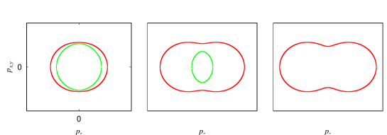
Figure 1: Modification of the Fermi sea as $U_{A}$ is increased from left to right. The larger Fermi sea ($F^{-}$) takes a prolate shape, while the smaller one ($F^{+}$) an oblate shape for a given $U_{A}$. In the large $U_{A}$ limit (completely polarized case), $F^{+}$ disappears as in the right panel.

The mean spin polarization is then given by

$${\bar{s}_{z}}=\frac{1}{2}\langle\Sigma_{z}\rangle = -i\int_{C}\frac{d^{4}p}{(2\pi)^{4}}{\rm tr}[\gamma_{5}\gamma_{3}G_{A}(p)]$$ (18)

$$= {\frac{1}{2}\left[\int_{F^{+}}\frac{d^{3}p}{(2\pi)^{3}}\frac{U_{A}+\beta}{\epsilon_{+}}+\int_{F^{-}}\frac{d^{3}p}{(2\pi)^{3}}\frac{U_{A}-\beta}{\epsilon_{-}}\right]}$$ (19)

with $\beta=\sqrt{p_{z}^{2}+m^{2}}$, from which we can immediately see the non-vanishing value of $U_{A}$ gives rise to spin polarization. Since the spin polarization is not necessarily measurable quantity, we’d better to see another observable, the magnetization, which is defined as the magnetic moment per unit volume and the magnetic field directly couples with it. In QED the magnetic field couples with quarks by way of the term, $\mu_{q}{\bar{q}}\sigma_{\mu\nu}qF^{\mu\nu}$, with the Dirac magnetic moment $\mu_{q}=e/(2m)$, and we can easily see that the magnetization ${\bf M}$ is directed to the $z$ direction;

$$M_{3} = -i\int_{C}\frac{d^{4}p}{(2\pi)^{4}}{\rm tr}[\gamma_{0}\gamma_{5}\gamma_{3}G_{A}(p)]$$ (20)

$$= {\frac{1}{2}\left[-\int_{F^{+}}\frac{d^{3}p}{(2\pi)^{3}}\frac{m}{\beta}+\int_{F^{-}}\frac{d^{3}p}{(2\pi)^{3}}\frac{m}{\beta}\right]}$$ (21)

with $\beta=\sqrt{p_{z}^{2}+m^{2}}$ in the units of the Dirac magnetic moment. Note that the magnetization of each Fermi sea has now the opposite direction and it does not explicitly depend on $U_{A}$, but the net magnetization arises by way of the exchange splitting of the Fermi sea. Thus we see the ground state holds ferromagnetism in the presence of $U_{A}$.

3 Color magnetic superconductivity

If FM is realized in quark matter, it might be in the CSC phase. In this section we discuss a possibility of the coexistence of FM and CSC, which we call Color magnetic superconductivity [15].

In passing, it would be worth mentioning the corresponding situation in condensed matter physics. Magnetism and superconductivity (SC) have been two major concepts in condensed matter physics and their interplay has been repeatedly discussed [16]. Very recently some materials have been observed to exhibit the coexistence phase of FM and SC, which properties have not been fully understood yet; itinerant electrons are responsible to both phenomena in these materials and one of the important features is both phases cease at the same critical pressure [17]. In our case we shall see somewhat different features, but the similar aspects as well.

We begin with an OGE-type action:

$$I_{int}=-g^{2}\frac{1}{2}\int{\rm d^{4}}x\int{\rm d^{4}}y\left[\bar{\psi}(x)\gamma^{\mu}\frac{\lambda_{a}}{2}\psi(x)\right]D_{\mu\nu}(x,y)\left[\bar{\psi}(y)\gamma^{\nu}\frac{\lambda_{a}}{2}\psi(y)\right],$$ (22)

where $D^{\mu\nu}$ denotes the gluon propagator. By way of the mean-field approximation, we have

$$I_{MF}=\frac{1}{2}\int\frac{{\rm d}^{4}p}{(2\pi)^{4}}\left(\begin{array}[]{l}\bar{\psi}(p)\\ \bar{\psi}_{c}(p)\\ \end{array}\right)^{T}G^{-1}(p)\left(\begin{array}[]{l}\psi(p)\\ \psi_{c}(p)\\ \end{array}\right)\\$$ (23)

in the Nambu-Gorkov formalism. The inverse quark Green function $G^{-1}(p)$ involves various self-energy (mean-field) terms, of which we only keep the color singlet particle-hole $V(p)$ and color $\bar{3}$ particle-particle ($\Delta$) mean-fields; the former is responsible to ferromagnetism, while the latter to superconductivity,

$$G^{-1}(p) = \left(\begin{array}[]{cc}/{\!\!\!}{p}-m+/{\!\!\!}{\mu}+V(p)&\gamma_{0}\Delta^{\dagger}(p)\gamma_{0}\\ \Delta(p)&/{\!\!\!}{p}-m-/{\!\!\!}{\mu}+\overline{V}(p)\\ \end{array}\right),$$ (26)

$$= \left(\begin{array}[]{cc}G_{11}(p)&G_{12}(p)\\ G_{21}(p)&G_{22}(p)\\ \end{array}\right)^{-1}$$ (29)

where

$$\psi_{c}(k)=C\bar{\psi}^{T}(-k),~{}~{}~{}\overline{V}\equiv CV^{T}C^{-1}.$$ (30)

Taking into account the lowest diagram, we can then write down the self-consistent equations for the mean-fields, $V$ and $\Delta$:

$$-V(k)=(-ig)^{2}\int\frac{{\rm d}^{4}p}{i(2\pi)^{4}}\{-iD^{\mu\nu}(k-p)\}\gamma_{\mu}\frac{\lambda_{\alpha}}{2}\{-iG_{11}(p)\}\gamma_{\nu}\frac{\lambda_{\alpha}}{2}.$$ (31)

and

$$-\Delta(k)=(-ig)^{2}\int\frac{{\rm d}^{4}p}{i(2\pi)^{4}}\{-iD^{\mu\nu}(k-p)\}\gamma_{\mu}\frac{-(\lambda_{\alpha})^{T}}{2}\{-iG_{21}(p)\}\gamma_{\nu}\frac{\lambda_{\alpha}}{2}.$$ (32)

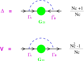
Figure 2: Graphical interpretations of the coupled equations (31) and (32) with coefficients in front of R.H.S. given by $N_{c}$.

Applying the Fierz transformation for the Fock exchange energy term (31) we can see that there appear the color-singlet scalar, pseudoscalar, vector and axial-vector self-energies. In general we must take into account these self-energies in $V$, $V=U_{s}+\gamma_{5}U_{ps}+\gamma_{\mu}U_{v}^{\mu}+\gamma_{\mu}\gamma_{5}U_{av}^{\mu}$ with the mean-fields $U_{i}$. Here we retain only $U_{s},U_{v}^{0},U_{av}^{3}$ in $V$ and suppose that others to be vanished. We shall see this ansatz gives self-consistent solutions for Eq.(31) because of axial and reflection symmetries of the Fermi seas under the zero-range approximation for the gluon propagator. We furthermore discard the scalar mean-field $U_{s}$ and the time component of the vector mean-field $U_{v}^{0}$ for simplicity since they are irrelevant for the spin degree of freedom.

According to the above assumptions and considerations the mean-field $V$ in Eq.(29) renders

$$V=\gamma_{3}\gamma_{5}U_{A},~{}~{}~{}U_{A}\equiv U_{av}^{3},$$ (33)

with VA $U_{A}$. Then the diagonal component of the Green function $G_{11}(p)$ is written as

$$G_{11}(p)=\left[G_{A}^{-1}-\gamma_{0}\Delta^{\dagger}\gamma_{0}\tilde{G}_{A}\Delta\right]^{-1}$$ (34)

with

$$G_{A}^{-1}(p) = /{\!\!\!}{p}-m+/{\!\!\!}{\mu}-\gamma_{5}\gamma_{3}U_{A},$$ (35)

$$\tilde{G}_{A}^{-1}(p) = /{\!\!\!}{p}-m-/{\!\!\!}{\mu}-\overline{\gamma_{5}\gamma_{3}}U_{A},$$ (36)

where $\overline{\gamma_{5}\gamma_{3}}=\gamma_{5}\gamma_{3}$ and $G_{A}(p)$ is the Green function with $U_{A}$ which is determined self-consistently by way of Eq. (31).

Before constructing the gap function $\Delta$, we first find the single-particle spectrum and their eigenspinors in the absence of $\Delta$, which is achieved by diagonalization of the operator $G_{A}^{-1}$. We have already known four single-particle energies $\epsilon_{\pm}$ (positive energies) and $-\epsilon_{\pm}$ (negative energies), which are given as

$$\epsilon_{\pm}({\mbox{\boldmath$p$}})=\sqrt{{\mbox{\boldmath$p$}}^{2}+U_{A}^{2}+m^{2}\pm 2U_{A}\sqrt{m^{2}+p_{z}^{2}}},$$ (37)

and the eigenspinors $\phi_{s},~{}s=\pm$ should satisfy the equation, $G_{A}^{-1}(\epsilon_{s},{\bf p})\phi_{s}=0$.

Here we take the following ansatz for $\Delta$:

$$\Delta({\mbox{\boldmath$p$}}) = \sum_{s=\pm}\tilde{\Delta}_{s}({\mbox{\boldmath$p$}})B_{s}({\mbox{\boldmath$p$}}),$$

$$B_{s}({\mbox{\boldmath$p$}}) = \gamma_{0}\phi_{-s}({\mbox{\boldmath$p$}})\phi_{s}^{\dagger}({\mbox{\boldmath$p$}}).$$ (38)

The structure of the gap function (38) is then inspired by a physical consideration of a quark pair as in the usual BCS theory: we consider here the quark pair on each Fermi surface with opposite momenta, ${\bf p}$ and $-{\bf p}$ so that they result in a linear combination of $J^{\pi}=0^{-},1^{-}$ (see Fig. 3).

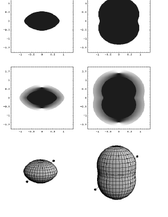
Figure 3: Deformed Fermi seas and the quark pair on each surface. The top figures show those in the absence of $\Delta_{\pm}$ and the middle figures diffusion of the Fermi surfaces in the presence of $\Delta_{\pm}$. The bottom ones show the quark pairing on the Fermi surfaces.

Figure 4: Schematic view of the polar-angle dependence of the gap functions at the Fermi surface, (a) for $m=0$ and (b) for $m\neq 0$.

$\tilde{\Delta}_{s}$ is still a matrix in the color-flavor space. Since the antisymmetric nature of the fermion self-energy imposes a constraint on the gap function [1],

$$C\Delta({\mbox{\boldmath$p$}})C^{-1}=\Delta^{T}({-\mbox{\boldmath$p$}}).$$ (39)

$\tilde{\Delta}_{n}({\mbox{\boldmath$p$}})$ must be a symmetric matrix in the spaces of internal degrees of freedom. Taking into account the property that the most attractive channel of the OGE interaction is the color antisymmetric ${\bar{3}}$ state, it must be in the flavor singlet state.

Thus we can choose the form of the gap function as

$$\left(\tilde{\Delta}_{s}\right)_{\alpha\beta;ij}=\epsilon^{\alpha\beta 3}\epsilon^{ij}\Delta_{s}$$ (40)

for the two-flavor case (2SC), where $\alpha,\beta$ denote the color indices and $i,j$ the flavor indices. Then the quasi-particle spectrum can be obtained by looking for poles of the diagonal Green function, $G_{11}$:

$$E_{s}({\mbox{\boldmath$p$}}) =\left\{\begin{array}[]{ll}\sqrt{(\epsilon_{s}({\mbox{\boldmath$p$}})-\mu)^{2}+|\Delta_{s}({\mbox{\boldmath$p$}})|^{2}}&\mbox{for color 1, 2}\\ \sqrt{(\epsilon_{s}({\mbox{\boldmath$p$}})-\mu)^{2}}&\mbox{for color 3}\end{array}\right.$$ (43)

Note that the quasi-particle energy is independent of color and flavor in this case, since we have assumed a singlet pair in flavor and color.

Gathering all these stuffs to put them in the self-consistent equations, we have the coupled gap equations for $\Delta_{s}$,

$$\Delta_{s^{\prime}}(k,\theta_{k})\!=\!\frac{N_{c}\!+\!1}{2N_{c}}\tilde{g}^{2}\!\!\int\!\!\frac{{\rm d}p\,{\rm d}\theta_{p}}{(2\pi)^{2}}p^{2}\sin\theta_{p}\!\!\sum_{s}T_{s^{\prime}s}(k,\theta_{k},p,\theta_{p})\frac{\Delta_{s}(p,\theta_{p})}{2E_{s}(p,\theta_{p})},$$ (44)

and the equation for $U_{A}$,

$$U_{A}=-\frac{N_{c}^{2}-1}{4N_{c}^{2}}\tilde{g}^{2}\int\frac{{\rm d}^{3}p}{(2\pi)^{3}}\sum_{s}\left\{\theta(\mu-\epsilon_{s}(\mbox{\boldmath$p$}))+2v_{s}^{2}({\mbox{\boldmath$p$}})\right\}\frac{U_{A}+s\beta_{p}}{\epsilon_{s}(\mbox{\boldmath$p$})},$$ (45)

within the “contact” interaction, $\tilde{g}^{2}\equiv g^{2}/\Lambda^{2}$, (see Eq. (47)), where $v_{s}^{2}(\mbox{\boldmath$p$})$ denotes the momentum distribution of the quasi-particles. We find that the expression for $U_{A}$, Eq. (45), is nothing but the simple sum of the expectation value of the spin operator with the weight of the occupation probability of the quasi-particles $v_{s}^{2}$ for two colors and the step function for remaining one color (cf. (19)).

Carefully analyzing the structure of the function $T_{s^{\prime}s}$ in Eq. (44), we can easily find that the gap function $\Delta_{s}$ should have the polar angle ($\theta$) dependence on the Fermi surface,

$$\Delta_{s}(p^{F}_{s},\theta)=\frac{p^{F}_{s}(\theta)\sin\theta}{\mu}\left(-s\frac{m}{\sqrt{m^{2}+(p^{F}_{s}(\theta)\cos\theta)^{2}}}R+F\right),$$ (46)

with constants $F$ and $R$ to be determined (see Fig. 4).

As a characteristic feature, both the gap functions have nodes at poles ($\theta=0,\pi$) and take the maximal values at the vicinity of equator ($\theta=\pi/2$), keeping the relation, $\Delta_{-}\geq\Delta_{+}$. This feature is very similar to ${}^{3}P$ pairing in liquid ³He or nuclear matter [19, 20]; actually we can see our pairing function Eq. (46) to exhibit an effective $P$ wave nature by a genuine relativistic effect by the Dirac spinors. Accordingly the quasi-particle distribution is diffused (see Fig. 3)

Self-consistent solutions

Here we demonstrate some numerical results; we replaced the original OGE by the “contact” interaction with the cutoff around the Fermi surface in the momentum space,

$$D^{\mu\nu}\rightarrow-g^{\mu\nu}/\Lambda^{2},~{}~{}~{}\Delta_{s}({\bf p})\rightarrow\Delta_{s}({\bf p})\theta(\delta-|\epsilon_{s}-\mu|)$$ (47)

as in the BCS theory in the weak-coupling limit [21].

First we show the magnitude of $U_{A}$ (Fig. 5). It is seen that the axial-vector mean-field (spin polarization) appears above a critical density and becomes larger as baryon number density gets higher. Moreover, the results for different values of the quark mass show that spin polarization grows more for the larger quark mass. This is because a large quark mass gives rise to much difference in the Fermi seas of two different “spin” states, which leads to growth of the exchange energy in the axial-vector channel. A slight reduction of $U_{A}$ arises as a result of diffuseness of the Fermi surface due to $\Delta_{s}$. As seen in Eq. (45), $U_{A}$ can be obtained as addition and cancellation of the contributions by two different Fermi seas; the latter term is more momentum dependent than the former one and thereby $v_{s}^{2}({\bf p})$ enhances the cancellation term (see Fig. 3).

Figure 5: Axial-vector mean-field (VA) as a function of baryon number density $\rho_{B}$($\rho_{0}=0.16$fm^-3). Solid (dashed) lines denote VA in the presence (absence) of CSC.

Figure 6: Mean values of the gap functions, $\Delta_{\pm}$ and their mass dependence.

Next we show the gap function as a function of $\rho_{B}$ (Fig. 6). To see the bulk behavior of the gap function, we use the mean-value with respect to the polar angle on the Fermi surface,

$$\langle\Delta_{\pm}\rangle\equiv\left(\int_{0}^{\pi}{\rm d}\theta\frac{\sin\theta}{2}\Delta_{\pm}^{2}\right)^{1/2}.$$ (48)

The mean values $\langle\Delta_{\pm}\rangle$ begin to split with each other at a density where $U_{A}$ becomes finite. We’d like to make a comment here. One may be surprised to see their value of $O({\rm GeV})$, coming from our parameter choice. However, what we’d like to reveal here is not their realistic values but a possibility of color magnetic superconductivity and its qualitative features. More realistic study, of course, is needed by carefully checking our approximations, especially the contact interaction and the sharp cutoff at the Fermi surface.

With these figures we can say that FM and CSC barely interfere with each other.

4 Chiral symmetry and magnetism

We have seen that the quark mass dependence of ferromagnetism should be important, while we have treated it as an input parameter. When we consider the realization of chiral symmetry in QCD, the quark mass should be dynamically generated as a result of the vacuum “superconductivity”; $q\bar{q}$ pairs are condensed in the vacuum. We consider here $SU(2)_{L}\times SU(2)_{R}$ symmetry. Then Lagrangian should be globally invariant under the operation of any group element with constant parameters, except the symmetry-breaking term stemming from the small current mass, $m_{c}$. Here we’d like to suggest another mechanism leading to FM in quark matter with recourse to chiral symmetry. We shall see that FM may be realized without accompanying spin polarization.

Consider the following parameterization for the combination of the quark bilinear fields by introducing the auxiliary fields, $\rho$ and $\theta_{i}$:

$$\bar{\psi}\psi+i\gamma_{5}\mbox{\boldmath$\tau$}\bar{\psi}i\gamma_{5}\mbox{\boldmath$\tau$}\psi=\rho\exp(i\gamma_{5}\mbox{\boldmath$\tau$}\cdot\mbox{\boldmath$\theta$}).$$ (49)

Then it resides on the chiral “circle” with “modulus ”$\rho$ and “ phase”$\theta_{i}$, any point on which is equivalent with each other in the chiral limit, $m_{c}=0$, and moved to another point by a chiral transformation. We conventionally choose a definite point, $\langle{\rm vac}|\rho|{\rm vac}\rangle=f_{\pi}$ ($f_{\pi}$: the pion decay constant) and $\langle{\rm vac}|\theta_{i}|{\rm vac}\rangle=0$, for the vacuum, which is flavor singlet and parity eigenstate. In the following we shall see that the phase degree of freedom is related to spin polarization; that is, the “phase condensation” with a non-vanishing value of $\theta_{i}$ leads to FM [22].

Separating the fields $\rho$ and $\theta_{i}$ into the classical ones and fluctuations around them, and discarding any fluctuation the mean-field theory proceeds:

$$\rho\rightarrow\langle\rho\rangle[\geq 0],~{}~{}~{}\theta_{i}\rightarrow\langle\theta_{i}\rangle.$$ (50)

Assuming the simplest but nontrivial form of the classical chiral angle such that $\theta_{3}({\bf r})={\bf q\cdot r},\theta_{1,2}=0$, we call this set a dual chiral density wave (DCDW) :

$$\langle\bar{\psi}\psi\rangle = \Delta\cos{\bf q\cdot r}$$

$$\langle\bar{\psi}i\gamma_{5}\tau_{3}\psi\rangle = \Delta\sin{\bf q\cdot r}.$$ (51)

It should be obvious that if $\Delta$ vanishes, the phase degree of freedom has to become redundant, as seen later. It would be worth mentioning that similar configuration has been studied in other contexts [23, 24, 25]. Note that the configuration in (51) breaks rotational invariance as well as translational invariance, but the latter invarianvce is recovered by an isospin rotation [28].

Taking the Nambu-Jona-Lasinio (NJL) model as a simple but nontrivial model [29], we explicitly demonstrate that quark matter becomes unstable for a formation of DCDW above a critical density; the NJL model has been originally presented to demonstrate a realization of chiral symmetry in the vacuum, while recently it been also used as an effective model embodying spontaneous breaking of chiral symmetry in terms of quark degree of freedom [30]

$$L_{NJL}=\bar{\psi}(i\partial/-m_{c})\psi+G[(\bar{\psi}\psi)^{2}+(\bar{\psi}i\gamma_{5}\mbox{\boldmath$\tau$}\psi)^{2}]$$ (52)

Using the mean-field approximation (MFA) with the DCDW configuration, we introduce a new quark field $\psi_{W}$ by the Weinberg transformation [31],

$$\psi_{W}=\exp[i\gamma_{5}\tau_{3}{\bf q\cdot r}/2]\psi,$$ (53)

to get the transformed Lagrangian,

$${\cal L}_{MF}=\bar{\psi}_{W}[i\partial/-M-1/2\gamma_{5}\tau_{3}q/]\psi_{W}-G\Delta^{2},$$ (54)

with the dynamically generated mass, $M\equiv-2G\Delta$ and $q^{\mu}=(0,{\bf q})$. This procedure embodies translational invariance of the ground state, and shows that we essentially consider a “uniform” problem, while we introduced the space-dependent mean-fields at the beginning. We briefly summarize in Table 3 the relation of the transformed frame to the original one. Note that the transformed Lagrangian becomes the same as the familiar form used in discussions of chiral symmetry realization within the NJL model, except the isovector and axial-vector coupling term $\gamma_{5}\tau_{3}q/$. We can see the role of the wave vector $\bf q$ is the same as AV introduced in the previous sections.

Table 3: Diagram of the Weinberg transformation.

$\langle\bar{\psi}\psi\rangle\neq 0$	$\Longleftrightarrow$	$\langle\bar{\psi}_{W}\psi_{W}\rangle=\Delta(\neq 0)$
$\langle\bar{\psi}i\gamma_{5}\tau_{3}\psi\rangle\neq 0$		$\langle\bar{\psi}_{W}i\gamma_{5}\tau_{3}\psi_{W}\rangle=0$
		$q/2\propto\nabla\theta$   (“AV”)
non-uniform		uniform

The Dirac equation for $\psi_{W}$ then renders

$$\left(i\partial/-M-1/2\tau_{3}\gamma_{5}q/\right)\psi_{W}=0.$$ (55)

We can find a spatially uniform solution for the quark wave function, $\psi_{W}=u_{W}(p)\exp(i{\bf p\cdot r})$, and the energy eigenvalue is given as

$$E_{p}^{\pm}=\sqrt{E_{p}^{2}+|{\bf q}|^{2}/4\pm\sqrt{({\bf p}\cdot{\bf q})^{2}+M^{2}|{\bf q}|^{2}}},~{}~{}~{}E_{p}=(M^{2}+|{\bf p}|^{2})^{1/2}$$ (56)

for positive energy (valence) quarks with different polarizations. For negative energy quarks in the Dirac sea, they have a spectrum symmetric with respect to null line because of charge conjugation symmetry in the Lagrangian (54). The single-particle spectrum (56) shows again an analogous feature to the exchange splitting between two eigenenergies with different polarizations in the presence of ${\bf q}$; hereafter, we choose ${\bf q}//\hat{z}$, ${\bf q}=(0,0,q),~{}q\geq 0$, without loss of generality.

Thus each flavor quark shows the same energy spectrum (56) even in the presence of the isospin dependent AV and its form is the same as in Eq. (14). However, there is one and important difference from the previous sections; we have considered the flavor singlet AV, while we are now considering the isovector AV here. The eigenspinor $u_{W,i}^{\pm},~{}i=u,d$ for each flavor satisfies the same Dirac equation for a given energy eigenvalue, except the different sign in the AV term, so that we have the different form for each flavor; $u_{W,u}^{\pm}=u_{W,d}^{\mp}$. The mean-value of the spin operator $\Sigma_{z}=\left(\begin{array}[]{cc}\sigma_{3}&0\\ 0&\sigma_{3}\end{array}\right)$ is then given by

$$\bar{s}_{z,u}^{\pm}=\frac{1}{2}u^{\pm\dagger}_{W,u}\Sigma_{z}u_{W,u}^{\pm}=\frac{1}{2}\frac{q/2\pm\beta}{E^{\pm}_{p}},$$ (57)

with $\beta=\sqrt{p_{z}^{2}+M^{2}}$ for $u$ quarks. The corresponding value for $d$ quarks is also given as $\bar{s}_{z,d}^{\pm}=-\bar{s}_{z,u}^{\pm}$. Thus we can see two flavors are oppositely polarized to each other. Since the integral of $\bar{s}_{z,i}^{\pm}$ over the Fermi seas should be finite for $q\neq 0$ for each flavor, the spin polarization of each flavor is finite but has opposite direction to each other. Consequently the total spin polarization or the flavor singlet AV is always vanished in this case. However, note that this result is never conflicted with FM of quark matter by considering the magnetization. As we have already noted, the response of the system to the magnetic field goes through the magnetization. Taking into account the difference of electric charges of two flavors $Q_{i}$, $Q_{u}=+2/3e$ and $Q_{d}=-1/3e$, we can see that each flavor coherently contributes to the magnetization, instead.

Thermodynamic potential

The thermodynamic potential is given as

$$\Omega_{\rm total} = \gamma\sum_{s=\pm}\int\frac{d^{3}p}{(2\pi)^{3}}(E^{s}_{p}-\mu)\theta_{s}-\gamma\sum_{s=\pm}\int\frac{d^{3}p}{(2\pi)^{3}}E^{s}_{p}+M^{2}/4G$$ (58)

$$\equiv \Omega_{\rm val}+\Omega_{\rm vac}+M^{2}/4G.$$

where $\theta_{\pm}=\theta(\mu-E^{\pm}_{p})$, $\mu$ the chemical potential and $\gamma$ is the degeneracy factor $\gamma=N_{f}N_{c}$. The first term $\Omega_{\rm val}$ is the contribution by the valence quarks filled up to the chemical potential, while the second term $\Omega_{\rm vac}$ is the vacuum contribution that is formally divergent. We shall see both contributions are indispensable in our discussion. Once $\Omega_{\rm total}$ is properly evaluated, the equations to be solved to determine the optimal values of $\Delta$ and $q$ are

$$\frac{\partial\Omega_{\rm total}}{\partial\Delta}=\frac{\partial\Omega_{\rm total}}{\partial q}=0.$$ (59)

Since the NJL model is not renormalizable, we need some regularization procedure to get a meaningful finite value for the vacuum contribution. Consider the sum of the negative energy over the Dirac sea,

$$\Omega_{\rm{vac}}=-\gamma\sum_{s=\pm}\int\frac{d^{3}p}{(2\pi)^{3}}E^{s}_{p}-\Omega_{\rm ref},$$ (60)

where we subtracted an irrelevant constant $\Omega_{\rm ref}=-2\gamma\int\frac{d^{3}p}{(2\pi)^{3}}E_{p}$ with an arbitrary reference mass $M=M_{\rm ref}$ to make the following procedure mathematically well-defined. Since the energy spectrum is no more rotation symmetric, we cannot apply the usual momentum cut-off regularization (MCOR) scheme to regularize $\Omega_{\rm{vac}}$. Instead, we adopt the proper-time regularization (PTR) scheme [32]. We think this is a most suitable one for our purpose, since $\Omega_{\rm{vac}}$ counts the spectrum change under the “external” axial-vector field. It has been shown that the vacuum polarization effect under the external electromagnetic field can be treated in a gauge invariant way, where the energy spectrum is also deformed depending on the field strength [32]. It is also known that the consequences from the NJL model are almost regularization-scheme independent [30], including the PTR scheme.

Introducing the proper-time variable $\tau$, we eventually find

$$\Omega_{\rm vac}\!=\!\frac{\gamma}{8\pi^{3/2}}\int_{0}^{\infty}\!\!\frac{d\tau}{\tau^{5/2}}\int^{\infty}_{-\infty}\!\!\frac{dp_{z}}{2\pi}\!\left[e^{-(\sqrt{p_{z}^{2}\!+\!M^{2}}+q/2)^{2}\tau}\!+\!e^{-(\sqrt{p_{z}^{2}+M^{2}}\!-\!q/2)^{2}\tau}\right],$$ (61)

except an irrelevant constant $\Omega_{\rm ref}$, which is reduced to the standard formula [30] in the limit $q\rightarrow 0$.

We can easily see, from Eq. (61), that the $q$ degree of freedom becomes superfluous and theory must become trivial in the limit $m\rightarrow 0$, which is equivalent to $\Delta\rightarrow 0$ in the chiral limit: all the observables must be independent of $q$. This salient feature is consistent with the form of DCDW. The integral with respect to the proper time $\tau$ is not well defined as it is, since it is still divergent due to the $\tau\sim 0$ contribution. Regularization proceeds by replacing the lower bound of the integration range by $1/\Lambda^{2}$, which corresponds to the momentum cut-off in the MCOR scheme.

For given chemical potential $\mu$, and $M$ and $q$ we can evaluate the valence contribution $\Omega_{\rm val}$ using Eq. (56) and write down the general formula analytically. Then the thermodynamic potential can be expressed as $\Omega_{\rm val}=\epsilon_{\rm val}(q)-\mu\rho_{\rm val}(q),$ where $\epsilon_{\rm val}(q)$ and $\rho_{\rm val}(q)$ are the energy density and the quark-number density, respectively. They consist of two terms corresponding to the two Fermi seas with different polarizations: $\epsilon_{\rm val}(q)=\epsilon^{-}(q)+\epsilon^{+}(q)$ and $\rho_{\rm val}(q)=\rho_{\rm val}^{-}(q)+\rho_{\rm val}^{+}(q)$. We present some examples about the instability of the usual NJL ground state with respect to spontaneous generation of DCDW. In the present calculation chiral symmetry restoration occurs at the first order in the case without DCDW. We can see the NJL ground state becomes unstable at the critical chemical potential $\mu_{c1}$, and symmetry restoration is delayed until $\mu_{c2}$ by the presence of DCDW. This dragging effect by DCDW is one of the important features.

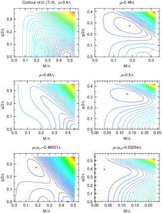
Figure 7: Countour map of the thermodynamic potential in the dynamical mass ($M$) - wave number ($q$) plane. The absolute minimum is denoted by the cross for given density. We have the first order phase transitions in this calculation.

Figure 8: Density dependence of $M$ and $q$, compared with the usual result with $q=0$. There appear two critical chemical potentials; the lower one indicates the instability of the ground state for formation of DCDW, while the higher one restoration of chiral symmetry.

5 Summary and Concluding remarks

In this talk we have discussed a magnetic aspect of quark matter based on QCD. First, we have introduced “ferromagnetism” (FM) in QCD, where the Fock exchange interaction plays an important role. Presence of the axial-vector mean-field (AV) after the Fierz transformation is essential to give rise to FM, in the context of self-consistent framework. As one of the features of the relativistic FM, we have seen that the Fermi sea is deformed in the presence of AV; the Fermi sea has a prolate shape for the majority spin particles, while an oblate shape for the minority spin particles.

We have then discussed a possibility of color magnetic superconductivity and seen coexistence of FM and CSC is possible. Our ansatz for quark pairing shows an effective $P$- wave pair condensation and gives a polar angle dependence of the gap function, which looks similar to liquid ³He A - phase. Note that this ansatz is never unique for color magnetic superconductivity and other types may be also possible [18], where the gap function should show other angle dependence. In this context recent studies about $S=1$ quark pairing may be interesting [33].

We have briefly discussed a relation of magnetism to chiral symmetry and presented an idea, dual chiral density wave (DCDW), which should lead to FM. Using, e.g., the NJL model we have demonstrated under what conditions the ground state becomes unstable for formation of DCDW. We have found the usual ground state becomes surely unstable at the critical density and stays in FM between the first and the second critical densities.

The FM induced by DCDW has many interesting features different from the Bloch mechanism. Unfortunately we have not revealed them yet, but it would be interesting to examine whether DCDW is possible in the CSC phase.

The symmetry breaking pattern is summarized as follows: in the condensation of the flavor singlet AV, it violates rotation symmetry,

$$O(3)\rightarrow O(2),$$ (62)

while the DCDW state does flavor symmetry as well as rotation symmetry,

$$O(3)\times SU(2)_{V}\rightarrow O(2)\times U_{I_{3}}(1).$$ (63)

The latter situation is similar to the neutral pion condensation in nuclear matter.

It would be important to figure out the low energy excitation modes (Nambu-Goldstone modes) built on the ferromagnetic phase. The spin waves are well known in the Heisenberg model [12]. Then , how about our case [34]?

If quark matter is in the ferromagnetic phase, it may produce the dipolar magnetic field by their magnetic moment. Since the total magnetic dipole moment $M_{q}$ should be simply given as $M_{q}=\mu_{q}\cdot(4\pi/3\cdot r_{q}^{3})n_{q}$ for the quark sphere with the quark core radius $r_{q}$ and the quark number density $n_{q}$. Then the dipolar magnetic field at the star surface $R$ takes the maximal strength at the poles,

$$B_{\rm max}=\frac{8\pi}{3}\left(\frac{r_{q}}{R}\right)^{3}\mu_{q}n_{q}=10^{15}[{\rm G}]\left(\frac{r_{q}}{R}\right)^{3}\left(\frac{\mu_{q}}{\mu_{N}}\right)\left(\frac{n_{q}}{0.1{\rm fm}^{-3}}\right).$$ (64)

We have not considered the electromagnetic interaction between quarks and the induced magnetic field. It would be interesting to see how the situation changes when we take it into account; symmetry restoration [35] or mixing between magnetic field and gluon field are among them [36].

Finally we’d like to give a comment about fluctuations. In this talk we have completely discarded fluctuations and been only concerned with the mean-field. It would be reasonable to study the phase transition, at least qualitatively. However, we know some fluctuations or correlations between relevant operators should have some effects even before the phase transitions. In particular the axial and magnetic susceptibilities in normal quark matter would be interesting; they might have important consequence,e.g., for quark-quark pairing correlation as in ³He superfluidity [19].

1

References

- [1] B. C. Barrois, Nucl. Phys. B129 (1977) 390,
- [2] D. Bailin and A. Love, Phys. Rept. 107 (1984) 325.
- [3] For recent reviews of CSC, K. Rajagopal and F. Wilczek, hep-ph/0011333; M. Alford, Ann. Rev. Nucl. Part. Sci. 51 (2001) 131, and referenses cited therein.
- [4] For a review, G. Chanmugam, Annu. Rev. Astron. Astrophys. 30 (1992) 143.
- [5] B. Paczyński, Acta. Astron. 41 (1992) 145; R.C.Duncan and C. Thompson, Astrophys. J. 392 (1992) L19; C. Thompson and R.C.Duncan, Mon. Not. R. Astron. Soc. 275 (1995) 255.
- [6] C. Kouveliotou et al., Nature 393 (1998) 235; K. Hurley et al., Astrophys. J. 510 (1999) L111.
- [7] S.B. Popov, in this proceedings.
-
[8]
V.L. Ginzburg, Sov. Phys. Dokl. 9 (1964) 329;
L. Woltjer, Ap. J. 140 (1964) 1309. - [9] V.R. Pandharipande, V.K. Garde and J.K. Srivastava, Phys. Lett. B38 485.
- [10] T. Tatsumi, Phys. Lett. B489 (2000) 280.
- [11] F. Bloch, Z. Phys. 57 (1929) 545.
- [12] e.g. K.Yoshida, Theory of Magnetism (Springer-Verlag Berlin Heidelberg, 1996).
- [13] T. Maruyama and T. Tatsumi, Nucl. Phys. A693 (2001) 710.
- [14] H.Müther and A.Sedrakian, Phys.Rev.Lett. 88 (2002) 252503; Phys.Rev. D67 (2003) 085024.
- [15] E. Nakano, T. Maruyama and T. Tatsumi, Phys. Rev. D68 (2003) 105001.
- [16] L.N. Buaevskii et al., Adv. Phys. 34 (1985) 175.
- [17] S.S. Sexena et al., Nature 406 (2000) 587; C.Pfleiderer et al., Nature 412 (2001) 58; N.I.Karchev et al., Phys. Rev. Lett. 86 (2001) 846; K.Machida and T.Ohmi, Phys. Rev. Lett. 86 (2001) 850
- [18] K. Nawa, E. Nakano, T. Maruyama and T. Tatsumi, in progress.
- [19] A. J. Leggett, Rev. Mod. Phys. 47 (1975) 331.
- [20] R. Tamagaki, Prog. Theor. Phys. 44 (1970) 905; M. Hoffberg, A.E. Glassgold, R.W. Richardson and M. Ruderman, Phys. Rev. Lett. 24 (1970) 775.
- [21] R.D. Pisarski and D.H. Rischke, Phys. Rev. D60 (1999) 094013.
- [22] T. Tatsumi and E. Nakano, in preparation.
- [23] F. Dautry and E.M. Nyman, Nucl. Phys. 319 (1979) 323.
- [24] M. Kutschera, W. Broniowski and A. Kotlorz, Nucl. Phys. A516 (1990) 566.
- [25] K. Takahashi and T. Tatsumi, Phys. Rev. C63 (2000) 015205; Prog. Theor. Phys. 105 (2001) 437.
-
[26]
D.V. Deryagin, D. Yu. Grigoriev and V.A. Rubakov, Int. J. Mod. Phys. A7
(1992) 659.
B.-Y. Park, M.Rho, A.Wirzba and I.Zahed, Phys. Rev. D62 (2000) 034015.
R. Rapp, E.Shuryak and I. Zahed, Ohys. Rev. D63 (2001) 034008. - [27] A.W. Overhauser, Phys. Rev. 128 (1962) 1437.
- [28] D.K. Campbell, R.F. Dashen and J.T. Manassah, Phys. Rev. D12 (1975) 979;1010.
- [29] Y. Nambu and G. Jona-Lasinio, Phys. Rev. 122 (1961) 345; 124 (1961) 246.
-
[30]
S.P. Klevansky, Rev. Mod. Phys. 64 (1992) 649.
T. Hatsuda and T. Kunihiro, Phys. Rep. 247 (1994) 221. - [31] S. Weinberg, The quantum theory of field II(Cambridge, 1996).
- [32] J. Schwinger, Phys. Rev. 92 (1951) 664.
-
[33]
M.G. Alford, J.A. Bowers, J.M. Cheyne and G.A. Cowan, hep-ph/0210106.
M. Buballa, J. Hos̃ek and M. Oertel, hep-ph/0204275. - [34] F. Sannino, in this proceedings.
-
[35]
S.P. Klevansky and R.H. Lemmer, Phys. Rev. D39
(1989) 3478.
H. Suganuma and T. Tatsumi, Ann. Phys. 208 (1991) 470. - [36] M. Alford,K. Rajagopal and F. Wilczek, Phys. Lett. B422 (1998) 247; M. Alford, J. Berges and K. Rajagopal, Nucl. Phys. B571 (2000) 269.