Neutrino Oscillations, Fluctuations and Solar Magneto-gravity Waves

Abstract:

This review has two parts. The first part summarizes the current observational constraints on fluctuations in the solar medium deep within the solar Radiative Zone, and shows how the KamLAND and SNO-salt data combine to make the experimental determination of the neutrino oscillation parameters largely insensitive to prior assumptions about the nature of these oscillations. As part of a search for plausible sources of solar fluctuations to which neutrinos could be sensitive, the second part of the talk summarizes a preliminary analysis of the influence of magnetic fields on helioseismic waves. Using simplifying assumptions which should apply to modes in the solar radiative zone, we find a resonance between Alfvén waves and helioseismic $g$-modes which potentially modifies the solar density profile fairly significantly over comparatively short distance scales, too narrow to be ruled out by present-day analyses of $p$-wave helioseismic spectra.

1 Introduction

Over the past decade a consistent picture of neutrino mixing has emerged, in which the oscillations responsible for both the solar [1, 2, 3] and atmospheric [4, 5] neutrino deficits are consistent with the results of terrestrial neutrino-disappearance experiments [6, 7]. Experiments are now moving beyond the discovery phase and into a measurement phase during which the oscillation parameters are being determined with unprecedented precision.

Now that a coherent picture of neutrino properties seems to be in place, solar neutrinos can be used in the way the early investigators originally envisaged [8]: as probes of the deep solar interior. Traditionally, the solar neutrino flux was believed to be exclusively sensitive to the properties of the solar medium deep inside the core since this is the region where the neutrinos are produced. The ${}^{8}B$ neutrino flux predicted by solar models is very sensitive to the temperature in the solar core and the extremely weak neutrino interactions ensure that their observed energy spectrum is not affected by their passage through the solar medium (in the absence of oscillations). Indeed, we now know that the good agreement between solar-model predictions and the measured flux of neutrinos of all three species strongly constrains deviations of the core temperature from solar-model predictions. Better yet, these models are independently precisely tested by comparison with helioseismic measurements, again with good agreement between the models and observations [9, 10].

1.1 Sensitivity to Solar Fluctuations

As was realized in the mid-nineties [11, 12, 13, 14], the existence of resonant neutrino oscillations potentially makes the observed solar neutrino flux sensitive to other parts of the solar environment. In particular, this flux can be sensitive to fluctuations in the solar medium at the place where the neutrino resonance occurs. As a result, some of the properties of the solar medium at the neutrino resonance point may be inferred by comparing the measured neutrino energy spectrum with what is predicted by neutrino oscillations.

Of course such an inference of solar properties depends on having precise terrestrial observations of neutrino oscillation parameters, since these are required in order to cleanly predict the neutrino energy spectrum. Conversely, in the absence of terrestrial measurements, the precision of any determination of neutrino oscillation parameters using solar neutrinos can be degraded by the possible existence of solar fluctuations which affect the observed neutrino signal [15, 16, 17].

It is the purpose of the first part of this review to show that terrestrial [6] and solar [18] neutrino measurements have recently turned a corner inasmuch as they are now sufficiently accurate to allow the removal of solar uncertainties from the inference of neutrino oscillation properties. Conversely, the comparison of solar neutrino data with terrestrial observations now provides a clean window onto a new part of the deep solar interior.

1.2 Solar Magneto-gravity Waves

Aficionados have not been too alarmed by the necessity to assume the absence of solar fluctuations in order to infer neutrino properties, for several reasons. First, helioseismic measurements were known to constrain deviations of solar properties from Standard Solar Model predictions at better than the percent level. Second, the first studies of the implications for neutrino oscillations of radiative-zone helioseismic waves [14] showed that they were very unlikely to have observable effects. Third, no other known sources of fluctuations seemed to have the properties required to influence neutrino oscillations.

All three of these points have been re-examined in recent years and although it may yet turn out that solar fluctuations do not observably perturb neutrino oscillations, the possibilities are more promising than had been presumed earlier. Direct helioseismic bounds turn out to be insensitive to fluctuations whose size is as small as those to which neutrinos are sensitive [9, 10] (which turn out to be those whose size is comparable to the neutrino oscillation length in matter: several hundreds of km). Furthermore, recent studies of magnetic fields deep inside the solar radiative zone [19] have identified potential fluctuations to which neutrinos might be sensitive after all (due to a resonance between Alfvén waves and helioseismic $g$-modes). It is the summary of this last observation which is the topic of the second half of this review.

We now turn to a more detailed description of these two topics.

2 Sensitivity to Solar Fluctuations

The standard description of MSW oscillations [20] amount to the use of a mean-field approximation for the solar medium. The corrections to this mean-field approximation are due to the fluctuations in the solar medium about this mean, and the leading interaction of neutrinos with these fluctuations are parameterized by the electron-density autocorrelation, $\langle\delta n_{e}(t)\delta n_{e}(t^{\prime})\rangle$, measured along the neutrino trajectory [11, 12, 13, 14].

Figure 1: Effect of random electron density perturbations on electron-neutrino survival probability for LMA neutrino oscillations. The fluctuation’s amplitude at the position of neutrino resonance, $\xi$, is zero in the left panel and is $\xi=4\%$ and $\xi=8\%$ in the middle and right panels, respectively. All panels use a fluctuation correlation length $L_{0}=100$ km.

As fig. (1) shows, such fluctuations act to degrade the efficiency of neutrino oscillations. They can do so because successive neutrinos ‘see’ slightly different solar properties, and so in particular do not experience an equally adiabatic transition as they pass through the neutrino resonance region. The net effect is to degrade the effectiveness of the neutrino conversion because those neutrinos for which the transition is less adiabatic are more likely to survive as electron-type neutrinos. Since the criterion for the transition to be adiabatic depends on how quickly the electron distribution varies near resonance, fluctuations give observable effects for neutrinos if they occur at resonance with sufficient amplitude, and if their correlation length, $L_{0}$, is comparable to the local neutrino oscillation length, $L_{\rm osc}\sim 100$ km.

2.1 The Implications of KamLAND and SNO Salt

Ref. [17] has performed fits which are obtained using a global analysis of the solar data, including radiochemical experiments (Chlorine, Gallex-GNO and SAGE) as well as the latest SNO data in the form of 17 (day) + 17 (night) recoil energy bins (which include CC, ES and NC contributions, see [21]) [2] and the Super-Kamiokande spectra in the form of 44 bins [3].

Figure 2: Exclusion region in the amplitude–correlation length ($\xi-L_{0}$) plane for solar fluctuations using only solar-neutrino data before the SNO salt measurements. In the left panel the neutrino oscillation parameters are assumed known while both oscillation and fluctuation parameters are jointly fit in the right panel. The lines indicate contours of 90, 95 and 99% CL.

Figure 3: Sensitivity of solar neutrino data to the solar fluctuations including the SNO salt measurements. In this case the right panel assumes the neutrino oscillation parameters are known while the left panel shows the result when both oscillation parameters and fluctuations are jointly fit.

The sensitivity of the solar neutrino data to fluctuations in the solar medium is summarized by figures (2) and (3). Fig. (2) is taken from ref. [15], and summarizes the sensitivity before the SNO salt measurements. Fig. (3) gives the same results after SNO salt. Comparing these figures shows the improvement in constraints due to the SNO salt data, and comparing the panels in each figure shows the the importance of a precise determination of the neutrino oscillation parameters for obtaining a constraint on the magnitude of fluctuations.

Figure 4: The chi-square of the fit as a function of fluctuation amplitude.

The importance of both the KamLAND and SNO salt measurements in these results is most easily seen from fig. (4), which compares the dependence of the fit’s $\chi^{2}$ on the amplitude of the fluctuations for various data sets. This figure makes clear how the KamLAND results are largely responsible for localizing the best fit near zero fluctuation amplitude. This is as should be expected, since the evidence for the absence of fluctuations follows from the comparison of solar-neutrino observations with terrestrial measurements of neutrino oscillation properties.

Figure 5: The solar-neutrino oscillation parameters obtained by the global fit. The results of the left panel are obtained assuming no noise, while those on the right fix the amplitude of the noise from the fit. The lines indicate confidence-level contours without using KamLAND data, while the coloured regions give the same information including KamLAND.

Fig. (5) shows how the existence of solar fluctuations influences the determination of the neutrino oscillation parameters. The two panels of the figure contrast the precision of the fit with and without solar fluctuations. The left panel gives results subject to the usual prior assumption of no solar fluctuations, while the right panel leaves the amplitude of such fluctuations to be obtained from the fit. (When fluctuations are included, they are assumed to have the optimal correlation length $L_{0}=100$ km.) The lines indicate contours of fixed confidence level when the KamLAND data is not included, while the coloured regions give the same information when KamLAND is included.

The main conclusion which follows from this figure is that the precision with which the neutrino oscillations are known is now largely independent of whether a prior assumption is made about the existence of solar fluctuations. With the release of the SNO salt results the comparison of solar-neutrino with KamLAND data suffices to robustly determine the oscillation parameters independent of the assumed amplitude of solar fluctuations. The SNO salt data are crucial for reaching this conclusion, as is clear from fig. (6), which compares the right panel of fig. (5) with the same fit performed without using the SNO salt results.

Figure 6: The same fit (including fluctuations) as above but performed with and without the SNO salt results.

We see that the SNO salt data, when combined with KamLAND results, for the first time places the determination of neutrino-oscillation parameters beyond the reach of sensitivity to prior assumptions concerning the existence of fluctuations in the solar radiative zone. Besides making more robust the determination of neutrino-oscillation parameters, this allows a much crisper determination of the kinds of solar fluctuations which can be entertained deep within the solar radiative zone. As we have seen, the resulting constraints apply to fluctuations whose spatial scales are of order 100 km, and so are complementary to those obtained from helioseismology, which are insensitive to fluctuations on such short scales.

3 Solar Magneto-Gravity Waves

Given the experimental sensitivity to solar fluctuations summarized above, the question remains as to whether a reasonable source of fluctuations in the solar medium might exist having sufficient amplitude and the correlation length required to observably affect solar neutrinos. Ordinary helioseismic waves are an obvious possibility, since they are known to exist deep within the sun. Physically, they might have an effect because the waves cause successive neutrinos to see different electronic density profiles and so have the effect of making the neutrino ‘jump probability’ at the neutrino resonance into a random variable.

The influence of helioseismic waves on neutrino oscillations was investigated in ref. [14], where it was found they are very unlikely to produce an observable effect. They do not for one of two reasons. For those waves which definitely have been observed ($p$-waves) the observed wave amplitude is much too small deep inside the solar radiative zone to produce observable effects. However, there are other helioseismic modes ($g$-modes) which have not yet been observed but which must exist within the solar radiative zone. It turns out that even if these modes are assumed to have an amplitude as large as a few percent, their wavelengths are too long to produce observable deviations from the predictions of neutrino oscillations in the absence of solar fluctuations.

The remainder of this review summarizes the results of ref. [19] which has suggested a possible mechanism for obtaining observable fluctuations in the relevant part of the sun. In this picture fluctuations having the appropriate distance scale may arise if magnetic fields as large as of order 10 kG should exist deep in the solar core. Magnetic fields of this size would be consistent with current observational bounds [23, 24]. It is not yet known whether such modes could have sufficiently large amplitudes to allow observable effects on neutrino oscillations, but the main lesson to be learned from ref. [19] is that the detailed shape of helioseismic $g$-waves can be significantly changed by reasonable radiative-zone magnetic fields, and so their influence on neutrinos bears further study. The surprisingly strong sensitivity to magnetic fields turns out to be driven by the occurrence of level crossing between helioseismic $g$-modes and Alfvén waves.

Can 10 kG magnetic fields be present in the solar radiative zone? Very little is directly known about magnetic field strengths there – see [25, 26] for early studies. A generally-applicable bound is due to Chandrasekhar, and states that the magnetic field energy must be less than the gravitational binding energy: $B^{2}/8\pi\mbox{\raisebox{-2.58334pt}{~{}$\stackrel{{\scriptstyle<}}{{\sim}}$~{}}}GM^{2}_{\odot}/R_{\odot}^{4}$, or $B\mbox{\raisebox{-2.58334pt}{~{}$\stackrel{{\scriptstyle<}}{{\sim}}$~{}}}10^{8}$ G. Stronger bounds are possible if one makes assumptions about the nature and origins of the solar magnetic field. For instance, if it is a relic of the primordial field of the collapsing gas cloud from which the sun formed [27], then it has been argued that central fields cannot exceed around 30 G [28]. Similarly, the dynamo mechanism can only generate a global field in the radiative zone of a newly-born Sun with amplitude below 1 G [29]. Even stronger limits, $B\mbox{\raisebox{-2.58334pt}{~{}$\stackrel{{\scriptstyle<}}{{\sim}}$~{}}}10^{-6}$ G apply [30] if the solar core is rapidly rotating, as is sometimes proposed. On the other hand, it has recently been argued [24] that fields up to 7 MG could persist in the radiative zone for billions of years and are consistent with current observational bounds. Other authors [23] have recently entertained radiative-zone fields as large as 30 MG. Since the initial origin and current nature of the central magnetic field is unclear, we consider as admissible any magnetic field smaller than of order 10 MG.

3.1 Magneto-gravity waves

In this section we briefly review how magnetic fields influence the equations of hydrostatic equilibrium on which helioseismic analyses are based, and the approximations used to solve them.

The first relevant equations express conservation of mass:

$$\frac{d\rho}{dt}+\rho u=0~{},$$ (1)

where $d/dt=\partial/\partial t+{\vec{v}}\cdot\nabla$ is the usual convective derivative, with ${\vec{v}}$ representing the fluid velocity, and $\rho$ and $p$ are the fluid’s mass density and pressure. The variable $u={\rm div}\,{\vec{v}}$ need not vanish if the fluid is compressible.

The second equation of interest expresses energy conservation:

$$\frac{dp}{dt}-\gamma\frac{p}{\rho}\frac{d\rho}{dt}=-(\gamma-1)Q~{},$$ (2)

where $\gamma=c_{p}/c_{V}$ is given by the ratio of heat capacities, and $Q$ is the sum of all energy density sources and losses, such as heat conductivity, viscosity and and ohmic dissipation.

The magnetic fields enter more directly into the Euler equation (conservation of momentum), which is of the form

$$\rho\frac{d{\vec{v}}}{dt}=-\nabla p+\rho{\vec{g}}+\frac{1}{4\pi}\Bigl{[}{\rm curl}\,{\vec{B}}\times{\vec{B}}\Bigr{]}~{},$$ (3)

with the local force of gravity given by $\rho{\vec{g}}$. The local acceleration due to gravity is related to the Newtonian potential by ${\vec{g}}=\nabla\phi$, with $\phi$ given by the Poisson equation $\nabla^{2}\phi=-4\pi G\rho$. As usual, $G$ here denotes Newton’s constant. The last term of equation (3) expresses the contribution of the Lorentz force to the local momentum budget.

Finally, the system is completed by Faraday’s equation,

$$\frac{\partial{\vec{B}}}{\partial t}={\rm curl}\,[{\vec{v}}\times{\vec{B}}]+\frac{c^{2}}{4\pi\sigma_{cond}}\nabla^{2}{\vec{B}}~{},$$ (4)

that governs the time evolution of the magnetic field. Here $\sigma_{cond}$ represents the fluid’s conductivity. In what follows we take the plasma to be an ideal conductor, meaning we take $\sigma_{cond}$ to be large enough to neglect the last term in this last equation.

In order to find solutions to these equations a number of assumptions are required. We list them all here for ease of reference. In deriving the differential equations to be solved, we adopt the following approximations.

1. In principle, electromagnetic processes enter into Eq. (2) through their contributions to $Q$, but for ideal MHD we neglect both the heat conductivity and viscosity contributions to energy losses, as well as the ohmic dissipation, $Q=j^{2}/\sigma_{cond}$, where $\sigma_{cond}$ is the electrical conductivity.

2. We linearize the equations about a static background configuration, i.e. a background configuration which is time independent and for which the background fluid velocity vanishes, ${\vec{v}}_{0}=0$.

3. We assume the thermodynamic quantity, $\gamma=c_{p}/c_{V}$, has vanishing derivative for a Lagrangian fluid element, $d\gamma/dt=\partial\gamma/\partial t+{\bf v}\cdot\nabla\gamma=0$. This would be true, in particular, for a polytropic gas.

4. We adopt the Cowling approximation, which amounts to the neglect of perturbations of the gravitational potential, (i.e.: $\phi^{\prime}=0$).

5. We assume the fluctuations to be adiabatic, with the contributions of fluctuations to the heat source vanishing: $Q^{\prime}=0$ (this is satisfied with good accuracy by high frequency oscillations).

6. We assume no background electric or displacement currents, so the background magnetic field satisfies ${\rm curl}\,{\vec{B}}_{0}=0$.

Finally, we are able to solve the resulting equations analytically if we make two further assumptions.

1. We assume a rectangular geometry, with background quantities varying along the $z$ direction (which implies the local gravitational acceleration, ${\bf g}$, is directed along the $z$ axis). We also take a constant, uniform background magnetic field, ${\bf B}_{0}$, pointing along the $x$ axis.

2. The background mass-density profile is assumed to be exponential, $\rho_{0}=\rho_{c}\,\exp[-z/H]$, for constant $\rho_{c}$ and $H$. The conditions of hydrostatic equilibrium for the background then determine the profiles of thermodynamic quantities, and in particular imply $\gamma$ is a constant.

This last approximation applies to very good approximation for real mass-density profiles obtained by standard Solar models, provided we identify the $z$ direction with the radial direction, and focus our attention to deep within the radiative zone. The constancy of $\gamma$ in this region is also expected since the highly-ionized plasma satisfies an ideal gas equation of state to good approximation. The rectangular geometry provides a reasonable approximation so long as we do not examine too close to the solar centre. What is important about our choice for ${\bf B}_{0}$ is that it is slowly varying in the region of interest, and it is perpendicular to both ${\bf g}$ and all background gradients, $\nabla\rho_{0}$, $\nabla p_{0}$, etc.

3.2 The eigenvalue problem

Using the above assumptions we can express all oscillating quantities in terms of any one component, which we take to be the profile $b_{z}(z)$. This quantity turns out to satisfy a linear ordinary second-order differential equation whose solution determines all of the other variables through simple expressions [19]. The relevant ordinary differential equation is

$$\left(1-\frac{k_{x}^{2}v_{A}^{2}}{\omega^{2}}\right)\frac{d^{2}b_{z}(z)}{dz^{2}}-\frac{N^{2}}{g}\frac{db_{z}(z)}{dz}+k_{\perp}^{2}\left(\frac{k_{x}^{2}v_{A}^{2}}{\omega^{2}}-1+\frac{N^{2}}{\omega^{2}}\right)b_{z}(z)=0~{},$$ (5)

where $N$ denotes the Brunt-Väisälä frequency, as defined by

$$N^{2}(z)=g(z)\left(\frac{1}{\gamma\,p_{0}}\,\frac{dp_{0}}{dz}-\frac{1}{\rho_{0}}\,\frac{d\rho_{0}}{dz}\right),$$ (6)

and $v_{A}=B_{0}/\left(4\pi\rho_{0}\right)^{1/2}$ defines the Alfvén speed. $k_{x}$ and $k_{y}$ here denote the wave-number in the transverse directions. Equation (5) contains all of the information required about the system’s normal modes. Notice that its derivation allows the quantities $g$, $\gamma$, $\rho_{0}$ and $p_{0}$ to depend generally on $z$, subject only to the conditions of hydrostatic equilibrium and vanishing Lagrangian derivative, $d\gamma/dt=0$.

The boundary conditions to be imposed are as follows. At the solar center ($z=0$) we use the boundary condition which would have arisen as a smoothness condition in cylindrical coordinates:

$$b_{z}(0)=k_{x}v_{z}(0)/\omega=0.$$ (7)

The other boundary condition is imposed at the top of the radiative zone, $z_{*}\approx 0.7R_{\odot}$. In this region the two solutions to the differential equation behave as $e^{\pm k_{\perp}\,z}$ (where $k_{\perp}^{2}=k_{x}^{2}+k_{y}^{2}$) and so either fall or grow exponentially as functions of $z$. We take the absence of the growing behaviour to be our boundary condition for $z=z_{*}$.

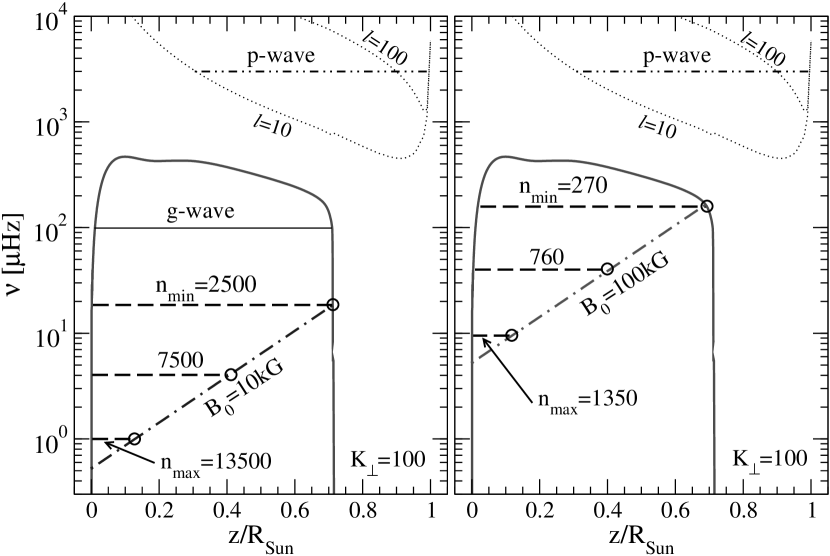
Figure 7: Relevant frequencies plotted against radial position within the sun. The solid curve gives the Brunt-Väisälä frequency, $N(z)$, while the dot-dashed lines are the Alfvén frequencies. Notice that $N(z)$ goes to zero at the solar center and the top of the radiative zone. The horizontal dashed lines represent the frequencies of magneto-gravity waves for several choices for the mode number, $n$, for fixed values $k_{x}=k_{\perp}=100/H$. As discussed in the text, resonances occur where the mode frequencies intersect the Alfvén frequency, indicated by circles in the figure. The two panels correspond to two choices for the magnetic field: 10 kG (left) and 100 kG (right). Minimum and maximum mode numbers are indicated, with $n_{\rm min}$ defined by the condition that its resonance occurs at the top of the radiative zone, $z_{r}(n_{\rm min})=0.7R_{\odot}$, and $n_{\rm max}$ having resonance at $z_{r}(n_{\rm max})=0.12R_{\odot}$. The dotted lines denote acoustic (Lamb) frequencies for $l=10$ and $100$ (see [10]) while the double-dot-dashed horizontal line represents the trapping region for a p-wave of frequency 3000 $\mu$Hz and $l=10$. The horizontal solid line represents the trapping region for a g-wave of frequency 100 $\mu$Hz.

It is instructive to examine the qualitative properties of the eigenvalue problem we have obtained. In the limit $B_{0}\to 0$ (and so $v_{A}\to 0$), Eq. (5) reduces to the standard evolution equation for ‘pure’ helioseismic $g$-modes, which is usually expressed in terms of the variable $v_{z}$ (which is related to $b_{z}$ through the relation $v_{z}=\omega b_{z}/k_{x}$). Since more detailed analyses – see Fig. 7 – show that $N$ rises from zero at the solar center, remains approximately constant $N\approx N_{0}$, through the radiative zone, and then falls to zero again at the bottom of the convective zone, these $g$-modes can be thought of as the eigen-modes of oscillations inside the cavity in between the two regions where $N$ goes through zero. For a given wave frequency, $\omega<N_{0}$, the turning points of this cavity are given by the condition $\omega\approx N$. For smaller $\omega$ the lower turning point gets closer to the solar center, $z\to 0$, and the upper one gets slightly closer to the bottom of the convective zone (CZ).

Conversely, if gravity is turned off ($N\to 0$), then Eq. (5) describes Alfvén waves, which oscillate with frequency $\omega=k_{x}v_{A}$ and propagate along the magnetic field lines. Notice that since $v_{A}\propto\rho^{-1/2}$ this frequency grows with $z$, since the density of the medium falls.

Keeping both magnetic and gravitational fields introduces qualitatively new behavior, as may be seen mathematically because equation (5) acquires a new singular point which occurs when the coefficient of the second-derivative term vanishes. Since this singularity appears at the Alfvén frequency,

$$\omega=k_{x}v_{A}$$ (8)

it can be interpreted as being due to a resonance between the $g$-modes and Alfvén waves. This resonance turns out to occur at a particular radius because the Alfvén frequency varies with radius while the $g$-mode frequency is independent of radius (see Fig. 7). The resonance occurs where the growing Alfvén mode frequency crosses the frequency of one of the $g$-modes, and the resulting waveforms would be expected to vary strongly at these points. The resonance can occur inside the radiative zone if the Alfvén frequency climbs high enough to cross a $g$-mode frequency before reaching the top of the radiative zone. Since $v_{A}\propto B_{0}$, whether this occurs or not depends on the field value, $B_{0}$.

The qualitative behaviour of the solutions can be seen from equation (5), and are oscillatory (or exponentially growing or damped) if the coefficient of the last term of this equation is positive (or negative). In the absence of magnetic fields, this leads to the onset of damping when $\omega>N(z)$. Since $N(z)$ vanishes at the top of the radiative zone, all modes necessarily become unstable there, and the corresponding instability gives rise to the convection which defines the convective zone. This is the usual picture of helioseismic $g$ modes. The presence of magnetic fields makes the coefficient of $b_{z}$ in eq. (5) go negative (for some modes) at smaller values of $z$, indicating the onset of an instability inside of the radiative zone.

The magnetic field leads to several new effects. First, the shortening of the cavity due to the presence of magnetic field causes the eigen-frequencies to depend on the magnetic field value. Second, there can be energy transfer between $g$-modes and Alfvén waves, within the narrow singular resonance layer, leading to the corresponding eigen-frequencies acquiring imaginary parts. Third, the nearer the upper boundary of MHD cavity is to the solar center, the stronger the $g$-modes are confined to the solar core.

More details of these waveforms can be obtained from a WKB-type analysis of the master Eq. (5). Near the solar center where $N^{2}\to 0$, if $(k_{x}v_{A})^{2}/\omega^{2}\ll 1$ one obtains the exponential solution $b_{z}\to e^{\pm k_{\perp}z}$. (Which combination of these solutions appears is fixed by boundary conditions, e.g. if $b_{z}(0)=0$ at the solar center we have $b_{z}\propto\sinh(k_{\perp}z)$.) One finds similar behaviour for the solution above the singular resonant layer, $z>z_{r}$, up to the top of the radiative zone. This exponential growth happens because of the exponential decrease of density (and so exponential increase in $v_{A}$) with $z$. The requirement for complex frequencies arises from the demand that the solution remain regular in the narrow Alfvén resonance layer.

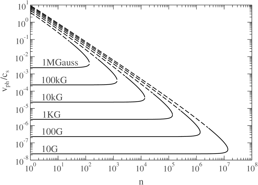
Figure 8: Plot of the $v_{ph}/c_{s}=\omega_{1}/k_{x}c_{s}$ against mode number, $n$, where $c_{s}$ is the adiabatic sound speed and $\omega_{1}$ is the real part of the eigenfrequencies, $\omega=\omega_{1}(1+id)$. Different curves correspond to different background magnetic field strengths, ${B}_{0}$. Solid lines represent resonances which are inside the radiative zone, whilst dashed lines correspond to unphysical modes whose resonances lie outside of the radiative zone.

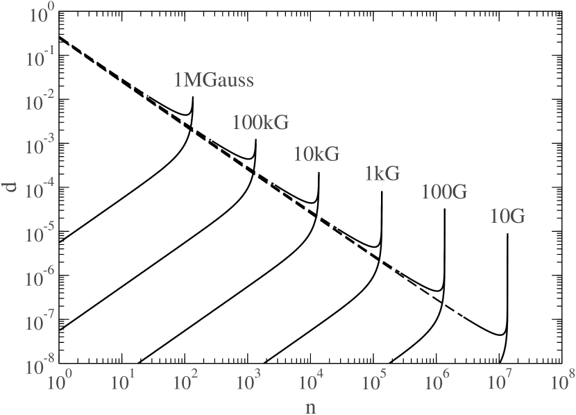
Figure 9: Plot of the $d$ against mode number, $n$, where $d$ gives the imaginary part of the eigenfrequencies, $\omega=\omega_{1}(1+id)$. Different curves correspond to different background magnetic field strengths, ${B}_{0}$. Solid lines represent resonances which are inside the radiative zone, whilst dashed lines correspond to unphysical modes whose resonances lie outside of the radiative zone.

Figures 8 and 9 present our numerical solution of the eigenvalue spectrum. Figure 8 plots $v_{ph}(n)/c_{s}=\omega_{1}/(c_{s}k_{x})$ vs mode number $n$ for various magnetic fields, $B_{0}$. Here $\omega_{1}$ is the real part of the eigenfrequency $\omega$, which in general is complex. (More about this later.) Figure 9 similarly plots the imaginary part of omega, Im $\omega=\omega_{1}\,d$ against mode number for the same magnetic fields. In both plots the parameter $\alpha=k_{x}/k_{\perp}$ is taken to be unity, where as before $k_{x}$ and $k_{\perp}^{2}=k_{x}^{2}+k_{y}^{2}$ are the mode’s wave-numbers in the transverse directions. In both figures a dashed line is used if the resonance of interest occurs above the top of the radiative zone (and so outside the domain of many of our approximations).

Both of the figures 8 and 9 show two branches of solutions up to a maximum mode number, as expected. Their dependence on $n$ can also be understood analytically from following approximate expressions [19]

$$\frac{\omega_{1}}{N}=\frac{2k_{\perp}H}{\pi n}\ln\left(\frac{4NH}{\alpha v_{Ac}}\frac{1}{\pi n}\right),$$

$$d=\frac{\ln\left|\tan(\pi/\gamma)\right|}{2\pi n}~{}.$$ (9)

These modes correspond to the branches of the figures 8 and 9 for which both $v_{ph}/c_{s}$ and $d$ fall with $n$. Analytic expressions are also possible for the other branch [19], and the spectrum in this case is

$$\omega_{1}=\frac{\alpha K_{\bot}v_{Ac}}{H},$$

$$d=-\left(\frac{\alpha v_{Ac}}{4NH}\right)^{2}\pi n\ln\left|\tan\frac{\pi}{\gamma}\right|~{}.$$ (10)

Note that for this branch $v_{ph}(n)/c_{s}$ is independent of the mode number, $n$, and $d$ grows with $n$, as is also seen in the figure.

In addition to requiring the resonance to occur in the radiative zone (the solid line in the figures), the validity of our approximations also demand the frequency not to be smaller than $10^{-5}$ s^-1 due to our neglect of the 27-day period solar rotation. Inspection of Fig. 8 shows that these two conditions are consistent with one another for a reasonably large range of modes only for magnetic fields larger than a kG or so.

The resonance alluded to above appears causes two distinctive features to appear in these solutions. First, the eigenfrequencies are complex, implying both damped and exponentially-growing modes. Second, the eigenmodes are not smooth as functions of $z$ about the singular resonant point, $z=z_{r}(n,k_{x},k_{y})$, whose position depends on the quantum numbers of the mode in question.

The necessity for complex frequencies imply the mode functions grow exponentially in amplitude with time. This signals an instability in the physics which pumps energy into these resonances, and this section aims to discuss the nature of this instability, and the physical interpretation to be assigned to the imaginary part, $d$. Exponentially-growing instabilities within an approximate (e.g. linearized) analysis reflect the system’s propensity to leave the small-field regime, on which the validity of the approximate analysis relies. The question becomes: where does the instability lead, and what previously-neglected effects stabilize the runaway behaviour?

In the present instance the normal modes are strongly peaked near the resonant radii, and the energy flow near these radii is directed along the resonance plane, much as would be true for a pure Alfvén wave. Since helioseismic waves are likely generated by the turbulence at the bottom of the convective zone, it is natural to imagine starting the system with a regular helioseismic $g$-mode and asking how it evolves. In this case the resonance allows the energy in this mode to be funnelled into the Alfvén wave, and so to be channelled along the magnetic field lines away from the solar equatorial plane. The imaginary part of the frequency, $\Gamma=\hbox{Im}\,\omega=\omega_{1}\,d$, describes the rate at which the Alfvén mode is excited in this process.

Once excited, the mode amplitudes near the resonances grow until the energy in them becomes dissipated by effects which are not captured by the approximate discussion we present here. The rate for this dissipation must grow as the mode amplitude grows, until it equals the production rate, $\Gamma$, at which point a steady state develops and the mode growth is stabilized. Because the resonant mode grows until its damping rate equals its production rate, it suffices to know the mode’s growth rate in order to determine the overall on-resonance amplitude. If the mode stabilizes once it is large enough to require a nonlinear analysis, then the final production and dissipation rates may be very different from the linearized expressions derived above. If, on the other hand, the modes saturate at comparatively small amplitudes by dissipating energy into non-hydrodynamical modes (such as by Landau damping), then it can happen that the stabilized mode amplitude is not large enough to significantly change the linearized prediction for its production rate.

Figure 10: A plot of the resonant position, $z_{r}(n)$, vs mode number $n$ for different magnetic fields in the range $B_{0}=$ 10G–1MG.

Fig. 10 plots the position, $z_{r}(n)$, predicted for the case of longitudinal wave propagation ($k_{y}=0$) and for magnetic fields in the range $B_{0}=$10G–1MG. (The same result for an obliquely-propagating wave with $k_{y}\neq 0$ is produced by a larger value for $B_{0}$.) This plot is the analog of Figs. 5a,b in [33]. Knowing the position of the resonances also permits us to determine the distance between them. This quantity is relevant to the propagation of particles like neutrinos through the resonant waves. The spacing is:

$$z_{r}(n+1)-z_{r}(n)=\left(\frac{k_{x}}{k_{\perp}}\right)\frac{\pi H\,v_{Ac}\gamma}{c_{s}\sqrt{\gamma-1}}\;e^{z_{r}(n)/2H}~{}.$$ (11)

This dependence of this quantity on mode number, $n$, is shown in Fig. 11 for longitudinal wave propagation, $k_{y}=0$, and for different magnetic field values. From this figure we see, in the region $z_{r}\mbox{\raisebox{-2.58334pt}{~{}$\stackrel{{\scriptstyle>}}{{\sim}}$~{}}}0.3R_{\odot}$, that the distance between layer positions grows with magnetic field and with distance from the solar center. Both of these features were already seen in preliminary WKB calculations of the resonances (see Figs. 7a, 7b of ref. [33]), and our present numerics also confirm that the spacing is approximately proportional to $B_{0}$ for $z\mbox{\raisebox{-2.58334pt}{~{}$\stackrel{{\scriptstyle>}}{{\sim}}$~{}}}0.3R_{\odot}$, that was seen earlier.

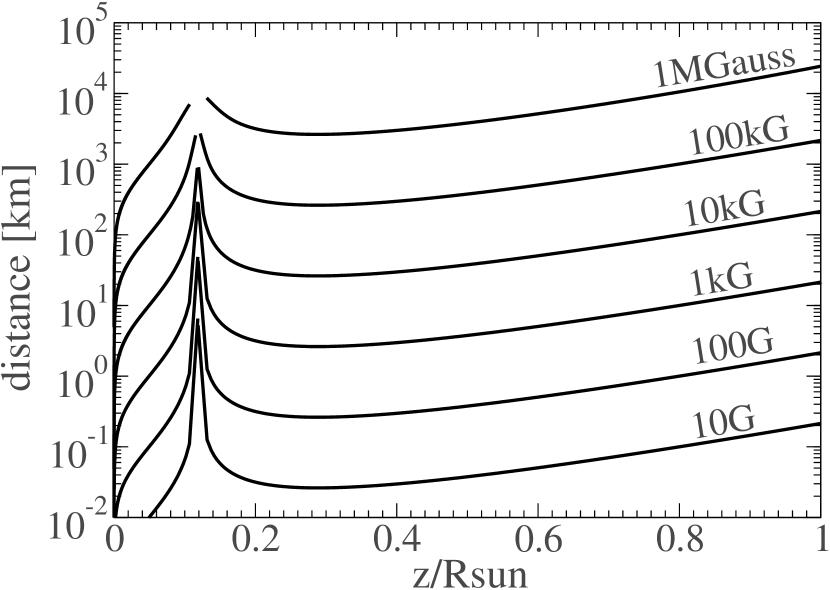
Figure 11: The distance between neighbouring Alfvén resonant layers vs the position of the layer within the solar interior.

An approximate expression for the differenece between adjacent resonance positions is given by

$$z_{r}(n+1)-z_{r}(n)\approx\frac{2H}{\mid n\mid}~{},$$ (12)

where the inverse mode number $\mid n\mid^{-1}$ is proportional to the background magnetic field $\sim B_{0}$.

Numerically, it is noteworthy that the spacing between resonances can be hundreds of kilometers. This is significant because this is close to the resonant oscillation length, $l_{osc}^{res}$, for $E\sim\rm{MeV}$ neutrinos, if – as now seems quite likely – resonant LMA oscillations are responsible for explaining the solar neutrino problem since

$$l_{osc}^{res}=\frac{250~{}\rm{km}~{}(E/\rm{MeV})}{\Delta m^{2}_{5}\sin 2\theta}\,,$$ (13)

where $\Delta m^{2}_{5}=\Delta m^{2}/10^{-5}~{}\hbox{eV}^{2}$. Repeatedly perturbing neutrinos over distance scales comparable to $l_{osc}^{res}$ has long been known to be a prerequisite for disturbing the standard MSW picture of oscillations in the solar medium. This raises the possibility – recently explored in more detail in ref. [15] – that $g$-mode/Alfvén resonances can alter neutrino propagation. If so, the observation of resonant oscillations of solar neutrinos may provide some direct information about the properties of the MG waves we discuss here.

4 Summary

Within the approximations given it appears that sufficiently large magnetic fields can cause significant changes to the profiles of helioseismic $g$-waves, while not appreciably perturbing helioseismic $p$-waves. The comparatively large $g$-wave effects arise because of a resonance which occurs between the $g$-modes and magnetic Alfvén waves in the solar radiative zone. Although the radiative-zone magnetic fields required to produce observable effects are larger than are often considered – more than a few kG – they are not directly ruled out by any observations.

Although the density profiles at their maxima could have amplitudes as large as a few percent or more on resonance, we do not believe the corresponding radiative-zone magnetic fields can yet be ruled out by comparison with helioseismic data, since the density excursions are sufficiently narrow (hundreds of kilometers) as to evade the assumptions which underlie standard helioseismic analyses.

For magnetic fields in the 10 kG range, the best hopes for detection of the resonant waves may be through their influence on neutrino propagation. This influence essentially arises because the presence of strong density variations affects the solar neutrino survival probability, with a corresponding change in the resulting solar neutrino fluxes. As described above, and shown in ref. [15], the measurement of neutrino properties at KamLAND provides new information about fluctuations in the solar environment on correlation length scales close to 100 km, to which standard helioseismic constraints are largely insensitive. We have already seen how the determination of neutrino oscillation parameters from a combined fit of KamLAND and solar data depends strongly on the magnitude of solar density fluctuations.

Since the resonances rely on the condition that ${\vec{B}}\perp\nabla\rho$, there are several magnetic-field geometries to which our analysis might apply, and it is instructive to consider two illustrative examples to see what kinds of observable effects might be possible. Suppose first that, in spherical coordinates $(r,\theta,\phi)$, we imagine $B_{r}\approx 0$ but $B_{\theta}\neq 0$. Then the field is always perpendicular to a radial density gradient and the resonance we find might be expected to arise in all directions as one comes away from the solar center. In this case the solar $g$-modes would tend to be trapped behind the resonance, and so are kept away from the solar surface even more strongly than is normally expected. This would make the prospects for their eventual detection very poor.

Alternatively, if the magnetic field has more of a dipole form it might be imagined that the condition ${\vec{B}}\perp\nabla\rho$ only holds near the solar equatorial plane, and not near the solar poles. In this case a more detailed calculation is needed in order to determine the resulting wave form. This kind of geometry could have interesting consequences for the solar neutrino signal, because in this case the deviation from standard MSW analyses only arises for neutrinos which travel sufficiently close to the solar equatorial plane. Given the roughly 7-degree inclination of the Earth’s orbit relative to the plane of the solar equator, there is a possibility of observing a seasonal dependence in the observed solar neutrino flux. Since the presence of the MG resonance tends to decrease the MSW effect, the prediction would be that the observed rate of solar electron-neutrino events is maximized when the Earth is closest to the solar equatorial plane (December and June) and is minimized when furthest from this plane (March and September).

References

- [1] Solar data were reviewed in the talks by M. Smy, A. Hallin, T. Kirsten, V.Gavrin, K.Lande at the XXth International Conference on Neutrino Physics and Astrophysics, http://neutrino2002.ph.tum.de/
- [2] Q. R. Ahmad et al. [SNO Collaboration], Phys. Rev. Lett. 89, 011301 (2002); Phys. Rev. Lett. 89, 011302 (2002).
- [3] S. Fukuda et al. [SuperKamiokande Collaboration], Phys. Lett. B 539, 179 (2002)
- [4] Atmospheric data were reviewed in the talks by M. Shiozawa and M. Goodman at the XXth International Conference on Neutrino Physics and Astrophysics, http://neutrino2002.ph.tum.de/
- [5] Y. Fukuda et al. [Super-Kamiokande Collaboration], Phys. Rev. Lett. 81, 1562 (1998)
- [6] http://www.awa.tohoku.ac.jp/html/KamLAND/
- [7] http://neutrino.kek.jp/
- [8] J. Bahcall, “Neutrino Astrophysics” Cambridge University Press, 1989.
- [9] V. Castellani et al, Nucl. Phys. Proc. Suppl. 70 (1999) 301
- [10] J. Christensen-Dalsgaard, Lecture Notes available at http://bigcat.obs.aau.dk/ jcd/oscilnotes/. See also “Helioseismology,” arXiv:astro-ph/0207403
- [11] A. B. Balantekin, J. M. Fetter and F. N. Loreti, Phys. Rev. D 54, 3941 (1996)
- [12] H. Nunokawa, A. Rossi, V. B. Semikoz and J. W. Valle, Nucl. Phys. B 472 (1996) 495
- [13] C.P. Burgess and D. Michaud, Ann. Phys. (NY) 256 (1997) 1
- [14] P. Bamert, C. P. Burgess and D. Michaud, Nucl. Phys. B 513, 319 (1998)
- [15] Burgess C. P., Dzhalilov N. S., Maltoni M., Rashba T. I., Semikoz V. B., Tortola M., Valle J. W. F., 2003, Ap. J. , 588, L65 (hep-ph/0209094).
- [16] A.B. Balantekin and H. Yuksel, Phys. Rev. D68 (2003) 013006; M.M. Guzzo, P.C. de Holanda and N. Reggiani, Phys. Lett. B569 (2003) 45.
- [17] C.P. Burgess, N.S. Dzhalilov, M. Maltoni, T.I. Rashba, V.B. Semikoz, M. Tórtola and J.W.F. Valle, (arXiv:hep-ph/0310366).
- [18] S.N. Ahmed et.al. (The SNO Collaboration) arXiv:nucl-ex/0309004.
- [19] C.P. Burgess, N.S. Dzhalilov, T.I. Rashba, V.B. Semikoz and J.W.F. Valle, M.N.R.A.S. (to appear) (astro-ph/0304462).
- [20] L. Wolfenstein, Phys. Rev. D 17, 2369 (1978); S. P. Mikheev and A. Y. Smirnov, Sov. J. Nucl. Phys. 42 (1985) 913
- [21] M. Maltoni, T. Schwetz, M. A. Tortola and J. W. Valle, arXiv:hep-ph/0207227. Other recent analyses of solar data can be found in ref. [22] and referencs therein.
- [22] G. L. Fogli et al, arXiv:hep-ph/0206162; J. N. Bahcall, M. C. Gonzalez-Garcia and C. Pena-Garay, arXiv:hep-ph/0204314; A. Bandyopadhyay, S. Choubey, S. Goswami and D. P. Roy, Phys. Lett. B 540, 14 (2002); Mod. Phys. Lett. A 17, 1455 (2002); V. Barger et al, Phys. Lett. B 537, 179 (2002); P. C. de Holanda and A. Y. Smirnov, arXiv:hep-ph/0205241; P. Creminelli, G. Signorelli and A. Strumia, JHEP 0105, 052 (2001)
- [23] S. Couvidat, S. Turck-Chieze and A. G. Kosovichev, arXiv:astro-ph/0203107.
- [24] A. Friedland and A. Gruzinov, preprint (astro-ph/0211377).
- [25] Cowling T.G., 1945, MNRAS, 105, 166
- [26] Bahcall J. N., Ulrich R., 1971, ApJ, 170, 593
- [27] Parker E. N., 1979, Cosmical magnetic fields (Oxford: Clarendon Press)
- [28] Boruta N., 1996, Ap. J. , 458, 832
- [29] Kitchatinov L. L., Jardin M., Collier Cameron A., 2001, A&A, 374, 250
- [30] Mestel L., Weiss N. O., 1987, MNRAS, 226, 123
- [31] Ionson J., 1978, Ap. J. , 226, 650; Ap. J. , 254, 318; Ap. J. , 276 357.
- [32] Hollweg J. V., 1987a, Ap. J. , 312, 880; Ap. J. , 320, 875.
- [33] Dzhalilov N. S., Semikoz V. B., 1998, unpublished (astro-ph/9812149)