Constraints on Large Extra Dimensions with
Bulk Neutrinos

Abstract

We consider right-handed neutrinos propagating in $\delta$ (large) extra dimensions, whose only coupling to Standard Model fields is the Yukawa coupling to the left-handed neutrino and the Higgs boson. These theories are attractive as they can explain the smallness of the neutrino mass, as has already been shown. We show that if $\delta$ is bigger than two, there are strong constraints on the radius of the extra dimensions, resulting from the experimental limit on the probability of an active state to mix into the large number of sterile Kaluza-Klein states of the bulk neutrino. We also calculate the bounds on the radius resulting from requiring that perturbative unitarity be valid in the theory, in an imagined Higgs-Higgs scattering channel.

I Introduction

The Standard Model (SM) of high energy physics suffers from the gauge hierarchy problem, which is the fine tuning required to maintain a low electroweak scale ($M_{EW}\sim 10^{3}$ GeV) in the presence of another seemingly fundamental scale, the Planck scale (the scale of gravity, $M_{pl}\sim 10^{19}$ GeV). Supersymmetry, technicolor and more recently extra (space) dimensions have been proposed to address the hierarchy problem.

Recent neutrino oscillation experiments have suggested a non-zero neutrino mass, with the best fit values of the mass differences and mixing angles given by Fukuda:1998mi ; Ahmad:2002ka ; Wolfenstein:1977ue ; Bahcall:2002hv

$$\Delta m^{2}_{\rm Solar} = 7\times 10^{-5}~{}{\rm eV^{2}}\ ,\ \ \ \tan^{2}\theta_{Solar}=0.4\ ,$$

$$\Delta m^{2}_{\rm Atm} = 2.5\times 10^{-3}~{}{\rm eV^{2}}\ ,\ \ \ \tan^{2}\theta_{Atm}=1\ .$$ (1)

The oscillation between the three active flavors, $\nu_{e}$,$\nu_{\mu}$,$\nu_{\tau}$, in the SM, accommodates this satisfactorily, with $\Delta m^{2}_{\rm Solar}=|m_{1}^{2}-m_{2}^{2}|$ and $\Delta m^{2}_{\rm Atm}=|m_{2}^{2}-m_{3}^{2}|$, the $m_{i}$ being the physical masses. If the $m_{i}$ are also assumed to be of the same order of magnitude as the mass differences, it is quite challenging to explain why it is that the neutrinos are so light compared to the other leptons.

It has been shown Arkani-Hamed:1998rs ; Antoniadis:1998ig that if there are other Large Extra Dimensions (LED) in addition to our usual four space-time dimensions, we could potentially solve the gauge hierarchy problem. It was then pointed out Dienes:1998sb ; Arkani-Hamed:1998vp ; Dvali:1999cn that the smallness of the neutrino mass is naturally explained if right-handed neutrinos that propagate in some $\delta$ number of these extra dimensions are introduced. We will refer to such neutrinos, which are SM gauge singlets, as “bulk neutrinos”, as is the usual practice. Various aspects of theories with bulk neutrinos have been analyzed in Ref. Mohapatra:1999zd .

If bulk right-handed neutrinos are responsible for the smallness of the neutrino mass, we ask in this paper, what the constraints on such a model might be. We will find that the experimental constraints on the probability of an active neutrino to oscillate into sterile bulk neutrinos, can give us a lower bound on the inverse radius ($1/R$) of such extra dimensions, especially if $\delta>2$. We will also require that perturbative unitarity in two-to-two scattering of Higgs bosons be preserved in the theory. We will include the tower of Kaluza-Klein states as intermediate states, and again find that for $\delta>2$ it results in a strong bound on $1/R$.

We will take the view, as in Ref. Davoudiasl:2002fq , that the standard three-active-flavor oscillation explains the data in Eq. (1), and that the mixing to sterile bulk neutrinos are small enough to evade experimental constraints. Here we extend the analysis to $\delta>1$ and show that strong bounds on $1/R$ can result in that case. However, a precise calculation of the bound will not be possible when $\delta>2$ due to sensitivity on the cutoff scale, implying a dependence on how one completes the extra dimensional (effective) theory that we will work with. As pointed out in Ref. Davoudiasl:2002fq an alternative approach Dienes:1998sb ; Dvali:1999cn , wherein Eq. (1) is explained by the oscillation of the active species predominantly into sterile bulk neutrinos, appears to be disfavored by the Sudbury Neutrino Observatory (SNO) Ahmad:2002ka neutral current data.

In order to constrain theories with neutrinos in the bulk, other processes have also been considered in the literature Ioannisian:1999cw including muon lifetime, pion decay, flavor violation, beta decay in nuclei, muon $g-2$, supernova energy loss and big bang nucleosynthesis. Some phenomenological implications are also considered in Ref. DeGouvea:2001mz .

The rest of the paper is organized as follows. We will introduce the extra dimensional theory with bulk neutrinos in Sec. II, write down the equivalent four dimensional Kaluza-Klein theory with particular focus on the interaction of the right-handed bulk neutrino with the Higgs field and the left-handed neutrino, and diagonalize the neutrino mass matrix. In Sec. III, we will find the bounds on the radius of the extra dimensions from limits on neutrino oscillation into sterile states, and in Sec. IV, from unitarity considerations in Higgs-Higgs scattering. Our conclusions are given in Sec. V. We will present an alternate approach to the diagonalization of the neutrino mass matrix in Appendix A, and give in Appendix B some detailed formulas that we use in deriving the unitarity bound.

II Right-handed Neutrinos in Extra Dimensions

To address the gauge hierarchy problem, Arkani-Hamed, Dimopoulos and Dvali (ADD) Arkani-Hamed:1998rs postulate that the Standard Model (SM) fields are confined to a 4 dimensional (4-D) sub-space (brane) in an extra dimensional world of $4+n$ total dimensions. ADD take the view that the only fundamental scale in nature is $M_{*}$, which is of the order of $M_{EW}$, and the apparent 4-D gravity scale ($M_{pl}$) is then given by

$$M_{pl}^{2}=M_{*}^{2+n}V_{n},$$ (2)

where, $V_{n}$ is the volume of the (compact) extra dimensional space. In the simple case of each of the compact extra dimensions being of equal radius $R^{\prime}$, we have $V_{n}\sim{R^{\prime}}^{n}$. Thus ADD argue that $M_{pl}$ appears to be a large scale from a 4 dimensional perspective simply because the volume $V_{n}$ is large. In other words, the explanation of why $M_{pl}$ is large is recast to stabilizing $R^{\prime}$ at a large value, so that $V_{n}$ is large.

It should be pointed out that for a given $M_{*}$, if the $n$ compact dimensions have equal radii $R^{\prime}$, Eq. (2) implies a particular value of $R^{\prime}$. However, if it happens that there are two sets of compact extra dimensions of unequal size, $\delta$ of them ($\delta\leq n$) with radius $R$, and the other $(n-\delta)$ with radius $R^{\prime}$, then we have in this case, $V_{n}\sim{R^{\prime}}^{(n-\delta)}\,R^{\delta}$. We can in this case think of $R$ as an independent variable with $R^{\prime}$ being determined by Eq. (2).

We consider the ADD framework, to which is added three (one for each generation) bulk fermions, $\Psi^{\alpha}(x^{\mu},\underline{y})$, that propagate in 4+$\delta$ dimensions ($\delta$ of them compact with radius $R$), where the indices $\alpha$, $\beta=(1,~{}2,~{}3)$ denote the three generations, and $\underline{y}$ stands for $\{y^{1},...,y^{\delta}\}$. Since the higher dimensional Lorentz invariance is reduced to our 4-dimensional invariance by the presence of the brane (where SM fields are localized), we are interested only in keeping track of the 4-dimensional Lorentz transformation property of $\Psi$ along the direction of the brane. We consider the situation where the SM fields couple only to 2 components of $\Psi$, denoted as $\psi_{R}(x^{\mu},\underline{y})$, and transforming as a right-handed 2-component Weyl spinor under 4-D Lorentz transformations. For example, for $\delta=1$, we denote a 5 dimensional (4 component) spinor as

$$\Psi^{\alpha}(x^{\mu},y)=\pmatrix{\psi_{L}^{\alpha}(x^{\mu},y)\cr\psi_{R}^{\alpha}(x^{\mu},y)},$$ (3)

where the $L$ and $R$ subscripts make explicit the four dimensional Lorentz property, and in particular, $\psi^{\alpha}_{L,R}$ each transforms as a (2 component) Weyl spinor. In the following, we will keep the formalism general enough to include arbitrary number of extra dimensions.

We can split the Lagrangian into a bulk piece and a brane piece,

$${\cal S} = \int d^{4}x~{}d^{\delta}y~{}\left[{\cal L}_{\rm Bulk}~{}+~{}\delta(\underline{y})\,{\cal L}_{Brane}\right].$$ (4)

${\cal L}_{\rm Bulk}$ contains the Einstein-Hilbert bulk gravity term (which we will not show explicitly, but can be found, for example, in Ref. Giudice:1998ck ), the kinetic energy term for the bulk neutrino field $\Psi(x^{\mu},\underline{y})$ and in general, a bulk Majorana mass term for $\Psi$, which for simplicity we will omit (see Ref. Dienes:1998sb for implications of a nonzero bulk Majorana mass). ${\cal L}_{\rm Brane}$ contains the SM Lagrangian plus an interaction term between SM fields and $\psi_{R}$,

$${\cal L}_{\rm Bulk} \supset \bar{\Psi}^{\alpha}\,i\Gamma^{M}D_{M}\Psi^{\alpha},$$

$${\cal L}_{\rm Brane} \supset {\cal L}_{\rm SM}-\left(\frac{\Lambda^{\nu}_{\alpha\beta}}{\sqrt{M_{*}^{\delta}}}~{}h\,\psi_{R}^{\beta}\,\nu_{L}^{\alpha}+h.c.\right),$$ (5)

$${\cal L}_{\rm SM} \supset \bar{\nu}_{L}^{\alpha}\,i\gamma^{\mu}D_{\mu}\nu_{L}^{\alpha}+\left(\frac{g}{\sqrt{2}}\,\bar{\nu}_{L}^{\alpha}\,\gamma^{\mu}e_{L}^{\alpha}W_{\mu}^{+}+h.c\right)+...\,,$$

where, $\Lambda^{\nu}_{\alpha\beta}$ is an $O(1)$ Yukawa coupling constant. It should be kept in mind that $\psi_{R}$ is a function of ($x^{\mu},\underline{y}$) whereas the SM fields are functions of $x^{\mu}$ only. The index $M$ runs over {$x^{\mu},\underline{y}$}.

We can perform a Kaluza-Klein (KK) expansion of the 4+$\delta$ dimensional theory and obtain an equivalent 4-D theory by writing,

$$\psi^{\alpha}_{R}(x^{\mu},\underline{y})=\sum_{\underline{n}}~{}{\psi_{R}^{\alpha}}^{(\underline{n})}(x^{\mu})~{}f_{\underline{n}}(\underline{y}),$$ (6)

where, $\underline{n}=(n_{1},...,n_{\delta})$ is a vector in “number space”, $\psi^{(\underline{n})}$ are the KK modes and $f_{\underline{n}}(\underline{y})$ is a complete set over $\underline{y}$. A similar expansion is made for $\psi^{\alpha}_{L}$. To reduce clutter, we will simply write $n$ and $y$ for $\underline{n}$ and $\underline{y}$ respectively. We will use the notation $n=(0,1,...)$ and $\hat{n}=(1,...)$ ($\hat{n}$ excludes 0). $f_{n}$ is an orthonormal set,

$$\int_{0}^{2\pi R}d^{\delta}y~{}~{}f_{n}^{*}(y)f_{m}(y)=\delta^{nm},$$ (7)

and a convenient choice is,

$$f_{n}(y)=\frac{e^{i\frac{n.y}{R}}}{\sqrt{\frac{S_{\delta-1}}{\delta}R^{\delta}}}=\frac{e^{i\frac{n.y}{R}}}{\sqrt{V_{\delta}}},$$ (8)

with $S_{\delta-1}$ the surface “area” of a unit sphere in $\delta$ dimensions, and $V_{\delta}\equiv\frac{S_{\delta-1}}{\delta}R^{\delta}$ is the volume of the extra dimensional space.

We define the fields Davoudiasl:2002fq ,

$$\nu^{\alpha}_{R} \equiv \psi_{R}^{\alpha(0)},$$

$$\nu_{R}^{\alpha(\hat{n})} \equiv \frac{1}{\sqrt{2}}\left(\psi_{R}^{\alpha(\hat{n})}+\psi_{R}^{\alpha(-\hat{n})}\right),$$

$$\nu_{L}^{\alpha(\hat{n})} \equiv \frac{1}{\sqrt{2}}\left(\psi_{L}^{\alpha(\hat{n})}+\psi_{L}^{\alpha(-\hat{n})}\right)\ .$$

We substitute the KK expansion for the bulk fields $\psi_{R}^{\alpha}$ and $\psi_{L}^{\alpha}$ into Eq. (5) to get the equivalent 4-D theory,

$${\cal L}^{(4)}={\cal L}_{SM}-\sum_{\alpha=1}^{3}\sum_{\hat{n}}\left[\frac{|\hat{n}|}{R}\left(\nu_{R}^{\alpha(\hat{n})}\nu_{L}^{\alpha{(\hat{n})}}+h.c.\right)\right]-\sum_{\alpha,\beta=1}^{3}\left[\frac{m_{\nu}^{\alpha\beta}}{v}\left(h\nu_{R}^{\alpha}\nu_{L}^{\beta}+\sum_{\hat{n}}\sqrt{2}h\nu_{R}^{\alpha(\hat{n})}\nu_{L}^{\beta}\right)+h.c.\right],$$ (9)

where, $|\hat{n}|~{}\equiv~{}\sqrt{n_{1}^{2}+...+n_{\delta}^{2}}$. We note here that in ${\cal L}^{(4)}$, there is a tower of KK states $(\nu_{L}^{(\hat{n})},\nu_{R}^{(\hat{n})})$ with Dirac masses approximately equal to $|\hat{n}|/R$. Henceforth, we will assume that unless noted otherwise, repeated generation indices $\alpha,\beta,i,j$, and KK indices $n,\hat{n},m$, are summed over.

With $SU(2)$ broken by the Higgs mechanism, by the Higgs field acquiring a vacuum expectation value (VEV), $\left<h\right>=v$, we have the neutrino masses given by,

$$m_{\nu}^{\alpha\beta}\equiv\frac{\Lambda^{\nu}_{\alpha\beta}~{}v}{\sqrt{\frac{S_{\delta-1}}{\delta}(M_{*}R)^{\delta}}}=\frac{\Lambda^{\nu}_{\alpha\beta}~{}v}{\sqrt{V_{\delta}M_{*}^{\delta}}},$$ (10)

and $m_{\nu}$ can be much smaller than $M_{EW}\sim v$, if $V_{\delta}$ is large. We show in Table 1 an estimate of the order of magnitude of the $\Lambda^{\nu}_{\alpha\beta}$ that one needs in order to get neutrino masses of $O(10^{-2})$ eV. The $1/R$ values are chosen anticipating the constraint from neutrino oscillation that we will derive in Sec. III. We note that $\delta=1$, though the case most studied, requires an unnaturally small $\Lambda$. We will therefore include $\delta>1$ in our analysis.

Table 1: Estimate of $\Lambda^{\nu}_{\alpha\beta}$. ($M_{*}$ = 1 TeV)

$\delta$	$\frac{1}{R}\ (eV)$	$\Lambda^{\nu}_{\alpha\beta}$
1	1	$10^{-6}$
2	1	0.1
3	$10^{3}$	1

II.1 Truncation of the KK sum

Though $\hat{n}_{i}$ can in principle go up to $\infty$, leading to an infinite tower of Dirac states with masses $|\hat{n}|/R$, we take the view that this extra dimensional field theory description is valid up to the cutoff scale $M_{*}$, and therefore truncate the $\hat{n}_{i}$ such that the highest KK mass is $M_{*}$. We define $N$ to be $N/R=M_{*}$. For $\delta>1$, the state with mass $\frac{|\hat{n}|}{R}$ can be degenerate, and we denote the degeneracy at the $\hat{n}^{\rm th}$ level by $d_{\hat{n}}$. (Strictly speaking, we should denote this as $d_{|\hat{n}|}$, but we will just write this as $d_{\hat{n}}$.) For example, for $\delta=3$, the state with mass $1/R$ has $d_{1}=3$, corresponding to $(\hat{n}_{1},\hat{n}_{2},\hat{n}_{3})\rightarrow(1,0,0),\ (0,1,0)\ {\rm and}\ (0,0,1)$, all of which have the same mass. For large $|\hat{n}|$, the leading power dependence of $d_{\hat{n}}$ in $\delta$ extra dimensions is given by $d_{\hat{n}}=c_{\hat{n}}|\hat{n}|^{\delta-1}$, where the $c_{\hat{n}}$ are $O(1)$ numbers. We define $d_{0}\equiv 1$.

For large $|\hat{n}|$, we can think of the $\hat{n}_{i}$ as a continuum and the leading behavior is given by the surface of the $(\delta-1)$-sphere of radius $|\hat{n}|$ in number space,

$$d_{\hat{n}}\sim S_{\delta-1}|\hat{n}|^{\delta-1}\ \ \ \ \ \ {\rm(in\ \delta\ dimensions).}$$ (11)

$$d^{\delta=1}_{\hat{n}}=1,\ \ \ \ \ \ d^{\delta=2}_{\hat{n}}\sim 2\pi\hat{n},\ \ \ \ \ \ d^{\delta=3}_{\hat{n}}\sim 4\pi\hat{n}^{2}\ .$$

For example, for $\delta=3$, $d_{\hat{n}}\sim 4\pi|\hat{n}|^{2}$, which is the surface of the 2-sphere with radius $|\hat{n}|$. Thus, $N$ is the radius of the biggest sphere in $\{n_{i}\}$ space such that $N/R=M_{*}$. We will often use the continuum approximation for estimating various quantities.

The sum over the KK states of certain quantities can be divergent and can depend on $N$. We will elaborate more on this later, and we will see that the probability of active neutrinos oscillating into heavier sterile KK states can depend on N, especially strongly for $\delta>3$.

II.2 Mass Matrix Diagonalization

At the outset, we can make the Yukawa coupling in Eq. (9) diagonal in generation space ($\alpha,\beta$) with the rotations Davoudiasl:2002fq ,

$$\nu_{L}^{\alpha}=l^{\alpha i}\nu_{L}^{\prime i} \ \ \ \nu_{R}^{\alpha}=(r^{\alpha i})^{*}\nu_{R}^{\prime i}\ ,$$ ,

$$\nu_{R}^{\alpha(\hat{n})}=(r^{\alpha i})^{*}\nu_{R}^{\prime i(\hat{n})} \ \ \ \nu_{L}^{\alpha(\hat{n})}=r^{\alpha i}\nu_{L}^{\prime i(\hat{n})}\ ,$$ ,

$$e_{L}^{\alpha}=l_{e}^{\alpha i}e_{L}^{\prime i} \ \ \ e_{R}^{\alpha}=(r_{e}^{\alpha i})^{*}e_{R}^{\prime i}\ ,$$ ,

where the unitary matrices $l$ and $r$ are chosen to diagonalize $m_{\nu}^{\alpha\beta}$, so that, $(r^{\alpha i})^{*}~{}m_{\nu}^{\alpha\beta}~{}(l^{\beta j})=m_{\nu}^{i}\delta^{ij}$. Similarly, $l_{e}$ and $r_{e}$ are chosen to diagonalize the electron-type mass matrix. After these rotations, Eq. (9) becomes,

$${\cal L}^{(4)}={\cal L}_{SM}-\frac{|\hat{n}|}{R}\left(\nu_{R}^{\prime i(\hat{n})}\nu_{L}^{\prime i(\hat{n})}+h.c.\right)-\left[\frac{m_{\nu}^{i}}{v}\left(h\nu_{R}^{\prime i}\nu_{L}^{\prime i}+\sum_{\hat{n}}\sqrt{2}h\nu_{R}^{\prime i(\hat{n})}\nu_{L}^{\prime i}\right)+h.c.\right]\ .$$ (12)

In the usual way, the charged current interactions now become proportional to the MNS matrix Maki:mu ,

$$V_{MNS}\equiv l_{e}^{\dagger}\,l\ .$$ (13)

By defining the Dirac spinors,

$$\nu^{\prime i}\equiv\pmatrix{\nu_{L}^{\prime i}\cr\nu_{R}^{\prime i}},~{}~{}\nu^{\prime i(1)}\equiv\pmatrix{\nu_{L}^{\prime i(1)}\cr\nu_{R}^{\prime i(1)}}~{}.~{}.~{}.~{}\nu^{\prime i(n)}\equiv\pmatrix{\nu_{L}^{\prime i(n)}\cr\nu_{R}^{\prime i(n)}},$$ (14)

we can rewrite Eq. (12) as,

$${\cal L}^{(4)}={\cal L}_{SM}-\frac{|\hat{n}|}{R}\bar{\nu^{\prime i(\hat{n})}}\nu^{\prime i(\hat{n})}-\frac{m_{\nu}^{i}}{v}\left[h\bar{\nu^{\prime i}}\nu^{\prime i}+\sqrt{2}h\left(\sum_{\hat{n}}\bar{\nu^{\prime i(\hat{n})}}P_{L}\nu^{\prime i}+h.c.\right)\right],$$ (15)

where $P_{L(R)}\equiv\left(1\mp\gamma_{5}\right)$.

To reduce clutter, in the rest of this section, we will suppress writing the generation index $i$ and the prime on the fields. Thus for each $i=1,2,3$, the mass matrix in KK space can be diagonalized independently using the procedure described next.

For each $i$, the neutrino mass term obtained by setting $\left<h\right>=v$ is,

$${\cal L}^{(4)}_{\rm mass}=\bar{\nu_{D}}~{}{\cal M}_{D}~{}\nu_{D},$$ (16)

with $(\nu_{D})^{T}=(\nu~{}\nu^{(1)}~{}...~{}\nu^{(\hat{n})}~{}...)$ and the mass matrix is given by,

$${\cal M}_{D}=\pmatrix{m_{\nu}&\sqrt{2}m_{\nu}P_{R}&.&.&.&\sqrt{2}m_{\nu}P_{R}&.&.&.\cr\sqrt{2}m_{\nu}P_{L}&\frac{1}{R}&&&&&&&\cr.&&.&&&&&&\cr.&&&.&&&&&\cr.&&&&.&&&&\cr\sqrt{2}m_{\nu}P_{L}&&&&&(\frac{|\hat{n}|}{R})_{d_{\hat{n}}\times d_{\hat{n}}}&&&\cr.&&&&&&.&&\cr.&&&&&&&.&\cr.&&&&&&&&\frac{|N|}{R}\cr}.$$ (17)

We keep in mind that the ${\hat{n}}^{\rm th}$ state is degenerate with degeneracy $d_{\hat{n}}$.

We define

$$\xi\equiv m_{\nu}R,\ \ \ \ \ \xi_{\hat{n}}\equiv\frac{\xi}{|\hat{n}|}.$$ (18)

We will restrict ourselves to the situation when $\sum_{\hat{n}}\xi_{\hat{n}}^{2}d_{\hat{n}}\ll 1$ (for all $\delta$), since, as we will show later, this is the condition implied by experimental data on oscillation into sterile states.

We can diagonalize ${\cal M}_{D}$ by two unitary matrices $L$ and $R$ so that

$$\nu_{D}=\left(L\,P_{L}+R\,P_{R}\right)\tilde{\nu}_{D},$$ (19)

where $\tilde{\nu}_{D}$ is the mass eigenvector. We perform the diagonalization perturbatively, and to $O(\xi^{2})$, the $L$ and $R$ are,

$$L = \pmatrix{(1-\sum\xi_{\hat{n}}^{2}d_{\hat{n}})&\sqrt{2}\xi_{1}&.&.&.&\sqrt{2}\xi_{\hat{n}}&.&.&\sqrt{2}\xi_{N}\cr-\sqrt{2}\xi_{1}&(1-\xi_{1}^{2})&&&&&&&\cr.&&.&&&&&&\cr.&&&.&&&&&\cr.&&&&.&&&&\cr-\sqrt{2}\xi_{\hat{n}}&&&&&(1-\xi_{\hat{n}}^{2})_{d_{\hat{n}}\times d_{\hat{n}}}&&&\cr.&&&&&&.&&\cr.&&&&&&&.&\cr-\sqrt{2}\xi_{N}&&&&&&&&(1-\xi_{N}^{2})\cr},$$ (20)

$$R = \pmatrix{1&\sqrt{2}\xi_{1}^{2}&.&.&.&\sqrt{2}\xi_{\hat{n}}^{2}&.&.&\sqrt{2}\xi_{N}^{2}\cr-\sqrt{2}\xi_{1}^{2}&1&&&&&&&\cr.&&.&&&&&&\cr.&&&.&&&&&\cr.&&&&.&&&&\cr-\sqrt{2}\xi_{\hat{n}}^{2}&&&&&(1)_{d_{\hat{n}}\times d_{\hat{n}}}&&&\cr.&&&&&&.&&\cr.&&&&&&&.&\cr-\sqrt{2}\xi_{N}^{2}&&&&&&&&1\cr}.$$ (21)

The mass eigenvalues are the diagonal elements of $R^{\dagger}{\cal M}_{D}L$. (See Appendix A for an alternate approach to diagonalization and for details on obtaining the mass eigenvalues.) We find the lowest mass eigenvalue,

$$m^{(0)}\approx m_{\nu}\left(1-\xi^{2}\sum_{\hat{n}}\frac{d_{\hat{n}}}{|\hat{n}|^{2}}\right).$$ (22)

Given that we take $\xi$ to be small enough so that $\sum_{\hat{n}}\xi_{\hat{n}}^{2}d_{\hat{n}}\ll 1$, we have $m^{(0)}\approx m_{\nu}$. We note that henceforth, when we write $m$, we mean $m^{(0)}$. The heavier mass eigenvalues $m^{(\hat{n})}$ at the $\hat{n}^{\rm th}$ level, with $d_{\hat{n}}$ states, are

$$m^{(\hat{n})}=\left\{\begin{array}[]{l}\displaystyle\frac{|\hat{n}|}{R}\left[1+(\xi^{2}+\xi^{4})d_{\hat{n}}\right]\ \ \ \ \ {\rm for\ 1\ state},\\ \\[-14.22636pt] \displaystyle\frac{|\hat{n}|}{R}\ \ \ \ \ \ \ \ \ \ \ {\rm for\ the\ other\ (d_{\hat{n}}-1)\ states}.\end{array}\right.$$

In summary, reintroducing the generation index $i$ and the KK index $n\rightarrow\{0,\hat{n}\};~{}\hat{n}=1,...,N$, we can write the flavor state $\nu_{L}^{\alpha}$ in terms of the mass eigenstates $\tilde{\nu}_{L}^{i(n)}$ as

$$\nu_{L}^{\alpha}=l^{\alpha i}L_{i}^{0n}\tilde{\nu}_{L}^{i(n)}.$$ (23)

We can write a similar expression for the right-handed neutrino, but we will not need that.

III Neutrino Oscillation Constraints

Neutrino oscillation experiments measure the probability of producing an active neutrino flavor $\alpha$, and detecting an active flavor $\beta$ a distance $L$ away. Recent experiments, particularly Super-Kamiokande and SNO, indicate that the oscillation among the three active species $\nu_{e},~{}\nu_{\mu},~{}\nu_{\tau}$ is the best fit to data. We will denote the probability of an active species $\nu_{\alpha}$ oscillating into another active species $\nu_{\beta}$ after a distance L as $P_{\nu_{\alpha}\rightarrow\nu_{\beta}}$. The mixing of an active species into a sterile species $\nu_{s}$, $P_{\nu_{\alpha}\rightarrow\nu_{s}}\equiv 1-\sum_{\beta}P_{\nu_{\alpha}\rightarrow\nu_{\beta}}$, is furthermore, strongly constrained by CHOOZ Apollonio:1999ae and by fits to the atmospheric oscillation data. We will thus assume that the standard three active species oscillation with the usual MNS matrix provides the best fit to data, and the oscillation into the heavier KK states $\nu^{(\hat{n})}$ (sterile states), would have to be small enough not to violate the constraints on $P_{\nu_{\alpha}\rightarrow\nu_{s}}$. This was the view taken also in Ref. Davoudiasl:2002fq , where it is noted that the constraints on the mixing into sterile states are the following (at the 90% C.L.):

$${\rm CHOOZ} P_{\nu_{e}\rightarrow\nu_{s}}<0.058,$$ (24)

$${\rm Atmospheric\ \nu} \left\{\begin{array}[]{l}P_{\nu_{\mu}\rightarrow\nu_{s}}-P_{\nu_{e}\rightarrow\nu_{s}}<0.17\ ,\\ \frac{1}{2}\left[P_{\nu_{\mu}\rightarrow\nu_{s}}+P_{\nu_{e}\rightarrow\nu_{s}}\right]<0.39\ .\end{array}\right.$$ (27)

We have chosen these bounds as they place the strongest constraints on our model.

The probability for an active species known to be $\nu_{\alpha}$ at $t=0$, to oscillate into the active species $\nu_{\beta}$ after time $t$ (after traveling a length $L$), is determined by the Hamiltonian $H$, and is given by the time evolution operator $e^{-iHt}$. (For a concise account on neutrino oscillation, see for example Ref. Kayser:1981ye .) Therefore,

$$P_{\nu_{\alpha}\rightarrow\nu_{\beta}}=\left|\left<\nu_{L}^{\beta}|e^{-iHt}|\nu_{L}^{\alpha}\right>\right|^{2}\ .$$ (28)

Using Eq. (23) to write $\nu_{L}^{\alpha}$ in terms of the energy eigenstates $\tilde{\nu}_{L}^{i(n)}$, and since

$$H~{}\tilde{\nu}_{L}^{i(n)}=E^{i(n)}~{}\tilde{\nu}_{L}^{i(n)},$$

we get,

$$P_{\nu_{\alpha}\rightarrow\nu_{\beta}}=\left|l^{\beta i*}l^{\alpha i}|L_{i}^{0n}|^{2}d_{n}e^{-iE^{i(n)}L}\right|^{2}\ ,$$ (29)

where $L_{i}^{0n}$ is the first row in Eq. (20) and $d_{0}=1$. For a neutrino beam with energy $E_{\nu}$ and momentum $p_{\nu}$, in the relativistic limit, we have, $E^{i(n)}\approx p_{\nu}+m_{i}^{(n)\,2}/(2E_{\nu})$, and therefore,

$$P_{\nu_{\alpha}\rightarrow\nu_{\beta}}=\left|l^{\beta i*}l^{\alpha i}\left(|L_{i}^{00}|^{2}e^{-i\frac{L}{2E_{\nu}}m_{i}^{2}}+|L_{i}^{0\hat{n}}|^{2}d_{\hat{n}}e^{-i\frac{L}{2E_{\nu}}m_{i}^{(\hat{n})\,2}}\right)\right|^{2}\ .$$ (30)

$m^{i(n)}$, the mass eigenvalues, are as given in Eqs. (22) and (II.2). From Eq. (20) we have

$$L_{i}^{00}=1-\sum_{\hat{n}}\frac{\xi_{i}^{2}}{\hat{n}^{2}}d_{\hat{n}}\ ,\ \ \ \ L_{i}^{0\hat{n}}=\sqrt{2}\frac{\xi_{i}}{\hat{n}}$$

which implies to $O(\xi^{2})$

$$\sum_{\beta}P_{\nu_{\alpha}\rightarrow\nu_{\beta}}=1-8|l^{\alpha i}|^{2}\xi_{i}^{2}\sum_{\hat{n}}\frac{d_{\hat{n}}}{\hat{n}^{2}}\sin^{2}\left(\frac{L\hat{n}^{2}}{4E_{\nu}R^{2}}\right)\ ,$$ (31)

where we assume that $\frac{\hat{n}}{R}\gg m_{i}$, which we will see soon is required to satisfy the experimental constraints. Hence, the probability for an active state to oscillate into sterile states is

$$P_{\nu_{\alpha}\rightarrow\nu_{s}}=1-\sum_{\beta}P_{\nu_{\alpha}\rightarrow\nu_{\beta}}=8|l^{\alpha i}|^{2}\xi_{i}^{2}\sum_{\hat{n}}\frac{d_{\hat{n}}}{\hat{n}^{2}}\sin^{2}\left(\frac{L\hat{n}^{2}}{4E_{\nu}R^{2}}\right)\ .$$ (32)

Before we can use Eq. (32) to compute the bounds on $1/R$, we have to specify the $m_{i}$ and the $l^{\alpha i}$. We take the $m_{i}$ given by Eq. (22) to be consistent with the mass differences extracted from standard fits to the solar and atmospheric neutrino oscillation data given in Eq. (1). So far we have precise information only on the mass differences from the oscillation data, with upper limits on the masses otherwise. The limits are $(m_{\nu_{e}},m_{\nu_{\mu}},m_{\nu_{\tau}})<(3~{}{\rm eV},0.19~{}{\rm MeV},18.2~{}{\rm MeV})$  Hagiwara:fs , from final state lepton spectrum, and, the sum of the neutrino masses $\sum_{j}m_{\nu_{j}}<{\rm few}$ eV, from cosmology (for reviews, see Ref. Dolgov:2002wy ). It is usual to consider the following three mass schemes, all of which are consistent with Eq. (1):

• Normal Hierarchy: $m_{1}\approx 0$, $m_{2}\approx 0.008$ eV and $m_{3}\approx 0.05$ eV.

• Inverted Hierarchy: $m_{1},m_{2}\approx 0.05$ eV and $m_{3}\approx 0$.

• Degenerate: $m_{1},m_{2},m_{3}$ all at some mass scale less than the limits given above. Here, to illustrate the character of the bounds, we take the three masses to be around 1 eV, an arbitrary choice.

We can work in the basis in which the charged lepton mass matrix is diagonal. In this case we have from Eq. (13), $V_{MNS}=l$. The bounds we derive are not very sensitive to the precise values chosen for $l$. Based on the $V_{MNS}$ obtained from a global fit to the oscillation data, we take the $l$ to be such that the solar neutrino mixing angle between $\nu_{e}~{}\&~{}\nu_{\mu}$ is given by $\tan^{2}\theta_{e\mu}=0.4$, and the atmospheric oscillation mixing between $\nu_{\mu}~{}\&~{}\nu_{\tau}$ is maximal. This implies

$$l=\pmatrix{0.847&0.531&0\cr-0.376&0.599&0.707\cr 0.375&-0.599&0.707}.$$ (33)

Given a particular mass scheme, we can then derive the bounds on $1/R$ using Eq. (32). In this equation we note that for large KK masses, the argument of the sine function is large, leading to a rapid oscillation with distance. We therefore use the average value $\left<\sin^{2}\left(\frac{L\hat{n}^{2}}{4ER^{2}}\right)\right>=1/2$, and require that the experimental constraint be satisfied by

$$\left<P_{\nu_{\alpha}\rightarrow\nu_{s}}\right>=4|l^{\alpha i}|^{2}\xi_{i}^{2}\sum_{\hat{n}}\frac{d_{\hat{n}}}{\hat{n}^{2}}\ .$$ (34)

We remind the reader that in the continuum approximation, the $d_{\hat{n}}$ is given in Eq. (11). The bounds on $1/R$ obtained by requiring Eq. (34) to satisfy the limits in Eqs. (24) and (27) are summarized in Table 2. For the lighter KK states, with $1/R\sim 1$ eV, as could be the case for $\delta=1,2$, the argument of the sine function in Eq. (32) may not be large and a numerical calculation may be necessary. However, since the number of such states are small, we expect that the bounds we found using the average value is a good approximation. Ref. Davoudiasl:2002fq has presented the bounds for $\delta=1$ by performing an exact numerical calculation, and we find that our bounds are quite similar to theirs.

Table 2: Lower bound on $\frac{1}{R}$ (eV) for right-handed neutrinos in $\delta=1,2,3$ extra dimensions.

	Normal		Inverted		Degenerate ($m\approx 1$ eV)
	CHOOZ	Atm	CHOOZ	Atm	CHOOZ	Atm
$\delta=1$	0.03	0.15	0.5	0.13	10.6	4.1
$\delta=2$	0.32	1.5	5.3	1.3	100	41.7
$\delta=3$	$2.4\times 10^{3}$	$5.6\times 10^{3}$	$1.2\times 10^{4}$	$4.9\times 10^{3}$	$10^{5}$	$5\times 10^{4}$

We would like to stress here that for $\delta>1$, the sum over the KK states, for example in Eq. (34), is not convergent, given that the degeneracy at the $n^{\rm th}$ level is $d_{n}\sim n^{\delta-1}$. To illustrate this further, considering $\delta=3$ with $d_{n}\sim 4\pi n^{2}$, we get equal probability, for all $n$, for the active neutrino to mix to the $n^{\rm th}$ KK level, after including the degeneracy. Therefore our estimates are valid only up to $O(1)$ coefficients since we are sensitive to the manner in which our four dimensional KK description is completed to a more fundamental theory at the scale $M_{*}$, the cutoff of our theory. An additional source of uncertainty comes from using the continuum approximation rather than performing the discrete sum over $\hat{n}$.

One might wonder if in a certain high energy completion (or if one includes higher dimension operators in the effective theory), it is possible that the off-diagonal entries in the neutrino mass matrix, Eq. (17), could be vanishingly small compared to the 00 entry, so that the above mentioned oscillation constraints could be severely weakened. Since it is the same operator that generates the 00 and the off-diagonal entries, c.f. Eqs. (5) and (9), this would mean that the 00 term also has to be vanishingly small, which would conflict with the experimental constraint in Eq. (1). We thus conclude that the oscillation bounds on $1/R$ that we estimated above are general to the class of theories, in which only right-handed neutrinos can propagate in bulk, though they depend to some level on how the theory is completed at the scale $M_{*}$. For $\delta>3$ the active state would oscillate mostly to the heaviest states and we would not be able to reliably estimate the oscillation probability using the effective theory that we are working with. We thus restrict out conclusions to $\delta\leq 3$.

IV Unitarity Constraints

We would like our extra dimensional theory to be unitary at each order in perturbation in order to have the ability to make reliable predictions. The amplitude for certain processes that receive contributions from a tower of KK intermediate states can grow with the center-of-mass (c.m.) collision energy $\sqrt{s}$. For such processes, the requirement of perturbative unitarity can be particularly stringent as $\sqrt{s}$ increases.

For instance, the number of KK states accessible at a collision energy $\sqrt{s}$ is of the order of $(\sqrt{s}R)^{\delta}$, which can be large. For the amplitude of a scattering process that grows with the number of KK states in the intermediate state, requiring that unitarity be maintained for $\sqrt{s}\leq M_{*}$ can lead to a lower bound on $1/R$. As pointed out in Sec. II.1, the sum over the KK states can be divergent, and therefore, we cut the sum off at $N_{s}=\sqrt{s}R$.

We consider the imagined scattering of a pair of Higgs bosons $hh\rightarrow hh$, as shown in Fig. 1, to study the unitarity constraints on $1/R$ as a function of $\sqrt{s}$. The two incoming (outgoing) momenta of the Higgs bosons are labeled by $p_{1}$ and $p_{2}$ ($p_{3}$ and $p_{4}$). With $p_{1}+p_{2}=p_{3}+p_{4}$, we define the Mandelstam variables in the usual way, $s=2p_{1}\cdot p_{2}+2m_{h}^{2}$, $t=-2p_{1}\cdot p_{4}+2m_{h}^{2}$ and $u=-s-t+4m_{h}^{2}=-2p_{1}\cdot p_{3}+2m_{h}^{2}$. The kinematics of $2\rightarrow 2$ scattering are simply described by $s$ and one scattering angle, $\theta$, in terms of which $\displaystyle t=-\frac{s}{2}\left(1-{4m_{h}^{2}}/{s}\right)(1-\cos{\theta})$ and $\displaystyle u=-\frac{s}{2}\left(1-{4m_{h}^{2}}/{s}\right)(1+\cos{\theta})$. The amplitude ${\cal A}$ can be expanded in Legendre polynomials as

$${\cal A}(hh\rightarrow hh)=(32\pi)\sum^{\infty}_{l=0}(2l+1)P_{l}(\cos\theta)\,a_{l}\ .$$ (35)

Given the scattering amplitude ${\cal A}$, the partial wave amplitude $a_{l}$ are determined by

$$a_{l}=\frac{1}{64\pi}\int^{1}_{-1}\,{\rm d}\cos\theta\,\,P_{l}(\cos\theta)\,\,{\cal A}(hh\rightarrow hh)\ .$$ (36)

For the process we are considering, for unitarity to be satisfied, it is sufficient that

$${\rm Im}({a_{0}})<1\ ,$$ (37)

where $a_{0}$ is the ${\rm S}$-wave amplitude. We will thus focus on calculating ${\rm Im}({\cal A})$ in order to apply this bound.

The dominant contribution to the imaginary part of the scattering amplitude $\mathcal{A}$ can be written as

$${\rm Im}\left({\cal A}\right)={\rm Im}\left(\sum_{nm}{\mathcal{M}^{nm}}d_{n}d_{m}\right)$$ (38)

where the Feynman graphs for ${\mathcal{M}^{nm}}$ are shown in Fig. 1, in which we have shown only the diagrams that contribute dominantly to ${\rm Im}({\cal A})$.

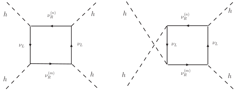
Figure 1: Diagrams that dominantly contribute to ${\rm Im}({\cal A})$.

Before detailing the full calculation, we present an order of magnitude estimate of ${\rm Im}({\cal A})$. Due to the unitarity of the ${\rm S}$-matrix, ${\rm Im}({\cal A})$ is given by the sum of the cut diagrams. We obtain an estimate by ignoring the KK masses in the intermediate state, and furthermore, by using the continuum approximation, c.f. Eq. (11). We define $N_{s}$ so that the highest KK state accessible to the cut diagram is given by $\frac{N_{s}}{R}=\sqrt{s}$, and we get

$${\rm Im}({\cal A}) \sim \frac{1}{16\pi}\sum_{nm}^{N_{s}}\left(\frac{m_{\nu}}{v}\right)^{4}\left(S_{\delta-1}|n|^{\delta-1}\right)\left(S_{\delta-1}|m|^{\delta-1}\right)\ ,$$ (39)

$$\sim \frac{1}{16\pi}\left(\frac{m_{\nu}}{v}\right)^{4}\frac{1}{2}\;\left(\frac{S_{\delta-1}}{\delta}\right)^{2}N_{s}^{2\delta}$$

$$\sim \frac{1}{32\pi}\left(\frac{m_{\nu}}{v}\right)^{4}\left(\frac{S_{\delta-1}}{\delta}\right)^{2}(\sqrt{s}R)^{2\delta}\ .$$

We see from this estimate that the amplitude can grow quite steeply, especially for larger $\delta$, and the suppression due to the small coupling $m_{\nu}/v$ can be overcome by the growth in the number of states. Thus, for the theory to be unitary up to $\sqrt{s}\approx M_{*}$, Eq. (37) implies a lower bound on $1/R$.

We have performed a detailed calculation by taking into account the KK masses. We perform a change of variables to write $n$ in terms of $m^{(n)}$, c.f. Eqs. (22) and (II.2) and use the continuum approximation to convert the double sum in Eq. (38) into a double integral to get

$${\rm Im}({\mathcal{A}})=\frac{1}{16\pi}S^{2}_{\delta-1}R^{2\delta}\int^{\sqrt{s}}_{0}\!{\rm d}m^{(n)}\int^{\sqrt{s}-m^{(n)}}_{0}\!{\rm d}m^{(m)}\left[m^{(n)}{m^{(m)}}\right]^{\delta-1}{\rm Im}({\mathcal{M}}^{(nm)}).$$ (40)

We use FeynCalc Feyncalc to calculate ${\mathcal{M}}^{(nm)}$, and we get

$${\mathcal{M}^{(nm)}} = \left(\frac{m_{\nu}}{v}\right)^{4}\pi^{2}\Biggl{\{}4B_{0}(s,m^{(m)\,2},m^{(n)\,2})+2B_{0}(t,m^{2}_{\nu},m^{2}_{\nu})+2B_{0}(u,m^{2}_{\nu},m^{2}_{\nu})$$

$$~{}~{}~{}~{}+f^{c}_{1}(s)\,\,C_{0}(m^{2}_{h},m^{2}_{h},s,m^{(m)\,2},m^{2}_{\nu},m^{(n)\,2})$$

$$~{}~{}~{}~{}+\biggl{[}f^{c}_{2}(t)\,\,C_{0}(m^{2}_{h},m^{2}_{h},t,m^{2}_{\nu},m^{(m)\,2},m^{2}_{\nu})+(t\rightarrow u)\biggl{]}$$

$$~{}~{}~{}~{}+\biggl{[}f^{c}_{3}(t)\,\,C_{0}(m^{2}_{\nu},m^{2}_{h},t,m^{2}_{\nu},m^{(n)\,2},m^{2}_{\nu})+(t\rightarrow u)\biggl{]}$$

$$~{}~{}~{}~{}+\biggl{[}f^{d}(t)\,\,D_{0}(m^{2}_{h},m^{2}_{h},m^{2}_{h},m^{2}_{h},s,t,m^{(m)\,2},m^{2}_{\nu},m^{(n)\,2},m^{2}_{\nu})+(t\rightarrow u)\biggl{]}\Biggl{\}},$$

where $B_{0}$, $C_{0}$ and $D_{0}$ are the Passarino-Veltman (PV) scalar functions Passarino:1978jh , and $f^{c}_{1}$, $f^{c}_{2}$, $f^{c}_{3}$ and $f^{d}$ are defined as

$$f^{c}_{1}(s) = 4\left(s+2m^{2}_{\nu}+2m^{(m)}m_{\nu}+2m^{(n)}m_{\nu}+2m^{(m)}m^{(n)}-2m^{2}_{h}\right),$$ (42)

$$f^{c}_{2}(t) = t+2m^{(m)\,2}+4m_{\nu}m^{(m)}+2m^{2}_{\nu}-2m^{2}_{h},$$

$$f^{c}_{3}(t) = t+2m^{(n)\,2}+\,4m_{\nu}m^{(n)}+2m^{2}_{\nu}-2m^{2}_{h},$$

$$f^{d}(t) = t\left((m^{(m)}-m^{(n)})^{2}-s\right)+2\left((m^{(m)}+m_{\nu})^{2}-m^{2}_{h}\right)\left((m^{(n)}+m_{\nu})^{2}-m^{2}_{h}\right).$$

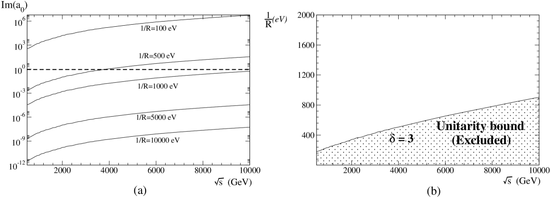
Figure 2: Unitarity bounds for $\delta=3$. The theory is unitary if the solid line in (a) corresponding to the given $1/R$ does not cross the dotted line (${\rm Im}(a_{0})=1$) at a $\sqrt{s}$ less than $M_{*}$. The unitarity constraint on the 1/R vs. $\sqrt{s}$ plane is shown in (b).

The functions $f^{c}_{1}$, $f^{c}_{2}$, $f^{c}_{3}$ and $f^{d}$ are all real, and therefore, ${\rm Im}({\mathcal{M}}^{(nm)})$ is given by the imaginary parts of the PV scalar functions. We present the calculation of the imaginary parts of the PV functions $B_{0}$, $C_{0}$, $D_{0}$, in Appendix B. To obtain ${\rm Im}({\mathcal{A}})$, we then perform a Monte-Carlo integration of Eq. (40) over $m^{(n)}$ and $m^{(m)}$, and expand it into partial waves using Eq. (35). We show the resulting ${\rm Im}(a_{0})$ in Fig. 2(a) for $\delta=3$, as a function of $\sqrt{s}$ for different choices of $1/R$ (from $10^{2}$ eV to $10^{4}$ eV). For $\delta=3$, the region in $1/R$ vs. $\sqrt{s}$ that satisfies the unitarity bound, c.f. Eq. (37), is shown in Fig. 2(b). We infer from these plots that for $\delta=3$ and $\sqrt{s}=1$ TeV, we require $1/R>250$ eV, for unitarity not to be violated.

Using the bound just obtained for $\delta=3$, we can use Eq. (39) to estimate the bounds for $\delta=1,2$. For $\delta=2$ and $\sqrt{s}=1$ TeV, we find the unitarity bound, $1/R>10^{-3}$ eV. For $\delta=1$, we find that the unitarity bound is very weak.

V Conclusions

The Standard Model (SM) of high energy physics suffers from the gauge hierarchy problem, which is the fine tuning required to maintain a low electroweak scale ($M_{EW}\sim 10^{3}$ GeV) in the presence of another seemingly fundamental scale, the Planck scale (the scale of gravity, $M_{pl}\sim 10^{19}$ GeV). Theories with $n$ large extra dimensions have the potential to address the hierarchy problem as shown by Arkani-Hamed, Dimopoulos and Dvali (ADD) Arkani-Hamed:1998rs ; Antoniadis:1998ig .

Recent neutrino oscillation experiments Fukuda:1998mi ; Ahmad:2002ka ; Wolfenstein:1977ue ; Bahcall:2002hv have suggested a small non-zero mass for the neutrino. It has been shown Dienes:1998sb ; Arkani-Hamed:1998vp ; Dvali:1999cn that if right-handed bulk neutrinos (SM gauge singlets) propagate in $\delta$ of these large extra dimensions ($\delta\leq n$), then the smallness of the neutrino mass can be explained.

We considered such bulk neutrinos in the ADD framework where the fundamental scale in nature is postulated to be $M_{*}\sim 1$ TeV. Theories with $\delta\geq 2$ naturally give the right order of neutrino masses with the coefficient of the Yukawa interaction for the neutrino being $O(1)$. However, for $\delta=1$, with the requirement that oscillation constraints be satisfied, this coefficient has to be $O(10^{-5})$, c.f. Table 1, making the theory unnatural.

We performed the Kaluza-Klein (KK) expansion of the bulk neutrino field to obtain the equivalent four dimensional theory starting from a $4+\delta$ dimensional theory. It is common in the literature to analyze theories with $\delta=1,2$, while in this paper we considered $\delta=1,2,3$. However, in the case of $\delta>2$, we find, as expected, for some observables the sum over KK states can be divergent. We took an effective theory approach and cut the KK sum off at $M_{*}$, where we expect new physics to regulate this divergence.

We take the view, as others have Davoudiasl:2002fq , that the standard three-active-flavor analysis explains the neutrino oscillation data. (We do not address the LSND result.) This seems highly plausible given the Super-Kamiokande and the SNO neutral current data. Thus the oscillation into sterile KK neutrino states must be constrained to be smaller than the current precision in experimental data.

Using the KK theory, we estimated the probability of the three active neutrino species to mix into sterile KK neutrino states. This probability is constrained by experiments such as CHOOZ and fits to the atmospheric oscillation data, leading to bounds on the radius ($R$) of extra dimensions that right-handed neutrinos propagate in. We have compiled the bounds on $1/R$ for $\delta=1,2,3$ in Table. 2, showing a strong bound for $\delta=3$. For example, in the normal hierarchy of neutrino masses, we find $1/R$ has to be bigger than about $0.15,1.5,5600$ eV for $\delta=1,2,3$ respectively. We also present bounds for the inverted and the degenerate mass schemes. The mixing probability is divergent when summed over the KK states for $\delta\geq 2$, with a mild logarithmic dependence on the physics that comes in at $M_{*}$ for $\delta=2$, and a stronger linear dependence in the case of $\delta=3$. We do not predict the bounds for $\delta>3$, since the dependence on the high energy completion of the extra dimensional theory we are working with would be increasingly stronger for bigger $\delta$. Our bounds have an additional source of uncertainty from using the continuum approximation rather than performing a discrete sum over the KK states.

We also present bounds on $1/R$ coming from maintaining perturbative unitarity in the theory, in the Higgs-Higgs scattering channel. The bound is due to the growth in the large number of KK states that contribute in the intermediate state as the collision energy increases. The unitarity bound is also quite strong, especially for $\delta=3$, as shown in Fig. 2, albeit not as strong as the bound derived from oscillation data.

It is interesting to ask what signatures of bulk neutrinos there might be at a high energy collider. Since the only coupling to SM fields of the bulk neutrino is through the Yukawa coupling, one promising channel is the production of the KK states in the final state in association with the Higgs. Even though the coupling of the Higgs to the neutrino is much suppressed, the rate can be enhanced to measurable levels owing to the large number of KK states that can be produced in the final state. This is the subject of our forthcoming paper.

Acknowledgments

We thank H.-J. He, H.K. Kim, T. Tait, K. Tobe and J. Wells for useful discussions. This work was supported in part by the NSF grants PHY-0244919 and PHY-0100677.

Appendix A 2-component diagonalization

We can arrive at the mass eigenvalues obtained in Sec. II.2, using two component Weyl fields and putting the neutrino mass matrix in a symmetric form. This is achieved by making the field definitions Dienes:1998sb ,

$$N^{(\hat{n})}\equiv\frac{1}{\sqrt{2}}\left(\nu_{R}^{(\hat{n})}+\nu_{L}^{(\hat{n})}\right),\ \ \ M^{(\hat{n})}\equiv\frac{1}{\sqrt{2}}\left(\nu_{R}^{(\hat{n})}-\nu_{L}^{(\hat{n})}\right).$$ (43)

We can then rewrite Eq. (9) as,

$${\cal L}^{(4)}=-\frac{1}{2}\frac{|\hat{n}|}{R}\left[N^{(\hat{n})}N^{(\hat{n})}-M^{(\hat{n})}M^{(\hat{n})}+h.c.\right]-\frac{m_{\nu}}{v}h\left[\nu_{R}\nu_{L}+\sum_{\hat{n}}\left(N^{(\hat{n})}\nu_{L}+M^{(\hat{n})}\nu_{L}\right)+h.c.\right].$$ (44)

Defining $\nu^{T}=(\nu_{L}\ \nu_{R}\ N^{(1)}\ M^{(1)}\ .\ .\ .\ N^{(N)}\ M^{(N)})$ and with $\left<h\right>=v$, we get the neutrino mass term,

$${\cal L}^{(4)}_{\rm mass}=\frac{1}{2}\left[\nu^{T}~{}{\cal M}~{}\nu+h.c.\right]$$ (45)

where the neutrino mass matrix ${\cal M}$ is given by,

$${\cal M}=\pmatrix{0&m_{\nu}&m_{\nu}&m_{\nu}&.&.&m_{\nu}&m_{\nu}&.&.&.&.\cr m_{\nu}&0&&&&&&&&&&\cr m_{\nu}&&\frac{1}{R}&&&&&&&&&\cr m_{\nu}&&&-\frac{1}{R}&&&&&&&&\cr.&&&&.&&&&&&&\cr.&&&&&.&&&&&&\cr m_{\nu}&&&&&&\left(\frac{|\hat{n}|}{R}\right)_{d_{\hat{n}}\times d_{\hat{n}}}&&&&&\cr m_{\nu}&&&&&&&\left(-\frac{|\hat{n}|}{R}\right)_{d_{\hat{n}}\times d_{\hat{n}}}&&&&\cr.&&&&&&&&.&&&\cr.&&&&&&&&&.&&\cr.&&&&&&&&&&\frac{N}{R}&\cr.&&&&&&&&&&&-\frac{N}{R}}.$$ (46)

The alternating sign on the diagonal reflects the Dirac nature of masses. We have already noted that for $\delta>1$, the state with mass $\pm\frac{|\hat{n}|}{R}$ at the ${\hat{n}}^{\rm th}$ level has a degeneracy $d_{\hat{n}}$.

The characteristic equation, ${\rm Det}({\cal M}-\lambda~{}{\mathbf{1}})=0$ is,

$$\left[\prod_{|\hat{n}|=1}^{N}\left(|\hat{n}|^{2}-(\lambda R)^{2}\right)^{d_{\hat{n}}}\right]\left[(\lambda R)^{2}-(m_{\nu}R)^{2}+2(\lambda R)^{2}(m_{\nu}R)^{2}\sum_{|\hat{k}|=1}^{N}\frac{d_{\hat{k}}}{|\hat{k}|^{2}-(\lambda R)^{2}}\right]=0.$$ (47)

where, $k$ similar to $n$, is shorthand for $(k_{1},...,k_{\delta})$. In order to respect neutrino oscillation experimental bounds, we have to restrict ourselves to $m_{\nu}R\equiv\xi\ll 1$, and in the analysis that follows, we will keep terms only up to $O(\xi^{2})$.

The lightest neutrino mass given by the lowest eigenvalue of Eq. (47), in the limit $2\xi^{2}\sum_{\hat{n}}\frac{d_{\hat{n}}}{|\hat{n}|^{2}}\ll 1$, is

$$m^{(0)}\approx\pm m_{\nu}(1-\xi^{2}\sum_{\hat{n}}\frac{d_{\hat{n}}}{|\hat{n}|^{2}}).$$ (48)

The heavier masses are as follows:
For $\delta=1$, we have $d_{n}=1$ for all $n$ and this case was considered in Ref. Dienes:1998sb . For the KK level with $d_{n}=1$, in Eq. (47), $\lambda R=n$ is never a solution, and only the second of the two factors in square brackets is relevant. We find the eigenvalue $\lambda_{n}R=\pm n(1+\xi^{2}+\xi^{4})$ and the corresponding eigenvector,

$$e_{n(1)}^{\pm}=\frac{1}{\sqrt{\cal N}_{n}}\pmatrix{1&\frac{m}{\pm\lambda_{n}}&.&.&.&\frac{m}{(\pm\lambda_{n}-k/R)}&\frac{m}{(\pm\lambda_{n}+k/R)}&.&.&.}^{T}\ ,$$ (49)

where the superscript $T$ on the row vector represents the transpose operation, and the reciprocal of the normalization constants are,

$$\frac{1}{{\cal N}_{0}}=\frac{1}{2}\left[1-2\xi^{2}\sum_{\hat{n}}\frac{d_{\hat{n}}}{\hat{n}^{2}}\right]\ ,\ \ \ \ \ \frac{1}{{\cal N}_{\hat{n}}}=\xi_{\hat{n}}^{2}d_{\hat{n}}.$$

However, at the $n^{\rm th}$ KK level, if $d_{n}>1$ we can infer from Eq. (47) that there are two classes of eigenstates:

• one with eigenvalue $\pm\frac{|n|}{R}\left[1+(\xi^{2}+\xi^{4})d_{n}\right]$ with eigenvector as shown in Eq. (49),

• $(d_{n}-1)$ states with eigenvalues $\pm\frac{|n|}{R}$ and the corresponding eigenvectors having the first $2n$ entries zero, and with the structure,

  $$e_{n(2,...,d_{n})}^{\pm}=\pmatrix{0&.&.&0&v_{1}&.&.&v_{2d_{n}}&0&.&.&0}^{T}\ .$$ (50)

The eigenvalues found here agree with Eqs. (22) and (II.2).

The matrix $V$ that diagonalizes the mass matrix Eq. (46) have the $e_{n}$ as columns. Neutrino oscillation from an active state to a sterile state computed using this matrix $V$ agrees with that found using Eq. (20).

Appendix B Imaginary part of Passarino-Veltman functions

The unitarity of the $S-$matrix requires that twice of the imaginary part of any scattering amplitude can be written as

$$2{\rm Im}\mathcal{M}(a\rightarrow b)=\sum_{f}\int d\Pi_{f}\mathcal{M}^{*}(b\rightarrow f)\mathcal{M}(a\rightarrow f),$$ (51)

in which the sum $\sum_{f}$ runs over all possible final-state $f$, and $\Pi_{f}$ represents the phase space of final-state $f$. We use the Cutkosky cutting rules to calculate the imaginary part of the Passarino-Veltman scalar functions $B_{0},C_{0},D_{0}$ which were encountered in Sec. IV.

The Feynman diagrams ($\mathcal{M}_{i}$) and the corresponding cut diagrams ($\mathcal{M}_{i}^{\prime}$), which are related with each other as in Eq. (51), are shown in the upper and lower parts of Fig. 3, respectively. The label $i=2,3,4$ represents the two-point, three-point and four-point diagrams, respectively. In general the N-point one-loop scalar integral in $D-$dimension is

$$T_{N}(p_{1},\cdots,p_{N-1},m_{0},\cdots,m_{N-1})=\frac{(2\pi\mu)^{4-D}}{i\pi}\int{\rm d}^{D}q\frac{1}{\mathcal{D}_{0}\mathcal{D}_{1}\cdots\mathcal{D}_{N-1}},$$ (52)

with the denominator factors

$$\mathcal{D}_{0}=q^{2}-m_{0}^{2},\qquad\mathcal{D}_{i}=(q+p_{i})^{2}-m_{i}^{2},\qquad{\rm with}\;\;i=1,\cdots,N-1,$$

originating from the propagators in the Feynman diagram. The $i\epsilon$ part of the denominator factors is suppressed. Here we adapt the conventions of Ref. Denner:kt .

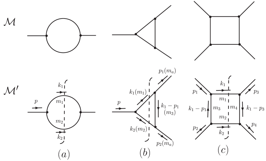
Figure 3: Feynman diagrams of scalar functions and the corresponding cut diagrams.

B.1 Two-point integrals, $B_{0}$ function

The scalar two-point diagram ($\mathcal{M}_{2}$) in Fig. 3(a) is given by

$$\mathcal{M}_{2}=\int\frac{{\rm d}^{4}q}{(2\pi)^{4}}\frac{1}{\mathcal{D}_{0}\mathcal{D}_{1}}=\frac{1}{16\pi^{2}}B_{0}(p^{2},m_{1}^{2},m_{2}^{2}),$$

from which we obtain the imaginary part of $B_{0}$, by applying the Cutkosky rules, as

$${\rm Im}(B_{0}) = 8\pi^{2}\times 2\,{\rm Im(\mathcal{M}_{2})}$$ (53)

$$= 8\pi^{2}\times\mathcal{M}_{2}^{\prime}$$

$$= 2\,\int\frac{{\rm d}k_{1}}{2E_{1}}\frac{{\rm d}k_{2}}{2E_{2}}\delta^{4}(k_{1}+k_{2}-p)$$

$$= \pi\beta^{*},$$

where $\beta^{*}$ is defined as

$$\beta^{*}=\frac{1}{p^{2}}\sqrt{\left(p^{2}-(m_{1}+m_{2})^{2}\right)\left(p^{2}-(m_{1}-m_{2})^{2}\right)}.$$

B.2 Three-point integrals, $C_{0}$ function

The scalar three-point diagram ($\mathcal{M}_{3}$) in Fig. 3(b) is given by

$$\mathcal{M}_{3}=\int\frac{{\rm d}^{4}q}{(2\pi)^{4}}\frac{1}{\mathcal{D}_{0}\mathcal{D}_{1}\mathcal{D}_{2}}=\frac{1}{16\pi^{2}}C_{0}(p_{1}^{2},p_{2}^{2},s,m_{1}^{2},m_{3}^{2},m_{2}^{2}),$$

from which we obtain the imaginary part of $C_{0}$ function as

$${\rm Im}(C_{0}) = 8\pi^{2}\times\mathcal{M}_{3}^{\prime}$$

$$= \frac{1}{4}\beta^{*}\int{\rm d}\Omega^{*}\frac{1}{(k_{1}-p_{1})^{2}-m_{3}^{2}}.$$

In the c.m. frame, with the scattering angles $\theta,\phi,\theta^{*},\phi^{*}$ defined in Fig. 4, the $4-$momenta is

$$p_{1} = \frac{\sqrt{s}}{2}(1,\beta\sin\theta,0,\beta\cos\theta),$$

$$p_{2} = \frac{\sqrt{s}}{2}(1,-\beta\sin\theta,0,-\beta\cos\theta),$$

$$k_{1} = \frac{\sqrt{s}}{2}(\hat{E_{1}},\beta^{*}\sin\theta^{*}\cos\phi^{*},\beta^{*}\sin\theta^{*}\sin\phi^{*},\beta^{*}\cos\theta^{*}),$$

$$k_{2} = \frac{\sqrt{s}}{2}(\hat{E_{2}},-\beta^{*}\sin\theta^{*}\cos\phi^{*},-\beta^{*}\sin\theta^{*}\sin\phi^{*},-\beta^{*}\cos\theta^{*}),$$ (54)

with $s=p^{2}=(p_{1}+p_{2})^{2}$, $p_{1}^{2}=p_{2}^{2}=m_{a}^{2},$ $k_{1}^{2}=m_{1}^{2}$, $k_{2}^{2}=m_{2}^{2}$ and

$$\beta = \sqrt{1-\frac{4m_{a}^{2}}{s}},$$

$$\beta^{*} = \frac{\sqrt{\left(s-(m_{1}+m_{2})^{2}\right)\left(s-(m_{1}-m_{2})^{2}\right)}}{s},$$

$$\hat{E_{1}} = \frac{s+m_{1}^{2}-m_{2}^{2}}{s},$$

$$\hat{E_{2}} = \frac{s+m_{2}^{2}-m_{1}^{2}}{s}.$$ (55)

After a straightforward calculation, we find the imaginary part of $C_{0}$ to be

$${\rm Im}(C_{0})=\frac{\pi\beta^{*}}{p^{2}}\,\frac{1}{\beta\beta^{*}}\,\ln\frac{f+\beta\beta^{*}}{f-\beta\beta^{*}}$$ (56)

where $f$ is defined as

$$f=\frac{s-m_{1}^{2}-m_{2}^{2}-2m_{a}^{2}+2m_{3}^{2}}{s}.$$

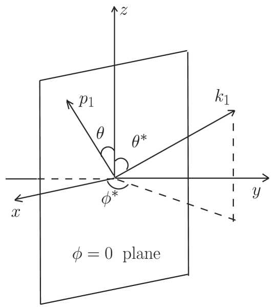
Figure 4: Kinematics of the cut diagrams

B.3 Four-point integrals, $D_{0}$ function

The scalar four-point diagram ($\mathcal{M}_{4}$) in Fig. 3(c) is given by

$$\mathcal{M}_{4}=\int\frac{{\rm d}^{4}q}{(2\pi)^{4}}\frac{1}{\mathcal{D}_{0}\mathcal{D}_{1}\mathcal{D}_{2}\mathcal{D}_{3}}=\frac{1}{16\pi^{2}}D_{0}(p_{1}^{2},p_{2}^{2},p_{3}^{2},p_{4}^{2},s,t,m_{1}^{2},m_{3}^{2},m_{2}^{2},m_{4}^{2}),$$

from which we obtain the imaginary part of $D_{0}$ function as

$${\rm Im}(D_{0}) = 8\pi^{2}\times\mathcal{M}_{4}^{\prime}$$

$$= \frac{1}{4}\beta^{*}\int{\rm d}\Omega^{*}\frac{1}{(k_{1}-p_{1})^{2}-m_{3}^{4}}\,\frac{1}{(k_{1}-p_{3})^{2}-m_{4}^{2}}.$$

Using the same kinematics defined in Eqs. (54) and (55),

$${\rm Im}(D_{0})=\left\{\begin{array}[]{l}\displaystyle\frac{2\pi\beta^{*}}{s^{2}}\;\frac{1}{\sqrt{K}}\;\ln\Biggl{[}\frac{(BP-2AQ)(Px+Q)+2K-2P\sqrt{K(Ax^{2}+Bx+C)}}{Px+Q}\Biggl{]}\Biggl{|}^{x=1}_{x=-1}\\[8.53581pt] \hskip 312.9803pt({\rm for}\;K>0),\\[19.91692pt] \displaystyle\frac{2\pi\beta^{*}}{s^{2}}\;\frac{1}{\sqrt{-K}}\;\arcsin\Biggl{[}\frac{2K+(BP-2AQ)(Px+Q)}{P(Px+Q)\sqrt{B^{2}-4AC}}\Biggl{]}\Biggl{|}^{x=1}_{x=-1}\hskip 22.76228pt({\rm for}K<0),\\[19.91692pt] \displaystyle-\frac{2\pi\beta^{*}}{s^{2}}\;\Biggl{[}\frac{2P\;\sqrt{Ax^{2}+Bx+C}}{(BP-2AQ)(Px+Q)}\Biggl{]}\Biggl{|}^{x=1}_{x=-1}\hskip 113.81102pt({\rm for}\;K=0),\par\end{array}\right.$$ (61)

where the variables $A$, $B$, $C$, $P$, $Q$ and $K$ are defined to be

$$A=\beta^{2}{\beta^{*}}^{2},$$ (62)

$$B=-2f\beta\beta^{*}\cos\theta,$$

$$C=f^{2}-\beta^{2}{\beta^{*}}^{2}\sin^{2}\theta,$$

$$P=\beta\beta^{*},$$

$$Q=-f,$$

$$K=AQ^{2}-BPQ+CP^{2},$$

and $f$ is defined as

$$f=\frac{s-m_{1}^{2}-m_{2}^{2}-2m_{a}^{2}+2m_{3}^{2}}{s}.$$

References

- (1) Y. Fukuda et al. [Super-Kamiokande Collaboration], Phys. Rev. Lett. 81, 1562 (1998) [hep-ex/9807003]; M. B. Smy et al. [Super-Kamiokande Collaboration], [hep-ex/0309011].
- (2) Q. R. Ahmad et al. [SNO Collaboration], Phys. Rev. Lett. 89, 011302 (2002) [nucl-ex/0204009]; A. L. Hallin et al., Nucl. Phys. Proc. Suppl. 118, 3 (2003);
- (3) L. Wolfenstein, Phys. Rev. D 17, 2369 (1978); S. P. Mikheev and A. Y. Smirnov, Sov. J. Nucl. Phys. 42, 913 (1985) [Yad. Fiz. 42, 1441 (1985)].
- (4) J. N. Bahcall, M. C. Gonzalez-Garcia and C. Pena-Garay, JHEP 0207, 054 (2002) [hep-ph/0204314]; M. C. Gonzalez-Garcia and C. Pena-Garay, Phys. Rev. D 68, 093003 (2003) [hep-ph/0306001].
- (5) A. Aguilar et al. [LSND Collaboration], Phys. Rev. D 64, 112007 (2001) [hep-ex/0104049].
- (6) N. Arkani-Hamed, S. Dimopoulos and G. Dvali, Phys. Lett. B 429, 263 (1998) [hep-ph/9803315].
- (7) I. Antoniadis, N. Arkani-Hamed, S. Dimopoulos and G. R. Dvali, Phys. Lett. B 436 (1998) 257 [hep-ph/9804398].
- (8) K. R. Dienes, E. Dudas and T. Gherghetta, Nucl. Phys. B 557, 25 (1999) [hep-ph/9811428].
- (9) N. Arkani-Hamed, S. Dimopoulos, G. R. Dvali and J. March-Russell, Phys. Rev. D 65, 024032 (2002) [hep-ph/9811448].
- (10) G. R. Dvali and A. Y. Smirnov, Nucl. Phys. B 563, 63 (1999) [hep-ph/9904211].
- (11) R. N. Mohapatra, S. Nandi and A. Perez-Lorenzana, Phys. Lett. B 466, 115 (1999) [hep-ph/9907520]; R. N. Mohapatra and A. Perez-Lorenzana, Nucl. Phys. B 576, 466 (2000) [hep-ph/9910474]; R. N. Mohapatra and A. Perez-Lorenzana, Nucl. Phys. B 593, 451 (2001) [hep-ph/0006278]; K. R. Dienes and I. Sarcevic, Phys. Lett. B 500, 133 (2001) [hep-ph/0008144]; C. S. Lam and J. N. Ng, Phys. Rev. D 64, 113006 (2001) [hep-ph/0104129].
- (12) H. Davoudiasl, P. Langacker and M. Perelstein, Phys. Rev. D 65, 105015 (2002) [hep-ph/0201128].
- (13) A. Ioannisian and A. Pilaftsis, Phys. Rev. D 62, 066001 (2000) [hep-ph/9907522]; R. Barbieri, P. Creminelli and A. Strumia, Nucl. Phys. B 585, 28 (2000) [hep-ph/0002199]; G. C. McLaughlin and J. N. Ng, Phys. Rev. D 63, 053002 (2001) [nucl-th/0003023]; Phys. Lett. B 493, 88 (2000) [hep-ph/0008209]; K. Abazajian, G. M. Fuller and M. Patel, Phys. Rev. Lett. 90, 061301 (2003) [hep-ph/0011048]; H. S. Goh and R. N. Mohapatra, Phys. Rev. D 65, 085018 (2002) [hep-ph/0110161]; G. Cacciapaglia, M. Cirelli and A. Romanino, Phys. Rev. D 68, 033013 (2003) [hep-ph/0302246].
- (14) A. De Gouvea, G. F. Giudice, A. Strumia and K. Tobe, Nucl. Phys. B 623, 395 (2002) [hep-ph/0107156].
- (15) G. F. Giudice, R. Rattazzi and J. D. Wells, Nucl. Phys. B 544, 3 (1999) [hep-ph/9811291].
- (16) Z. Maki, M. Nakagawa and S. Sakata, Prog. Theor. Phys. 28, 870 (1962).
- (17) M. Apollonio et al. [CHOOZ Collaboration], Phys. Lett. B 466, 415 (1999) [hep-ex/9907037].
- (18) B. Kayser, Phys. Rev. D 24, 110 (1981).
- (19) K. Hagiwara et al. [Particle Data Group Collaboration], Phys. Rev. D 66, 010001 (2002).
- (20) A. D. Dolgov, Phys. Rept. 370, 333 (2002) [hep-ph/0202122]; S. M. Bilenky, C. Giunti, J. A. Grifols and E. Masso, Phys. Rept. 379, 69 (2003) [hep-ph/0211462].
- (21) M. Bando, T. Kugo, T. Noguchi and K. Yoshioka, Phys. Rev. Lett. 83, 3601 (1999) [hep-ph/9906549]; T. Kugo and K. Yoshioka, Nucl. Phys. B 594, 301 (2001) [hep-ph/9912496]; H. Murayama and J. D. Wells, Phys. Rev. D 65, 056011 (2002) [hep-ph/0109004].
- (22) R. Mertig, M. Bohm, and A. Denner, Comp. Phys. Comm. 64, 345(1991).
- (23) G. Passarino and M. J. G. Veltman, Nucl. Phys. B 160, 151 (1979); G. ’t Hooft and M. J. G. Veltman, Nucl. Phys. B 153, 365 (1979).
- (24) A. Denner, Fortsch. Phys. 41, 307 (1993).