Abstract

We trace here instantons through the analysis of pure Yang-Mills gluon Green functions in the Landau gauge for a window of IR momenta ($0.4$ GeV $<k<0.9$ GeV). We present lattice results that can be fitted only after substituting the BPST profile in the Instanton liquid model (ILM) by one based on the Diakonov and Petrov variational methods. This also leads us to gain information on the parameters of ILM.

1 Introduction

An appealing approach to analytically understand some of the non-perturbative features of QCD is the evaluation of quantum fluctuations around topologically non-trivial classical solutions through the expansion of the path integral around these solutions. In fact these considerations are often generalized to configurations which are not exact solutions of the field equations but close to them and which we will name quasi-classical field configurations.

Famous examples of non-trivial solutions of classical equations of motion are instantons [1, 2]. Quasi-classical solutions considered in instanton liquid models [3, 4] provide a successful connection between the instanton zero modes and the QCD chiral symmetry breaking (See ref. [5] for a good review on the subject).

More recently, it has been proven in ref. [6] that instanton model predictions for quark-quark interaction agree with non-perturbative QCD lattice results better than those from Schwinger-Dyson (SD) models with a perturbative structure of the QCD interaction (vector quark-gluon coupling parametrization). In general, a dominance of instanton-induced effects on the dynamics of the QCD light-quark sector seems to emerge, although it is not excluded that SD models with pseudo-scalar and scalar quark-gluon couplings might capture this emerging instanton physics. On the other hand, despite instantons have been first considered as a possible explanation of confinement [7], it is now generally accepted that they do not generate the area law for Wilson loops .

We have recently argued [8] that instantons, or instanton-like structures, have dramatic effects on the low momentum Green function in Yang-Mills theories and that they can explain the observed $\propto k^{4}$ behaviour of the non-perturbative MOM QCD coupling constant computed on the lattice. Notice that this remark, not only advocates in favor of the presence of these quasi-classical structures in the lattice gauge configurations, but also indicates that the quantum fluctuations do not contribute significantly to the Green functions in this momentum regime. In the present paper we try a low momentum description of two- and three-gluon Green functions through Instanton liquid model (ILM).

The succesful description of the MOM QCD coupling constant in the low-momentum regime is based on the sum-ansatz approach, that builds the classical solution as a linear combination of modified instantons. Although instanton profile modifications play no role in obtaining the coupling constant, at least in the first approximation, any description of two- and three-gluon Green functions makes mandatory to further elaborate on the nature of this modifications. To this goal we will follow the Diakonov & Petrov (DP) sum-ansatz approach [4]. As will be discussed later, different aspects of this approach have been criticised by Shuryak and Verbaarshot, but it provides us with a framework able to estimate instanton effects through analytical or semi-analytical computations which seem to work reasonably well. This is the “phenomenological” point of view which we adopt in this paper to extract some understanding of the low-momentum behaviour of lattice Green functions.

The paper is organized in six sections. In section 2 we discuss the pattern of the running with momenta of the QCD coupling constant. Section 3 is devoted to study the instanton profile modification within the DP approach. In section 4, we show that the low momentum behaviour of lattice gluon Green functions is rather well described by ILM only after including instanton profile modifications and discuss how the large instanton density obtained from the fits is expected to be reduced by light dynamical quarks in full QCD. In section 5, the effect of instanton radius distribution is discussed. We finally conclude in section 6.

At the end of the day, of course, rather important questions still remain open: why do quantum effects appear to be suppressed in this low momentum range ? Has this some connection with confinement ?

2 The QCD coupling constant: four regimes

We have presented in Ref. [8] a preliminary claim of instanton dominance at low energy by analyzing in Landau gauge the following ratio of pure Yang-Mills Green functions:

$$\alpha_{s}(k^{2})\ =\ \frac{1}{4\pi}\left(\frac{G^{(3)}(k^{2},k^{2},k^{2})}{(G^{(2)}(k^{2}))^{3}}Z_{\rm MOM}^{3/2}(k^{2})\right)^{2}\ =\frac{k^{6}}{4\pi}\ \frac{\left(G^{(3)}(k^{2},k^{2},k^{2})\right)^{2}}{\left(G^{(2)}(k^{2})\right)^{3}},$$ (1)

which is a non-perturbative MOM definition of the coupling constant, where $G^{(n)}$ is the gluon n-point correlation function and $Z_{\rm MOM}=k^{2}G^{(2)}$ is the gluon propagator renormalization constant in MOM scheme .

In Fig. 1 we show on a log-log plot, that a roughly-$k^{4}$ power law is satisfied by the lattice evaluations of $\alpha_{s}(k^{2})$, eq. (1), up to 0.8-0.9 GeV, for three different lattices, strongly supporting a quasi-classical description [8].

A very striking feature of the results shown in Fig. 1, obtained with a low statistics of 20 configurations, is that there is a rather sharp transition at $\sim 1{\rm GeV}$ between two regimes: below this scale $\alpha_{s}(k^{2})$ does not seem to fluctuate much, it agrees well, with a small $\chi^{2}$, with the expected $k^{4}$ linear behaviour in spite of the small statistics and it complies with an instanton-like picture, while above that scale the data suddenly deviate from the $k^{4}$ law and become apparently fuzzier , a fuzziness which is confirmed by the larger $\chi^{2}$ which affects any smooth fit. A tempting interpretation is that this fuzziness has to do with a strong influence of quantum fluctuations which increase suddenly above 1 GeV. We may understand this as follows: for a given profile and a given instanton radius, the ILM predicts no statistical fluctuation of the Green functions. The average over the instantons locations and their color orientation does not create any noise on Green functions which are translational and color rotation invariant. Only the dispersion (to be studied at length in this paper) of the instanton radius as well as varying effects of the neighbouring instantons produces some statistical noise. On the contrary the quantum contributions to Green function are generated by statistical fluctuations of the gauge fields around zero and Green functions appear as correlations in this statistical system. Some confirmation of this interpretation results of the analysis of the same gluon Green functions after applying a cooling procedure that kills short-distance (quantum) correlations [11].

Altogether we may distinguish four regimes:

• Above 2.6 GeV we have shown [12, 13] that the lattice data were dominated by perturbative QCD with a significant non-perturbative correction describable via OPE by the expectation value of $A^{2}$. This means clearly a dominance of quantum fluctuations with small corrections from the $A^{2}$ condensate which may be generated by the quasi-classical solutions. Indeed the quasi-classical solutions, being large structures, are seen by the hard propagating gluons as an effectively translational invariant background. It is then easy to show that their dominant effect is amenable to an OPE treatment of the lowest dimension operator: $A^{2}$ [14].

• Between $\sim$ 0.4 and $\sim$ 0.9 GeV the quasi-classical contributions dominate and the quantum effects are strongly depressed.

• The 1.0 to 2.6 GeV region shows a strong quantum effect. However, it is not at all describable in terms of perturbation theory. A description in terms of quantum fluctuations in a quasi-classical background should be tried. The latter background can no longer be treated as simply as in the large momentum regime. Other non-perturbative effects may also play a role, for example related to confinement.

• The very low momentum region below $\sim 0.4$ GeV is still “terra incognita” and, being of the order of $2\pi/L$, ($L$ being the lattice length) possibly strongly sensitive to finite volume artifacts.

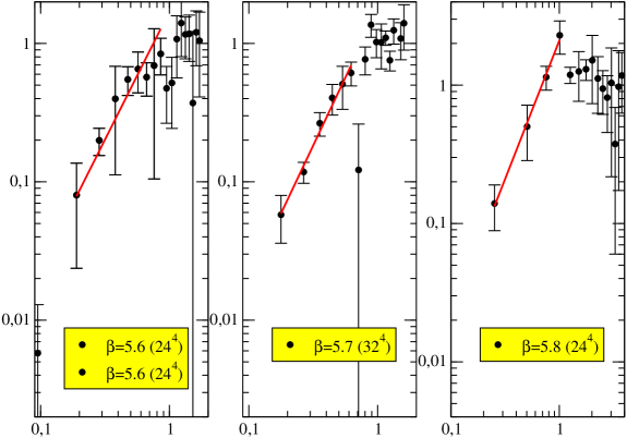
Figure 1: The low momentum $k^{4}$ behavior of $\alpha_{s}(k^{2})$ on log-log plots for three different lattices ((5.6,24), (5.7,32), (5.8,24)) using 20 configurations. Notice that above $\sim 1$ GeV, no smooth line can be easily drawn joining the lattice data.

3 A modified profile for the instanton-liquid model

In the following, we will try to describe the Green functions assuming that the relevant quasi-classical solutions are instanton liquids. Let us compute the quantity in eq. (1). We describe gluon fields in the low energy regime as a superposition of modified instantons, a quasi-classical background dominance being assumed. In this framework, the gauge field in Landau gauge will be given by:

$$g\,B_{\mu}^{a}({\bf x})=2\sum_{i}R^{a\alpha}_{(i)}\,\overline{\eta}^{\alpha}_{\mu\nu}\frac{(x_{\nu}-z_{\nu}^{i})}{(x-z^{i})^{2}}\phi\left(\frac{|x-z^{i}|}{\rho_{i}}\right)\ ,$$ (2)

where $z^{i}$ ($\rho_{i}$) are the center (radius) of the instantons, $\overline{\eta}^{\alpha}_{\mu\nu}$ is known as ’t Hooft symbol, $R^{a\,\alpha}_{(i)}$ are color rotations embedding the canonical $SU(2)$ instanton into the $SU(3)$ gauge group, $\alpha=1,3$ ($a=1,8$) is an $SU(2)$ ($SU(3)$) color index, and the sum is extended over instantons and anti-instantons.

The classical solution for an isolated instanton is the standard BPST one, $\phi(\xi)=1/(\xi^{2}+1)$ [1]. Nevertheless, the superposition (2) with a BPST profile is not a solution of Yang-Mills equations (since they are not linear). Hence, we will discuss below a parameterization of the profile function inspired by an approximated minimization of the action for a finite density of instantons .

Then, just by assuming random color orientation and instanton position , from eq. (2) we obtain (see [8]):

$$g^{2}G^{(2)}_{(I)}(k^{2})=\frac{n}{8}<\rho^{6}I(k\rho)^{2}>$$

$$g^{3}G^{(3)}_{(I)}(k^{2},k^{2},k^{2})=\frac{n}{48\,k}<\rho^{9}I(k\rho)^{3}>$$ (3)

where $n$ stands for the instanton density, $<\cdots>$ denotes average over the instanton radius for a given radius distribution $\mu(\rho)$, normalized to 1, and where

$$I(s)\ =\frac{8\pi^{2}}{s}\int_{0}^{\infty}\ zdzJ_{2}(sz)\,\phi(z)\ ,\ \ \ \ s>0\ ;$$ (4)

$J_{2}$ being the second order Bessel J function. The factor $g^{n}$ for n-points Green functions in l.h.s. of eq. (3) comes from the factor $g$ in the l.h.s. of eq. (2).

Then, from Eq. (1) we get:

$$\alpha_{s\,(I)}(k)\ =\ \frac{k^{4}}{18\pi n}\ \frac{<\rho^{9}I(k\rho)^{3}>^{2}}{<\rho^{6}I(k\rho)^{2}>^{3}}\ .$$ (5)

As a first approximation, if we consider all instantons to have the same radius, we obviously obtain:

$$\frac{<\rho^{9}I(k\rho)^{3}>^{2}}{<\rho^{6}I(k\rho)^{2}>^{3}}\ =\ 1\ ,$$ (6)

and recover an exact $k^{4}$-power law for any instanton profile.

In (6) the influence of the profile will only appear as a sub-leading contribution, that will also depend on the instanton radius distribution (See section 5.), while in (3) the leading contributions to the Green functions depend on the profile and will therefore be used by us to gain some understanding about the instanton radial shape and radii. Indeed, it will be manifest (see fig. 3) that the BPST profile cannot account for the low momentum behaviour of Green functions.

The variational Diakonov & Petrov equation.

If the QCD vacuum can be understood as an instanton liquid of finite density (See [5], for example), the BPST profile will no longer be valid (it is only a zero density limit) especially at large distance from the instanton center where the overlap of neighboring instantons becomes important. Being interested in the low momentum regime we cannot neglect these effects.

A possible method to include the effect of instanton interactions, is to study the profile that minimizes the action of the instanton ensemble. Such a procedure was used in [4], where, through the Feynman variational principle, the equation

$$-\left(x^{2}\frac{d}{dx^{2}}\right)^{2}\phi+\left(1+\frac{\alpha_{\rm DP}^{2}x^{2}}{4}\right)\phi-3\phi^{2}+2\phi^{3}+\frac{x^{2}}{6\beta(\rho)}\frac{\delta C_{N_{C}}}{\delta\phi}=0\ ,$$

(7)

was obtained for the best profile, $\phi$, eq. (6.7) in [4] . In the last term $\beta(\rho)=8\pi^{2}/g^{2}(\rho)$ where $g(\rho)$ is the running coupling constant evaluated at the instanton radius scale and $C_{N_{C}}$ is a factor containing the quantum corrections that multiply the instanton liquid partition function and are basically defined by the functional determinants in eq. (2.19) of [4].The value of $\alpha_{\rm DP}$ which represents an average classical effect of the other instantons on one of them is given by

$$\alpha_{\rm DP}^{2}=\frac{4}{3}\gamma_{0}^{2}n\frac{\beta(\overline{\rho})}{\beta(\rho)}<\int_{0}^{\infty}dx^{2}\phi^{2}\left(\frac{x}{\rho}\right)>\ .$$ (8)

where the parameter $\gamma_{0}$ is related to the instanton interaction strength,

$$\gamma_{0}^{2}\ =\ \frac{27N_{c}\pi^{2}}{4(N_{c}^{2}-1)}\ .$$ (9)

Thus, if we assume the same radius for all the instantons, this equation reduces to

$$\alpha_{\rm DP}^{2}\simeq\frac{9N_{c}\pi^{2}}{N_{c}^{2}-1}n\int_{0}^{\infty}dx^{2}\phi^{2}\left(\frac{x}{\rho}\right)\ .$$ (10)

The last term in eq. (7), involving a functional derivative of the functional determinants, is hard to compute and explicitely violates scale invariance (in the sense that $\phi(\frac{x}{a})$ is still a solution if n is divided by $a^{4}$). Let us remark that this is true only if we do not take into account the $\rho$ dependance of $\alpha_{\rm DP}$ due to $\beta(\rho)$.

Now assuming that $\alpha_{\rm DP}$ is approximately constant, it is argued in [4] (discussion before eq. (6.1)) that one can neglect this term to get a scale invariant equation governing the large distance shape of the profile function assumed to be dominated by classical interaction. Of course, we should borrow from the neglected term some scale invariance breaking to fix the instanton size and match to the BPST solution at small distances. This can be done e.g. by explicitely writing the profile as a function of $|x|/\rho$, $\rho$ defining the instanton size through the condition $\phi(1)=1/2$.

The term in $\alpha_{\rm DP}$ enforces a squeezing of the instantons and therefore controls the large $x$ behaviour of $\phi(x)$. For $|x|\gg\rho$ we can neglect in Eq. (7) the non linear terms obtaining the following Bessel equation:

$$\left\{x^{2}\frac{d^{2}}{d|x|^{2}}+|x|\frac{d}{d|x|}-\left(4+\alpha_{\rm DP}^{2}x^{2}\right)\ \right\}\ \phi\left(\frac{|x|}{\rho}\right)\ =\ 0\ .$$ (11)

Therefore we have:

$$\phi\left(\frac{|x|}{\rho}\right)\begin{array}[]{c}\rule[5.69046pt]{0.0pt}{14.22636pt}\sim\\ x\gg\rho\end{array}c\ K_{2}(\alpha_{\rm DP}|x|)\ \ \sim\ \ c\ \frac{e^{-\alpha_{\rm DP}|x|}}{\sqrt{|x|}}\ ,$$ (14)

where c is an unknown coefficient which could be determined from the scale invariance breaking condition. Let us make further remarks about Eq. (7) after neglecting the $C_{N_{C}}$ term: the authors of  [4] claim that at small x the term proportional to $\alpha^{2}_{\rm DP}x^{2}$ becomes small and therefore can be neglected, recovering the instanton equation. This term is nevertheless not negligeable wih respect to $\phi-3\phi^{2}+2\phi^{3}$ which tends to 0 when $x\to 0$. Furthermore this equation has no solution going to 0 at infinity and to 1 at $x=0$ because a singularity emerges at some small finite value of $x$.

For the above reasons, we prefere to use in the next sections instead of direct solutions of eq. (11) the following parametrization:

$$\phi\left(\frac{|x|}{\rho}\right)=\frac{(\alpha_{\rm DP}\rho)^{2}}{2}\ \frac{K_{2}(\alpha_{\rm DP}x)}{1+\displaystyle\frac{(\alpha_{\rm DP}\rho)^{2}}{2}K_{2}(\alpha_{\rm DP}x)}\ ,$$ (15)

that behaves as $K_{2}(\alpha_{\rm DP}|x|)$ at $x\gg\rho$  and at short distances as:

$$\phi\left(\frac{|x|}{\rho}\right)=\frac{\rho^{2}}{\rho^{2}+x^{2}}+O(\alpha_{\rm DP}x)\ ,$$ (16)

where for $\alpha_{\rm DP}\,x\ll 1$ we indeed recover the BPST instanton. Remember that the zero $\alpha_{\rm DP}$ limit is also, from eq. (10), the zero density limit. Notice that the imposed constraint, expressed by eq. (16), of a behaviour a la BPST at $\alpha_{\rm DP}\,x\ll 1$ is de facto the scale invariance breaking condition in our approach. It differs slightly from DP’s proposal $\phi(1)=1/2$ since $\phi(1)=1/2-(\alpha_{\rm DP}\rho)^{2}/16+O((\alpha_{\rm DP}\rho)4)$. For the values of $\alpha_{\rm DP}$ and ${\overline{\rho}}$ which we will use to fit the lattice data both are in practice equivalent. We show in fig. 2 a plot of this profile for $x/\rho>1/2$ compared to a numerical solution of Eq. (7) equal to $1/2$ at $x/\rho=1$ and going to $0$ at infinity (for $\alpha_{\rm DP}\rho=0.675$). In the following, we will consider eq. (15) as our optimal choice for the profile function.

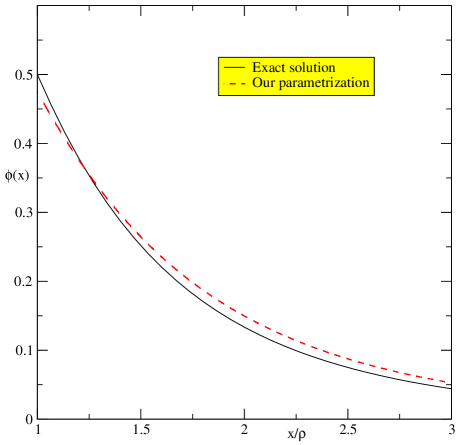
Figure 2: Comparison between our parametrization of the profile function wit $\alpha_{DP}\rho=0.68$ and the exact solution of the Diakonov and Petrov equation.

4 Green functions

The goal of this section is to apply the parameterization in eq. (15) to fit our numerical results, obtaining thus $\rho$, $\alpha_{\rm DP}$ and the instanton density. We start by writing the gauge field as the addition of a classical part, $B_{\mu}^{a}({\bf x})$, and a quantum one, $Q_{B}({\bf x})$, depending in general on the classical background:

$$A_{\mu}^{a}({\bf x})=B_{\mu}^{a}({\bf x})+{(Q_{B})}_{\mu}^{a}({\bf x})\ ,$$ (17)

then, for the two-point gluon Green function, we can write :

$$\langle A_{\mu}^{a}({\bf 0})A_{\nu}^{b}({\bf x})\rangle=\langle B_{\mu}^{a}({\bf 0})B_{\nu}^{b}({\bf x})\rangle\ +\langle(Q_{B})_{\mu}^{a}({\bf 0})(Q_{B})_{\nu}^{b}({\bf x})\rangle\ ,$$ (18)

or after Fourier transformation,

$$G^{(2)}_{\rm lattice}(k^{2})=G^{(2)}_{(I)}(k^{2})\ +\ G^{(2)}_{Q}(k^{2})\ .$$ (19)

The working hypothesis we derive from the interpretation of fig. 1, is that in a certain region of momenta, say below $\sim$ 1 GeV, quantum effects are strongly suppressed and only classical properties are seen. Of course, we introduce this hypothesis based on a phenomenological observation, but it is not unconceivable that an intrinsically non-perturbative phenomenon like confinement could cause the disappearance of quantum correlations at distances larger than the confining scale.

4.1 Estimated corrections to the instanton liquid model

From our data we have been led to fit the bare Green functions to the r.h.s of eq. (3) in a range $k_{\rm min}<k<k_{\rm max}$ without any correction. It is far from obvious that we can neglect either quantum corrections or lattice truncations of the quasi-classical model. This subsection is devoted to justify our choice. For the sake of clarity, we will pay the price of anticipating on the results of some fits which will be later detailed.

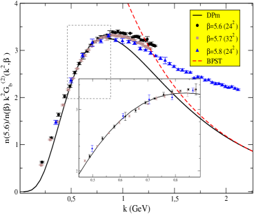
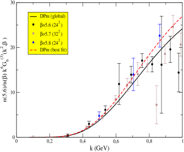
(a)	(b)

Figure 3: (a) We plot the gluon propagator, $k^{2}G^{(2)}$, for the three lattices after a rescaling that matches data from $\beta=5.7$ and $\beta=5.8$ to those from $\beta=5.6$. The dotted line is obtained from the BPST profile with $\rho=0.3$ fm and the solid line is the best fit using our profile parameterization for the gluon propagator. BPST cannot manifestly describe lattice data. (b) The points are lattice evaluations of symmetric vertex, $k^{6}G^{(3)}$. The solid line is the best fit for the vertex with our profile parameterization, the density being required to be the same for both propagator and vertex, and the dotted is the best fit with a free density in the fitting.

• The Green functions $G^{(n)}$ estimated from three different lattice spacings match reasonably to each other, after a mere rescaling to a common value for some $k_{\rm max}$ of the order of 1 GeV (see Fig. 3). These matching coefficients are close to 1, approximately in the ratios 0.95 / 1.0/ 1.05 for $\beta=5.6,5.7,5.8$.

• It is difficult to know precisely which mechanism drives these matching coefficients slightly away from 1: quantum corrections, ultraviolet/infrared cutoffs on quasi-classical solutions. It is also impossible to know if these corrections are multiplicative, additive or of a more complex nature. The main lesson is that these corrections are small, and we decide for convenience to describe them by a multiplicative rescaling factor.

• This factor is defined as

  $$\Gamma^{(m)}(k^{2},a^{-1})\ \ =\ \ \frac{G^{(m)}_{\rm lattice}(k^{2},a^{-1})}{G^{(m)}_{(I)}(k^{2})}\ ,$$ (20)

  where $a^{-1}$ is the regularization scale i.e. the inverse lattice spacing and $G^{(m)}_{(I)}(k^{2}),m=2,3$ are given in eq. (3). The functions $\Gamma^{(m)}(k^{2},a^{-1})\,n\,\beta/6$ , $n$ being the instanton density, are plotted up to an unknown global constant in fig. 4(a). $G^{(2)}_{(I)}(k^{2})$ is here the best fit to be discussed later. These plots show the good matching of different lattice spacings after performing a constant multiplicative rescaling (fig 4(b) shows the result of this rescaling). They show a wide parabola having its minimum around $k=0.65$ GeV, this minimum is around 7 to 8 which corresponds to the order of magnitude of the instanton density we will derive (the other factors being close to 1).

  One possible explanation of this parabolic behaviour is an expected increase of quantum corrections towards larger $k$ and, towards lower $k$, a relative increase of the ratio due to the fast decrease of the denominator in eq. (20): for example the fast increase at low $k$ might be due to additive quantum corrections which are only visible when the quasi-classical background is very small. Additive corrections are anyhow necessary at $k=0$ since the lattice data are non vanishing while the denominator of eq. (20) is zero. Whether this non vanishing of the lattice propagator at $k=0$ is a finite volume effect violating Zwanziger’s theorem [17], will not be discussed in this paper since, as already mentioned, we restrain from discussing the finite-volume sensitive region below $\sim 0.4$ GeV.

  
  

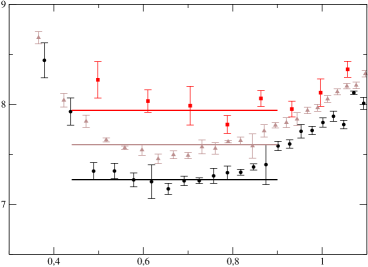
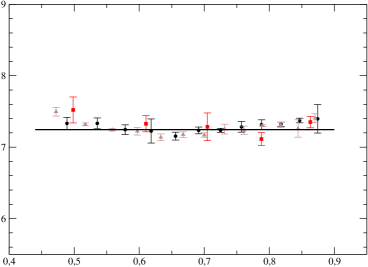
  (a)		(b)

  Figure 4: (a) We plot the ratios $n\,\Gamma^{(2)}(k^{2},a^{-2})\beta/6$ where $n$ is the instanton density and $\Gamma^{(2)}$ defined in eq. (20), for the three lattices, the squares, triangles and circles corresponding respectiveley to $\beta=5.8$, $\beta=5.7$ and $\beta=5.6$. The horizontal axis represents the momentum in GeV. (b) The same points as in (a) but with the multiplicative rescaling performed. Different $\beta^{\prime}s$ coincide quite well, all show a parabolic type dependence in $k$.

• If we stick to the momentum range plotted in fig. 4(b) these ratios do not deviate from a constant by more than a few percent. We will therefore perform our fits only in this range $k_{\rm min}-k_{\rm max}$  and approximate $\Gamma^{(2)}(k^{2},a^{-1})$ by a constant:

  $$\Gamma^{(2)}(k^{2},a^{-1})\begin{array}[]{c}\rule[0.0pt]{0.0pt}{22.76228pt}\sim\rule[0.0pt]{14.22636pt}{0.0pt}\\ k_{\rm min}^{2}\raise 1.29167pt\hbox{$<$\kern-7.5pt\raise-4.73611pt\hbox{$\sim$}}k^{2}\raise 1.29167pt\hbox{$<$\kern-7.5pt\raise-4.73611pt\hbox{$\sim$}}k_{\rm max}^{2}\end{array}\Gamma^{(2)}(a^{-1})\ ,$$ (23)

• Since from fig. 4(a) the different $\Gamma^{(2)}(a^{-1})$ differ also by no more than a few percent we decide to take from now on all these $\Gamma^{(2)}(a^{-1})$’s as equal at the cost of an expected discrepancy between the fitted densities of a few percent. We take

  $$\forall a^{-1},\quad\Gamma^{(2)}(a^{-1})\ \ =\ \Gamma^{(2)}\left(a^{-1}(5.6)\right)\ .$$ (24)

  where $a^{-1}(5.6)$ is the inverse lattice spacing for $\beta=5.6$.

• We now wonder if the hypothesis eq.(24) can be extended to the coefficients $\Gamma^{(3)}(a^{-1})$. The small dependence on $k$ and on $a^{-1}$ can be seen, although with larger errors, in fig. 3(b) where the different lattice data seem to fit one common solid curve representing the model. The next question is the validity of the hypothesis

  $$\Gamma^{(3)}(a^{-1})\ \ =\Gamma^{(2)}(a^{-1}).$$ (25)

  To test the hypothesis $\Gamma^{(3)}\sim\Gamma^{(2)}$ we can look at fig. 5. The vertical axis corresponds to the ratio $\Gamma^{(3)}(a^{-1}(5.6)/\Gamma^{(2)}(a^{-1}(5.6))$ or equivalently to $n^{(3)}/n^{(2)}$ where we define $n^{(m)}\equiv n\Gamma^{(m)}(a^{-1}(5.6))$, $n$ being the instanton density. The horizontal axis corresponds to the instanton radius $\rho$, supposed to be the same for all instantons. For that instanton radius a best fit of the bare Green functions is performed according to the formula:

  $$G^{(m)}_{\rm lattice}(k^{2},a^{-1})=G^{(m)}_{(I)}(k^{2})\ \Gamma^{(m)}(a^{-1}(5.6))$$ (26)

  with $G^{(m)}_{(I)}(k^{2})$ given by eq. (3). The plot 5 shows for each $\rho$ an agreement between different $\beta$’s which is a surprise: it tells that the ratio $\Gamma^{(3)}(a^{-1})/\Gamma^{(2)}(a^{-1})$ is almost independent of the lattice spacing even though it does strongly depend on $\rho$. The dotted curve shows the $\chi^{2}$ of the common fit to $G^{(2)}$ and $G^{(3)}$. The smallest $\chi^{2}$ corresponds to a ratio $\Gamma^{(3)}(a^{-1})/\Gamma^{(2)}(a^{-1})$ ranging from 0.8 to 0.9, i.e. close to 1. This also corresponds to a value of the radius around 0.3 fm which is the one favored by phenomenology. This leads us to consider eq. (25) as quite reasonable.

• All the arguments up to now have shown an approximate equality to a few percent of all $\Gamma^{(m)}(a^{-1})$’s. We are left with an unknown global constant. The fact that these factors are so close to each other suggests that the corrections to the instantonic contribution (whatever their origin may be) are small. It is then natural to expect that these correction factors are also close to 1. This is confirmed by a result which will be detailed at the end of this paper via the following argument: if we initially take $\Gamma^{(2,3)}\neq 1$, apply MOM renormalisation and then eq. (1), we obtain:

  $$\alpha_{\rm Latt}(k)\ =\ \frac{k^{6}}{4\pi}\frac{\left(G_{\rm Latt}^{(3)}(k^{2},a_{\rm Latt}^{-1})\right)^{2}}{\left(G_{\rm Latt}^{(2)}(k^{2},a_{\rm Latt}^{-1})\right)^{3}}\ =\underbrace{\frac{\left(\Gamma^{(3)}(a_{\rm Latt}^{-1})\right)^{2}}{\left(\Gamma^{(2)}(a_{\rm Latt}^{-1})\right)^{3}}}\ \ \alpha_{(I)}(k)$$ (27)

  where the term above the curly bracket in the r.h.s. introduces a supposed-to-be-sub-leading correction, depending on the regularization parameter, that we neglect in our analysis for the present work (and did the same in [8]). Let us anticipate some of our next results: the reasonable agreement between the instanton density obtained from the coupling constant $\alpha_{\rm Latt}(k)$ in table 3 with the one in table 1 implies a ratio $(\Gamma^{(3)})^{2}/(\Gamma^{(2)})^{3}$ close to 1. The latter, combined with $\Gamma^{(2)}/\Gamma^{(3)}\sim 1$ presented in the preceding item, ends up with an approximate justification of our hypothesis that all $\Gamma^{(n)}(a^{-1}),n=2,3\sim 1$ for all $\beta$’s in the range considered here.

Thus, our final working hypothesis is:

$$\Gamma^{(m)}(k^{2},a^{-1})=1\quad{\rm for\ \ m=2,3\ \ and}\quad k_{\rm min}<k<k_{\rm max}.$$ (28)

with $k_{\rm min}=0.44$ GeV and $k_{\rm max}=0.89$ GeV.

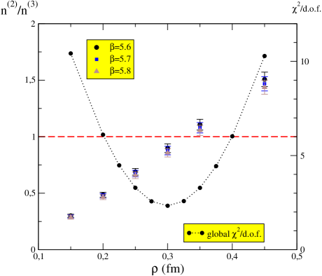
Figure 5: We plot the ratios $n^{(3)}/n^{(2)}$ where we define $n^{(m)}\equiv n\Gamma^{(m)}(a^{-1}(5.6)$, $n$ being the instanton density. These are fitted from two-point and three-point Green functions for a fixed value of instanton radius, $\rho$, represented on the horizontal axis. The dotted line joins the optimal $\chi^{2}/d.o.f.$ (on left y-axis) as a function of the radius.

4.2 Numerical results.

The numerical data that we shall exploit systematicaly all over the paper result from two simulations on a $24^{4}$ lattice with bare coupling constants given by $\beta=5.6$ and $\beta=5.8$, and a simulation on a $32^{4}$ lattice for $\beta=5.7$, in the Landau gauge. The gluon correlations functions are obtained from only 20 field configurations, that are enough to manifest the classical background effects we search for. However, more field configurations are available for some of the lattices and we used them to check that those exploited are not particularly biased. We calibrate all these simulations with the ratios of lattice spacings for different $\beta$’s given in ref. [18] and $a_{\rm Latt}^{-1}(\beta=6.0)=1.97$ GeV (this last value was used in ref. [19] consistently with the very precise measurement of the lattice spacing resulting from a non-perturbatively improved action in ref. [20]).

Coefficients in [18] are fitted for $\beta=6/g^{2}\geq 6$. In this work, we make use of rather low values $\beta<6.0$, in order to have larger volumes. These low values of $\beta$ show for the quantity $\alpha_{s}$ a good scaling with results at $\beta\geq 6.0$, a signal that these lower $\beta$’s provide reasonable results. The risk with these simulations is the extrapolation needed to calibrate the lattice spacing, that might be a non-negligible source of systematic error in our measures.

$\rho$ (fm)	0.2	0.25	0.3	0.35	0.4
$\beta=5.6$	26.5(1)	13.18(5)	7.75(3)	5.12(2)	3.63(1)
n   $\beta=5.7$	27.2(1)	13.54(5)	7.98(3)	5.28(3)	3.76(2)
(fm-4) $\beta=5.8$	27.8(2)	13.9(1)	8.20(7)	5.41(4)	3.86(3)
$\alpha_{\rm DP}\rho$	0.393(2)	0.527(2)	0.675(2)	0.836(3)	1.005(3)
$\chi^{2}/d.o.f.$	6.1	3.3	2.3	3.3	6.0

Table 1: Best-fit parameters for several fixed instantons radii. The two- and three-point Green functions are fitted simultaneously with the some instanton density. Note that the stated errors are only statistical.

We collect the results of our fits for several fixed instanton radii in tab. 1. An instanton density, although the same for both Green functions , is independently fitted for each particular lattice spacing. We look thus for a remnant of a sub-leading dependence on the regularization parameter. The careful reader may have noticed that the relative density splitting between different $\beta$’s is slightly smaller (3 % for $\delta\beta=0.1$) than the splitting between the linear fits in fig. 4 (4.5 %). This is due the factor $g^{2}$ in eq. (3) (about 1.5 %).

Crudeness of our quasi-classical approximation.

It is worth to insist that our fit rely on the crude approximation given by eq. (28) which is not valid beyond a few percents as discussed at length in subsection 4.1. This is the origin of the difference between the densities in tab. 1. This is also the reason why the minimal $\chi^{2}/d.o.f.$ in table 1 is of the order of two because we force the overall factor to be the same in fits for both two- and three-point Green functions. This tells about the crudeness of completely neglecting the sub-leading contributions from quantum fluctuations and lattice truncation of the classical solutions. Much better matchings might have been obtained had we relaxed the constraint eq. (28). We refrained from doing so because it would have needed additional input about quantum fluctuations and lattice truncation of classical solutions which would have been mere guesses and would not have yielded any stronger evidence.

At the present stage of the work, the best we can do is to assume eq. (28) and get what we believe to be a fairly coherent description of our whole set of lattice data. The best-fit parameterization in Tab. 1 is the best we can achieve, and it is not that bad, although we know that the density obtained there is affected roughly by a 20% of systematic uncertainty.

4.3 QCD versus pure gluon-dynamics

Our measured densities in tab. 2, while in the ballpark of lattice estimations, give a contribution to the gluon condensate $\left\langle{g^{2}{G_{\mu\nu}^{a}}^{2}}\right\rangle\sim 4{\rm GeV}^{4}\sim(1400\ {\rm MeV})^{4}$ for $n\sim 8\,{\rm fm}^{-4}$, significantly larger than other estimates, based on QCD sum rules [30], $\left\langle{g^{2}{G_{\mu\nu}^{a}}^{2}}\right\rangle\sim 0.5\ {\rm GeV}^{4}\sim(840{\rm MeV})^{4}$, or more recently [31], $\left\langle{g^{2}{G_{\mu\nu}^{a}}^{2}}\right\rangle\sim 0.9{\rm GeV}^{4}\sim(970{\rm MeV})^{4}$. A significant difference between the pure Yang-Mills condensate and the one from QCD sum rules is however expected: in ref. [32] (see eq. (106) ) it is argued that light dynamical quarks might reduce the $G^{2}$ condensate by a factor 2 to 3. In fact, it can be argued that the low eigenvalues of the fermion determinant reduce the instanton contribution from the action and hence the resulting instanton density. In addition, some re-shaping of instanton profiles for a strongly correlated vacuum populated by fermions cannot be discarded. As a result, estimates in pure gluon-dynamics should differ substantially from those in QCD and only the analysis of unquenched ($N_{f}\neq 0$) lattices simulations of gauge fields could help us to quantify this discrepancy.

Not only the same analysis of this paper for unquenched simulations could quantify the discrepancy, but we may also appeal to the connection of $A^{2}$-condensate and the ILM approach: the gluon condensate of dimension two can be computed by extracting the momentum power OPE correction to the perturbative formula of Landau-gauge Green functions from their lattice estimates above $\sim 2.6$ GeV (see discusion in section 2) [12]. This condensate is to be computed at a given renormalization point, $\mu_{0}$, lying on the momentun range of OPE-dominance.

Now, if we run the renormalization point $\mu_{0}$ of the $A^{2}$-condensate down to some instanton scale, $\mu_{I}$, with the help of the one-loop renormalisation goup equations (RGE), we obtain [14]:

$$\langle A^{2}_{\rm inst}\rangle\equiv 12\pi\rho^{2}n\simeq\langle A^{2}_{R,\mu_{I}}\rangle\simeq\langle A^{2}_{R,\mu_{0}}\rangle\left(1+\frac{35}{44}\ \frac{\ln{(\mu_{I}/\mu_{0})}}{\ln{(\mu_{0}/\Lambda_{\rm QCD})}}\right)\ ;$$ (29)

where we match the OPE+RGE estimate to an ILM semiclassical one. Of course, the latter is a purely semiclassical estimate deprived of the UV-fluctuations around the classical minima which we assume to be subleading at the appropriated instanton scales (see again the discussion in section 2). Thus, the instanton density can be roughly estimated from the dimension-two gluon-condensate.

Although the gluon condensate for quenched simulations has been largely studied [12] in literature, unfortunatly only a very preliminar analysis of the MOM QCD coupling constant from a lattice simulation with two dynamical-quark flavours is available [13]. Furthermore, this analysis is performed for such high quark masses that no effect of instanton suppression is to be expected and indeed no significant effect has yet been seen. Progress in the unquenched determination of the gluon condensate will be, of course, welcome.

Moreover, the QCD sum rules are not so accurate and neither are our density estimates which, for instance, would be modified by the presence of other “instanton-like structures” or instantons deformations.

Altogether our density estimate is close to the maximum acceptable: with a density of 8 per fm⁴ the average distance between two neighbouring instanton centers is of the order of 0.6 fm i.e. twice the average radius, a really dense packing.

5 The effect of the instanton radius dispersion

We have performed satisfactory and independent fits for the three different lattices from $\alpha_{s}$ to the $k^{4}$-formula, eqs. (5, 6), and obtain the estimates for the instanton density shown in the second column of Tab. 2. They differ by about a 30 % from the profile dependent ones obtained from $G^{(m)}$ and presented in table 1. The fit of $\alpha_{s}$ is done on a rather firm ground since, contrarily to the fits of $G^{(m)}$, the prediction does not at all depend on the profile neither on the radius but only on eq.(6), of course on the hypothesis that the radius distribution is a delta function i.e. that all the radii are equal. $\alpha_{s}$ is therefore the best quantity to estimate the corrections to this rather drastic hypothesis. If the $k^{4}$ law does not depend on the instanton profiles but only on the $\delta$-function distribution, the corrections do .

First, we face the problem of computing the corrections to the previous $\delta$-function result from a more general optics: we just consider some small width for the distribution, $\delta\rho$, and compute in perturbations of $\delta\rho/\overline{\rho}$ around the average radius, $\overline{\rho}$. We can write:

$$<\rho^{3m}I^{m}(k\rho)>\ =\ I^{m}(k\overline{\rho})\ <\rho^{3m}>\ +\ \frac{d}{d\rho}I^{m}(k\overline{\rho})\ <\rho^{3m}(\rho-\overline{\rho})>$$

$$+\ \frac{1}{2}\frac{d^{2}}{d\rho^{2}}I^{m}(k\overline{\rho})\ <\rho^{3m}(\rho-\overline{\rho})^{2}>\ +\dots\ .$$ (30)

we take $\rho=\overline{\rho}+\delta\rho$ , assume the distribution to be symmetric (at least for small perturbations) around the peak, i.e. $<\delta\rho>=0$ and then obtain:

$$<(\overline{\rho}+\delta\rho)^{n}>\ =\ \overline{\rho}^{n}\left(1+\frac{n(n-1)}{2}\ \frac{\delta\rho^{2}}{\overline{\rho}^{2}}+{\cal O}\left(\frac{\delta\rho^{4}}{\overline{\rho}^{4}}\right)\right)\ ,$$

$$<(\overline{\rho}+\delta\rho)^{n}\delta\rho>\ =\ n\overline{\rho}^{n+1}\frac{\delta\rho^{2}}{\overline{\rho}^{2}}\ +{\cal O}\left(\frac{\delta\rho^{4}}{\overline{\rho}^{4}}\right)\ ,$$

$$<(\overline{\rho}+\delta\rho)^{n}\delta\rho^{2}>\ =\ \overline{\rho}^{n+2}\ \frac{\delta\rho^{2}}{\overline{\rho}^{2}}\ +{\cal O}\left(\frac{\delta\rho^{4}}{\overline{\rho}^{4}}\right)\ .$$ (31)

Thus, we derive for the QCD MOM coupling constant defined in eq. (1) the following expression:

$$\alpha(k)\ =\ \frac{k^{4}}{18\pi n}\ \left(1\ +\ \frac{\delta\rho^{2}}{\overline{\rho}^{2}}\ \left(12+12\overline{\rho}f(k\overline{\rho})+3\overline{\rho}^{2}f^{2}(k\overline{\rho})\right)+{\cal O}\left(\frac{\delta\rho^{4}}{\overline{\rho}^{4}}\right)\right)\ ,$$ (32)

where all the dependence on the profile function comes through the function $f$ defined as

$$f(k\overline{\rho})\ =\ \left.\frac{d}{d\rho}\ln\int_{0}^{\infty}zdzJ_{2}(k\rho z)\phi(z)\ \ \right|_{\rho=\overline{\rho}}\ .$$ (33)

In particular, for the BPST profile, we find:

$$\overline{\rho}f(k\overline{\rho})\ =\ -2\ \frac{1-\displaystyle\frac{k^{3}\overline{\rho}^{3}}{8}\left(K_{1}(k\overline{\rho})+K_{3}(k\overline{\rho})\right)}{1-\displaystyle\frac{k^{2}\overline{\rho}^{2}}{2}K_{2}(k\overline{\rho})}\ .$$ (34)

This function $\overline{\rho}f(k\overline{\rho})$ takes only negatives values for all $k\overline{\rho}$. The same is obtained by applying the DP-inspired profile parametrization defined in eq. (15) (where we take $\alpha\overline{\rho}=0.68$ from the previous section) to eq. (33) and, as can be seen in plot 6, the functions $f$ obtained from both profiles evolve rather close to each other for all $k\overline{\rho}$. This suggests a pattern that eq. (32) obeys in rather general manner: the $k^{4}$-power law is corrected by a positive $k\overline{\rho}$-independent term and by a negative one depending on $k\overline{\rho}$; the first one gives some pre-factor larger than 1 to the $k^{4}$ formula and the second can be numerically simulated rather well over the window $(0.4-0.9)$ GeV by reducing the power on $k$,

$$\alpha(k)\ \simeq\ \frac{c}{18\pi n\overline{\rho}^{4}}\left(k\overline{\rho}\right)^{4-\varepsilon}\ .$$ (35)

This last result, eq. (35), altogether with the constraints $c>1$ and $\varepsilon>0$, are the main and more general result of the section. The values of $\varepsilon$ and $c$ depend on the particular profile and on the width of the radii distribution, as given by eqs. (32,33) in the small width limit.

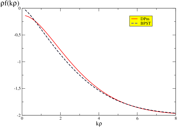
Figure 6: The function $\overline{\rho}f(k\overline{\rho})$ defined in the text in terms of $k\overline{\rho}$ for both DP-inspired and BPST profiles.

We will now proceed as follows. We will first estimate the parameter $\varepsilon$ by fitting our lattice data for MOM QCD coupling constant to the formula eq. (35), where $n/c$ is to be taken as a free parameter to be tuned. Then, we will estimate the width and the instanton density, $n$, with the help of eqs. (32,33), i.e. in the small width approximation. Finally, the consequences of employing more realistic radii distributions will be preliminarily discussed, details being in appendix B.

Lattice results

In this subsection, we first collected in tab. 2 the results for the density obtained through the fit of the MOM QCD coupling constant defined in eq. (1) to the $k^{4}$-power law in eqs. (5,6), for our three lattice data set.

Lattice	n (fm-4)
5.6($24^{4}$)	5.2(6)
5.7($32^{4}$)	6.7(4)
5.8($32^{4}$)	6(1)

Table 2: Results for the density obtained from fitting lattice coupling constant to eqs. (5,6) i.e. assuming a $k^{4}$ behavior. Errors quoted are only statistical and computed by the jackknife method

Then, we include in tab. 3 the results for the best fits of the same QCD coupling constant lattice data to the power law formula of eq. (35).

Lattice	$\displaystyle\frac{n}{c}$ (fm-4)	$\varepsilon$	$\chi^{2}$/d.o.f.
5.6($24^{4}$)	6(2)	0.2(4)	0.068
5.7($32^{4}$)	7(3)	0.1(5)	0.36
5.8($24^{4}$)	5(1)	0.2(6)	0.007

Table 3: The same that in tab. 2 but here fitting to eq. (35) for $\overline{\rho}=1.5$ GeV^-1. The third row shows the $\chi^{2}$/d.o.f. The fitted powers are then lower than 4 but the errors show that the power 4 is not excluded by our fits.

We use for both the same fitting window, $0.44<k<0.89$, used in section 4 to obtain the best profile parameterization. The $\chi^{2}$/d.o.f.’s in tab. 3 are tiny. This may be due to: (i) the strong correlation of our lattice estimates of the coupling for the different momenta, all computed from the same set of gauge field configurations ; (ii) the small number of points in our fitting window (only 3 for $5.8(24^{4})$).

The best-fit parameters computed lattice by lattice in tab. 3 manifest no appreciable systematic deviation. A global fit for the whole set seems thus to be appropriate. The resulting power deduced from a global fit is:

$$3.91\pm 0.45\ \ ,$$ (36)

which is compatible with both the general constraint $\varepsilon>0$ and also with a $k^{4}$-power law. The $\chi^{2}$/d.o.f. is 0.39 for this global fit. In ref. [8], the same global fit was performed using also a few other lattices (we added estimates of $\alpha_{s}$ over smaller volumes and larger $\beta$’s: 5.7(24⁴), 5.9(24⁴), 6.0(24⁴,16⁴); these, having only one point inside the fitting window, have been discarded from the present work. The result of the latter analysis was 3.82(8) for the fitted power. The error was there clearly underestimated but the evaluations of the coupling constant from larger $\beta$’s do not practically affect the central value. This fact indicates that exploiting the small $\beta$’s used in the present work does not seem to introduce any sizable bias, at least over the low-momentum region, on the determination of $\alpha_{s}$.

Instanton density in the small width approximation

The global fit for the whole set of lattice data yields $\varepsilon\simeq 0.1$ for the central value estimate of that parameter. If we apply the exact result for $f$ in eq. (33) to eq. (32) and use the latter to estimate $\delta\rho$ through its best numerical matching to the power formula eq. (35) with $\varepsilon=0.1$, we will obtain:

$$\frac{\delta\rho^{2}}{\overline{\rho}^{2}}\simeq 0.01\ .$$ (37)

This results implies that

$$c\simeq 1+12\ \frac{\delta\rho^{2}}{\overline{\rho}^{2}}\simeq 1.12\ .$$ (38)

Thus, densities obtained from tab. 3 will be about 10 % larger than those in tab. 2 because of the factor $c$ in front of the power of $k$. If we compute numerically the function $f$ for the DP-inspired profile and follow the same procedure to estimate the width, the parameter $c$ and hence the corrections to the instanton density estimates from the $k^{4}$-law in tab. 2, we will obtain roughly the same results. This could be expected after checking the rather similar behaviours of the function $f$ obtained from both profiles in plot 6. This means consequently that, once some small width distribution is assumed and practically not regarding to the profile, the estimated instanton density is $n\sim 6-8$ fm^-4.

All these estimates are anyhow in the right ballpark as far as different arguments [16] seem to point towards an instanton density of a few fm^-4 ’s.

Discussing about realistic distributions.

After estimating the effects of a small width distribution, we will discuss the consequences of some instanton distributions proposed in the literature.

It is well known that the one-loop tunneling amplitude of classical minima in gauge theories gives the standard growth $\mu(\rho)\sim\rho^{6}$ for instanton radii distribution [2]. The classical interaction of instantons in the background is thought to introduce small-distance repulsion that strongly suppress large instantons and leads to a well-behaved partition function [5]. Applying the Feynman variational principle to a liquid of BPST instantons, Diakonov & Petrov found indeed that this infrared growth is balanced as follows [4]:

$$\mu(\rho)=2\frac{\left(\frac{2}{7}\overline{\rho^{2}}\right)^{-7/2}}{\gamma(7/2)}\ \rho^{6}\exp{\left(-\frac{7\rho^{2}}{\rule[0.0pt]{0.0pt}{11.38092pt}2\overline{\rho^{2}}}\right)}\ ,$$ (39)

where $\overline{\rho^{2}}=\int_{0}^{\infty}d\rho\rho^{2}\mu(\rho)$ and $\gamma(n)=\int_{0}^{\infty}dte^{-t}t^{n-1}$ is the standar Euler’s gamma function and

$$\left(\overline{\rho^{2}}\right)^{2}\ =\ \frac{7}{2n\gamma_{0}^{2}\beta(\overline{\rho})}\ .$$ (40)

A very important remark is that eqs. (8), particularized for BPST profile and using $\beta(\rho)\simeq\beta(\overline{\rho})$, combined with eq. (40), leads to avoid the dependence on the density and to derive a prediction for the previously fitted parameter $\alpha_{\rm DP}\rho$,

$$\alpha_{\rm DP}\sqrt{\overline{\rho^{2}}}\ =\ \sqrt{\frac{14}{3\beta(\overline{\rho})}}\ \simeq 0.6$$ (41)

where we use $\beta(\overline{\rho})\simeq 15$ as in [4]. The agreement of such a prediction with our lattice estimate is remarkably encouraging since, for our non-BPST profile, this relation has been numerically checked and remain approximately valid.

The goal of this section is anyhow to analyze the impact of the corrections to the equal radii approximation that we use to describe the low momentum behaviour of our lattice Green functions. For this purpose, we remark that the distribution given by eq. (39) is rather asymmetric around $\overline{\rho}$, which is in practice usually defined as $\sqrt{\overline{\rho^{2}}}$. Its width, measured as

$$\frac{\delta\rho^{4}}{\overline{\rho}^{4}}\ =\ \frac{\overline{\rho^{4}}-\left(\overline{\rho^{2}}\right)^{2}}{\left(\overline{\rho^{2}}\right)^{2}}\ =\frac{2}{7}\ ,$$ (42)

leads us to conclude that the previous small approximation could have missed some not negligeable correction. This is why we compute in appendix B the Green functions and the MOM QCD coupling constant on the background of an instanton liquid with radii distribution given by eq. (39) and fit the latter to the power formula given by eq. (35). We do it for BPST and DP-inspired profiles and collect the results in tab. 4. As can be learned from the table, the main conclusions of the small width analysis remain unchanged except for the fact that the estimate of the density increases up to $\sim 7-10$ fm^-4 as a consequence of the values of the parameter $c$.

Profile	$c$	$\varepsilon$
DPm	1.55	0.17
BPST	1.52	0.25

Table 4: Values of the parameters $c$ and $\varepsilon$ in eq. (35) obtained in the appendix B for our DP-inspired and BPST profiles.

Furthermore, the instanton radii distribution has to be varied altogehter with the instanton profile and density in the Diakonov & Petrov formalism. These authors found [4]:

$$\mu(\rho)\ \propto\ \frac{\rho^{11\;s(\rho)}}{\rho^{5}}\exp\left(-\beta n<\Gamma(\rho)\rho^{2}>\Gamma(\rho)\rho^{2}\right)\ ,$$ (43)

for the radii distribution of what they call “fremons”, i.e. the pseudo-instantons obeying the profile equation in (3), where $\Gamma(\rho)\rho^{2}=\gamma_{0}\int dx^{2}\phi^{2}(x/\rho)$. $s(\rho)$ is a function on $\rho$ introducing a very small collective correction to the standard power $\rho^{6}$.

Two aspects which have lead Verbaarschot [21] and Shuryak [3, 22] to criticise the DP formalism are visible in the “fremons” radii distribution in eq. (43): (i) the distribution concerns the radius, $\rho$, of one particular instanton immersed in some “bath” of instantons with average radius, $\overline{\rho}$; how does one combine the two scales in the game, $\rho$ and $\overline{\rho}$, to define the instanton scale for $\beta$ ? Why, for instance, use $\beta(\rho)$ instead of $\beta((\overline{\rho}\rho)^{1/2})$ ? (ii) Such an instanton scale is furthermore of the order of 0.3 fm and hence the coupling $g$ in $\beta$ is to be computed out of the perturbative regime!

Any detailed evaluation of the impact of the “fremon” distribution implies answering these questions, in particular knowing the behaviour on $\rho$ of $\beta(\rho)$ and how it modifies the gaussian in eq. (39). However, this is out of the scope of the present work. We adopt here a “phenomenological” point of view: the DP formalism offers a large-distance damping for the profile that properly corrects the low momentum behaviour of Green functions and leads to a satisfactory description of our lattice data. The large-distance behaviour of the profile is governed by the parameter $\alpha_{\rm DP}\rho$ which is rather well estimated when we put $\beta(\overline{\rho})\simeq 15$ in eq. (41) according to [4]. Moreover, had we assumed $\beta(\rho)\simeq\beta(\overline{\rho})$ and $\Gamma(\rho)\simeq 1$ (this is strictely true for the BPST profile) we would recover the distribution in eq. (39).

As a final remark, if we try to compute the instanton density through any of the two eqs. (10,40) by employing our best-fit parameters in the previous section, we will obtain $\sim 2$ fm^-4. Is something still missing in the DP approach? As a matter of fact, the third main aspect criticised by the authors above mentioned [3, 22, 21] is the too strong instanton interaction strength resulting from the DP formalism and it should be noted that a reduction of $\gamma_{0}^{2}$ by a factor three or four would allow all the pieces of the puzzle to match. Thus, our analysis detects somehow this effect pointed out in the above references regarding the instanton-antiinstanton interaction. It remains to investigate whether our results are compatible with those, for instance in  [21], where the Stream-line approach is used (the author found that $\gamma_{0}^{2}$ is about one order of magnitude smaller than the one from DP).

We should recall however our “phenomenological” point of view: does the sum-ansatz of Diakonov & Petrov, after profile variation, take into account the effects included in the Stream-line analysis, except for some effective rescaling of $\gamma_{0}$ ? A preliminar analysis of this question is avanced in appendix C, where we show how one can build the gauge field through the Shuryak’s ratio-ansatz [22], that gives an approximative solution to the Stream-line equation, and match the sum-ansatz with our DP-inspired instanton profile in both near the center of any of the instantons and far from all them. This could explain why the independent-pseudoparticle approach given by the sum-ansatz accounts for the low momentum behaviour of the MOM QCD coupling constant and Green functions. This point, of course, deserves further attention.

In summary, we dedicated this section to analyze the effects of radius dispersion on the $k^{4}$ power-law that the instanton approach predicts for the MOM QCD coupling constant. Within the small width approximation we establish that the two main effects of radius dispersion appears in our fitting window as a reduction of the power of $k$ and as an overall pre-factor larger than 1. In particular, the pre-factor does not depend on the particular profile function and corrects the estimate of the instanton density from the MOM QCD coupling constant that becomes then compatible with those directly obtained from Green functions in the previous section, $\sim 8$ fm^-4. In fact, this instanton-density estimate is rather general and, as far as the low momentum behaviour of Green functions is dominated by the gauge field at large distances, is not only independent of the profile function but neither is affected by the sum-ansatz approach we used. Nothing seems to change by the use of realistic distributions. Futhermore, the analysis of radius dispersion in terms of realistic distributions gives us the possibility of connecting the “dynamical” parameter $\alpha_{\rm DP}\sqrt{\overline{\rho^{2}}}$ with only the instanton coupling throug $\beta$ and leads to an estimate of $\simeq 0.6$ for the former, in remarkable agreement with our fits.

6 Discussions and Conclusions

In a previous paper [8], we had shown a $k^{4}$ dependence of the coupling constant in MOM scheme, which gave us a rather clean indication of the dominance of semiclassical solutions over low energy QCD dynamics, and some indication that these solutions might be instantons.

In order to go further in the understanding of this very remarkable feature, we tried here a direct description of gluon Green functions in this framework. In order to achieve this, contrarily to what happens for the MOM coupling constant, the knowledge of the instanton profile is mandatory. The single-instanton BPST profile clearly fails to describe the low momentum behavior since it predicts a divergent gluon propagator for $k\to 0$ in full contradiction with the lattice results. This is understood as an effect of the deformation of instantons far from their centers due to the influence of other instantons. Indeed, the BPST singularity of the gluon propagator is corrected when effects of instanton interactions are taken into account through a parameterization of the profile derived from variational methods [4], and it leads to a successful description of the low momentum behavior of lattice two- and three-point Green functions (see fig. 3). At this point, we cannot exclude other ”instanton-like structures” as, for example, a significant amount of merons [9, 10] which would of course modify our density estimates.

We fit our lattice data for the Green functions in an instanton liquid model (ILM), below energies of $\sim 0.9$ GeV, and above $\simeq 0.4$ GeV. Below $\simeq 0.4$ GeV we have too few lattice data and furthermore the lattice computed gluon propagator gives a non null value for the $k\to 0$ limit, in contradiction with the expectation of an ILM:

$$G^{(2)}_{(I)}\sim\left\{\begin{array}[]{l}k^{-2}\quad\mbox{\rm for BPST}\\ k^{2}\quad\mbox{\rm for DP}\end{array}\right.$$ (46)

Futhermore, the quantum corrections to the semiclassical solutions should be more visible when the latter vanish . In fact, a signal that instanton approach could be missing some mechanism in the very low momentum regime is the fact that a very recent analysis within the SD approach leads to

$$G^{(2)}_{\rm SD}\sim\left(k^{2}\right)^{2\kappa-1}\ ,$$ (47)

with $\kappa\simeq 0.595$ [24]. An also recent SD-motivated work, based on rather general arguments, points towards $\kappa=1/2$ [25]. Last but not least, this region is expected to be strongly finite-volume sensitive and deserves a special study.

We have discussed the effect of the instanton radius dispersion. We find a subdominant but non negligible influence of the radius dispersion on the coupling constant: We find that a coherent description of both two- and three-point Green functions only emerges when the instanton radius reaches the vicinity of 1/3 fm, that is the value derived from phenomenological arguments. Furthermore, after invoking a radius distribution obtained from DP’s variational methods[4], we correct the previously predicted $k^{4}$-power followed by $\alpha_{s}(k)$ by a slight reduction of the power ($\sim k^{3.83}$) and a 40 % increase of the prefactor. The fits of all our lattice data to a free-power law on $k$ always produces a best-fit exponent lower than 4 but statistically compatible with 4 (We obtain 3.91(45) from a global fit combining all our lattice data sets). This seems to confirm the trend predicted from radius distribution, but the small number of points in the region of interest and the big errors lead to a large uncertainty that prevents us from a more conclusive statement. Once this radius dispersion is considered we get a good agreement of the density derived directly from a fit of the two- and three-point Green functions and from a fit to $\alpha_{s}(k)$.

The lattice spacings used in this study have been chosen rather large since we wished to reach low momenta with a not too large number of lattice points. It might be feared that these values are too far from the continuum limit, too much in the strong coupling regime, to be reliable. We did not see any sign of a non-smooth dependence of any quantity on the lattice spacing. However, for safety, it is advisable (and under progress) to follow-on these studies at, say, $\beta=6.0$ with as large a physical volume as used here. Larger statistics and larger physical volumes at a given lattice spacing are also needed.

The lattice gluon propagator at $k\to 0$, has also open problems, for example in relation to the Zwanziger problem [17] and critical exponent in relation to instantons. Other theoretical questions are pending such as the reason why quantum fluctuations only play a sub-leading role in this momentum range .

To briefly conclude, ILM can describe the low-momentum behaviour of gluon Green functions after modelling the instanton profile within the DP approach. Three are the parameters playing the game: $\alpha$, the instanton radius and density. The first one can be satisfactorily computed within the DP framework, the phenomelogical estimate of instanton radius leads to the best fits to lattice data and only the fitted density is much higher than its phenomenological estimate (although in agreement with another lattice estimates). Such a high instanton density leads to a large instanton packing fraction that makes hard a simple semiclassical approach to the gluon dynamics. However, instanton density should be reduced by including light dynamical quarks and it can not be then excluded that the semiclassical mechanism we use here might give account of the phenomenological value. Our large packing fraction do not rule out a semiclassical approach to the full-QCD dynamics.

Still we believe that we have given a series of rather convincing evidences of the influence of instanton-like structures on the low-energy QCD and more precisely on the low-momentum behavior of gluon Green functions.

Appendix A Small and large momentum regimes of $f$

The goal of this appendix is to perform the analysis, based on rather general grounds, of the small and large momentum regimes of the function $f$ defined above in eq. (33). We will assume both regimes to be controlled by the Bessel function, $J_{2}(k\rho z)$, in the profile integral in that equation.

For the small momentum case, the Taylor’s series of the Bessel functions implies the following analytical expansion on $k\rho$,

$$\int_{0}^{\infty}zdzJ_{2}(k\rho z)\phi(z)\ \propto(k\rho)^{2}\left(1+\lambda_{p}(k\rho)^{2}+\dots\right)\ ,$$ (48)

and we will then obtain

$$\alpha(k)\ =\ \frac{k^{4}}{18\pi n}\ \left(1\ +\ \frac{\delta\rho^{2}}{\overline{\rho}^{2}}\ \left(48+48\lambda_{p}k^{2}\overline{\rho}^{2}+{\cal O}\left(k^{4}\overline{\rho}^{4}\right)\right)\ +\ {\cal O}\left(\frac{\delta\rho^{4}}{\overline{\rho}^{4}}\right)\right)\ ,$$ (49)

where, up to that order, only the coefficient $\lambda_{p}$ keeps the profile function information. That coefficient is furthermore a negative one because of the alternance of signs in the Taylor expansion of $J_{2}$,

$$J_{2}(x)\simeq\frac{x^{2}}{8}-\frac{x^{4}}{16}+\dots\ ,$$ (50)

and the correction to the $k^{4}$-power law is hence negative. However, this result is only general provided the analyticity for the $k\rho$ expansion in eq. (48) and, for instance, the BPST profile disregards this condition as can be seen by just expanding eq. (34) on $k\overline{\rho}$,

$$\overline{\rho}f(k\overline{\rho})\ =\ \left\{-\frac{1}{8}+2\Gamma_{E}+\frac{1}{2}\ln\left(\frac{k\overline{\rho}}{2}\right)\right\}\ k^{2}\overline{\rho}^{2}\ +\ \dots\ ,$$ (51)

which is clearly non analytical in $k\overline{\rho}=0$. Nevertheless, we show in plot 6 that $f(k\overline{\rho})$ is negative for all $k\overline{\rho}$ and the correction to the $k^{4}$-power law in eq. (32) obeys to the same pattern as the one in eq. (49) with negative $\lambda_{p}$. The reason for this behaviour of $f$ can be mainly found in the large momentum limit.

For the large momentum case, the oscillating nature of $J_{2}$ leads the asymptotical behaviour of the profile integral in eq. (48) to be dominated by the condition $\phi(0)=1$ and hence by

$$\lim_{a\to 0}\int_{0}^{\infty}zdzJ_{2}(k\rho z)\ e^{-az}\ =\ \frac{2}{(k\rho)^{2}}\ .$$ (52)

Thus, for $k\rho>>1$,

$$\overline{\rho}f(k\overline{\rho})\ =\ \left.\overline{\rho}\frac{d}{d\rho^{2}}\ln\left(\frac{2}{(k\rho)^{2}}\right)\right|_{\rho=\overline{\rho}}\ =\ -2\ .$$ (53)

As can be seen in plot 6, $\overline{\rho}f$ for both BPST and DP-inspired profile joins the horizontal asymptote $-2$ as soon as $k\overline{\rho}\sim 7$.

Of course, this is not a rigorous proof of that corrections to the $k^{4}$-power law should be negative for any instanton profile (our fitting window is around $k\overline{\rho}\simeq 1$), but leads us to reasonably assume that this is the case for most of the well-behaved profiles.

Appendix B Some results for DP distribution of BPST instantons

This appendix is devoted to present particular results for Green functions and for the MOM QCD coupling constant by employing the distribution for BPST instantons given in eq. (39). We will give results for both BPST and DP-inspired profile functions.

The BPST profile.

The use of BPST solution, $\phi(|x|/\rho)=\rho^{2}/(x^{2}+\rho^{2})$, implies neglecting the effect of neighbouring instanton’s classical interaction. The IR behavior of gluon Green functions for this profile is:

$$G^{(m)}_{(I)}(k^{2}) = \frac{k^{2-m}n}{m\ 2^{2m-2}}\left(\frac{\beta}{6}\right)^{m/2}\ <\rho^{3m}I(k\rho)^{m}>\$$ (54)

$$= n\ \frac{4k^{2}}{m}\ \left(\sqrt{\frac{\beta}{6}}\frac{4\pi^{2}}{k^{4}}\right)^{m}$$

$$\times \ \left\{\begin{array}[]{l}\displaystyle 1+O\left(\frac{7}{2\overline{\rho^{2}}k^{2}}\right)\quad{\rm for}\quad k\rho\gg 1\\ \displaystyle\frac{\gamma(\frac{7+2m}{2})}{4^{m}\gamma(\frac{7}{2})}\ \left(\frac{2}{7}\overline{\rho^{2}}k^{2}\right)^{m}\left(1+b_{m}(k^{2})\frac{2}{7}\overline{\rho^{2}}k^{2}+O\left(\left(\frac{2}{7}\overline{\rho^{2}}k^{2}\right)^{2}\right)\right)\\ \rule[0.0pt]{241.84842pt}{0.0pt}\quad{\rm for}\quad k\rho\ll 1\ ,\end{array}\right.$$ (58)

where $\beta=6/g_{\rm Latt}^{2}$ is the lattice parameter for the bare coupling and

$$b_{m}(k^{2})\ =\ \frac{m(7+2m)}{16}\left(2\gamma_{E}-\frac{3}{2}+\psi\left(\frac{9+2m}{2}\right)+\ln{\frac{2}{7}\overline{\rho^{2}}k^{2}}-\ln{4}\right)\ .$$ (59)

Where $\gamma_{E}$ the Euler constant ( 0.577216…) and $\psi(z)=\gamma^{\prime}(z)/\gamma(z)$ the Euler’s “digamma” function. The first correction to the low momentum $k^{4}$ behavior of the quantity (1), is then given by:

$$\alpha_{s}(k)\ =\ \frac{121}{1134\pi n}\ k^{4}\ \left(1+\frac{6}{56}\overline{\rho^{2}}k^{2}\left(2\gamma_{E}+2\ln{\frac{\overline{\rho^{2}}k^{2}}{56}}+\frac{22567}{3465}\right)+\dots\right)\ ,$$ (60)

valid for $\overline{\rho^{2}}k^{2}<<7/2$.

If we fit numerically the prediction of $\alpha_{s}(k)$ to the power formula in eq. (35) (with $\overline{\rho}=\sqrt{\overline{\rho^{2}}}=1.5{\rm GeV}^{-1}=0.3$ fm from table 1) in the window (0.3–0.9) GeV  we will obtain:

$$\alpha_{s}(k)\ \simeq\ \frac{1.52}{18\pi n\overline{\rho}^{4}}\ \left(k\overline{\rho}\right)^{3.75}\ .$$ (61)

The DP-inspired profile.

The same averages with our optimal profile parameterization in eq. (15) of section 4 lead to the following low-momentum ($k<<\alpha_{\rm DP}$) prediction for Green functions:

$$G^{(m)}_{(I)}(k^{2}) = \ n\ \left(\sqrt{\frac{\beta}{6}}\frac{2\pi^{2}}{7\alpha_{\rm DP}^{2}}\overline{\rho^{2}}\right)^{m}\frac{\gamma(\frac{7}{2}+m)}{\gamma(\frac{7}{2})}$$

$$\times \quad\frac{4k^{2}}{m}\ \left(1+\mathcal{O}\left(\alpha_{\rm DP}^{2}\overline{\rho^{2}},k^{2}\overline{\rho^{2}}\right)\right)\ .$$

The result equivalent to eq. (61) for this profile, using the same fitting procedure over the same window, with a phenomenological radius $\overline{\rho}=1.5$ GeV and $\alpha_{\rm DP}\rho=0.675$ from table 1, is:

$$\alpha_{s}(k)\ \simeq\ \frac{1.55}{18\pi n\overline{\rho}^{4}}\ \left(k\overline{\rho}\right)^{3.83}\ .$$ (63)

Appendix C The ratio-ansatz

In ref. [22] the following trial function, named ratio-ansatz,

$$gB_{\mu}^{a}(x)\ =\ \frac{\displaystyle 2\sum_{i=I,A}R_{(i)}^{a\alpha}\overline{\eta}^{\alpha}_{\mu\nu}\frac{y_{i}^{\nu}}{y_{i}^{2}}\ \rho_{i}^{2}\frac{f(y_{i})}{y_{i}^{2}}}{\displaystyle 1+\sum_{i=I,A}\rho_{i}^{2}\frac{f(y_{i})}{y_{i}^{2}}}\ ,$$ (64)

where $y_{i}=|x-z^{i}|$, was proposed to avoid singularities not physically justified at the center of each instanton. In eq. (64) $\overline{\eta^{\alpha}_{\mu\nu}}$ should be replaced by $\eta^{\alpha}_{\mu\nu}$ when suming for anti-instantons as $i=A$. $f(x)$ is a shape function that obeys $f(0)=1$ in order not to spoil the field topology at the instanton centres and that provides sufficient cut-off at large distances for the sum convergence. One of the physical motivations of such a large distances behaviour suggested in [22] is, in fact, the work of DP [4]. The author of [22], for simplicity, uses the following gaussian shape:

$$f(x)\ =\ \exp\left(-C\frac{x^{2}}{\rho^{2}}\right)\ ,$$ (65)

and obtain the coefficient $C$ by the minimization of the action per particle for some statistical ensemble of instanton. However, the minimization of the repulsion of instantons in matter leads, according to [4], to the large distance behaviour given in eq. (14). Then, why not to use:

$$f(x)\ =\ \frac{\alpha_{\rm DP}^{2}x^{2}}{2}\ K_{2}(\alpha_{\rm DP}\rho\frac{x}{\rho})\sim\left\{\begin{array}[]{ll}1&\mbox{\rm for }x\to 0\\ \propto\ x^{3/2}e^{-\alpha_{\rm DP}x}&\mbox{\rm for }x\to\infty\end{array}\right.$$ (68)

Thus, if $y_{i}>>\rho_{i}$ for all $i$ $gB_{\mu}^{a}$ behaves as expected following DP,

$$gB_{\mu}^{a}(x)\ \sim\ 2\sum_{i=I,A}R_{(i)}^{a\alpha}\overline{\eta}^{\alpha}_{\mu\nu}\frac{y_{i}^{\nu}}{y_{i}^{2}}\ \frac{\alpha^{2}_{\rm DP}\rho^{2}}{2}K_{2}(\alpha_{\rm DP}y_{i})\ ,$$ (69)

and as $y_{i}/\rho_{i}\to 0$ for any $i=j$

$$gB_{\mu}^{a}(x)\ \sim \ 2R_{(j)}^{a\alpha}\overline{\eta}^{\alpha}_{\mu\nu}\frac{y_{j}^{\nu}}{y_{j}^{2}}\ \frac{K_{2}(\alpha_{\rm DP}y_{j})}{\displaystyle\frac{2}{\alpha^{2}_{\rm DP}\rho^{2}}\ +\ K_{2}(\alpha_{\rm DP}y_{j})}$$ (70)

$$\to 2R_{(j)}^{a\alpha}\overline{\eta}^{\alpha}_{\mu\nu}\frac{y_{j}^{\nu}}{y_{j}^{2}}\ \frac{1}{1+\frac{y_{j}^{2}}{\rho_{j}^{2}}}\ .$$

In both large and small distances regimes we obtain the same through the sum-ansatz eq. (2) with the instanton profile eq. (15). The role of the coefficient $C$ in eq. (65) is played by $\alpha_{\rm DP}\overline{\rho}$, and the minimization of the action per particle in [22] leading to the determination of $C$ is acomplished by eq. (41) resulting from the DP variational procedure. Of course, we do not claim that the sum-ansatz with the profile eq. (15) leads to exactly the same results as the ratio-ansatz approach because the latter would imply that distances other than low and large ones have no influence on the Green functions. However, since the low momentum Fourier transform of the gauge field is dominated by large distances, at least the low-momentum behaviour of Green functions can be effectively described by the independent-pseudoparticle sum-ansatz approach.

References

- [1] A. A. Belavin, A. M. Polyakov, A. S. Shvarts and Y. S. Tyupkin, Phys. Lett. B 59, 85 (1975).
- [2] G. ’t Hooft, Phys. Rev. D 14, 3432 (1976) [Erratum-ibid. D 18, 2199 (1978)].
- [3] Shuryak E.V., Nucl. Phys. B 198 (1983) 83; Ilgenfritz E.-M., Müller-Preussker M., Nucl. Phys. B 184 (1981) 443.
- [4] D. Diakonov and V. Y. Petrov, Nucl. Phys. B 245, 259 (1984).
- [5] T. Schafer and E. V. Shuryak, Rev. Mod. Phys. 70 (1998) 323 [arXiv:hep-ph/9610451].
- [6] P. Faccioli and T. A. DeGrand, arXiv:hep-ph/0304219.
- [7] A. M. Polyakov, Phys. Lett. B 59, 82 (1975).
- [8] P. Boucaud et al., JHEP 0304, 005 (2003) [arXiv:hep-ph/0212192].
- [9] C. G. Callan, R. F. Dashen and D. J. Gross, Phys. Lett. B 66 (1977) 375.
- [10] F. Lenz, J. W. Negele and M. Thies, arXiv:hep-th/0306105.
- [11] Ph. Boucaud, F. De Soto, A. Le Yaouanc, J. Rodríguez–Quintero, arXiv:hep-ph/0410347
- [12] P. Boucaud, A. Le Yaouanc, J. P. Leroy, J. Micheli, O. Pene and J. Rodriguez-Quintero, Phys. Lett. B 493 (2000) 315 [arXiv:hep-ph/0008043]; Phys. Rev. D 63 (2001) 114003 [arXiv:hep-ph/0101302]; F. De Soto and J. Rodriguez-Quintero, Phys. Rev. D 64 (2001) 114003 [arXiv:hep-ph/0105063].
- [13] P. Boucaud, J. P. Leroy, J. Micheli, H. Moutarde, O. Pene, J. Rodriguez-Quintero and C. Roiesnel, JHEP 0102, 046 (2002).
- [14] P. Boucaud et al., Phys. Rev. D 66 (2002) 034504 [arXiv:hep-ph/0203119]; Phys. Rev. D 67 (2003) 074027 [arXiv:hep-ph/0208008].
- [15] A. E. Dorokhov, S. V. Esaibegian, A. E. Maximov and S. V. Mikhailov, Eur. Phys. J. C 13 (2000) 331 [arXiv:hep-ph/9903450].
- [16] J. W. Negele, Nucl. Phys. Proc. Suppl. 73 (1999) 92 [arXiv:hep-lat/9810053].
- [17] D. Zwanziger, Nucl. Phys. B 364 (1991) 127; Nucl. Phys. B 378 (1992) 525; A. Cucchieri, T. Mendes and A. R. Taurines, Phys. Rev. D 67 (2003) 091502 [arXiv:hep-lat/0302022].
- [18] M. Guagnelli, R. Petronzio, J. Rolf, S. Sint, R. Sommer and U. Wolff [ALPHA Collaboration], Nucl. Phys. B 595 (2001) 44 [arXiv:hep-lat/0009021].
- [19] D. Becirevic, P. Boucaud, J. P. Leroy, J. Micheli, O. Pene, J. Rodriguez-Quintero and C. Roiesnel, Phys. Rev. D 60 (1999) 094509 [arXiv:hep-ph/9903364]; Phys. Rev. D 61 (2000) 114508 [arXiv:hep-ph/9910204].
- [20] D. Becirevic et al., arXiv:hep-lat/9809129.
- [21] J. J. M. Verbaarschot, Nucl. Phys. B 362 (1991) 33; Erratum-ibid. B 386 (1992) 236.
- [22] E.V. Shuryak, Nucl. Phys. B 302 (1988) 574-598.
- [23] A.B. Mygdal, N.O. Agasyan, S.B. Khokhlachev, Pisma ZhETF (JETP Lett.) 41 (1985) 405-407; Sov. J. Nucl. Phys. 55 (1992) 4.
- [24] C. Lerche and L. von Smekal, Phys. Rev. D 65 (2002) 125006 [arXiv:hep-ph/0202194]; R. Alkofer, C. S. Fischer and L. von Smekal, Eur. Phys. J. A 17 (2003) 773 [arXiv:hep-ph/0209366]; C. S. Fischer and R. Alkofer, Phys. Lett. B 536 (2002) 177 [arXiv:hep-ph/0202202].
- [25] K. I. Kondo, arXiv:hep-th/0303251; T. Murakami, K. I. Kondo, T. Shinohara and A. Shibata, Nucl. Phys. Proc. Suppl. 129 (2004) 718 [arXiv:hep-lat/0309163].
- [26] L. von Smekal, A. Hauck and R. Alkofer, Annals Phys. 267 (1998) 1 [Erratum-ibid. 269 (1998) 182] [arXiv:hep-ph/9707327].
- [27] L. von Smekal, R. Alkofer and A. Hauck, Phys. Rev. Lett. 79 (1997) 3591 [arXiv:hep-ph/9705242].
- [28] D. Atkinson and J. C. R. Bloch, Phys. Rev. D 58 (1998) 094036 [arXiv:hep-ph/9712459].
- [29] D. Atkinson and J. C. R. Bloch, Mod. Phys. Lett. A 13 (1998) 1055 [arXiv:hep-ph/9802239].
- [30] M. A. Shifman, A. I. Vainshtein and V. I. Zakharov, Nucl. Phys. B 147 (1979) 385.
- [31] S. Narison, Nucl. Phys. Proc. Suppl. 54A (1997) 238 [arXiv:hep-ph/9609258].
- [32] V.A. Novikov, M.A. Shifman, A.I. Vainshtein and V.I. Zakharov, Nucl. Phys. B 191 (1981) 301.