We review the status of the Cabibbo-Kobayashi-Maskawa (CKM) matrix elements and the CP-violating phases in the CKM-unitarity triangle. The emphasis in these lecture notes is on $B$-meson physics, though we also review the current status and issues in the light quark sector of this matrix. Selected applications of theoretical methods in QCD used in the interpretation of data are given and some of the issues restricting the theoretical precision on the CKM matrix elements discussed. The overall consistency of the CKM theory with the available data in flavour physics is impressive and we quantify this consistency. Current data also show some anomalies which, however, are not yet statistically significant. They are discussed briefly. Some benchmark measurements that remain to be done in experiments at the $B$-factories and hadron colliders are listed. Together with the already achieved results, they will provide unprecedented tests of the CKM theory and by the same token may lead to the discovery of new physics.

1 Introduction

It is now forty years that Nicola Cabibbo formulated the notion of flavour mixing in the charged hadronic weak interactions [1]. The Cabibbo theory provides a consistent description of the muonic decay $\mu\rightarrow e\nu_{e}\nu_{\mu}$, the neutron $\beta$-decay $n\rightarrow pe\nu_{e}$, and the strangeness changing transitions, such as the $K_{\ell 3}$ decays and the hyperon decays, in terms of a universal Fermi coupling constant $G_{F}$ and a mixing angle, the Cabibbo angle $\theta_{C}$. Thanks to dedicated experiments carried out well over four decades, and impressive theoretical progress, in particular in the technology of the electroweak radiative corrections, we now have precise values for these fundamental parameters of nature [2]:

$$G_{F} = 1.16639(1)\times 10^{-5}~{}{\rm GeV}^{-2}\,,$$

$$\theta_{c} = 12.69(15)^{\circ}\,.$$

The Cabibbo theory [1] describes in the quark language charged weak transitions $d\rightarrow u$ and $s\rightarrow u$ involving the three lightest quarks $u$, $d$, and $s$. However, it was not able to account for the flavour changing neutral current (FCNC) transition $s\rightarrow d$, such as the $K^{0}$ - $\overline{K^{0}}$ mass difference $\Delta M_{K}$. This outstanding problem with the Cabibbo theory was solved by the GIM mechanism [3] which required a fourth quark - the charm (c) quark. The GIM-construction banished the FCNC transitions from the tree level, relegating them to loops (induced quantum effects) where they found their natural abode. Thus, in the Cabibbo-GIM theory, $\Delta M_{K}$, as well as a number of $|\Delta S|=1,\Delta Q=0$ transitions, such as $K_{L}\rightarrow\mu^{+}\mu^{-}$ and $K_{L}\rightarrow\gamma\gamma$, are well-accounted for in terms of $G_{F}$ and $\theta_{C}$, and the mass of the charm quark $m_{c}$ [4], found later to be in the right ball-park through the discovery of the $J/\psi,\psi^{\prime},...$ resonances and charmed hadrons. Along with the GIM mechanism came also a $(2\times 2)$ quark flavour mixing matrix characterized by the Cabibbo angle $\theta_{C}$.

The final act in quark mixing came through the seminal work of Kobayashi and Maskawa (KM) [5], who enlarged the Cabibbo-GIM $(2\times 2$) quark mixing matrix to a $(3\times 3$) matrix by adding another doublet of heavier quarks $(t,b)$. This matrix which relates the quarks in the weak interaction basis $(d^{\prime},s^{\prime},b^{\prime})$ and the quark mass eigenstates $(d,s,b)$,

$$\left(\matrix{d^{\prime},s^{\prime},b^{\prime}}\right)=V_{\rm CKM}\left(\matrix{d,s,b}\right)~{},$$ (2)

is called the Cabibbo-Kobayashi-Maskawa matrix $V_{\rm CKM}$, and symbolically written as

$$V_{\rm CKM}\equiv\left(\matrix{V_{ud}&V_{us}&V_{ub}\cr V_{cd}&V_{cs}&V_{cb}\cr V_{td}&V_{ts}&V_{tb}}\right)\,.$$ (3)

$V_{\rm CKM}$ is a unitary matrix, characterized by three independent rotation angles and a complex phase. The KM theory was formulated to incorporate the CP violation observed in Kaon decays in 1964 by Christenson et al. [6]. In this theory CP symmetry is broken at the Lagrangian level in the charged current weak interactions and no where else. In principle, all the elements of the matrix $V_{\rm CKM}$ are complex. In practice, only two of the matrix elements have measurable phases. But, this is sufficient to anticipate CP violation in a large number of processes, some of which are now being measured with ever-increasing precision in the $K$- and $B$-meson decays.

In these lectures, I will summarize the current status of the magnitude of all the nine matrix elements $|V_{ij}|$ of the CKM matrix and the weak phases entering in these matrix elements. To discuss this, a parametrization of the CKM matrix is needed. It has become customary to discuss the CKM phenomenology using the Wolfenstein parametrization [7]:

$$V_{\rm CKM} \simeq \left(\matrix{1-{1\over 2}\lambda^{2}&\lambda&A\lambda^{3}\left(\rho-i\eta\right)\cr-\lambda(1+iA^{2}\lambda^{4}\eta)&1-{1\over 2}\lambda^{2}&A\lambda^{2}\cr A\lambda^{3}\left(1-\rho-i\eta\right)&-A\lambda^{2}\left(1+i\lambda^{2}\eta\right)&1\cr}\right)~{},$$ (4)

where the four independent parameters are: $A$, $\lambda=\sin\theta_{C}$, $\rho$ and $\eta$, of which $\eta$ is what makes this matrix complex and leads to CP Violation. Anticipating precise data, a perturbatively improved Wolfenstein parametrization [8] with $\bar{\rho}=\rho(1-\lambda^{2}/2)$ and $\bar{\eta}=\eta(1-\lambda^{2}/2)$ will be used. This rescaling effects mainly the matrix elements $V_{td}$, which now has the definition $V_{td}=A\lambda^{3}(1-\bar{\rho}-i\bar{\eta})$, and $V_{ub}=A\lambda^{3}(1+\lambda^{2}/2)\left(\bar{\rho}-i\bar{\eta}\right)$, and the other matrix elements remain essentially unchanged.

As we shall see, a quantitative determination of these matrix elements requires, apart from dedicated experiments, reliable theoretical tools in the theory of strong interactions (QCD). These include, apart from the QCD-motivated quark models, chiral perturbation theory, QCD sum rules, Heavy Quark Effective Theory (HQET) and Lattice QCD, combined with perturbative QCD. To illustrate their impact, I will discuss some representative applications where a particular technique is the main theoretical workhorse. Further details and in-depth discussions can be found, for example, in the proceedings of the CERN-CKM workshops  [9, 10].

These lecture notes are organized as follows: In section 2, I review the status of $|V_{ud}|$ and $|V_{us}|$ and the resulting test of unitarity of the CKM matrix. In section 3, current status of $|V_{cd}|$ and $|V_{cs}|$ is briefly reviewed. Section 4 describes in considerable detail the current measurements of the matrix elements $|V_{cb}|$ and $|V_{ub}|$ and the theoretical techniques used in arriving at the results. Status of the third row of $V_{\rm CKM}$ is reviewed in Section 5. Section 6 summarizes the current knowledge of $|V_{ij}|$ and the Wolfenstein parameters, including the phases of the unitarity triangle(s). This section also reports on the results of a global fit of the CKM parameters using the CKM unitarity and knowledge of the various experimental and theoretical quantities. CP violation in $B$-meson decays is discussed in Section 7, and we restrict ourselves to the discussion of only the currently available results from the two B-factory experiments. We conclude with a summary of the main results and some remarks in Section 8.

2 Current Status of $|V_{ud}|$ and $|V_{us}|$

2.1 Status of $|V_{ud}|$

We start with the discussion of the matrix element $|V_{ud}|$. The superallowed $0^{+}\rightarrow 0^{+}$ Fermi transitions (SFT) have been measured so far in nine nuclei $(^{10}{\rm C},~{}^{14}{\rm O},^{26}{\rm Al},^{34}{\rm Cl},^{38}{\rm K},^{42}{\rm Sc},^{46}{\rm V},^{50}{\rm Mn},^{54}{\rm Co})$, summarized by Towner and Hardy [11]. As only the vector current contributes in the nuclear hadronic matrix element $\langle p_{f};0^{+}|\bar{u}\gamma_{\mu}d|p_{i};0^{+}\rangle$, and the transitions involve members of a given isotriplet, the conserved vector current hypothesis helps greatly in reducing the hadronic uncertainties. Radiative $(\delta_{R}$ and $\Delta_{R}$) and isospin breaking ($\delta_{C}$) corrections have been calculated. Of these $\delta_{C}$ and $\delta_{R}$ are nucleus-dependent. As the $ft$ values ($f$ is the nuclear-dependent phase space and $t$ is the lifetime) of the nuclear transitions are also nucleus-dependent, one usually absorbs the nucleus-dependent radiative corrections by defining another quantity

$${\cal F}t\equiv ft\,(1+\delta_{R})\,(1-\delta_{C})\,.$$ (5)

The ${\cal F}t$ values measured in the nine transitions are indeed consistent with each other, with their average having a value [11]

$$\overline{{\cal F}t}=3072.3(9)~{}{\rm sec}\,\,[\chi^{2}/{\rm d.o.f.}=1.1]\,.$$ (6)

The nucleus-independent radiative correction $\Delta_{R}$ incorporates the short-distance contribution and has been calculated by Marciano and Sirlin [12, 13]. The value of $\Delta_{R}$ depends on a parameter $m_{A}$ which enters in the process of matching the short-distance and long-distance contributions. Taking $m_{A}$ in the range ${m_{A}}_{1}/2\leq m_{A}\leq 2{m_{A}}_{1}$, where ${m_{A}}_{1}$ is the $1^{+-}$ meson mass, one estimates: $\Delta_{R}=(2.40\pm 0.08)\%$. With the precise determination of ${\overline{\cal F}t}$ and $\Delta_{R}$, the matrix element $|V_{ud}|$ is derived from the expression:

$$|V_{ud}|^{2}=\frac{K}{2G_{F}^{2}{\overline{\cal F}t}\,(1+\Delta_{R})}~{},$$ (7)

where $K$ is a phase space factor, $K=2\pi^{3}\ln 2/m_{e}^{5}$, with $m_{e}$ being the electron mass, and its value is known to a high accuracy: $K=(8120.271\pm 0.012)\times 10^{-10}$ GeV${}^{-4}sec$. This yields a value [11]:

$$|V_{ud}|_{\rm SFT}=0.9740\pm 0.0005\,.$$ (8)

The error shown here is dominated by theoretical errors, contributed mainly by the (somewhat arbitrary) choice of the low energy cutoff in estimating $\Delta_{R}$ and the nuclear-dependent isospin-breaking corrections $\delta_{C}$ [11, 14]. The value listed by the PDG [2] from this method is: $|V_{ud}|=0.9740\pm 0.0005\pm 0.0005$, where the added error reflects the PDG concern about the systematic uncertainty due to the nucleus-dependent radiative corrections.

The other precise method of determining the matrix element $|V_{ud}|$ is through the polarized neutron beta-decay $(n\rightarrow pe^{-}\overline{\nu_{e}})$. The currently attained precision owes itself to the enormous progress made in having highly polarized cold neutron beams. For example, for the cold neutron beam at the High Flux Reactor at the Institut-Laue-Langevin, Grenoble, the degree of neutron polarization has been measured to be $P=98.9(3)\%$ over the full cross-section of the beam [15]. Also, the neutron lifetime, $\tau_{n}=(885.7\pm 0.8)$ sec [2], is now measured to an accuracy of one part in a thousand. The charged weak current has a $V-A$ structure and the hadronic matrix element can be parametrized as: $\langle p|\bar{u}\gamma_{\mu}(1-\gamma_{5})d|n\rangle=\bar{u}_{p}\gamma_{\mu}(g_{V}+g_{A}\gamma_{5})u_{n}$, requiring the knowledge of $g_{V}$ and $g_{A}$. (We have neglected a small weak magnetism contribution $\propto(\mu_{p}-\mu_{n})/(2m_{p})\sigma_{\mu\nu}q^{\nu}$, where $\mu_{p}$ and $\mu_{n}$ are the anomalous magnetic moments of the proton and neutron, respectively, with $q_{\nu}$ and $m_{p}$ being the momentum transfer and the proton mass, respectively). However, in the neutron beta-decay, radiative corrections are under better theoretical control.

The theoretical expression for determining $|V_{ud}|$ from the neutron lifetime is:

$$|V_{ud}|^{2}=\frac{1}{C\tau_{n}(1+3x^{2})f^{\rm R}\,(1+\Delta_{R})}~{},$$ (9)

where $C=G_{F}^{2}m_{e}^{5}/(2\pi^{3})$, $x=g_{A}/g_{V}$, $f^{\rm R}=1.71482(15)$ is the phase space factor including model-dependent radiative corrections [16], and the model-independent radiative correction $\Delta_{R}$ has been specified earlier. The high accuracy on $f^{\rm R}$ owes itself to the Ademollo-Gatto theorem, which makes the departure of $g_{V}$ from the symmetry limit tiny, with current estimates yielding $\delta g_{V}\equiv 1-g_{V}=O(10^{-5})$ [17, 18, 19].

To extract $|V_{ud}|$ from the neutron lifetime, one has to know $g_{A}/g_{V}$. This can be determined from the electron ($\beta$) asymmetry or the $e$-$\bar{\nu}$ correlation in the decay of a polarised neutron. For example, the probability that an electron is emitted with an angle $\theta$ with respect to the neutron spin polarization, denoted here by $P=\langle\sigma_{z}\rangle$, is

$$W(\theta)=1+\beta PA\cos\theta~{},$$ (10)

where $\beta$ is the electron velocity and the coefficient $A$ depends on $x=g_{A}/g_{V}$:

$$A=-2\,\frac{x(1+x)}{1+3x^{2}}\,.$$ (11)

It is understood here that a small correction due to the weak magnetism has been included in extracting $g_{A}/g_{V}$ from $A$. Thus, the measurements of $\tau_{n}$ and $A$ determine both $g_{A}/g_{V}$ and $|V_{ud}|$. However, currently the two most precise measurements of this quantity, namely $g_{A}/g_{V}=-1.2594\pm 0.0038$ [15] and $g_{A}/g_{V}=-1.2739\pm 0.0019$ [20] differ by more than 3$\sigma$, and hence the experimental spread in the values of $g_{A}/g_{V}$ is currently the main uncertainty in the determination of $|V_{ud}|$ from the neutron $\beta$-decay. Of these, the PERKEOII experiment [15] yields a value $|V_{ud}|=0.9724\pm 0.0013$, which, on using the PDG values for $|V_{us}|$ ($=0.2196\pm 0.0026$) and $|V_{ub}|$ ($=(3.6\pm 0.7)\times 10^{-3}$) leads to

$$|V_{ud}|^{2}+|V_{us}|^{2}+|V_{ub}|^{2}\equiv 1-\Delta_{1}=0.9924\pm 0.0028\,.$$ (12)

The value $\Delta_{1}=(7.6\pm 2.8)\times 10^{-3}$ differs from zero (the unitarity value) by $2.7\sigma$. However, following the advice of the PDG and restricting to the experiments using neutron polarization of more than 90% [15, 21, 22], a recent compilation of the experimental results yields [23]:

$$g_{A}/g_{V} = -1.2720\pm 0.0022\,,$$

$$|V_{ud}|_{\rm n~{}decay} = 0.9731\pm 0.0015\,.$$

The result for $|V_{ud}|$ from the neutron $\beta$-decay is less precise than the one in (8), obtained from the $0^{+}\rightarrow 0^{+}$ SFTs, though the two values of $|V_{ud}|$ are completely consistent with each other. To improve the precision on $|V_{ud}|$ from the neutron beta-decay, it is imperative to resolve the inconsistencies in the current measurements of $g_{A}/g_{V}$ and determine this ratio more accurately.

The third method for determining $|V_{ud}|$ is through the $\pi_{e3}$ decay: $\pi^{+}\rightarrow\pi^{0}e^{+}\nu_{e}$. This decay is governed by the vector pion form factor $f_{+}^{\pi^{\pm}\pi^{0}}(t)$, where $t$ is the transfer momentum squared. In the isospin limit, $f_{+}^{\pi^{\pm}\pi^{0}}(0)=1$. An updated analysis of the radiative corrections to the pionic beta-decay has been recently undertaken in an elegant paper by Cirigliano et al. [24], including all electromagnetic corrections of order $e^{2}p^{2}$ (here $e^{2}p^{2}$ implies both corrections of order $e^{2}p^{2}$ and of order $(m_{u}-m_{d})p^{2}$), using the framework of chiral perturbation theory with virtual photons and leptons. Accounting for the isospin-breaking and radiative corrections, $|V_{ud}|$ can be obtained from the following expression [24]:

$$|V_{ud}|^{2}=\frac{\Gamma_{\pi_{e3[\gamma]}}}{{\cal N}_{\pi}\,S_{\rm ew}\,|f^{\pi^{\pm}\pi^{0}}(0)|^{2}\,I_{\pi}(\lambda_{t},\alpha)}\,,$$ (14)

where

$${\cal N}_{\pi}=G_{F}^{2}\,M_{\pi^{\pm}}^{5}/(64\pi^{3})\,,$$

$$I_{\pi}(\lambda_{t},\alpha)=I_{\pi}(\lambda_{t},0)\,\left(1+\Delta I_{\pi}(\lambda_{t},\alpha)\right)\,,$$ (15)

$$f_{+}^{\pi^{\pm}\pi^{0}}(0)=(1+\delta_{SU(2)}^{\pi})\,(1+\delta_{e^{2}p^{2}}^{\pi})\,.$$

Here $\lambda_{t}$ is the slope parameter in the parametrization of the form factor $f_{+}^{\pi^{\pm}\pi^{0}}(t)=f_{+}^{\pi^{\pm}\pi^{0}}(0)(1+\lambda_{t}t/M_{\pi}^{2}+O(\lambda_{t}^{2}))$, $I_{\pi}(\lambda_{t},\alpha)$ is a slope-dependent phase space integral, and $S_{\rm ew}$ is what was earlier called $\Delta_{R}$. Estimates of the various quantities in these expressions are [24]:

$$\delta_{SU(2)}^{\pi}\sim 10^{-5}\,,$$

$$\delta_{e^{2}p^{2}}^{\pi}=(0.46\pm 0.05)\%\,,$$ (16)

$$\Delta I_{\pi}(\lambda_{t},\alpha)=0.1\%\,.$$

The precision on $|V_{ud}|$ is dominated by the precision on the quantity $\Gamma_{\pi_{e3[\gamma]}}$ (i.e., the branching ratio ${\rm BR}(\pi^{\pm}\rightarrow\pi^{0}e^{\pm}\nu_{e}[+\gamma])$. The present preliminary result of the PIBETA collaboration [25] is:

$${\rm BR}(\pi^{\pm}\rightarrow\pi^{0}e^{\pm}\nu_{e})=(1.044\pm 0.007({\rm stat.})\pm 0.009({\rm syst.}))\times 10^{-8}\,,$$ (17)

which is significantly more precise than the earlier most accurate measurement by McFarlane et al. [26]: ${\rm BR}(\pi^{\pm}\rightarrow\pi^{0}e^{\pm}\nu_{e})=(1.026\pm 0.030)\times 10^{-8}$. The PIBETA measurement yields a value [27]:

$$|V_{ud}|_{\pi_{\ell 3}}=0.9771\pm 0.0056\,.$$ (18)

This measurement of $|V_{ud}|$ is almost an order of magnitude less precise than $|V_{ud}|$ determined from the nuclear $0^{+}\rightarrow 0^{+}$ SFTs. One expects a factor three improvement in the value of $|V_{ud}|$ at the end of the PIBETA experiment.

Taken the three determinations of $|V_{ud}|$ discussed here, the current world average of this quantity,

$$|V_{ud}|_{\rm WA}=0.9739\pm 0.0005\,,$$ (19)

is essentially the same as in (8) from the nuclear $0^{+}\rightarrow 0^{+}$ transitions. The impact of the neutron beta decay experiments on $|V_{ud}|$ can be significantly enhanced if the experimental spread in $g_{A}/g_{V}$ is resolved, and the resulting accuracy on this quantity improved.

2.2 Status of $|V_{us}|$

The determination of the matrix element $|V_{us}|$ from $K_{\ell 3}$ decays (with $\ell=e,\mu$) has been extensively reviewed recently [23, 27] to which we refer for further details. The value for $|V_{us}|$ quoted by the PDG is based essentially on the theoretical analysis of Leutwyler and Roos [28], done some twenty years ago, which yields: $|V_{us}|=0.2196\pm 0.0023$. During the last couple of years, new analytical calculations of the radiative corrections have been reported by Cirigliano et al. [24], carried out in the context of the chiral perturbation theory, which were used in extracting $|V_{ud}|$ from the $\pi_{e3}$ decay, discussed earlier. Also, the so-called long-distance part of the electromagnetic radiative corrections, calculated by Ginsberg long ago [29] and used in the Leutwyler-Roos analysis [28] has been recently checked (and corrected) [24, 30]. Finally, two $O(p^{6})$ chiral perturbation theory calculations of the isospin-conserving contribution to the $K_{\ell 3}$ form factor have also been undertaken [31, 32]. In particular, it has been pointed out by Bijnens and Talavera [32] that the low energy constants (LEC’s) which appear in order $p^{6}$ in the form factor $f_{+}(0)$ can be determined from $K_{\ell 3}$ measurements via the slope and the curvature of the scalar form-factor $f_{0}(q^{2})$. In fact, there is some model-dependence also in the order $p^{4}$ parameters which impacts on $|V_{us}|$, and one should firm up the existing phenomenological estimates by new measurements and/or calculations of the LEC’s on the lattice.

In addition to these theoretical developments, new experiments and/or analysis have been reported during this year by several groups. This includes a new, high statistics measurement of the $K^{+}\rightarrow\pi^{0}e^{+}\nu$ $(K_{e3}^{+})$ branching ratio by the BNL experiment E865 [33], which impacts on the determination of $|V_{us}|$. New results in $K_{\ell 3}$ decays have been reported by the KLOE collaboration at DA$\Phi$NE [34, 35], based on the measurements of the decays $K_{L}\rightarrow\pi\mu\nu_{\mu}$, $K_{L}\rightarrow\pi e\nu_{e}$, and $K_{S}\rightarrow\pi e\nu_{e}$. In addition, semileptonic hyperon decays have been revisited by Cabibbo et al. [36] to determine the Cabibbo angle (or $|V_{us}|$). Finally, a determination of $|V_{us}|$ has been undertaken from hadronic $\tau$-decays by Gamiz et al. [37]. In this subsection, we summarize these results, some of which are new additions in this field since the CERN-CKM workshop.

The four $K_{\ell 3}$ decay widths for the decays $K_{e3}^{+}$, $K_{e3}^{0}$, $K_{\mu 3}^{+}$, and $K_{\mu 3}^{0}$ have been analyzed by Cirigliano et al. [38]. Normalizing the decay widths in terms of the quantity $f_{+}^{K^{0}\pi^{-}}(0)$, evaluated in the absence of the electromagnetic corrections, the following master formula is used to extract $|V_{us}|f_{+}^{K^{0}\pi^{-}}(0)$ [38, 27]:

$$|V_{us}|f_{+}^{K^{0}\pi^{-}}(0)=\left(\frac{\Gamma_{n[\gamma]}}{{\cal N}_{n}\,I_{n}(\lambda_{t},0)}\right)^{1/2}\,\left(\frac{1}{S_{\rm ew}}\right)^{1/2}\frac{1}{1+\delta_{SU(2)}^{n}+\delta_{\rm EM}^{n}+\Delta I_{n}(\lambda_{t},\alpha)/2}\,,$$ (20)

where the index $n$ runs over the four modes, ${\cal N}_{n}=C_{n}^{2}G_{F}^{2}M_{n}^{5}/192\pi^{3}$, with $C_{n}=(1,1/\sqrt{2})$ for $(K^{0},K^{+})$. The various corrections and the compilation of the decay widths can be seen in the literature [27]. This yields the following value:

$$|V_{us}\,|f_{+}^{K^{0}\pi^{-}}(0)=0.2115\pm 0.0015\,.$$ (21)

The quantity $f_{+}^{K^{0}\pi^{-}}(0)$ has been studied in the context of the chiral perturbation theory. The result up to the next-to-next-to-leading order is known [28]:

$$f_{+}^{K^{0}\pi^{-}}(0)=1+f_{2}+f_{4}+{\cal O}(p^{6})\,,$$ (22)

with $f_{2}=-0.023$ and $f_{4}=-0.016\pm 0.008$, yielding the Leutwyler-Roos value $f_{+}^{K^{0}\pi^{-}}(0)=0.961\pm 0.008$. This gives [27]:

$$|V_{us}\,|_{K_{\ell 3}}=0.2201\pm 0.0024\,.$$ (23)

Bijnens and Talavera [32] have included the isospin-conserving part of the $O(p^{6})$ corrections in the determination of $f_{+}^{K^{0}\pi^{-}}(0)$, getting $f_{+}^{K^{0}\pi^{-}}(0)=0.9760\pm 0.0102$, which, in turn, yields $|V_{us}|_{K_{\ell 3}}=0.2175\pm 0.0029$. However, as emphasized by these authors, this result should be treated as preliminary since the isospin-breaking $O(p^{6})$ contributions are not yet included. Also, the effect of the curvature in the form factor on the experimental value remains to be evaluated.

Recently, the E865 collaboration at Brookhaven [33] has published a branching ratio for the decay $K_{e3[\gamma]}^{+}$: ${\rm BR}(K_{e3[\gamma]}^{+})=(5.13\pm 0.02({\rm stat})\pm 0.09({\rm sys})\pm 0.04({\rm norm}))\%$, which is about $2.3\sigma$ higher than the current PDG value [2] for this quantity. The higher E865 branching ratio translates into a correspondingly higher value of the product $|V_{us}f_{+}^{K^{-}\pi^{0}}(0)|$:

$$|V_{us}\,f_{+}^{K^{-}\pi^{0}}(0)|=0.2239\pm 0.0022({\rm rate})\pm 0.0007(\lambda_{t})\,,$$ (24)

which on using the result from Cirigliano et al. [38] for $f_{+}^{K^{-}\pi^{0}}(0)$ yields

$$\left|V_{us}\right|_{\rm E865}=0.2272\pm 0.0023({\rm rate})\pm 0.0007(\lambda_{t})\pm 0.0018(f^{+})\,.$$ (25)

This differs from the older $K_{\ell 3}$ result (23) by more than $2\sigma$. Interestingly, the E865 value of $|V_{us}|$, together with the world average for $|V_{ud}|$ given in (19), leads to perfect agreement with the CKM-unitarity! Denoting the departure from unity in the first row of $V_{\rm CKM}$ by $\Delta_{1}$ (defined earlier), the value obtained by the E865 group yields $\Delta_{1}=0.0001\pm 0.0016$ [33].

The other new addition to this subject is the measurements of $|V_{us}|$ from the production of the $\phi$-meson at DA$\Phi$NE and its decays into $K^{+}K^{-}$ and $K_{L}K_{S}$ pairs with the subsequent $K_{\ell 3}$-decays. The KLOE collaboration at DA$\Phi$NE will eventually measure $|V_{us}|$ precisely (to an accuracy of better than 1%) from all four channels of the $K_{S}$ and $K_{L}$ decays (involving the final states $\pi\ell\nu_{\ell};\ell=e,\mu$) as well as from the $K^{\pm}_{\ell 3}$ decays. Their preliminary results are available in conference reports [34, 35] on the following three modes: $K_{S}\rightarrow\pi e\nu_{e}$, $K_{L}\rightarrow\pi\mu\nu_{\mu}$ and $K_{L}\rightarrow\pi e\nu_{e}$. Of these, the analysis of the $K_{S}$ decay mode is more advanced in terms of the systematics. Concentrating on this decay, its branching ratio has been measured by KLOE as ${\rm BR}(K_{S}\rightarrow\pi^{-}e^{+}\nu_{e}+{\rm c.c.})=(6.81\pm 0.12\pm 0.10)\times 10^{-4}$. The lifetime of the $K_{S}$-meson has been recently measured by the NA48 experiment [39]: $\tau(K_{S})=0.89598(48)(51)\times 10^{-10}$ s, allowing to have a new precise measurement of the ratio ${\rm BR}(K_{S}\rightarrow\pi e\nu_{e})/\tau(K_{S})$. Using the theoretical analysis of the $K^{0}_{e3}$ mode discussed earlier, this yields [35]:

$$\left|V_{us}\right|f_{+}^{K^{0}\pi^{-}}(0)=0.2109\pm 0.0026\,,$$ (26)

in excellent agreement with the value given in (21), obtained from the earlier results on $K_{\ell 3}$ decays.The corresponding (preliminary) values from the two $K_{\ell 3}$ decay modes of the $K_{L}$-meson are similar [34, 35], with $|V_{us}|f_{+}^{K^{0}\pi^{-}}(0)=0.2085\pm 0.0019$ (for the $\pi e\nu_{e}$ mode) and $|V_{us}|f_{+}^{K^{0}\pi^{-}}(0)=0.2106\pm 0.0028$ (for the $\pi\mu\nu_{\mu}$ mode). However, as the systematic errors (in particular, for the $K_{L}$ modes) have not yet been finalized, these numbers should not be averaged yet. Following the advice of the KLOE collaboration, we take the value of $|V_{us}|$ obtained from the better studied $K_{S}$ mode, as the preliminary value of this quantity from the current DA$\Phi$NE measurements:

$$|V_{us}|_{{\rm DA\Phi NE;}K_{S}}=0.2194\pm 0.0030\,.$$ (27)

This is in comfortable agreement with the earlier determinations of this quantity given in (23).

While still on the subject of determining $|V_{us}|$, there are two non-$K_{\ell 3}$ estimates of this matrix element available in the literature, the first estimate is from the study of the semileptonic hyperon decays and the second is from the hadronic decays of the $\tau$-lepton. We discuss them in turn.

The value listed in the PDG review for $|V_{us}|$ from hyperon decays $|V_{us}|=0.2176\pm 0.0026$ is similar in its precision as the one in (23), obtained from the $K_{\ell 3}$ decays. However, based on the observation that the value obtained from hyperon decays is illustrative as it depends on the models to incorporate the $SU(3)$-symmetry-breaking corrections, and the theoretical dispersion (model-dependence) is significant, this value of $|V_{us}|$ is not included in the world average of $|V_{us}|$ by the PDG. This state of affairs was considered more or less as a theoretical fait accompli and no significant attempt was undertaken to reduce this model dependence. Recently, Cabibbo et al. [36] have taken a somewhat different approach and have reported an analysis of the hyperon decays to extract $|V_{us}|$. Their main assumption and results are summarized below.

Denoting a typical hyperon decay by ${\cal N}_{1}\rightarrow{\cal N}_{2}e^{-}\overline{\nu_{e}}$, the following four decays are reanalyzed by Cabibbo et al. [36]: $({\cal N}_{1},{\cal N}_{2})=(\Lambda,p)\,,(\Sigma^{-},n)\,,(\Xi^{-},\Lambda)\,,(\Xi^{0},\Sigma^{+})$. The matrix elements for these decays can be expressed as follows

$${\cal M}=\frac{G_{S}}{\sqrt{2}}\,\langle{\cal N}_{2}|J_{\alpha}(0)|{\cal N}_{1}\rangle\,\left[\bar{u}_{e}\gamma^{\alpha}(1+\gamma_{5})v_{\nu}\right]\,,$$ (28)

where

$$\langle{\cal N}_{2}|J_{\alpha}(0)|{\cal N}_{1}\rangle=f_{1}(q^{2})\,\gamma_{\alpha}+\frac{f_{2}(q^{2})}{M_{{\cal N}_{1}}}\,\sigma_{\alpha\beta}\,q^{\beta}+g_{1}(q^{2})\,\gamma_{\alpha}\,\gamma_{5}+\frac{g_{2}(q^{2})}{M_{{\cal N}_{1}}}\,\sigma_{\alpha\beta}\,q^{\beta}\,\gamma_{5}\,,$$ (29)

$G_{S}=G_{F}V_{us}(G_{F}V_{ud})$ for $|\Delta S|=1(\Delta S=0)$ processes, and the contribution proportional to the electron mass has been dropped. The analysis by Cabibbo et al. [36] focuses on the experimentally measured decay rates and the measured quantity $g_{1}/f_{1}$, which liberates them from estimating this ratio from theory. This is then used with the theoretical values of $f_{1}$, $f_{2}$, and $g_{2}$, calculated in the SU(3)-symmetry limit to determine $|V_{us}|$. Deviations from the SU(3)-symmetry limits of these quantities are expected to be of varying magnitude. Corrections to $f_{1}$ are of second order, due to the Ademollo-Gatto theorem, but the weak magnetism $f_{2}$ is not protected by this theorem. Likewise, $SU(3)$-breaking effects invalidate the usual argument based on the absence of the second class currents and $SU(3)$ symmetry, which yields $g_{2}=0$. No precise experimental information is available on $g_{2}$. Expressing $f_{2}/f_{1}$ in terms of the anomalous magnetic moments of the neutron and the proton, and applying the $SU(3)$-symmetry to the ratio $f_{2}/M_{{\cal N}_{1}}$, where $M_{{\cal N}_{1}}$ is the mass of the parent hyperon, yields [36]:

$$|V_{us}|\,(\Lambda\rightarrow pe^{-}\bar{\nu})=0.2224\pm 0.0034\,,$$

$$|V_{us}|\,(\Sigma^{-}\rightarrow ne^{-}\bar{\nu})=0.2282\pm 0.0049\,,$$

(30)

$$|V_{us}|\,(\Xi^{-}\rightarrow\Lambda e^{-}\bar{\nu})=0.2367\pm 0.0099\,,$$

$$|V_{us}|\,(\Xi^{0}\rightarrow\Sigma^{+}e^{-}\bar{\nu})=0.209\pm 0.027\,,$$

giving an average value

$$|V_{us}|_{\rm Hyperon}=0.2250\pm 0.0027\,.$$ (31)

While this analysis is internally consistent, namely that the values of $|V_{us}|$ returned from the four decays are compatible with each other, and this observation is used by Cabibbo et al. [36] to argue that the data are compatible with the assumption that the residual SU(3)-breaking corrections are small, this feature is less transparent in model-dependent theoretical studies. It is difficult to quantify in a model-independent way the effects of $SU(3)$-breaking in $f_{1}$ and $f_{2}$ (as well as a non-zero value of $g_{2}$), which are bound to renormalize the value of $|V_{us}|$. Lattice calculations can clarify the theoretical issues involved, assuming that they will reach the required precision. Interestingly, the combined value of $|V_{us}|$ from the hyperon decays in (31) together with the value of $|V_{ud}|$ in (19) leads to perfect agreement with the CKM unitarity for the elements in the first row.

Finally, we discuss the novel method advocated by Gamiz et al. [37] to determine $|V_{us}|$ from the analysis of the hadronic decays of the $\tau$-lepton using the spectral function sum rules. In this method, $|V_{us}|$ and $m_{s}$, the $s$-quark mass, are highly correlated and it is difficult to determine both. Since $m_{s}$ is known from other methods, one could fix its value in the current range, and optimise the analysis to determine $|V_{us}|$. This is what has been done by Gamiz et al., which we briefly summarize below.

The starting point of this analysis is the moments $R_{\tau}^{kl}$ of the invariant mass distributions of the final state hadrons in the decay $\tau\rightarrow\nu_{\tau}+X$:

$$R_{\tau}^{kl}\equiv\int_{0}^{m_{\tau}^{2}}ds\,\left(1-\frac{s}{m_{\tau}^{2}}\right)^{k}\,\left(\frac{s}{m_{\tau}^{2}}\right)^{l}\,\frac{dR_{\tau}}{ds}\,.$$ (32)

Here $R_{\tau}^{00}=R_{\tau}$, with $R_{\tau}$ defined as follows:

$$R_{\tau}\equiv\frac{\Gamma(\tau^{-}\rightarrow hadrons+\nu_{\tau}(\gamma))}{\Gamma(\tau^{-}\rightarrow e^{-}\bar{\nu}_{e}\nu_{\tau}(\gamma))}=R_{\tau,V}+R_{\tau,A}+R_{\tau,S}\,,$$ (33)

where the vector $(V)$, axial-vector $(A)$ and scalar $(S)$ contributions are indicated, with the scalar contribution coming essentially from the $us$ branch of the decay $\tau^{-}\rightarrow\nu_{\tau}+\bar{u}s$.

The moments can be expressed in a form in which the dependence on $|V_{ud}|^{2}$ and $|V_{us}|^{2}$ becomes explicit:

$$R_{\tau}^{kl}=3(|V_{ud}|^{2}+|V_{us}|^{2})\Delta_{R}\left(1+\delta^{kl(0)}+\sum_{D\geq 2}\,\left(\cos^{2}\theta_{C}\delta_{ud}^{kl(D)}+\sin^{2}\theta_{C}\delta_{us}^{kl(D)}\right)\right)\,,$$ (34)

where the short-distance radiative correction $\Delta_{R}$ has been encountered earlier, $\delta^{kl(0)}$ is the perturbative dimension-0 contribution, and $\delta_{ij}^{kl(D)}\equiv(\delta_{ij,V}^{kl(D)}+\delta_{ij,A}^{kl(D)})/2$ stand for the average of the vector and axial vector contributions to the $(kl)$ moments from dimension $D\geq 2$ operators in the operator product expansion of the two-point current correlation function governing $\tau$-decays.

Theoretical analysis in the determination of $|V_{us}|$ is carried out in terms of the SU(3)-breaking differences defined as:

$$\delta R_{\tau}^{kl}\equiv\frac{R_{\tau,V+A}^{kl}}{|V_{ud}|^{2}}-\frac{R_{\tau,S}^{kl}}{|V_{us}|^{2}}=3\Delta_{R}\sum_{D\geq 2}\left(\delta_{ud}^{kl(D)}-\delta_{us}^{kl(D)}\right)\,,$$ (35)

which do not involve the perturbative correction $\delta^{kl(0)}$ and vanish in the SU(3) limit. Concentrating on the $(0,0)$ moment for the analysis, for which Gamiz et al. [37] calculate $\delta R_{\tau}=0.229\pm 0.030$ for the r.h.s. of the above equation, using the experimental input [40] $R_{\tau}=3.642\pm 0.012$ and $R_{\tau,S}=0.1625\pm 0.0066$, and invoking CKM unitarity to express $|V_{ud}|$ in terms of $|V_{us}|$, yields  [37]

$$|V_{us}|_{\tau-{\rm decays}}=0.2179\pm 0.0044({\rm exp})\pm 0.0009({\rm th})=0.2179\pm 0.0045\,.$$ (36)

The first error is the experimental uncertainty due to the measured values of $R_{\tau}$ and $R_{\tau,S}$, which is the dominant error at present but can be greatly reduced if the $B$-factory data on $\tau$ decays is brought to bear on this problem, and the second error stems from the theoretical error in the calculation of $\delta R_{\tau}$, which is dominated by the assumed value for the $s$-quark mass: $m_{s}(2~{}{\rm GeV})=105\pm 20$ MeV, and should also decrease in future as the $s$-quark mass gets determined more precisely. While the current error on $|V_{us}|$ from $\tau$-decays is approximately a factor 2 larger at present than the corresponding error on this quantity from the $K_{\ell 3}$ analysis, potentially $\tau$-decays may provide a very competitive measurement of $|V_{us}|$. Of course, we also expect substantial progress on the $K_{\ell 3}$ front from the ongoing experiments.

The present status of $|V_{us}|$ is summarized in Fig. 1, and is based on the following five measurements: (i) From the old $K_{\ell 3}$ data, (ii) from the $K^{+}_{e3}$ measurements by the BNL-E865 collaboration, (iii) from the KLOE data on $K_{S}$ decays (still preliminary), (iv) from hyperon semileptonic decays, and (v) from $\tau$-decays. The current world average based on these measurements

$$|V_{us}|_{\rm WA}=0.2224\pm 0.0017\,,$$ (37)

is also shown in this figure. We have added the statistical and systematic errors in quadrature. As not all the measurements are compatible with each other, we have used a scale factor of 1.3 in quoting the error. The resulting value of $|V_{us}|$ is somewhat larger but compatible with the corresponding PDG value, $|V_{us}|_{\rm PDG}=0.2196\pm 0.0026$.

width=7.5cm,file=Vus.eps

Figure 1: Present status of $|V_{us}|$ measured in various experiments. Note that the KLOE entry is based on $K_{S}$ decays. The band results from the current measurements of $|V_{ud}|$ and $|V_{ub}|$, and imposing the CKM unitarity constraint.

2.3 Unitarity constraint for the first row in $V_{\rm CKM}$

In discussing the test of the CKM unitarity in the first row, we use the current world average of the matrix elements $|V_{ud}|~{}=0.9739\pm 0.0005$ to determine from the unitarity constraint a value for $|V_{us}|$:

$$|V_{us}|_{\rm unit}=0.2269\pm 0.0024\,.$$ (38)

This is shown as a vertical band in Fig. 1. The current world average $|V_{us}|_{\rm WA}$ from direct measurements (37) differs from its value $|V_{us}|_{\rm unit}$ by 1.5$\sigma$. In this mismatch, $|V_{ub}|$ plays no role, as its current value $|V_{ub}|=(3.80^{+0.24}_{-0.33}\pm 0.45)\times 10^{-3}$ [41] is too small.

However, in averaging the value of $|V_{us}|$, if one leaves out the entries from the BNL-E865 and Hyperon data, the former on the grounds of being at variance with the PDG value for BR$(K^{+}_{\ell 3})$, and the latter due to the neglect of the SU(3)-breaking corrections in some of the form factors, which can only be estimated in model-dependent ways, then the resulting world average goes down, yielding $|V_{us}|=0.2195\pm 0.0017$. The error is almost the same as the one shown in (37), as the remaining measurements are compatible with each other, and hence do not require a scale factor $(S=1)$. This value of $|V_{us}|$, together with $|V_{ud}|$ given above, yields $\Delta_{1}=(3.3\pm 1.3)\times 10^{-3}$, corresponding to a 2.5$\sigma$ violation of unitarity in the first row of the CKM matrix. Tentatively, we conclude that the deviation of $\Delta_{1}$ from zero is currently not established at a significant level. We look forward to the forthcoming results from the KLOE collaboration (as well as from NA48), on $\tau$-decays from the B-factories, and also improved measurements of $g_{A}/g_{V}$ in polarized neutron beta-decays, which will yield more precise measurements of $|V_{us}|$ and $|V_{ud}|$, enabling us to undertake a definitive test of the unitarity involving the first row of the CKM matrix.

3 Current Status of $|V_{cd}|$ and $|V_{cs}|$

Concerning the determination of $|V_{cd}|$, nothing much has happened during the last decade! Current value of this matrix element is deduced from neutrino and antineutrino production of charm off valence $d$ quarks in a nucleon, with the basic process being $\nu_{\mu}d\rightarrow\mu^{-}c$, followed by the semileptonic charm quark decay $c\rightarrow s\mu^{+}\nu_{\mu}$, and the charge conjugated processes involving an initial $\bar{\nu_{\mu}}$ beam. Then, using the relation

$$\frac{\sigma(\nu_{\mu}\rightarrow\mu^{+}\mu^{-})-\sigma(\bar{\nu}_{\mu}\rightarrow\mu^{+}\mu^{-})}{\sigma(\nu_{\mu}\rightarrow\mu^{-})-\sigma(\bar{\nu}_{\mu}\rightarrow\mu^{+})}=\frac{3}{2}\,{\cal B}(c\rightarrow\mu^{+}X)\,|V_{cd}|^{2}\,,$$ (39)

one obtains $|V_{cd}|$ from the current average of the l.h.s., quoted by the PDG  [2] as $(0.49\pm 0.05)\times 10^{-2}$, and ${\cal B}(c\rightarrow\mu^{+}X)$, for which the PDG average is ${\cal B}(c\rightarrow\mu^{+}X)=0.099\pm 0.012$, yielding

$$|V_{cd}|=0.224\pm 0.016\,.$$ (40)

Compared to $|V_{us}|$, the precision on $|V_{cd}|$ is not very impressive, with $\delta|V_{cd}|/|V_{cd}|=7\%$.

Concerning $|V_{cs}|$, three methods have been used in its determination:

1. Semileptonic decays $D\rightarrow K\ell^{+}\nu_{\ell}$,

2. Decays of real $W^{\pm}$ at LEP: $W^{+}\rightarrow c\bar{s}(g)$ and $W^{-}\rightarrow\bar{c}s(g)$,

3. Measurement of the ratio $\Gamma(W^{\pm}\rightarrow hadrons)/\Gamma(W^{\pm}\rightarrow\ell^{\pm}\nu_{\ell})$.

We briefly discuss them in turn.

$|V_{cs}|$ from $D\rightarrow K\ell^{+}\nu_{\ell}$:

This makes use of the following relation:

$$\Gamma(D\rightarrow Ke^{+}\nu_{e})=\frac{{\cal B}(D\rightarrow Ke^{+}\nu_{e})}{\tau_{D}}=\frac{G_{F}^{2}|V_{cs}|^{2}}{192\pi^{3}}\,\Phi\,|f_{+}(0)|^{2}\,(1+\delta_{R})\,,$$ (41)

where $\Phi$ is the phase space factor, $f_{+}(0)$ is the dominant form factor in the $D_{\ell 3}$ decay evaluated at $q^{2}=0$ (requiring extrapolation of data to $q^{2}=0$), and $\delta_{R}$ arises from the $q^{2}$-dependence of this form factor. Using [42] $f_{+}(0)=0.7\pm 0.1$, coming from the early epoch of the QCD sum rules, the earlier version of the PDG CKM review [43] quotes a value $|V_{cs}|=1.04\pm 0.16$. The decays $D\rightarrow K\ell\nu_{\ell}$ and $D\rightarrow K^{*}\ell\nu_{\ell}$ have also received quite a lot of attention by the lattice groups in the past. There is almost a decade old result from the UKQCD collaboration [44], $f_{+}(0)=0.67^{+0.07}_{-0.08}$, and a relatively recent result by the Rome Lattice group [45], $f_{+}(0)=0.77\pm 0.04^{+0.01}_{-0.0}$. In fact, the lattice technology has advanced to a point where precision calculations of the relevant form factors in $D\rightarrow K$ and $D\rightarrow K^{*}$ can be undertaken. On the experimental side, one already has a measurement of the form factor in $D\rightarrow K$, and ratios of the form factors in $D\rightarrow K^{*}\ell\nu_{\ell}$ have now been measured with good accuracy, most recently by the FOCUS photoproduction experiment at Fermilab [46]. However, in the current version of the PDG review [2], the determination of $|V_{cs}|$ from $D\rightarrow K$ transitions has been dropped. We hope that in future, with improved theory and experiments, this value judgement on the part of the PDG will be revised.

$|V_{cs}|$ from $W^{+}\rightarrow c\bar{s}(g)$ and $W^{-}\rightarrow\bar{c}s(g)$:

This method involves the process $e^{+}e^{-}\rightarrow W^{+}W^{-}$, well measured at CERN, and subsequent charmed-tagged $W^{\pm}$-decays. The ratio

$$r^{(cs)}=\Gamma(W^{+}\rightarrow c\bar{s})/\Gamma(W^{+}\rightarrow{\rm hadrons})\,,$$ (42)

then allows to determine $|V_{cs}|$. The weighted average of the ALEPH [47] and DELPHI [48] measurements yields [2]

$$|V_{cs}|=0.97\pm 0.09\,({\rm stat.)}\pm 0.07\,({\rm syst.})\,.$$ (43)

The current precision on $|V_{cs}|$ from direct $W^{\pm}$-measurements is $\delta|V_{cs}|/|V_{cs}|=11\%$.

Measurement of the ratio $\Gamma(W^{\pm}\rightarrow hadrons)/\Gamma(W^{\pm}\rightarrow\ell^{+}\nu_{\ell})$:

A tighter determination of $|V_{cs}|$ follows from the ratio of the hadronic $W$ decays to leptonic decays, which has been measured at LEP. Using the relation

$$\frac{1}{{\cal B}(W\rightarrow\ell\nu_{\ell})}=3\left(1+\frac{\alpha_{s}(M_{W}^{2})}{\pi}\,\sum_{i=u,c;j=(d,s,b)}|V_{ij}|^{2}\right)\,,$$ (44)

yields [49]

$$\sum|V_{ij}|^{2}=2.039\pm 0.025\,({\cal B}(W\rightarrow\ell\nu_{\ell}))\pm 0.001\,(\alpha_{s})\,,$$ (45)

and gives (on using the known values of the other matrix elements)

$$|V_{cs}|=0.996\pm 0.013\,.$$ (46)

The measurement (45) provides a quantitative test of the CKM unitarity involving the first two rows of the CKM matrix. This amounts to a violation of unitarity by $1.6\sigma$, and hence is statistically not significant.

The matrix elements $|V_{cd}|$ and $|V_{cs}|$ will be measured very precisely in the decays $D\rightarrow K\ell\nu_{\ell}$ and $D\rightarrow\pi\ell\nu_{\ell}$ by the CLEO-C and BES-III experiments, with anticipated integrated luminosity of $3~{}{\rm fb}^{-1}$ and $30~{}{\rm fb}^{-1}$ at $\psi(3770)$, respectively. These experiments will also allow, for the first time, a complete set of measurements in $D\rightarrow(K,K^{*})\ell\nu_{\ell}$ and $D\rightarrow(\pi,\rho)\ell\nu_{\ell}$ of the magnitude and slopes of the form factors to a few per cent level. From a theoretical point of view, this is an area where the Lattice-QCD techniques can be reliably applied to enable a very precise determinations of the matrix elements $|V_{cs}|$ and $|V_{cd}|$. Typical projections [50] at the CLEO-C are: $\delta|V_{cs}|/|V_{cs}|=1.6\%$ and a similar precision on $\delta|V_{cd}|/|V_{cd}|$.

4 Present Status of $|V_{cb}|$ and $|V_{ub}|$

The matrix elements $|V_{cb}|$ and $|V_{ub}|$ play a central role in the quantitative tests of the CKM theory in current experiments. In particular, these matrix elements enter in the following unitarity relation

$$V_{ud}V_{ub}^{*}+V_{cd}V_{cb}^{*}+V_{td}V_{tb}^{*}=0\,.$$ (47)

This is a triangle relation in the complex plane (i.e. $\bar{\rho}$–$\bar{\eta}$ space). The three angles of this triangle are defined as:

$$\alpha\equiv\arg\left(-\frac{V_{tb}^{*}V_{td}}{V_{ub}^{*}V_{ud}}\right)\,,\qquad\beta\equiv\arg\left(-\frac{V_{cb}^{*}V_{cd}}{V_{tb}^{*}V_{td}}\right)\,,\qquad\gamma\equiv\arg\left(-\frac{V_{ub}^{*}V_{ud}}{V_{cb}^{*}V_{cd}}\right)\,.$$ (48)

The BELLE convention for these phases is: $\phi_{2}=\alpha$, $\phi_{1}=\beta$ and $\phi_{3}=\gamma$. In the Wolfenstein parametrization given above, the matrix elements $V_{ud}$, $V_{cd}$, $V_{cb}$ and $V_{tb}$ entering in the above relations are real, to $O(\lambda^{3})$. Hence, the angles $\beta$ and $\gamma$ have a simple interpretation: They are the phases of the matrix elements $V_{td}$ and $V_{ub}$, respectively:

$$V_{td}=|V_{td}|e^{-i\beta}\,,\qquad V_{ub}=|V_{ub}|e^{-i\gamma}\,;$$ (49)

and the phase $\alpha$ defined by the triangle relation: $\alpha=\pi-\beta-\gamma$. The unitarity relation (47) can be written as

$$R_{b}{\rm e}^{i\gamma}+R_{t}{\rm e}^{-i\beta}=1\,,$$ (50)

where

$$R_{b} \equiv \frac{|V_{ub}^{*}V_{ud}|}{|V_{cb}^{*}V_{cd}|}=\sqrt{\bar{\rho}^{2}+\bar{\eta}^{2}}=\left(1-\frac{\lambda^{2}}{2}\right)\,\frac{1}{\lambda}\,\left|\frac{V_{ub}}{V_{cb}}\right|\,,$$

$$R_{t} \equiv \frac{|V_{tb}^{*}V_{td}|}{|V_{cb}^{*}V_{cd}|}=\sqrt{(1-\bar{\rho})^{2}+\bar{\eta}^{2}}=\frac{1}{\lambda}\,\left|\frac{V_{td}}{V_{cb}}\right|\,.$$

The unitarity triangle with unit base, and the other two sides given by $R_{b}$ and $R_{t}$, and the apex defined by the coordinates $(\bar{\rho},\bar{\eta})$ is shown in Fig. 2. Quantitative tests of the CKM unitarity, being carried out at the $B$ factories, consists of determining the sides of this triangle through the measurements of $|V_{ub}|$, $|V_{cb}|$ and $|V_{td}|$ as precisely as possible, which allows to determine indirectly the three inner angles $\alpha$, $\beta$, $\gamma$, and confronting this information with the direct measurements of the three angles $(\alpha,\beta,\gamma)$ (or $\phi_{1},\phi_{2},\phi_{3}$) through the CP-violating asymmetries. We will return to a quantitative discussion of these tests in Section 6.

width=0.60file=UT.eps

Figure 2: The unitarity triangle with unit base in the $\bar{\rho}$ - $\bar{\eta}$ plane. The angles $\alpha$, $\beta$ and $\gamma$ are defined in (48) and the two sides $R_{b}$ and $R_{t}$ are defined in (LABEL:rbrtdef).

Current status of the matrix elements $|V_{cb}|$ and $|V_{ub}|$ has been discussed in the literature in great detail. These include proceedings of the research workshops and conferences on flavour physics held recently [9, 10, 51], in particular, the experimental reviews by Gibbons [52], Thorndike [53], and Calvi [54], and theoretical developments reviewed by Luke [55], Ligeti [56], Lellouch [57], and Uraltsev [58]. Updated data are available on the webcites of the working groups established to perform the averages of the experimental results in flavour physics [59] and the CKM matrix elements [60]. We shall make extensive use of these resources, focusing on some of the principal results achieved, and discuss their theoretical underpinnings.

4.1 Present status of $|V_{cb}|$

Measurements of $|V_{cb}|$ are based essentially on the semileptonic decays of the $b$-quark $b\rightarrow c\ell\nu_{\ell}$. In the experiments, one measures hadrons, and hence the inclusive hadronic states $B\rightarrow X_{c}\ell\nu_{\ell}$ and some selected exclusive states, such as $B\rightarrow(D,D^{*})\ell\nu_{\ell}$, is as close as one gets to the underlying partonic weak transition. In the interpretation of data, QCD is intimately involved. In fact, quantitative studies of heavy mesons, in particular $B$-mesons, have led to novel applications of QCD, of which HQET [61] in its various incarnations is at the forefront. Semileptonic $B$-decays have also received a great deal of theoretical attention in methods which involve non-perturbative techniques, foremost among them are the QCD sum rules [62] and Lattice QCD [63]. We shall restrict the theoretical discussion to these frameworks.

4.2 Determination of $|V_{cb}|$ from inclusive decays $B\rightarrow X_{c}\ell\nu_{\ell}$

The theoretical framework to study inclusive decays is based on the operator product expansion (OPE), which allows to calculate the decay rates in terms of a perturbation series in $\alpha_{s}$ and power corrections in $\Lambda_{\rm QCD}/m_{b}$ (and $\Lambda_{\rm QCD}/m_{c}$). This tacitly assumes quark-hadron duality, which is supposed to hold for inclusive decays and also for partial decay rates and distributions, if summed over sufficiently large intervals ($\gg\Lambda_{\rm QCD}$), and weighted distributions (moments). Deviations from this duality are, however, hard to quantify, and they will be the limiting factor in theoretical precision ultimately. The first term of this QCD corrected series is the parton model result for the decay $b\rightarrow c\ell nu_{\ell}$. Leading $O(\alpha_{s})$ corrections were obtained some time ago for inclusive decay rates [64] and lepton energy distribution [65, 66, 67]. In the meanwhile, the QCD perturbative corrections to the decay rates are known up to order $\alpha_{s}^{2}\beta_{0}$ [68], where $\beta_{0}=11-2n_{f}/3$, with $n_{f}$ being the number of active quarks. This term usually dominates the $O(\alpha_{s}^{2})$ corrections, though there exists at least one counter example, namely the inclusive decay width $\Gamma(B\rightarrow X_{s}\gamma)$, where the contribution to the width in $\alpha_{s}^{2}\beta_{0}$ is small [69]. The result in the $\overline{\rm MS}$ scheme is [68]

$$\Gamma(b\rightarrow ce\bar{\nu}_{e}(+g))=|V_{cb}|^{2}\,\frac{G_{F}^{2}m_{b}^{5}}{192\pi^{3}}\,0.52\,\bigg{[}1-1.67\,(\frac{\bar{\alpha}_{s}(m_{b})}{\pi})-15.1\,(\frac{\bar{\alpha}_{s}(m_{b})}{\pi})^{2}\bigg{]}\,,$$ (52)

where the numerical coefficients correspond to the choice $m_{c}/m_{b}=0.3$.

The leptonic and hadronic distributions in $B$ decays are now calculated using techniques based on the OPE. While the distributions themselves are not calculable from first principles and invariably involve models, called the shape functions, inclusive decay rates, partially integrated spectra, and moments are calculable in the OPE approach in terms of the matrix elements of higher (than four) dimension operators.

The book-keeping of the power corrections is as follows. The leading $\Lambda/m_{b}$ correction to the decay rates vanishes in the heavy quark limit [70], and the $O(\Lambda^{2}/m_{b}^{2})$ effects can be parametrized in terms of two parameters $\lambda_{1}$ and $\lambda_{2}$, defined as [71, 72, 73, 74]:

$$\lambda_{1}=\frac{1}{2m_{B}}\langle B(v)|\bar{b}_{v}(iD)^{2}b_{v}|B(v)\rangle\,,\qquad\lambda_{2}=\frac{1}{6m_{B}}\langle B(v)|\bar{b}_{v}\frac{g_{s}}{2}\sigma_{\mu\nu}G^{\mu\nu}b_{v}|B(v)\rangle\,,$$ (53)

where $b_{v}$ denotes the $b$ quark field in HQET, with $D_{\mu}$ and $G_{\mu\nu}$ being the covariant derivative and the QCD field strength tensor, respectively. While $\lambda_{1}$ is not known precisely, having a value typically in the range $\lambda_{1}=[-0.1,-0.5]~{}{\rm GeV}^{2}$, but $\lambda_{2}$ is known from the $B^{*}-B$ mass difference to be $\lambda_{2}(m_{b})\simeq 0.12~{}{\rm GeV}^{2}$. Corrections of order $\alpha_{s}/m_{b}^{2}$ are still not available, but $O(1/m_{b}^{3})$ corrections to the decay widths have been calculated [75]. They are expressed in terms of six additional non-perturbative parameters, $\rho_{1}$, $\rho_{2}$, and ${\cal T}_{i}$, $i=1,...,4$. There are two constraints on these six parameters, which reduces the number of free parameters relevant for $B$-decays in this order to four. So, including the $O(1/m_{b}^{3})$ terms, there are in all six non-perturbative parameters which have to be determined from experimental analysis. They can be determined, or at least bounded, from the already measured lepton- and hadron-energy moments in $B\rightarrow X_{c}\ell\nu_{\ell}$ and photon-energy moments in the inclusive decay $B\rightarrow X_{s}\gamma$.

Theoretical results for the inclusive rate and moments depend on the scheme for defining the $b$-quark mass. They influence the decay rates more, in particular the branching ratio ${\cal B}(B\rightarrow X_{s}\gamma)$, where the scheme-dependence of $m_{b}$ and $m_{c}$ is currently the largest theoretical uncertainty, typically of order $10\%$ [76], but the moments are less sensitive. We shall discuss here the results in the so-called $\Upsilon(1S)$ scheme [77, 78] ($m_{b}^{1S}$ denotes the $b$-quark mass in this scheme and $m_{\Upsilon}$ is the $\Upsilon$-meson mass), as this scheme is en vogue in the analyses of the moments by experimental groups. Taking into account the perturbative corrections to order $\alpha_{s}^{2}\beta_{0}$ and power corrections to order $1/m_{b}^{3}$, the result for the semileptonic decay width $\Gamma(B\rightarrow X_{c}\ell\nu_{\ell})$ in $\Upsilon(1S)$ mass scheme reads as follows [79]

$$\Gamma(B\rightarrow X_{c}\ell\nu_{\ell})=\frac{G_{F}^{2}|V_{cb}|^{2}}{192\pi^{3}}\left(\frac{m_{\Upsilon}}{2}\right)^{5}\bigg{[}0.534-0.232\,\Lambda-0.023\,\Lambda^{2}-0.11\,\lambda_{1}-0.15\,\lambda_{2}-0.02\,\lambda_{1}\Lambda+$$

$$+ 0.05\,\lambda_{2}\Lambda-0.02\,\rho_{1}+0.03\,\rho_{2}-0.05\,{\cal T}_{1}+0.01\,{\cal T}_{2}-0.07\,{\cal T}_{3}-0.03\,{\cal T}_{4}-0.051\,\epsilon-0.016\,\epsilon_{\rm BLM}^{2}+0.016\,\epsilon\Lambda\bigg{]}\,,$$

where $\epsilon$ and $\epsilon_{\rm BLM}$ are parameters in the perturbative part, entering through the $\alpha_{s}^{2}\beta_{0}$ term [68]; the parameter denoted by $\Lambda$ is called $\bar{\Lambda}=m_{B}-m_{b}$ in the HQET jargon and is defined above in terms of the $\Upsilon(1S)$ mass by $\Lambda=m_{\Upsilon}/2-m_{b}^{1S}$. The corresponding expressions for the decay widths in other schemes for the $b$-quark mass can be seen in the paper by Bauer et al. [79].

Determinations of $|V_{cb}|$ from this method are based on the analysis of the following measures. For the lepton energy spectrum, partial rates and moments are defined by cuts on the lepton energy ($E_{\ell}>E_{0},E_{1}$):

$$R_{0}(E_{0},E_{1})=\frac{\int_{E_{1}}\frac{d\Gamma}{dE_{\ell}}dE_{\ell}}{\int_{E_{0}}\frac{d\Gamma}{dE_{\ell}}dE_{\ell}}\,,\qquad R_{n}(E_{0})=\frac{\int_{E_{0}}E_{\ell}^{n}\frac{d\Gamma}{dE_{\ell}}dE_{\ell}}{\int_{E_{0}}\frac{d\Gamma}{dE_{\ell}}dE_{\ell}}\,,$$ (55)

where $d\Gamma/dE_{\ell}$ is the charged lepton spectrum in the $B$ rest frame. The moments $R_{n}$ are known to order $\alpha_{s}^{2}\beta_{0}$ [80] and $\Lambda_{\rm QCD}^{3}/m_{b}^{3}$ [75]. For the hadronic moments, the quantities analyzed are the mean hadron invariant mass and its variance, both with lepton energy cuts $E_{0}$: $S_{1}(E_{0})=\langle m_{X}^{2}-\bar{m}_{D}^{2}\rangle|_{E_{\ell}>E_{0}}$ and $S_{2}(E_{0})=\langle(m_{X}^{2}-\langle m_{X}^{2}\rangle)^{2}\rangle|_{E_{\ell}>E_{0}}$, where $\bar{m}_{D}=(m_{D}+3m_{D^{*}})/4$. $S_{n}$ are known to order $\alpha_{s}^{2}\beta_{0}$ [81] and $\Lambda_{\rm QCD}^{3}/m_{b}^{3}$ [75]. For the decay $B\rightarrow X_{s}\gamma$, the mean photon energy and variance with a photon energy cut, $E_{\gamma}>E_{0}$, calculated in the $B$ rest frame, have been used: $T_{1}(E_{0})=\langle E_{\gamma}\rangle|_{E_{\gamma}>E_{0}}$ and $T_{2}(E_{0})=\langle(E_{\gamma}-\langle E_{\gamma}\rangle)^{2}\rangle|_{E_{\gamma}>E_{0}}$. Also, $T_{1,2}$ are known to order $\alpha_{s}^{2}\beta_{0}$ [82] and $\Lambda_{\rm QCD}^{3}/m_{b}^{3}$ [83].

This theoretical framework has been used by the CLEO [84], BABAR [85] and DELPHI [86] collaborations, and their results for $|V_{cb}|$ using the moment analysis are as follows:

$$|V_{cb}| = (40.8\pm 0.6\pm 0.9)\times 10^{-3}\qquad[{\rm CLEO}]\,,$$

$$|V_{cb}| = (42.1\pm 1.0\pm 0.7)\times 10^{-3}\qquad[{\rm BABAR}]\,,\$$ (56)

$$|V_{cb}| = (42.4\pm 0.6\pm 0.9)\times 10^{-3}\qquad[{\rm DELPHI}]\,.$$

The moments (and hence the values for $|V_{cb}|$) are strongly correlated with $m_{b}$, and are scheme-dependent. This aspect should not be missed in comparing or combining various determinations of $|V_{cb}|$. They can be averaged to get $|V_{cb}|$ from inclusive decays

$$|V_{cb}|_{\rm incl}=(42.1\pm 0.7_{\rm exp}\pm 0.9_{\rm theo})\times 10^{-3}\,,$$ (57)

where we have kept the theoretical error as $0.9$, which is an underestimate as no account is taken of the duality error, probably not negligible at this precision. A value very similar to the above results was obtained by Bauer et al. [79], using the CLEO data [87, 88, 89], the earlier BABAR data [90], and data from the DELPHI Collaboration [91]:

$$|V_{cb}|_{\rm incl}=(40.8\pm 0.9)\times 10^{-3}~{}~{}[{\rm Bauer}~{}et~{}al.]\,.$$ (58)

A mismatch between the earlier BABAR measurements [90] of the hadron invariant mass spectrum presented as a function of the lepton energy cut $(E_{0})$ and the corresponding OPE-based theoretical analysis of Bauer et al. [79] is now largely gone. The updated BABAR [85] and CLEO [84] data are in agreement with each other and with the OPE-based theory. This is depicted in Fig. 3 showing the hadron moment $\langle M_{X}^{2}-\bar{M}_{D}^{2}\rangle$ vs. lepton energy cut. Theory bands taking into account the variations in the input parameters are also given and the details of the analysis can be seen in the CLEO paper [92].

Mutual consistency of the experiments in terms of $|V_{cb}|$ and $m_{b}^{1S}$ is shown in Fig. 4. The contours represent the best fits ($\Delta\chi^{2}=1$) for the hadron moments (from the BABAR [85], CLEO [88] and DELPHI [93] data) and lepton moments (from the CLEO [84] and DELPHI [93] data). One observes from these correlations that there is still some residual difference between the best fit contours resulting from the analysis of the lepton- and hadron-energy moments. The current mismatch remains to be clarified in future experimental and theoretical analyses. Once the experimental issues are resolved, the $(|V_{cb}|$ - $m_{b}^{1S})$ correlation from the hadron and lepton moments can be used to quantify the quark-hadron duality violation.

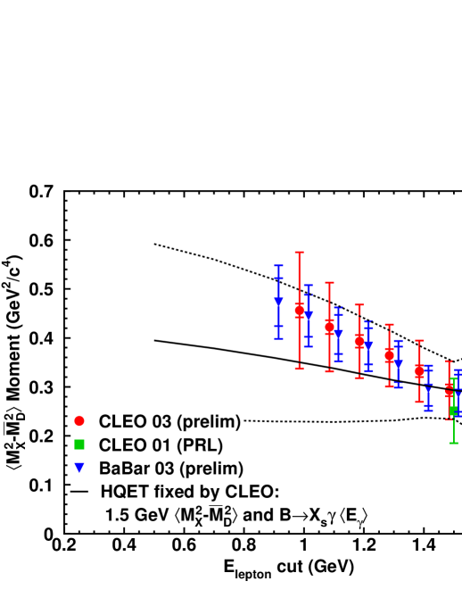
Figure 3: Comparison of BABAR ’03 [85], CLEO ’03 [92] and CLEO ’01  [87] measurements of the hadron invariant mass moment $\langle M_{X}^{2}-\bar{M}_{D}^{2}\rangle$ vs.lepton energy cut. The bands show the parametric uncertainties from theory [79]. (Figure taken from the CLEO paper [92] .)

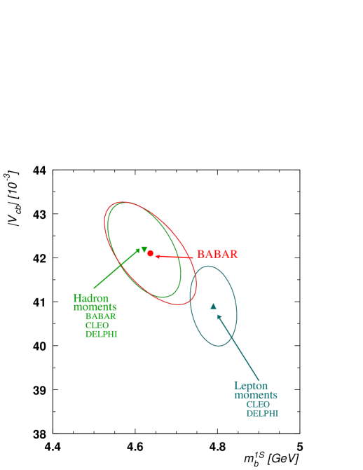
Figure 4: Constraints on the HQET parameters obtained from hadronic moments as measured by BABAR [85], hadronic moments combined (BABAR [85], CLEO [88], and  DELPHI [93]) and the combined lepton energy moments (CLEO [84] and DELPHI [93]) in the $(|V_{cb}|,m_{b}^{1S})$ plane. (Figure taken from the BABAR paper [85] .)

4.3 Determination of $|V_{cb}|$ from exclusive decays $B\rightarrow(D,D^{*})\ell\nu_{\ell}$

In exclusive decays, $B\rightarrow(D,D^{*})\ell\nu_{\ell}$, one needs to know the hadronic matrix elements of the charged weak current, $\langle D|J_{\mu}|B\rangle$ and $\langle D^{*}|J_{\mu}|B\rangle$. The former involves two form factors, called $F_{+}(q^{2})$ and $F_{0}(q^{2})$, and for the transition to the $D^{*}$-meson, one has four such form factors, called in the literature by the symbols $V(q^{2})$, $A_{i}(q^{2})$, $i=1,2,3$. If these form factors can be measured over a large-enough range of $q^{2}$ and the same can be obtained from a first principle calculation, such as lattice QCD, then exclusive decays would provide the best determination of $|V_{cb}|$. In the absence of a first principle calculation of these form factors, HQET provides a big help in that the heavy quark symmetries in HQET allow to reduce the number of independent form factors from six in the decays at hand to just one, called the Isgur-Wise (IW) function [94] ${\cal F}(\omega)$, where $\omega=v.v^{\prime}$, with $v$ and $v^{\prime}$ being the four-velocities of the $B$ and $D(D^{*})$ meson, respectively. Moreover, HQET provides a normalization of the IW function at the symmetry point, $\omega=1$. A lot of attention has been paid to the decay $B\rightarrow D^{*}\ell\nu_{\ell}$ due to Luke’s theorem [95], which states that symmetry-breaking corrections to ${\cal F}(\omega=1)$ are of second order, a situation very much akin to the Ademollo-Gatto theorem for the $K_{\ell 3}$ form factor $f_{+}(0)$ discussed earlier.

The differential decay rate for $B\rightarrow D^{*}\ell\nu_{\ell}$ can be written as

$$\frac{d\Gamma}{d\omega}=\frac{G_{F}^{2}}{4\pi^{3}}\left(\omega^{2}-1\right)^{1/2}\,m_{D^{*}}^{3}\,(m_{B}-m_{D^{*}})^{2}\,{\cal G}(\omega)\,|V_{cb}|^{2}\,|{\cal F}(\omega)|^{2}\,,$$ (59)

where ${\cal G}(\omega)$ is a phase space factor with ${\cal G}(1)=1$. Theoretical issues are then confined to a precise determination of the second order corrections to ${\cal F}(\omega=1)$, the slope of this function, $\rho^{2}$, and its curvature $c$,

$${\cal F}(\omega)={\cal F}(1)\,\left[1+\rho^{2}(\omega-1)+c(\omega-1)^{2}+...\right]\,.$$ (60)

In terms of the perturbative (QED and QCD) and the non-perturbative (leading $\delta_{1/m^{2}}$ and subleading $\delta_{1/m^{3}}$) corrections, the normalization of the Isgur-Wise function ${\cal F}(1)$ can be expressed as follows:

$${\cal F}(1)=\eta\,\left[1+\delta_{1/m^{2}}+\delta_{1/m^{3}}\right]\,,$$ (61)

where $\eta$ is the perturbative renormalization of the Isgur-Wise function, known to two loops, $\eta=0.960\pm 0.007$ [96, 97]. The formalism for calculating $\delta_{1/m^{2}}$ corrections in HQET has been developed by Falk and Neubert [98] and Mannel [99]. The various non-perturbative parameters entering in $\delta_{1/m^{2}}$ and the slope $\rho^{2}$ have been studied in the context of quark models [100], sum rules [101, 102, 103, 104, 105] and quenched Lattice QCD [106, 107]. The default value used in the BABAR Physics Book [108], ${\cal F}(1)=0.91\pm 0.04$, has recently been confirmed in the quenched lattice QCD calculations, including also $\delta_{1/m^{3}}$ corrections [106]. The slope $\rho^{2}$ is obtained by a simultaneous fit of the data for ${\cal F}(1)|V_{cb}|$ and $\rho^{2}$, and experiments use a form for ${\cal F}(\omega)$ given by Caprini et al. [109]. The resulting values of ${\cal F}(1)|V_{cb}|$ and the ${\cal F}(1)|V_{cb}|$ - $\rho^{2}$ correlation from a large number of measurements from the LEP experiments, CLEO, BELLE and BABAR are summarized in Fig. 5. They lead to the following world averages [59]:

$${\cal F}(1)|V_{cb}|=(36.7\pm 0.8)\times 10^{-3}\,,\qquad\rho^{2}=1.44\pm 0.14\,\,\,\,\,[\chi^{2}=30.3/14]\,,$$ (62)

which with the value ${\cal F}(1)=0.91\pm 0.04$ leads to

$$|V_{cb}|_{B\rightarrow D^{*}\ell\nu_{\ell}}=(40.2\pm 0.9_{\rm exp}\pm 1.8_{\rm theo})\times 10^{-3}\,.$$ (63)

This value is in very good accord with the determinations of $|V_{cb}|$ from the inclusive decays $B\rightarrow X_{c}\ell\nu_{\ell}$ given in (56) for the $\Upsilon(1S)$-scheme. While this consistency is striking, the agreement among the various experiments in the ${\cal F}(1)|V_{cb}|$ - $\rho^{2}$ correlation from the decay $B\rightarrow D^{*}\ell\nu_{\ell}$ is less so, having a rather high $\chi^{2}$, $\chi^{2}/d.o.f.=2.16$. A robust average for $|V_{cb}|$ from both the inclusive and exclusive decays is not yet available from the Heavy Flavor Averaging Group HFAG [59]. It is also not clear to me how to do this as $|V_{cb}|$ from the inclusive measurements is obtained in the $\Upsilon(1S)$ scheme, as the quark masses have been defined in this scheme in the analysis of data, whereas $|V_{cb}|$ from the exclusive decays does not have this dependence. An average can be given by weighting the two measurements with their experimental errors only, leaving the theoretical errors as they are, or one could add them in quadrature assuming they are independent. This gives

$$|V_{cb}|=(41.2\pm 0.8_{\rm exp}\pm 2.0_{\rm theo})\times 10^{-3}=(41.2\pm 2.1)\times 10^{-3}\,,$$ (64)

yielding a precision $\delta|V_{cb}|/|V_{cb}|\simeq 5\%$. In view of the still open issues (such as duality-related error, quark mass scheme-dependence in the inclusive decay, large $\chi^{2}/{\rm d.o.f.}$ in $B\rightarrow D^{*}\ell\nu_{\ell}$ decay, which makes the various experiments compatible with each other only at the expense of an increased error, etc.), a more precise value of $|V_{cb}|$, in my opinion, is not admissible at present. However, despite all the caveats, the achieved precision in $|V_{cb}|$ is indeed remarkable.

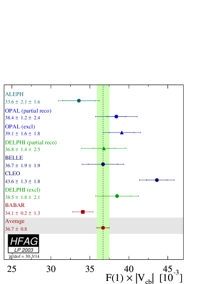
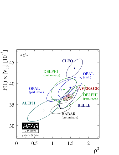
Figure 5: Present status of $F(1)|V_{cb}|$ (left frame) and the $F(1)|V_{cb}|$ - $\rho^{2}$ correlation (right frame) from $B\rightarrow D^{*}\ell\nu_{\ell}$ decays. Note that $F(1)$ is called ${\cal F}(1)$ in the text. (Figures taken from the Heavy Flavor Averaging Group [HFAG LP2003] [59] .)

4.4 Present status of $|V_{ub}|$

Essentially, there are two methods to measure $|V_{ub}|$. The first one analyses the inclusive decays $B\rightarrow X_{u}\ell\nu_{\ell}$, for which the branching ratio lies about a factor 60 below the dominant process $B\rightarrow X_{c}\ell\nu_{\ell}$. This circumstance makes it mandatory to apply harsh cuts to tag well the $b\rightarrow u$ events, invariably bringing in its wake theoretical problems involving enhanced non-perturbative and perturbative effects. The second method involves the exclusive decays, such as $B\rightarrow(\pi,\rho,\omega)\ell\nu_{\ell}$, which require good knowledge of the form factors, not yet completely under theoretical control. We briefly summarize the present status for both the inclusive and exclusive determinations of $|V_{ub}|$.

4.5 $|V_{ub}|$ from inclusive measurements

The theoretical framework to study the inclusive decays $B\rightarrow X_{u}\ell\nu_{\ell}$ is also based on the operator product expansion. Up to $O(1/m_{b}^{2})$ order, the result for $\Gamma(B\rightarrow X_{u}\ell\nu_{\ell})$ can be expressed as follows [110]:

$$\Gamma(B\rightarrow X_{u}\ell\nu_{\ell})=\frac{G_{F}^{2}m_{b}^{5}|V_{ub}|^{2}}{192\pi^{3}}\,\left(1-2.41\,\frac{\alpha_{s}(m_{b})}{\pi}-21.3\,\left(\frac{\alpha_{s}}{\pi}\right)^{2}+\frac{\lambda_{1}-9\lambda_{2}}{2m_{b}^{2}}+...\right)\,,$$ (65)

of which the first three terms are coming from the perturbative-QCD improved parton decay $b\rightarrow u\ell\nu_{\ell}$. The largest uncertainty in the decay rate is due to the $b$-quark mass, $m_{b}$, which is also scheme dependent, as already discussed. In the $\Upsilon(1S)$-scheme, the result for $|V_{ub}|$ is numerically expressed as follows [77]:

$$|V_{ub}|=(3.04\pm 0.06_{(\rm pert)}\pm 0.08_{(m_{b})})\times 10^{-3}\,\bigg{(}{{\cal B}(B\rightarrow X_{u}\ell\bar{\nu})\over 0.001}{1.6\,{\rm ps}\over\tau_{B}}\bigg{)}^{1/2}\,,$$ (66)

where the first error has a perturbative origin and the second is from $\Delta m_{b}$ in the $\Upsilon(1S)$-scheme, $m_{b}^{1S}=(4.73\pm 0.05)$ GeV. If this rate can be measured without significant cuts, then $|V_{ub}|$ can be measured with an accuracy of $O(5\%)$. We shall take this as an ideal case and discuss now the realistic cases when kinematic cuts are imposed on some of the variables to measure the $b\rightarrow u$ semileptonic decays.

As already mentioned, the dominant background is from the decays $B\rightarrow X_{c}\ell\nu_{\ell}$. Noting that the lowest mass hadronic state in $B\rightarrow X_{c}\ell\nu_{\ell}$ is the $D$-meson, thus its mass $m_{D}$ is used to define the cut region to suppress $b\rightarrow c$ transitions. So, the kinematic cut is either (i) on the upper end of the lepton energy spectrum, with $E_{\ell}>(m_{B}^{2}-m_{D}^{2})/2m_{B}$, or (ii) on the momentum transfer squared of the $\ell\nu_{\ell}$ pair, $q^{2}>(m_{B}-m_{D})^{2}$, or (iii) on the hadron invariant mass, $m_{X}<m_{D}$, or (iv) an optimized combination of some or all of them. These cuts reduce the experimental rates for $B\rightarrow X_{u}\ell\nu_{\ell}$, a handicap which will be overcome at B-factories with $O(10^{8})$ $B\bar{B}$ mesons already at hand. However, the cuts also make the theoretical rates less rapidly convergent in terms of the perturbation series in $\Lambda_{\rm QCD}/m_{b}$ and $\alpha_{s}(m_{b})$. The other disadvantage is that the theoretical rate with a cut depends sensitively (except for a cut on $q^{2}$) on the details of the $B$-meson wave function, or the shape function $f(k_{+})$ [111]. Here $k_{+}$ is the $+$ component (using light cone variables) of a residual momentum $k_{\mu}$ of order $\Lambda_{\rm QCD}$, entering through the relation $p_{b}^{\mu}=m_{b}v^{\mu}+k^{\mu}$, where $p_{b}^{\mu}$ is the momentum of the $b$-quark in the $B$ meson, and $v^{\mu}$ is the four-velocity of the quark. This can be seen as follows. With either of the two cuts, $E_{\ell}>(m_{B}^{2}-m_{D}^{2})/2m_{B}$, or for the small hadronic invariant mass region, $m_{X}<m_{D}$, we have

$$E_{X}\sim m_{b}\,;\quad m_{X}^{2}=(m_{b}v-q)^{2}+2E_{X}k_{+}+...,$$ (67)

bringing in the dependence on $k_{+}$. This dependence is rather mild using the cuts on $q^{2}$. The effects of the kinematic cuts on the decay distributions and rates have been studied at great length in the literature. In fact, this enterprise has led to a flourishing industry - the (kinematic) cutting technology using HQET [112, 113, 114, 115, 116, 117, 118, 119, 120, 121]! Some applications are discussed here.

In the leading order in $\Lambda_{\rm QCD}/m_{b}$, there is a universal function which governs the shape of the charged lepton energy spectrum, the hadronic invariant mass spectrum in $B\rightarrow X_{u}\ell\nu_{\ell}$ and the photon energy spectrum in $B\rightarrow X_{s}\gamma$, defined as follows [122]

$$f(k_{+})=\frac{1}{2m_{B}}\langle B(v)|\bar{b}_{v}\delta(k_{+}+iD.n)b_{v}|B(v)\rangle\,,$$ (68)

where $n$ is a light-like vector satisfying $n.v=1$ and $n^{2}=0$. The physical spectra are obtained by convoluting the universal shape function with the perturbative-QCD expressions. Ignoring the perturbative and subleading power corrections, a measurement of the photon energy spectrum is a measurement of the shape function $f(k_{+})$:

$$\frac{m_{b}}{2\Gamma^{(0)}_{\rm sl}}\,\frac{d\Gamma}{dE_{l}}(B\rightarrow X_{u}l\nu_{l}) = \int d\omega\,\theta\left(m_{b}-2E_{l}-\omega\right)\,f(\omega)+\ldots,$$ (69)

$$\frac{1}{\Gamma^{(0)}_{\gamma}}\,\frac{d\Gamma}{dE_{\gamma}}(B\rightarrow X_{s}\gamma) = \int d\omega\,\delta\left(m_{b}-2E_{\gamma}-\omega\right)\,f(\omega)+\ldots=f(m_{b}-2E_{\gamma})+\ldots,$$

where the normalization constants for the semileptonic and radiative $B$-meson decays are:

$$\Gamma^{(0)}_{\rm sl} = \frac{G_{F}^{2}|V_{ub}|^{2}m_{b}^{5}}{192\pi^{3}}\equiv C_{\rm sl}\,|V_{ub}|^{2},$$

$$\Gamma^{(0)}_{\gamma} = \frac{G_{F}^{2}\alpha|V_{tb}V_{ts}^{*}|^{2}m_{b}^{5}}{32\pi^{4}}\,\,|C_{7}^{\rm eff}|^{2}\equiv C_{\gamma}\,|V_{tb}V_{ts}^{*}|^{2},$$ (70)

and $C_{7}^{\rm eff}$ is the effective Wilson coefficient governing the decay $B\rightarrow X_{s}\gamma$. Thus, combining the data on $B\rightarrow X_{s}\gamma$ and the lepton energy spectrum from $B\rightarrow X_{u}\ell\nu_{\ell}$, one can determine in the SM the following ratio:

$$\left|\frac{V_{ub}}{V_{tb}V_{ts}^{*}}\right|^{2}=3\,\frac{\alpha}{\pi}\,\left|C_{7}^{\rm eff}\right|^{2}\frac{\Gamma_{u}(E_{c})}{\Gamma_{s}(E_{c})}+O\left(\alpha_{s}\right)+O\left(\frac{\Lambda_{\rm QCD}}{m_{b}}\right)\,,$$ (71)

where $\Gamma_{u}(E_{c})$ and $\Gamma_{s}(E_{c})$ are the cut-off dependent decay width in $\Gamma(B\rightarrow X_{u}\ell\nu_{\ell};~{}E_{\ell}>E_{c})$ and the cut-off dependent first moment of the photon energy spectrum, respectively

$$\Gamma_{u}(E_{c}) \equiv \int_{E_{c}}^{m_{B}/2}dE_{\ell}\,\frac{d\Gamma_{u}}{dE_{\ell}}\,,$$

$$\Gamma_{s}(E_{c}) \equiv \frac{2}{m_{b}}\int_{E_{c}}^{m_{B}/2}dE_{\gamma}\left(E_{\gamma}-E_{c}\right)\frac{d\Gamma_{s}}{dE_{\gamma}}\,.$$ (72)

It should be stressed that the ratio (71) holds not only in the SM, but also in models where the flavour changing (FC) transition $b\rightarrow s$ is enacted solely in terms of $V_{\rm CKM}$, such as the minimal flavour violating supersymmetric models. An example where this relation does not hold is a general supersymmetric model in which the couplings $d_{i}\tilde{s}_{j}\tilde{g}$, involving a down-type quark, a squark and gluino, are not diagonal in the flavour $(ij)$ space. In that case, the decay width for $B\rightarrow X_{s}\gamma$ does not factorize in $|V_{tb}V_{ts}^{*}|^{2}$ and depends on additional FC parameters.

The relation (71) has been put to good use, in the context of the SM, by the CLEO collaboration [123] through the measurement of the photon-energy spectrum in $B\rightarrow X_{s}\gamma$ [89] and the lepton energy spectrum in $B\rightarrow X_{u}\ell\nu_{\ell}$, with 2.2 GeV $<E_{\ell}<2.6$ GeV, as the photon energy spectrum has been well measured in the overlapping range for $E_{\gamma}$, yielding

$$|V_{ub}|=(4.08\pm 0.34\pm 0.44\pm 0.16\pm 0.24)\times 10^{-3}\,,$$ (73)

where the first two uncertainties are of experimental origin and the last two are theoretical, of which $\delta|V_{ub}|=\pm 0.24\times 10^{-3}$ is an assumed uncertainty in the relation (71). Combining all the errors in quadrature leads to $|V_{ub}|=(4.08\pm 0.63)\times 10^{-3}$, which is a $\pm 15\%$ measurement of this matrix element.

This method of determining $|V_{ub}|$ pioneered by the CLEO collaboration has received a lot of theoretical attention lately. In particular, the subleading-twist contributions to the lepton and photon energy spectra in the decays $B\rightarrow X_{u}\ell\nu_{\ell}$ and $B\rightarrow X_{s}\gamma$, respectively, have been calculated in a number of papers [124, 125, 126, 127], providing estimates of the subleading correction in (71) indicated as $O(\frac{\Lambda_{\rm QCD}}{m_{b}})$. An important feature emerging from these studies is that the various spectra are no longer governed by a universal shape function $f(\omega)$, a feature which is valid only in the leading twist. In subleading twist, HQET shows its rich underlying structure leading to a number of additional subleading shape functions, which are no longer universal. The operators ${\cal O}_{i}$ needed to calculate the subleading twist contributions and the corresponding matrix elements (shape functions) of these operators $\langle B|{\cal O}_{i}|B\rangle$ can be found, for example, in the papers by Bauer, Luke and Mannel [124, 125]. The photon energy spectrum in $B\rightarrow X_{s}\gamma$ can now be expressed in terms of three structure functions $F(\omega)$, $h_{1}(\omega)$ and $H_{2}(\omega)$ as follows [124]

$$\frac{m_{b}}{C_{\gamma}}\frac{d\Gamma}{dE_{\gamma}}=\left|V_{tb}V_{ts}^{*}\right|^{2}\left[(4E_{\gamma}-m_{b})F(m_{b}-2E_{\gamma})+\frac{1}{m_{b}}\bigg{(}h_{1}(m_{b}-2E_{\gamma})+H_{2}(m_{b}-2E_{\gamma})\bigg{)}+{\cal O}\left(\frac{\Lambda_{\rm QCD}^{2}}{m_{b}^{2}}\right)\right],$$

(74)

where $C_{\gamma}$ has been defined earlier. Here, $F(\omega)$ contains both the leading and sub-leading parts with $F(\omega)=f(\omega)+{\cal O}(\Lambda_{\rm QCD}/m_{b})$, and $h_{1}(\omega)$ and $H_{2}(\omega)$ are the subleading shape functions.

The corresponding lepton energy spectrum in the decay $B\rightarrow X_{u}\ell\nu_{\ell}$ now has the following form [125]:

$$\frac{m_{b}}{2C_{\rm sl}}\frac{d\Gamma}{dE_{\ell}}=|V_{ub}|^{2}\left[\int d\omega\,\theta\,(m_{b}-2E_{\ell}-\omega)\left(F(\omega)\left(1-\frac{\omega}{m_{b}}\right)-\frac{1}{m_{b}}h_{1}(\omega)+\frac{3}{m_{b}}H_{2}(\omega)\right)+{\cal O}\left(\frac{\Lambda_{\rm QCD}^{2}}{m_{b}^{2}}\right)\right],$$

where $C_{\rm sl}$ has also been defined earlier. It is obvious that the measurement of either the photon energy spectrum or the lepton energy spectrum does not allow to determine all three shape functions. Hence, they will have to be modeled. These subleading corrections modify the relation (71) used in extracting $|V_{ub}|$, which can be written as[125]:

$$\left|\frac{V_{ub}}{V_{tb}V_{ts}^{*}}\right|=\bigg{(}3\,\frac{\alpha}{\pi}\,|C_{7}^{\rm eff}|^{2}\,\frac{\Gamma_{u}(E_{c})}{\Gamma_{s}(E_{c})}\bigg{)}^{1/2}\left(1+\delta(E_{c})\right)\,.$$ (76)

Again, $\delta(E_{c})$ can only be estimated in a model-dependent way. Typical estimates are $\delta(E_{c}=2.2~{}{\rm GeV})\simeq 0.15$, with $\delta(E_{c})$ decreasing as the lepton-energy cut $E_{c}$ decreases, estimated as $O(10\%)$ for $E_{c}=2.0~{}{\rm GeV}$. One should use the order of magnitude estimate of the subleading twist contribution $\delta(E_{c})$ to set the theoretical uncertainty on $|V_{ub}|$ from this method, which typically is $15\%$.

These uncertainties can be reduced if one considers more complicated kinematic cuts, such as a simultaneous cut on $m_{X}$ and $q^{2}$ [119, 55], whose effect has been studied using a model for the leading-twist shape function $f(k_{+})$. The sensitivity of the partial decay width $\Gamma(q^{2}>q^{2}_{\rm cut},m_{X}<m_{\rm cut})$ on $f(k_{+})$ is found to be small, and this is likely to hold also if the subleading shape functions are included. This method of determining $|V_{ub}|$ has been applied by BELLE using two techniques. The first uses the decays $B\rightarrow D^{(*)}\ell\nu_{\ell}$ as a tag, and the other uses the neutrino reconstruction technique, as in exclusive semileptonic decays, combined with a sorting algorithm (called ”annealing”) to separate the event in a tag and a $b\rightarrow u\ell\nu_{\ell}$ side. The method based on $D^{(*)}$-tagging yields[128] $|V_{ub}|=(5.0\pm 0.64\pm 0.53)\times 10^{-3}$. The result using the annealing method with the cuts $m_{X}<1.7$ GeV, $q^{2}>8$ GeV² is [129]

$$|V_{ub}|=(4.66\pm 0.28\pm 0.35\pm 0.17\pm 0.08\pm 0.58)\times 10^{-3}\,,$$ (77)

where the errors are statistical, detector systematics, modeling $b\rightarrow c$, modeling $b\rightarrow u$, and theoretical, respectively. Combining all the errors yields $|V_{ub}|=(4.66\pm 0.76)\times 10^{-3}$.

A similar analysis by the BABAR collaboration, in which one of the two $B$-mesons is constructed through the hadronic decays $B\rightarrow D^{(*)}h$, and the inclusive semileptonic decay of the other $\bar{B}$-meson is measured with the cuts $E_{\ell}>1$ GeV and $m_{X}<1.55$ GeV [130], yields

$$|V_{ub}|=(4.52\pm 0.31\pm 0.27\pm 0.40\pm 0.25)\times 10^{-3}\,,$$ (78)

where the errors are statistical, systematics, due to extrapolations to the full phase space, and from the HQET parameters, respectively.

Finally, the effects of the so-called weak annihilation (WA) [131], which are formally of $O(\Lambda_{\rm QCD}^{3}/m_{b}^{3})$ but are enhanced by the phase space factor $16\pi^{2}$ (compared to that of $b\rightarrow u\ell\nu_{\ell}$), introduce an additional theoretical uncertainty [132]. They stem from the dimension-6 four-quark operators in the OPE,

$$O_{V-A}=(\bar{b}_{v}\gamma_{\mu}P_{L}u)(\bar{u}\gamma^{\mu}P_{L}b_{v})\,,\qquad O_{S-P}=(\bar{b}_{v}P_{L}u)(\bar{u}P_{R}b_{v})\,,$$ (79)

where $P_{L,R}=(1\pm\gamma_{5})/2$. In the lepton energy spectrum from $B\rightarrow X_{u}\ell\nu_{\ell}$, they enter as delta functions near the end-point [132]:

$$\frac{d\Gamma_{(6)}}{dy}=-\frac{G_{F}^{2}m_{b}^{2}|V_{ub}|^{2}}{12\pi}\,f_{B}^{2}\,m_{B}\,(B_{1}-B_{2})\,\delta(1-y)\,,$$ (80)

where $y=2E_{\ell}/m_{b}$ and $f_{B}\simeq 200$ MeV is the $B$ meson decay constant; $B_{1}$ and $B_{2}$ parameterize the matrix elements of the operators $O_{V-A}$ and $O_{S-P}$, respectively:

$$\frac{1}{2m_{B}}\langle B|O_{V-A}|B\rangle=\frac{f_{B}^{2}m_{B}}{8}\,B_{1}\,,\qquad\frac{1}{2m_{B}}\langle B|O_{S-P}|B\rangle=\frac{f_{B}^{2}m_{B}}{8}\,B_{2}\,.$$ (81)

In the vacuum insertion approximation, i.e., assuming factorization, their effect in the spectrum vanishes, as in this approximation, $B_{1}=B_{2}=1(0)$ for the charged (neutral) $B$ mesons. Hence, they are generated by non-factorizing contributions and are not yet quantified. These matrix elements are also encountered in calculating the differences in the $B^{\pm}$ and $B^{0}$ lifetimes [133], and we refer to a recent discussion in the context of lattice QCD [134]. However, comparing the extraction of $|V_{ub}|$ from $B^{\pm}\rightarrow X_{u}\ell\nu_{\ell}$ and $B^{0}\rightarrow X_{u}\ell\nu_{\ell}$ near the end-point of the lepton energy spectrum, one can determine the size of the WA effects. For the $B^{\pm}$ decays, they can also be estimated from a related process $B^{\pm}\rightarrow\ell^{\pm}\nu_{\ell}\gamma$ [135].

The current results on $|V_{ub}|$ from various inclusive measurements by the LEP, CLEO, BABAR and BELLE experiments are summarized by HFAG [59]. No averaging for $|V_{ub}|$ has been undertaken so far by this working group. However, the results in (73), (77) and (78) from the CLEO, BELLE and BABAR collaborations, respectively, have been averaged by Muheim [136] to get $|V_{ub}|$ from the $\Upsilon(4S)$ data, yielding

$$|V_{ub}|_{\rm incl}=(4.32\pm 0.57)\times 10^{-3}\,,$$ (82)

in agreement with the LEP average [137] $|V_{ub}|=(4.09\pm 0.70)\times 10^{-3}$.

4.6 $|V_{ub}|$ from exclusive measurements

First measurements of the exclusive decays $B\rightarrow\pi\ell\nu_{\ell}$ and $B\rightarrow\rho\ell\nu_{\ell}$ were reported by the CLEO collaboration in 1996 [138]. Improved measurements of the rates for $B\rightarrow\rho\ell\nu_{\ell}$ were published subsequently [139]. This year, results based on the entire CLEO data ($9.7\times 10^{6}~{}B\overline{B}$ pairs) were reported  [140], including the measurement of the branching ratio for $B^{+}\rightarrow\eta\ell^{+}\nu_{\ell}$ (charge conjugation average is implied):

$${\cal B}(B^{0}\rightarrow\pi^{-}\ell^{+}\nu_{\ell}) = (1.33\pm 0.18\pm 0.11\pm 0.01\pm 0.07)\times 10^{-4}\,,$$

$${\cal B}(B^{0}\rightarrow\rho^{-}\ell^{+}\nu_{\ell}) = (2.17\pm 0.34^{+0.47}_{-0.54}\pm 0.41\pm 0.01)\times 10^{-4}\,,$$ (83)

$${\cal B}(B^{+}\rightarrow\eta\ell^{+}\nu_{\ell}) = (0.84\pm 0.31\pm 0.16\pm 0.09)\times 10^{-4}\,,$$

where the errors are statistical, experimental systematic, form factor uncertainties in the signal, and form factor uncertainties in the cross-feed modes, respectively. Rough measurement of the $q^{2}$ distributions $d\Gamma(q^{2})/dq^{2}$ for the $(\pi\ell\nu_{\ell})$ and $(\rho\ell\nu_{\ell})$ modes by splitting the data in three $q^{2}$-bins were also reported. BABAR has also measured the decay $B\rightarrow\rho\ell\nu_{\ell}$ [141]:

$${\cal B}(B^{0}\rightarrow\rho^{-}\ell^{+}\nu_{\ell})=(3.29\pm 0.42\pm 0.47\pm 0.60)\times 10^{-4}\,,$$ (84)

where the errors are statistical, systematic and theoretical, respectively.

Extracting $|V_{ub}|$ from these measurements is done by using quark models, QCD sum rules, and quenched Lattice-QCD calculations for the form factors. We discuss the two main contenders, Lattice QCD and QCD sum rules, for the semileptonic decays $B\rightarrow\pi\ell\nu_{\ell}$, as this involves (neglecting the lepton mass) only one form factor, $F_{+}(q^{2})$, defined as follows:

$$\langle\pi(p_{\pi})|\bar{b}\gamma_{\mu}q|B(p_{B})\rangle=\left((p_{B}+p_{\pi})_{\mu}-\frac{m_{B}^{2}-m_{\pi}^{2}}{q^{2}}q_{\mu}\right)\,F_{+}(q^{2})+\frac{m_{B}^{2}-m_{\pi}^{2}}{q^{2}}\,F_{0}(q^{2})\,q_{\mu}\,,$$ (85)

with $F_{+}(0)=F_{0}(0)$.

QCD sum rules [142], in particular Light cone QCD sum rules (LCSRs) [143, 144], have been used extensively to study the form factors in $B\rightarrow\pi$ transitions (and other related processes) [62]. In the LCSR, one calculates a correlation function involving the weak current and an interpolating current with the quantum numbers of the $B$ meson, sandwiched between the vacuum ($\langle 0|$) and a pion state ($|\pi\rangle)$:

$$F_{\mu}(p,q)=i\int dx{\rm e}^{iq.x}\langle\pi(p)|T\{\bar{u}(x)\gamma_{\mu}b(x),m_{b}\bar{b}(0)i\gamma_{5}d(0)\}|0\rangle\,.$$ (86)

For large negative virtualities $(q^{2},p.q)$ of these currents, the correlation function (CF) in the coordinate space is dominated by the dynamics at distances near the light cone, allowing a light-cone expansion of the CF (hence, the name). In essence, LCSRs are based on the factorization property of the CF into non-perturbative light-cone distribution amplitudes (LCDAs) of the pion, called $\phi_{\pi}^{n}(u,\mu)$, where $u$ is the fractional momentum of the quark in the pion and $\mu$ is a factorization scale, and process-dependent hard (perturbative QCD) amplitudes $T_{H}^{n}(\mu,m_{b},u,q^{2})$, where $q^{2}$ is the virtuality of the weak current. Schematically, the coefficients in front of the Lorentz structures in the decomposition of the CF (86) can be written as:

$$C(\mu,q^{2},m_{b})\sim\sum_{n}T_{H}^{n}(\mu,m_{b},u,q^{2})\otimes\phi^{n}(u,\mu)\,,$$ (87)

where the sum runs over contributions with increasing twist, with twist-2 being the lowest, and the symbol $\otimes$ implies an integration over the variable $u$. The amplitudes $T_{H}^{n}$ have an expansion in perturbative QCD (i.e., $\alpha_{s}$). The same correlation function can also be written as a dispersion relation in the virtuality of the current coupled to the $B$-meson. Equating the two, using quark-hadron duality, and separating the $B$-meson contribution from higher excited and continuum states, results in the LCSR. As an illustration, the LCSR for the form factor $F_{+}(q^{2})$ in the lowest order in $\alpha_{s}$ and leading-twist has the form [62]

$$F_{+}(q^{2})=\frac{1}{2m_{B}^{2}f_{B}}{\rm e}^{~{}-\frac{m_{B}^{2}}{M^{2}}}m_{b}^{2}f_{\pi}\int_{\Delta}^{1}\frac{du}{u}{\rm e}^{-\frac{m_{b}^{2}-p^{2}(1-u)}{uM^{2}}}\phi_{\pi}(u,\mu_{b})\,,$$ (88)

where $f_{\pi}=132$ MeV, M is a Borel parameter, characterizing the off-shellness of the $b$-quark, and $\phi_{\pi}(u,\mu_{b})$ is the twist-2 LCDA of the pion

$$\phi_{\pi}(u,\mu)=6u(1-u)\left(1+a_{2}^{\pi}(\mu)C_{2}^{3/2}(2u-1)+...\right)\,.$$ (89)

Here, $C_{2}^{3/2}(x)$ is a Gegenbauer polynomial and $a_{2}^{\pi}(\mu)$ is a non-perturbative coefficient (the second Gegenbauer moment) to be determined, for example, from the data on the electromagnetic form factor of the pion. The lower integration limit denoted by $\Delta$ is defined through $\Delta=(m_{b}^{2}-q^{2})/(s_{0}^{B}-q^{2})$, where $s_{0}^{B}$ is determined by the subtraction point of the excited resonances and continuum states contributing to the dispersion integral in the $B$ channel. Assuming quark-hadron duality, this subtraction is performed at $(p+q)^{2}\geq s_{0}^{B}$.

In principle, given the assumption of quark-hadron duality, the LCSRs can be made arbitrarily accurate, by calculating enough perturbative and non-leading twist contributions to the CF. In practice, this framework has a number of parameters (such as $\mu$, $M$, $a_{i}^{\pi}(\mu)$, $s_{0}^{B}$, $m_{b}$), whose imprecise knowledge restricts the precision on the CF. Typically, the state-of-the-art LCSRs for $F_{+}(q^{2})$ [145, 146, 147], which include $\alpha_{s}$ corrections to the leading-twist and part of the twist-three contributions, and tree level for rest of the twist-three and twist-four, have an uncertainty of $\sim\pm 20\%$ [62, 148], and it is probably difficult to make these estimates more precise.

In Lattice QCD, one calculates a three-point correlation function involving interpolating operators for the $B$ and $\pi$ mesons and the vector current $V_{\mu}\sim\bar{\Psi}_{b}\gamma_{\mu}\Psi_{q}$. In the limit of a large time separation, the correlation function has the following behaviour

$$C_{\mu}(p,k,t_{f},t_{s},t_{i})={\cal Z}_{B}^{1/2}\,{\cal Z}_{\pi}^{1/2}\,\frac{\langle B(k)|V_{\mu}|\pi(p)\rangle}{\sqrt{2E_{B}}\,\,\sqrt{2E_{\pi}}}\,{\rm e}^{-E_{\pi}(t_{s}-t_{i})}\,{\rm e}^{-E_{B}(t_{f}-t_{s})}\,,$$ (90)

where $E_{B}(E_{\pi})$ is the energy of a $B(\pi)$ meson with the three-momentum $k(p)$ and ${\cal Z}_{B}^{1/2}({\cal Z}_{\pi}^{1/2})$ is the external line factor calculated from the two-point correlation functions involving the interpolating $B(\pi)$ fields. Since, one has to go to large time separations to suppress the continuum contribution, one is forced to restrict the pion momentum in $B\rightarrow\pi\ell\nu_{\ell}$ decay to low values. Hence, in lattice calculations, there is an upper limit on this momentum, $|p^{\rm max}|$, prescribed by the requirement to keep the statistical and discretization errors small. There is also a lower limit on $|p|$ dictated by the difficulty in extrapolations in $|p|$ and light quark masses. Thus, for example, the FNAL Lattice QCD calculations for the $B\rightarrow\pi$ form factors [149] have as cut-offs $|p^{\rm max}|=1.0$ GeV and $|p^{\rm min}|=0.4$ GeV. This translates into a limited $q^{2}$ range $q^{2}_{\rm min}<q^{2}<q^{2}_{\rm max}$ close to the zero-recoil point.

Recalling that the differential decay rate for $B\rightarrow\pi\ell\nu_{\ell}$ is given by

$$\frac{d\Gamma}{dp}(B\rightarrow\pi\ell\nu_{\ell})=\frac{G_{F}^{2}|V_{ub}|^{2}}{24\pi^{3}}\,\frac{2m_{B}p^{4}|F_{+}(E)|^{2}}{E}\,,$$ (91)

where $E=p_{\pi}.p_{B}/m_{B}$ is the pion energy in the $B$-meson rest frame, one calculates the dynamical part on the lattice over a limited region of $|p|$ [149]. Defining

$$T_{B}(|p^{\rm min}|,|p^{\rm max}|)\equiv\int_{|p^{\rm min}|}^{|p^{\rm max}|}dp\,\frac{p^{4}|F_{+}(E)|^{2}}{E}\,,$$ (92)

one combines the theoretical rate with the experimental measurements in the same momentum range of the pion to arrive at the following relation for $|V_{ub}|^{2}$,

$$|V_{ub}|^{2}=\frac{12\pi^{3}}{G_{F}^{2}m_{B}}\,\frac{1}{T_{B}(|p^{\rm min}|,|p^{\rm max}|)}\,\int_{|p^{\rm min}|}^{|p^{\rm max}|}dp\,\frac{d\Gamma(B\rightarrow\pi\ell\nu_{\ell})}{dp}\,.$$ (93)

This avoids the need to extrapolate to higher pion momenta (or low $q^{2}$). The practical problem in using (93) is the paucity of experimental data in low $|p|$-region, as the differential decay rate has a kinematic suppression for low pion momenta.

Alternatively, one has to use models for $q^{2}$ extrapolation of the Lattice results to lower values of $q^{2}$. This is done, for example, by the UKQCD [150] and the APE collaborations [45], which make use of the LCSRs (discussed above) to constrain the form factors at lower values of $q^{2}$.

Apart from this, there are also other systematic differences among the various Lattice calculations of the $B\rightarrow\pi$ form factors, the most important of which is related to the fact that for the current lattice spacing $a$ one has $m_{b}a>1$. To control lattice spacing effects, one has to do the calculations for values of the heavy quark mass $m_{Q}$ much smaller than $m_{b}$ and then extrapolate from $m_{Q}\simeq 1-2$ GeV, where the lattice data is available, to the $b$-quark mass. This, for example, is done by the UKQCD [150] and APE [45] collaborations. A different route is taken by the FNAL Lattice group [149], in which HQET is applied directly to the Lattice observables, using the same Wilson action for fermions as adopted by the other groups, but adjusting the couplings in the action and the normalization of the currents, so that the leading and the next-to-leading terms in HQET are correct. This allows to perform the calculations directly at $m_{Q}=m_{b}$. However, there are still some open issues in this approach what concerns the non-perturbative matching of the lattice with the continuum. Finally, JLQCD [151] also uses the Fermilab NRQCD approach. The result of the four Lattice groups for the $B\rightarrow\pi$ form factors, $F_{+}(q^{2})$ and $F_{0}(q^{2})$, are shown in Fig. 6, taken from the review by Becirevic [152]. These calculations agree at the level of $\pm 20\%$, though this consistency is less marked for the form factor $F_{0}(q^{2})$.

The results of the Lattice groups (APE [45], UKQCD [150], FNAL [149], and JLQCD [151]) have also been fitted by a phenomenological form for $F_{+,0}(q^{2})$ due to Becirevic and Kaidalov [153]

$$F_{+}(q^{2})=\frac{F(0)}{(1-q^{2}/m_{B^{*}}^{2})(1-\alpha_{\pi}q^{2}/m_{B^{*}}^{2})}\,;\qquad F_{0}(q^{2})=\frac{F(0)}{1-q^{2}/(\beta_{\pi}m_{B^{*}}^{2})},$$ (94)

involving three parameters $F(0)$, $\alpha_{\pi}$ and $\beta_{\pi}$. The best-fit solution for $F_{+}(q^{2})$ and $F_{0}(q^{2})$ is shown by the dashed curve in Fig. 6. This figure also shows the prediction obtained by the LCSRs [62]. The resulting theoretical description for the form factors from lattice QCD and LCSRs is strikingly consistent, albeit not better than $\pm 20\%$. Further details can be seen elsewhere [152].

In future, with more CPU power at their disposal, it should be possible to increase the pion momentum range accessible on the lattice, allowing a larger and statistically improved overlap of the lattice results with the experimental data on $B\rightarrow\pi\ell\nu_{\ell}$. Also, by using the FNAL method of applying HQET directly to the Lattice observables, or else by doing simulations at larger values of $m_{Q}$ than is the case right now, theoretical errors on the FFs can be reduced to an acceptable level in the quenched approximation. There are also other techniques being developed for treating heavy quarks on the Lattice [154]. The last step in this theoretical precision study will come with the estimates of unquenching effects using dynamical fermions; first unquenched results for $B\rightarrow\pi$ form factors are expected soon.

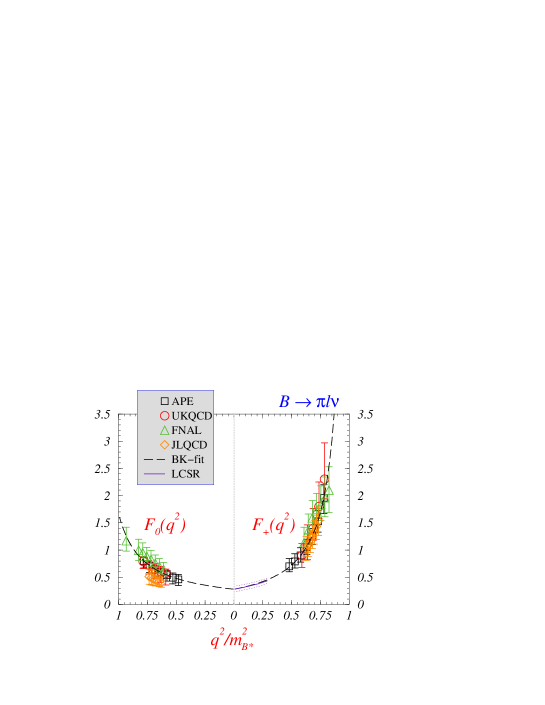
Figure 6: Summary of the current (unquenched) Lattice calculations of the $B\rightarrow\pi$ form factors $F_{0}(q^{2})$ and $F_{+}(q^{2})$ and from the Light Cone QCD sum rules. The dashed curve shows a parametrization by the Becirevic-Kaidalov model. (Figure taken from Becirevic [152] .)

After this longish detour of the currently used theoretical framework, we return to the extraction of $|V_{ub}|$ from exclusive semileptonic decays. The CLEO result [140] quoted below is obtained by using the quenched Lattice QCD results for $q^{2}>16$ GeV² and the LC QCD sum rules for lower values of $q^{2}$,

$$|V_{ub}|=(3.17\pm 0.17^{+0.16+0.53}_{-0.17-0.39}\pm 0.03)\times 10^{-3}~{}~{}[{\rm CLEO(exclusive)}]\,.$$ (95)

BABAR [141] uses the theoretical decay width calculated using Lattice QCD, LC QCD sum rules, and three quark models to estimate the form factors. The combined result is the weighted average of these theoretical approaches, where the weight is obtained by the theoretical uncertainty, and an overall theoretical uncertainty is assigned by taking it to be half of the full spread over these models. The result is [141]:

$$|V_{ub}|=(3.64\pm 0.22\pm 0.25^{+0.39}_{-0.56})\times 10^{-3}~{}~{}[{\rm BABAR}]\,.$$ (96)

The two measurements (95) and (96) are consistent with each other, and they have been averaged by Schubert [41] to yield a value of $|V_{ub}|$ from the exclusive decays,

$$|V_{ub}|_{\rm excl}=(3.40^{+0.24}_{-0.33}\pm 0.40)\times 10^{-3}\,.$$ (97)

However, this value lies below $|V_{ub}|$ measured from the inclusive decays $B\rightarrow X_{u}\ell\nu_{\ell}$, whose current average is given in (82). The mismatch in the values of $|V_{ub}|$ from the inclusive and exclusive decays is roughly about $20\%$ and has to be resolved as more precise data and theory become available. The possibility that in the quenched Lattice QCD and LCSR estimates, the form factor $F_{+}(q^{2})$ is estimated too high by about $20\%$ can not be excluded at present.

Digressing from the discussion of $|V_{ub}|$, we remark that this trend is also seen in the comparison of data on $B\rightarrow K^{*}\gamma$ with the LC-QCD sum rule estimates of the $B\rightarrow K^{*}$ form factors. To put this in a quantitative perspective, we recall that the current branching ratios for the $B\rightarrow K^{*}\gamma$ decays are [59] (again charge conjugated averages are implied)

$${\cal B}(B^{0}\rightarrow K^{*0}\gamma)=(4.17\pm 0.23)\times 10^{-5}\,,\qquad{\cal B}(B^{-}\rightarrow K^{*-}\gamma)=(4.18\pm 0.32)\times 10^{-5}\,.$$ (98)

The corresponding theoretical rates have been calculated in the NLO accuracy [155, 156, 157] using the QCD-factorization framework [158]. An updated analysis based on [155] (neglecting a small isospin violation in the decay widths) yields

$${\cal B}(B\rightarrow K^{*}\gamma)=(7.4\pm 1.0)\times 10^{-5}\left(\frac{\tau_{B}}{1.6~{}{\rm ps}}\right)\,\left(\frac{m_{b,{\rm pole}}}{4.65~{}{\rm GeV}}\right)^{2}\,\left(\frac{T_{1}^{K^{*}}(0,\bar{m}_{b})}{0.38}\right)^{2}\,,$$ (99)

where the default value for the form factor $T_{1}^{K*}(0,\bar{m}_{b})$ is taken from the LC-QCD sum rules [148] , and the pole mass $m_{b,~{}{\rm pole}}$ is the one-loop corrected central value obtained from the $\overline{\rm MS}$ $b$-quark mass $\bar{m}_{b}(m_{b})=(4.26\pm 0.15\pm 0.15)$ GeV in the PDG reviews [2]. Since the inclusive branching ratio for $B\rightarrow X_{s}\gamma$ in the SM agrees well with the current measurements of the same (discussed below), the mismatch in the estimates of the exclusive branching ratios in (99) and current measurements (98) in all likelihood has a QCD origin. Of the possible suspects, form factor is probably the most vulnerable link in the chain of arguments leading to (99). Interpreting the factorization-based QCD estimates and the data on their face value, good agreement between the two requires $T_{1}^{K^{*}}(0,\bar{m}_{b})\simeq 0.27\pm 0.02$. This is shown in Fig. 7 where the ratio

$$R(K^{*}\gamma/X_{s}\gamma)\equiv\frac{{\cal B}(B\rightarrow K^{*}\gamma)}{{\cal B}(B\rightarrow X_{s}\gamma)}\,,$$ (100)

is plotted as a function of $T_{1}^{K^{*}}(0,\bar{m}_{b})$. The horizontal bands show the current experimental value for this quantity $R(K^{*}\gamma/X_{s}\gamma)=0.125\pm 0.015$.

width=0.45file=RatKsT1.eps

Figure 7: The ratio of the branching ratios defined in Eq. (100), plotted as a function of the QCD form factor $T_{1}^{K^{*}}(0,\bar{m}_{b})$ and the current experimental measurement of this ratio. The solid lines are the central experimental and theoretically predicted values and the dotted lines delimit the $\pm 1\sigma$ bands. (Figure updated from Ref. [155].)

The allowed values of $T_{1}^{K^{*}}(0,\bar{m}_{b})$ are about $25\%$ below the current estimates of the same from the LC-QCD approach $(=0.38\pm 0.05$). There is a need to do an improved calculation of this (and related) form factors. Along this direction, SU(3)-breaking effects in the $K$ and $K^{*}$ LCDA’s have been recently re-estimated by Ball and Boglione [160]. This modifies the input value for the Gegenbauer coefficients in the $K^{*}$-LCDA and the contribution of the so-called hard spectator diagrams in the decay amplitude for $B\rightarrow K^{*}\gamma$ is reduced, decreasing in turn the branching ratio by about $7\%$ [161]. The effect of this correction on the form factor $T_{1}^{K^{*}}(0,\bar{m}_{b})$, as well as of some other technical improvements [160], has not yet been worked out. Updated calculations of this form factor on the lattice are also under way [162], with preliminary results yielding values for $T_{1}^{K^{*}}(0,\bar{m}_{b})\sim 0.27$, as suggested by the analysis in Fig. 7, and considerably smaller than the ones from the earlier lattice-constrained parameterizations by the UKQCD collaboration [163]. Theoretical estimates of the form factors are still in a state of flux. Phenomenologically, smaller values of the form factors in $B\rightarrow\pi$ and $B\rightarrow\rho$ transitions are preferred by the data, bringing $|V_{ub}|$ from the exclusive decays more in line with the value of this matrix element measured from the inclusive decays. Smaller value of the $B\rightarrow K^{*}$ form factor would also improve the agreement between the QCD-factorization based estimates for ${\cal B}(B\rightarrow K^{*}\gamma)$ and experiments.

A robust average of $|V_{ub}|$ based on current measurements is expressly needed to determine one of the sides ($R_{b}$) of the unitarity triangle precisely. This is, however, not yet provided by HFAG [59]. A bonafide average is difficult to undertake, as the common (and experiment-specific) correlated systematic errors are not at hand, as stated in some of the recent experimental reviews on this subject [52, 53]. In any case, the dominant errors on $|V_{ub}|$ are theoretical. Typically, theory-related error from the inclusive measurements is of $O(15\%)$ at present (and somewhat higher from the exclusive decays), in comparison with the experimental error (statistics and detector systematics) on this quantity, which is typically of $O(7\%)$. This is reflected in the world averages for $|V_{ub}|$ presented by Stone [164] and Schubert [41], respectively,

$$|V_{ub}| = (3.90\pm 0.16({\rm exp})\pm 0.53({\rm theo}))\times 10^{-3}\,,$$

$$|V_{ub}| = (3.80^{+0.24}_{-0.13}({\rm exp})\pm 0.45({\rm theo}))\times 10^{-3}\,.$$

Adding the errors in quadrature, the first of these leads to $|V_{ub}|=(3.90\pm 0.55)\times 10^{-3}$, yielding $\delta|V_{ub}|/|V_{ub}|=14\%$, and a very similar range if one uses the value given in the second. Thus, the matrix element $|V_{ub}|$ is still considerably uncertain, and we trust that the $B$ factory experiments and theoretical developments will make a major contribution here, pushing the error down to its theoretical limit $O(5\%)$, mentioned earlier.

Using the current averages, $|V_{cb}|=(41.2\pm 2.0)\times 10^{-3}$ and $|V_{ub}|=(3.90\pm 0.55)\times 10^{-3}$, we get

$$\frac{|V_{ub}|}{|V_{cb}|}=0.095\pm 0.014\qquad\Longrightarrow~{}R_{b}=\frac{1}{\lambda}\frac{|V_{ub}|}{|V_{cb}|}=0.42\pm 0.06\,,$$ (102)

which determines one side of the unitarity triangle.

5 Status of the Third Row of $V_{\rm CKM}$

Knowledge about the third row of the CKM matrix $V_{\rm CKM}$ is crucial in quantifying the FCNC transitions $b\rightarrow s$ and $b\rightarrow d$ (as well as $s\rightarrow d$) and to search for physics beyond the SM. The FCNC transitions in the SM are generally dominated by the top quark contributions giving rise to the dependence on the matrix elements $|V_{tb}^{*}V_{ts}|$ (for $b\rightarrow s$ transitions) and $|V_{tb}^{*}V_{td}|$ (for $b\rightarrow d$ transitions). Of these, only the matrix element $|V_{tb}|$ has been measured by a tree amplitude $t\rightarrow Wb$ at the Tevatron through the ratio

$$R_{tb}\equiv\frac{{\cal B}(t\rightarrow Wb)}{{\cal B}(t\rightarrow Wq)}=\frac{|V_{tb}|^{2}}{|V_{td}|^{2}+|V_{ts}|^{2}+|V_{tb}|^{2}}\,.$$ (103)

The current measurements yield [2]: $R_{tb}=0.94^{+0.31}_{-0.23}$, which in turn gives:

$$|V_{tb}|=0.96^{+0.16}_{-0.23}~{}~{}\Longrightarrow~{}~{}|V_{tb}|>0.74~{}~{}({\rm at}~{}95\%~{}{\rm CL})\,.$$ (104)

Thus, this matrix element is consistent with unity, expected from the unitarity relation $|V_{ub}|^{2}+|V_{cb}|^{2}+|V_{tb}|^{2}=1$, though the current precision on the direct measurement of $|V_{tb}|$ is rather modest. (Unitarity gives $|V_{tb}|\simeq 0.9992$.) The precision on $|V_{tb}|$ will be greatly improved, in particular, at a Linear Collider, such as TESLA [165], but the corresponding measurements of $|V_{ts}|$ and $|V_{td}|$ from the tree processes are not on the cards. They will have to be determined by (loop) induced processes which we discuss below.

5.1 Status of $|V_{td}|$

The current best measurement of $|V_{td}|$ comes from $\Delta M_{B_{d}}$, the mass difference between the two mass eigenstates of the $B_{d}^{0}$ - $\overline{B_{d}^{0}}$ complex. This has been measured in a number of experiments and is known to an accuracy of $\sim 1\%$; the current world average is [59] $\Delta M_{B_{d}}=0.502\pm 0.006$ (ps)^-1.

In the SM, $\Delta M_{B_{d}}$ and its counterpart $\Delta M_{B_{s}}$, the mass difference in the $B_{s}^{0}$ - $\overline{B_{s}^{0}}$ system, are calculated by box diagrams, dominated by the $Wt$ loop. Since $(M_{W},m_{t})\gg m_{b}$, $\Delta M_{B_{d}}$ is governed by the short-distance physics. The expression for $\Delta M_{B_{d}}$ taking into account the perturbative-QCD corrections reads as follows [166]

$$\Delta M_{B_{d}}=\frac{G_{F}^{2}}{6\pi^{2}}\,\hat{\eta}_{B}\,|V_{td}V_{tb}^{*}|^{2}\,m_{B_{d}}\,(f_{B_{d}}^{2}\hat{B}_{B_{d}})\,M_{W}^{2}\,S_{0}(x_{t})\,.$$ (105)

The quantity $\hat{\eta}_{B}$ is the NLL perturbative QCD renormalization of the matrix element of the $(|\Delta B|=2,\Delta Q=0)$ four-quark operator, whose value is $\hat{\eta}_{B}=0.55\pm 0.01$  [167]; $x_{t}=m_{t}^{2}/M_{W}^{2}$ and $S_{0}(x_{t})=x_{t}f_{2}(x_{t})$ is an Inami-Lim function [168], with

$$f_{2}(x)=\frac{1}{4}+\frac{9}{4}\frac{1}{(1-x)}-\frac{3}{2}\frac{1}{(1-x)^{2}}-\frac{3}{2}\frac{x^{2}\ln x}{(1-x)^{3}}\,.$$ (106)

The quantity $f_{B_{d}}^{2}\hat{B}_{B_{d}}$ enters through the hadronic matrix element of the four-quark box operator, defined as:

$$\langle\bar{B}_{q}^{0}|(\bar{b}\gamma_{\mu}(1-\gamma_{5})q)^{2}|B_{q}^{0}\rangle\equiv\frac{8}{3}f_{B_{q}}^{2}B_{B_{q}}M_{B_{q}}^{2}\,,$$ (107)

with $B_{q}=B_{d}$ or $B_{s}$. With $\Delta M_{B_{d}}$ and $\hat{\eta}_{B}$ known to a very high accuracy, and the current value of the top quark mass, defined in the $\overline{\rm MS}$ scheme, $\bar{m}_{t}(m_{t})=(167\pm 5)$ GeV, known to an accuracy of $\sim 3\%$, leading to $\delta S_{0}(x_{t})/S_{0}(x_{t})\simeq 4.5\%$, the combined uncertainty on $|V_{td}|$ from all these factors is about 3%. This is completely negligible in comparison with the current theoretical uncertainty on the matrix element $f_{B_{d}}\sqrt{\hat{B}_{B_{d}}}$. For example, $O(\alpha_{s})$-improved calculations in the QCD sum rule approach yield [169] $f_{B_{d}}=(210\pm 19)$ MeV and [170] $f_{B_{d}}=(206\pm 20)$ MeV, whereas $\overline{B}_{B_{d}}$ in the $\overline{\rm MS}$ scheme in this approach is estimated as [171] $\overline{B}_{B_{d}}=1$ to within 10%, yielding for the renormalization group invariant quantity $\hat{B}_{B_{d}}\simeq 1.46$, and an accuracy of about $\pm 15\%$ on $f_{B_{d}}\sqrt{\hat{B}_{B_{d}}}$.

Lattice calculations of $f_{B_{d}}\sqrt{\hat{B}_{B_{d}}}$ are uncertain due to the chiral extrapolation. This is shown in Fig. 8 from the JLQCD collaboration [172], in which the quantity $\Phi_{f_{B_{q}}}\equiv f_{B_{q}}\sqrt{M_{B_{q}}}$ is plotted for $q=d,s$ as a function of the pion mass squared, with both axes normalized with the Sommer scale $r_{0}$ determined from the heavy quark potential at each sea quark mass. The lattice calculations in this figure are done with two flavours of dynamical quarks $u$ and $d$, for the $u$ and $d$ quark masses in the range $(0.7$ - $2.9)m_{s}$, with $m_{s}$ being the strange quark mass. The solid line represents a linear plus quadratic fit in $(r_{0}m_{\pi})^{2}$, which describes the lattice data well. This fit, however, does not contain the chiral logarithmic term, predicted by the Chiral perturbation theory [173]

$$\frac{f_{B_{d}}\sqrt{M_{B_{d}}}}{(f_{B_{d}}\sqrt{M_{B_{d}}})^{(0)}}=1-\frac{3(1+3g^{2})}{4}\,\frac{m_{\pi}^{2}}{(4\pi f_{\pi})^{2}}\,\ln\frac{m_{\pi}^{2}}{\mu^{2}}+...\,,$$ (108)

where terms regular in $m_{\pi}^{2}$ are omitted, $f_{\pi}=130$ MeV, and $g$ is the $B^{*}B\pi$ coupling in chiral perturbation theory. A recent lattice calculation [174] gives $g_{B^{*}B\pi}=0.58\pm 0.06\pm 0.10$. A related quantity $g_{D^{*}D\pi}$ has been determined from $D^{*}\rightarrow D\pi$ decay [175], $g_{D^{*}D\pi}=0.59\pm 0.01\pm 0.07$. The value of $g$ is fixed at $g=0.6$ in drawing the three curves with the chiral behaviour (108) with the three values of the hard chiral cutoff: $\mu=300$ MeV (dotted curve), $\mu=500$ MeV (thin dashed curve) and $\mu=\infty$ (thick dashed curve). Lattice data with the currently used high values of the dynamical quarks is not able to verify the chiral logarithm. The data are not inconsistent with such a behaviour either.

The chiral behaviour of the bag constant is given by the expression

$$\frac{B_{B_{d}}}{B_{B_{d}}^{(0)}}=1-\frac{(1-3g^{2})}{2}\,\frac{m_{\pi}^{2}}{(4\pi f_{\pi})^{2}}\,\ln\frac{m_{\pi}^{2}}{\mu^{2}}+...\,,$$ (109)

the coefficient $(1-3g^{2})/2$ is numerically small ($=-0.04$), as opposed to the coefficient in $\Phi_{f_{B_{d}}}$ for which $3(1+3g^{2})/4=-1.56$, with $g=0.6$. Hence, extrapolation of the lattice data to the small quark masses poses no problems for the bag parameters.

Taking this into account, the unquenched lattice QCD calculation from the JLQCD Collaboration yields [172]

$$f_{B_{d}}\sqrt{\hat{B}_{B_{d}}}=215(11)(^{+0}_{-23})(15)~{}{\rm MeV}\,,$$ (110)

where the first error is statistical, the second (asymmetric) is the uncertainty from the chiral extrapolation and the last is the systematic error from finite lattice spacing. The largest error is from the chiral extrapolation in $f_{B_{d}}$, which in the conservative estimate of the JLQCD collaboration could be as large as -10%, with $f_{B_{d}}=191(10)(^{+0}_{-19})(12)$ MeV. For further discussion, see the recent reviews by Becirevic [176], Kronfeld [177] and Wittig [178].

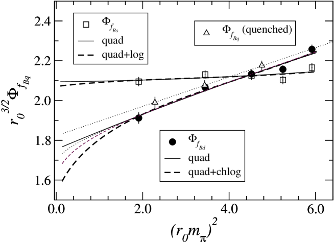
Figure 8: Chiral extrapolation of $\Phi_{f_{B_{d}}}$ (filled circles) and $\Phi_{f_{B_{s}}}$ (open squares). The quadratic extrapolation is shown by solid lines, while the fits with the hard cutoff chiral logarithm are shown for $\mu$ = 300 MeV (dotted curve), 500 MeV (thin dashed curve) and $\infty$ (thick dashed curve). Quenched results are also shown (triangles). (Figure taken from the JLQCD collaboration [172] .)

We shall use the unquenched lattice result in (110) by adding the errors in quadrature and symmetrizing the errors, getting

$$f_{B_{d}}\sqrt{\hat{B}_{B_{d}}}=210\pm 24~{}{\rm MeV}\,.$$ (111)

The dependence of $|V_{td}|$ on the various input parameters can be expressed through the following numerical formula

$$|V_{td}|=8.5\times 10^{-3}\bigg{[}\frac{210~{}{\rm MeV}}{f_{B_{d}}\sqrt{\hat{B}_{B_{d}}}}\bigg{]}\bigg{[}\frac{\Delta M_{B_{d}}}{0.50/{\rm ps}}\bigg{]}^{0.5}\sqrt{\frac{0.55}{\hat{\eta}_{B}}}\sqrt{\frac{2.40}{S_{0}(x_{t})}}\,,$$ (112)

where the default value of $S_{0}(x_{t})$ corresponds to $\overline{m_{t}}(m_{t})=167$ GeV, and the dependence of this function on $m_{t}$ [179] is $S_{0}(x_{t})\sim x_{t}^{1.52}$. To get the $\pm 1\sigma$ range for $|V_{td}|$, we vary the input parameters within their respective $\pm 1\sigma$ range and add the errors in quadrature. This exercise yields

$$|V_{td}|=(8.5\pm 1.0)\times 10^{-3}\,.$$ (113)

In future, unquenched lattice results for $f_{B_{d}}$ and other quantities will be available at smaller values of the dynamical quark masses (than is the case in the current JLQCD calculation), allowing to check the chiral logarithmic behaviour of $f_{B_{d}}$, or at least reduce the error associated with this extrapolation.

Knowing $|V_{td}|$ from (113), and $|V_{cb}|$, and $\lambda$ from previous sections, one can determine the other side of the UT, which has the following central value:

$$R_{t}\equiv\frac{1}{\lambda}\frac{|V_{td}|}{|V_{cb}|}=0.93\bigg{[}\frac{|V_{td}|}{8.5\times 10^{-3}}\bigg{]}\bigg{[}\frac{0.041}{|V_{cb}|}\bigg{]}\,.$$ (114)

Taking into account the errors (and taking symmetric errors on $|V_{td}|$), we get $R_{t}=0.93\pm 0.12$.

5.2 $|V_{td}|$ from $B\rightarrow\rho\gamma$ decays

Independent information on $|V_{td}|$ (more precisely on $\bar{\rho}$ and $\bar{\eta}$) will soon be available from the radiative decays $B\rightarrow(\rho,\omega)\gamma$. There is quite a lot of theoretical interest lately in this process, starting from the earlier papers a decade ago [180, 181], where the potential impact of these decays on the CKM phenomenology was first worked out using the leading order estimates for the penguin amplitudes. Since then, annihilation contributions have been estimated in a number of papers[182, 183, 135], and the next-to-leading order corrections to the decay amplitudes have also been calculated [155, 156]. Deviations from the SM estimates in the branching ratios, isospin-violating asymmetry $\Delta^{\pm 0}$ and CP-violating asymmetries ${\cal A}_{\rm CP}(\rho^{\pm}\gamma)$ and ${\cal A}_{\rm CP}(\rho^{0}\gamma)$ have also been worked out in a number of theoretical scenarios [184, 185, 186]. These CKM-suppressed radiative penguin decays were searched for by the CLEO collaboration [187], and the searches have been set forth at the $B$ factory experiments BELLE [188] and BABAR [189]. The current upper limits at ${90\%\ \mathrm{C.L.}}$ (averaged over the charge conjugated modes) are given in Table 1.

Table 1: $90\%$ confidence level upper limits on the branching ratios (in units of $10^{-6}$) for the decays $B\rightarrow\rho\gamma$ and $B\rightarrow\omega\gamma$ from the CLEO [187], BELLE [188] and BABAR [189] collaborations.

	${\cal B}(B^{+}\rightarrow\rho^{+}\gamma)$	${\cal B}(B^{0}\rightarrow\rho^{0}\gamma)$	${\cal B}(B^{0}\rightarrow\omega\gamma)$
CLEO (9.1 fb-1)	$13.0$	$17.0$	$9.2$
BELLE (78 fb-1)	$2.7$	$2.6$	$4.4$
BABAR (78 fb-1)	$2.1$	$1.2$	$1.0$

The BABAR upper limits on ${\cal B}(B^{+}\rightarrow\rho^{+}\gamma)$ and ${\cal B}(B^{0}\rightarrow\rho^{0}\gamma)$ have been combined using isospin symmetry to yield an improved upper limit [189]

$${\cal B}(B\rightarrow\rho\gamma)<1.9\times 10^{-6}\;.$$ (115)

Together with the current measurements of the branching ratios for $B\rightarrow K^{*}\gamma$ decays, studied earlier, this yields a ${90\%\ \mathrm{C.L.}}$ upper limit on the isospin-weighted and charge-conjugate averaged ratio [189]

$${\bar{R}}(\rho\gamma/K^{*}\gamma)\equiv\frac{{\cal B}(B\rightarrow\rho\gamma)}{{\cal B}(B\rightarrow K^{*}\gamma)}<0.047\;.$$ (116)

The branching ratios for $B\rightarrow\rho\gamma$ have been calculated in the SM at next-to-leading order [155, 156] in the QCD factorization framework [158]. As the absolute values of the form factors in this decay and in $B\rightarrow K^{*}\gamma$ decays discussed earlier are quite uncertain, it is advisable to calculate instead the ratios of the branching ratios

$$R^{\pm}(\rho\gamma/K^{*}\gamma)\equiv\frac{{\cal B}(B^{\pm}\rightarrow\rho^{\pm}\gamma)}{{\cal B}(B^{\pm}\rightarrow K^{*\pm}\gamma)},$$ (117)

$$R^{0}(\rho\gamma/K^{*}\gamma)\equiv\frac{{\cal B}(B^{0}\rightarrow\rho^{0}\gamma)}{{\cal B}(B^{0}\rightarrow K^{*0}\gamma)}.$$ (118)

The results in the NLO accuracy can be expressed as [155]:

$$R^{\pm}(\rho\gamma/K^{*}\gamma) = \left|V_{td}\over V_{ts}\right|^{2}\frac{(M_{B}^{2}-M_{\rho}^{2})^{3}}{(M_{B}^{2}-M_{K^{*}}^{2})^{3}}~{}\zeta^{2}(1+\Delta R^{\pm}(\epsilon_{\rm A}^{\pm},\bar{\rho},\bar{\eta}))\;,$$

$$R^{0}(\rho\gamma/K^{*}\gamma) = {1\over 2}\left|V_{td}\over V_{ts}\right|^{2}\frac{(M_{B}^{2}-M_{\rho}^{2})^{3}}{(M_{B}^{2}-M_{K^{*}}^{2})^{3}}~{}\zeta^{2}(1+\Delta R^{0}(\epsilon_{\rm A}^{0},\bar{\rho},\bar{\eta}))\;,$$

where $\zeta=T_{1}^{\rho}(0)/T_{1}^{K^{*}}(0)$, with $T_{1}^{\rho}(0)$ and $T_{1}^{K^{*}}(0)$ being the form factors evaluated at $q^{2}=0$ in the decays $B\rightarrow\rho\gamma$ and $B\rightarrow K^{*}\gamma$, respectively. The functions $\Delta R^{\pm}(\epsilon_{\rm A}^{\pm},\bar{\rho},\bar{\eta})$ and $\Delta R^{0}(\epsilon_{\rm A}^{0},\bar{\rho},\bar{\eta})$, appearing on the r.h.s. of the above equations encode both the $O(\alpha_{s})$ and annihilation contributions, and they have a non-trivial dependence on the CKM parameters $\bar{\rho}$ and $\bar{\eta}$ [155, 156]. Updating them, incorporating also a shift in the quantity called $\lambda_{B}^{-1}$, related to an integral over the $B$-meson LCDA, $\lambda_{B}^{-1}=\int_{0}^{\infty}dk/k~{}\phi_{+}(k,\mu)$, which has been evaluated in the QCD sum rule approach recently by Braun and Korchemsky [190], $\lambda_{B}^{-1}=(2.15\pm 0.50)$ GeV^-1, the result for the functions in (LABEL:rapp) is [161]

$$\Delta R^{\pm}=0.056\pm 0.10\,,\qquad\Delta R^{0}=-0.010\pm 0.064\,,$$ (120)

where the uncertainties reflect also the variations in the CKM parameters $\bar{\rho}$ and $\bar{\eta}$, for which the ranges $\bar{\rho}=0.21\pm 0.09$ and $\bar{\eta}=0.34\pm 0.05$ have been used.

Theoretical uncertainty in the evaluation of the ratios $R^{\pm}(\rho\gamma/K^{*}\gamma)$ and $R^{0}(\rho\gamma/K^{*}\gamma)$ is dominated by the imprecise knowledge of the quantity $\zeta$. In the SU(3) limit $\zeta=1$; SU(3)-breaking corrections have been calculated in several approaches, including the QCD sum rules and Lattice QCD. In the earlier calculations of the ratios, the following ranges were used $\zeta=0.76\pm 0.06$ (by Ali and Parkhomenko [155]), $\zeta=0.76\pm 0.10$ (Ali and Lunghi [185]) and $1/\zeta=1.33\pm 0.13$, leading to $\zeta=0.75\pm 0.07$ (Bosch and Buchalla [191]). These ranges reflect the earlier estimates of this quantity in the QCD sum rule approach [182, 192, 193, 194], and indicates substantial SU(3) breaking in the $B\rightarrow V$ form factors. Now there exists an improved Lattice estimate of this quantity, with the result [162] $\zeta=0.9\pm 0.1$, which is within $1\sigma$ compatible with no SU(3)-breaking! We conclude that $\zeta$ is at present poorly determined. It is essential to calculate it precisely if the measurement of $\bar{R}(\rho\gamma/K^{*}\gamma)$ is to make an impact on the CKM phenomenology.

To illustrate the impact of the current bound on $\bar{R}(\rho\gamma/K^{*}\gamma)$, we use the following estimate

$$\zeta=0.85\pm 0.10\,.$$ (121)

Including the uncertainties from other input parameters, the updated results are [161]

$$R^{\pm}(\rho\gamma/K^{*}\gamma) = 0.033\pm 0.012\,,$$

$$R^{0}(\rho\gamma/K^{*}\gamma) = 0.016\pm 0.006\,.$$

Combining these with the measured values of the branching ratios ${\cal B}(B^{\pm}\rightarrow K^{*\pm}\gamma)$ and ${\cal B}(B^{0}\rightarrow K^{*0}\gamma)$, the predictions for ${\cal B}(B^{\pm}\rightarrow\rho^{\pm}\gamma)$ and ${\cal B}(B^{0}\rightarrow\rho^{0}\gamma)$ are as follows:

$${\cal B}(B^{\pm}\rightarrow\rho^{\pm}\gamma) = (1.36\pm 0.49[{\rm th}]\pm 0.10[{\rm exp}])\times 10^{-6}\,,$$

$${\cal B}(B^{0}\rightarrow\rho^{0}\gamma) = (0.64\pm 0.23[{\rm th}]\pm 0.04[{\rm exp}])\times 10^{-6}\,,$$

and ${\cal B}(B^{0}\rightarrow\rho^{0}\gamma)={\cal B}(B^{0}\rightarrow\omega\gamma)$ for the stated range of theoretical uncertainty. Comparing these predictions with the present experimental bounds given in Table 1, we expect that all these branching ratios lie within a factor 2 of the current experimental bounds, and hence will be measured soon.

The isospin-weighted and charge-conjugation averaged ratio $\bar{R}(\rho\gamma/K^{*}\gamma)$ is given by the following expression in the SM [155]

$$\bar{R}(\rho\gamma/K^{*}\gamma) = \frac{\lambda^{2}\zeta^{2}}{2}\,\frac{(M_{B_{d}}^{2}-m_{\rho}^{2})^{3}}{(M_{B_{d}}^{2}-m_{K^{*}}^{2})^{3}}\,\bigg{\{}\left[1-\bar{\rho}+\varepsilon_{A}^{\pm}\bar{\rho}\right]^{2}+\left(1-\varepsilon_{A}^{\pm}\right)^{2}\bar{\eta}^{2}$$ (124)

$$+ {\rm Re}\left[G_{1}(\bar{\rho},\varepsilon_{A}^{\pm})+\bar{\eta}^{2}\,G_{2}(\varepsilon_{A}^{\pm})\right]+(\varepsilon_{A}^{\pm}\rightarrow\varepsilon_{A}^{0})\bigg{\}},$$

where the NLO contribution are introduced through the functions:

$$G_{1}(\bar{\rho},\varepsilon_{A}) = \frac{2}{C_{7}^{(0){\rm eff}}}\left\{(1-\bar{\rho})^{2}\left[A_{\rm sp}^{(1)\rho}-A_{\rm sp}^{(1)K^{*}}\right]\right.+\left.\bar{\rho}(1-\bar{\rho})\left[A^{u}+\varepsilon_{A}A^{(1)t}\right]+\bar{\rho}^{2}\varepsilon_{A}A^{u}\right\},$$

$$G_{2}(\varepsilon_{A}) = \frac{2}{C_{7}^{(0){\rm eff}}}\left\{A_{\rm sp}^{(1)\rho}-A_{\rm sp}^{(1)K^{*}}-A^{u}+\varepsilon_{A}\left[A^{u}-A^{(1)t}\right]\right\}.$$

Here, $\epsilon_{A}$ represents the annihilation contribution, estimated as $\epsilon_{A}^{\pm}\simeq 0.3\pm 0.07$ [182] with $\epsilon_{A}^{0}\ll\epsilon_{A}^{\pm}$ due to being colour- and electric charge suppressed, and the other quantities in (124) and (LABEL:auxiliar) can be seen in the literature [155].

The dependence of the ratio $\bar{R}(\rho\gamma/K^{*}\gamma)$ on $|V_{td}|/|V_{ts}|$ is shown in Fig. 9. Note, that this deviates from a quadratic dependence, which holds only if one neglects the annihilation and $O(\alpha_{s})$ corrections. Including these corrections, we have given the dependence of $\bar{R}(\rho\gamma/K^{*}\gamma)$ on $\bar{\rho}$ and $\bar{\eta}$ explicitly. The solid curve corresponds to the central values of the input parameters, and the dashed curves are obtained by taking into account the $\pm 1\sigma$ errors on the individual input parameters in $\bar{R}(\rho\gamma/K^{*}\gamma)$ and adding the errors in quadrature. The current experimental upper limit on $\bar{R}(\rho\gamma/K^{*}\gamma)$, given in (116), is also shown. Taking the least restrictive of the three theoretical curves, the current experimental upper limit yields $|V_{td}|/|V_{ts}|<0.28$, to be compared with the SM range $|V_{td}|/|V_{ts}|=0.21\pm 0.03$, shown as the region between the two dotted horizontal lines. Conversely, constraining the ratio $|V_{td}|/|V_{ts}|$ in the SM range, we get $\bar{R}(\rho\gamma/K^{*}\gamma)=0.032\pm 0.008$.

width=0.45file=RRhoKsav.eps

Figure 9: Ratio of the branching ratios for the decays $B\rightarrow\rho\gamma$ and $B\rightarrow K^{*}\gamma$, $\bar{R}(\rho\gamma/K^{*}\gamma)$, plotted as a function of $|V_{td}/V_{ts}|$. The current experimental upper limit $\bar{R}(\rho\gamma/K^{*}\gamma)<0.47$ is shown as the horizontal line. The vertical dotted lines demarcate the $\pm 1\sigma$ range of $|V_{td}/V_{ts}|$ from the SM-based unitarity fits. The solid curve corresponds to the central values of the input parameters and the dotted curves delimit the $\pm 1\sigma$ range in the NLO corrected calculations for $\bar{R}(\rho\gamma/K^{*}\gamma)$ in the SM. (Figure updated from Ref. [155].)

5.3 Present status of $|V_{ts}|$

There are two measurements at present which yield indirect information on $|V_{ts}|$, namely the lower bound on the $B_{s}^{0}$ - $\overline{B_{s}^{0}}$ mass difference $\Delta M_{B_{s}}$ and the measurement of the branching ratio ${\cal B}(B\rightarrow X_{s}\gamma)$. We discuss them in turn below.

The expression for $\Delta M_{B_{s}}$ in the SM can be obtained from the one for $\Delta M_{B_{d}}$ in (105) by the replacements: $B_{d}\rightarrow B_{s}$, $V_{td}\rightarrow V_{ts}$. However, as opposed to $\Delta M_{B_{d}}$, $\Delta M_{B_{s}}$ is not yet measured, and the current lower bound (at 95% C.L.) is [59] $\Delta M_{B_{s}}>14.4~{}{\rm(ps)}^{-1}$. This can be converted into a lower bound on $|V_{ts}|$, knowing $f_{B_{s}}\sqrt{\hat{B}_{B_{s}}}$. The unquenched lattice QCD calculation from the JLQCD Collaboration for $f_{B_{s}}$ and $f_{B_{s}}\sqrt{\hat{B}_{B_{s}}}$ yields [172]

$$f_{B_{s}} = 215(9)(^{+0}_{-2})(13)(^{+6}_{-0})~{}{\rm MeV}\,,$$

$$f_{B_{s}}\sqrt{\hat{B}_{B_{s}}} = 255(10)(^{+3}_{-2})(17)(^{+7}_{-0})~{}{\rm MeV}\,,$$

where the errors have the same origin as in (110), and the additional error here is due to the ambiguity in the determination of the $s$-quark mass. An average of the JLQCD, MILC and CP-PACS data gives [176] $f_{B_{s}}\sqrt{\hat{B}_{B_{s}}}=254\pm 13\pm 14\pm 13$ MeV. However, a recent calculation of the coupling constants $f_{B_{s}}$ and $f_{D_{s}}$ in the unquenched lattice QCD including the effects of one strange sea quark and two light sea quarks by Wingate et al. [195] yields,

$$f_{B_{s}} = 260\pm 7\pm 26\pm 8\pm 5~{}{\rm MeV}\,,$$

$$f_{D_{s}} = 290\pm 20\pm 29\pm 29\pm 6~{}{\rm MeV}\,,$$

where the errors are respectively due to statistics and fitting, perturbation theory, relativistic corrections, and discretization effects. The result for $f_{B_{s}}$ in (LABEL:wingateetal) is typically 20% higher compared to the one from the JLQCD collaboration given in (LABEL:aoki2003fbs). As both of these calculations are based on the NRQCD framework for heavy quarks, the difference between the two lies in the details of the lattice simulations, such as the dynamical quark masses used and $n_{f}$, which are different in the two approaches. Based on these comparisons, we conclude that the current lattice precision on $f_{B_{s}}\sqrt{\hat{B}_{B_{s}}}$ is of order $20\%$.

It has become customary to use the ratio of the mass differences $\Delta M_{B_{d}}/\Delta M_{B_{s}}$ to constrain $|V_{td}|/|V_{ts}|$ from the SM relation [196]:

$$\frac{\Delta M_{B_{s}}}{\Delta M_{B_{d}}}=\xi\,\frac{M_{B_{s}}}{M_{B_{d}}}\,\frac{|V_{tb}^{*}V_{ts}|^{2}}{|V_{tb}^{*}V_{td}|^{2}}\,,$$ (128)

where

$$\xi\equiv\frac{f_{B_{s}}\sqrt{\hat{B}_{B_{s}}}}{f_{B_{d}}\sqrt{\hat{B}_{B_{d}}}}\,.$$ (129)

Theoretical uncertainty in $\xi$ is arguably smaller compared to the one in $f_{B_{s}}\sqrt{\hat{B}_{B_{s}}}$, as in the SU(3) limit $\xi=1$, and the uncertainty is really in the estimate of SU(3)-breaking corrections. Thus, $\delta\xi\simeq 10\%$ is not an unrealistic error on $\xi$. Current estimates can be exemplified by the unquenched lattice calculations of $\xi$ from the JLQCD collaboration  [172]

$$\xi=1.14(3)(^{+13}_{-0})(2)(^{+3}_{-0})\,.$$ (130)

The single largest uncertainty in $\xi$ is due to the chiral extrapolation - the same source as in the estimates of $f_{B_{d}}\sqrt{\hat{B}_{B_{d}}}$. Symmetrizing the errors, JLQCD result yields

$$\xi=1.19\pm 0.09\,.$$ (131)

It should be remarked that the quantity $\Xi\equiv\xi f_{\pi}/f_{K}$ is useful to estimate $\xi$, as the chiral logs largely cancel in $\Xi$ [197]. Using the JLQCD data  [172], Kronfeld [177] quotes $\xi=1.23\pm 0.06$, with the error increasing if one includes the preliminary HPQCD results [198], yielding $\xi=1.25\pm 0.10$. The errors in this and the one in (131) are almost the same and about $8\%$. Thus, $\xi$ has a value in the range $1.1\leq\xi\leq 1.3$.

The constraint that a measurement of (or equivalently a bound on) $\Delta M_{B_{s}}$ provides on $R_{t}$ can be expressed as follows

$$R_{t}=0.90\,\bigg{[}\frac{\xi}{1.20}\bigg{]}\,\sqrt{\frac{17.3/{\rm ps}}{\Delta M_{B_{s}}}}\,\sqrt{\frac{\Delta M_{B_{d}}}{0.50/{\rm ps}}}\,,$$ (132)

where the default value of $\Delta M_{B_{s}}$ is the best-fit value from the CKM unitarity fits, discussed in detail later . The present bound $\Delta M_{B_{s}}>14.4~{}({\rm ps})^{-1}$ yields

$$\frac{|V_{td}|}{|V_{ts}|}>0.22~{}~{}\Longrightarrow~{}~{}|V_{tb}^{*}V_{ts}|>0.034\,,$$ (133)

where the last inequality follows from using $|V_{tb}^{*}V_{td}|>7.5\times 10^{-3}$, determined earlier. This is to be compared with the CKM-unitarity constraint $|V_{tb}V_{ts}^{*}|=|V_{cb}V_{cs}^{*}|+O(\lambda^{2})$, which for the central value of $|V_{cb}|=0.041$, predicts $|V_{ts}|=0.04$.

5.4 Determination of $|V_{ts}|$ from $\Gamma(B\rightarrow X_{s}\gamma)$

We now discuss the determination of $|V_{ts}|$ from ${\cal B}(B\rightarrow X_{s}\gamma)$. The effective Hamiltonian which governs the transition $B\rightarrow X_{s}\gamma$ in the SM is

$${\cal H_{\rm eff}}=-\frac{4G_{F}}{\sqrt{2}}\,V_{ts}^{*}V_{tb}\,\sum_{i=1}^{8}C_{i}(\mu)O_{i}(\mu),$$ (134)

which is obtained by integrating out all the particles that are much heavier than the $b$-quark. The operators $O_{i}$ can be seen, for example, in Ref. [199], and unitarity of the CKM matrix is used to factorize the CKM-dependence of ${\cal H_{\rm eff}}$ in the multiplicative product $V_{ts}^{*}V_{tb}$.

The decay rate for $B\rightarrow X_{s}\gamma$ is calculated by taking into account the QCD perturbative and power corrections. What concerns the perturbative corrections, there are two effects: (i) renormalization of the Wilson coefficients $C_{i}(M_{W})\rightarrow C_{i}(\mu_{b})$, where $\mu_{b}\sim O(m_{b})$, and (ii) perturbative corrections to the matrix elements of the operators $\langle O_{i}\rangle$. From step (i), one has a perturbative expansion for $C_{i}(\mu_{b})$ [200]

$$C_{i}(\mu_{b})=C_{i}^{(0)}(\mu_{b})+\frac{\alpha_{s}(\mu_{b})}{4\pi}C_{i}^{(1)}(\mu_{b})+\ldots.$$ (135)

In the leading order, i.e., without the QCD corrections, $C_{i}^{(0)}(\mu_{b})=C_{i}(M_{W})$ and $C_{i}^{(1)}(\mu_{b})=0$, and of the Wilson coefficients $C_{i}(M_{W})$ only $C_{7}(M_{W})$, corresponding to the electromagnetic penguin operator $O_{7}=em_{b}/g_{s}^{2}(\bar{s}_{L}\sigma^{\mu\nu}b_{R})F_{\mu\nu}$, is relevant for the decay $b\rightarrow s\gamma$. As $C_{7}(M_{W})$ is dominated by the (virtual) top quark contribution, the amplitude ${\cal M}(b\rightarrow s\gamma)$ is proportional to $\lambda_{t}=V_{tb}V_{ts}^{*}$. In this order, the contributions from the intermediate up and charm quarks are negligible, being power suppressed due to the GIM mechanism [3]. So, in the leading order, the decay width $\Gamma(B\rightarrow X_{s}\gamma)$ depends quadratically on $|V_{ts}^{*}V_{tb}|$.

However, including QCD corrections, the power-like GIM-suppression of the intermediate up and charm quarks is no longer operative. The reason for this is that QCD forces a very significant operator-mixing between the operator $O_{2}=(\bar{s}_{L}\gamma_{\mu}c_{L})(\bar{c}_{L}\gamma^{\mu}b_{L})$, whose Wilson coefficient $C_{2}$ is of order 1, and the electromagnetic penguin operator $O_{7}$, whose Wilson coefficient is much smaller, $C_{7}(\mu)\ll 1$. Hence the contribution from the intermediate charm state becomes numerically very important bringing with it the dependence of the decay amplitude on $\lambda_{c}=V_{cb}V_{cs}^{*}$. The contribution from the intermediate $u$-quark can always be expressed in terms of $\lambda_{t}$ and $\lambda_{c}$, using the unitarity relation $\Sigma_{u,c,t}\lambda_{i}=0$. However, on noting that $\lambda_{u}/\lambda_{t}=O(\lambda^{2})$, $\lambda_{u}$ can be dropped, to an excellent approximation, yielding $\lambda_{c}=-\lambda_{t}$, and the electromagnetic penguin amplitude $b\rightarrow s\gamma$ factorizes in $\lambda_{t}$ ($=-\lambda_{c}$).

Following this line of argument, one fixes the value of $\lambda_{t}=-\lambda_{c}=(41.0\pm 2.0)\times 10^{-3}$ in calculating the SM decay rate for $B\rightarrow X_{s}\gamma$. Thus, for example, in the $\overline{\rm MS}$ scheme, taking into account the next-to-leading order (in $\alpha_{s})$ and leading order (in $1/m_{c}^{2}$ and $1/m_{b}^{2}$) power corrections, the SM branching ratio is [76, 201]:

$${\cal B}(B\rightarrow X_{s}\gamma)=(3.70\pm 0.30)\times 10^{-4}\,,$$ (136)

to be compared with the current experimental world average (based on the CLEO, ALEPH, BELLE and BABAR measurements) of this quantity [202]

$${\cal B}(B\rightarrow X_{s}\gamma)=(3.34\pm 0.38)\times 10^{-4}\,.$$ (137)

The consistency of the two implies that the CKM unitarity, implemented through the unitarity relation

$$V_{ub}V_{us}^{*}+V_{cb}V_{cs}^{*}+V_{tb}V_{ts}^{*}=0\,,$$ (138)

holds within experimental and theoretical precision. Note, that this is a different unitarity relation than the one given in (47) and shown in Fig. 2. While it does not provide any information on the CKM parameters $\bar{\rho}$ and $\bar{\eta}$, or for that matter on $\alpha$, $\beta$ and $\gamma$, it involves the CKM matrix element $V_{ts}$, apart from the other known ones, and its best use is to determine $|V_{ts}|$ and its argument $\delta\gamma_{s}$.

We address the question how to convert the information on ${\cal B}(B\rightarrow X_{s}\gamma)$ to determine $|V_{ts}|$. To do that, we have to keep the individual contributions from the intermediate $u$, $c$ and $t$ quarks with their respective CKM dependencies, $\lambda_{u}$, $\lambda_{c}$ and $\lambda_{t}$, and not invoke unitarity, in calculating the decay width $\Gamma(B\rightarrow X_{s}\gamma)$. This is just a different book keeping of the partial contributions to the decay amplitude in the SM. Dropping small numerical contributions $(<2.5\%)$, current measurements of ${\cal B}(B\rightarrow X_{s}\gamma)$ yield the following relation [203]

$$|1.69\lambda_{u}+1.60\lambda_{c}+0.60\lambda_{t}|=(0.94\pm 0.07)|V_{cb}|\,.$$ (139)

Note the much larger coefficient of $\lambda_{c}$ compared to the coefficient of $\lambda_{t}$, reflecting the large $O_{2}$ - $O_{7}$ mixing under QCD renormalization. Note also that the relative signs of $\lambda_{c}$ and $\lambda_{t}$ are opposite, which means that a destructive interference between the charm and top quark contributions is absolutely essential to explain the observed branching ratio for $B\rightarrow X_{s}\gamma$. Solving this equation with the known values of the CKM factors, $\lambda_{c}=(41.2\pm 2.0)\times 10^{-3}$ and $\lambda_{u}$ (which is complex) from the discussions earlier (or from PDG) yields [203]

$$\lambda_{t}=V_{tb}V_{ts}^{*}=-(47\pm 8)\times 10^{-3}\,.$$ (140)

The reason for the large error on $\lambda_{t}$ is, apart from the experimental precision on ${\cal B}(B\rightarrow X_{s}\gamma)$, the relatively small coefficient of this term in (139). Within measurement errors, this determination of $\lambda_{t}$ is consistent with the CKM unitarity expectations $|V_{ts}|=|V_{cb}|+O(\lambda^{2})$, though it is less precise at present than $|V_{cb}|$. However, due to the interference of the terms proportional to $\lambda_{c}$ and $\lambda_{t}$, ${\cal B}(B\rightarrow X_{s}\gamma)$ determines the relative sign of $\lambda_{t}$ and $\lambda_{c}$. The sign in (140) is in accord with the Wolfenstein parametrization given in (4), which has $\lambda_{t}=-A\lambda^{2}$. Hence, $A$ is positive definite.

6 Summary of the Current Status of $V_{\rm CKM}$ and the Weak Phases

The current knowledge of the magnitudes of the CKM matrix elements that we have discussed in the previous sections is summarized in Table 2. Note, that these are direct measurements in the sense that unitarity has not been used in arriving at these entries. The corresponding values obtained on using the unitarity constraints are lot tighter, as also discussed above for some specific matrix elements.

Table 2: Summary of current measurements of $|V_{ij}|$.

$|V_{ij}|$	Value	$\delta|V_{ij}|/|V_{ij}|$
$|V_{ud}|$	$0.9739\pm 0.0005$	$5\times 10^{-4}$
$|V_{us}|$	$0.2224\pm 0.0020$	$9\times 10^{-3}$
$|V_{ub}|$	$(3.90\pm 0.55)\times 10^{-3}$	$14\%$
$|V_{cd}|$	$0.224\pm 0.016$	$7\%$
$|V_{cs}|$	$0.97\pm 0.11$	$11\%$
$|V_{cb}|$	$0.041\pm 0.002$	$5\%$
$|V_{td}|$	$(8.5\pm 1.0)\times 10^{-3}$	$12\%$
$|V_{ts}|$	$0.047\pm 0.008$	$17\%$
$|V_{tb}|$	$0.96^{+0.16}_{-0.23}$	$20\%$

This information can also be expressed in terms of the Wolfenstein parameters and the sides of the unitarity triangle in the SM:

$$A=0.83\pm 0.04\,,$$

$$\lambda=0.2224\pm 0.0020\,,$$

(141)

$$R_{t}=0.93\pm 0.12\,,$$

$$R_{b}=0.42\pm 0.06\,,$$

where the range of $R_{t}$ given above is coming from $\Delta M_{B_{d}}=0.503\pm 0.006$ (ps)^-1. The current lower bound on $\Delta M_{B_{s}}$ also gives a constraint on $R_{t}$, which already is quite effective in restricting the allowed $\bar{\rho}$ - $\bar{\eta}$ space in the SM. Finally, the quantity called $\bar{R}(\rho\gamma/K^{*}\gamma)$ also constrains $\bar{\rho}$ and $\bar{\eta}$, but the current upper limit is less effective than either $\Delta M_{B_{d}}$ or $\Delta M_{B_{s}}$.

So far, we have seen that the unitarity of the CKM matrix, as determined through the magnitudes of the matrix elements in each row or each column, holds with deviations which are statistically not significant. In the rest of this section, we use the information on the CP-violating asymmetries in the Kaon and $B$-meson systems to see first the consistency of the data in terms of the sides and the angles of the unitarity triangle, and then, as the final step, we undertake a fit of all the relevant data to determine the apex of the unitarity triangle shown in Fig. 2. This will allow us to update the predictions for some interesting quantities which have either not been measured yet, such as $\Delta M_{B_{s}}$, or not precisely enough, such as the angles $\alpha$ and $\gamma$.

6.1 Precise tests of the CKM theory including CP-violating phases

In addition to the constraints that we have already given in (141), (132) (for $\Delta M_{B_{s}}$), the theoretical expression for $\bar{R}(\rho\gamma/K^{*}\gamma)$ given in (124) and (LABEL:auxiliar), and the current experimental bound on this ratio in (116), there are three precise measurements involving CP violation in the $K$- and $B$-meson sectors providing constraints on the CKM parameters. We discuss them briefly here.

The observed CP-Violation in the $K_{L}\rightarrow\pi\pi$ and $K_{S}\rightarrow\pi\pi$ decays yield the following information on the quantities $|\epsilon_{K}|$ and ${\rm Re}(\epsilon^{\prime}/\epsilon)$ [2]

$$|\epsilon_{K}|=(2.280\pm 0.013)\times 10^{-3}\,,$$

(142)

$${\rm Re}(\epsilon^{\prime}/\epsilon)=(16.6\pm 1.6)\times 10^{-4}\,.$$

The value quoted for ${\rm Re}(\epsilon^{\prime}/\epsilon)$ is the world average from the NA48 [204] and KTEV [205] collaborations, including also the earlier results from their forerunners, NA31 and E731, respectively. While ${\rm Re}(\epsilon^{\prime}/\epsilon)$ is a benchmark measurement in flavour physics, as so far this is the only well established example of CP violation in decay amplitudes, unfortunately its impact on the CKM phenomenology is muted due to the imprecise knowledge of the hadronic quantities needed to extract the information on the CKM parameters quantitatively. Given the hadronic uncertainties, which admittedly are not small, the measured value of ${\rm Re}(\epsilon^{\prime}/\epsilon)$ is in agreement with the SM estimates. For further details and discussions, the interested reader is referred to a recent review on this subject by Buras and Jamin [206], where references to the original theoretical papers in the analysis of ${\rm Re}(\epsilon^{\prime}/\epsilon)$ can also be found.

Recently, time-dependent CP asymmetries in $B\rightarrow J/\psi K_{S}$ and related decays have been measured. Denoting these asymmetries generically by $a_{\psi K_{S}}(t)$, one can measure $\sin 2\beta$ (or $\sin 2\phi_{1}$) from the time dependence of the asymmetry

$$a_{\psi K_{S}}(t)\equiv a_{\psi K_{S}}\,\sin(\Delta M_{B_{d}}t)=\sin 2\beta~{}\sin(\Delta M_{B_{d}}t)\,.$$ (143)

As opposed to the theoretical predictions for $|\epsilon_{K}|$ and ${\rm Re}(\epsilon^{\prime}/\epsilon)$, the CP asymmetry $a_{\psi K_{S}}(t)$ is free of hadronic uncertainties [207], which allows to write down the above expression. Current measurements of $a_{\psi K_{S}}$ are dominated by the BABAR [208] ($a_{\psi K_{S}}=0.741\pm 0.067\pm 0.033$) and BELLE [209] ($a_{\psi K_{S}}=0.733\pm 0.057\pm 0.028$) measurements, and the world average [210, 59],

$$a_{\psi K_{S}}=0.736\pm 0.049\,,$$ (144)

is in good agreement with the predictions in the SM [2]. We shall also quantify this agreement below.

We now discuss the constraints on the CKM parameters in the SM that follow from the measurements of $|\epsilon_{K}|$ and $a_{\psi K_{S}}$. The expression for $|\epsilon_{K}|$ in the SM, including NLO corrections is [211]

$$|\epsilon_{K}|=C_{K}\,\hat{B}_{K}\,(A^{2}\lambda^{6}\bar{\eta})\,\bigg{(}x_{c}\,\left({\eta}_{3}f_{3}(x_{c},x_{t})-{\eta}_{1}\right)+{\eta}_{2}\,x_{t}\,f_{2}(x_{t})\,A^{2}\,\lambda^{4}\,(1-\bar{\rho})\bigg{)}\,,$$ (145)

where $C_{K}=G_{F}^{2}f_{K}^{2}m_{K}M_{W}^{2}/6\sqrt{2}\pi^{2}\Delta M_{K}$, with [2] $\Delta M_{K}=(3.490\pm 0.006)\times 10^{-12}$ MeV the $K^{0}$ - $\overline{K^{0}}$ mass difference and $f_{K}=(159.8\pm 1.5)$ MeV the $K$-meson coupling constant; $x_{i}=m_{i}^{2}/M_{W}^{2}$, and $f_{2}(x)$ and $f_{3}(x,y)$ are the Inami-Lim functions [168], of which we have already given $f_{2}(x)$ in (106), and $f_{3}(x,y)$ is given by the following expression (for $x\ll y$)

$$f_{3}(x,y)=\ln\frac{x}{y}-\frac{3y}{4(1-y)}\bigg{(}1+\frac{y}{1-y}\ln y\bigg{)}.$$ (146)

The ${\eta}_{i}$ are perturbative renormalization constants calculated in NLO accuracy [167, 212]. They depend on the definition of the quark masses, and the values $\eta_{2}=0.57\pm 0.01$ and $\eta_{3}=0.46\pm 0.05$ that will be used for numerical analysis below correspond to the definitions $m_{t}=m_{t}(m_{t})$ and $m_{c}=m_{c}(m_{c})$, which represent the quark masses in the $\overline{\rm MS}$ scheme at their indicated scales. With this definition, the residual $m_{t}$-dependence of $\eta_{2}$, and that of $\eta_{3}$ on $m_{t}$ and $m_{c}$, are negligible, but the dependence of $\eta_{1}$ on $m_{c}$ is significant. Following Gambino and Misiak in the CERN-CKM proceedings [9], we shall use

$$\eta_{1}=(1.32\pm 0.32)\left(\frac{1.30}{m_{c}(m_{c})}\right)^{1.1}\,,$$ (147)

and take $m_{c}(m_{c})=1.25\pm 0.1$ GeV. The quantity $\hat{B}_{K}$ is the bag parameter, for which lattice QCD estimates yield $\hat{B}_{K}=0.86(6)(14)$ [213]. In working out the constraints from $\epsilon_{K}$ numerically, we shall take $\hat{B}_{K}=0.86\pm 0.15$.

A useful numerical expression showing the constraints that the current value of $|\epsilon_{K}|$ provides on the CKM parameters is as follows [179]:

$$\bar{\eta}\left[(1-\bar{\rho})\,A^{2}\,{\eta}_{2}\,S_{0}(x_{t})+P_{c}(\varepsilon)\right]A^{2}\,\hat{B}_{K}=0.187,$$ (148)

where $S_{0}(x_{t})=x_{t}f_{2}(x_{t})\simeq 2.40\,(\bar{m}_{t}/167~{}{\rm GeV})^{1.52}$, and $P_{c}(\varepsilon)$ summarizes the contribution from the first row in (145), which depends on both $m_{c}$ and $m_{t}$. Taking into account the dependence of ${\eta}_{1}$ on $m_{c}$, this quantity is estimated as [212] $P_{c}(\varepsilon)=0.29\pm 0.07$.

Measurements of $a_{\psi K_{S}}=\sin 2\beta$ [207] translate into the following constraints on the Wolfenstein parameters

$$\sin 2\beta=\frac{2(1-\bar{\rho})\bar{\eta}}{(1-\bar{\rho})^{2}+\bar{\eta}^{2}},\qquad{\rm or}\qquad\bar{\eta}=\frac{1\pm\sqrt{1-\sin^{2}2\beta}}{\sin 2\beta}\,(1-\bar{\rho})\,.$$ (149)

The constraints resulting from the five quantities $(a_{\psi K_{S}},|\epsilon_{K}|,\Delta M_{B_{d}},\Delta M_{B_{s}}$, and $R_{b})$ on the CKM parameters $\bar{\rho}$ and $\bar{\eta}$ are shown in Fig. 10. Of these, the allowed bands correspond to $\pm 1\sigma$ errors on $a_{\psi K_{S}}$, $|\epsilon_{K}|$, $\Delta M_{B_{d}}$ and $R_{b}$, and the constraint shown for $\Delta M_{B_{s}}$ is for $\xi=1.28$, the maximum value in the $\pm 1\sigma$ range given in (131), with $\Delta M_{B_{s}}>14.4$ (ps)^-1. Of the two solutions shown for $a_{\psi K_{S}}$, only one is compatible with the measurement of $R_{b}$, i.e. with the SM, and for this solution we have a consistent description of all the data indicated in this figure; the resulting allowed region is shown as a shaded area. Note, that this is not a fit, but a simple consistency check of the CKM theory with a large number of measurements. The three dotted curves labelled as $\bar{R}(\rho\gamma/K^{*}\gamma)$ refer to the 90% C.L. bound on this ratio, and show the current theoretical uncertainty in the interpretation of this bound, which is dominated by the imprecise knowledge of $\zeta$: $\zeta=0.75$ (the leftmost curve), $\zeta=0.85$ (the central curve), and $\zeta=0.95$ (the rightmost curve).

Fig. 10 is quite instructive.

width=0.95file=EtaRho.eps

Figure 10: The constraints resulting from the measurements of $a_{\psi K_{S}}$, the ratio $R_{b}$, $\Delta M_{B_{d}}$, $\varepsilon_{K}$, and the upper bounds on $\Delta M_{B_{s}}$ and the isospin-weighted and charged-conjugate averaged ratio $\bar{R}(\rho\gamma/K^{*}\gamma)$, in the $\bar{\rho}$ - $\bar{\eta}$ plane. The overlap region is indicated by shaded area.

It shows that the knowledge of $R_{b}$ is required to distinguish between the two allowed solutions for $a_{\psi K_{S}}$. However, for the solution compatible with the SM, the allowed region in the ($\bar{\rho}$, $\bar{\eta}$) plane is now largely determined by the measurement of $a_{\psi K_{S}}$ and $\Delta M_{B_{d}}$, and the bound on $\Delta M_{B_{s}}$. The constraint from $|\epsilon_{K}|$ is still required and the compatibility of $|\epsilon_{K}|$ and $a_{\psi K_{S}}$ is an important consistency check of the CKM theory. However, as the bound on $\Delta M_{B_{s}}$ becomes stronger, more so if $\Delta M_{B_{s}}$ is measured which we anticipate soon, the allowed unitarity triangle could be determined entirely from the $B$-meson data. This is potentially good news, as the uncertainty on $\hat{B}_{K}$ is still quite substantial. This figure also reveals that the theoretical uncertainty on the ratio $\bar{R}(\rho\gamma/K^{*}\gamma)$ has to decrease by at least a factor 2 for it to be competitive with the constraints from $\Delta M_{B_{d}}$ and $\Delta M_{B_{s}}$. This requires a dedicated effort from the Lattice community, which is already under way [152]. We hope that a robust calculation of SU(3) symmetry breaking in $\zeta$ will soon be undertaken, as experiments are fast approaching the SM-sensitivity in $\bar{R}(\rho\gamma/K^{*}\gamma)$.

Table 3: Input parameters used in the CKM-unitarity fits. Values of the other parameters are taken from the recent PDG review. [2]

Parameter		Input Value
$\lambda$		$0.2224\pm 0.002~{}({\rm fixed})$
$|V_{cb}|$		$(41.2\pm 2.1)\times 10^{-3}$
$|V_{ub}|$		$(3.90\pm 0.55)\times 10^{-3}$
$a_{\psi K_{S}}$		$0.736\pm 0.049$
$|\epsilon_{K}|$		$(2.280\pm 0.13)\times 10^{-3}$
$\Delta M_{B_{d}}$		$0.503\pm 0.006~{}{\rm(ps)}^{-1}$
${\eta}_{1}(m_{c}(m_{c})=1.30~{}{\rm GeV})$		$1.32\pm 0.32$
${\eta}_{2}$		$0.57\pm 0.01$
${\eta}_{3}$		$0.46\pm 0.05$
$m_{c}(m_{c})$		$1.25\pm 0.10~{}{\rm GeV}$
$m_{t}(m_{t})$		$167\pm 5~{}{\rm GeV}$
$\hat{B}_{K}$		$0.86\pm 0.15$
$f_{B_{d}}\sqrt{B_{B_{d}}}$		$(210\pm 24)~{}{\rm MeV}$
$\eta_{B}$		$0.55\pm 0.01$
$\xi$		$1.19\pm 0.09$
$\Delta M_{B_{s}}$		$<14.4~{}{\rm(ps)}^{-1}$ at 95% C.L.

6.2 A Global fit of the CKM parameters and predictions for $\alpha$, $\gamma$ and $\Delta M_{B_{s}}$

To conclude this section, we give here the allowed ranges of the CKM-Wolfenstein parameters and the angles of the unitarity triangle obtained from a global fit of the data. Several input quantities that enter in the fits have evolved with time and their current values differ (see, Table 3) from the ones given in the CERN CKM-Workshop proceedings [9], and also from those used in the popular fits of the CKMfitter group [60]. Hence, a consistent update is not out of place.

First, a few words about the fits. We follow the Bayesian analysis method in fitting the data. However, it should be pointed out that the debate on the Bayesian vs. Non-Bayesian interpretation of data is a lively subject and it has implications for the CKM fits. In the present context the issues involved and the quantitative differences in the resulting profiles of the unitarity triangle are discussed in depth in the literature [60, 9, 214]. These differences are not crucial for our discussion, but the input values of the parameters are indeed important. To incorporate the constraint from $\Delta M_{B_{s}}$, we have used the modified-$\chi^{2}$ method (as described in the CERN CKM Workshop proceedings [215]), which makes use of the ”Amplitude Technique” introduced by Moser and Roussarie [216], in which the time-dependent oscillation probabilities are modified to have the dependence $P(B_{s}^{0}(0)\rightarrow B_{s}^{0}(t))\propto(1+{\cal A}\cos\Delta M_{B_{s}}t)$ and $P(B_{s}^{0}(0)\rightarrow\overline{B_{s}^{0}}(t))\propto(1-{\cal A}\cos\Delta M_{B_{s}}t)$. The contribution to $\chi^{2}$ of the fit from the analysis of $\Delta M_{B_{s}}$ is obtained using the following expression

$$\chi^{2}=2\,\left[{\rm Erfc}^{-1}\bigg{(}\frac{1}{2}{\rm Erfc}(\frac{1-A}{\sqrt{2}\sigma_{A}})\bigg{)}\right]^{2}\,,$$ (150)

where $A$ and $\sigma_{A}$ are the world average amplitude and the error, respectively. Relegating the details to a forthcoming publication [161], the main results are summarized below.

The constraints in the ($\bar{\rho}$,$\bar{\eta}$) plane resulting from the five individual input quantities ($R_{b}$, $\epsilon_{K}$, $\Delta M_{B_{d}}$, $\Delta M_{B_{s}}$, and $a_{\psi K_{S}}$) are shown in Fig. 11 and correspond to 95% C.L., in contrast to the ones shown in Fig. 10. The resulting 95% C.L. fit contour is shown in Fig. 11. The apex of the triangle for the best-fit solution ($\chi^{2}=0.57$ for two variables) is shown by the black dot and corresponds to the values $(\bar{\rho},\bar{\eta})=(0.17,0.36)$, with the 68% C.L. range being

$$0.11\leq\bar{\rho}\leq 0.23\,,\qquad 0.32\leq\bar{\eta}\leq 0.40\,.$$ (151)

We also show the constraint from the 90% C.L. upper bound on $\bar{R}(\rho\gamma/K^{*}\gamma)$ for the value $\zeta=0.75$, though we have not used this input in the fits. The 68% C.L. ranges of the Wolfenstein parameters $A$, $\bar{\rho}$ and $\bar{\eta}$, together with the corresponding ranges for the CP-violating phases $\alpha,\beta,\gamma$, and the mass difference $\Delta M_{B_{s}}$ are given in Table 4. Note that the fit-range for $\sin 2\beta$ coincides practically with the experimental measurement $\sin 2\beta=0.736\pm 0.049$. If we take away the input value of $\sin 2\beta$ from the fits, and instead determine $\sin 2\beta$ from the unitarity fit, we get $\sin 2\beta=0.730\pm 0.085$, which is in remarkable agreement with the experimental value, but less precise. In fact, similar estimates of $\sin 2\beta$ from the CKM unitarity constraints were obtained in the SM by several groups long before its measurements from the CP asymmetries  [217, 218, 219, 220, 221, 222]. Now, that the measurement of $a_{\psi K_{S}}$ is quite precise and its translation into $\sin 2\beta$ is free of hadronic uncertainties, this input has reduced the allowed parameter space in ($\bar{\rho},\bar{\eta})$-plane - a feature already noted in the literature [60, 185, 9, 214].

Prediction of $\Delta M_{B_{s}}$ from the fits deserves a discussion. First of all, if we take away the bound on $\Delta M_{B_{s}}$ given in Table 3 from the fits, the allowed range for $\bar{\rho}$ becomes lot larger though $\bar{\eta}$ remains essentially unchanged, yielding $0.08\leq\bar{\rho}\leq 0.27$ and $0.31\leq\bar{\eta}\leq 0.41$ at 68% C.L. The corresponding allowed range for $\Delta M_{B_{s}}$ in this case is $13.0\leq\Delta M_{B_{s}}\leq 21.6$ (ps)^-1, with the 95% C.L. interval being $[8.6,26.2]$ (ps)^-1. This range is to be compared with the corresponding one $[10.2,31.4]$ (ps)^-1 from the CKMfitter group [60]. The reason for this apparent mismatch lies in the values of the input parameters $\xi$ and $f_{B_{d}}\sqrt{B_{B_{d}}}$, for which we take the currently updated Lattice values $1.19\pm 0.09$ and $(210\pm 24)$ MeV, as opposed to the values $1.21\pm 0.04\pm 0.05$ and $(228\pm 30\pm 10)$ MeV, respectively, used by the CKMfitter group. With their input values, the resulting 95% C.L. range for $\Delta M_{B_{s}}$ from our fits becomes $[10.7,30.3]$ (ps)^-1, which is almost identical to theirs. Hence, it is important to know $\xi$ and $f_{B_{d}}\sqrt{B_{B_{d}}}$ more precisely. Including the $\Delta M_{B_{s}}$ bound in the fits, we get at 68% C.L. $14.4\leq\Delta M_{B_{s}}\leq 20.5$ (ps)^-1 with the 95% C.L. range being $[14.4,23.7]$ (ps)^-1.

Table 4: 68% C.L. ranges for the Wolfenstein parameters, CP-violating phases and $\Delta M_{B_{s}}$ from the CKM-unitarity fits.

Parameter		68% C.L. Range
$\bar{\rho}$		$0.11$ – $0.23$
$\bar{\eta}$		$0.32$ – $0.40$
$A$		$0.79$ – $0.86$
$\sin 2\beta$		$0.68$ – $0.78$
$\beta$		$21.6^{\circ}$ – $25.8^{\circ}$
$\sin 2\alpha$		$-0.44$ – $0.30$
$\alpha$		$81^{\circ}$ – $103^{\circ}$
$\sin 2\gamma$		$0.49$ – $0.95$
$\gamma$		$53^{\circ}$ – $75^{\circ}$
$\Delta M_{B_{s}}$		$14.4$ – $20.5~{}{\rm(ps)}^{-1}$

   

width=0.95file=SMfit.eps

Figure 11: Constraints on the $\bar{\rho}$ - $\bar{\eta}$ plane from the five measurements as indicated. Note that the curves labelled as $R(\rho\gamma/K^{*}\gamma)$ and $\Delta M_{B_{s}}$ are obtained from their 95% C.L. upper limits 0.047 and 14.4 (ps)^-1, respectively. The fit contour corresponds to 95% C.L., with the fitting procedure explained in the text. The dot shows the best-fit value. (Figure updated from Ref. [185].)

Concluding this section, we remark that the overall picture that has emerged from the current knowledge of the CKM parameters and hadronic quantities is that the CKM theory describes all data on flavour physics remarkably consistently, including $|\epsilon_{K}|$ and $a_{\psi K_{S}}$. Hence, it is very likely that CP violation in hadronic physics is dominated by the Kobayashi-Maskawa phase. Despite this impressive synthesis of flavour physics, a clean bill of health for the CKM theory still awaits a number of benchmark measurements. These include quantitative determination of the other two angles $\alpha$ (or $\phi_{2})$ and $\gamma$ (or $\phi_{3})$, and $\Delta M_{B_{s}}$. In all these cases, experiments have well-defined targets to shoot at, as the steady progress in the knowledge of the CKM parameters, and quite importantly the precise measurement of $\sin 2\beta$, have reduced the allowed parameter space substantially. The 95% C.L. ranges for these quantities resulting from the fits described earlier are:

$$70^{\circ}\leq\alpha\leq 114^{\circ}\,,\qquad 43^{\circ}\leq\gamma\leq 86^{\circ}\,,\qquad 14.4~{}({\rm ps})^{-1}\leq\Delta M_{B_{s}}\leq 23.7~{}({\rm ps})^{-1}\,.$$ (152)

The long run to these goal posts has already started. We anticipate significant measurements of all three within the next couple of years in experiments at the $B$ factories and Tevatron, but definitely in experiments planned at the hadron colliders (LHC-B, ATLAS, CMS and BTEV), which will measure all three angles $(\alpha,\beta,\gamma)$ accurately, as well as $\Delta M_{B_{s}}$ and a number of rare $B$-decays, such as $B_{s}\rightarrow\mu^{+}\mu^{-}$. Present situation together with some theoretical suggestions is reviewed in the next section.

7 CP Violation in $B$-Meson Decays

In the preceding section, we briefly discussed the CP asymmetries $|\epsilon_{K}|$, ${\rm Re}~{}(\epsilon^{\prime}/\epsilon)$ and $a_{\psi K_{S}}$, representing three different ways in which CP violation has been measured so far in the weak decays of the hadrons. However, CP violation is a rich and diverse phenomenon [223]. This is illustrated in Fig. 12, showing its various manifestations in the decays of a neutral meson ($P^{0}$) into a final CP eigenstate $(f_{\rm CP}$). Here, $P^{0}$ stands for any of the mesons $K^{0},D^{0},B_{d}^{0},B_{s}^{0}$.

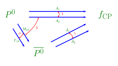
Figure 12: CP violation in neutral mesons decaying into a final CP eigenstate. Each directed line represents an amplitude with its own weak phase, and the connecting double arrows between these lines indicate possible interference patterns involving these amplitudes. (Figure taken from Nir [224])

As CP asymmetries arise due to the interference of two different amplitudes with their own weak phases, this figure shows that there are three generic manifestations of CP violation in $P^{0}$ decays.

1. Interference between the two decay amplitudes, called $A_{1}$ and $A_{2}$.

2. Interference between the mass $(M_{12})$ and width $(\Gamma_{12})$ parts of the $P^{0}$ – $\overline{P^{0}}$ mixing amplitude, giving rise to a non-vanishing relative weak phase.

3. Interference of the decay amplitudes with and without mixing, $P^{0}\rightarrow\overline{P^{0}}\rightarrow f_{\rm CP}$ and $P^{0}\rightarrow f_{\rm CP}$.

In the decays of charged mesons $P^{\pm}$ (such as $B^{\pm}$, $D^{\pm}$, $D_{s}^{\pm}$) and baryons, CP violation can take place only through the interference in the decay amplitudes.

Assuming CPT invariance, time reversal violation, or T-violation, implies CP violation. In the KM theory, CP- and T-violation have a common origin, namely the KM-phase of the CKM matrix. T-violation has been established in the $K^{0}$-$\overline{K^{0}}$ system. The measured T-violating asymmetry $A_{T}=(6.6\pm 1.0)\times 10^{-3}$ is consistent with the measurements of the CP-violating parameter $\epsilon_{K}$ [2], hence with the KM phase. T-violations have also been searched for in flavour conserving transitions. The current best upper limits on the T-violating electric dipole moments (EDMs) have been obtained for the neutron [225], Thallium-205 [226] and Mercury-199 [227]:

$$|d_{n}|<6.3\times 10^{-26}~{}{\rm e~{}cm}~{}~{}(90\%~{}{\rm C.L.})\,,$$

$$|d_{e}({\rm Tl-205})|<1.6\times 10^{-27}~{}{\rm e~{}cm}~{}~{}(95\%~{}{\rm C.L.})\,,$$ (153)

$$|d_{e}({\rm Hg-199})|<2.1\times 10^{-28}~{}{\rm e~{}cm}~{}~{}(95\%~{}{\rm C.L.})\,,$$

where the last two are to be interpreted as limits on the EDM of the electron. Judging from the current upper limit on $d_{n}$ and the prediction of the KM theory $d_{n}=O(10^{-33})$ e cm [228], T-violations in flavour conserving transitions do not provide any information on the KM phase. As a measurement of $d_{e}$ is not foreseen in the SM either, a positive result in any of the three EDMs will be a proof that additional weak phases are operative in the weak interactions of the hadrons and leptons. In particular, Supersymmetry has a myriad of weak phases, including the phases of the $A$ and $\mu$ terms, which in some parts of the supersymmetric parameter space are large enough to yield values of the EDMs of the neutron, Hg-199 and Tl-205 atoms just below the present experimental upper bound [229]. In some cases, supersymmetric weak phases will also manifest themselves in CP violation in flavour changing transitions in the $B$- and $K$-meson sectors. For example, such theories may lead to CP-violating effects in the radiative decay $B\rightarrow X_{s}\gamma$ [230]. Recent analyses incorporating the constraints from $d_{n}$ [231] predict CP asymmetry in this decay close to the current experimental bounds [232]

$${\cal A}_{\rm CP}(X_{s}\gamma) = 0.004\pm 0.051\pm 0.038\,\,\Longrightarrow-0.107\leq{\cal A}_{\rm CP}(X_{s}\gamma)\leq 0.099\,\,(90\%\,{\rm C.L.})\,,$$ (154)

$${\cal A}_{\rm CP}(K^{*}\gamma) = (-0.5\pm 3.7)\%\,\,\Longrightarrow-0.066\leq{\cal A}_{\rm CP}(K^{*}\gamma)\leq 0.056\,\,(90\%\,{\rm C.L.})\,.$$ (155)

The bounds on ${\cal A}_{\rm CP}(K^{*}\gamma)$ are stronger but they still allow this CP asymmetry to be of $O(5\%)$, much larger than the SM-based expectations [233, 234] $|{\cal A}_{\rm CP}(X_{s}\gamma)|\leq 0.5\%$. It is entirely conceivable that precision studies of CP violation in $B$- and $K$-decays may require the intervention of some of the weak phases in supersymmetric theories. The search for non-KM weak phases is an important part of the research programme at the $B$-factories and later at the hadron colliders and has to be pursued vigorously. However, we will not discuss these scenarios here, as the principal focus of this review is on the CKM phenomenology and current data show no significant deviations from the CKM theory.

In this section, we first discuss each of the three classes of CP asymmetries depicted in Fig. 12 and define the underlying physical quantities which are being sensitively probed in each one of them. This will be followed by a summary of the existing results on CP asymmetries from BABAR and BELLE in some of the main decay modes of interest for our discussion, such as $J/\psi K_{S},\phi K_{S},\eta^{\prime}K_{S},\pi\pi,K\pi$. In the SM, these asymmetries provide information on the weak phases $\alpha,\beta,\gamma$ (or $\phi_{1},\phi_{2},\phi_{3}$), and we review their current knowledge from the $B$-factory experiments.

7.1 CP violation in decay amplitudes

As opposed to $K$-mesons, direct CP violation in the $B$-meson sector is potentially a very prolific phenomenon as the number of decay channels available in the latter is enormous [235]. In practice, however, measuring some of these asymmetries, which are estimated at several percent or somewhat higher level [236] in decay modes with typical branching ratios of order $10^{-5}$, requires $O(10^{9})$ $B\bar{B}$ pairs (or more). With the present integrated luminosity of $O(10^{8})$ $B\bar{B}$ mesons recorded by the BABAR and BELLE detectors, there are now indications in the data that these experiments are observing the first direct CP asymmetry in $B$ decays. The case in point is ${\cal A}_{\rm CP}(K^{+}\pi^{-})=(-9.5\pm 2.9)\%$ [59] having a 3$\sigma$ significance.

To study direct CP asymmetry, we note that unitarity can be used to write the decay amplitudes $A(B\rightarrow f)$ and its CP-conjugate $A(\bar{B}\rightarrow\bar{f})$ as:

$$A(B\rightarrow f) = |A_{1}|{\rm e}^{+i\theta_{1}}{\rm e}^{+i\delta_{1}}+|A_{2}|{\rm e}^{+i\theta_{2}}{\rm e}^{+i\delta_{2}}\,,$$

$$A(\bar{B}\rightarrow\bar{f}) = |A_{1}|{\rm e}^{-i\theta_{1}}{\rm e}^{+i\delta_{1}}+|A_{2}|{\rm e}^{-i\theta_{2}}{\rm e}^{+i\delta_{2}}\,,$$

where $\theta_{1}$ and $\theta_{2}$ are the weak phases, and the strong interaction amplitudes $|A_{i}|{\rm e}^{+i\delta_{i}}$ $(i=1,2)$ contain the CP-conserving strong phases $\delta_{i}$. With the help of these amplitudes, the CP-rate asymmetry can be written as

$${\cal A}_{\rm CP}(f)\equiv\frac{\Gamma(\bar{B}\rightarrow\bar{f})-\Gamma(B\rightarrow f)}{\Gamma(\bar{B}\rightarrow\bar{f})+\Gamma(B\rightarrow f)}=\frac{2|A_{1}||A_{2}|\sin(\delta_{1}-\delta_{2})\sin(\theta_{1}-\theta_{2})}{|A_{1}|^{2}+2|A_{1}||A_{2}|\cos(\delta_{1}-\delta_{2})\cos(\theta_{1}-\theta_{2})+|A_{2}|^{2}}\,.$$ (157)

The goal is to extract the weak phase difference $\theta\equiv\theta_{1}-\theta_{2}$ from the measured partial rate asymmetries, for which knowledge of the strong interaction amplitudes $|A_{1}|$, $|A_{2}|$ and the strong-phase difference $\delta\equiv\delta_{1}-\delta_{2}$ is essential. The required strong phase difference involving a tree and penguin amplitudes $\delta=\delta_{P}-\delta_{T}$, or involving two penguin amplitudes with different strong phases $\delta=\delta_{P}-\delta_{P^{\prime}}$, are generated by the so-called Bander-Silverman-Soni mechanism [237]. In addition, final state interactions also generate strong phases, which have to be estimated or measured.

From the CP-averaged decay rate $(\Gamma(B\rightarrow f)+\Gamma(\bar{B}\rightarrow\bar{f}))/2$ and the CP asymmetry ${\cal A}_{\rm CP}(f)$, one has two equations with four unknowns which we take as $r\equiv|A_{2}|/|A_{1}|$, $\delta$, $\theta$, and $|A_{1}|$, with $r<1$. Hence, one has to use additional experimental input and assumptions. For the decays $B\rightarrow h_{1}h_{2}$, with $h_{i}$ belonging to a $U(3)$ nonet of (usually vector or pseudoscalar) mesons, an approximate SU(3) symmetry is invoked which allows to express $|A_{1}|$ in terms of a known branching ratio dominated by this amplitude. This then leaves only three unknowns with two constraints, which is still not sufficient to determine all the parameters, but allows to derive bounds on the weak phase $\theta$ which could be useful if data is benevolent.

While the phenomenology of direct CP violation is rich [236], a theoretically robust description is difficult and not yet at hand. Determining the weak phases from the observed asymmetries and decay rates requires a good control over the ratios of the amplitudes $|A_{P}/A_{T}|$, $|A_{P^{\prime}}/A_{T}|$, and $|A_{P}/A_{P^{\prime}}|$ etc., and the corresponding strong-phase differences $\delta_{P}-\delta_{T}$, $\delta_{P^{\prime}}-\delta_{T}$ and $\delta_{P}-\delta_{P^{\prime}}$, where we are assuming that there are two different penguin amplitudes, one generated by the exchange of gluons and the other by electroweak bosons ($\gamma$ and $Z$). Of course, direct CP asymmetries also arise when two different tree amplitudes interfere, such as in $A_{\rm CP}(DK)$. Anyway, calculating them from first principles with a non-perturbative technique, such as Lattice QCD, is simply not on the cards, as the amplitudes $|A_{i}|{\rm e}^{i\delta_{i}}$ depend on $\langle h_{1}h_{2}|{\cal O}|B\rangle$, where ${\cal O}$ is a four-quark operator. We know all too well that the vengeance of strong interactions is merciless in the analysis of ${\rm Re}(\epsilon^{\prime}/\epsilon)$ in $K$-meson decays involving the matrix elements $\langle\pi\pi|{\cal O}|K_{L,S}\rangle$, which has hindered the extraction of any information on the CKM parameters from this measurement.

One would like to argue that strong interaction effects are tractable in $B$-decays due to the large mass of the $b$-quark, and hence calculable using techniques based on $1/m_{b}$-expansion and perturbative QCD [158, 238]. However, the dynamical scale in $B\rightarrow h_{1}h_{2}$ decays is not set by the inverse $b$-quark mass, $1/m_{b}$, but by a lower value, of order $1$ -$2$ GeV - the typical virtuality of a gluon nested somewhere in the Feynman diagrams. This raises the question if perturbative methods are adequate at such low scales. Jury is still out on this issue, but when the jury returns one should not be surprised at an unfavourable verdict for the perturbative-QCD inspired factorization models.

Some help in extracting the weak phases from data can certainly be sought by using arguments based on the isospin and flavour SU(3) symmetries. The most celebrated use of the isospin symmetry is in the extraction of the phase $\alpha$ (or $\phi_{2})$ from the $B\rightarrow\pi\pi$ decays [239]. While isospin is a good symmetry, there are still missing experimental links to complete the chain of arguments to determine the weak phase $\alpha$ in a model-independent way. However, use of the SU(3) symmetry is more problematic. We have seen that the issue of SU(3)-breaking in simpler quantities, such as the ratios $\xi$ and $\zeta$, is far from being settled. In the much more complicated situation in non-leptonic decays, SU(3) symmetry breaking effects are at best modeled, often based on the assumed properties of the factorized amplitudes. This lack of a robust theoretical basis and/or data introduces hadronic uncertainties in the extraction of the weak phases from data. We shall discuss applications of these methods in the context of $B\rightarrow\pi\pi$ and $B\rightarrow K\pi$ decays to quantify some of the issues involved.

7.2 Indirect CP violation involving $B^{0}$ - $\overline{B^{0}}$ mixing amplitudes

Indirect CP asymmetries involve an interference between the absorptive and dispersive parts of the amplitudes in the $B_{d}^{0}$ - $\overline{B_{d}^{0}}$ and $B_{s}^{0}$ - $\overline{B_{s}^{0}}$ mixings. Their experimental measures are the charge asymmetries ${\cal A}_{\rm SL}(B_{d}^{0})$ and ${\cal A}_{\rm SL}(B_{s}^{0})$:

$${\cal A}_{\rm SL}(B^{0}) \equiv \frac{\Gamma(\overline{B^{0}}\rightarrow\ell^{+}X)-\Gamma(B^{0}\rightarrow\ell^{-}X)}{\Gamma(\overline{B^{0}}\rightarrow\ell^{+}X)+\Gamma(B^{0}\rightarrow\ell^{-}X)}=\frac{1-|q/p|^{4}}{1+|q/p|^{4}}\,,$$ (158)

where the ratio $q/p$ is defined as follows

$$\left(\frac{q}{p}\right)^{2}\equiv\frac{2M_{12}^{*}-i\Gamma_{12}^{*}}{2M_{12}-i\Gamma_{12}}\,,$$ (159)

and the off-diagonal elements $M_{12}$ and $\Gamma_{12}$ govern the mass difference ($\Delta M_{B}$) and the width-difference ($\Delta\Gamma_{B}$) between the two mass eigenstates, respectively. Thus,

$${\cal A}_{\rm SL}(B_{d}^{0})={\rm Im}\bigg{(}\frac{\Gamma_{12}(B_{d})}{M_{12}(B_{d})}\bigg{)}\,,\qquad{\cal A}_{\rm SL}(B_{s}^{0})={\rm Im}\bigg{(}\frac{\Gamma_{12}(B_{s})}{M_{12}(B_{s})}\bigg{)}\,.$$ (160)

Parameterizing the ratio $\Gamma_{12}(B_{q})/M_{12}(B_{q})=r_{q}e^{i\zeta_{q}}$, SM estimates are

$${\cal A}_{\rm SL}(B_{d}^{0})=r_{d}\sin\zeta_{d}\simeq{\cal O}(10^{-3})\,,\qquad{\cal A}_{\rm SL}(B_{s}^{0})=r_{s}\sin\zeta_{s}\simeq{\cal O}(10^{-4})\,.$$ (161)

Present measurements yield [59] ${\cal A}_{\rm SL}(B_{d}^{0})=(0.1\pm 1.4)\times 10^{-2}$. The bound on ${\cal A}_{\rm SL}(B_{d}^{0})$ does not probe the SM, but constrains some beyond-the-SM (BSM) scenarios [240]. Combining the data on the direct CP asymmetry ${\cal A}_{\rm CP}(B^{+}\rightarrow J/\psi K^{+})$, one can get an improved bound on $|q/p|$ [224], and we shall discuss it later. However, for all practical purposes discussed here, one can set $|q/p|=1$ for the $B_{d}^{0}$ -$\overline{B_{d}^{0}}$ system. Currently, there is no experimental bound on ${\cal A}_{\rm SL}(B_{s}^{0})$.

It is worth pointing out that the analogue of the charge asymmetry (158) in the $K^{0}$ - $\overline{K^{0}}$ system, namely the CP-violating asymmetry in the semileptonic decays $K_{L}\rightarrow\pi^{\pm}\ell^{\mp}\nu_{\ell}$, defined as,

$$\delta_{\ell}\equiv\frac{\Gamma(K_{L}\rightarrow\pi^{-}\ell^{+}\nu_{\ell})-\Gamma(K_{L}\rightarrow\pi^{+}\ell^{-}\nu_{\ell})}{\Gamma(K_{L}\rightarrow\pi^{-}\ell^{+}\nu_{\ell})+\Gamma(K_{L}\rightarrow\pi^{+}\ell^{-}\nu_{\ell})}\,,$$ (162)

is a well measured quantity [2] $\delta_{\ell}=(3.27\pm 0.12)\times 10^{-3}$. This value is consistent with the relation $\delta_{\ell}=2{\rm Re}(\epsilon_{K})/(1+|\epsilon_{K}|^{2})\simeq 2{\rm Re}(\epsilon_{K})$, and the experimental value [2] of ${\rm Re}(\epsilon_{K})$. Hence, the asymmetry $\delta_{\ell}$ arises entirely from the imaginary part of $M_{12}(K)$, which in the SM is given by ${\rm Im}(V_{ts}^{*}V_{td})$.

Current and planned experiments at the $e^{+}e^{-}$ and hadronic $B$ factories are not anticipated to reach the SM-sensitivity in ${\cal A}_{\rm SL}(B_{d}^{0})$ (even less so in ${\cal A}_{\rm SL}(B_{s}^{0})$), and, hence, a measurement of any of these asymmetries will be a sure signal of BSM physics.

7.3 Interplay of mixing and decays of $B^{0}$ and $\overline{B^{0}}$ to CP eigenstates

As already mentioned, this class of CP asymmetries involves an interference between the decays $B^{0}\rightarrow f_{\rm CP}$ and $B^{0}\rightarrow\overline{B^{0}}\rightarrow f_{\rm CP}$. Due to mixing these CP asymmetries are time-dependent, and the two time-dependent functions $\cos(\Delta M_{B}t)$ and $\sin(\Delta M_{B}t)$ can be measured, allowing to extract their coefficients $C_{f}$ and $S_{f}$, respectively:

$${\cal A}_{\rm fCP}(t)\equiv\frac{\Gamma(\overline{B^{0}}(t)\rightarrow f)-\Gamma(B^{0}(t)\rightarrow f)}{\Gamma(\overline{B^{0}}(t)\rightarrow f)+\Gamma(B^{0}(t)\rightarrow f)}=-C_{f}\cos(\Delta M_{B}t)+S_{f}\sin(\Delta M_{B}t)\,,$$ (163)

where

$$C_{f}=-{\cal A}_{f}=\frac{1-|\lambda_{f}|^{2}}{1+|\lambda_{f}|^{2}}\,,\qquad S_{f}=\frac{2{\rm Im}\lambda_{f}}{1+|\lambda_{f}|^{2}}\,,$$ (164)

and the dynamical quantity $\lambda_{f}$ is given by:

$$\lambda_{f}=(q/p)\bar{\rho}(f)\,;\qquad\bar{\rho}(f)=\frac{\bar{A}(f)}{A(f)}\,.$$ (165)

Concentrating now on $B_{d}^{0}$ and $\overline{B_{d}^{0}}$ decays, the amplitudes $A(f)$, $\bar{A}(f)$ and $q/p$ are defined as follows [2]:

$$A(f)=\langle f|H|B_{d}^{0}\rangle\,;\qquad\bar{A}(f)=\langle f|H|\overline{B_{d}^{0}}\rangle\,;\qquad q/p=\frac{V_{tb}^{*}V_{td}}{V_{tb}V_{td}^{*}}={\rm e}^{-2i\phi_{\rm mixing}}={\rm e}^{-2i\beta}\,.$$ (166)

If only a single decay amplitude is dominant, then one can write:

$$\bar{\rho}(f)=\eta_{f}{\rm e}^{-2i\phi_{\rm decay}}\qquad\Rightarrow~{}~{}|\bar{\rho}(f)|=1\,,$$ (167)

where $\eta_{f}=\pm 1$ is the intrinsic CP-Parity of the state $f$. In this case, $|\lambda_{f}|=1$, and one has

$$S_{f}={\rm Im}(\lambda_{f})=-\eta_{f}\sin 2(\phi_{\rm mixing}+\phi_{\rm decay})\,,~{}~{}C_{f}=0\,,$$ (168)

and the CP asymmetry ${\cal A}_{\rm fCP}$ has a very simple interpretation:

$${\cal A}_{\rm fCP}(t)=S_{f}\sin(\Delta M_{B}t)\,.$$ (169)

If, in addition, $\phi_{\rm decay}=0$, which is the case for the transitions $b\rightarrow c\bar{c}s$, $b\rightarrow s\bar{s}s$ and $b\rightarrow d\bar{d}s$, then a measurement of $S_{f}$ is a measurement of $\sin 2\theta_{\rm mixing}$ (modulo the sign $-\eta_{f}$). The current thrust of the BABAR and BELLE experiments in CP asymmetry measurements is indeed in extracting $S_{f}$ and $C_{f}$ for a large number of final states.

7.4 Current status of CP asymmetries in $b\rightarrow c\bar{c}s$ and $b\rightarrow s\bar{s}s$ decays

We now discuss the coefficients $S_{f}$ and $C_{f}$ for $f=J/\psi K_{S},\phi K_{S},\eta^{\prime}K_{S},K^{+}K^{-}K_{S}$. Current data on these and some other final states are summarized in Table 5. The values quoted for $f=J/\psi K_{S}$ are averages over several decay modes of the quark decay $b\rightarrow c\bar{c}s$ and include also the final states $J/\psi K_{L}$ and $J/\psi K^{*}$, with the latter angular momentum analyzed into states with well-defined CP-parities and taking into account the intrinsic CP-parity, and some other related states [210]. Also, the state $K^{+}K^{-}K_{S}$ is not a CP eigenstate and an angular analysis like the one carried out for the $B\rightarrow J/\psi K^{*}$ case has not yet been undertaken due to limited statistics. However, using arguments based on branching ratios of related modes, BELLE collaboration [241] concludes that the $K^{+}K^{-}K_{S}$ state is predominantly a CP-even eigenstate, with a fraction $1.03\pm 0.15\pm 0.05$.

In the SM, $S_{J/\psi K_{S}}$ and $C_{J/\psi K_{S}}$ are determined by the tree amplitude $b\rightarrow c\bar{c}s$ with the penguin amplitude suppressed by $\lambda^{2}$. In any case, both the $T$ and $P$ amplitudes have the same phase, and hence in the SM $S_{J/\psi K_{S}}=\sin 2\beta$ (or $\sin 2\phi_{1})$ and $C_{J/\psi K_{S}}=0$ (or $|\lambda_{J/\psi K_{S}}|=1$). Comparison of $S_{J/\psi K_{S}}$ with the indirect estimates of the same discussed earlier shows that the agreement with the SM expectations in this decay mode holds quantitatively. This is a great triumph for the KM mechanism of CP violation.

The present measurement $C_{J/\psi K_{S}}=0.052^{+0.048}_{-0.046}$ is in agreement with no direct CP violation in the decays $B^{\pm}\rightarrow J/\psi K^{\pm}$. The current bound [59]

$${\cal A}_{\rm CP}(B^{+}\rightarrow J/\psi K^{+})=\frac{|\bar{A}/A|^{2}-1}{|\bar{A}/A|^{2}+1}=-0.007\pm 0.019\,,$$ (170)

yields $|\bar{A}/A|=0.993\pm 0.018$. Combined with $|q/p|=0.9996^{+0.0068}_{-0.0067}$ from $A_{\rm SL}(B_{d}^{0})$, this yields $|\lambda_{J/\psi K_{S}}|=0.992\pm 0.019$, in precise agreement with $|\lambda_{J/\psi K_{S}}|=1$.

Going down the entries in Table 5, we note that the final states $\phi K_{S}$ and $K^{+}K^{-}K_{S}$ are determined by the penguin transition $b\rightarrow s\bar{s}s$, which has the weak phase $\pi$. The final state $\eta^{\prime}K_{S}$ receives contributions both from the penguin $b\rightarrow s\bar{s}s$ and $b\rightarrow s\bar{d}d$ amplitudes and the tree amplitude $b\rightarrow u\bar{u}s$, due to the $u\bar{u}$ content of the $\eta^{\prime}$-meson wave function. The tree amplitude, however, is CKM suppressed. So, to a good approximation, also this final state is dominated by the penguin transitions $b\rightarrow s\bar{s}s$ and $b\rightarrow s\bar{d}d$, and has the weak phase $\pi$ in the decay amplitude. Thus, in the SM, we expect that for these decays ($f=J/\psi K_{S},\phi K_{S},\eta^{\prime}K_{S},K^{+}K^{-}K_{S}$)

$$-\eta_{f}S_{f}=\sin 2\beta\,,\qquad C_{f}=0\,.$$ (171)

The current measurements of $S_{f}$ and $C_{f}$ are summarized in Table 5.

Table 5: The coefficients $S_{f}$ and $C_{f}=-{\cal A}_{f}$ from time-dependent CP asymmetry ${\cal A}_{\rm fCP}(t)$, taken from the HFAG listings [59] [BE(BA) stands for a BELLE (BABAR) entry].

$S_{f}$		$C_{f}$
$S_{J/\psi K_{S}}=0.736\pm 0.049$		$C_{J/\psi K_{S}}=0.052^{+0.048}_{-0.046}$
$S_{\phi K_{S}}=-0.14\pm 0.33$		$C_{\phi K_{S}}=-0.04\pm 0.24$
$S_{\eta^{\prime}K_{S}}=+0.27\pm 0.21$		$C_{\eta^{\prime}K_{S}}=0.04\pm 0.13$
$S_{K^{+}K^{-}K_{S}}[{\rm BE}]=-0.51\pm 0.26\pm 0.05$		$C_{K^{+}K^{-}K_{s}}[{\rm BE}]=0.17\pm 0.16\pm 0.05$
$S_{J/\psi\pi^{0}}=-0.40\pm 0.33$		$C_{J/\psi\pi^{0}}=0.13\pm 0.24$
$S_{D^{*}\overline{D^{*}}}[{\rm BA}]=0.06\pm 0.37\pm 0.13$		$C_{D^{*}\overline{D^{*}}}[{\rm BA}]=0.28\pm 0.23\pm 0.02$
$S_{+-}(D^{*+}D^{-})[{\rm BA}]=-0.82\pm 0.75\pm 0.14$		$C_{+-}(D^{*+}D^{-})[{\rm BA}]=-0.47\pm 0.40\pm 0.12$
$S_{-+}(D^{*-}D^{+})[{\rm BA}]=-0.24\pm 0.69\pm 0.12$		$C_{-+}(D^{*-}D^{+})[{\rm BA}]=-0.22\pm 0.37\pm 0.10$
$S_{\pi\pi}=-0.58\pm 0.20$		$C_{\pi\pi}=-0.38\pm 0.16$

The data are from BELLE [241] and BABAR [242], updated by Browder [210] at the Lepton-Photon Conference and the Summer 2003 updates by HFAG [59]. Note that $\eta_{J\psi K_{S}}=\eta_{\phi K_{S}}=\eta_{\eta^{\prime}K_{S}}=-1$, but $\eta_{K^{+}K^{-}K_{S}}=+1$ due to the dominance of the $CP=+1$ eigenstate in this mode. One sees that within the experimental errors, SM predictions $C_{f}=0$ for the final states specified in (171) are in agreement with the data, though the errors in the individual modes are still quite large. On the other hand, $S_{\phi K_{S}}$ and to a lesser extent also $S_{\eta^{\prime}K_{S}}$, appear to be out of line with the SM expectations (171). However, it should be noted that the two experiments BABAR and BELLE are not consistent with each other [210, 241], with $S_{\phi K_{S}}({\rm BELLE})=-0.96\pm 0.50^{+0.09}_{-0.11}$ and $S_{\phi K_{S}}({\rm BABAR})=+0.45\pm 0.43\pm 0.07$, differing by 2.1$\sigma$. Following the PDG rules [2], one has to scale the error in $S_{\phi K_{S}}$ given in Table 5 by this factor, yielding $S_{\phi K_{S}}=-0.14\pm 0.69$, which is only $1.3\sigma$ away from $S_{J/\psi K_{S}}=0.736\pm 0.049$, and hence the difference between the two is not all that compelling.

As the current statistics is low, it is helpful to combine the three ($b\rightarrow s\bar{s}s)$ penguin-dominated final states. Defining $-\eta_{f}S_{f}\equiv\sin 2\beta_{\rm eff}$, and averaging over the three final states gives [59]

$$\langle\sin 2\beta_{\rm eff}\rangle = 0.24\pm 0.15~{}~{}({\rm C.L.}=0.11)\,,$$

$$\langle C_{\rm eff}\rangle = 0.07\pm 0.09~{}~{}({\rm C.L.}=0.76)\,.$$

The two experiments (BABAR and BELLE) are still hardly compatible with each other in $\langle\sin 2\beta_{\rm eff}\rangle$; in contrast the measurements of $\langle C_{\rm eff}\rangle$ are quite consistent. The current average of $\langle C_{\rm eff}\rangle$ within errors also agrees with the corresponding quantity measured in the $b\rightarrow c\bar{c}s$ transitions, with $C_{J/\psi K_{S}}-\langle C_{\rm eff}\rangle=0.018\pm 0.10$. However, the current measurements yield [210, 59]

$$\sin 2\beta-\langle\sin 2\beta_{\rm eff}\rangle=0.50\pm 0.16\,,$$ (173)

which is a 3.1$\sigma$ effect on the face value. Taking into account the scale factor in $\langle\sin 2\beta_{\rm eff}\rangle$ increases the error, yielding $\sin 2\beta-\langle\sin 2\beta_{\rm eff}\rangle=0.50\pm 0.25$, which differs from 0 by $2\sigma$. This difference is more significant than $S_{J/\psi K_{S}}-S_{\phi K_{S}}$, but still does not have the statistical weight to usher us into a new era of CP violation. We have to wait for more data.

While there are already quite a few suggestions in the recent literature explaining the difference $S_{\phi K_{S}}-S_{J/\psi K_{S}}$ in terms of physics beyond the SM, we will not discuss them as the experimental significance of the effect is marginal. However, a more pertinent question to ask is: How well are the SM equalities given in (171) satisfied? This point has been investigated recently by Grossman et al. [243]. Following their notation, the SM amplitudes in these decays can be parametrized as:

$$A_{f}\equiv A(B^{0}\rightarrow f)=V_{cb}^{*}V_{cs}a_{f}^{c}+V_{ub}^{*}V_{us}a_{f}^{u}\,,$$ (174)

where $a_{f}^{c}$ is dominated by the $b\rightarrow s\bar{s}s$ gluonic penguin diagrams and $a_{f}^{u}$ gets contributions from both penguin and $b\rightarrow u\bar{u}s$ tree diagrams. The second term is CKM-suppressed compared to the first:

$${\rm Im}\left(\frac{V_{ub}^{*}V_{us}}{V_{cb}^{*}V_{cs}}\right)=\left|\frac{V_{ub}^{*}V_{us}}{V_{cb}^{*}V_{cs}}\right|\sin\gamma=O(\lambda^{2})\sin\gamma\,.$$ (175)

It is conceivable though not very likely that the CKM-suppression is offset by a dynamical enhancement of the ratio $a_{f}^{u}/a_{f}^{c}$. Note that $|a_{f}^{u}/a_{f}^{c}|\sim 1$ (from penguins), but $|a_{f}^{u}/a_{f}^{c}|$ (from tree) could be $\gg 1$. To quantify this, Grossman et al. [243] define

$$\xi_{f}\equiv\frac{V_{ub}^{*}V_{us}a_{f}^{u}}{V_{cb}^{*}V_{cs}a_{f}^{c}}~{}\Rightarrow~{}A_{f}=V_{cb}^{*}V_{cs}a_{f}^{c}(1+\xi_{f})\,.$$ (176)

SU(3) allows to put bounds on $|\xi{{}_{f}}|$:

$$-\eta_{f}S_{f}-\sin 2\beta = 2\cos 2\beta\sin\gamma\cos\delta_{f}|\xi_{f}|\,,$$

$$C_{f} = -2\sin\gamma\sin\delta_{f}|\xi_{f}|\,,$$

where $\delta_{f}={\rm arg}(a_{f}^{u}/a_{f}^{c})$ and $\xi_{f}$ also characterizes the size of $C_{f}$. Note that $\delta_{f}$ can be determined from $\tan\delta_{f}=(\eta_{f}S_{f}+\sin 2\beta)/(C_{f}\cos 2\beta)$. However, present bounds are not very restrictive due to lack of information on some decays and additional assumptions are required to be more quantitative. Typical estimates are [243]:

$$|\xi_{\eta^{\prime}K_{S}}| < 0.36~{}~{}[{\rm SU(3)}];~{}~{}0.09~{}~{}[{\rm SU(3)}+{\rm Leading}~{}N_{c}]\,,$$

$$|\xi_{\phi K_{S}}| < 0.25~{}~{}[{\rm SU(3)}+{\rm Non-cancellation}]\,,$$ (178)

$$|\xi_{K^{+}K^{-}K_{S}}| < 0.13~{}~{}[U-{\rm Spin}]\,,$$

where the various assumptions in arriving at the numerical inequalities have been specified. More data and further theoretical analysis are required to further restrict $|\xi_{f}|$ in a model-independent way. Hence, at this stage, one should use values of $\xi_{f}$ indicated in (178).

7.5 Current status of the CP asymmetries in $b\rightarrow c\bar{c}d$ decays

CP asymmetries in some of the final states which are induced by the transition $b\rightarrow c\bar{c}d$ have also been studied by the BABAR and BELLE collaborations. The coefficients $S_{f}$ and $C_{f}$ for $f=J/\psi\pi^{0},~{}D^{*}\overline{D^{*}},~{}D^{*+}D^{-},~{}D^{*-}D^{+}$ measured through the time-dependent CP-asymmetry in these channels are given in the lower part of Table 5. Note that the entry for $f=J/\psi\pi^{0}$ is the average of the BABAR [244] and BELLE [245] experiments, but the entries for $f=D^{*+}D^{-},~{}f=D^{*-}D^{+}$ and $f=D^{*}\overline{D^{*}}$ are from the BABAR collaboration [246, 247] alone with the BELLE results not yet available. Just like the $b\rightarrow c\bar{c}s$ case, the tree amplitude in the $b\rightarrow c\bar{c}d$ transition does not have a weak phase. However, as opposed to the $b\rightarrow c\bar{c}s$ case, where the penguin amplitude has the weak phase $\pi$, now there could be a non-negligible contribution from the $b\rightarrow d$ penguin amplitude, which carries the weak phase $\beta$. In terms of the CKM factors, both the T and P amplitudes are of order $\lambda^{3}$. The tree-penguin interference with different weak phases may lead to direct CP violation, giving rise to $C_{f}\neq 0$, or $|\lambda_{f}|\neq 1$. Also, in this case, the equality $-S_{J/\psi\pi^{0}}=S_{J/\psi K_{S}}$ or $-S_{D^{*}\overline{D^{*}}}(+)=S_{J/\psi K_{S}}$ etc. can be violated. Here the sign$(+)$ stands for the CP$=+1$ component of the Vector-Vector final state, which for $D^{*}\overline{D^{*}}$ dominates the decay, with the CP-odd component given by [247] $R_{\perp}=D^{*}\overline{D^{*}}({\rm P~{}wave})/D^{*}\overline{D^{*}}=0.063\pm 0.055\pm 0.009$. Present data are consistent with the SM and no direct CP violation in these decays is observed. Also, the measured coefficients $S_{f}$ for these decays do not show significant deviations from the SM expectations (ignoring penguins) $-\eta_{f}S_{f}=S_{J/\psi K_{S}}$. This brings us to the entry in the last row in Table 5 for $f=\pi\pi$, which we discuss below together with the two methods most discussed in the literature to determine the angle $\alpha$ (or $\phi_{2}$).

7.6 Measurements of the weak phase $\alpha$ (or $\phi_{2})$ in $B$-meson decays

In the previous section we have given the 95% C.L. range for the weak phase $\alpha$ obtained from the CKM unitarity fits: $70^{\circ}\leq\alpha\leq 115^{\circ}$. This phase will be measured through CP violation in the $B\rightarrow\pi\pi$ and $B\rightarrow\rho\pi$ decays. To eliminate the hadronic uncertainties in the determination of $\alpha$, an isospin analysis of these final states (as well as an angular analysis in the $\rho\pi$ case) will be necessary. However, at a less rigorous level, data from $B\rightarrow K\pi$ decays may be combined with the available data on the $B\rightarrow\pi\pi$ decays to extract $\alpha$ from the current data. We discuss both of these methods below.

The decay $B^{0}\rightarrow\pi^{+}\pi^{-}$ involves tree and penguin contributions with different strong and weak phases. Denoting the strong phase difference by $\delta\equiv\delta_{P}-\delta_{T}$, the amplitudes can be written as

$$-A(B^{0}\rightarrow\pi^{+}\pi^{-}) = |T|{\rm e}^{i\gamma}+|P|{\rm e}^{i\delta}\,,$$

$$-A(\overline{B^{0}}\rightarrow\pi^{+}\pi^{-}) = |T|{\rm e}^{-i\gamma}+|P|{\rm e}^{i\delta}\,,$$

where the T and P components have the CKM dependence (using the Gronau-Rosner convention [248]) given by $V_{ub}^{*}V_{ud}$ and $V_{cb}^{*}V_{cd}$, respectively. The time-dependent CP asymmetry is given by the expression

$${\cal A}_{\pi\pi}(t)=-C_{\pi\pi}\,\cos(\Delta M_{B_{d}}t)+S_{\pi\pi}\,\sin(\Delta M_{B_{d}}t)\,,$$ (180)

and the coefficients $C_{\pi\pi}$ and $S_{\pi\pi}$ are defined as in (164), with

$$\lambda_{\pi\pi}=\eta_{\pi\pi}{\rm e}^{-2i(\beta+\gamma)}\,\frac{1+|P/T|{\rm e}^{i(\delta+\gamma)}}{1+|P/T|e^{i(\delta-\gamma)}}\,.$$ (181)

Thus, apart from $\beta$ (or $\phi_{1}$), which is now well measured, we have three more variables, the ratio $|P/T|$, $\delta$ and $\gamma$ (or $\phi_{3}$). As this expression stands, it gives information on $\gamma$ and not on $\alpha$! However, if the penguin contribution were absent (or small), then using the relation $\alpha+\beta+\gamma=\pi$ and $\eta_{\pi\pi}=+1$, one has $\lambda_{\pi\pi}={\rm e}^{-2i(\beta+\gamma)}={\rm e}^{2i\alpha}$, yielding $C_{\pi\pi}=0$ and $S_{\pi\pi}=\sin 2\alpha$. Hence, the folklore: $S_{\pi\pi}$ measures $\sin 2\alpha$. Now, with strong hints from data that $|P/T|$ is significant (for example, T-dominance would have $2\Gamma(\pi^{+}\pi^{0})/\Gamma(\pi^{+}\pi^{-})=1$, but the latest BELLE data [249] gives $2.10\pm 0.58\pm 0.25$ for this ratio) one interprets $S_{\pi\pi}$ as $S_{\pi\pi}=\sqrt{1-C_{\pi\pi}^{2}}\sin 2\alpha_{\rm eff}$, where both $C_{\pi\pi}$ and $\alpha_{\rm eff}$ involve non-trivial hadronic physics. Hence, a transcription of $\alpha_{\rm eff}$ into $\alpha$ (or $\gamma$) is not easy to accomplish in a model-independent way.

To get a model-independent determination of $\alpha$ (or $\phi_{2})$, one has to carry out the isospin analysis of the $B\rightarrow\pi\pi$ decays suggested by Gronau and London [239]. Defining the various amplitudes as follows:

$$A^{+-} \equiv A(B^{0}\rightarrow\pi^{+}\pi^{-});\qquad\bar{A}^{+-}\equiv A(\overline{B^{0}}\rightarrow\pi^{+}\pi^{-})\,,$$

$$A^{00} \equiv A(B^{0}\rightarrow\pi^{0}\pi^{0});\qquad\bar{A}^{00}\equiv A(\overline{B^{0}}\rightarrow\pi^{0}$$ (182)

$$A^{+0} \equiv A(B^{+}\rightarrow\pi^{+}\pi^{0});\qquad\bar{A}^{-0}\equiv A(B^{-}\rightarrow\pi^{-}\pi^{0})\,,$$

isospin-symmetry leads to the following triangular relations [239]

$$\frac{1}{\sqrt{2}}A^{+-}+A^{00} = A^{+0}\,,\qquad~{}\frac{1}{\sqrt{2}}\bar{A}^{+-}+\bar{A}^{00}=\bar{A}^{-0}\,,$$

$$|A^{+0}| = |\bar{A}^{-0}|\,.$$ (183)

Here, the last equality results from the observation that the amplitudes $A^{+0}$ and $\bar{A}^{-0}$ describe decays into pure isospin-2 states and do not receive contributions from the QCD penguins, and electroweak penguins may be ignored, as their contribution in the $\pi\pi$ system is not expected to exceed a few percent [250]. One can also include the contribution of the electroweak penguins in this analysis by using isospin symmetry [251], which relates their contribution to the tree amplitudes and eliminate any residual hadronic uncertainty in the determination of the weak phase $\alpha$.

The two triangles written in the first line in (183) have the same base (due to the second line in (183)) and the mismatch in the apex of the two triangles then determines the difference $2\theta\equiv 2(\alpha_{\rm eff}-\alpha)$. The determination of $2\alpha$ goes along the following lines: From the relative phase of the amplitudes $A^{+-}$ and $\bar{A}^{+-}$ one gets $2\alpha_{\rm eff}$. From the relative orientation of the amplitudes $A^{+0}$ and $A^{+-}$ one gets an angle $\Phi$, and finally from the relative orientation of the amplitudes $\bar{A}^{-0}$ and $\bar{A}^{+-}$ one gets an angle $\bar{\Phi}$. The angle $2\alpha$ is then obtained from the difference $2\alpha=2\alpha_{\rm eff}-\Phi-\bar{\Phi}$.

From the magnitudes $|A^{ij}|$ and $|\bar{A}^{ij}|$ of the six amplitudes given in the isospin relations (183), the only missing pieces in the experiments are $|A^{00}|$ and $|\bar{A}^{00}|$. However, through the measurement of the charge-conjugate averaged branching ratio $B^{0}/\overline{B^{0}}\rightarrow\pi^{0}\pi^{0}$, the combination $|A^{00}|^{2}+|\bar{A}^{00}|^{2}$ is now known. This branching ratio together with some of the other $B\rightarrow\pi\pi$ and $B\rightarrow K\pi$ branching ratios is given in Table 6, where the entries are from the Lepton-Photon 2003 conference review by Fry [252]. The Gronau-London isospin analysis can not be carried out for the time being. However, theoretical bounds on $\theta$ (or $\alpha_{\rm eff}$) have been proposed. For example, the Grossman-Quinn bound [253] $|\sin(\alpha-\alpha_{\rm eff})|\leq\sqrt{\bar{\Gamma}(\pi^{0}\pi^{0})/\bar{\Gamma}(\pi^{+}\pi^{-})}$, with the branching ratios given in Table 6 yields $|\alpha-\alpha_{\rm eff}|<48^{\circ}$ at 90% C.L. [254], and hence currently not very helpful. For other suggestions, see recent papers by London, Sinha and Sinha [255] and by Gronau et al. [256].

Table 6: Summary of branching fractions $(\times 10^{-6})$ and ${\cal A}_{\rm CP}(h_{1}h_{2})$ (Source: Lepton-Photon 2003 review [252]).

Decay Mode	${\cal B}(h_{1}h_{2})$	${\cal A}_{\rm CP}(h_{1}h_{2})$ $(\%)$
$K^{+}\pi^{-}$	$18.2\pm 0.8$	$-9.5\pm 2.9$
$K^{0}\pi^{+}$	$21.8\pm 1.4$	$-1.6\pm 5.7$
$K^{+}\pi^{0}$	$12.8\pm 1.1$	$0\pm 7$
$K^{0}\pi^{0}$	$11.9\pm 1.4$	$3\pm 37$
$\pi^{+}\pi^{-}$	$4.6\pm 0.4$	–
$\pi^{+}\pi^{0}$	$5.3\pm 0.8$	$-7\pm 14$
$\pi^{0}\pi^{0}$	$1.90\pm 0.47$	–

We now discuss the information that can be obtained on the phase $\alpha$ by invoking SU(3) relations between the $B\rightarrow\pi\pi$ tree and penguin amplitudes ($T$ and $P$) and the corresponding amplitudes in the $B\rightarrow K\pi$ decays ($T^{\prime}$ and $P^{\prime}$) [257]. In the present context, one may relate the amplitudes in the decays $B^{+}\rightarrow K^{0}\pi^{+}$ and $B_{d}^{0}\rightarrow\pi^{+}\pi^{-}$. Writing

$$-A(B^{+}\rightarrow K^{0}\pi^{+})=|P^{\prime}|\,{\rm e}^{i\delta}=|P|\,{\rm e}^{i\delta}\frac{f_{K}}{f_{\pi}\tan\theta_{c}}\,,$$ (184)

where a small term with the weak phase $\gamma$ has been neglected and factorization of the decay amplitudes is assumed. With the known values of $f_{K}$, $f_{\pi}$, $\tan\theta_{c}$ and ${\cal B}(B_{d}^{0}\rightarrow\pi^{+}\pi^{-})/{\cal B}(B^{+}\rightarrow K^{0}\pi^{+})=0.23\pm 0.03$ (from Table 6), one gets $|P/T|\simeq 0.3$. This allows to constrain $\alpha$ from the present measurements of $S_{\pi\pi}$ and $C_{\pi\pi}$ [258, 248]. Another variation on the same theme [259] is to use the data from the $B_{d}^{0}\rightarrow K^{\pm}\pi^{\mp}$ decays instead of $B^{+}\rightarrow K^{0}\pi^{+}$. Again, using flavour SU(3) symmetry and dynamical assumptions, one can extract $\alpha$ from the current data on $S_{\pi\pi}$, $C_{\pi\pi}$ and ${\cal B}(B_{d}^{0}\rightarrow\pi^{+}\pi^{-})/{\cal B}(B_{d}^{0}\rightarrow K^{\pm}\pi^{\mp})$. These methods actually give information on $\gamma$ (or $\phi_{3}$), as discussed above, and the consequences of the current measurements have been recently worked out by Fleischer [260], getting a value of $\gamma$ in the SM-ball park with $\beta\simeq 24^{\circ}$.

With the average $S_{\pi\pi}=-0.58\pm 0.20$ and $C_{\pi\pi}=-0.38\pm 0.16$, as given in Table 5, we see that within measurement errors, $-S_{\pi\pi}=S_{J/\psi K_{S}}$ is not violated, which implies no direct CP violation, but $C_{\pi\pi}$ deviates from 0 by about 2.4 $\sigma$, which is a signature of direct CP violation. So, at present, the inferences from $C_{\pi\pi}$ and $S_{\pi\pi}$ are not quite equivocal. The relation $-S_{\pi\pi}=S_{J/\psi K_{S}}$ is expected to be violated in the SM, as the phases $\alpha$ and $\beta$ are numerically quite different. A large value of $|C_{\pi\pi}|$ would also imply a large strong phase $\delta$, which would put to question the validity of the QCD factorization framework in $B\rightarrow\pi\pi$ decays [158]. However, it should be emphasized that, just like the coefficient $S_{\phi K_{S}}$, also $S_{\pi\pi}$ comes out very different in the BABAR [254] and BELLE [261] measurements: $S_{\pi\pi}({\rm BELLE})=-1.23\pm 0.41^{+0.08}_{-0.07}$ and $S_{\pi\pi}({\rm BABAR})=-0.40\pm 0.22\pm 0.03$, and the average has a C.L. of 0.047 [59]. Scaling the error by the PDG scale factor, we get $S_{\pi\pi}=-0.58\pm 0.34$ and $C_{\pi\pi}=-0.38\pm 0.27$. With the scaled errors, $C_{\pi\pi}$ differs from 0 by only 1.4$\sigma$. We hope that with almost a factor two more data on tapes, the experimental isuues in $B\rightarrow\pi\pi$ decays will soon be settled.

Having stated the caveats (theory) and pitfalls (experiments), we use (184) to illustrate what values of $\alpha$ are implied by the current averages $S_{\pi\pi}=-0.58\pm 0.20$ and $C_{\pi\pi}=-0.38\pm 0.16$. To take into account the uncertainty in the SU(3)-breaking and non-factorizing effects, we vary the ratio $|P/T|$ in the range [262] $0.2\leq|P/T|\leq 0.4$, which amounts to admitting a $\pm 30\%$ uncertainty on the central value of the magnitude obtained in the factorization approach. However, the strong phase $\delta$ is varied in the entire allowed range $-\pi\leq\delta\leq\pi$. The results of this analysis are shown in Fig. 13 for four values of $\alpha$ which lie in the 95% C.L. allowed range from the unitarity fits: $\alpha=80^{\circ}$ (upper left frame), $\alpha=93^{\circ}$ (upper right frame), corresponding to the nominal central value of the CKM fit, $\alpha=105^{\circ}$ (lower left frame), and $\alpha=115^{\circ}$ (lower right frame), corresponding to the 95% C.L. upper limit on $\alpha$ from our fits. We do not show the plot for $\alpha=70^{\circ}$, which is the 95% C.L. lower value of $\alpha$ from the unitarity fits, as already the case $\alpha=80^{\circ}$ is disfavoured by the current $B\rightarrow\pi\pi$ data. In each figure, the outer circle corresponds to the constraint $S_{\pi\pi}^{2}+C_{\pi\pi}^{2}=1$; the current average of the BABAR and BELLE data satisfies this constraint as shown by the data point with (unscaled) error. The two inner contours correspond to the values $|P/T|=0.2$ and $|P/T|=0.4$. The points indicated on these contours represent the values of the strong phase $\delta$ which is varied in the interval $-\pi\leq\delta\leq\pi$. We see that the $B\rightarrow\pi\pi$ data is in comfortable agreement with the value of $\alpha$ in the range $90^{\circ}\leq\alpha\leq 115^{\circ}$, with $\alpha=80^{\circ}$ outside the $\pm 1\sigma$ range. Also, as $C_{\pi\pi}$ is negative, current data favours a rather large strong phase, typically $-90^{\circ}\leq\delta\leq-30^{\circ}$. This is in qualitative agreement with the pQCD framework [238], which yields [263] $P/T=0.23^{+0.07}_{-0.05}$ and $-41^{\circ}\leq\delta\leq-32^{\circ}$. (See, also Xiao et al. [262]).

The case for significant final state rescattering, and hence large strong phase differences, in the decays $B\rightarrow PP$ has also been advocated by Chua, Hou and Yang [264], motivated in part by the discovery of the colour-suppressed decays [265, 266] $\bar{B^{0}}\rightarrow D^{0}h^{0}$, where $h^{0}=\pi^{0},\eta$ or $\omega$, found significantly over the factorization-based estimates. An analysis of the current measurements in $B\rightarrow PP$, decays with $P=\pi,K,\eta$, done with the help of an SU(3) formalism to take into account $8\otimes 8\rightarrow 8\otimes 8$ rescattering [267], shows marked improvement in the quality of the fit.

Thus, the study of the CP asymmetry in the $B\rightarrow\pi\pi$ decays is potentially the most exciting game in town, as precise measurements in this decay mode will not only determine the weak phase $\alpha$ but will also decide several important theoretical issues, such as the adequacy or not of the perturbatively generated strong phases. To this list of interesting decays, one should add the decays $B\rightarrow K\pi$ and $B\rightarrow DK$, which we discuss below.

width=0.47file=B-pipi-1.eps  width=0.47file=B-pipi-2.eps

width=0.47file=B-pipi-3.eps  width=0.47file=B-pipi-4.eps

Figure 13: Constraints on $\alpha$ from the current measurements $S_{\pi\pi}=-0.58\pm 0.20$ and $C_{\pi\pi}=-0.38\pm 0.16$ (shown as the crossed bars). The outer circle in each frame corresponds to the unitarity condition $|C_{\pi\pi}|^{2}+|S_{\pi\pi}|^{2}=1$. Theoretically estimated range for $|P/T|$ and the strong phase $\delta$ varied in the full range $-\pi\leq\delta\leq\pi$ are indicated. In the SM, measurements of $C_{\pi\pi}$ and $S_{\pi\pi}$ have to lie in the region between the two inner contours. This figure shows that values $\alpha\leq 80^{\circ}$ are disfavoured by the current $\pi\pi$ data (upper left frame). The other frames show three allowed values of $\alpha$ within the 95% C.L. range from the unitarity fits, which are in agreement with the $B\rightarrow\pi\pi$ data.

7.7 Present bounds on the phase $\gamma$ from $B$ decays

The classic method for determining the phase $\gamma$ (or $\phi_{3}$) [268, 269, 270, 271] involves the interference of the tree amplitudes $b\rightarrow uW^{-}\rightarrow u\bar{c}s\rightarrow D^{0}K^{-}$ and $b\rightarrow cW^{-}\rightarrow c\bar{u}s\rightarrow\overline{D^{0}}K^{-}$. These decay amplitudes can interfere if $D^{0}$ and $\overline{D^{0}}$ decay into a common hadronic final state. Noting that the CP$=\pm 1$ eigenstates $D^{0}_{\pm}$ are linear combinations of the $D^{0}$ and $\overline{D^{0}}$ states: $D^{0}_{\pm}=(D^{0}\pm\overline{D^{0}})/\sqrt{2}$, both branches lead to the same final states $B^{-}\rightarrow D^{0}_{\pm}K^{-}$. So, the condition of CP interferometry is fulfilled. The decays $B^{-}\rightarrow D^{0}_{\pm}K^{-}$ are described by the amplitudes:

$$A(B^{-}\rightarrow D_{\pm}^{0}K^{-})=\frac{1}{\sqrt{2}}\,\left[A(B^{-}\rightarrow D^{0}K^{-})\pm A(B^{-}\rightarrow\overline{D^{0}}K^{-})\right]\,.$$ (185)

Since, the weak phase of the $b\rightarrow u$ transition is $\gamma$ but the $b\rightarrow c$ transition has no phase, a measurement of the CP asymmetry through the interference of these two amplitudes yields $\gamma$. The four equations that will be used to extract $\gamma$ are:

$$R_{\pm} \equiv \frac{{\cal B}(B^{-}\rightarrow D_{\pm}^{0}K^{-})+{\cal B}(B^{+}\rightarrow D_{\pm}^{0}K^{+})}{{\cal B}(B^{-}\rightarrow D^{0}K^{-})+{\cal B}(B^{+}\rightarrow D^{0}K^{+})}=1+r_{\rm DK}^{2}\pm 2r_{\rm DK}\cos\delta_{\rm DK}\cos\gamma\,,$$

$$A_{\pm} \equiv \frac{{\cal B}(B^{-}\rightarrow D_{\pm}^{0}K^{-})-{\cal B}(B^{+}\rightarrow D_{\pm}^{0}K^{+})}{{\cal B}(B^{-}\rightarrow D_{\pm}^{0}K^{-})+{\cal B}(B^{+}\rightarrow D_{\pm}^{0}K^{+})}=\frac{\pm 2r_{\rm DK}\sin\delta_{\rm DK}\sin\gamma}{1+r_{\rm DK}^{2}\pm 2r_{\rm DK}\cos\delta_{\rm DK}\cos\gamma}\,.$$

With three unknowns ($r_{\rm DK},\delta_{\rm DK},\gamma)$, but four quantities which will be measured $R_{\pm}$ and $A_{\pm}$, one has, in principle, an over constrained system. Here, $r_{\rm DK}$ is the ratio of the two tree amplitudes [272] $r_{\rm DK}\equiv|T_{1}/T_{2}|\sim(0.1-0.2)$, with $T_{1}$ and $T_{2}$ being the CKM suppressed $(b\rightarrow u)$ and CKM allowed $(b\rightarrow c)$ amplitudes, respectively, and $\delta_{\rm DK}$ is the relative strong phase between them. The construction of the final states involves flavour and CP-tagging of the various $D^{0}$ states, which can be done, for example, through the decays $D^{0}_{+}\rightarrow\pi^{+}\pi^{-}$, $D^{0}_{-}\rightarrow K_{S}\pi^{0}$, and $D^{0}\rightarrow K^{-}\pi^{+}$. Also, more decay modes can be added to increase the data sample.

Experimentally, the quantities $R_{\pm}$ are measured through the ratios:

$$R(K/\pi) \equiv \frac{{\cal B}(B^{-}\rightarrow D^{0}K^{-})}{{\cal B}(B^{-}\rightarrow D^{0}\pi^{-})}\,;\qquad R(K/\pi)_{\pm}\equiv\frac{{\cal B}(B^{\pm}\rightarrow D^{0}_{\pm}K^{\pm})}{{\cal B}(B^{\pm}\rightarrow D^{0}_{\pm}\pi^{\pm})}\,.$$ (187)

With all three quantities $(R(K/\pi)andR(K/\pi)_{\pm}$ measured, one can determine $R_{\pm}=R(K/\pi)_{\pm}/R(K/\pi)$. Present measurements in the $B\rightarrow DK$ and $B\rightarrow D\pi$ decays have been recently summarized by Jawaherey [254]:

$$R_{+} = 1.09\pm 0.16\,,\qquad A_{+}=0.07\pm 0.13~{}~{}{\rm[BELLE,BABAR]}\,,$$

$$R_{-} = 1.30\pm 0.25\,,\qquad A_{-}=-0.19\pm 0.18~{}~{}{\rm[BELLE]}\,,$$

$$\Longrightarrow ~{}~{}r_{\rm DK}=0.44^{+0.14}_{-0.24},\qquad\langle A_{\rm CP}(DK)\rangle=0.11\pm 0.11\,.$$

Thus, CP asymmetry in the $B\rightarrow DK$ modes is consistent with zero and the ratios $R_{\pm}$ are both in excess of 1. Hence, no useful constraint on $\gamma$ can be derived from these data at present. One needs more precise measurements of $R_{\pm}$ and $A_{\pm}$ to determine $\gamma$ from this method. More useful decay modes to construct the $B\rightarrow DK$ triangle will have to be identified to reduce the statistical errors. In a recent paper, Atwood and Soni [273] have advocated to also include the decays of the vector states in the analysis, such as $B^{-}\rightarrow K^{*-}D^{0}$, $B^{-}\rightarrow K^{-}D^{*0}$, and $B^{-}\rightarrow K^{*-}D^{*0}$, making use of the $D^{*0}\rightarrow D^{0}\gamma$ and $D^{*0}\rightarrow D^{0}\pi^{0}$ modes. This is a promising approach but requires $O(10^{9})$ $B\bar{B}$ pairs and reconstruction of many decay modes of the $D^{(*)}K^{(*)}$ final states to allow a significant measurement of $\gamma$.

A variant of the $B\rightarrow DK$ method of measuring $\gamma$ is to use the decays $B^{\pm}\rightarrow DK^{\pm}$ followed by multibody decays of the $D$-meson, such as $D^{0}\rightarrow K_{S}\pi^{-}\pi^{+}$, $D^{0}\rightarrow K_{S}K^{-}K^{+}$ and $D^{0}\rightarrow K_{S}\pi^{-}\pi^{+}\pi^{0}$. This was suggested some time ago by Atwood, Dunietz and Soni [271], and was revived more recently by Giri et al. [274], in which a binned Dalitz plot analysis of the decays $D^{0}/\overline{D^{0}}\rightarrow K_{S}\pi^{-}\pi^{+}$ was proposed. Assuming no CP asymmetry in $D^{0}$ decays, the amplitude of the $B^{+}\rightarrow D^{0}K^{+}\rightarrow(K_{S}\pi^{+}\pi^{-})K^{+}$ can be written as

$$M_{+}=f(m_{+}^{2},m_{-}^{2})+r_{DK}{\rm e}^{i(\gamma+\delta_{DK})}f(m_{-}^{2},m_{+}^{2})\,,$$ (189)

where $m_{+}^{2}$ and $m_{-}^{2}$ are the squared invariant masses of the $K_{S}\pi^{+}$ and $K_{S}\pi^{-}$ combinations in the $D^{0}$ decay, and $f$ is the complex amplitude of the decay $D^{0}\rightarrow K_{S}\pi^{+}\pi^{-}$. The quantities $r_{DK}$ and $\delta_{DK}$ are the relative magnitudes and strong phases of the two amplitudes, already discussed earlier. The amplitude for the charge conjugate $B^{-}$ decay is

$$M_{-}=f(m_{-}^{2},m_{+}^{2})+r_{DK}{\rm e}^{i(-\gamma+\delta_{DK})}f(m_{+}^{2},m_{-}^{2})\,.$$ (190)

Once the functional form of $f$ is fixed by a choice of a model for $D^{0}\rightarrow K_{S}\pi^{+}\pi^{-}$ decay, the Dalitz distribution for $B^{+}$ and $B^{-}$ decays can be fitted simultaneously by the expressions for $M_{+}$ and $M_{-}$, with $r_{DK}$, $\delta_{DK}$ and $\gamma$ (or $\phi_{3}$) as free parameters. The model-dependence could be removed by a binned Dalitz distribution [274].

This method has been used by the BELLE collaboration [275] to measure the angle $\phi_{3}$. As the binned Dalitz distribution at this stage is limited by statistics and some technical issues involving backgrounds and reconstruction efficiencies have to be resolved, an unbinned model-dependent analysis of the $B^{\pm}\rightarrow D^{0}K^{\pm}$ decays followed by the decay $D^{0}\rightarrow K_{S}\pi^{+}\pi^{-}$ has been performed. The model for the function $f$ is based on a coherent sum of $N$ two-body plus one non-resonant decay amplitudes, and the $N=7$ resonances used are: $K^{*+}\pi^{-}$, $K_{S}\rho^{0}$, $K^{*-}\pi^{+}$, $K_{S}\omega$, $K_{S}f_{0}(980)$, $K_{S}f_{0}(1430)$ and $K_{0}^{*}(1430)^{+}\pi^{-}$:

$$f(m_{+}^{2},m_{-}^{2})=\sum_{j=1}^{N}a_{j}{\rm e}^{i\delta_{j}}A_{j}(m_{+}^{2},m_{-}^{2})+b{\rm e}^{i\delta_{0}}\,,$$ (191)

where $A_{j}(m_{+}^{2},m_{-}^{2})$, $a_{j}$ and $\delta_{j}$ are the matrix element, amplitude and strong phase, respectively, for the $j$-th resonance, and $b$ and $\delta_{0}$ are the amplitude and phase for the non-resonant component. Further details can be seen in the BELLE paper [275]. The result based on 140 fb^-1 data has yielded

$$r_{DK}=0.33\pm 0.10\,,\qquad\delta_{DK}=(165^{+17}_{-19})^{\circ}\,,\qquad\phi_{3}=(92^{+19}_{-17})^{\circ}\,.$$ (192)

As the errors are quite non-parabolic, they do not represent the accuracy of the measurement. Rather, the constraint plots on the pair of parameters $(\phi_{3},\delta_{DK})$ and $(r_{DK},\phi_{3})$, which can be seen in the BELLE publication [275], are used to get the information on these parameters. The resulting 90% C.L. ranges are [275]:

$$0.15<r_{DK}<0.50\,,\qquad 104^{\circ}<\delta_{DK}<214^{\circ}\,,\qquad 61^{\circ}<\phi_{3}<142^{\circ}\,,$$ (193)

and the significance of direct CP violation effect ( including systematics) is 2.4 standard deviations. This measurement is in agreement with the SM expectations $43^{\circ}\leq\phi_{3}\leq 86^{\circ}$, though lot less precise.

As the final topic of this review, we discuss the $B\rightarrow K\pi$ decays, which in the SM are dominated by QCD penguins. Their branching ratios, averaged over the charge conjugate states, and the present measurements of the CP asymmetries are summarized in Table 6. The branching ratios listed in this table (except for the $B^{0}\rightarrow\pi^{0}\pi^{0}$ mode) are in agreement with the theoretical predictions based on the QCD factorization [158] and pQCD [263] approaches. These approaches will be put to more stringent tests with precise measurements of the CP asymmetries $A_{\rm CP}(K\pi)$ in various decay modes, and also through the ratios of the branching ratios, which provide a better focus on the relative strong phases and magnitudes of the QCD penguin, tree and electroweak penguin contributions [276, 277, 278, 279].

Concerning the determination of $\gamma$ from these decays, whose present status we discuss below, we note that the current data on $B\rightarrow K\pi$ decays has some puzzling features, which have to be understood before we determine $\gamma$ from this data. In particular, the following two ratios with their currently measured values:

$$R_{n} \equiv \frac{\overline{\cal B}(K^{+}\pi^{-})}{2\,\overline{\cal B}(K^{0}\pi^{0})}=0.76\pm 0.10\,,$$

$$R_{c} \equiv \frac{\overline{\cal B}(K^{+}\pi^{0})}{\overline{\cal B}(K^{0}\pi^{+})}=1.17\pm 0.13\,,$$

have received some attention lately [280, 281] as possible harbingers of new physics. It has been argued that these data require a much enhanced electroweak penguin contribution than is assumed or inferred from the $B\rightarrow\pi\pi$ data and approximate SU(3) symmetry. Taking the current data on the face value, a range $0.3\leq r_{\rm EW}\equiv|P^{\prime}_{\rm EW}|/|P^{\prime}|\leq 0.5$, and a significant strong phase difference, $\delta_{\rm EW}-\delta_{T}$ between the electroweak penguin and tree amplitudes are needed to explain the data. Typical estimates of $r_{\rm EW}$ are, however, in the ball park of $r_{\rm EW}\sim 0.15$ [279], with a negligible phase difference. We have mentioned earlier that also the measurement of $C_{\pi\pi}$ is hinting at a significant strong phase; leaving this phase as a free parameter the allowed range of $\alpha$ from the analysis of the time-dependent CP asymmetry is in good agreement with the SM-based indirect estimates of the same.

The presence of significant strong phase differences in $B\rightarrow\pi\pi$ and/or $B\rightarrow K\pi$ decays implies that the strong interaction effects in these and related decays are not quantitatively described by perturbative methods such as QCD factorization. It is, however, less clear if a value of $r_{\rm EW}\sim 0.3-0.5$ can also be attained in an improved theoretical framework within the SM. So, the current $B\rightarrow K\pi$ data are somewhat puzzling. However, judging from the difference $R_{c}-R_{n}=0.41\pm 0.16$, and the estimates giving $R_{c}-R_{n}\sim 0.1$, this appears to be about a $2\sigma$ problem. In view of the fact that current data on $R_{c}$ and $R_{n}$ are not quite understood, it is advisable not to use these ratios to constrain $\gamma$, as both $R_{c}$ and $R_{n}$ involve the poorly understood electroweak penguin contribution.

To constrain $\gamma$ from $B\rightarrow K\pi$ data, the so-called mixed ratio $R_{0}$, defined below, and advocated some time ago by Fleischer and Mannel [282] is potentially useful. The amplitude for the process $B^{+}\rightarrow K^{0}\pi^{+}$ is written in (184). Using isospin symmetry, the decay amplitude for $B^{0}\rightarrow K^{+}\pi^{-}$ can be written as

$$A(B^{0}\rightarrow K^{+}\pi^{-})=|P^{\prime}|{\rm e}^{i\delta}-|T^{\prime}|{\rm e}^{i\gamma}\,.$$ (195)

There is also a small color-suppressed electroweak penguin contribution which can be safely neglected. Denoting $r\equiv|T^{\prime}|/|P^{\prime}|$, one has the following relations:

$$R_{0} \equiv \frac{\bar{\Gamma}(K^{\pm}\pi^{\mp})}{\bar{\Gamma}(K^{0}\pi^{\pm})}=1-2r\cos\delta\cos\gamma+r^{2}\,,$$

$${\cal A}_{\rm CP}(K^{+}\pi^{-}) \equiv \frac{\Gamma(K^{-}\pi^{+})-\Gamma(K^{+}\pi^{-})}{\Gamma(K^{-}\pi^{+})+\Gamma(K^{+}\pi^{-})}=-2r\sin\delta\sin\gamma/R_{0}\,,$$ (196)

which are both functions of $r$, $\delta$ and $\gamma$. Fleischer and Mannel [282] have shown that $R_{0}>\sin^{2}\gamma$ for any $r$ and $\delta$. So, if $R_{0}<1$, one has an interesting bound on $\gamma$. The current value $R_{0}=0.898\pm 0.071$ is consistent with one at about $90\%$ C.L., and hence no useful bound emerges on $\gamma$. However, if ${\cal A}_{\rm CP}(K^{+}\pi^{-})$ is measured precisely, then the two equations for $R_{0}$ and $R_{0}{\cal A}_{\rm CP}(K^{+}\pi^{-})$ can be used to eliminate $\delta$ and, in principle, a useful constraint on $\gamma$ emerges. Current measurements yield ${\cal A}_{\rm CP}(K^{+}\pi^{-})=-0.095\pm 0.029$, which at $3\sigma$ is probably the only significant direct CP-violation observed so far in $B$-decays.

To extract a value of $\gamma$ from these measurements (or to put a useful bound), one has to assume a value for $r$, or extract it from data under some assumptions. Using arguments based on factorization and SU(3)-breaking, Gronau and Rosner [283] estimate $r$ from the average of the CLEO, BELLE and BABAR data, getting $r=0.142^{+0.024}_{-0.012}$ and a bound $\gamma<80^{\circ}$ at $1\sigma$. However, there is no bound on $\gamma$ at 95% C.L. to be compared with the corresponding indirect bounds from unitarity. More precise measurements of $R_{0}$ and ${\cal A}_{\rm CP}(K^{+}\pi^{-})$ are required to get useful constraints on $\gamma$.

In conclusion, CP asymmetry has been observed in $B\rightarrow DK$ decays using the Dalitz distributions at 2.4$\sigma$ level. Likewise, direct CP asymmetry is seen at 3 $\sigma$ level in ${\cal A}_{\rm CP}(K^{+}\pi^{-})$. However, the current significance of the CP asymmetry and the model-dependence of the resonant structure in the decays of the $D$-meson in the former, and imprecise knowledge of $R_{0}$ (as well as of ${\cal A}_{\rm CP}(K^{+}\pi^{-})$) in the latter, hinder at present in drawing quantitative and model-independent conclusions on $\gamma$. This situation may change with more precise measurements of the various ratios and CP asymmetries in the $B\rightarrow K\pi$ and $B\rightarrow DK$ decays. Both the KEK and SLAC $B$-factories are now collecting data at record luminosities and we trust that improved determinations of $\gamma$ (or $\phi_{3}$) will not take very long to come.

8 Summary and Concluding Remarks

We have reviewed the salient features of the CKM phenomenology and $B$-meson physics, with emphasis on new experimental results and related theoretical developments. The data discussed here are spread over an energy scale of over three orders of magnitude, ranging from muon decay, determining $G_{F}$, to the top-quark decays, determining $|V_{tb}|$, and have been obtained from diverse experimental facilities. Their interpretation has required the development of a number of theoretical tools, with the Lattice-QCD, QCD sum rules, chiral perturbation theory, and heavy quark effective theory at the forefront. We reviewed representative applications of each of them. Progress in computational technology has enabled a quantitative determination of all the CKM matrix elements. While the precision on some of them can be greatly improved, all currently available measurements are compatible with the assumption that the CKM matrix is the only source of flavour changing transitions in the hadronic sector. In fact, there is currently no compelling experimental evidence suggesting deviations from the CKM theory.

However, there are some aspects of the data which are puzzling and deserve further research. Those under current experimental scrutiny are summarized below.

• Test of unitarity in the first row of the CKM matrix yields $\Delta_{1}=(3.3\pm 1.3)\times 10^{-3}$, which is $2.5$ standard deviations away from zero. Further experimental and theoretical work, yielding robust evaluations of the low energy constants of chiral perturbation theory, will have an impact on this issue. Precise measurements of $K_{\ell 3}$ decays are being done at DA$\Phi$NE and elsewhere. They will yield a determination of $|V_{us}|$ at significantly better than a per cent level. Analysis of $\tau$-decays from the $B$-meson factories will also help. Resolution of the current inconsistencies in the determination of $g_{A}/g_{V}$ in polarized neutron $\beta$-decay experiments will improve the precision on $|V_{ud}|$ from this method. Together, they will enable a precise determination of $\Delta_{1}$.

• Experiments at LEP have measured the decays $W^{\pm}\rightarrow q^{\prime}\bar{q}(g)$, enabling a quantitative test of the unitarity involving the first two rows of the CKM matrix. The result $\sum|V_{ij}|^{2}-2=0.039\pm 0.025$ is consistent with being zero at $1.6$ standard deviations. Experiments at CLEO-C and BES-III, but also the $B$-factory experiments BABAR and BELLE, will measure the matrix elements $|V_{cs}|$ and $|V_{cd}|$ at about $1\%$ accuracy, allowing an improved test of the CKM unitarity in the second row. Progress in Lattice-QCD technology will be required to have precise knowledge of the $D\rightarrow(K,K^{*},\pi,\rho)$ form factors.

• The difference $S_{\phi K_{S}}-S_{J/\psi K_{S}}$ involving the time-dependent CP asymmetries in the decays $B\rightarrow\phi K_{S}$ and $B\rightarrow J/\psi K_{S}$, which vanishes in the first approximation in the SM, is currently found to deviate from zero. With $S_{\phi K_{S}}=-0.14\pm 0.33$ (not including the scale factor) and $S_{\phi K_{S}}=-0.14\pm 0.69$ (including the scale factor), the BELLE and BABAR measurements are 1.3 (2.7) standard deviations away from $S_{J/\psi K_{S}}=0.736\pm 0.049$ with (without) the scale factor. Including all the $b\rightarrow s\bar{s}s$ penguin-dominated final states measured so far gives $\sin 2\beta-\langle\sin 2\beta_{\rm eff}\rangle=0.50\pm 0.25$, with the scale factor, which differs from 0 by $2$ standard deviations. The presence of a large scale factor (typically 2) in the determination of $S_{\phi K_{S}}$ implies that improved measurements of this (and related) quantities are needed to settle the present inconsistency. They will be undertaken at the current and planned $B$ factories, and also at LHC-B and B-TeV.

• Measurements of the ratios $R_{c}$ and $R_{n}$ involving the $B\rightarrow K\pi$ decays hint at the electroweak penguin contributions in these decays at significantly larger strength than their estimates in the SM. However, judged from the current measurements, $R_{c}-R_{n}=0.41\pm 0.16$, and theoretical estimates yielding $R_{c}-R_{n}\simeq 0.1$ based on the default value $r_{\rm EW}=\simeq 0.15$, the mismatch with the SM has a significance of about 2 standard deviations. Improved measurements at the $B$ factories and theoretical progress in understanding non-leptonic $B$-meson decays will clarify the current puzzle.

• Enhanced electroweak penguin contributions would also influence semileptonic rare $B$- and $K$-decays, providing important consistency checks. First round of experiments of the electroweak penguins in $B\rightarrow(K,K^{*},X_{s})\ell^{+}\ell^{-}$ have been reported by the BABAR and BELLE collaborations. Current data are summarized [232] in Table 7 together with the SM-based estimates [199] of the same. A comparison shows that the experimental measurements are well accounted for in the SM. As the exclusive decays have larger theoretical errors due to the uncertain form factors for which the QCD sum rule estimates [284] have been used, we quantify a possible mismatch using the theoretically cleaner inclusive decay $B\rightarrow X_{s}\ell^{+}\ell^{-}$. Noting that the average of the BELLE and BABAR measurements is [232] ${\cal B}\,(B\rightarrow X_{s}\ell^{+}\ell^{-})=(6.2~{}\pm 1.1^{+1.6}_{-1.3})\,\times 10^{-6}$, the difference ${\cal B}(X_{s}\ell^{+}\ell^{-})_{\rm exp}-{\cal B}(X_{s}\ell^{+}\ell^{-})_{\rm SM}=(2.0\pm 2.0)\times 10^{-6}$ amounts to 1 standard deviation. Note that the errors are dominantly experimental. From this we infer that there is no evidence of any abnormal electroweak penguin contribution in the reliably calculable semileptonic rare $B$-decays. Experiments at the $B$ factories and the hadron colliders will greatly improve the precision on the decays $B\rightarrow(K,K^{*},X_{s})\ell^{+}\ell^{-}$, measuring also various distributions sensitive to physics beyond the SM [199, 284].

  Table 7: $B\rightarrow K^{(*)}\ell^{+}\ell^{-}$ and $B\rightarrow X_{s}\ell^{+}\ell^{-}$ branching ratios in current experiments [232] and comparison with the SM-estimates [199].

  Mode	BELLE	BABAR	Theory (SM)
  ${\cal B}$($B\rightarrow K\ell^{+}\ell^{-}$) ($\times$ 10-7)	4.8${}^{+1.0}_{-0.9}$ $\pm$ 0.3 $\pm$ 0.1	6.9${}^{+1.5}_{-1.3}$ $\pm$ 0.6	3.5 $\pm$ 1.2
  ${\cal B}$($B\rightarrow K^{*}\ell^{+}\ell^{-}$) ($\times$ 10-7)	11.5${}^{+2.6}_{-2.4}$ $\pm$ 0.7 $\pm$ 0.4	8.9${}^{+3.4}_{-2.9}$ $\pm$ 1.1	11.9 $\pm$ 3.9
  ${\cal B}$($B\rightarrow X_{s}\ell^{+}\ell^{-}$) ($\times$ 10-6)	6.1 $\pm$ 1.4${}^{+1.4}_{-1.1}$	6.3 $\pm$ 1.6${}^{+1.8}_{-1.5}$	4.2 $\pm$ 0.7

From the theoretical point of view, it is very likely that the current deviations from the CKM unitarity involving the first row will not stand the force of improved measurements. The anomalies in the penguin-dominated $B$-decays are also likely to find an experimental resolution, though mapping out the QCD and electroweak penguins in $B$-decay experiments is crucial in reaching a definitive conclusion.

Finally, it should be underlined that a number of benchmark measurements in the $B$- and $K$-meson sectors still remain to be done. On the list of the future experimental milestones are the following:

• Precise determinations of the weak phases $\alpha$ (or $\phi_{2}$) and $\gamma$ (or $\phi_{3}$).

• Measurement of the $B_{s}^{0}$ - $\overline{B_{s}^{0}}$ mass difference $\Delta M_{B_{s}}$

• Measurement of the branching ratio ${\cal B}(B_{s}^{0}\rightarrow\mu^{+}\mu^{-})$

• Precise measurements of the dilepton invariant mass spectra in $B\rightarrow(X_{s},K,K^{*})\ell^{+}\ell^{-}$ and the forward-backward asymmetries in the decays $B\rightarrow(X_{s},K^{*})\ell^{+}\ell^{-}$.

• Measurements of the CKM-suppressed radiative and semileptonic rare decays $b\rightarrow d\gamma$ and $b\rightarrow d\ell^{+}\ell^{-}$ in the inclusive modes, and some exclusive decays such as $B\rightarrow(\rho,\omega)\gamma$ and $B\rightarrow(\pi,\rho,\omega)\ell^{+}\ell^{-}$.

• Measurements of the rare decays $B\rightarrow(X_{s},K,K^{*})\nu\bar{\nu}$ and $K\rightarrow\pi\nu\bar{\nu}$.

• Last, but not least, is the challenging measurement of $\arg(\Delta M_{B_{s}})$, also called $\delta\gamma$, having a value $\delta\gamma=-\lambda^{2}\eta\simeq-2^{\circ}$ in the SM. While it appears to be a formidable task to attain the experimental sensitivity to probe the SM in $\delta\gamma$, searches for beyond-the-SM physics will be undertaken at the hadron collider experiments through the CP asymmetry ${\cal A}_{\rm CP}(B_{s}\rightarrow J/\psi\phi)$.

There measurements will test the CKM theory in not so well charted sectors where new physics may find it easier to intervene.

It is time to reminisce. Retrospectively, some forty years ago, Cabibbo rotation solved the problem of the apparent non-universality of the Fermi weak interactions. The GIM mechanism and the KM proposal were crucial steps in the quest of understanding the FCNC processes and CP violation in the framework of universal weak interactions. These theoretical developments brought in their wake an entire new world of flavour physics. In the meanwhile, all the building blocks predicted by these theories are in place. Thanks to dedicated experiments and sustained progress in theory, the field of flavour physics has developed into a precision science. All current measurements within errors are compatible with the CKM theory. While there is every reason to celebrate and rejoice this great synthesis, this does not necessarily imply that we have reached the end of the great saga of discoveries having their roots in flavour physics. Looking to the future, one conclusion can already be drawn: As experiments and theoretical techniques become more refined, new aspects of physics will come under experimental scrutiny and the known ones will be measured with unprecedented precision. It is conceivable that also at the end of the next round of experiments, CKM theory will continue to prevail. It is, however, also conceivable that a consistent description of experiments in flavour physics may require the intervention of new particles and forces. Perhaps, the current experimental deviations from the CKM theory, while not statistically significant, are shadows being cast by the coming events. If we are lucky, the hints in the data with renewed efforts could turn into irrefutable solid evidence of new physics, or perhaps some of the crucial experiments listed above would force us to seek for explanations which go beyond the CKM theory. This remains to be seen. Only future experiments can tell if we have reached the shores of a new world or whether the new shores that we have reached are still governed by the standard model physics. In any case, the outcome of the ongoing and planned experiments in flavour physics will be a vastly improved knowledge about the laws of Natute.

9 Acknowledgement

The material presented here is based on a number of lectures and invited talks given at various meetings. These include: Four-Seas Conference, Thessaloniki, Greece (2002); 2nd International Workshop on B Physics and CP Violation, National Taiwan University, Taiwan (2002); International Workshop on Quark Mixing and CKM Unitarity, Heidelberg, Germany (2002); and the International Meeting on Fundamental Physics, Soto de Cangas (Asturias), Spain (2003). These topics were also part of a Mini-Course of lectures on $B$ Physics and the CKM Phenomenology, given at LAPP-Annecy, France, in September 2003, and the Academic Lectures on $B$ Physics, in progress at the High Energy Accelerator Research Organization KEK, Tsukuba, Japan. This paper will appear in the proceedings of the conference IMFP, Soto de Cangas, Spain. I thank Alberto Ruiz for his generous acceptance of the manuscript despite its being oversized, and Fernando Barreiro for his hospitality in Madrid and for the pleasant journey to the Cangas. Many thanks to Damir Becirevic, Shoji Hashimoto, Masashi Hazumi, Enrico Lunghi, Matthew Moulson, Mikihiko Nakao, Alexander Parkhomenko and Yoshi Sakai for providing valuable inputs, having helpful discussions, and reading all or parts of this manuscript. I thank Alexander and Enrico also for updating several figures presented here which are based on research work done in collaboration with them. I am grateful to Yuji Totsuka San, Yasuhiro Okada and members of the Theory Group for their warm hospitality at KEK, where this manuscript was written. This work has been supported by the KEK Directorate under a grant from the Japanese Ministry of Education, Culture, Sports, Science and Technology. Domo Arigato Gozaimas!

References

- [1] N. Cabibbo, Phys. Rev. Lett. 10 (1963) 531.
- [2] K. Hagiwara et al. [Particle Data Group Collaboration], Phys. Rev. D 66, 010001 (2002).
- [3] S. L. Glashow, J. Iliopoulos and L. Maiani, Phys. Rev. D 2 (1970) 1285.
- [4] M. K. Gaillard and B. W. Lee, Phys. Rev. Lett. 33, 108 (1974).
- [5] M. Kobayashi and T. Maskawa, Prog. Theor. Phys. 49 (1973) 652.
- [6] J. H. Christenson, J. W. Cronin, V. L. Fitch and R. Turlay, Phys. Rev. Lett. 13 (1964) 138.
- [7] L. Wolfenstein, Phys. Rev. Lett. 51, 1945 (1983).
- [8] A. J. Buras, M. E. Lautenbacher and G. Ostermaier, Phys. Rev. D 50, 3433 (1994) [hep-ph/9403384].
- [9] M. Battaglia, A.J. Buras, P. Gambino, A. Stocchi et al., CERN Yellow Report CERN-2003-002-Corr (2003), [hep-ph/0304132].
- [10] P. Ball, J.M. Flynn, P. Kluit and A. Stocchi, eds., 2nd Workshop on the CKM Unitarity Triangle, Institute of Particle Physics Phenomenology IPPP, Durham, UK, April 5-9,2003 (Electronic Proceedings Archive eConf C0304052, 2003); http://ckm-workshop.web.cern.ch/ckm-workshop/
- [11] I. S. Towner and J. C. Hardy, [nucl-th/9809087].
- [12] W. J. Marciano and A. Sirlin, Phys. Rev. Lett. 56, 22 (1986).
- [13] A. Sirlin, PREPRINT-93-0526 (NEW-YORK), in Precision Tests of the Standard Electroweak Model, ed. P. Langacker (World-Scientific, Singapore,1994).
- [14] K. Saito and A. W. Thomas, Phys. Lett. B 363, 157 (1995) [nucl-th/9507007].
- [15] H. Abele et al., Phys. Rev. Lett. 88, 211801 (2002) [hep-ex/0206058].
- [16] D. H. Wilkinson, Nucl. Phys. A 377 (1982) 474.
- [17] N. Paver and Riazuddin, Phys. Lett. B 260 (1991) 421.
- [18] J. F. Donoghue and D. Wyler, Phys. Lett. B 241, 243 (1990).
- [19] N. Kaiser, Phys. Rev. C 64, 028201 (2001) [nucl-th/0105043].
- [20] B. Erozolimsky, I. Kuznetsov, I. Stepanenko and Y. A. Mostovoi, Phys. Lett. B 412 (1997) 240.
- [21] P. Liaud, K. Schreckenbach, R. Kossakowski, H. Nastoll, A. Bussiere, J. P. Guillaud and L. Beck, Nucl. Phys. A 612 (1997) 53.
- [22] Y. A. Mostovoi et al., Phys. Atom. Nucl. 64 (2001) 1955 [Yad. Fiz. 64 (2001) 2040].
- [23] G. Isidori et al., ”Determination of the Cabibbo Angle”, in The CKM Matrix and the Unitarity Triangle, edited by M. Battaglia et al., CERN-2003, p.43, hep-ph/0304132.
- [24] V. Cirigliano, M. Knecht, H. Neufeld and H. Pichl, Eur. Phys. J. C 27, 255 (2003) [hep-ph/0209226].
- [25] D. Pocanic [PIBETA Collaboration], [hep-ph/0307258].
- [26] W. K. Mcfarlane et al., Phys. Rev. D 32, 547 (1985).
- [27] V. Cirigliano, [hep-ph/0305154].
- [28] H. Leutwyler and M. Roos, Z. Phys. C 25, 91 (1984);
- [29] E. S. Ginsberg, Phys. Rev. 162 (1967) 1570 [Erratum-ibid. 187 (1969) 2280]; Phys. Rev. 171 (1968) 1675 [Erratum-ibid. 174 (1968) 2169]. Phys. Rev. D 1 (1970) 229.
- [30] V. Bytev, E. Kuraev, A. Baratt and J. Thompson, Eur. Phys. J. C 27, 57 (2003) [hep-ph/0210049].
- [31] P. Post and K. Schilcher, Nucl. Phys. B 599, 30 (2001) [hep-ph/0007095].
- [32] J. Bijnens and P. Talavera, Nucl. Phys. B 669, 341 (2003) [hep-ph/0303103].
- [33] A. Sher et al., [hep-ex/0305042].
- [34] B. Sciascia [KLOE Collaboration], eConf C0304052, WG607 (2003) [hep-ex/0307016].
- [35] M. Moulson [KLOE Collaboration], [hep-ex/0308023].
- [36] N. Cabibbo, E. C. Swallow and R. Winston, [hep-ph/0307214].
- [37] E. Gamiz, M. Jamin, A. Pich, J. Prades and F. Schwab, JHEP 0301, 060 (2003) [hep-ph/0212230].
- [38] V. Cirigliano, M. Knecht, H. Neufeld, H. Rupertsberger and P. Talavera, Eur. Phys. J. C 23, 121 (2002) [hep-ph/0110153].
- [39] A. Lai et al. [NA48 Collaboration], Phys. Lett. B 537, 28 (2002) [hep-ex/0205008].
- [40] M. Davier and C. z. Yuan [ALEPH Collaboration], eConf C0209101, TU06 (2002) [hep-ex/0211057].
- [41] K. Schubert, in the Proceedings of the XXI International Symposium on Lepton and Photon Interactions, Fermilab, Batavia, USA, 11 - 16 August 2003.
- [42] T. M. Aliev, A. A. Ovchinnikov and V. A. Slobodenyuk, IC-89-382.
- [43] F. J. Gilman, K. Kleinknecht and B. Renk, Eur. Phys. J. C 15 (2000) 110.
- [44] K. C. Bowler et al. [UKQCD Collaboration], Phys. Rev. D 51, 4905 (1995) [hep-lat/9410012].
- [45] A. Abada, D. Becirevic, P. Boucaud, J. P. Leroy, V. Lubicz and F. Mescia, Nucl. Phys. B 619, 565 (2001) [hep-lat/0011065].
- [46] J. M. Link et al. [FOCUS Collaboration], Phys. Lett. B 544, 89 (2002) [hep-ex/0207049].
- [47] P. Abreu et al. [DELPHI Collaboration], Phys. Lett. B 439, 209 (1998).
- [48] R. Barate et al. [ALEPH Collaboration], Phys. Lett. B 465, 349 (1999).
- [49] D. Abbaneo et al. [ALEPH Collaboration], [hep-ex/0112021.
- [50] H. Stoecker, CLEO-TALK 03-24, presented at Hadron’03, Aschaffenburg, Germany, August 31 - Sept. 6, 2003.
- [51] International Conference on Flavor Physics and CP Violation FPCP 2003, 3-6 June, 2003, Ecole Polytechnique Paris, France: http://polywww.in2p3.fr/actualites/congres/fpcp2003/.
- [52] L. Gibbons, eConf C0304052, WG105 (2003) [hep-ex/0307065].
- [53] E. Thorndike, invited talk at the FPCP 2003 Conference, Paris, see Ref. [51].
- [54] M. Calvi, invited talk at the FPCP 2003 Conference, Paris, see Ref. [51].
- [55] M. Luke, eConf C0304052, WG107 (2003) [hep-ph/0307378].
- [56] Z. Ligeti, [hep-ph/0309219].
- [57] L. Lellouch, Working Group I Summary Talk, 2nd Workshop on the CKM Unitarity Triangle, Institute of Particle Physics Phenomenology IPPP, Durham, UK, April 5-9,2003; hep-ph/0310265.
- [58] N. Uraltsev, [hep-ph/0309081].
- [59] Heavy Flavor Averaging Group [HFAG]: http://www.slac.stanford.edu/xorg/hfag/.
-
[60]
A. Hocker, H. Lacker, S. Laplace and F. Le Diberder,
Eur. Phys. J. C 21, 225 (2001)
[hep-ph/0104062].
CKMFitter Working Group, http://ckmfitter.in2p3.fr - [61] For a review, see, for example, A. V. Manohar and M. B. Wise, Cambridge Monogr. Part. Phys. Nucl. Phys. Cosmol. 10 (2000) 1.
- [62] See, for a recent review, P. Colangelo and A. Khodjamirian, [hep-ph/0010175].
- [63] See, Proceedings of the 20th International Symposium on Lattice Field Theory (LATTICE 2002), Boston, Massachusetts, 24-29 June 2002, Published in Nucl.Phys.Proc.Suppl.119:2003.
- [64] N. Cabibbo and L. Maiani, Phys. Lett. B 79, 109 (1978).
- [65] A. Ali and E. Pietarinen, Nucl. Phys. B 154, 519 (1979).
- [66] G. Altarelli, N. Cabibbo, G. Corbo, L. Maiani and G. Martinelli, Nucl. Phys. B 208, 365 (1982).
- [67] M. Jezabek and J. H. Kühn, Nucl. Phys. B 314 (1989) 1.
- [68] M. E. Luke, M. J. Savage and M. B. Wise, Phys. Lett. B 345, 301 (1995) [hep-ph/9410387].
- [69] K. Bieri, C. Greub and M. Steinhauser, Phys. Rev. D 67, 114019 (2003) [hep-ph/0302051]. For a recent discussion of , see K. Bieri and C. Greub, hep-ph/0310214.
- [70] J. Chay, H. Georgi, and B. Grinstein, Phys. Lett. B247 (1990) 399; M. Voloshin and M. Shifman, Sov. J. Nucl. Phys. 41 (1985) 120.
- [71] I.I. Bigi et al., Phys. Lett. B293 (1992) 430; Phys. Lett B297 (1993) 477 (E); I.I. Bigi et al., Phys. Rev. Lett. 71 (1993) 496.
- [72] A.V. Manohar and M.B. Wise, Phys. Rev. D49 (1994) 1310.
- [73] B. Blok, L. Koyrakh, M. A. Shifman and A. I. Vainshtein, Phys. Rev. D 49, 3356 (1994) [Erratum-ibid. D 50, 3572 (1994)] [hep-ph/9307247].
- [74] T. Mannel, Nucl. Phys. B 413, 396 (1994) [hep-ph/9308262].
- [75] M. Gremm and A. Kapustin, Phys. Rev. D 55, 6924 (1997) [hep-ph/9603448].
- [76] P. Gambino and M. Misiak, Nucl. Phys. B 611 (2001) 338 [hep-ph/0104034].
- [77] A.H. Hoang, Z. Ligeti and A.V. Manohar, Phys. Rev. Lett. 82 (1999) 277 [hep-ph/9809423]; Phys. Rev. D 59 (1999) 074017 [hep-ph/9811239].
- [78] A. H. Hoang and T. Teubner, Phys. Rev. D 60, 114027 (1999) [hep-ph/9904468].
- [79] C. W. Bauer, Z. Ligeti, M. Luke and A. V. Manohar, Phys. Rev. D 67, 054012 (2003) [hep-ph/0210027].
- [80] M. Gremm and I. Stewart, Phys. Rev. D 55, 1226 (1997) [hep-ph/9609341].
- [81] A. F. Falk and M. E. Luke, Phys. Rev. D 57, 424 (1998) [hep-ph/9708327].
- [82] Z. Ligeti, M. E. Luke, A. V. Manohar and M. B. Wise, Phys. Rev. D 60, 034019 (1999) [hep-ph/9903305].
- [83] C. W. Bauer, Phys. Rev. D 57, 5611 (1998) [Erratum-ibid. D 60, 099907 (1999)] [hep-ph/9710513].
- [84] A. H. Mahmood et al., Phys. Rev. D 67, 072001 (2003) [hep-ex/0212051].
- [85] B. Aubert et al. [BABAR Collaboration], [hep-ex/0307046].
- [86] M. Battaglia et al. [DELPHI Collaboration], Report DELPHI 2003-028, CONF 648 (2003).
- [87] D. Cronin-Hennessy et al. [CLEO Collaboration], Phys. Rev. Lett. 87, 251808 (2001) [hep-ex/0108033].
- [88] R. A. Briere et al. [CLEO Collaboration], [hep-ex/0209024].
- [89] S. Chen et al. (CLEO Collaboration), Phys. Rev. Lett. 87 (2001) 251807 [hep-ex/0108032].
- [90] B. Aubert et al. [BABAR Collaboration], [hep-ex/0207084].
- [91] M. Battaglia et al. [DELPHI Collaboration], Contributed papers for ICHEP-2002, 2002-071-CONF-604; 2002-071-CONF-605.
- [92] G. S. Huang et al. [CLEO Collaboration], [hep-ex/0307081].
- [93] M. Calvi [DELPHI Collaboration], [hep-ex/0210046].
- [94] N. Isgur and M. B. Wise, Phys. Lett. B 232, 113 (1989). Phys. Lett. B 237, 527 (1990).
- [95] M. E. Luke, Phys. Lett. B 252, 447 (1990).
- [96] A. Czarnecki, Phys. Rev. Lett. 76, 4124 (1996) [hep-ph/9603261].
- [97] A. Czarnecki and K. Melnikov, Nucl. Phys. B 505, 65 (1997) [hep-ph/9703277].
- [98] A. F. Falk and M. Neubert, Phys. Rev. D 47, 2965 (1993) [hep-ph/9209268].
- [99] T. Mannel, Phys. Rev. D 50, 428 (1994) [hep-ph/9403249].
- [100] M. Neubert, Phys. Lett. B 338, 84 (1994) [hep-ph/9408290].
- [101] M. A. Shifman, N. G. Uraltsev and A. I. Vainshtein, Phys. Rev. D 51, 2217 (1995) [Erratum-ibid. D 52, 3149 (1995)] [hep-ph/9405207].
- [102] I. I. Bigi, M. A. Shifman, N. G. Uraltsev and A. I. Vainshtein, Phys. Rev. D 52, 196 (1995) [hep-ph/9405410].
- [103] A. Kapustin, Z. Ligeti, M. B. Wise and B. Grinstein, Phys. Lett. B 375, 327 (1996) [hep-ph/9602262].
- [104] C. G. Boyd, Z. Ligeti, I. Z. Rothstein and M. B. Wise, Phys. Rev. D 55, 3027 (1997) [hep-ph/9610518].
- [105] N. Uraltsev, Phys. Lett. B 501, 86 (2001) [hep-ph/0011124].
- [106] A. S. Kronfeld, P. B. Mackenzie, J. N. Simone, S. Hashimoto and S. M. Ryan, [hep-ph/0207122].
- [107] S. Hashimoto, A. S. Kronfeld, P. B. Mackenzie, S. M. Ryan and J. N. Simone, Phys. Rev. D 66, 014503 (2002) [hep-ph/0110253].
- [108] The BABAR Physics Book, SLAC-R-0504, P.F. Harrison and H.R. Quin (eds.).
- [109] I. Caprini, L. Lellouch and M. Neubert, Nucl. Phys. B 530, 153 (1998) [hep-ph/9712417].
- [110] A. Czarnecki and K. Melnikov, Phys. Rev. Lett. 78, 3630 (1997) [hep-ph/9703291].
- [111] M. Neubert, Phys. Rev. D49 (1994) 3392; D49 (1994) 4623; T. Mannel and M. Neubert, Phys. Rev. D50 (1994) 2037; I.I. Bigi et al., Int. J. Mod. Phys. A9 (1994) 2467.
- [112] V.D. Barger, C.S. Kim and R.J. Phillips, Phys. Lett. B 251 (1990) 629; J. Dai, Phys. Lett. B 333 (1994) 212 [hep-ph/9405270].
- [113] A.F. Falk, Z. Ligeti and M.B. Wise, Phys. Lett. B 406 (1997) 225 [hep-ph/9705235].
- [114] I. Bigi, R.D. Dikeman and N. Uraltsev, Eur. Phys. J. C 4 (1998) 453 [hep-ph/9706520].
- [115] F. De Fazio and M. Neubert, JHEP 9906, 017 (1999) [hep-ph/9905351].
- [116] A.K. Leibovich, I. Low and I.Z. Rothstein, Phys. Lett. B 486 (2000) 86 [hep-ph/0005124]; Phys. Rev. D 62 (2000) 014010 [hep-ph/0001028].
-
[117]
A.O. Bouzas and D. Zappala,
Phys. Lett. B 333 (1994) 215 [hep-ph/9403313];
C. Greub and S.-J. Rey, Phys. Rev. D 56 (1997) 4250 [hep-ph/9608247]. - [118] C.W. Bauer, Z. Ligeti and M. Luke, Phys. Lett. B 479 (2000) 395 [hep-ph/0002161]; [hep-ph/0007054].
- [119] C.W. Bauer, Z. Ligeti and M. Luke, Phys. Rev. D 64 (2001) 113004 [hep-ph/0107074].
- [120] R.V. Kowalewski and S. Menke, Phys. Lett. B 541 (2002) 29 [hep-ex/0205038].
- [121] U. Aglietti, M. Ciuchini and P. Gambino, Nucl. Phys. B 637 (2002) 427 [hep-ph/0204140].
- [122] M. Neubert, Phys. Rev. D 49, 4623 (1994) [hep-ph/9312311].
- [123] A. Bornheim et al. [CLEO Collaboration], Phys. Rev. Lett. 88, 231803 (2002) [hep-ex/0202019].
- [124] C. W. Bauer, M. E. Luke and T. Mannel, Phys. Rev. D 68, 094001 (2003) [hep-ph/0102089].
- [125] C. W. Bauer, M. Luke and T. Mannel, Phys. Lett. B 543, 261 (2002) [hep-ph/0205150].
- [126] A. K. Leibovich, Z. Ligeti and M. B. Wise, Phys. Lett. B 539, 242 (2002) [hep-ph/0205148].
- [127] M. Neubert, Phys. Lett. B 543, 269 (2002) [hep-ph/0207002].
- [128] C. Schwanda [BELLE Collaboration], in Proceedings of the International Europhysics Conference on High Energy Physics, Aachen, FRG, July 1-23, 2003.
- [129] H. Kakuno et al., [hep-ex/0311048].
- [130] A. Sarti (BABAR Collaboration), [hep-ph/0307158].
- [131] I. I. Bigi and N. G. Uraltsev, Nucl. Phys. B423 (1994) 33 [hep-ph/9310285]; M. B. Voloshin, Phys. Lett. B515 (2001) 74 [hep-ph:0106040].
- [132] M. B. Voloshin, Phys. Lett. B 515, 74 (2001) [hep-ph/0106040].
- [133] M. Neubert and C. T. Sachrajda, Nucl. Phys. B 483, 339 (1997) [hep-ph/9603202].
- [134] D. Becirevic, [hep-ph/0110124].
- [135] B. Grinstein and D. Pirjol, Phys. Rev. D 62, 093002 (2000) [hep-ph/0002216].
- [136] F. Muheim, [hep-ph/0309217].
- [137] See D. Abbaneo et al. [ALEPH Collaboration] for combined LEP results for cited here, SLAC-PUB-8492, CERN-EP-2000-096 [hep-ex/0009052].
- [138] J. P. Alexander et al. [CLEO Collaboration], Phys. Rev. Lett. 77, 5000 (1996).
- [139] B. H. Behrens et al. [CLEO Collaboration], Phys. Rev. D 61, 052001 (2000) [hep-ex/9905056].
- [140] S. B. Athar et al. [CLEO Collaboration], [hep-ex/0304019].
- [141] B. Aubert et al. [BABAR Collaboration], Phys. Rev. Lett. 90, 181801 (2003) [hep-ex/0301001].
- [142] M. A. Shifman, A. I. Vainshtein and V. I. Zakharov, Nucl. Phys. B 147, 385 (1979). Nucl. Phys. B 147, 448 (1979);
- [143] I. I. Balitsky, V. M. Braun and A. V. Kolesnichenko, Nucl. Phys. B 312 (1989) 509.
- [144] V. L. Chernyak and I. R. Zhitnitsky, Nucl. Phys. B 345 (1990) 137.
- [145] E. Bagan, P. Ball and V. M. Braun, Phys. Lett. B 417, 154 (1998) [hep-ph/9709243]; A. Khodjamirian, R. Rückl and C. W. Winhart, Phys. Rev. D 58, 054013 (1998) [hep-ph/9802412]; A. Khodjamirian, R. Rückl, S. Weinzierl, C. W. Winhart and O. I. Yakovlev, Phys. Rev. D 62, 114002 (2000) [hep-ph/0001297].
- [146] P. Ball, JHEP 9809, 005 (1998) [hep-ph/9802394].
- [147] P. Ball and R. Zwicky, JHEP 0110, 019 (2001) [hep-ph/0110115].
- [148] P. Ball, eConf C0304052, WG101 (2003) [hep-ph/0306251].
- [149] A. X. El-Khadra, A. S. Kronfeld, P. B. Mackenzie, S. M. Ryan and J. N. Simone, Phys. Rev. D 64, 014502 (2001) [hep-ph/0101023].
- [150] K. C. Bowler et al. [UKQCD Collaboration], Phys. Lett. B 486, 111 (2000) [hep-lat/9911011].
- [151] S. Aoki et al. [JLQCD Collaboration], Phys. Rev. D 64, 114505 (2001) [hep-lat/0106024].
- [152] D. Becirevic, [hep-ph/0211340].
- [153] D. Becirevic and A. B. Kaidalov, Phys. Lett. B 478, 417 (2000) [hep-ph/9904490].
- [154] R. Sommer, [hep-ph/0309320].
- [155] A. Ali and A. Y. Parkhomenko, Eur. Phys. J. C 23 (2002) 89 [hep-ph/0105302].
- [156] S. W. Bosch and G. Buchalla, Nucl. Phys. B 621 (2002) 459 [hep-ph/01060].
- [157] M. Beneke, T. Feldmann and D. Seidel, Nucl. Phys. B 612 (2001) 25 [hep-ph/0106067].
- [158] M. Beneke, G. Buchalla, M. Neubert and C. T. Sachrajda, Phys. Rev. Lett. 83 (1999) 1914 [hep-ph/9905312].
- [159] M. Beneke and T. Feldmann, Nucl. Phys. B 592, 3 (2001) [hep-ph/0008255].
- [160] P. Ball and M. Boglione, Phys. Rev. D 68, 094006 (2003) [hep-ph/0307337].
- [161] A. Ali, E. Lunghi and A.Ya. Parkhomenko (to be published).
- [162] D. Becirevic, invited talk at the FPCP 2003 Conference, Paris, see Ref. [51].
- [163] L. Del Debbio, J. M. Flynn, L. Lellouch and J. Nieves [UKQCD Collaboration], Phys. Lett. B 416, 392 (1998) [hep-lat/9708008].
- [164] S. Stone, [hep-ph/0310153].
- [165] J. A. Aguilar-Saavedra et al. [ECFA/DESY LC Physics Working Group Collaboration], [hep-ph/0106315].
- [166] A. J. Buras, [hep-ph/0101336].
- [167] A. J. Buras, M. Jamin and P. H. Weisz, Nucl. Phys. B 347, 491 (1990).
- [168] T. Inami and C. S. Lim, Prog. Theor. Phys. 65, 297 (1981) [Erratum-ibid. 65, 1772 (1981)].
- [169] M. Jamin and B. O. Lange, Phys. Rev. D 65, 056005 (2002) [hep-ph/0108135].
- [170] A. A. Penin and M. Steinhauser, Phys. Rev. D 65, 054006 (2002) [hep-ph/0108110].
- [171] J. G. Körner, A. I. Onishchenko, A. A. Petrov and A. A. Pivovarov, [hep-ph/0306032].
- [172] S. Aoki et al. [JLQCD Collaboration], [hep-ph/0307039].
- [173] B. Grinstein, E. Jenkins, A. V. Manohar, M. J. Savage and M. B. Wise, Nucl. Phys. B 380, 369 (1992) [hep-ph/9204207].
- [174] A. Abada, D. Becirevic, P. Boucaud, G. Herdoiza, J. P. Leroy, A. Le Yaouanc and O. Pene, [hep-lat/0310050].
- [175] A. Anastassov et al. [CLEO Collaboration], Phys. Rev. D 65, 032003 (2002) [hep-ex/0108043].
- [176] D. Becirevic, hep-ph/0310072.
- [177] A.S. Kronfeld, FERMILAB-Conf-03/366-T [hep-lat/0310063].
- [178] H. Wittig, [hep-ph/0310329].
- [179] A. J. Buras, [hep-ph/0310208].
- [180] J. M. Soares, Phys. Rev. D 49, 283 (1994).
- [181] A. Ali, V. M. Braun and H. Simma, Z. Phys. C 63, 437 (1994) [hep-ph/9401277].
- [182] A. Ali and V. M. Braun, Phys. Lett. B 359, 223 (1995) [hep-ph/9506248].
- [183] A. Khodjamirian, G. Stoll and D. Wyler, Phys. Lett. B 358, 129 (1995) [hep-ph/9506242].
- [184] A. Ali, L. T. Handoko and D. London, Phys. Rev. D 63, 014014 (2000) [hep-ph/0006175].
- [185] A. Ali and E. Lunghi, Eur. Phys. J. C 26, 195 (2002) [hep-ph/0206242].
- [186] P. Ko, J. h. Park and G. Kramer, Eur. Phys. J. C 25, 615 (2002) [hep-ph/0206297].
- [187] T. E. Coan et al. [CLEO Collaboration], Phys. Rev. Lett. 84, 5283 (2000) [hep-ex/9912057].
- [188] M. Nakao [BELLE Collaboration], in Proceedings of the 2nd Workshop on the CKM Unitarity Triangle, Institute of Particle Physics Phenomenology IPPP, Durham, UK, April 5-9,2003 (Electronic Proceedings Archive eConf C0304052, 2003) [hep-ex/0307031].
- [189] B. Aubert et al. [BABAR Collaboration], [hep-ex/0306038].
- [190] V. M. Braun, D. Y. Ivanov and G. P. Korchemsky, [hep-ph/0309330].
- [191] S. Bosch and G. Buchalla, in Ball et al [10].
- [192] P. Ball and V. M. Braun, Phys. Rev. D 58, 094016 (1998) [hep-ph/9805422].
- [193] S. Narison, Phys. Lett. B 327 (1994) 354 [hep-ph/9403370].
- [194] D. Melikhov and B. Stech, Phys. Rev. D 62 (2000) 014006 [hep-ph/0001113].
- [195] M. Wingate, C. T. H. Davies, A. Gray, G. P. Lepage and J. Shigemitsu, [hep-ph/0311130].
- [196] A. Ali and Z. Z. Aydin, Nucl. Phys. B 148, 165 (1979).
- [197] D. Becirevic, S. Fajfer, S. Prelovsek and J. Zupan, Phys. Lett. B 563, 150 (2003) [hep-ph/0211271].
- [198] M. Wingate, C. Davies, A. Gray, E. Gulez, G. P. Lepage and J. Shigemitsu, [hep-lat/0309092].
- [199] A. Ali, E. Lunghi, C. Greub and G. Hiller, Phys. Rev. D 66, 034002 (2002) [hep-ph/0112300].
- [200] K. G. Chetyrkin, M. Misiak and M. Münz, Phys. Lett. B 400, 206 (1997) [Erratum-ibid. B 425, 414 (1998)] [hep-ph/9612313].
- [201] A.J. Buras, A. Czarnecki, M. Misiak and J. Urban, Nucl. Phys. B 631 (2002) 219 [hep-ph/0203135].
- [202] C. Jessop (BABAR Collaboration), SLAC-PUB-9610.
- [203] A. Ali and M. Misiak, ”Radiative Rare B Decays”, in The CKM Matrix and the Unitarity Triangle, edited by M. Battaglia et al., CERN-2003, p.230, hep-ph/0304132.
- [204] A. Lai et al. [NA48 Collaboration], Eur. Phys. J. C 22, 231 (2001) [hep-ex/0110019]. J. R. Batley et al. [NA48 Collaboration], Phys. Lett. B 544, 97 (2002) [hep-ex/0208009].
- [205] A. Alavi-Harati et al. [KTeV Collaboration], Phys. Rev. Lett. 83 (1999) 22 [hep-ex/9905060]. A. Alavi-Harati et al. [KTeV Collaboration], Phys. Rev. D 67, 012005 (2003) [hep-ex/0208007].
- [206] A. J. Buras and M. Jamin, [hep-ph/0306217].
- [207] A. B. Carter and A. I. Sanda, Phys. Rev. D 23, 1567 (1981). I. I. Y. Bigi and A. I. Sanda, Nucl. Phys. B 193, 85 (1981).
- [208] B. Aubert et al. [BABAR Collaboration], Phys. Rev. Lett. 89, 201802 (2002) [hep-ex/0207042].
- [209] K. Abe et al. [Belle Collaboration], BELLE-CONF-0353 [hep-ex/0308036].
- [210] T. Browder, hep-ex/0312024; To appear in the Proceedings of the XXI International Symposium on Lepton and Photon Interactions, Fermilab, Batavia, USA, 11 - 16 August 2003.
- [211] A. J. Buras, W. Slominski and H. Steger, Nucl. Phys. B 245, 369 (1984).
- [212] S. Herrlich and U. Nierste, Nucl. Phys. B 419, 292 (1994) [hep-ph/9310311]. S. Herrlich and U. Nierste, Phys. Rev. D 52, 6505 (1995) [hep-ph/9507262].
- [213] L. Lellouch, Nucl. Phys. Proc. Suppl. 117, 127 (2003) [hep-ph/0211359].
- [214] G. P. Dubois-Felsmann, D. G. Hitlin, F. C. Porter and G. Eigen, [hep-ph/0308262].
- [215] See Section 4 ”CKM Elements from and Mixings” in the CERN-CKM Workshop Proceedings [9], in particular subsection 4.1, p.182.
- [216] H. G. Moser and A. Roussarie, Nucl. Instrum. Meth. A 384 (1997) 491.
- [217] A. Ali and D. London, Eur. Phys. J. C 9, 687 (1999) [hep-ph/9903535].
- [218] S. Mele, Phys. Rev. D 59, 113011 (1999) [hep-ph/9810333].
- [219] D. Atwood and A. Soni, Phys. Lett. B 508, 17 (2001) [hep-ph/0103197].
- [220] M. Ciuchini et al., JHEP 0107, 013 (2001) [hep-ph/0012308].
- [221] S. Plaszczynski and M. H. Schune, [hep-ph/9911280].
- [222] Y. Grossman, Y. Nir, S. Plaszczynski and M. H. Schune, Nucl. Phys. B 511, 69 (1998) [hep-ph/9709288].
- [223] For an overview and formalism of CP violation see, for example, G.C. Branco, L. Lavoura and J.P. Silva, CP Violation, International Series of Monographs on Physics, No. 103, Oxford University Press, Oxford, UK, Clarendon Press (1999).
- [224] Y. Nir, Nucl. Phys. Proc. Suppl. 117, 111 (2003) [hep-ph/0208080].
- [225] P. G. Harris et al., Phys. Rev. Lett. 82 (1999) 904.
- [226] B. C. Regan, E. D. Commins, C. J. Schmidt and D. DeMille, Phys. Rev. Lett. 88 (2002) 071805.
- [227] M. V. Romalis, W. C. Griffith and E. N. Fortson, Phys. Rev. Lett. 86, 2505 (2001) [hep-ex/0012001].
- [228] E. P. Shabalin, Sov. J. Nucl. Phys. 28, 75 (1978) [Yad. Fiz. 28, 151 (1978)].
- [229] For a recent discussion of the EDM of the neutron and Atoms in the MSSM approach, see D. Demir et al., [hep-ph/0311314].
- [230] A. L. Kagan and M. Neubert, Phys. Rev. D 58, 094012 (1998) [hep-ph/9803368].
- [231] T. Goto, Y. Okada, Y. Shimizu, T. Shindou and M. Tanaka, [hep-ph/0306093].
- [232] M. Nakao, To appear in the Proceedings of the XXI International Symposium on Lepton and Photon Interactions, Fermilab, Batavia, USA, 11 - 16 August 2003. [hep-ex/0312041].
- [233] A. Ali, H. Asatrian and C. Greub, Phys. Lett. B 429, 87 (1998) [hep-ph/9803314].
- [234] For a recent update, see T. Hurth, E. Lunghi and W. Porod, [hep-ph/0312260].
- [235] A. Ali and C. Greub, Phys. Rev. D 57, 2996 (1998) [hep-ph/9707251]. A. Ali, G. Kramer and C. D. Lu, Phys. Rev. D 58 (1998) 094009 [hep-ph/9804363]. Y. H. Chen, H. Y. Cheng, B. Tseng and K. C. Yang, Phys. Rev. D 60, 094014 (1999) [hep-ph/9903453]. H. Y. Cheng and K. C. Yang, Phys. Rev. D 62, 054029 (2000) [hep-ph/9910291].
- [236] A. Ali, G. Kramer and C. D. Lu, Phys. Rev. D 59, 014005 (1999) [hep-ph/9805403].
- [237] M. Bander, D. Silverman and A. Soni, Phys. Rev. Lett. 44, 7 (1980) [Erratum-ibid. 44, 962 (1980)].
- [238] Y. Y. Keum, H. n. Li and A. I. Sanda, Phys. Lett. B 504, 6 (2001) [hep-ph/0004004].
- [239] M. Gronau and D. London, Phys. Rev. Lett. 65, 3381 (1990).
- [240] S. Laplace, Z. Ligeti, Y. Nir and G. Perez, Phys. Rev. D 65, 094040 (2002) [hep-ph/0202010].
- [241] K. Abe et al. [Belle Collaboration], [hep-ex/0308035].
- [242] B. Aubert et al. [BABAR Collaboration], Phys. Rev. Lett. 91, 161801 (2003) [hep-ex/0303046].
- [243] Y. Grossman, Z. Ligeti, Y. Nir and H. Quinn, Phys. Rev. D 68, 015004 (2003) [hep-ph/0303171].
- [244] B. Aubert et al. [BABAR Collaboration], Phys. Rev. Lett. 91, 061802 (2003) [hep-ex/0303018].
- [245] K. Abe et al. [BELLE Collaboration], [hep-ex/0308053].
- [246] B. Aubert et al. [BABAR Collaboration], Phys. Rev. Lett. 90, 221801 (2003) [hep-ex/0303004].
- [247] B. Aubert et al. [BABAR Collaboration], Phys. Rev. Lett. 91, 131801 (2003) [hep-ex/0306052].
- [248] M. Gronau and J. L. Rosner, Phys. Rev. D 66, 053003 (2002) [Erratum-ibid. D 66, 119901 (2002)] [hep-ph/0205323].
- [249] Y. Chao [Belle Collaboration], [hep-ex/0311061].
- [250] N. G. Deshpande and X. G. He, Phys. Rev. Lett. 74 (1995) 26 [Erratum-ibid. 74 (1995) 4099] [hep-ph/9408404]. M. Gronau, O. F. Hernandez, D. London and J. L. Rosner, Phys. Rev. D 52, 6374 (1995) [hep-ph/9504327].
- [251] M. Gronau, D. Pirjol and T. M. Yan, Phys. Rev. D 60, 034021 (1999) [hep-ph/9810482].
- [252] J. Fry, in the Proceedings of the XXI International Symposium on Lepton and Photon Interactions, Fermilab, Batavia, USA, 11 - 16 August 2003.
- [253] Y. Grossman and H. R. Quinn, Phys. Rev. D 58, 017504 (1998) [hep-ph/9712306].
- [254] H. Jawahery, in the Proceedings of the XXI International Symposium on Lepton and Photon Interactions, Fermilab, Batavia, USA, 11 - 16 August 2003.
- [255] D. London, N. Sinha and R. Sinha, Phys. Rev. D 63, 054015 (2001) [hep-ph/0010174].
- [256] M. Gronau, D. London, N. Sinha and R. Sinha, Phys. Lett. B 514, 315 (2001) [hep-ph/0105308].
- [257] D. Zeppenfeld, Z. Phys. C 8, 77 (1981); M. J. Savage and M. B. Wise, Phys. Rev. D 39, 3346 (1989) [Erratum-ibid. D 40, 3127 (1989)]; Gronau et al. in Ref. [250].
- [258] J. Charles, Phys. Rev. D 59, 054007 (1999) [hep-ph/9806468].
- [259] R. Fleischer and J. Matias, Phys. Rev. D 61, 074004 (2000) [hep-ph/9906274].
- [260] R. Fleischer, [hep-ph/0310313].
- [261] K. Abe et al. [Belle Collaboration], Phys. Rev. D 68, 012001 (2003) [hep-ex/0301032].
- [262] For a survey of literature on the ratio and analysis of data, see Z. j. Xiao, C. D. Lu and L. Guo, [hep-ph/0303070].
- [263] Y. Y. Keum and A. I. Sanda, eConf C0304052, WG420 (2003) [hep-ph/0306004].
- [264] C. K. Chua, W. S. Hou and K. C. Yang, Mod. Phys. Lett. A 18, 1763 (2003) [hep-ph/0210002].
- [265] K. Abe et al. [BELLE Collaboration], Phys. Rev. Lett. 88, 052002 (2002) [hep-ex/0109021].
- [266] T. E. Coan et al. [CLEO Collaboration], Phys. Rev. Lett. 88, 062001 (2002) [hep-ex/0110055].
- [267] G. W. S. Hou, [hep-ph/0312201].
- [268] M. Gronau and D. Wyler, Phys. Lett. B 265, 172 (1991).
- [269] M. Gronau and D. London., Phys. Lett. B 253, 483 (1991).
- [270] D. Atwood, I. Dunietz and A. Soni, Phys. Rev. Lett. 78, 3257 (1997) [hep-ph/9612433].
- [271] D. Atwood, I. Dunietz and A. Soni, Phys. Rev. D 63, 036005 (2001) [hep-ph/0008090].
- [272] M. Gronau, Phys. Lett. B 557, 198 (2003) [hep-ph/0211282].
- [273] D. Atwood and A. Soni, [hep-ph/0312100].
- [274] A. Giri, Y. Grossman, A. Soffer and J. Zupan, Phys. Rev. D 68, 054018 (2003) [hep-ph/0303187].
- [275] K. Abe et al. [Belle Collaboration], [hep-ex/0308043].
- [276] M. Neubert and J. L. Rosner, Phys. Rev. Lett. 81, 5076 (1998) [hep-ph/9809311]; Phys. Lett. B 441, 403 (1998) [hep-ph/9808493].
- [277] A. J. Buras and R. Fleischer, Eur. Phys. J. C 16, 97 (2000) [hep-ph/0003323]; Eur. Phys. J. C 11, 93 (1999) [hep-ph/9810260].
- [278] M. Gronau and J. L. Rosner, Phys. Lett. B 572, 43 (2003) [hep-ph/0307095].
- [279] M. Beneke, G. Buchalla, M. Neubert and C. T. Sachrajda, Nucl. Phys. B 606, 245 (2001) [hep-ph/0104110].
- [280] A. J. Buras, R. Fleischer, S. Recksiegel and F. Schwab, [hep-ph/0309012].
- [281] T. Yoshikawa, Phys. Rev. D 68, 054023 (2003) [hep-ph/0306147]; [hep-ph/0312097].
- [282] R. Fleischer and T. Mannel, Phys. Rev. D 57, 2752 (1998) [hep-ph/9704423].
- [283] M. Gronau and J. L. Rosner, [hep-ph/0311280].
- [284] A. Ali, P. Ball, L. T. Handoko and G. Hiller, Phys. Rev. D 61, 074024 (2000) [hep-ph/9910221].