Propagation of Tau Neutrinos and Tau Leptons through the Earth and their Detection in Underwater/Ice Neutrino Telescopes

Abstract

If muon neutrinos produced in cosmological sources oscillate, neutrino telescopes can have a chance to detect $\tau$-neutrinos. In contrast to $\nu_{\mu}$’s the Earth is completely transparent for $\nu_{\tau}$’s thanks to the short life time of $\tau$-leptons that are produced in $\nu_{\tau}\,N$ charged current interactions. $\tau$-lepton decays in flight producing another $\nu_{\tau}$ (regeneration chain). Thus, $\nu_{\tau}$’s cross the Earth without being absorbed, though loosing energy both in regeneration processes and in neutral current interactions. Neutrinos of all flavors can be detected in deep underwater/ice detectors by means of C̆erenkov light emitted by charged leptons produced in $\nu$ interactions. Muon and $\tau$-leptons have different energy loss features, which provide opportunities to identify $\tau$-events among the multitude of muons. Some signatures of $\tau$-leptons that can be firmly established and are background free have been proposed in literature, such as ’double bang’ events. In this paper we present results of Monte Carlo simulations of $\tau$-neutrino propagation through the Earth accounting for neutrino interactions, $\tau$ energy losses and $\tau$ decays. Parameterizations for hard part and corrections to the soft part of the photonuclear cross-section (which contributes a major part to $\tau$ energy losses) are presented. Different methods of $\tau$-lepton identification in large underwater/ice neutrino telescopes are discussed. Finally, we present a calculation of $\nu_{\tau}$ double bang event rates in km³ scale detectors.

, , ,

1 Introduction

$\nu_{\mu}\leftrightarrow\nu_{\tau}$ oscillations should lead to the proportion $\phi_{\nu_{e}}\!:\!\phi_{\nu_{\mu}}\!:\!\phi_{\nu_{\tau}}\!=\!1\!:\!1\!:\!1$ for neutrinos produced in cosmological sources that reach the Earth, though the flavor ratio at production in typical sources is expected to be $\phi_{\nu_{e}}\!:\!\phi_{\nu_{\mu}}\!:\!\phi_{\nu_{\tau}}\!=\!1\!:\!2\!:\!0$. Identification of UHE/EHE $\tau$-events in deep underwater/ice C̆erenkov neutrino telescopes (UNTs) [1, 2, 3, 4, 5, 6] would confirm oscillations already discovered at lower energies [7, 8, 9]. Measuring the ratio between cosmological $\nu_{\mu}$ and $\nu_{\tau}$ fluxes one could also exclude or confirm some more exotic scenario [10, 11], such as $\nu$ decay, in which $\phi_{\nu_{\tau}}\neq\phi_{\nu_{\mu}}$.

At energies $E_{\nu}\lesssim$ 1 PeV a general approach to discriminate rare neutrino events from the huge amount of atmospheric muons present also at kilometer water/ice depths is to select events from the lower hemisphere. These can be produced by neutrinos, the only known particle that can pass through the Earth with negligible absorption below these energies. Nevertheless, $\nu$ cross-sections increase with energy. For muon neutrinos, absorption is considerable above 1 PeV, depending on the $\nu$ zenith angle, hence on the path-length transversed in the Earth. On the other hand, $\nu_{\tau}$’s generate $\tau$-leptons via charged current (CC) interactions $\nu_{\tau}\,N\stackrel{{\scriptstyle CC}}{{\rightarrow}}\tau\,N$ in the Earth. Being a short-lived particle, $\tau$ decays in flight producing another $\nu_{\tau}$ and (in $\approx 35\%$ of the cases) secondary muon and electron neutrinos which are generated in decay modes $\tau\rightarrow e\,\nu_{e}\nu_{\tau}$ ($B_{e}$=17.84%) and $\tau\rightarrow\mu\,\nu_{\mu}\nu_{\tau}$ ($B_{\mu}$=17.36%) [12]. Thus, neutrinos of all flavors undergo a regeneration process and the Earth is transparent for $\nu_{\tau}$’s of any energy. Nevertheless, they loose energy through the Earth due to $\nu_{\tau}\,N$ interactions (CC and NC) where the hadronic showers take away part of the energy. A minor part of the energy is lost also due to $\tau$-lepton propagation before decay. Thus, calculations for all flavor neutrino fluxes at detector location that result from propagation of an initial $\nu_{\tau}$ flux through the Earth must necessarily take into account neutrino interaction properties, $\tau$-lepton energy losses and $\tau$-lepton decay. Such calculations are reported, e.g., in [13, 14, 15, 16, 17, 18, 19, 20], both for monoenergetic $\nu_{\tau}$ beams and for a variety of models for cosmological neutrino spectra.

$\tau$-neutrinos can be detected in UNTs identifying $\tau$ leptons. To our knowledge the possibility of discriminating $\tau$’s from muons through their different energy loss properties has not yet been analyzed. In this paper we discuss energy loss properties and specific $\tau$-induced signatures, such as ’double bang’ (DB) or ’lollipop’ [21] events, which should be affected by negligible muon background. In [22] the results of a calculation of the number of DB events in an UNT are published, but authors considered only down-going $\nu_{\tau}$’s and ignored those passing through the Earth to the detector from the lower hemisphere. In [14, 23, 24] the measurement of the ratio of up-going shower-like and track-like events is proposed, instead of an event-by-event identification of $\tau$- or $\mu$-events. As a matter of fact, $\tau$-leptons, as well as muons, produce events of both kinds in a UNT. $\nu_{e}$’s produce shower-like events, as well. In case $\nu_{\mu}$ oscillate into $\nu_{\tau}$, the fraction of shower-like events is larger than what expected for no oscillations.

In this paper we describe the results, preliminarily given in [25, 26], of a MC simulation of $\tau$-neutrino propagation through the Earth. Both monoenergetic neutrino beams and spectra predicted by Protheroe [27] and Mannheim et al. [28] (which were not discussed in [14, 15]) have been considered. We have taken into account corrections to photonuclear interaction cross-sections which play the main role in $\tau$-lepton energy losses, compared to pair production and bremsstrahlung. We used results published in [29] where i) the soft part of photonuclear cross-section based on the generalized vector dominance model originally published in [30, 31] is corrected and ii) the hard part is developed in the QCD perturbative framework. The soft part corrections to photonuclear interaction, not accounted for in [13, 14, 15, 16, 17, 18, 19, 20], have lead to an increase of the total $\tau$-lepton energy losses by 20–30% in UHE/EHE range. Also we have analyzed the possibility to distinguish UHE/EHE $\tau$-leptons from muons in a UNT by different energy losses along tracks through production of electromagnetic and hadronic showers generated in bremsstrahlung, $e^{+}e^{-}$-pair production and photonuclear interaction.

In Sec. 2 we describe the the tools used for this calculation with particular attention to $\tau$-lepton energy losses for photonuclear interaction; in Sec. 3 results on propagation of UHE/EHE $\tau$-neutrinos through the Earth are reported. In Sec. 4 we analyze the possibility to distinguish $\tau$-lepton from muon in a UNT thanks to their different energy loss properties and we give results on a calculation of the rate of DB events coming from both hemispheres in km³ scale UNTs; in Sec. 5 we conclude. In Appendix A the corrected formula for muon and $\tau$-lepton photonuclear cross-section is given.

2 Tools for $\nu_{\tau}$ propagation in the Earth

A MC calculation has been developed to account for the following processes:

• NC neutrino interactions that cause neutrino energy losses.

• CC interactions. For $\nu_{e}$’s and $\nu_{\mu}$’s it has been assumed that resulting electrons and muons are absorbed, while for $\nu_{\tau}$’s $\tau$-leptons are followed.

• $\tau$-lepton propagation through the Earth accounting for its energy losses.

• $\tau$-lepton decay resulting in another $\nu_{\tau}$ appearance and in $\approx$35% of the cases also in $\nu_{e}$ or $\nu_{\mu}$ production. $\nu_{\tau}$’s generated in $\tau$ decays have been reprocessed again through this chain of processes. Thus, the ’regeneration chain’ $\nu_{\tau}\rightarrow\tau\rightarrow\nu_{\tau}\rightarrow\cdots$ has been simulated.

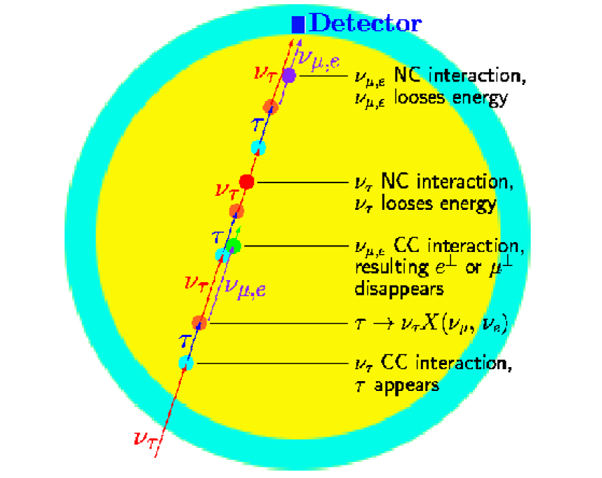
Figure 1: Schematic view of processes induced by high energy $\nu_{\tau}$’s when propagating through the Earth.

We have assumed the Earth composition made by standard rock ($A$=22, $Z$=11) of variable density with the Earth density profile published in [32]. Processes undergone by $\tau$-neutrinos during propagation through the Earth are shown schematically in Fig. 1.

2.1 Neutrino interactions

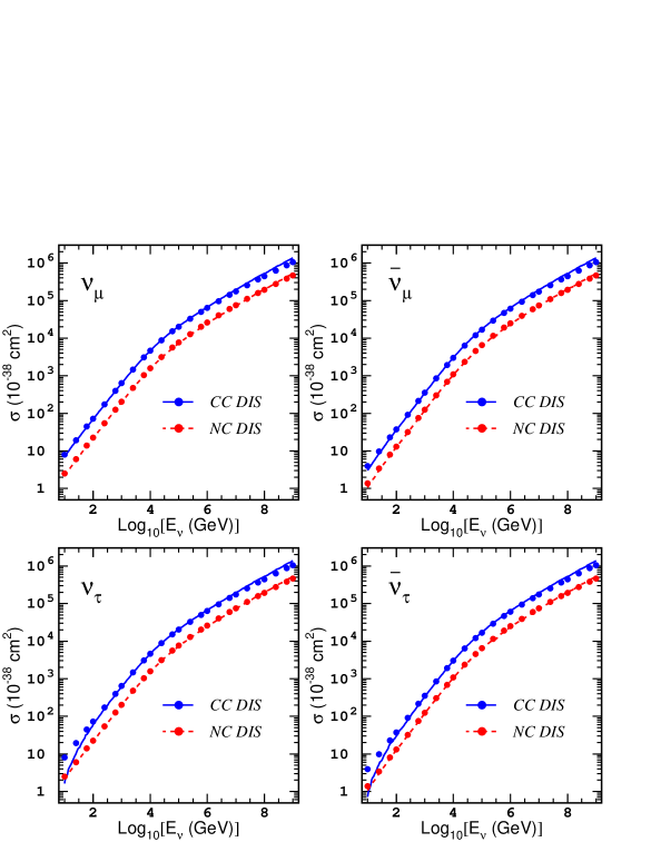
Figure 2: CC (solid lines) and NC (dashed lines) deep inelastic scattering cross-sections for $\nu_{\tau}$, $\bar{\nu}_{\tau}$, $\nu_{\mu}$, and $\bar{\nu}_{\mu}$ (cross-sections for electron (anti-)neutrinos practically coincide with ones for muon (anti-)neutrinos) for isoscalar medium with $Z/A$ = 0.5. Lines: cross-sections with structure functions CTEQ3-DIS (used in this work); markers: cross-sections with CTEQ4-DIS (from [42]).

To simulate $\nu\,N$ interactions we have used a generator developed by P. Lipari and F. Sartogo which is based on cross-sections described in [33]. It has been adapted for our use up to the high energy region we are interested in ($E_{\nu}>10^{5}$ GeV) adjusting the efficiency of the rejection technique method described in [34]. Both for NC and CC interactions we have accounted only for deep inelastic scattering since in the considered energy range other channels contribute negligibly. For what concerns deep inelastic scattering, the generator uses the electroweak standard formula for the inclusive differential cross-section and it is based on the LUND packages for hadronization [34, 35, 36]. Structure functions CTEQ3-DIS [37] taken from PDFLIB [38] suited for the high energy regime have been used . More recent versions of CTEQ PDFs [39, 40, 41] produce differences on cross-sections at the level of up to 25% at $10^{9}$ GeV (see Fig. 2).

2.2 Tau-lepton energy losses

The MUM package (version 1.5) has been used to simulate $\tau$-lepton propagation through matter. Comparing to [43] (where the first version of the package originally developed for the muon propagation was described) the package has been extended to treat $\tau$-leptons, accounting for their short life time and large probability to decay in flight. Besides, the newest corrections to photonuclear cross-section have been introduced. Formulas for cross-sections for $e^{+}e^{-}$-pair production, bremsstrahlung, knock-on electron production and stopping formula for ionization implemented in MUM 1.5 can be found in [43] (Appendix A)  where they are given according to [50, 51, 52, 53, 54, 55, 56, 57, 58, 59, 60].

Main improvements in MUM 1.5 concern photonuclear interaction of leptons with nucleons, in which virtual photons are exchanged. We are interested in the diffractive region of the kinematic variable space ($q^{2}<0$, transferred energy $\nu$ large, $x_{Bj}\sim q^{2}/2\nu$ small). The photonuclear interaction has been treated as the absorption of the virtual photon by the nucleon and, using the optical theorem, it has been connected with the Compton scattering of a virtual photon, $\gamma^{*}+N\to\gamma^{*}+N$. The Compton scattering in the diffractive region has been described by the vacuum exchange which, in turn, is modeled in QCD by the exchange of two or more gluons in a color singlet state. This is possible because, in the laboratory system, the interaction region has a large longitudinal size, and the photon develops an internal structure due to its coupling with quark fields. In the diffractive region, $\gamma^{*}N$-scattering dominates the Compton amplitude, while the contribution to it due to the photon bare component is smaller.

It has been shown by HERA experiments [61, 62, 63, 64, 65, 66] that the picture of the usual soft diffraction, soft pomeron exchange, does not work well if the center-of-mass energy of $\gamma^{*}$ and the target nucleon $N$ is very large (i.e. if $q^{2}$ and $\nu$ are in the diffractive region). For a description of the data in the framework of the simplest Regge-pole model, one needs at least two pomerons: soft and hard ones. A two-component picture of the photonuclear interaction in the diffractive region arises very naturally due to inherent QCD properties (asymptotic freedom, confinement, color transparency) and is the common feature of some recent quantitative models [29, 44, 45]. Generally, the photonuclear cross-section integrated over $Q^{2}=-q^{2}$ is expressed through the electromagnetic structure functions of nuclei $\sigma_{L,T}$ by the formula

$$\frac{d\sigma^{pn}}{dv}=\frac{\alpha}{2\pi v}\int\limits^{\infty}_{Q^{2}_{min}}\frac{dQ^{2}}{Q^{2}}\{v^{2}\sigma_{T}(1-\frac{2m^{2}_{l}}{Q^{2}})+2(1-v)(\sigma_{T}+\sigma_{L})\},$$ (1)

where $Q^{2}_{min}\cong m^{2}_{l}v^{2}/(1-v)$, $v=\Delta E/E$ is the fraction of energy lost in the interaction by a lepton of energy $E$ with mass $m_{l}$ and $\alpha=$ 1/137 is the fine structure constant.

In the first version of the MUM code [43] only the soft part of this integral was accounted for according to Bezrukov-Bugaev (BB) parameterization that was developed in the frame of the generalized vector dominance model [30, 31]. In MUM 1.5 two main improvements have been done. Firstly, new terms have been included in the BB parameterization [29]. Since these produce negligible effects in the case of muon, they were not introduced in the original formula given in [30, 31]. Nevertheless, these terms are essential in case of $\tau$-lepton (due to its larger mass compared to muon: $m_{\mu}$=0.1057 GeV; $m_{\tau}$=1.777 GeV) and they increase total $\tau$-lepton energy losses by $\sim$20$\div$30% in UHE/EHE range. Secondly, the hard component of the photonuclear cross-section has been introduced using results obtained in [29]. This part is described by the phenomenological formula based on the color dipole model [46, 47]. The main element of the approach used in [29] is the total cross-section $\sigma(r_{\bot},s)$ for scattering of dipoles ($q\bar{q}$-pairs) of a given transverse size $r_{\bot}$ from a target proton at fixed center-of-mass energy squared $s$. The $r_{\bot}$-dependence of $\sigma(r_{\bot},s)$ is qualitatively predicted by perturbative QCD:

$$\sigma(r_{\bot},s)\sim r^{2}_{\bot}e^{-\frac{r_{\bot}}{r^{0}_{\bot}}}(r^{2}_{\bot}s)^{\lambda_{H}}.$$ (2)

In this formula $\lambda_{H}$ and $r^{0}_{\bot}$ are parameters determined from a comparison of the total photonuclear cross-section (or structure functions) with HERA data at small $x_{Bj}$. Such an expression for $\sigma(r_{\bot},s)$ was suggested in [48]. Besides, for a region of large $s$ (outside of the HERA region) the unitarization procedure is used in [29], which leads, asymptotically, to a logarithmic $s$-dependence of the dipole cross-section,

$$\sigma^{unit}(r_{\bot},s)\sim\lambda_{H}\ln s.$$ (3)

The hard part of the photonuclear cross-section is shown in Fig.4 and Fig.5 in [29] for muons and $\tau$’s, respectively. We have made a polynomial parameterization for this part that is given in Appendix A along with the complete formula for photonuclear cross-section used in this work.

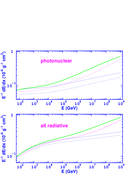
Figure 3: $\tau$-lepton energy losses in standard rock. Upper plot: energy losses due to photonuclear interaction. Lower plot: energy losses due to all radiative processes, including bremsstrahlung and direct $e^{+}e^{-}$-pair production computed according to [50, 51, 52, 53, 54, 55, 56]. In each plot: dashed line is for non corrected soft part [30, 31]; dash-dotted line for corrected soft part [29, 30, 31]; dotted line includes hard component of photonuclear cross-section according to [49]; solid line: includes hard component according to [29] (as it is treated in this work).

$\tau$-lepton energy losses in standard rock ($A$=22, $Z$=11) for photonuclear interaction and for the sum of all radiative processes are presented in Fig. 3. The importance of both corrections described above compared to the soft BB formula can be clearly seen. Results published in [49] for $\tau$-lepton energy losses including another calculation of the hard component of the photonuclear cross-section are shown for comparison, as well. The main difference between [29] and [49] is due to the fact that corrections to the BB formula (soft part) [30, 31] have not been introduced in [49]. The hard component of the photonuclear cross-section differs in [29] and [49], as well, since theoretical approaches applied in these two works are completely different.

2.3 Tau-lepton decay

To generate $\tau$-lepton decays we used the TAUOLA package [67] which was developed for SLC/LEP experiments where $\tau$-leptons are produced in $e^{+}e^{-}$ collisions: $e^{+}e^{-}\rightarrow Z\rightarrow\tau^{+}\tau^{-}$. TAUOLA generates decays of $\tau^{\pm}$’s of a given energy, taking into account all the effects of $\tau$ spin polarization. 22 decay modes are treated (sum to almost 100% of the total width) including modes that are responsible for $\nu_{e}$ and $\nu_{\mu}$ appearance:

$$\tau^{-}\rightarrow\,\,e^{-}\,\,\bar{\nu}_{e}\,\,\nu_{\tau}\,\,\,\,\,\,\,(\tau^{+}\rightarrow\,\,e^{+}\,\,\nu_{e}\,\,\bar{\nu}_{\tau})$$ (4)

$$\tau^{-}\rightarrow\,\,\mu^{-}\,\,\bar{\nu}_{\mu}\,\,\nu_{\tau}\,\,\,\,\,\,\,(\tau^{+}\rightarrow\,\,\mu^{+}\,\,\nu_{\mu}\,\,\bar{\nu}_{\tau})$$ (5)

In our simulation we tracked only neutrinos (of all flavors) resulting from $\tau$ decay, since ranges of charged leptons are negligibly small compared to the Earth dimensions. Decay lengths of $K$’s and $\pi$’s resulting from $\tau$ decay are much longer than their interaction lengths in the considered energy range, hence we did not simulate their decay neglecting secondary neutrinos .

3 Results on $\nu_{\tau}$ propagation through the Earth

In this section results on the simulation of propagation of $\nu_{\tau}$ and $\bar{\nu}_{\tau}$ monoenergetic beams through the Earth are presented where all processes shown in Fig. 1 have been accounted for.

3.1 Results on monoenergetic tau-neutrino beams

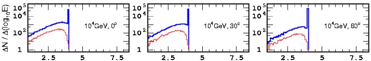
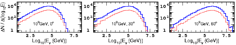
Figure 4: Monoenergetic $\nu_{\tau}$ beams incident on the Earth at nadir angles 0^∘ (left), 30^∘ (center), 60^∘ (right). Results after propagation through the Earth. Upper row: $E^{0}_{\nu}=$10 TeV, lower row: $E^{0}_{\nu}=$ 1 EeV. Upper spectra: $\nu_{\tau}$; lower spectra: secondary $\nu_{\mu}$ ($=\nu_{e}$).

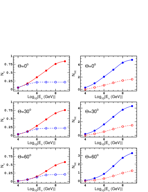
Figure 5: Left column: Mean number of secondary $\nu_{\mu}$’s ($=\nu_{e}$’s) per $\nu_{\tau}$ that are generated when a $\nu_{\tau}$ crosses the Earth undergoing regeneration processes vs $E_{\nu_{\tau}}$ (solid lines); mean number of secondary $\nu_{\mu}$’s ($=\nu_{e}$’s) that survive and come out from the Earth (dashed lines). Right column: mean number of CC (solid lines) and NC (dashed lines) interactions that occurs in the chain $\nu_{\tau}\rightarrow\tau\rightarrow\nu_{\tau}\cdots$ when a $\tau$-neutrino crosses the Earth vs its energy. Results for $\nu_{\tau}$ and $\bar{\nu}_{\tau}$ are identical.

The outgoing spectra of initially monoenergetic $\nu_{\tau}$’s after propagation through the Earth for three nadir angles of incidence on the Earth are shown in Fig. 4 for two neutrino energies: 10 TeV and 1 EeV. Moreover, the outgoing spectra of secondary $\nu_{\mu}$’s and $\nu_{e}$’s that are produced in decays of $\tau$-leptons generated in $\nu_{\tau}$ CC interactions are presented. Results for $\nu_{\tau}$ and $\bar{\nu}_{\tau}$ beams are identical. At $E_{\nu_{\tau}}=$10⁴ GeV neutrino cross-sections are small and most of $\tau$-neutrinos cross the Earth without interacting keeping their initial energy (see the peaks in the upper panels in Fig. 4). The fraction of such neutrinos is lower at the nadir direction ($\theta=$ 0^∘) since the amount of matter crossed is maximum. This fraction increases with nadir angle. At $E_{\nu_{\tau}}=10^{9}$ GeV all $\tau$-neutrinos undergo at least one interaction and the peak at initial energy disappears since neutrinos loose energy both in NC interactions and in regeneration chain. The fraction of secondary $\nu_{e}$’s and $\nu_{\mu}$’s produced by the incoming $\nu_{\tau}$ is 5% at $E_{\nu_{\tau}}=$10⁴ GeV and 22% at $E_{\nu_{\tau}}=$10⁹ GeV for the nadir direction . These numbers are in good agreement with results published in [15].

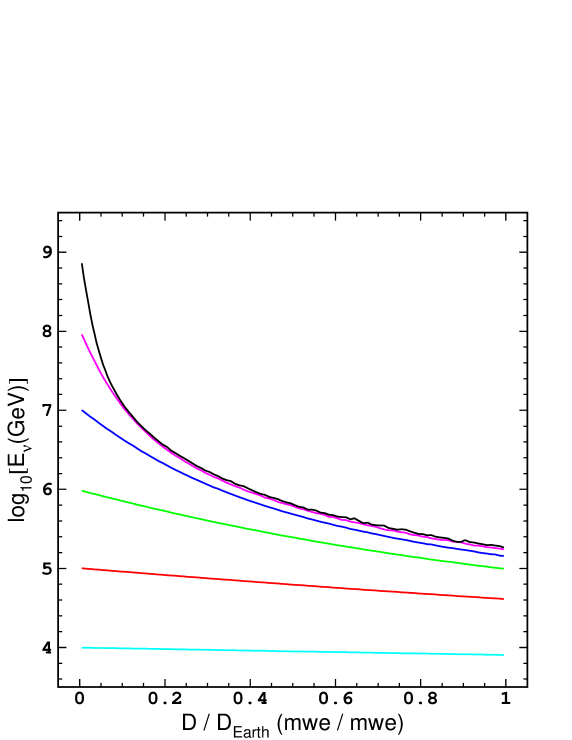
Figure 6: Mean energy degradation for $\nu_{\tau}$ with initial energies (from bottom to top): 10⁴ GeV, 10⁵ GeV, 10⁶ GeV, 10⁷ GeV, 10⁸ GeV, 10⁹ GeV when penetrating the Earth at nadir angle 0^o vs fraction of Earth diameter crossed.

The fraction of secondary neutrinos that accompany $\tau$-neutrinos emerging from the Earth increases with initial $\tau$-neutrino energy but saturates at the level of 0.22 at some critical energy which depends upon nadir angle (Fig. 5, left column). These results are also in a good agreement with [15]. The CC cross-section increases with energy and, consequently, the number of secondaries generated along $\tau$-neutrino path increases also. Nevertheless, this growth is moderated by absorption of secondary $\nu_{\mu}$’s and $\nu_{e}$’s which, in contrast to $\nu_{\tau}$’s, do not regenerate. In the right column in Fig. 5 the mean number of NC and CC interactions occurring to a primary $\nu_{\tau}$ ($\bar{\nu}_{\tau}$) when it travels through the Earth is shown The number of CC interactions corresponds to the number of regeneration steps. This number grows both with $\tau$-neutrino energy and with amount of matter crossed, which is maximum at the nadir.

Fig. 6 shows $\tau$-neutrino energy losses due to regeneration process and NC interactions when crossing the Earth.

3.2 Results for some astrophysical diffuse $\nu$ spectra

We performed MC simulations for two spectra of cosmological neutrinos: the spectrum predicted by Protheroe [27] for an optically thick proton blazar model and an upper bound (not a source model) on diffuse $\nu$ spectrum for optically thick sources [28] (MPR bound)  (see Fig. 7).

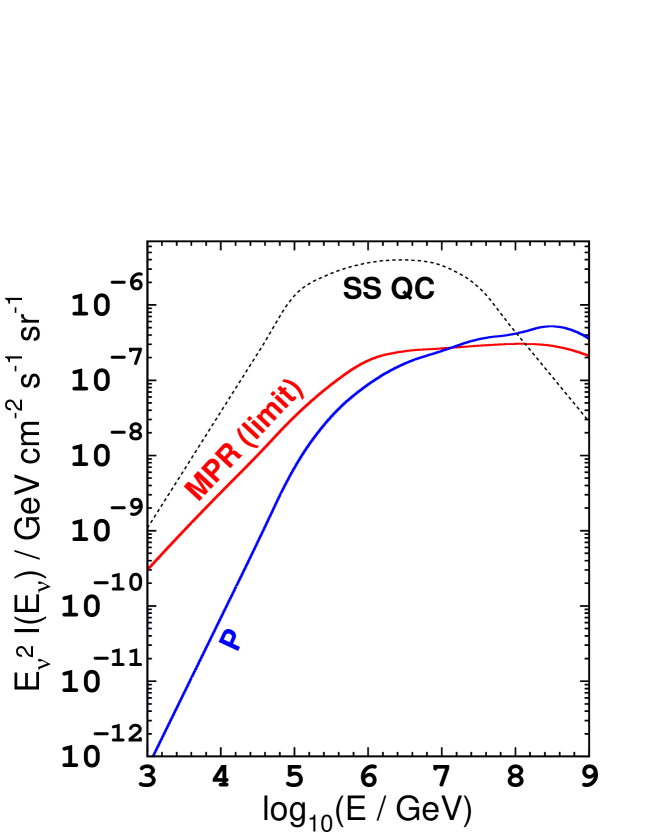
Figure 7: Protheroe diffuse neutrino spectrum [27], MPR limit on diffuse neutrino spectrum [28] and ’Quasar background flux prediction’ (SS QC) [68].

We have considered neutrinos of all flavors in the incoming flux including $\nu_{e}$’s and $\nu_{\mu}$’s produced in sources and $\nu_{\tau}$’s that appear on the way to the Earth due to $\nu_{\mu}\leftrightarrow\nu_{\tau}$ oscillations. Neutrinos and anti-neutrinos of all flavors have been assumed to be present in the proportion $\phi_{\nu}\!:\!\phi_{\bar{\nu}}\!=\!1\!:\!1$ in astrophysical neutrino fluxes. The background of $\nu_{\mu,e}$ atmospheric neutrinos from pion and kaon decays (conventional neutrinos), as well as the contribution of prompt $\nu$’s from charmed mesons (calculated in the Recombination Quark-Parton Model frame) was simulated using spectra taken from [72].

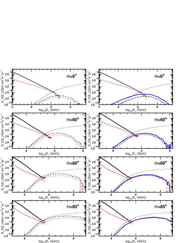
Figure 8: Spectra of cosmological $\nu$’s sampled according to Protheroe spectrum ([27]) incident on the Earth with 4 different nadir angles and after propagation through it. Left column: no oscillations, $\phi_{\nu_{e}}\!:\!\phi_{\nu_{\mu}}\!:\!\phi_{\nu_{\tau}}=1\!:\!2\!:\!0$, right column: oscillations with maximal mixing, $\phi_{\nu_{e}}\!:\!\phi_{\nu_{\mu}}\!:\!\phi_{\nu_{\tau}}=1\!:\!1\!:\!1$. Thin solid lines: total incoming flux of astrophysical $\nu$’s; thick solid (right panels), dashed and dash-dotted lines (overlapping in right panels): out-coming $\nu_{\tau}+\bar{\nu}_{\tau}$, $\nu_{\mu}+\bar{\nu}_{\mu}$, $\nu_{e}+\bar{\nu}_{e}$ after propagation through the Earth, respectively. $\nu_{\mu,e}$ spectra include secondary neutrinos produced by $\nu_{\tau}$’s. In the left part of each panel atmospheric neutrino spectra (conventional$+$prompt [72]) after propagation through the Earth are shown, upper thick markers: $\nu_{\mu}+\bar{\nu}_{\mu}$, lower thin markers: $\nu_{e}+\bar{\nu}_{e}$. Atmospheric neutrino spectra are given up to $\approx$300 TeV where cosmological neutrino fluxes start to dominate since the simulation statistics at higher energies is very poor due to the steepness of spectra.

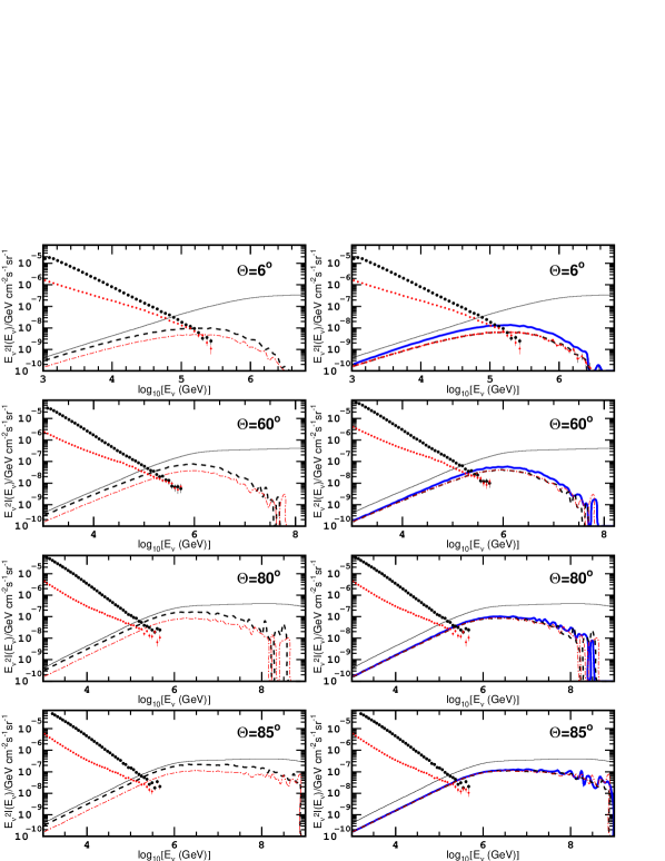
Figure 9: The same as in Fig. 8 but astrophysical neutrinos are generated according to MPR upper limit on diffuse neutrino flux [28].

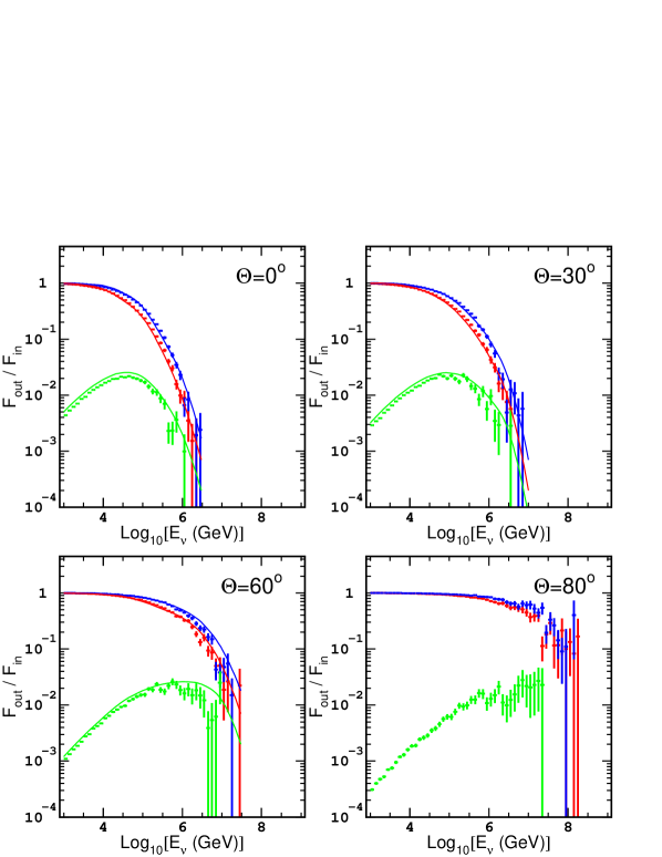
Figure 10: The ratio of $\nu_{\tau}+\bar{\nu}_{\tau}$ (upper curves), $\nu_{\mu}+\bar{\nu}_{\mu}$ (middle curves) fluxes after propagation through the Earth and of secondary $\nu_{\mu}+\bar{\nu}_{\mu}$ ($=\nu_{e}+\bar{\nu}_{e}$) (lower curves) over incident flux $\propto E^{-2}$ for four nadir angles. Markers: this work, lines: results published in [16] for nadir angles $\theta$ =0^∘, $\theta$ =30^∘ and $\theta$ =60^∘ (data for $\theta$ =80^∘ are absent in [16]).

Results for Protheroe and MPR spectra for astrophysical neutrinos incident on the Earth with 4 different nadir angles and transformed after propagation through the Earth are shown in Fig. 8 and Fig. 9. $\tau$-neutrino fluxes exceed $\nu_{\mu,e}$ ones remarkably up to nadir angles $\theta\sim 60^{o}$ since $\nu_{\tau}$’s are not absorbed by the Earth in contrast to $\nu_{\mu,e}$’s. But their spectra are shifted to lower energies with respect to initial spectra due to energy degradation in regeneration processes. For all $\theta$, the outgoing flux of astrophysical neutrinos exceeds the background of atmospheric neutrinos at $E_{\nu}\gtrsim 10^{5}$ GeV. This cross-over determines the energy threshold for detection of diffuse neutrino fluxes in UNTs. Results for Protheroe spectrum are in a qualitative agreement with ones published in [13] (see Fig. 8 and Fig. 9 there) where different models for neutrino interactions and $\tau$-lepton energy losses were used. The fractions of secondary $\nu_{\mu,e}$’s produced in regeneration chains with respect to the total $\nu_{\mu,e}$ flux emerging after propagation through the Earth (made of of primary $\nu_{\mu,e}$’s $+$ secondaries) are 0.57, 0.18, 0.06, 0.02 (spectrum [27]) and 0.18, 0.06, 0.02, 0.01 (spectrum [28]) for nadir angles $\theta=$6^o, 60^o, 80^o, and 85^o, respectively. These numbers are larger than corresponding fractions for power-law spectra $\phi_{\nu}\propto E_{\nu}^{-1}$ and $\phi_{\nu}\propto E_{\nu}^{-2}$ reported in [16] . On the other hand, the comparison of the results on attenuated neutrino fluxes obtained by our algorithm with the ones obtained in [16] for power-law spectra shows a reasonable agreement (Fig. 10). Hence, we can conclude that larger fractions of secondaries result from the fact that MPR and Protheroe spectra are harder compared to ones considered in [16].

4 Tau leptons: detection signatures

4.1 Tau lepton identification through energy loss properties

At energies larger than $E_{\tau}\approx$ 2$\cdot$10⁶ GeV $\tau$-lepton ranges become comparable to the typical linear dimensions of operating and proposed UNTs (see Fig. 11) and $\tau$ tracks can be reconstructed. As a first guess, one could try to distinguish a $\tau$-lepton track from a muon one by means of differences in energy losses. The larger $\tau$ mass affects bremsstrahlung, $e^{+}e^{-}$-pair production and photonuclear processes differently respect to muons. As a result, $e^{+}e^{-}$-pair production dominates muon energy losses up to $E_{\mu}\approx$ 10⁸ GeV while $\tau$-lepton photonuclear interaction plays the main role above $E_{\tau}\approx$ 10⁵ GeV (see Fig. 12) compared to other radiative processes. Hence, since probabilities of shower production for muons and $\tau$-leptons at a given energy are different, one could hope to select $\tau$-lepton events studying the distribution of showers produced in photonuclear or electromagnetic interactions along tracks even if the detector resolution is not so good to discriminate hadronic and electromagnetic showers.

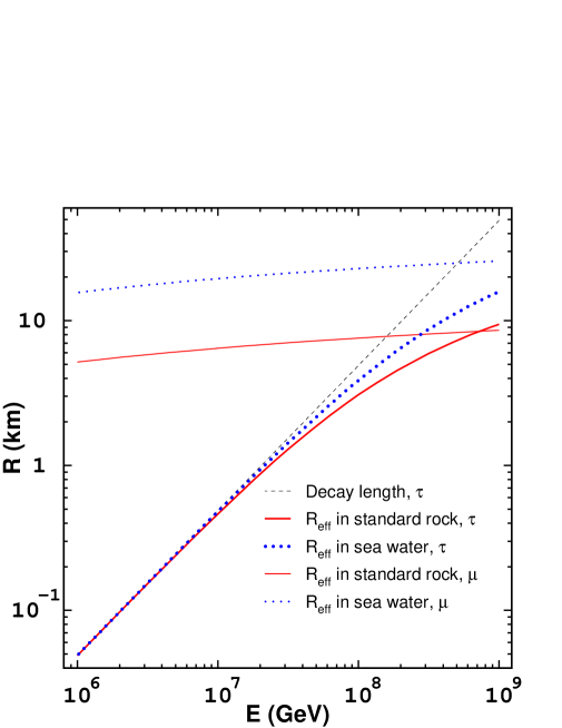
Figure 11: Mean ranges for muons and $\tau$-leptons in standard rock and sea water.

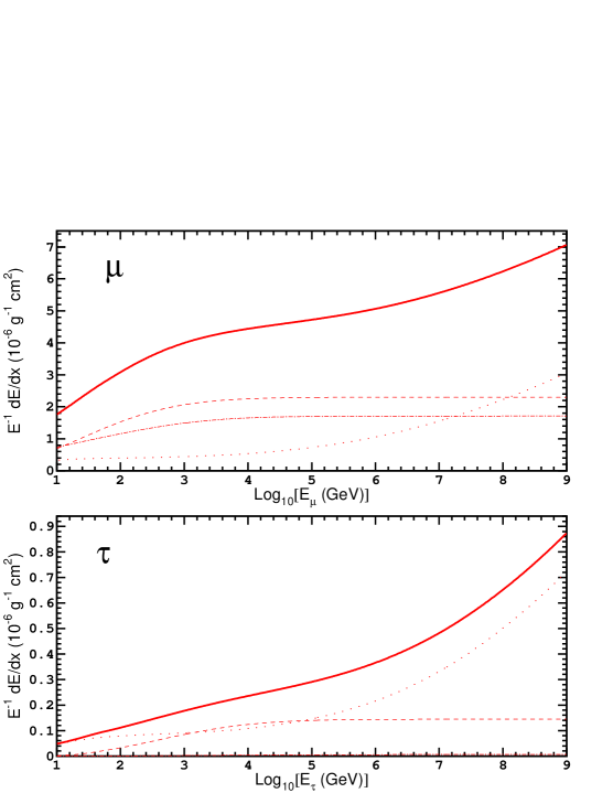
Figure 12: Muon (upper plot) and $\tau$-lepton (lower plot) energy losses in standard rock due to bremsstrahlung (dash-dotted lines), direct $e^{+}e^{-}$-pair production (dashed lines), photonuclear interaction (dotted lines). Thick solid lines stand for total radiative energy losses. Bremsstrahlung for $\tau$-lepton is strongly suppressed due to $m^{-2}$ factor, therefore the bremsstrahlung curve almost coincides with the $x$-axis.

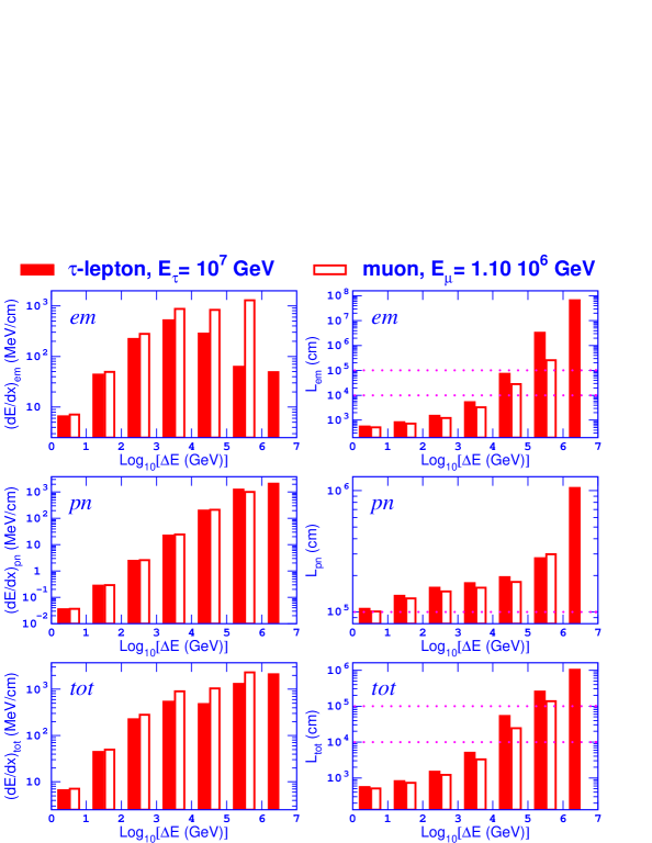
Figure 13: Left column: energy losses in sea water due to electromagnetic interactions (upper panel), photonuclear interactions (middle panel) and all interactions (lower panel) for energy transferred to secondaries belonging to different ranges ($10^{0}GeV\leq\Delta E\leq 10^{1}GeV$, $10^{1}GeV\leq\Delta E\leq 10^{2}GeV$, …, $10^{6}GeV\leq\Delta E\leq 10^{7}GeV$). Filled boxes correspond to a $\tau$-lepton with $E_{\tau}$ = 10⁷ GeV, empty ones to a muon with energy $E_{\mu}$ = $1.1\,10^{6}$ GeV. Right column: Mean interaction length of muon/$\tau$-lepton in sea water for different ranges of energy transfered to secondaries. The horizontal lines indicate 100 m and 1 km which are the typical linear sizes of existing and planned UNTs.

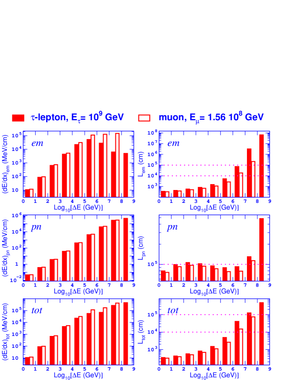
Figure 14: The same as in Fig. 13 for a 10⁹ GeV $\tau$-lepton and a $1.56\cdot 10^{8}$ GeV muon.

Nevertheless, the results of the calculation that we have performed for $\tau$-leptons with energies in the range 10⁶ GeV$\leq E_{\tau}\leq$10⁹ GeV indicate that such a method works badly because the largest differences between shapes of $\tau$-lepton and muon cross-sections lies in a range of relatively large $v=\Delta E/E$, where interaction lengths exceed the detector size. The numerical data on $\tau$-leptons of energies 10⁷ GeV and 10⁹ GeV and muons of lower energies (1.10$\cdot$10⁶ and 1.56$\cdot$10⁸, respectively) are presented in Fig. 13 and Fig. 14, which show values of energy losses and radiation lengths for different ranges of energy transfered to secondaries ($10^{0}GeV\leq\Delta E\leq 10^{1}GeV$, $10^{1}GeV\leq\Delta E\leq 10^{2}GeV$, …, $10^{6}GeV\leq\Delta E\leq 10^{7}GeV$). Muon energies were chosen so that total muon energy losses are equal to total energy losses of considered $\tau$-leptons. Data on electromagnetic processes (bremsstrahlung $+$ $e^{+}e^{-}$-pair production), photonuclear interaction and all interactions are presented separately. One can see that ’partial’ energy losses and radiation lengths of $\tau$-leptons and muons of lower energies differ remarkably only for large transferred energies when radiation length exceeds 100 - 1000 m, typical linear dimensions of existing and planned detectors. Thus, there are too few high energy showers inside the detector sensitive volume to provide enough statistics to distinguish $\tau$-lepton and muon tracks. Even in the hypothesis that the detector capability is so good to distinguish electromagnetic showers from hadronic ones, it is very difficult and, most probably, impossible to distinguish a $\tau$-lepton track of a certain energy with respect to a muon track of $\sim$6$\div$11 times lower energy. This difficulty also concerns 1 km³-scale UNTs. Of course, the observation of a very high energy shower with reconstructed energy so large to be inconsistent with the energy reconstructed using the rest of the track could be an indication in favor of a $\tau$-lepton. Nevertheless, the probability of such a shower occurrence is too small that this cannot be considered a standard reliable method.

4.2 Topological signatures

As a matter of fact, signatures such as ’double bang’ (DB) or ’lollipop’ events proposed in [21] seem to be smoking guns to recognize $\tau$-lepton events in UNTs. DB event features are an hadronic cascade at the $\nu\,N$ CC interaction vertex and an hadronic or electromagnetic cascade corresponding to $\tau$-lepton decay. The $\tau$-lepton track connects both cascades . A lollipop event consists of a partially contained $\tau$-lepton track with the first cascade at the $\nu$ interaction vertex outside of the UNT sensitive volume and with the second cascade produced by $\tau$-lepton decay contained in the volume. On the other hand, the inverse pattern with only the first cascade visible can not be distinguished from $\nu_{\mu}\,N\to\mu\,N$ interaction followed by the muon track. Both DB and lollipop signatures provide a clear and background-free evidence of $\nu_{\tau}$ detection. As a matter of fact, for $\tau$ decaying into electronic and hadronic channels there is no muon track following the second cascade. Besides, DB events do not contain an in-coming track before the first cascade. In principle, an up-going muon generated in a $\nu_{\mu}$ CC interaction could mimic such a signature if it would produce a shower that takes all the muon energy inside the instrumented volume. But the probability to have such an event for a muon track segment of the order of 1 km is less than 5$\cdot$10^-4 in water for energies larger than 1 PeV. This value corresponds to the probability that a muon looses more than 99% of its energy in one interaction. This number can be considered as an upper limit on the signal to noise ratio, where the signal are DB/lollipop events and the noise are up-going $\nu$-induced muons. In fact, astrophysical $\nu_{\mu}$ fluxes are lower or at most equal to expected astrophysical $\nu_{\tau}$ ones after propagation in the Earth and atmospheric neutrino fluxes are even lower above 1 PeV (see Fig. 8 and Fig. 9). Another background source could be due to atmospheric muons that are dominated by prompt muons in the considered energy range. DB events cannot be reproduced since in any case the muon track before the first cascade would be visible. Nevertheless, a muon can mimic a lollipop event if it enters the detector instrumented volume and undergoes an interaction with such a large energy transfer that the muon stops after shower production. We estimate a rate of $\sim 50$ km^-3 yr^-1 considering the probability upper limit of $5\cdot 10^{-4}$ (corresponding to more than 99% muon energy loss) and the prompt muon fluxes published in [73, 74]. However, this is an upper limit since it is not possible to compute exactly the probability that a muon looses 100% of its energy since cross section parameterizations close to $v=\Delta E/E=1$ do not describe perfectly well the real cross sections. Of course more quantitative conclusions on possible backgrounds are needed that should be based on detailed simulations including detector response and reconstruction algorithms. At least qualitatively, DB and lollipop events are potentially “background free”, as it has been stated in the paper that proposed the existence of these topologies [21].

In 17% of the cases, that is for the $\tau$ decay channel into a muon (see eq. 5), the second cascade is absent. In this case the $\tau$-lepton track is followed by a muon track without any shower. This topology seems to be not-recognizable as a $\tau$-lepton signature in a UNT, although the amount of light produced by showers along the $\tau$ track (hereafter ’brightness’) differs essentially from that along a muon track of the same energy. As an example, let us consider a $\tau$-lepton of energy $E_{\tau}$= 10⁷ GeV that decays into a muon. For a simple estimation, we assume that the muon takes 1/3 of the $\tau$ energy, thus $E_{\mu}\approx$ 3.3$\cdot$10⁶ GeV. From results in Sec. 4.1 (see Fig. 13) we know that the brightness of a 10⁷ GeV $\tau$ track is similar to that of a $\mu$ track with $E_{\mu}=1.1\cdot 10^{6}$ GeV. After $\tau$-lepton decay, the track brightness increases by about a factor of $\approx$3.3$\cdot$10⁶ GeV$/$1.1$\cdot$10⁶ GeV$=$3. This factor depends on $\tau$-lepton energy and in the range 10⁶ GeV $\leq E_{\tau}\leq$ 10⁹ GeV it varies between 2 and 4. To recognize such a signature detector energy reconstruction should be remarkably better than this factor, which is not always the case for neutrino telescopes (see for instance Fig. 4 from [75]). Thus, when computing DB or/and lollipop event rates in a UNT, results must be reduced by a factor $B_{-\mu}$= 0.83 to exclude the non-muonic branching ratio in $\tau$-lepton decay.

Estimates of DB rates in km³ UNTs have already been presented in [22] for down-going $\nu_{\tau}$’s, while events from the lower hemisphere were not considered. Calculations of up-going $\nu_{\tau}$ propagation were done in [14]. Authors give a qualitative conclusion that though UHE/EHE $\nu_{\tau}$’s are not absorbed by the Earth, their energies decrease; hence the expected amount of $\tau$ events in the DB energy range is low. Calculations in [24] performed for a neutrino flux $E^{2}_{\nu_{\mu}}\,dN_{\nu_{\mu}}\,/\,dE_{\nu_{\mu}}=$ 10^-7 GeV cm^-2 s^-1 assuming $\nu$ oscillations but without accounting for neutrino absorption in the Earth result in a rate of $\approx$0.5 yr^-1 both for DB and lollipop events in an IceCube-like km³ detector [4]. The measurement of the ratio between muon and shower events that may be an indirect signature of $\nu_{\tau}$ appearance was proposed in [14, 24] as an alternative indirect way to detect $\tau$-neutrinos. Here we present results of a calculation of the DB rate for both the upper and lower hemispheres in a km³ scale UNTs using results reported in Sec. 3 for the spectra in [27, 28] that were not considered in [14, 22, 24]. The rate of totally contained DB events in a UNT is given by:

$$n_{DB}=2\pi\,\rho\,N_{A}\,B_{-\mu}\!\!\!\int_{-1}^{0(1)}\!\!\int^{\infty}_{E_{min}}\!\!V_{eff}(E_{\nu_{\tau}},\theta)\,I(E_{\nu_{\tau}},\theta)\,\sigma^{CC}(E_{\nu_{\tau}})\,dE_{\nu_{\tau}}d(\cos\theta)$$ (6)

Here $N_{A}$ is the Avogadro number, $\rho$ is the medium density (we use $\rho=$ 1 g cm^-3 which is close to sea water/ice density), $I(E_{\nu_{\tau}},\theta)$ is the differential $\nu_{\tau}$ flux. The Earth shadowing effect is accounted for in the case of the lower hemisphere (for which the upper limit of the integral is 0, while $\cos\theta=1$ is used to compute the number of events for the whole sphere). The effective volume is:

$$V_{eff}=S_{p}(\theta)\,(L-R_{\tau}(E_{\nu_{\tau}}))\,,$$ (7)

where $S_{p}$ is the projected area for tracks generated isotropically in azimuth for a fixed $\theta$ direction of the incident neutrino on a parallelepiped. The parallelepiped has the dimensions of an IceCube-like detector [4] ($1\!\times\!1\!\times\!1$ km³) or a NEMO-like one [5] ($1.4\!\times\!1.4\!\times\!0.6$ km³). In eq. 7, $L$ is the geometrical distance between entry and exit point from the parallelepiped, $R_{\tau}$ is the $\tau$-lepton range, $\sigma^{CC}$ is total CC $\nu$ cross-section. $E_{min}\!=\!2\cdot 10^{6}$ GeV corresponds to a $\tau$-lepton range of $R^{min}_{\tau}\!=\!70$ m.

Table 1: Number of DB events in km³ detector per year.

Spectrum	IceCube-like ($N_{-2\pi}\,/\,N_{2\pi}\,/\,N_{4\pi}$)	NEMO-like ($N_{-2\pi}\,/\,N_{2\pi}\,/\,N_{4\pi}$)
$Protheroe$	$0.6\,\,\,\,/\,\,\,\,1.3\,\,\,\,/\,\,\,\,1.9$	$0.8\,\,\,\,/\,\,\,\,1.7\,\,\,\,/\,\,\,\,2.5$
$MPR$	$0.8\,\,\,\,/\,\,\,\,1.9\,\,\,\,/\,\,\,\,2.7$	$1.2\,\,\,\,/\,\,\,\,2.6\,\,\,\,/\,\,\,\,3.8$

Table 1 shows DB rates for the lower, upper and for both hemispheres. Values for upper hemisphere are 3$\div$6 times lower compared to [22] since more optimistic predictions for diffuse neutrino fluxes [68] are used there. At the same time, our figures for DB rates in IceCube-like UNT are 4$\div$5 higher compared to results reported in [24]. There are at least four factors that contribute to this difference:

• different $\nu$ flux models are used;

• minimum $\tau$ range is $R^{min}_{\tau}\!=\!70$ m in our calculations while in [24] it is equal to $R^{min}_{\tau}\!=\!200\div 400$ m. Such a large minimum range was chosen according to the qualitative requirement to reconstruct the $\tau$-lepton track connecting the two cascades. This difference accounts for a factor of $\sim$4 in the case of an $E^{-2}$ $\nu$ flux between $10^{6}$ and $10^{7}$ GeV. Since horizontal photomultiplier spacing in IceCube detector is $\sim$125 m, but the vertical spacing is 17 m [4], we believe that this requirement could be too restrictive. The proper choice of the minimum range should indeed be done quantitatively using a full simulation of the detector including reconstruction procedures;

• for the lower hemisphere we accounted for $\tau$-neutrino energy losses in the Earth. This losses can be such that events do not fall anymore above the DB ‘energy threshold’ (that figures for lower hemisphere in Table 1 are about a factor of $\approx$2 lower compared to the upper hemisphere ones). These losses were not accounted for in [24];

• in contrast to [24] we reduce all figures for rates by a factor $B_{-\mu}$= 0.83 to exclude the muonic mode of $\tau$-lepton decay.

5 Conclusions

Considering the AGN diffuse neutrino flux models in [27] and the upper limit on optically thick $\nu$ sources in [28] we have found that in a km³ UNT one can expect 2$\div$4 DB events yr^-1 . This result depends on the assumed neutrino spectrum and on the minimum $\tau$-lepton range that can be reconstructed in the detector, hence on its geometry and reconstruction algorithms. Hence, these values should be considered as indicative, while full simulations for specific neutrino telescopes should be performed. Moreover, we have investigated the possibility of identification of $\tau$-lepton from muons by studying the distribution of showers produced by electromagnetic and photonuclear interactions along the track. This seems to be very difficult. Detection of DB or lollipop events are the cleanest signatures even though rates seem to be quite small. An alternative indirect way to identify $\tau$’s consists in measuring the ratio between shower and track events. In any case, simulations of $\tau$-neutrino propagation through the Earth should be performed including regeneration processes and $\tau$-lepton energy losses. For this, in particular, one needs to account for corrections to the soft part of the photonuclear interaction which increases the total $\tau$-lepton energy losses by $\approx$20$\div$30% in UHE/EHE range.

Appendix A Appendix: photonuclear cross-section

The differential cross-section for photonuclear interaction used in this work has been published in [29]. It is rewritten below in the form adopted in [43] (Appendix A). In the formula the following values are used: $\alpha$ = 7.297353$\times$10^-3 – fine structure constant; $A\equiv$ atomic weight; $m_{l}=m_{\mu}=$ 0.1057 GeV for muon and $m_{l}=m_{\tau}=$ 1.777 GeV for $\tau$-lepton; $m_{N}\equiv$ nucleon mass; $\pi$ = 3.141593.

Table 2: Coefficients $a_{k}$ for $\frac{d\sigma^{pn}_{hard}}{dv}=\frac{1}{v}\sum^{7}_{k=0}\,a_{k}\log_{10}^{k}v$ in the formula for photonuclear cross-section. The upper figures stand for muons, lower ones does for $\tau$-leptons.

E ($GeV$)	$a_{0}$	$a_{1}$	$a_{2}$	$a_{3}$
$10^{3}$	7.174409$\cdot$10-4	-0.2436045	-0.2942209	-0.1658391
	-1.269205$\cdot$10-4	-0.01563032	0.04693954	0.05338546
$10^{4}$	1.7132$\cdot$10-3	-0.5756682	-0.68615	-0.3825223
	-2.843877$\cdot$10-4	-0.03589573	0.1162945	0.130975
$10^{5}$	4.082304$\cdot$10-3	-1.553973	-2.004218	-1.207777
	-5.761546$\cdot$10-4	-0.07768545	0.3064255	0.3410341
$10^{6}$	8.628455$\cdot$10-3	-3.251305	-3.999623	-2.33175
	-1.195445$\cdot$10-3	-0.157375	0.7041273	0.7529364
$10^{7}$	0.01244159	-5.976818	-6.855045	-3.88775
	-1.317386$\cdot$10-3	-0.2720009	1.440518	1.425927
$10^{8}$	0.02204591	-9.495636	-10.05705	-5.636636
	-9.689228$\cdot$10-15	-0.4186136	2.533355	2.284968
$10^{9}$	0.03228755	-13.92918	-14.37232	-8.418409
	-6.4595$\cdot$10-15	-0.8045046	3.217832	2.5487
E ($GeV$)	$a_{4}$	$a_{5}$	$a_{6}$	$a_{7}$
$10^{3}$	-0.05227727	-9.328318$\cdot$10-3	-8.751909$\cdot$10-4	-3.343145$\cdot$10-5
	0.02240132	4.658909$\cdot$10-3	4.822364$\cdot$10-4	1.9837$\cdot$10-5
$10^{4}$	-0.1196482	-0.02124577	-1.987841$\cdot$10-3	-7.584046$\cdot$10-5
	0.05496	0.01146659	1.193018$\cdot$10-3	4.940182$\cdot$10-5
$10^{5}$	-0.4033373	-0.07555636	-7.399682$\cdot$10-3	-2.943396$\cdot$10-4
	0.144945	0.03090286	3.302773$\cdot$10-3	1.409573$\cdot$10-4
$10^{6}$	-0.7614046	-0.1402496	-0.01354059	-5.3155$\cdot$10-4
	0.3119032	0.06514455	6.843364$\cdot$10-3	2.877909$\cdot$10-4
$10^{7}$	-1.270677	-0.2370768	-0.02325118	-9.265136$\cdot$10-4
	0.5576727	0.1109868	0.011191	4.544877$\cdot$10-4
$10^{8}$	-1.883845	-0.3614146	-0.03629659	-1.473118$\cdot$10-3
	0.8360727	0.1589677	0.015614	6.280818$\cdot$10-4
$10^{9}$	-2.948277	-0.5819409	-0.059275	-2.419946$\cdot$10-3
	0.8085682	0.1344223	0.01173827	4.281932$\cdot$10-4

$$\begin{array}[]{l}\frac{d\sigma^{pn}}{dv}=\frac{\alpha}{8\pi}A\sigma_{\gamma N}\,v\left\{\left(H(v)+\frac{2m_{l}^{2}}{m_{2}^{2}}\right)\ln\left(1+\frac{m_{2}^{2}}{t}\right)\right.\\[14.22636pt] \qquad-\left.\frac{2m_{l}^{2}}{t}\left[1-\frac{0.25m_{2}^{2}}{t}\ln\left(1+\frac{t}{m_{2}^{2}}\right)\right]+G(z)\left[H(v)\left(\ln\left(1+\frac{m_{1}^{2}}{t}\right)-\frac{m_{1}^{2}}{m_{1}^{2}+t}\right)\right.\right.\\[14.22636pt] \qquad+\left.\left.\frac{4m^{2}_{l}}{m^{2}_{1}}\ln\left(1+\frac{m^{2}_{1}}{t}\right)-\frac{2m_{l}^{2}}{t}\left(1-\frac{0.25m_{1}^{2}-t}{m_{1}^{2}+t}\right)\right]\right\}+A\frac{d\sigma^{pn}_{hard}}{dv},\end{array}$$

$$H(v)=1-\frac{2}{v}+\frac{2}{v^{2}},\qquad$$

$$G(z) = \frac{9}{z}\left[\frac{1}{2}+\frac{(1+z)e^{-z}-1}{z^{2}}\right]\qquad(Z\neq 1),$$

$$G(z) = 3\qquad(Z=1),$$

$$z=0.00282A^{1/3}\sigma_{\gamma N},\quad t=\frac{m_{l}^{2}v^{2}}{1-v},\quad m_{1}^{2}=0.54\;{\rm GeV}^{2},\quad m_{2}^{2}=1.80\;{\rm GeV}^{2}$$

with total cross-section for absorption of a real photon of energy $\nu=s/2m_{N}=vE$ by a nucleon, $\sigma_{\gamma N}$, parameterized according to [30, 31]

$$\sigma_{\gamma N}=[114.3+1.647\ln^{2}(0.0213\,\nu)]\,\mu b$$

and hard part of cross-section described by polynomial parameterization

$$\frac{d\sigma^{pn}_{hard}}{dv}=\frac{1}{v}\sum^{7}_{k=0}\,a_{k}\log_{10}^{k}v$$

(coefficients $a_{k}$ are given in Table 2). Parameterization for $\frac{d\sigma^{pn}_{hard}}{dv}$ is valid in the range $10^{-6}\leq v\leq 1$, $10^{3}\leq E\leq 10^{9}$ $GeV$, in MUM 1.5 $\frac{d\sigma^{n}_{hard}}{dv}$ is assigned to 0 for $E=$ 10² $GeV$ and $v=10^{-7}$, values between $v=10^{-7}$ and $v=10^{-6}$, as well as between $E=$ 10² GeV and $E=$ 10³ GeV are computed by interpolation. Values for energies between ones that are given in the Table 2 are computed by interpolation, as well.

References

- [1] AMANDA Collaboration: P. Desiati et al., astro-ph/0306536; see URL http://amanda.uci.edu/.
- [2] ANTARES Collaboration: E. Aslanides et al., astro-ph/9907432; T. Montaruli et al., in: Proceedings of 28th International Cosmic Ray Conference, Tsukuba, 2003, p. 1357. Available from arXiv:physics/0306057; see URL http://antares.in2p3.fr/.
- [3] Baikal Collaboration: R. Wischnewski et al., in: Proceedings of 28th International Cosmic Ray Conference, Tsukuba, 2003. Available from arXiv:astro-ph/0305302; see URL http://nt200.da.ru/.
- [4] IceCube Collaboration: J. Ahrens et al., astro-ph/0305196; see URL http://icecube.wisc.edu/.
- [5] NEMO Collaboration: G. Riccobene et al., in: Proceedings of second Workshop on Methodical Aspects of Underwater/Underice Neutrino Telescopes, Hamburg, 2001, p. 61; see URL http://nemoweb.lns.infn.it/.
- [6] NESTOR Collaboration: S. E. Tzamarias et al., NIM A502 (2003) 150; see URL http://www.nestor.org.gr/.
- [7] Super-Kamiokande Collaboration: S. Fukuda et al., Phys. Rev. Lett. 85 (2000) 3999. Available from arXiv:hep-ex/0009001.
- [8] MACRO Collaboration: M. Ambrosio et al., Phys. Lett. B517 (2001) 59. Available from arXiv:hep-ex/0106049.
- [9] K2K Collaboration: M. H. Ahn et al., Phys. Rev. Lett. 90 (2003) 041801. Available from arXiv:hep-ex/0212007.
- [10] G. Barenboin, C. Quigg, Phys. Rev. D67 (2003) 073024. Available from arXiv:hep-ph/0301220.
- [11] J. F. Beacom, Phys. Rev. Lett. 90 (2003) 181301. Available from arXiv:hep-ph/0211305.
- [12] Particle Data Group: K. Hagiwara et al., Phys. Rev. D66 (2002) 010001. Available from http://pdg.lbl.gov/.
- [13] J. Kwiecinski, A. D. Martin, A. M. Stasto, Phys. Rev. D59 (1999) 093002. Available from arXiv:astro-ph/9812262.
- [14] S. I. Dutta, M. H. Reno, I. Sarcevic, Phys. Rev. D62 (2000) 123001. Available from arXiv:hep-ph/0005310.
- [15] J. F. Beacom, P. Crotty, E. W. Kolb, Phys. Rev. D66 (2002) 021302(R). Available from arXiv:astro-ph/0111482.
- [16] S. I. Dutta, M. H. Reno, I. Sarcevic, Phys. Rev. D66 (2002) 077302. Available from arXiv:hep-ph/0207344.
- [17] S. Yoshida, R. Ishibashi, H. Miyamoto, astro-ph/0312078.
- [18] S. Bottai, S. Giurgola, Astropart. Phys. 18 (2003) 539. Available from arXiv:astro-ph/0205325.
- [19] K. Giesel, J.-H.Jureit, E. Reya, Astropart. Phys. 20 (2003) 335. Available from arXiv:astro-ph/0303252.
- [20] J. Jones et al, hep-ph/0308042.
- [21] J. G. Learned, S. Pakvasa, Astropart. Phys. 3 (1995) 267. Available from arXiv:hep-ph/9405296.
- [22] H. Athar, G. Parente, E. Zas, Phys. Rev. D62 (2000) 093010. Available from arXiv:hep-ph/0006123.
- [23] S. I. Dutta, M. H. Reno, I. Sarcevic, Phys. Rev. D64 (2001) 113015. Available from arXiv:hep-ph/0104275.
- [24] J. F. Beacom et al., Phys. Rev. D68 (2003) 093005. Available from arXiv:hep-ph/0307025.
- [25] E. Bugaev, T. Montaruli, I. Sokalski, in: Proceedings of 28th International Cosmic Ray Conference, Tsukuba, 2003, p. 1381. Available from arXiv:astro-ph/0305284.
- [26] E. Bugaev T. Montaruli, I. Sokalski, astro-ph/0311086.
- [27] R. J. Protheroe, in Accretion Phenomena and Related Outflows, ed. Wickramasinghe et al. (Astronomical Society of the Pacific, San Francisco, 1997).
- [28] K. Mannheim, R. J. Protheroe, J. P. Rachen, Phys. Rev. D63 (2001) 023003. Available from arXiv:astro-ph/9812398.
- [29] E. V. Bugaev, Yu. V. Shlepin, Phys. Rev. D67 (2003) 034027. Available from arXiv:hep-ph/0203096.
- [30] L. B. Bezrukov, E. V. Bugaev, Yad. Fiz. 32 (1980) 1636 [Sov. J. Nucl. Phys. 32 (1980) 847].
- [31] L. B. Bezrukov and E. V. Bugaev, Yad. Fiz. 33 (1981) 1195 [Sov. J. Nucl. Phys. 33 (1981) 635].
- [32] A. Dziewonski, Encyclopedia of Solid Earth Geophysics, ed. by D. E. James (Van Nostrand Reinhold, New York, 1989), p. 331, we used the formula from this work cited in R. Gandhi et al., Astropart. Phys. 5 (1996) 81. Available from arXiv:hep-ph/9512364.
- [33] P. Lipari, M. Lusignoli, F. Sartogo, Phys. Rev. Lett. 74 (1995) 4384. Available from arXiv:hep-ph/9411341.
- [34] LEPTO package. Code and manual available from http://www3.tsl.uu.se/thep/lepto; G. Ingelman, A. Edin, J. Rathsman, Comput. Phys. Comm. 101 (1997) 108. Available from arXiv:hep-ph/9605286.
- [35] B. Andersson et al., Phys. Rep. 97 (1983) 31.
- [36] JETSET and PYTHIA packages. Available from http://www.thep.lu.se/torbjorn/Phythia.html; T. Sjöstrand, Comput. Phys. Comm. 82 (1994) 74.
- [37] H. L. Lai et al., Phys. Rev. D51 (1995) 4763. Available from arXiv:hep-ph/9410404.
- [38] H. Plothow–Besch, Comput. Phys. Comm. 75 (1993) 396.
- [39] H. L. Lai et al., Phys. Rev. D55 (1997) 1280. Available from arXiv:hep-ph/9606399.
- [40] H. L. Lai et al., Eur. Phys. J. C12 (2000) 375. Available from arXiv:hep-ph/9903282.
- [41] J. Pumplin et al., JHEP 7 (2002) 12. Available from arXiv:hep-ph/0201195.
- [42] R. Gandhi et al., Phys. Rev. D58 (1998) 093009. Available from arXiv:hep-ph/9807264.
- [43] I. Sokalski, E. Bugaev, S. Klimushin, Phys. Rev. D64 (2001) 074015. Available from arXiv:hep-ph/0010322.
- [44] E. Gotsman, E. M. Levin, U. Maor, Eur. Phys. J. C5 (1998) 303. Available from arXiv:hep-ph/9708275.
- [45] A. D. Martin, M. G. Ryskin, A. M. Stasto, Eur. Phys. J. C7 (1999) 643. Available from arXiv:hep-ph/9806212.
- [46] A. N. Mueller, Nucl. Phys. B415 (1994) 373.
- [47] N. N. Nikolaev, B. G. Zakharov, Z. Phys. C49 (1991) 607.
- [48] J. R. Farshaw, G. Kerley, G. Shaw, Phys. Rev. D60 (1999) 074012. Available from arXiv:hep-ph/9903341.
- [49] S. I. Dutta et al., Phys. Rev. D63 (2001) 094020. Available from arXiv:hep-ph/0012350.
- [50] L. B. Bezrukov, E. V. Bugaev, in: Proceedings of 17th International Cosmic Ray Conference, Paris, 1981, Vol. 7, p. 102.
- [51] Yu. M. Andreev, L. B. Bezrukov, E. V. Bugaev, Yad. Fiz. 57 (1994) 2146 [Phys. At. Nucl. 57 (1994) 2066].
- [52] S. R. Kelner, Yu. D. Kotov, Sov. J. Nucl. Phys. 7 (1968) 237.
- [53] R. P. Kokoulin, A. A. Petrukhin, Acta Phys. Acad. Sci. Hung. 29, Suppl. 4, (1970) 277.
- [54] R. P. Kokoulin, A. A. Petrukhin, in: Proceedings of 12th International Cosmic Ray Conference, Hobart, 1971, Vol. 6, p. A2436.
- [55] S. R. Kelner, R. P. Kokoulin, A. A. Petrukhin, Yad. Fiz. 62 (1999) 2042 [Phys. Atom. Nucl. 62 (1999) 1894].
- [56] S. R. Kelner, Moscow Engineering Physics Inst. Preprint No. 016-97, 1997.
- [57] W. Lohmann, R. Kopp, R. Voss, CERN Report 85-03 (1985).
- [58] R. M. Sternheimer, Phys. Rev. 103 (1956) 511.
- [59] R. M. Sternheimer, R. F. Peierls, Phys. Rev. B3 (1971) 3681.
- [60] R. M. Sternheimer, M. J. Berger, S. M. Seltzer, Atom. Data Nucl. Data Tabl. 30 (1984) 261.
- [61] M. Derrick et al., Phys. Lett. B316 (1993) 412;
- [62] M. Derrick et al., Z. Phys. C65 (1995) 379;
- [63] M. Derrick et al., Z. Phys. C72 (1996) 399. Available from arXiv:hep-ex/9607002.
- [64] I. Abt et al., Nucl. Phys. B407 (1993) 515;
- [65] T. Ahmed et al., Nucl. Phys B439 (1995) 471. Available from arXiv:hep-ex/9503001;
- [66] H. Aid et al., Nucl. Phys B470 (1996) 3. Available from arXiv:hep-ex/9603004.
- [67] S. Jadach, J. H. Kuhn, Z. Was, Comput. Phys. Commun. 64 (1991) 275.
- [68] F. W. Stecker, M. H. Salamon, Space Sci. Rev. 75 (1996) 341. Available from arXiv:astro-ph/9501064.
- [69] J. Ahrens et al., Phys. Rev. Lett. 90 (2003) 251101. Available from arXiv:astro-ph/0303218.
- [70] J. Ahrens et al., astro-ph/0306209.
- [71] V. Aynutdinov et al., astro-ph/0305302.
- [72] V. A. Naumov, in: Proceedings of second Workshop on Methodical Aspects of Underwater/Underground Telescopes, Hamburg, 2001, p. 31. Available from arXiv:hep-ph/0201310.
- [73] G. Gelmini, P. Gondolo, G. Varieschi, Phys. Rev. D67 (2003) 017301. Available from arXiV:hep-ph/0209111.
- [74] T. S. Sinegovskaya, S. I. Sinegovsky, Phys. Rev. D63 (2001) 096004. Available from arXiV:hep-ph/0007234.
- [75] J. A. Aguilar et al., astro-ph/0310130.