Matching Matrix Elements
and Parton Showers
with HERWIG and PYTHIA
Abstract:
We report on our exploration of matching matrix element calculations with the parton-shower models contained in the event generators HERWIG and PYTHIA. We describe results for collisions and for the hadroproduction of bosons and Drell–Yan pairs. We compare methods based on (1) a strict implementation of ideas proposed by Catani et al., (2) a generalization based on using the internal Sudakov form factors of HERWIG and PYTHIA, and (3) a simpler proposal of M. Mangano. Where appropriate, we show the dependence on various choices of scales and clustering that do not affect the soft and collinear limits of the predictions, but have phenomenological implications. Finally, we comment on how to use these results to state systematic errors on the theoretical predictions.
1 Introduction
Parton-shower Monte Carlo event generators have become an important tool in the experimental analyses of collider data. These computational programs are based on the differential cross sections for simple scattering processes (usually particle scatterings) together with a parton-shower simulation of additional QCD radiation that naturally connects to a model of hadronization. As the parton-shower algorithms are based on resummation of the leading soft and collinear logarithms, these programs may not reliably estimate the radiation of hard jets, which, in turn, may bias experimental analyses.
In order to improve the simulation of hard jet production in the parton shower, approaches were developed to correct the emission of the hardest parton in an event. In the PYTHIA event generator [1, 2, 3], corrections were included for annihilation [4], deep inelastic scattering [5], heavy particle decays [6] and vector boson production in hadron-hadron collisions [7]. In the HERWIG event generator [8, 9], corrections were included for annihilation [10], deep inelastic scattering [11], top quark decays [12] and vector boson production in hadron-hadron collisions [13] following the general method described in [14].
These corrections had to be calculated for each individual process and were only applied to relatively simple cases. Also, they only correct the first or hardest111In PYTHIA the first emission was corrected whereas in HERWIG any emission which could be the hardest was corrected. emission, so that they give a good description of the emission of one hard jet plus additional softer radiation but cannot reliably describe the emission of more than one hard jet. Finally, they still have the same leading-order cross section as the original Monte Carlo event generator. Some work did address the issue of matching higher multiplicity matrix elements and partons showers [15], but this was of limited applicability.
Recent efforts have tried to expand upon this work. So far, these attempts have either provided a description of the hardest emission combined with a next-to-leading-order cross section [16, 17, 18, 19, 20, 21, 22, 23, 24, 25, 26, 27, 28] or described the emission of more than one hard jet [29, 30, 31, 32] at leading order.
At the same time, a number of computer programs have become available [33, 34] which are capable of efficiently generating multi-parton events in a format (the Les Houches format[35]) that can be readily interfaced with HERWIG and PYTHIA. In this paper, we will make use of these programs combined with the HERWIG and PYTHIA Monte Carlo event generators to implement the Catani-Krauss-Kuhn-Webber (CKKW) algorithm suggested in [29, 30] to produce a simulation of an arbitrary hard process with additional hard radiation. Several approaches are explored. One adheres closely to the CKKW algorithm, but uses HERWIG for adding additional parton showering. The second is more closely tuned to the specific parton-shower generators themselves and calculates branching probabilities numerically (using exact conservation of energy and momentum) instead of analytically. This is accomplished by generating pseudo-showers starting from the various stages of a parton-shower history. In a later section, a comparison is made with a much simpler method.
As a test case, we first consider annihilation to jets at using matrix element calculations with up to 6 partons in the final state. After benchmarking this example, we turn to the more complicated case of hadron-hadron collisions, where we concentrate on the production of heavy gauge bosons at the Tevatron. An understanding of +jet production is essential for top quark measurements at the Tevatron, and our present tools are not adequate, with the systematic uncertainties from event simulation rapidly approaching the experimental statistical uncertainties. Improved tools will be even more important for the LHC, where the jet multiplicities are higher. These issues are the main motivation behind this work.
In the next section, we present an overview of the parton shower–matrix element matching procedure of Catani et al.. Section 3 provides a detailed description of the matching procedure and pays special attention to the details of the implementation with HERWIG and PYTHIA. Section 4 provides details of the pseudo–shower approach. We then present some results for both and hadron-hadron collisions. A comparison with an alternative method is presented in Sec. 6. The final section contains discussion and conclusions.
Many of the later sections are devoted to the details of the numerical implementation of the matching procedure, and may not be of general interest. Those readers interested mainly in an overview and the main results may concentrate on Sections 2 and 7.
As a final note, one of the authors of the CKKW matching algorithm is implementing the procedure in the computer code SHERPA [36]. Preliminary results have been presented for hadron collisions well after this research, and their code is still under development.
2 Overview of the Correction Procedure
Parton showers are used to relate the partons produced in a simple, hard interaction characterized by a large energy scale (large means ) to the partons at an energy scale near . At this lower scale, a transition is made to a non–perturbative description of hadronic physics, with physical, long–lived particles as the final products. This is possible, because the fragmentation functions for the highly-virtual partons obey an evolution equation that can be solved analytically or numerically. This solution can be cast in the form of a Sudakov form factor, which can be suitably normalized as a probability distribution for no parton emission between two scales. Using the Monte Carlo method, the evolution of a parton can be determined probabilistically, consisting of steps when the parton’s scale decreases with no emission, followed by a branching into sub-partons, which themselves undergo the same evolution, but with a smaller starting point for the scale. The evolution is ended when the energy scale of parton reaches the hadronization scale . Starting from the initial (simple) hard process, a sampling of parton showers generates many topologies of many-parton final states, subject to certain phase space and kinematic restrictions. However, the evolution equation (as commonly used) only includes the soft and collinear fragmentation that is logarithmically enhanced, so that non–singular contributions (in the limit of vanishing cut-offs) are ignored. This means that not enough gluons are emitted that are energetic and at a large angle from the shower initiator, since there is no associated soft or collinear singularity.
In contrast, matrix element calculations give a description of a specific parton topology, which is valid when the partons are energetic and well separated. Furthermore, it includes interference between amplitudes with the same external partons but different internal structure. However, for soft and collinear kinematics, the description in terms of a fixed order of emissions is not valid, because it does not include the interference between multiple gluon emissions which cannot be resolved. The latter effect is known as Sudakov suppression.
The parton-shower description of hard scattering would be improved if information from the matrix element were included when calculating emission probabilities. A systematic method for this can be developed by comparing the parton shower and matrix element predictions for a given fixed topology. Consider the topology of Figure 1. The interaction consists of a hard scattering () followed by a parton shower off the outgoing pair. The variables represent some virtuality or energy scales that are evolved down to a cut-off . The parton shower rate for this given topology is a product of many factors: (1) the Born level cross section for , (2) Sudakov form factors representing the probability of no emission on each quark and gluon line, and (3) the branching factors at each vertex (or splitting). The matrix element prediction for this topology is somewhat more complicated. First, one needs to calculate the cross section for the full initial- and final-state (here ). Then, one needs to specify a particular topology. There is no unique way to do this, but a sensible method is to choose a clustering scheme and construct a parton-shower history. Ideally, the clustering variable would be the same as the virtuality used to generate the parton shower in the usual way. Having performed the clustering, one can then make a quantitative comparison of the two predictions.
To facilitate the comparison, we first expand the parton-shower prediction to the same fixed order in . This is equivalent to setting all the Sudakov form factors to unity. In this limit, we see that the parton-shower product of the Born level cross section and the vertex factors is an approximation to the exact matrix element prediction. As long as the values are all large, the matrix element description is preferred theoretically, and the Sudakov form factors are indeed near unity. Therefore, the parton-shower description can be improved by using the exact clustered matrix element prediction. When the values are not all large, and there is a strong ordering of the value () then the parton-shower description is preferred theoretically. In this limit, the matrix element prediction reduces to the product of Born level and vertex factors, provided that the argument of is chosen to match that used in the parton shower (this should be related to ). Therefore, the matrix element prediction can be used to improve the parton-shower description in all kinematic regions provided that: (1) the correct argument for is used, and (2) the Sudakov form factors are inserted on all of the quark and gluon lines. This provides then an interpolation scheme between the parton shower and the matrix element prediction. As usual, there is a systematic uncertainty associated with how one chooses to perform the interpolation.
This provides an improvement of the specific topology considered in Figure 1, but what of the rest of the topologies? Matrix element calculations can be performed for those that are simple enough, but technically there is a limitation. Presently, parton calculations can be performed using computational farms with appropriate cuts. A practical solution is to choose the cut-off large enough that the matrix element calculations in hand saturate the dominant part of the cross section. Then, an ordinary parton shower can be used to evolve the parton virtualities from down to the hadronization scale. It has been shown that the correct method for doing this consists of starting the parton shower(s) at the scale where a parton was created in the clustered topology, and then vetoing branchings with virtualities larger than within the parton shower [29].
The next section explains in detail the algorithm for implementing a procedure like this using matrix element calculations and the event generators HERWIG and PYTHIA. The results are first tested on hadrons, and then extended to the hadronic production of bosons.
3 The Correction Procedure of CKKW
We review the procedure given in [29, 30] for correcting the parton shower of a simple process with partons :
-
0.
Calculate (at the matrix element level) the tree level cross sections for the topology additional partons for at a resolution scale222The definition of the resolution parameter is discussed in Section 3.1. using as the scale for (and the parton distribution functions for the case of hadronic collisions).
-
1.
Select the jet multiplicity333In our notation will be the number of additional jets with respect to the starting process, for example for if the starting process is . with probability
(1) -
2.
Choose the distribution of the particle momenta according to the matrix element again using as the scale for (and the parton distribution functions, when appropriate).
-
3.
Cluster the partons using the -algorithm to determine the resolution values at which additional jets are resolved. These give the nodal values for a tree diagram which specifies the -clustering sequence for the event. In order to give a tree graph which could be a possible parton-shower history, only allow those mergings which correspond to tree-level vertices in the Standard Model are allowed. Wherever a merging could be either a QCD merging or an electroweak one we take the QCD merging, e.g. if we merged a quark and an antiquark we would assume that they came from a gluon not a photon or boson.444The obvious exception to this is the last merging in collisions. We forbid the merging of the last pair in collisions until all the gluons have been merged in order that we can interpret the merging history as a parton-shower history. Similarly in hadron collisions with outgoing leptons or electroweak gauge bosons the clustering of the last pair of quarks is forbidden until all the weakly interacting particles have been merged. Examples of this are shown in Figs. 1 and 2.
-
4.
Apply a coupling constant reweighting .
-
5.
Apply a Sudakov weight factor for each internal line from a node at a scale to the next node at . For an external line the weight factor is . The product of these factors gives the overall Sudakov weight.
-
6.
Accept the configuration if the product of the and Sudakov reweighting factors is greater than a random number , otherwise return to step 1.
-
7.
Generate the parton shower for this configuration, vetoing all radiation with . The starting scale of the shower for each parton is the scale at which the particle was created. In general, we consider the parton to have been created at the highest scale vertex in which it appears. There are two exceptions to this: in branchings the harder gluon is considered to have been created at the scale of the parent gluon and the softer at the vertex; the quark and antiquark produced in the branching are considered to have been produced at the scale of the parent gluon. Examples of how this works in practice are given in Figs.1 and 2.
In principle, steps 4-6 could be replaced by a reweighting of events when calculating the matrix element in step 0. This may be more efficient, and more practical once a specific matching scheme is chosen.
In general, both strongly and weakly interacting particles may appear in the final state. In applying the algorithm for these processes we take the following approach: in the evaluation of the matrix element only the strongly interacting particles will be considered in evaluating the resolution criterion; while in the clustering of the event to give a parton-shower history all the outgoing particles will be considered. This enables us to work out where in the tree diagram the weakly interacting particles were produced.
The CKKW procedure provides a matching between the matrix element and parton shower at the next-to-leading-logarithm (NLL) level [29]. However there are a number of choices to be made which do not effect the logarithmic behaviour but do effect the results. In the rest of this section, we will discuss these choices.
3.1 Clustering Algorithm(s): Parton-Shower History
Here, we review the -algorithm for jet clustering in hadron-hadron collisions [37]. The algorithm for collisions is identical except that no beam mergings are considered. The algorithm is defined in the centre-of-mass frame of the hadron-hadron collision, and proceeds as follows:
-
1.
For every final-state particle and every pair of final-state particles , calculate the resolution variables and ;
-
2.
Select the minimum value of and perform a recombination of the appropriate partons into a pseudoparticle;
-
3.
Repeat the procedure from the first step for all the particles and pseudoparticles until all the particles and pseudoparticles have and larger than the stopping value .
While there is some freedom in the definition of the resolution variables, it is required that they have the following form in the small angle limit:
| (2a) | |||||
| (2b) | |||||
where is the energy of the particle , is the angle of the particle with respect to the beam, is the transverse momentum of with respect to the beam, is the angle between the particles and , and is the relative transverse momentum of and . A number of possible definitions of these variables were suggested in [37] which we will discuss here. The first definition is:
| (3a) | |||||
| (3b) | |||||
This is the definition which is used in collisions and was suggested in order for the and hadron-hadron algorithm to be as similar as possible. However, this choice is not invariant under longitudinal boosts for large angle emissions. A longitudinal-boost invariant definition is
| (4a) | |||||
| (4b) | |||||
where is the transverse momentum of particle . The generalized radius is given by
| (5) |
with being any monotonic function with the small-angle behaviour
| (6) |
where is the pseudorapidity and the azimuthal angle. Suitable choices are
| (7) |
or
| (8) |
which additionally has the same form as occurs in the eikonal factors in the QCD matrix elements.
Once the minimum value of the resolution parameters is chosen, the partons undergo recombination. If is the minimum, the particles and are paired to form a pseudoparticle according to some particular scheme, while if is the minimum value the particle is included in the “beam jets.” The choice of recombination scheme is a second choice for the clustering prescription. The simplest recombination scheme, which is used in collisions, is the E-scheme, where the pseudoparticle is treated as a particle with momentum , .
A variant is the -scheme, which uses the generalized radius together with a set of definitions of how to calculate , and for the pseudoparticle,
| (9a) | |||||
| (9b) | |||||
| (9c) | |||||
The final recombination scheme considered is the monotonic -scheme, where the values of and with the remaining particles are defined in terms of those for the particles and via
| (10a) | |||||
| (10b) | |||||
Further recombinations are then defined iteratively.
Note that the different choices of resolution variable and recombination schemes were developed to make contact with experimental observables. Here, we are interested in connecting partons to a parton-shower history in a quantitative way. Since the center-of-mass energy is known in the theoretical calculation, there is no reason to apply the requirement of invariance under longitudinal boosts, for example.
3.2 Sudakov Form Factors
An important part of the matching procedure described above is the reweighting by the Sudakov form factors. Here, we review some of the relevant forms of the Sudakov form factors found in the various Monte Carlo event generators.
3.2.1 HERWIG
The form factors for the coherent branching process used in HERWIG are given by
| (11) |
where is the evolution scale (in GeV2), is the infra-red cut-off (in the same units), is the starting scale for the shower, and are the unregularized DGLAP splitting functions
| (12a) | |||||
| (12b) | |||||
| (12c) | |||||
The variable represents the fraction of energy shared by the partons in a branching. The quantity represents one-half the square of the relative transverse momentum of the daughters with respect to the mother’s direction of motion. For those branchings which are divergent (in the integral), this is exactly the form used by HERWIG. However for the branching , which is finite, the integral in Eqn. 11 is taken from 0 to 1 and the argument of is . The parameter is taken in HERWIG to be the square of the fictitious gluon mass (which has a default value of GeV). The variable is a generalized virtuality related to the energy of a parton and an ordering variable , so that . In the branching ,
| (13) |
The variable is required to decrease with each emission.
3.2.2 PYTHIA
The PYTHIA Sudakov form factor (for final-state showers) has the expression:
| (14) |
where is the virtuality of the showering parton, is the energy fraction of a daughter with respect to a mother, with energies defined in the c.m.s. system of the hard scattering, and the velocity of the mother. The quantity represents the square of the relative transverse momentum of the daughters with respect to the mother’s direction of motion in the PYTHIA variables, and the function requires that the minimum is larger than an infrared cut-off (related to an invariant mass cut-off). To obtain coherence effects, the PYTHIA parton shower is supplemented by the requirement that angles also decrease in the shower. For a branching the kinematic approximation
| (15) |
is used to derive the opening angle (which is accurate at the same level of approximation as the one in which angular ordering is derived). This additional requirement depends on the shower history, and it is not simple to write down an analytic expression for the Sudakov form factor relating to a branching embedded deep within a shower.
The primary difference in the PYTHIA approach is that both masses and angles decrease in the (time-like) shower, whereas only the angular variable strictly decreases in HERWIG. Keeping the mass variable for the shower evolution is convenient when adding matrix-element corrections.
There is one other notable difference between the PYTHIA and HERWIG definitions of the Sudakov form factors. The PYTHIA definition represents the probability of no emission between the scales and . The infrared cut-off appears as a constraint on the minimum of an emission. The same probability is given by with the HERWIG definition of the Sudakov form factor. While it appears that the argument of is different in each case, what is actually different is the evolution variable itself. The PYTHIA variable is the invariant mass squared, whereas the HERWIG variable , where is the energy of the mother parton and is defined in Eqn.13. In the soft–collinear limit, the evolution variables are related by .
3.2.3 NLL Sudakov
The NLL Sudakov form factors used in [29] for the branching are given by
| (16) |
where we have made a different choice of the scale and regularization of the splitting function relative to the HERWIG form factor. The splitting function can be integrated to give
| (17) |
with , and the branching probabilities are given by
| (18a) | |||||
| (18b) | |||||
| (18c) | |||||
Here terms which vanish in the limit are neglected. This amounts to ignoring kinematic constraints when calculating probabilities, which leads to the feature that can be greater than 1.
There are two major sources of difference between the NLL and HERWIG or PYTHIA Sudakov form factors:
-
1.
The terms which are neglected in the NLL Sudakov form factors but retained in HERWIG and PYTHIA ensure that the latter Sudakov form factor always satisfies , whereas the NLL Sudakov form factors can be larger than one. When using the NLL Sudakov form factors we set them to one whenever . Alternatively, one can demand that the leading logarithm is always larger than the sub-leading one in the integrand (with a theta-function), which removes the problem.
-
2.
The choice of scale for in all three form factors is different. The choice of scale in PYTHIA is , which is larger or equal to , but in PYTHIA is evaluated at LL, not NLL. The scale in HERWIG is , which is smaller than in the soft limit, and is evaluated at NLL.
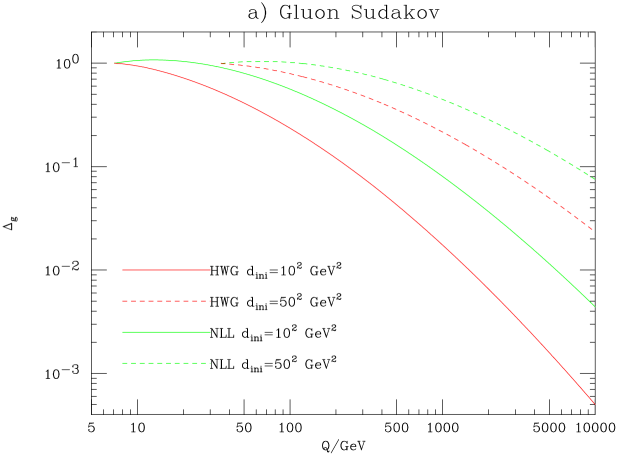
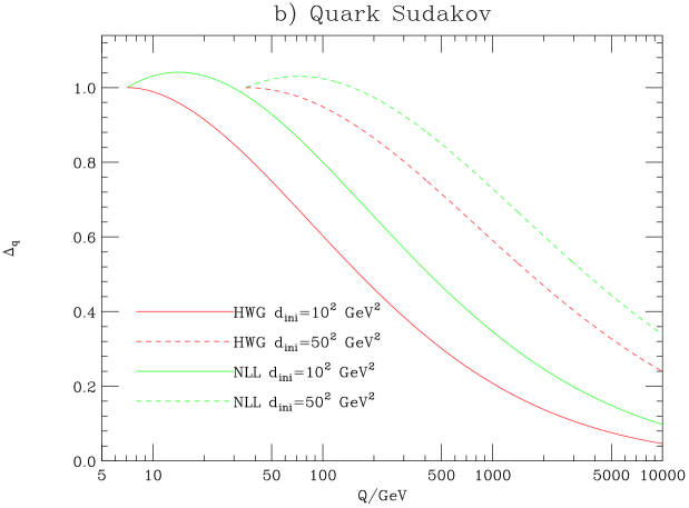
These differences both cause the HERWIG and PYTHIA Sudakov form factors to be smaller than the NLL ones. This is demonstrated in Fig. 3, which shows a comparison of the gluon and light quark Sudakov form factors from HERWIG and a NLL for different cut-off scales. The overall effect is a larger suppression of the higher multiplicity matrix elements for the HERWIG Sudakov form factor than the NLL one.
3.3 Choice of Scales
The CKKW algorithm specifies certain scales for the Sudakov form factor and . However, in principal, the functional form of the scale and the prefactor are not unique, and we have investigated a number of choices. One scale choice is the nodal values of (or equivalently the values of from the clustering), which should work well when an angular variable is used for the parton-shower evolution, as in HERWIG. However, we are not limited to this particular variable. The construction of a parton-shower history using the -algorithm and a particular recombination scheme provides a series of particles and pseudoparticles. Kinematic quantities can be constructed from the particle momenta. Thus, a second possible choice is the dot product of the four-momenta of the particles clustered, which is the same as the virtuality for massless particles and is the choice of initial conditions for the shower normally used in HERWIG. A third choice is the virtuality of the clustered pairs, which is the starting point for parton showers in PYTHIA.
The chosen scale is to be used as the starting point for the vetoed shower in the event generator. When reweighting by the Sudakov form factors, however, we allow for the possibility of a prefactor to the scale, which does not affect logarithmic behavior, but may have a quantitative impact nonetheless. If we consider, for example, then the choice of the starting scale for the HERWIG shower is which corresponds to a scale of in terms of the -measure. The same applies for the initial-state shower in Drell-Yan production at hadron colliders. However, the phase space of the HERWIG shower is such that no emission can occur with above , where is the scale variable in the parton shower. Therefore, in order to produce an emission up to the scale , the shower scale should be at least . We therefore leave the prefactor of the scale in the Sudakov form factors as a free parameter. Furthermore, we also allow for a minimum value of this parameter in terms of the cut-off used in the shower SCLCUT, where SCLCUT is the value of the matching scale . The choices are summarized below:
| (19d) | |||||
| (19e) | |||||
where is the -measure for the merging, and are the particles which are merged and is the virtuality of the pseudoparticle produced in the merging. We also allow for a minimum starting scale for the final-state parton shower, and a minimum starting scale of the initial-state parton shower
| (20a) | |||||
| (20b) | |||||
Finally, we need to specify the scale to be used in . The obvious choice is to use the same scale as in the form factors. However in HERWIG this is not done and the scale in is always lower than that in the shower. Therefore we have left the scale for as an additional free parameter and allow for a minimum value, such that
| (21d) | |||||
| (21e) | |||||
The various choices of ISCALE, QFACT(1-4) and AFACT(1-2) allow for flexibility in matching HERWIG or PYTHIA to a -ordered shower. It should be noted, however, that product of Sudakov form factors and factors of can significantly change the normalization of the final event sample. In practice, all of the distributions shown in later sections are renormalized for comparison with the standard event generators. The variation of scales and prefactors may also affect the truncation of the matrix element calculation, so that uncalculated contributions are relatively more important.
3.4 Treatment of the Highest Multiplicity Matrix Element
The CKKW algorithm applies the same procedure to all the matrix elements. However, in the numerical results presented by CKKW there is some additional ad hoc reweighting applied to increase the contributions from higher multiplicities. The necessity for this arises because of the practical limitation of calculating a matrix element of arbitrary multiplicity. The Sudakov reweighting of the matrix element and the vetoed parton showers are performed so as not to double-count contributions from higher multiplicities. However for the highest multiplicity matrix element, this is not the case. We consider three options, denoted by IFINAL. For IFINAL=1, we apply the reweighting but not the Sudakov reweighting and allow the parton shower to radiate freely from the scale at which the partons are produced. However, this allows the parton shower to produce higher -emissions than the matrix element. A better choice (IFINAL=3) is to apply the Sudakov weights for only the internal lines, start the parton shower at the scale at which the particle was produced and – instead of vetoing emission above the matching scale – veto emission above the scale of the particle’s last branching in the matrix element. Another choice (IFINAL=2), which is slightly easier to implement, is to only apply the Sudakov weight for the internal lines but start the shower at the normal scale for the parton shower and apply no veto at all.
4 Pseudo–Shower Procedure
The CKKW matching algorithm envisions a vetoed parton shower using a -ordered parton-shower generator. Both HERWIG and PYTHIA are not of this type. However, both of these generators have well–tested models of hadronization that are intimately connected to the parton shower, and we do not wish to discard them out of hand. For this reason, some aspects of the CKKW algorithm may not be suitable to a practical application of parton shower–matrix element matching.
4.1 Clustering
The naive approach to achieving a -veto in the HERWIG or PYTHIA shower would be to apply an internal veto on this quantity within the parton shower itself. To understand how this would work in practice, we will first review the kinematics of the PYTHIA shower for final-state radiation. A given branching is specified by the virtuality of the mother (selected probabilistically from the Sudakov form factor) and the energy fraction carried away by a daughter . In terms of these quantities, the combination represents the of the daughter parton to the mother in the small-angle approximation. A cut-off is determined by the minimal allowed invariant mass 1 GeV. Using Eqn. (15), the requirement of decreasing angle in the branching sequence can be reduced to
| (22) |
On the other hand, the -cluster variable expressed in the shower variables is:
| (23a) | |||||
| (23b) | |||||
The quantity Eq. (23b) would seem to be the natural variable to use for the veto within the shower. However, this is not as straightforward as it may seem. While the showering probability is determined assuming massless daughters, the final products conserve energy and momentum. In the soft-collinear limit, the minimum “” values will equal those obtained from -clustering of the final-state partons, but, in general, this will not be true. Since we are correcting the matrix element predictions to the soft-collinear regime of the parton shower, this approximation is valid. On the other hand, the restrictions from angular ordering via Eq. (22) favor whereas large values are more likely to be vetoed. After including the fact the invariant masses are decreasing, one can show that the first kinematically allowed branching has and , where is the minimum allowed value. The result is a suppression in the radiation in -cluster distributions in the vicinity of . Therefore, -clustering may be not be the preferred clustering algorithm, and other clustering schemes could be employed (see Ref.[38] for an extensive review of clustering schemes and their applicability) that is better suited to a particular event generator. In fact, both programs uses relative as a variable in . An alternative kinematic variable closely related to the relative is the LUCLUS measure [39]. According to the LUCLUS algorithm, clustering between two partons and is given by
| (24) |
instead of the relation of Eqn. 3. Expressed in terms of the parton-shower variables, where is the energy fraction carried by the daughter, and is the squared invariant mass of the mother, takes the form for final-state showers and for initial-state showers. In the pseudo-shower method, partons are clustered using the LUCLUS measure, and the internal veto of the parton shower is performed on the parton-shower approximation to .
4.2 Sudakov Form Factors
The original CKKW procedure uses the analytic form of the NLL Sudakov form factor. This is problematic for several reasons. First, as mentioned before, the PYTHIA shower is LL, which is related to the used in reweighting. Second, the “exact” NLL analytic expression is derived ignoring terms of order . In particular, energy and momentum are not conserved. This explains how the analytic Sudakov can have a value larger than 1 – without phase space restrictions, the subleading logarithms will become larger than the leading logarithms. It would be more consistent to require that the subleading terms are less than or equal to the leading one, but this will affect only rather large steps in virtuality.
In applying the CKKW algorithm to HERWIG, some ad hoc tuning of scale variables and prefactors is necessary to improve the matching. This is true also for an implementation using PYTHIA. In fact, the situation is further complicated by the dual requirements of decreasing mass and angle in PYTHIA, which is not commensurate with the analytical Sudakov form factor. An alternative approach is to use the parton shower of the generator itself to calculate the effect of the Sudakov form factors used to reweight the matrix element prediction. A method similar to the one described below was used in [32], but it is generalized here. It amounts to performing a parton shower on a given set of partons, clustering the partons at the end of the shower, and weighting the event by 0 or 1 depending on whether a given emission is above or below a given cut-off. When many partons are present at the matrix element level, several showers may be needed to calculate the full Sudakov reweighting. The algorithm for constructing the Sudakov reweighting is as follows (using partons as an example):
-
1.
Cluster the partons using some scheme. This generates a series of clustering values () as well as a complete history of the shower. Set , and .
-
2.
Apply a parton shower to the set of partons, vetoing any emissions with . Cluster the final-state partons, and reweight the event by 0 if , otherwise continue. If the weight is 0 at any time, then stop the algorithm and proceed to the next event.
-
3.
Use the parton-shower history to replace the two partons resolved at the scale with their mother. Rescale the event to conserve energy-momentum. This leaves a parton event. Set . If , go to step 2.
Equivalently, one could perform this procedure many times for each event and reweight by a factor equal to the number of events that complete the algorithm divided by the number of tries.
To see how the algorithm works in practice, consider a 3 parton event(). Application of the clustering algorithm will associate with or at the scale . For concreteness, assume the ()-combination has the smallest cluster value. A parton shower is applied to the partons starting at the scale where each parton is created (the scale for the and , and a lower scale for ), vetoing internally any emission with a cluster value . The final-state partons are then clustered, and the event is retained only if . If the event passes this test, the set of final-state partons is saved, and the () pair is replaced by the mother , leaving a event. A parton shower is applied to these partons vetoing internally any emission with a cluster value (i.e., no veto). The final-state partons are clustered, and the event is retained only if . If the event also passes this test, then the original set of showered partons have been suitably reweighted. The series of parton showers accounts for the Sudakov form factors on all of the parton lines between the scales and , eventually forming the full Sudakov reweighting.
4.3 Choice of Scales
The starting scales for showering the individual partons should match those scales used in the parton-shower generator. For PYTHIA, this choice is the invariant mass of the parton pair . For HERWIG, it is . Similarly, the scale and order for reweighting in should match the generators. PYTHIA uses the relative of the branching as the argument, whereas HERWIG uses the argument . Clustering in the variable is convenient, because then the nodal values from the clustering algorithm can be used directly.
4.4 Treatment of Highest Multiplicity Matrix Element
To treat the showering of the partons associated with the highest multiplicity at the matrix element level, we modify one of the steps in applying the Sudakov form factors numerically. Namely, in the first test for Sudakov suppression, we do not require . We loosen our requirement to be that , so that any additional radiation can be as hard as a radiation in the “hard” matrix-element calculation, but not harder. Furthermore, we veto emissions with , instead of . All other steps in the algorithm are unchanged.
5 Matching Results
In this section, we present matching results using matrix element calculations from MADGRAPH and parton showers from PYTHIA and HERWIG. Here, we will limit ourselves to presenting some simple distributions to demonstrate that the results are sensible and justify our recommended values of certain parameters and options.
The first subsection is devoted to collisions, where there is no complication from initial-state radiation of QCD partons. Also, there is a fixed center-of-mass energy, which allows a clear illustration of the matching. The second subsection is devoted to the hadronic production of weak gauge bosons, with all the ensuing complications.
5.1 Collisions
We will first present results for collisions at . This enables us to study the effects of various parameters and choices while only having final-state radiation. In particular it enables to see which are the best choices for a number of parameters related to the scales in the Sudakov form factors and .
The matrix element events were generated using MADGRAPH [33] and KTCLUS to implement the -algorithm with the definition given in Eqn. 3 for the -measure and the E-scheme. Matrix element calculations of up to 6 partons are employed, restricted to only QCD branchings (save for the primary one) and only containing light flavors of quarks and gluons.
Our results are cast in the form of differential distributions with respect to where and is the value of the -measure where the event changes from being an to an jet event. Since HERWIG and PYTHIA with matrix element corrections give good agreement with the LEP data for these observables, we compare the results of the different matching prescriptions to output of these programs.
For clarity, we recall the meaning of jet clustering and jet resolution. Experimentally, jet clustering is used to relate the high multiplicity of particles observed in collisions to the theoretical objects that can be treated in perturbation theory. Namely, the hadrons are related to the partons that fragment into them. Theoretically, we can apply clustering also to the partons with low virtuality to relate them to a higher energy scale and to higher virtuality partons. In the parton-shower picture, the daughters are related to mothers by the clustering.
Jet resolution is defined in terms of a resolution variable. It is sometimes more convenient to make the variable dimensionless, and this can be easily achieved in collisions by dividing the of a particular clustering by the center-of-mass energy of the collisions. The resolution variable sets a degree of fuzziness – structure below that energy scale is not to be discerned. In partons, the choice of corresponds to only one cluster (the itself), which is trivial and is ignored. The first interesting result occurs when there are three or more partons present, in which case there is a which separates a 2-cluster designation from a 3-cluster designation. This is the largest value of than can be constructed by clustering all of the partons. This particular value of would be denoted by the variable . If there are only 3 partons present, there is no choice of that can yield a 4-cluster designation. However, if 4 or more partons are present, then there is a choice of that is the boundary between a 3-cluster and a 4-cluster designation. This is the second largest that is constructed in clustering, and it would be denoted by a non-vanishing value of . Similarly, if 5 or more partons are present, a value of can be constructed, so on and so forth.
5.1.1 HERWIG-CKKW Results
Here, we show results based on applying -clustering, using the NLL Sudakov for reweighting, and HERWIG for performing the vetoed parton shower. We will demonstrate the dependence of our results on the choices of scale variables and prefactors before settling on an optimized choice.
The factors QFACT(1) and AFACT(1) modify the scale used in the Sudakov form factor and argument of respectively. QFACT(2) sets the minimal scale in the Sudakov. For simplicity, we set QFACT(1)=QFACT(2) and AFACT(1)=AFACT(2). We also set ISCALE=1, so that is the evolution variable. The effect of varying QFACT(1) and AFACT(1) on the parton-level differential distribution with NLL Sudakov form factors is shown in Fig. 4. The standard HERWIG prediction with the built-in matrix element correction is shown in magenta. In fact, the distribution is not very sensitive to the choices of parameters considered, particularly for smaller values of AFACT(1), except near the matching point of . Nonetheless, the choice of as the evolution variable and as the argument of yields the best agreement of the choices shown. The agreement with HERWIG for the differential distribution at parton level, Fig. 5, depends much more on the choice of scales, with QFACT(1)=1/2 and AFACT(1)=1/8 giving the best results. These particular results are for a matching scale of which corresponds to a value of . This is a very low value for the matching scale and therefore the difference between the different choices is enhanced. For either higher matching scales or centre-of-mass energies the differences are smaller. Using the HERWIG form factors (not shown here) gives worse agreement for these distributions.
The previous plots used the scale choice ISCALE=1. The dependence on the specific choice is demonstrated in Fig. 6 for the differential cross-section with respect to . The definition in terms of the -measure gives the best results, as we expected for the HERWIG (angular–ordered) algorithm. All the remaining results use this choice.
The effect of varying the minimum starting scale of the HERWIG parton shower, QFACT(3), together with the variation of the scale of , on the parton-level differential cross-section with respect to is shown in Fig. 7. In collisions the main effect of this parameter is to allow partons from the matrix element to produce more radiation, particularly those which are close to the cut-off in the matrix element. This tends to increase the smearing of the Durham jet measure for these partons causing more events from the matrix element to migrate below the matching scale after the parton shower. Despite the cut-off on emission above the matching scale in the parton shower, some emissions occur above the matching scale in the parton shower, and this can help to ensure a smooth matching. The choice of QFACT(3)=4.0 gives the best results.
So far, we have considered the and distributions, which depend on the properties of the hardest one or two additional jets generated by either the matrix element or parton shower, and thus are not very dependent on the treatment of the highest multiplicity matrix element – four additional jets in our numerical work. Rather than study a higher order distribution, we focus still on the distribution but vary the matrix element multiplicity. The rows of Fig. 8 show the results of truncating the matrix element results for different , while the columns show the dependence on the prefactor of the the scale in the argument for . In general the option IFINAL=3 gives the best results when only low multiplicity matrix elements are used. This corresponds to removing the Sudakov reweighting of the external partons (between a cluster scale and ) and performing the shower with a veto above the scale of the last emission in the matrix element. Also, both of the new prescriptions (IFINAL=2,3) perform better than the original CKKW prescription if only low jet multiplicity matrix elements are used. As the number of jets in the highest multiplicity matrix element increases the differences between the prescriptions decreases, because the relative importance of this contribution is decreased.
Up to this point, we have discussed all the parameters relevant for the simulation of in the HERWIG-CKKW procedure apart from the matching scale, . In principle the results should be relatively insensitive to the choice of this scale. In practice, there is a dependence, because (1) we must truncate the matrix element calculation at some order, and (2) the parton shower may or may not give an adequate description of physics below the cut-off. The effect of varying the matching scale on the differential cross-section with respect to is shown in Fig. 9 for and in Fig. 10 for GeV at parton level. In general the agreement between HERWIG and the results of the CKKW algorithm is good, and improves as the matching scale is increased. Similarly the agreement is better at GeV than .
Normally we would hope than the remaining differences at the matching scale would be smoothed out by the hadronization model. However as can be seen in Fig. 11 the HERWIG hadronization model distorts the parton-level results and produces a double peaked structure for the differential cross section with respect to at hadron level. This problem is due to the treatment of events where there is no radiation in the parton shower. In these events the HERWIG hadronization model produces large mass clusters and their treatment is sensitive to the parameters of the hadronization model which control the splitting of these clusters. Hopefully retuning these parameters would improve the agreement for this distribution. The results at GeV, shown in Fig.12, where the fraction of events with these massive clusters is smaller, are much closer to the original HERWIG result.
To summarize, the best results for the HERWIG-CKKW matching in collisions are obtained using NLL Sudakov form factors with a next-to-leading order .555We have not discussed the choice of the order of but NLO is required as this is always used in HERWIG. The best definition of the scale parameter is ISCALE=1, corresponding to as the evolution variable. The effect of varying the prefactors of the scales is less dramatic and while QFACT(1,2,3)=1/2 and AFACT(1,2)=1/4 are the best values these parameters can still varied in order to assess the effect of this variation on the results. The best choice for the treatment of the highest multiplicity matrix element is IFINAL=3 although provided sufficiently high multiplicity matrix elements are included the effect of this choice is small. Unfortunately, the hadron-level results are not as well-behaved as the parton-level ones, but this may be resolved by retuning the hadronization model. Though it has not been thoroughly investigated, this problem may be ameliorated when using PYTHIA with this prescription.
5.1.2 Pseudo-Shower Results
In this section, we show the results from the alternative scheme outlined in Sec. 4 based on using the Sudakov form factors and scale choices of the generators themselves. We show results in particular for the PYTHIA event generator, using the LUCLUS measure for clustering the partons to construct a parton-shower history. Clustering and matching is done on the LUCLUS variable. However, once a correction procedure has been applied, the results can be used for any collider predictions – one is not limited to studying LUCLUS-type variables for example. To facilitate comparison, we show final-state results based on the -clustering measure as in the previous discussion. The matrix element predictions are the same as those in the previous analysis (which more strictly adheres to the CKKW methodology), but have been clustered using the LUCLUS measure, so that they constitute a subset of those events.
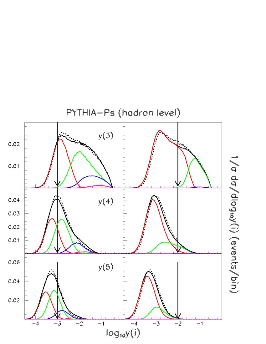
In the pseudo-shower approach, there are less free choices, so we will limit ourselves to the final results. Figure 13 shows the differential distributions for cut-offs of and , respectively, at the hadron level for and . Similar results (not shown) hold for . The cut-off used for generating the matrix element sample is shown as a vertical line in each of the distributions; however, an additional offset was added to each cut-off to account for any remaining mismatch between the parton-shower kinematics and the final-state parton/hadron kinematics. Removing this offset induces a radiation dip at the cut-off scale. A fixed value of GeV was used for this study. The default PYTHIA prediction including the matrix element correction is shown as the dashed-line. The corrected distribution is the solid line, and is a sum of matrix element predictions for 2 partons (red), 3 partons (green), 4 partons (blue), 5 partons (yellow) and 6 partons (magenta). It is interesting to compare the relative contributions of a given matrix element multiplicity for the different cut-offs. Note that, unlike in the CKKW-HERWIG procedure, there is a significant overlap of the different contributions. This is because the different matrix element samples are clustered in a different variable (the LUCLUS measure) and then projected into the -measure. The results generally agree with PYTHIA where they should, and constitute a more reliable prediction for the high- end of the distributions. For the lower cut-off, , the results are more sensitive to the treatment of the highest multiplicity matrix element, as indicated by the right tail of the matching predictions on the and distributions. For the higher cut-off, , the actual contribution of the 6 parton-matrix element is numerically insignificant, and there is little improvement over the PYTHIA result. Results at the parton level (not shown) are similar. Applying the same procedure to HERWIG (with the HERWIG choice of starting scales and argument for ) yields similar results.
5.2 Hadron-Hadron Collisions
Up to this point, we have benchmarked two procedures for matching matrix element calculations with parton showers – the HERWIG-CKKW procedure and the pseudo-shower procedure using HERWIG and PYTHIA. In this section, we apply these methods to particle production at hadron colliders. For the HERWIG-CKKW procedure, many of the choices of parameters and options were explored in the previous section. Here we focus on the additional parameters which are relevant to hadron collisions, although the effects of some of the parameters are different. In particular we have to make a choice of which variant of the -algorithm to use. For the pseudo-shower procedure, we apply the same method as for in a straight-forward fashion.
In hadron collisions, since the center-of-mass energy of the hard collision is not transparent to an observer, we study the differential distributions with respect to the square root of the -measure defined in Eqn. 4, as this is related to the differential cross section with respect to the of the jet.
5.2.1 HERWIG-CKKW Results
In order to assess the effects of the varying of the scales for and the minimum starting scale for the shower in hadron-hadron collisions we started by studying electroweak gauge boson production using the monotonic -scheme and a matching scale at the Tevatron for a centre-of-mass energy of TeV. The events we are considering were generated including the leptonic decay of the W with no cuts on the decay leptons. The events were also generated including the leptonic decay of the gauge boson and included the contribution of the photon exchange diagrams. To control the rise in the cross section at small invariant masses of the lepton pair, , a cut was imposed requiring GeV.
The differential cross section with respect to is shown in Fig. 14 for W production and for Z production in Fig. 15. The differential cross section with respect to for W production is shown in Fig. 16. The results for for W production show good agreement between HERWIG and the CKKW result for all the parameters, however the mismatch at the matching scale increases as QFACT(3,4) increases. The is due to the same effect we observed in collision, i.e. more smearing of the one jet matrix element result causing more of these events to migrate below the matching scale. However the results for both Z production and in W production show a much larger discrepancy at the matching scale. In both cases there is a depletion of radiation below the matching scale with respect to the original HERWIG result. This is not seen in the distribution for W production as here the initial-state parton shower always starts at the W mass.666In practice this is smeared with the Breit-Wigner distribution due to the width of the W. However the parton shower for Z production often starts at the cut-off on the lepton pair mass and the parton shower of the matrix element often starts at a much lower scale. One possible solution to this problem, at least for W production, is to always start the initial-state parton shower at the highest scale in the process. In Z production however this cannot solve the problem of lack of radiation from events which have a low mass lepton pair.
The best solution to this problem is to decouple the minimum starting scale for the initial- and final-state parton showers. In practice we want to use a low value for the final-state shower in order to reduce the smearing of the higher multiplicity matrix elements and a high value for the initial-state shower to avoid the problem of the radiation dip below the matching scale.
5.2.2 Pseudo-Shower Results
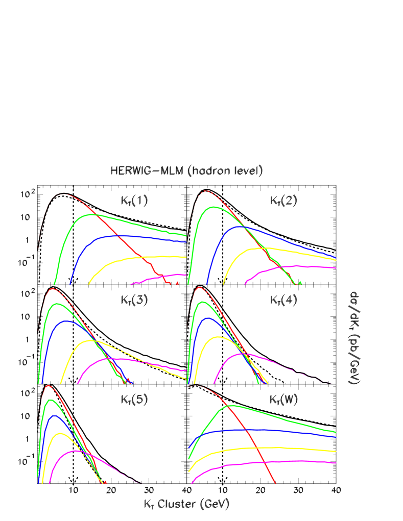
In this section, we show the results of using the alternative scheme outlined in Sec. 4. We show results for the PYTHIA and HERWIG event generators applied to production at the Tevatron, using the LUCLUS measure for clustering the partons to construct a parton-shower history. Again, since final results should not depend on the correction methodology, we show results based on the -clustering measure as in the previous discussion. In all cases, we use a factorization scale (which sets the upper scale for parton showers) equal to the transverse mass of the boson: .
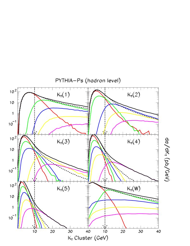
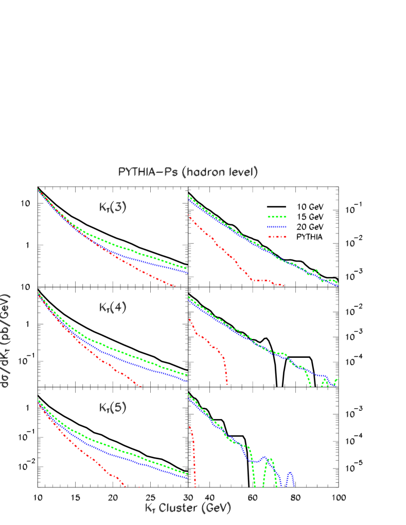
Figure 17 shows the differential -distributions for a cut-off of GeV, using the pseudo-shower procedure with PYTHIA to generate the parton shower. Similar results hold for cut-offs of 15 and 20 GeV used in this study. As for the case, these distributions are constructed from fully hadronized events. For the case of hadronic collisions, this requires that partons from the underlying event and the hadronic remnants of the beam particles are not included in the correction. In PYTHIA and HERWIG, such partons can be identified in a straight-forward manner. The default PYTHIA prediction including the matrix element correction is shown as the dashed line. The corrected distribution is in black, and is a sum of matrix element predictions for 0 partons (red), 1 parton (green), 2 partons (blue), 3 partons (yellow) and 4 partons (magenta). The largest -cluster value, which roughly corresponds to the highest jet, agrees with the PYTHIA result, but is about higher by GeV. Such an increase is reasonable, since matrix element corrections from two or more hard partons is not included in PYTHIA. The deviations from default PYTHIA become greater when considering higher -cluster values: is roughly an order of magnitude larger in the pseudo-shower method at GeV. The transverse momentum of the boson, however, is not significantly altered from the PYTHIA result, increasing by about at GeV. Of course, larger deviations will be apparent at higher values of transverse momentum.
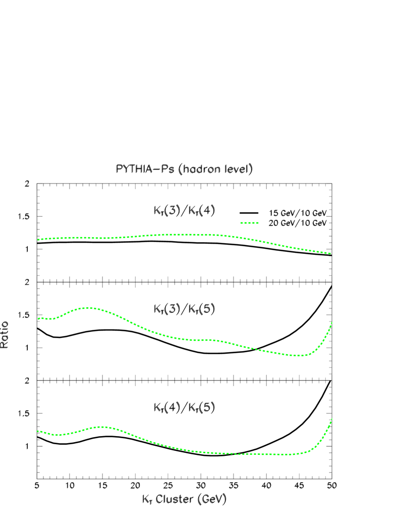
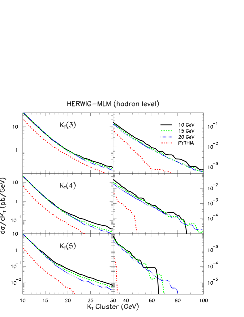
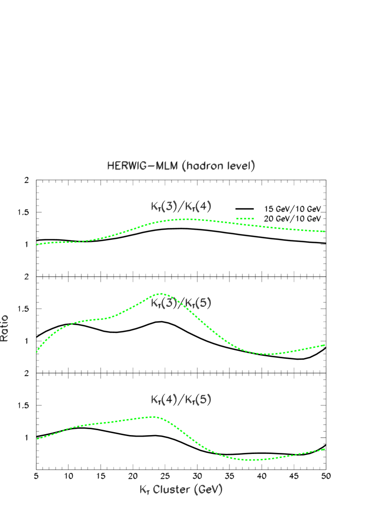
The dependence on the cut-off is illustrated in Figure 18, which shows the distributions for the 3rd, 4th, and 5th largest value of -cluster for the different choices of matching scale: 10 GeV (solid), 15 GeV (dashes), and 20 GeV (dots). The default PYTHIA prediction with the matrix element correction (dot-dash) is shown for comparison. For GeV, the predictions are robust, though there is a noticeable dependence with the matching scale for GeV. The distribution is generated purely from parton showering of the other parton configurations. The largest variation among the predictions occurs around GeV, corresponding to the largest cut-off, where the differential cross section ranges over a factor of 3. Thus, for absolute predictions, the choice of matching scale introduces a significant systematic bias. On the other hand, most likely the data will be used to normalize distributions with relatively loose cuts. Figure 19 shows the ratio of the distributions shown in Fig. 18 with respect to the distribution with a cut-off of 10 GeV, which exhibits far less variation with the choice of matching scale. The ratio of the distribution for a cut-off of 15 GeV to 10 GeV is shown (solid) and for 20 GeV to 10 GeV (dashed). The most significant variation, about 60% for GeV, occurs in the ratio , which is sensitive to the treatment of the highest multiplicity matrix element ( partons here), and would be expected to show the greatest variation. The variation is smaller for above the largest matching scale (20 GeV).
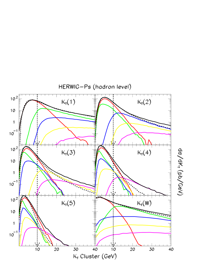
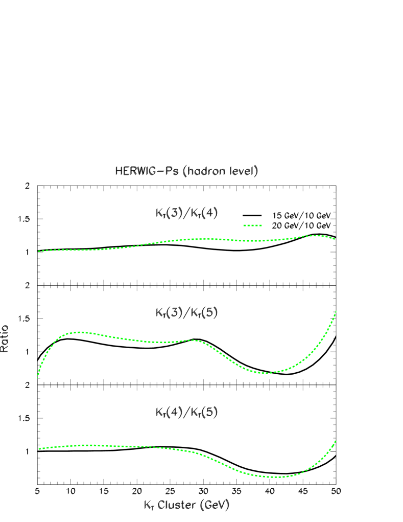
To test the whole pseudo-shower methodology, we now show results based on applying the same algorithm with the HERWIG event generator. A different starting scale and argument for is used, as noted previously. The comparative -distributions are shown in Figure 20. Similar results hold for the cut-off values of 15 and 20 GeV used in this study, and are not shown here for brevity. The results are similar in nature to those from PYTHIA, though the spectra are are typically softer at the tail of the distributions. Note that the pseudo-shower HERWIG results are compared to PYTHIA (not HERWIG) with the tuned underlying event model. Focusing attention on Figs. 21 and 22, which show the distributions and and their ratios, we observe a smaller variation than for the PYTHIA case. The variation for in the range of 10 GeV is approximately 30%. In general, the dependence on matching scale is smaller than for the PYTHIA results, both for the absolute shapes and ratios.
6 Comparison to the MLM Approach
Recently, a less complicated method was suggested for adding parton showers to parton matrix element calculations [40]. We denote this as the MLM method. The resulting events samples were meant for more limited applications, but it is worth commenting on the overlap between the approaches.
The MLM method consists of several steps:
-
1.
Generate events of uniform weight for partons at the tree level with cuts on , , and , where and denote partons. The PDF’s and are evaluated at the factorization scale or . The uniform weight of the events is the given by the total cross section divided by the number of events: .
-
2.
Apply a parton shower using HERWIG with a veto on , where is the HERWIG approximation to the relative as described earlier. By default, the starting scale for all parton showers is given by , where and are color–connected partons.
-
3.
The showered partons are clustered into jets using a cone algorithm with parameters and . If , the event is reweighted by 0. If (this is the inclusive approach), the event is reweighted by 1 if each of the original partons is uniquely contained within a reconstructed jet. Otherwise, the event is reweighted by 0.
-
4.
At the end of the procedure, one is left with a sub-sample of the original events with total cross section , where are the number of events accepted (reweighted by 1).
The method is well motivated. It aims to prevent the parton shower from generating a gluon emission that is harder than any emission already contained in the “hard” matrix-element calculation. The cuts on and play the role of the clustering cuts on or (see Eq. (4)). Clearly, the same cuts applied to the matrix element calculation are used to control the amount of radiation from the parton shower. However, a full clustering of the event is not necessary, since no Sudakov form factors are applied on internal lines, and HERWIG already has a default choice of starting scales. Based on the understanding of the numerical method for applying the Sudakov reweighting, it is clear that the final step of rejecting emissions that are too hard with respect to the matrix element calculation is the same as applying a Sudakov form factor to the external lines only. With respect to the internal lines, the reweighting coming from an internal line in the parton-shower approach, given by the product of the Sudakov form factor and the branching factor , is to be compared to the weight in the MLM approach. The size of any numerical difference between these factors is not obvious.
To facilitate a direct comparison between the methods, we substitute the cuts on and with a cut on the minimum -cluster value as in the original CKKW proposal. The jet-parton matching (step 3) is further replaced by the requirement that the st value of after clustering the showered partons is less than the th value of from clustering the original partons, i.e . We will experiment with the choice of a veto on the parton shower, using either or for the internal HERWIG veto.
The resulting -distributions are shown in Figure 23. Similar results hold for the cut-off values of 15 and 20 GeV also used in this study, but not shown here. A comparison of the -distributions for different choices of matching scales is shown in Fig. 24. While there are notable differences with the previous approaches, the matching is nonetheless robust. The distribution indicates some enhancement-depletion of radiation above-below the matching scale, becoming more noticeable as the matching scale is increased. However, the distribution does not suffer from this effect. The variation with the matching scale is smaller than in the previous approaches, and is most noticeable for GeV.
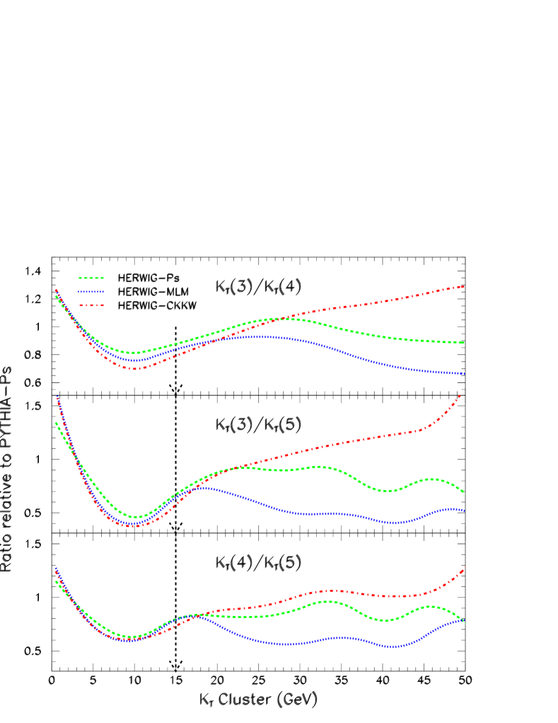
Finally, Fig. 26 shows a comparison of the ratios using the pseudo-shower method with HERWIG the MLM method with HERWIG, and the HERWIG-CKKW method, all relative to the PYTHIA pseudo-shower result. The cut-off used for this comparison is 15 GeV. Below this scale, the two HERWIG distributions are almost identical, and there is a significant difference with PYTHIA for distributions involving – which is generated by the parton shower. Above the cut-off, the pseudo-shower procedure and the MLM procedure are in close agreement, and are on the order of 20% higher than the HERWIG pseudo-shower results. This, then, is a good estimate in the range of uncertainty in these predictions.
7 Discussion and Conclusions
In this work, we report on our exploration of matching matrix element predictions with parton showers using a methodology close to the CKKW algorithm suggested in [29, 30]. In sum, we have compared three different procedures: (1) a slightly expanded version of the CKKW procedure using HERWIG as the parton-shower generator (but not limited in principal to HERWIG) and exploiting the freedom to choose scales and cut-offs; (2) a version of the CKKW procedure relying on pseudo-showers and matched closely to the scales and cut-offs of PYTHIA and HERWIG; and (3) a much simpler procedure based on the approach of M. Mangano. All three of the procedures yield reasonable results.
The HERWIG-CKKW procedure uses all of the elements of the original CKKW procedure, but expands upon them. Several choices of scale were investigated as starting points for the vetoed parton shower, and a wide range of prefactors were explored as arguments to the analytic NLL Sudakov form factor and . The variation of the results with these choices is shown in the figures. Optimized choices were settled upon based on the smoothness of distributions, the agreement with HERWIG where expected, and the apparent improvement over the default HERWIG predictions. While this appears to be a tuning, the final choices are easily justifiable. Since HERWIG is an angular-ordered shower, a variable such as -cluster values is well suited as a starting point for the HERWIG shower. Because of the details of the HERWIG shower, a prefactor of for the scale used in the Sudakov form factor is understandable, as well as a prefactor of for the scale used in evaluating . The results presented are better at the parton level than at the hadron level, which may require some tuning of the HERWIG hadronization model. These effects become less important when considering scattering processes at higher energies or when the cut-offs are larger.
The pseudo-shower procedure uses the Sudakov form factors of HERWIG and PYTHIA to numerically calculate the Sudakov suppression. Since the Sudakov form factor is a probability distribution for no parton emissions, the suppression factor can be determined by starting showers from different stages of the parton-shower history and discarding those events with emissions above a given cut-off. Because of the nature of this approach, there is less tuning of parameters. To match the argument used in by default in HERWIG and PYTHIA, a different clustering scheme was used: clustering or LUCLUS-clustering. Final results at the hadron level are shown in the figures. In general, the hadron-level results are better than the parton-level ones. The use of LUCLUS over KTCLUS was driven by the kinematics of the PYTHIA shower. We have not checked whether KTCLUS works as well or better for the HERWIG results, and we leave this for future investigation. We should also investigate the advantages of using the exact clustering scheme of the individual generators: invariant mass and angular ordering for PYTHIA or just angular ordering for HERWIG. Also, since this work began, a new model of final-state showering was developed for PYTHIA which is exactly of the LUCLUS type. This should also be tested, and ideally the -ordered shower could be expanded to include initial-state radiation. This is beyond the stated aims of this work, which was to investigate the use of HERWIG and PYTHIA with minor modifications.
The MLM procedure is a logical extension of the procedure develop by M. Mangano for adding partons showers to +multijet events. It entails -clustering the parton-level events, adding a parton shower (with HERWIG in practice, but not limited to it), and rejecting those events where the parton shower generates a harder emission (in the -measure) than the original events. This approach yields a matching which is almost as good as the more complicated procedures based on the CKKW procedures explored in this work. The reason is not a pure numerical accident. The MLM procedure rejects events (equivalently, reweights them to zero weight) when the parton shower generates an emission harder than the lowest value of the given kinematic configuration. This is equivalent to the first step of the pseudo-shower procedure in the calculation of the Sudakov suppression when applied to the highest multiplicity matrix element. The remaining difference is in the treatment of the internal Sudakov form factors and the argument of . The agreement between the pseudo-shower and MLM procedures implies that the product of Sudakov form factors on internal lines with the factors of evaluated at the clustering scale is numerically equivalent to the product of factors evaluated at the hard scale. It is worth noting that, for the process at hand, , only two of the cluster values can be very close to the cut-off, and thus only two of the values can be very large. Also, at the matching scales considered in this study, GeV, with a factorization scale on the order of , , a fixed order expansion is of similar numerical reliability as the “all-orders” expansion of a resummation calculation. In fact, the resummation (parton shower) expansion is ideally suited for , whereas the fixed order expansion is best applied for . The matching scales used in this study straddle these extremes.
Based on the study of these three procedures, we can make several statements on the reliability of predicting the shapes and rates of multijet processes at collider energies.
-
1.
The three matching procedures studied here can be recommended. They are robust to variation of the cut-off scale.
-
2.
The relative distributions in , for example, are reliably predicted.
-
3.
The variation in the relative distributions from the three procedures depends on the variable. For variables within the range of the matrix elements calculated, the variation is 20%. For variables outside this range, which depend on the truncation of the matrix element calculation, the variation is larger 50%. Of course, it is important to study the experimental observables to correctly judge the senstivity to the cut-off and methodology of matching.
-
4.
More study is needed to determine the best method for treating the highest multiplicity matrix-element contributions.
-
5.
The subject of matching is far from exhausted. The procedures presented here yield an improvement over previous matching prescriptions. However, these methodologies are an interpolation procedure.
Acknowledgments
PR thanks S. Gieseke, F. Krauss, M. Mangano, M. Seymour, B. Webber and members of the Cambridge SUSY working group for many useful discussions about the CKKW algorithm. SM thanks T. Sjöstrand for similar discussions. PR and SM both thank J. Huston for discussion, encouragement and for asking the difficult questions. This work was started at the Durham Monte Carlo workshop and presented at the Durham ’Exotics at Hadron Colliders’, Fermilab Monte Carlo, Les Houches and CERN MC4LHC workshops. PR would like to thank the organisers of these workshops and the Fermilab theory and computing divisions for their hospitality during this work. SM thanks the Stephen Wolbers and the Fermilab Computing Division for access to the Fixed Target Computing Farms. PR gives similar thanks to the support term at the Rutherford lab CSF facility.
References
- [1] T. Sjostrand et. al., High-Energy-Physics Event Generation with PYTHIA 6.1, Comput. Phys. Commun. 135 (2001) 238–259, [http://arXiv.org/abs/hep-ph/0010017].
- [2] T. Sjostrand, L. Lonnblad, and S. Mrenna, PYTHIA 6.2: Physics and Manual, http://arXiv.org/abs/hep-ph/0108264.
- [3] T. Sjostrand, L. Lonnblad, S. Mrenna, and P. Skands, Pythia 6.3 physics and manual, hep-ph/0308153.
- [4] T. Sjostrand and M. Bengtsson, The Lund Monte Carlo for Jet Fragmentation and Physics: JETSET Version 6.3: An Update, Comput. Phys. Commun. 43 (1987) 367.
- [5] M. Bengtsson and T. Sjostrand, Parton showers in leptoproduction events, Z. Phys. C37 (1988) 465.
- [6] E. Norrbin and T. Sjostrand, Qcd radiation off heavy particles, Nucl. Phys. B603 (2001) 297–342, [hep-ph/0010012].
- [7] G. Miu and T. Sjostrand, W Production in an Improved Parton Shower Approach, Phys. Lett. B449 (1999) 313–320, [hep-ph/9812455].
- [8] G. Corcella et. al., HERWIG 6: An Event Generator for Hadron Emission Reactions with Interfering Gluons (including supersymmetric processes), JHEP 01 (2001) 010, [http://arXiv.org/abs/hep-ph/0011363].
- [9] G. Corcella et. al., HERWIG 6.5 Release Note, hep-ph/0210213.
- [10] M. H. Seymour, Photon Radiation in Final-State Parton Showering, Z. Phys. C56 (1992) 161–170.
- [11] M. H. Seymour, Matrix Element Corrections to Parton Shower Simulation of Deep Inelastic Scattering, . Contributed to 27th International Conference on High Energy Physics (ICHEP), Glasgow, Scotland, 20-27 Jul 1994.
- [12] G. Corcella and M. H. Seymour, Matrix Element Corrections to Parton Shower Simulations of Heavy Quark Decay, Phys. Lett. B442 (1998) 417–426, [hep-ph/9809451].
- [13] G. Corcella and M. H. Seymour, Initial-State Radiation in Simulations of Vector Boson Production at Hadron Colliders, Nucl. Phys. B565 (2000) 227–244, [hep-ph/9908388].
- [14] M. H. Seymour, Matrix Element Corrections to Parton Shower Algorithms, Comp. Phys. Commun. 90 (1995) 95–101, [hep-ph/9410414].
- [15] J. Andre and T. Sjostrand, A matching of matrix elements and parton showers, Phys. Rev. D57 (1998) 5767–5772, [hep-ph/9708390].
- [16] S. Mrenna, Higher Order Corrections to Parton Showering from Resummation Calculations, hep-ph/9902471.
- [17] C. Friberg and T. Sjostrand, Some Thoughts on how to Match Leading Log Parton Showers with NLO Matrix Elements, hep-ph/9906316.
- [18] J. C. Collins, Subtraction Method for NLO Corrections in Monte Carlo Event Generators for Leptoproduction, JHEP 05 (2000) 004, [hep-ph/0001040].
- [19] J. C. Collins and F. Hautmann, Soft Gluons and Gauge-Invariant Subtractions in NLO Parton- Shower Monte Carlo Event Generators, JHEP 03 (2001) 016, [hep-ph/0009286].
- [20] Y. Chen, J. C. Collins, and N. Tkachuk, Subtraction Method for NLO Corrections in Monte-Carlo Event Generators for Z Boson Production, JHEP 06 (2001) 015, [hep-ph/0105291].
- [21] B. Potter, Combining QCD Matrix Elements at Next-to-Leading Order with Parton Showers, Phys. Rev. D63 (2001) 114017, [hep-ph/0007172].
- [22] B. Potter and T. Schorner, Combining Parton Showers with Next-to-Leading Order QCD Matrix Elements in Deep-Inelastic e p Scattering, Phys. Lett. B517 (2001) 86–92, [hep-ph/0104261].
- [23] M. Dobbs and M. Lefebvre, Unweighted Event Generation in Hadronic W Z Production at Order , Phys. Rev. D63 (2001) 053011, [hep-ph/0011206].
- [24] M. Dobbs, Incorporating Next-to-Leading Order Matrix Elements for Hadronic Diboson Production in Showering Event Generators, Phys. Rev. D64 (2001) 034016, [hep-ph/0103174].
- [25] M. Dobbs, Phase Space Veto Method for Next-to-Leading Order Event Generators in Hadronic Collisions, Phys. Rev. D65 (2002) 094011, [hep-ph/0111234].
- [26] S. Frixione and B. R. Webber, Matching NLO QCD Computations and Parton Shower Simulations, JHEP 06 (2002) 029, [hep-ph/0204244].
- [27] S. Frixione and B. R. Webber, The MC@NLO event generator, hep-ph/0207182.
- [28] Y. Kurihara et. al., QCD Event Generators with Next-to-Leading Order Matrix- Elements and Parton Showers, hep-ph/0212216.
- [29] S. Catani, F. Krauss, R. Kuhn, and B. R. Webber, QCD Matrix Elements + Parton Showers, JHEP 11 (2001) 063, [hep-ph/0109231].
- [30] F. Krauss, Matrix Elements and Parton Showers in Hadronic Interactions, JHEP 08 (2002) 015, [hep-ph/0205283].
- [31] L. Lonnblad, Combining Matrix Elements and the Dipole Cascade Model, Acta Phys. Polon. B33 (2002) 3171–3176.
- [32] L. Lonnblad, Correcting the Colour-Dipole Cascade Model with Fixed Order Matrix Elements, JHEP 05 (2002) 046, [hep-ph/0112284].
- [33] F. Maltoni and T. Stelzer, MadEvent: Automatic event generation with MadGraph, hep-ph/0208156.
- [34] M. L. Mangano, M. Moretti, F. Piccinini, R. Pittau, and A. D. Polosa, ALPGEN, a Generator for Hard Multiparton Processes in Hadronic Collisions, hep-ph/0206293.
- [35] E. Boos et. al., Generic user process Interface for Event Generators, hep-ph/0109068.
- [36] T. Gleisberg et. al., Sherpa 1.alpha, a proof-of-concept version, hep-ph/0311263.
- [37] S. Catani, Y. L. Dokshitzer, M. H. Seymour, and B. R. Webber, Longitudinally Invariant -Clustering Algorithms for Hadron-Hadron collisions, Nucl. Phys. B406 (1993) 187–224.
- [38] S. Moretti, L. Lonnblad, and T. Sjostrand, New and Old Jet Clustering Algorithms for electron positron events, JHEP 08 (1998) 001, [hep-ph/9804296].
- [39] T. Sjostrand, The Lund Monte Carlo for jet physics, Comput. Phys. Commun. 28 (1983) 229.
- [40] M. Mangano, Exploring theoretical systematics in the ME-to-shower MC merging for multijet process, E-proceedings of Matrix Element/Monte Carlo Tuning Working Group, Fermilab, November 2002.