Methods for extracting Higgs boson signals at a 1 TeV center-of-mass energy $e^{+}e^{-}$ linear collider are described. In addition, estimates are given for the accuracy with which branching fractions can be measured for Higgs boson decays to $b\bar{b}$, $WW$, $gg$, and $\gamma\gamma$.

1 Introduction

The precision measurement of the Higgs boson couplings to fermions and gauge bosons is one of the most important goals of an $e^{+}e^{-}$ linear collider. These measurements will distinguish between different models of electroweak symmetry breaking, and can be used to extract parameters within a specific model, such as supersymmetry. Most linear collider Higgs studies have been made assuming a center-of-mass energy of 0.35 TeV, where the Higgsstrahlung cross-section is not too far from its peak value for Higgs boson masses less than 250 GeV . Higgs branching fraction measurements with errors of $2-10$% can be achieved at $\sqrt{s}=0.35$ TeV for many Higgs decay modes, and the total Higgs width can be measured with an accuracy of $5-13$% if the $\sqrt{s}=0.35$ TeV data is combined with $WW$ fusion production at $\sqrt{s}=0.50$ TeV[1]. These measurement errors are very good, but is it possible to do better?

In the CLIC study of physics at a 3 TeV $e^{+}e^{-}$ linear collider it was recognized that rare Higgs decay modes such as $h\rightarrow\mu^{+}\mu^{-}$ could be observed using Higgs bosons produced through $WW$ fusion[2, 3]. This is possible because the cross-section for Higgs production through $WW$ fusion rises with center-of-mass energy, while the design luminosity of a linear collider also rises with energy. One doesn’t have to wait for a center-of-mass energy of 3 TeV, however, to take advantage of this situation. Already at $\sqrt{s}=1$ TeV the cross-section for Higgs boson production through $WW$ fusion is two to four times larger than the Higgsstrahlung cross-section at $\sqrt{s}=0.35$ TeV, and the linear collider design luminosity is two times larger at $\sqrt{s}=1$ TeV than at $\sqrt{s}=0.35$ TeV[4]. Table 1 summarizes the Higgs event rates at $\sqrt{s}=0.35$ and 1 TeV for several Higgs boson masses.

Table 1: Number of inclusive Higgs events assuming an initial state electron polarization of -80% and integrated luminosities of 500 (1000) fb^-1 for $\sqrt{s}=350$ (1000) GeV. Effects from beamstrahlung and initial state radiation are included assuming the NLC machine design.

		Higgs Mass (GeV)
$\sqrt{s}$ (GeV)	$e^{+}_{\rm pol}$ (%)	120	140	160	200
350	0	110280	89150	69975	37385
350	+50	159115	128520	100800	53775
1000	0	386550	350690	317530	259190
1000	+50	569750	516830	467900	382070

In this report methods for extracting Higgs boson signals at a 1 TeV center-of-mass energy $e^{+}e^{-}$ linear collider are presented, along with estimates of the accuracy with which the Higgs boson cross-section times branching fractions, $\sigma\cdot B_{xx}$, can be measured. All results and figures at $\sqrt{s}=1$ TeV assume 1000 fb^-1 luminosity, -80% electron polarization, and +50% positron polarization.

2 Event Simulation

The Standard Model backgrounds from all 0,2,4,6-fermion processes and the top quark-dominated 8-fermion processes are generated at the parton level using the WHIZARD Monte Carlo[5]. In the case of processes such as $\mbox{$e^{+}e^{-}$}\rightarrow\mbox{$e^{+}e^{-}$}f\bar{f}$ the photon flux from real beamstrahlung photons is included along with the photon flux from Weiszäcker-Williams low-$q^{2}$ virtual photons. The production of the Higgs boson and its subsequent decay to $b\bar{b}$ and $\tau^{+}\tau^{-}$ is automatically included in WHIZARD in the generation of the 4-fermion processes $\mbox{$e^{+}e^{-}$}\rightarrow f\bar{f}b\bar{b}$ and $\mbox{$e^{+}e^{-}$}\rightarrow f\bar{f}\tau^{+}\tau^{-}$. For other Higgs decay modes the WHIZARD Monte Carlo is used to simulate $\mbox{$e^{+}e^{-}$}\rightarrow f\bar{f}h$ and the decay of the Higgs boson is then simulated using PYTHIA[6]. The PYTHIA program is also used for final state QED and QCD radiation and for hadronization. The CIRCE parameterization[7] of the NLC design[4] at $\sqrt{s}=1$ TeV is used to simulate the effects of beamstrahlung. For the detector Monte Carlo the SIMDET V4.0 simulation[8] of the TESLA detector[9] is utilized.

3 Measurement of $\bf\sigma\cdot B_{xx}$ at $\bf\sqrt{s}=1$ TeV

Results will be presented for the Higgs decay modes $h\rightarrow b\bar{b},\ WW,\ gg,\ \gamma\gamma$. The $h\rightarrow c\bar{c}$ decay is not studied since a detailed charm-tagging analysis is beyond the scope of this paper; however it might be interesting for charm-tagging experts to pursue this decay mode at $\sqrt{s}=1$ TeV. The $h\rightarrow\tau^{+}\tau^{-}$ decay is not considered since the neutrinos from the decays of the taus severely degrade the Higgs mass reconstruction.

Higgs events are preselected by requiring that there be no isolated electron or muon, and that the angle of the thrust axis $\theta_{\rm thrust}$, visible energy $E({\rm visible})$, and total visible transverse momentum $p_{T}({\rm visible})$ satisfy

$$|\cos{\theta_{\rm thrust}}|<0.95,\quad$$

$$100<E({\rm visible})<400\ {\rm GeV}, 20<p_{T}({\rm visible})<500{\rm GeV}.$$ (1)

Other event variables which will be used in the Higgs event selection include the total visible mass $M({\rm visible})$, the number of charged tracks $N({\rm chg})$, the number of large impact parameter charged tracks $N({\rm imp})$, and the number of jets $N({\rm jet})$ as determined by the PYCLUS algorithm of PYTHIA with parameters MSTU(46)=1 and PARU(44)=5.

3.1 $\bf h\rightarrow b\bar{b}$

Decays of Higgs bosons to $b$ quarks are selected by requiring:

$$6\leq N({\rm chg})\leq 19,\quad 7\leq N({\rm imp})\leq 19,$$

$$2\leq N({\rm jet})\leq 3,\quad M_{h}-10\ {\rm GeV}<M({\rm visible})<M_{h}+6\ {\rm GeV},$$ (2)

where $M_{h}$ is the Higgs boson mass measured at $\sqrt{s}=350$ GeV. Histograms of $M({\rm visible})$ are shown in Fig. 1 assuming Higgs boson masses of 120 and 200 GeV. Most of the non-Higgs SM background in the left-hand plot is due to $\mbox{$e^{+}e^{-}$}\rightarrow e\nu W,\ eeZ,\ \nu\nu Z$, while the non-Higgs background in the right-hand plot is mostly $\gamma\gamma\rightarrow WW$. The statistical accuracy for cross-section times branching ratio, $\sigma\cdot B_{bb}$, is shown in the first row of Table 2, along with results for $M_{h}=115,\ 140,\ {\rm and}\ 160$ GeV.

The Higgs background makes up 1.2% of the events in the left-hand plot that pass all cuts, and of these 70% are $c\bar{c}$, 20% are $gg$, 5% are $WW^{*}$, and 5% are $ZZ^{*}$. The Higgs background is small enough that Higgs branching fraction measurements from $\sqrt{s}=350$ GeV can be used to account for this background without introducing a significant systematic error. The non-Higgs background should be calculated with an accuracy of 1 to 2% to keep the non-Higgs background systematic error below the statistical error.

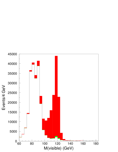
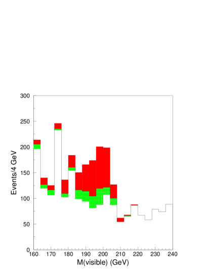
Figure 1: Histograms of $M({\rm visible})$ following $b\bar{b}$ selection cuts for background and signal assuming $M_{h}=120$ GeV (left) and $M_{h}=200$ GeV (right). The histograms contain non-Higgs SM background (white), $h\rightarrow b\bar{b}$ (red) and other Higgs decays (green).

3.2 $\bf h\rightarrow\gamma\gamma$

Decays of Higgs bosons to photon pairs are selected by requiring:

$$N({\rm chg})=0,\quad N({\rm imp})=0,$$

$$N({\rm jet})=2,\quad M_{h}-2\ {\rm GeV}<M({\rm visible})<M_{h}+1\ {\rm GeV}.$$ (3)

Histograms of $M({\rm visible})$ are shown in Fig. 2 assuming Higgs boson masses of 120 and 160 GeV. The SM background is almost entirely $\mbox{$e^{+}e^{-}$}\rightarrow\nu\nu\gamma\gamma$.

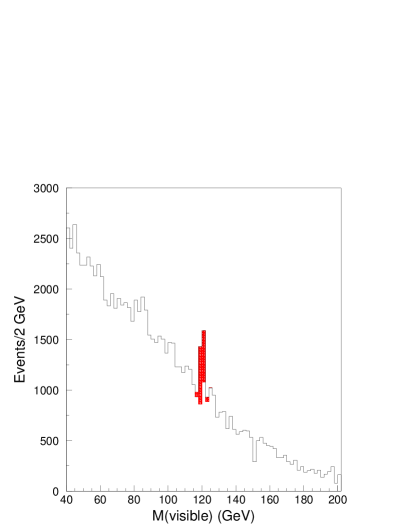
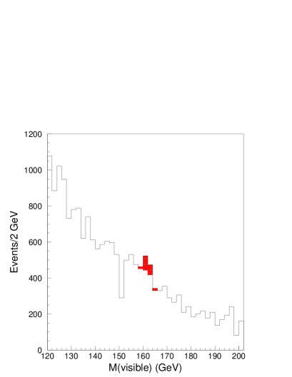
Figure 2: Histograms of $M({\rm visible})$ following $\gamma\gamma$ selection cuts for background and signal assuming $M_{h}=120$ GeV (left) and $M_{h}=160$ GeV (right). The histograms contain non-Higgs SM background (white) and $h\rightarrow\gamma\gamma$ (red).

3.3 $\bf h\rightarrow WW,\ \ gg$

Decays of Higgs bosons to $WW$ or $WW^{*}$ are selected by requiring:

$$16\leq N({\rm chg})\leq 44,\quad N({\rm imp})\leq 6,$$

$$4\leq N({\rm jet})\leq 5,\quad M_{h}-10\ {\rm GeV}<M({\rm visible})<M_{h}+6\ {\rm GeV}.$$ (4)

The histogram of $M({\rm visible})$ following the $WW$ cuts is shown in the left-hand side of Fig. 3 for a Higgs boson mass of 120 GeV. The non-Higgs SM background is mostly $\mbox{$e^{+}e^{-}$}\rightarrow e\nu W$. There is also a substantial Higgs boson background consisting of $h\rightarrow gg$ (63%), $h\rightarrow bb$ (14%), $h\rightarrow cc$ (12%) and $h\rightarrow ZZ^{*}$(12%). In order to isolate the $h\rightarrow WW$ signal from the other Higgs decay modes, events are forced into 4 jets and a neural net analysis is performed using the 4-momentum dot products between pairs of jets and the event variables $E({\rm visible})$, $p_{T}({\rm visible})$, $N({\rm chg})$, $N({\rm imp})$, and $N({\rm jet})$. The results of this neural net analysis are shown in the right-hand side of Fig. 3.

The background from $h\rightarrow b\bar{b},\ c\bar{c},\ ZZ^{*}$ is small enough that Higgs branching fraction results from $\sqrt{s}=350$ GeV can be used to account for these decays without introducing significant systematic errors. However, the contribution from $h\rightarrow gg$ can only be dealt with by measuring $\sigma\cdot B_{WW}$ and $\sigma\cdot B_{gg}$ simultaneously. To that end the decay $h\rightarrow gg$ is selected by requiring:

$$11\leq N({\rm chg})\leq 49,\quad N({\rm imp})\leq 6,$$

$$2\leq N({\rm jet})\leq 4,\quad M_{h}-10\ {\rm GeV}<M({\rm visible})<M_{h}+6\ {\rm GeV}.$$ (5)

An $h\rightarrow gg$ neural net analysis is performed with a set of variables identical to that used in the $h\rightarrow WW$ neural net analysis. The results of the simultaneous fit of $\sigma\cdot B_{WW}$ and $\sigma\cdot B_{gg}$ for $M_{h}=115,120,140,160$ GeV are shown in rows 2 and 3 of Table 2. For $M_{h}=200$ GeV the $h\rightarrow gg$ decay mode is negligible and so a simultaneous fit of $\sigma\cdot B_{WW}$ and $\sigma\cdot B_{ZZ}$ is made where the $ZZ$ selection cuts are the same as the $WW$ selection cuts and an $h\rightarrow ZZ$ neural net analysis is performed to separate $h\rightarrow ZZ$ from $h\rightarrow WW$.

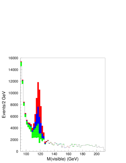
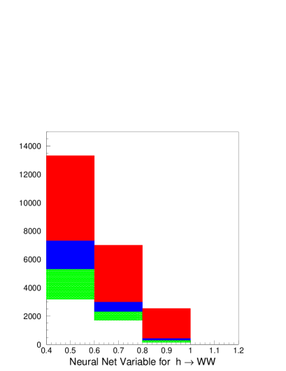
Figure 3: Histograms of $M({\rm visible})$ (left) and the $h\rightarrow WW$ neural net variable (right) following $WW$ selection cuts assuming $M_{h}=120$ GeV. The histograms contain non-Higgs SM background (white), $h\rightarrow W\bar{W}$ (red), $h\rightarrow gg$ (blue), and $h\rightarrow b\bar{b},\ c\bar{c},\ ZZ^{*}$ (green).

Table 2: Statistical accuracies for the measurement of $\sigma\cdot B_{xx}$ for different Higgs decay modes $h\rightarrow xx$ at $\sqrt{s}=1000$ GeV.

	Higgs Mass (GeV)
	115	120	140	160	200
$\Delta(\sigma\cdot B_{bb})/(\sigma\cdot B_{bb})$	$\pm 0.003$	$\pm 0.004$	$\pm 0.005$	$\pm 0.018$	$\pm 0.090$
$\Delta(\sigma\cdot B_{WW})/(\sigma\cdot B_{WW})$	$\pm 0.021$	$\pm 0.013$	$\pm 0.005$	$\pm 0.004$	$\pm 0.005$
$\Delta(\sigma\cdot B_{gg})/(\sigma\cdot B_{gg})$	$\pm 0.014$	$\pm 0.015$	$\pm 0.025$	$\pm 0.145$
$\Delta(\sigma\cdot B_{\gamma\gamma})/(\sigma\cdot B_{\gamma\gamma})$	$\pm 0.053$	$\pm 0.051$	$\pm 0.059$	$\pm 0.237$
$\Delta(\sigma\cdot B_{ZZ})/(\sigma\cdot B_{ZZ})$					$\pm 0.013$

4 Measurement of Higgs Branching Fractions and the Total Higgs Decay Width

The measurements of $\sigma\cdot B_{xx}$ in Table 2 can be converted into model independent measurements of Higgs branching fractions and the total Higgs decay width if they are combined with measurements of the branching fractions $B_{bb}^{*}$ and $B_{WW}^{*}$ from $\sqrt{s}=350$ GeV:

$$B_{xx} = (\sigma\cdot B_{xx})(\sigma\cdot B_{WW})^{-1}B_{WW}^{*}=(\sigma\cdot B_{xx})(\sigma\cdot B_{bb})^{-1}B_{bb}^{*}$$

$$\Gamma_{tot} \propto (\sigma\cdot B_{bb})(B_{bb}^{*})^{-1}(B_{WW}^{*})^{-1}=(\sigma\cdot B_{bb})^{2}(\sigma\cdot B_{WW})^{-1}(B_{bb}^{*})^{-2}.$$ (6)

The assumed values for the errors on $B_{bb}^{*}$ and $B_{WW}^{*}$ are shown in Table 3. The errors are taken from the TESLA TDR[1] when the branching fractions are small. For large branching fractions, however, it is better to use the direct method[10] for measuring branching fractions because binomial statistics reduce the error by a factor of $\sqrt{1-B_{xx}}$.

Utilizing the relations in Eq.(6) a least squares fit is performed to obtain measurement errors for $B_{bb}$, $B_{WW}$, $B_{gg}$, $B_{\gamma\gamma}$, and $\Gamma_{tot}$ at a fixed value of $M_{h}$. The results are summarized in Table 4. Compared to branching fraction measurements at $\sqrt{s}=350$ GeV[1] the results of Table 4 provide a significant improvement for Higgs decay modes with small branching fractions, such as $B_{bb}$ for $160<M_{h}<200$ GeV, $B_{WW}$ for $115<M_{h}<140$ GeV and $B_{gg}$ and $B_{\gamma\gamma}$ for all Higgs masses.

Table 3: Assumed branching fraction errors for Higgs boson decays to $\ bb\$ and $WW$ from measuements made at $\sqrt{s}=350$ GeV with 500 fb^-1 luminosity.

	Higgs Mass (GeV)
	115	120	140	160	200
$\Delta B_{bb}^{*}/B_{bb}^{*}$	$\pm 0.015$	$\pm 0.017$	$\pm 0.026$	$\pm 0.065$	$\pm 0.340$
$\Delta B_{WW}^{*}/B_{WW}^{*}$	$\pm 0.061$	$\pm 0.051$	$\pm 0.025$	$\pm 0.010$	$\pm 0.025$

Table 4: Relative accuracies for the measurement of Higgs branching fractions and the Higgs boson total decay width obtained by combining results from Tables 2 and 3.

	Higgs Mass (GeV)
	115	120	140	160	200
$\Delta B_{bb}/B_{bb}$	$\pm 0.015$	$\pm 0.016$	$\pm 0.018$	$\pm 0.020$	$\pm 0.090$
$\Delta B_{WW}/B_{WW}$	$\pm 0.024$	$\pm 0.020$	$\pm 0.018$	$\pm 0.010$	$\pm 0.025$
$\Delta B_{gg}/B_{gg}$	$\pm 0.021$	$\pm 0.023$	$\pm 0.035$	$\pm 0.146$
$\Delta B_{\gamma\gamma}/B_{\gamma\gamma}$	$\pm 0.055$	$\pm 0.054$	$\pm 0.062$	$\pm 0.237$
$\Delta\Gamma_{tot}/\Gamma_{tot}$	$\pm 0.035$	$\pm 0.034$	$\pm 0.036$	$\pm 0.020$	$\pm 0.050$

5 Conclusion

The couplings of Higgs bosons in the mass range $115<M_{h}<200$ GeV can continue to be measured as the energy of an $e^{+}e^{-}$ linear collider is upgraded to $\sqrt{s}=1000$ GeV. The Higgs event rate is so large that some of the rarer decay modes that were inaccessible at $\sqrt{s}=350$ GeV can be probed at $\sqrt{s}=1000$ GeV, such as $h\rightarrow b\bar{b}$ for $M_{h}=200$ GeV, and $h\rightarrow gg,\ \gamma\gamma$ for $M_{h}=140$ GeV. The Higgs physics results from $\sqrt{s}=1000$ GeV will help provide a more complete picture of the Higgs boson profile.

References

- [1] J. A. Aguilar-Saavedra et al. Tesla technical design report part iii: Physics at an e+e- linear collider. 2001, hep-ph/0106315.
- [2] M. Battaglia and A. De Roeck. eConf, C010630:E3066, 2001, hep-ph/0111307.
- [3] M. Battaglia and A. De Roeck. 2002, hep-ph/0211207.
- [4] International linear collider technical review committee. second report, 2003. SLAC-R-606.
- [5] W. Kilian. Whizard: Complete simulations for electroweak multi- particle processes. Prepared for 31st International Conference on High Energy Physics (ICHEP 2002), Amsterdam, The Netherlands, 24-31 Jul 2002.
- [6] Torbjorn Sjostrand et al. High-energy-physics event generation with pythia 6.1. Comput. Phys. Commun., 135:238–259, 2001, hep-ph/0010017.
- [7] Thorsten Ohl. Circe version 1.0: Beam spectra for simulating linear collider physics. Comput. Phys. Commun., 101:269–288, 1997, hep-ph/9607454.
- [8] M. Pohl and H. J. Schreiber. Simdet - version 4: A parametric monte carlo for a tesla detector. 2002, hep-ex/0206009.
- [9] (ed. ) Behnke, T., (ed. ) Bertolucci, S., (ed. ) Heuer, R. D., and (ed. ) Settles, R. Tesla: The superconducting electron positron linear collider with an integrated x-ray laser laboratory. technical design report. pt. 4: A detector for tesla. DESY-01-011.
- [10] Jean-Claude Brient. The direct method to measure the higgs branching ratios at the future e+e- linear collider. 2002. LC-PHSM-2002-003.