High-precision QCD at hadron colliders:
electroweak gauge boson rapidity distributions
at NNLO

Abstract:

We compute the rapidity distributions of $W$ and $Z$ bosons produced at the Tevatron and the LHC through next-to-next-to leading order in QCD. Our results demonstrate remarkable stability with respect to variations of the factorization and renormalization scales for all values of rapidity accessible in current and future experiments. These processes are therefore “gold-plated”: current theoretical knowledge yields QCD predictions accurate to better than one percent. These results strengthen the proposal to use $W$ and $Z$ production to determine parton-parton luminosities and constrain parton distribution functions at the LHC. For example, LHC data should easily be able to distinguish the central parton distribution fit obtained by MRST from that obtained by Alekhin.

1 Introduction

Drell-Yan production of lepton pairs through electroweak (EW) gauge bosons at hadron colliders occupies a special place in elementary particle physics. Historically, the Drell-Yan mechanism [1] was the first application of parton model ideas beyond deep inelastic scattering, and was later the route to discovery of the $W$ and $Z$ bosons [2]. Currently, it provides precise determinations of several Standard Model (SM) parameters, and places stringent constraints on many forms of new physics. Studies of $W$ production at the Tevatron lead to determinations of the mass and width of the $W$ boson with precision competitive with LEP2 measurements [3, 4, 5, 6]. The ratio of production cross sections for $W$ and $Z$ bosons, weighted by their leptonic branching fractions, is very accurately predicted in the Standard Model, and has been studied extensively at the Tevatron [7]. The rapidity distribution for produced $Z$ bosons [8], and the charge asymmetry in leptons from $W$ production [9], have also been measured at the Tevatron; both distributions are sensitive to the distribution of partons within the proton. Searches for non-standard contributions to the production rate of lepton pairs with invariant masses larger than $M_{W,Z}$ can be used to detect additional gauge bosons, such as the $Z^{{}^{\prime}}$ states that appear in most extensions of the SM. More generally, these searches constrain possible contact interactions between quarks and leptons arising from new physics at energy scales beyond those currently accessible [10].

With Run II of the Tevatron producing data, and with the LHC scheduled to begin operation shortly, an enormous number of $W$ and $Z$ bosons will soon be collected. This will significantly increase the precision of electroweak measurements, and will dramatically boost the sensitivity of new physics searches. To fully utilize these results, precise theoretical predictions for $W$ and $Z$ cross sections are needed. Current calculations are limited by uncertainties in parton distribution functions, as well as higher-order QCD and EW radiative corrections [11].

Parton distribution functions (PDFs) are determined from a global fit to a variety of data; unfortunately there is no direct experimental information for the combined values of $Q^{2}\,(10^{4}~{}{\rm GeV}^{2})$ and Bjorken $x$ ($10^{-4}$ to $10^{-1}$) that are relevant for electroweak physics at the LHC. PDFs for these parameter values are obtained through perturbative evolution of fits to PDFs at lower values of $Q^{2}$, using the DGLAP equation. The complete results for the DGLAP evolution kernels at next-to-next-to leading order (NNLO) are not yet available. An approximate set of evolution kernels is used instead [12].

There are currently two sets of PDFs extracted with NNLO precision, using these approximate kernels. The MRST set [13] utilizes a broad variety of data; the drawback of this procedure is that the data set includes observables for which NNLO QCD corrections are not known. Alekhin’s PDFs [14] are based on deep-inelastic scattering data only; this data set is somewhat restricted, but higher order QCD corrections can be included consistently [15]. The two PDF sets lead to slightly different (at the few percent level) predictions for the total rate of $W$ and $Z$ production at the Tevatron and the LHC [16, 17]. We take this difference as a rough estimate of the current uncertainties in the PDFs needed for Tevatron and LHC physics; the individual PDF fits now also contain intrinsic uncertainty estimates [14, 16].

The QCD corrections to EW gauge boson production have been studied by several groups. The complete NNLO corrections to the total cross section were computed some time ago [18, 19]. However, the total cross section is not an experimental observable, and significant extrapolations are required to compare this prediction to experiment. Ideally, one would like an event generator, at least at the parton level, which retains the full kinematics of the process and incorporates higher-order radiative corrections. Although there has been some recent progress towards this goal at NNLO [20, 21, 22, 23, 24], its completion will probably not occur for some time.

NLO QCD corrections to more differential quantities in EW gauge boson production, including the vector boson rapidity distribution, were computed in Ref. [25]. A generalization of this result to $W$ and $Z$ production at the Tevatron and the LHC yields NLO corrections of approximately 20% to 50%, and scale variations of a few percent. Since the NLO corrections are rather large, while the residual scale dependence is small, the actual reliability of the NLO results has been somewhat unclear. Even taking the NLO scale variations seriously, it is apparent that our knowledge of higher-order QCD corrections to EW gauge boson production is accurate to at best a few percent.

This few percent precision in our knowledge of both PDFs and radiative corrections must be compared to the needs of the Tevatron and LHC physics programs. The $W$ mass should be measured with a precision of $\pm 30$ MeV during Run II in each Tevatron experiment [26]; this uncertainty will be further decreased to $\pm 15$ MeV at the LHC [27]. Such a measurement strengthens the constraints that the precision EW data imposes on the Higgs mass and on many indirect manifestations of new physics. A precise theoretical prediction for $M_{W}$ requires knowledge of the $W$ transverse momentum spectrum, as well as a good understanding of the relevant PDFs. To calibrate the detector response for the measurement of the $W$ decay products, both the rapidity and $p_{\perp}$ spectra of the $Z$ must also be well understood [26]

At the LHC, many additional measurements will also require theoretical predictions accurate to a percent or better. The extremely large cross section for the Drell-Yan process at the LHC allows measurements of the $Z$ boson rapidity distribution, and of the pseudorapidity distribution of charged leptons originating from $W$ decays, to constrain PDFs at the percent level. In effect, $W$ and $Z$ production can serve as a parton-parton “luminosity monitor” [28]. The inferred parton-parton luminosities can then be used to precisely predict rates for interactions with a similar initial state as Drell-Yan production, such as gauge boson pair production processes. Uncertainties in the overall proton-proton luminosity, which is hard to measure precisely at the LHC, will cancel out in this approach.

It is apparent from the above examples that the Tevatron and LHC physics programs require NNLO calculations for differential distributions in kinematic variables; knowledge of inclusive rates is insufficient. Although the inclusive rates for several processes, including Drell-Yan production of lepton pairs, are known at NNLO in QCD, until very recently no complete calculation of a differential quantity existed at NNLO. Such a calculation is quite challenging technically, and traditional methods for the computation of phase-space integrals cannot handle problems of this complexity. In Ref. [29] we described a powerful new method of performing such calculations, and applied it to Drell-Yan production in fixed target experiments. We present here in detail the computation of the rapidity distributions for Drell-Yan production of lepton pairs through $W$ and $(Z,\gamma^{*})$ exchange at both the Tevatron and the LHC through NNLO in QCD. Although these distributions are still not the fully differential results needed for a Monte Carlo event generator, they allow a large number of the physics issues discussed above to be addressed.

Our method extends the optical theorem to allow the tools developed for multi-loop computations to be applied to the calculation of differential distributions. We represent the rapidity constraint by an effective “propagator.” This propagator is constructed so that when the imaginary part of the forward scattering amplitude is computed using the optical theorem, the “mass-shell” constraint for the “particle” described by this propagator is equivalent to the rapidity constraint in the phase space integration. We then use the methods described in Ref. [30] for computing total cross sections, keeping the fake particle propagator in the loop integrals, and deriving the rapidity distribution as the imaginary part of the forward scattering amplitude. We remark that the rapidity distribution for inclusive production of Higgs bosons at hadron colliders, which in the heavy top quark approximation is known at NLO [31], can be computed at NNLO by precisely the same technique; indeed, all the basic integrals encountered in the two problems are identical.

We find that the NNLO corrections to the $W$ and $Z$ rapidity distributions are small for most values of rapidity. This is consistent with the results found in Ref. [18] for the inclusive cross section. However, the magnitude of the corrections can reach a few percent for certain invariant masses and collision energies, indicating that they are required for the precision desired in experimental analyses. The residual scale dependences of the rapidity distributions are below the percent level for all but the largest physically allowed rapidities. The theoretical uncertainty is therefore dominated by our imprecise knowledge of the PDFs. We study the effect of varying the PDF parameterization; we use several fits provided by both MRST and Alekhin. The different MRST sets yield results for the rapidity distributions that vary by $\approx 1\%$ at the LHC; the Alekhin set gives results that differ from those of MRST by 2–8.5% as the rapidity is varied. The anticipated experimental uncertainties at the LHC are sufficiently small to distinguish between such PDF sets. EW gauge boson production can therefore provide important information about the PDFs at the values of $Q^{2}$ and $x$ relevant for collider experiments. Finally, we study the efficacy of various approximations to the complete NNLO result. We find that the common approximation of including only soft gluon corrections does not accurately reproduce the full result for phenomenologically interesting parameter choices.

Our paper is organized as follows. In Section II we introduce our notation. We discuss our method of calculation in detail in Section III. We describe the collinear renormalization of the partonic cross section in Section IV. In Section V we present some analytic results for the partonic rapidity distributions. Numerical results for the $W$ and $Z$ rapidity distributions at both the Tevatron and the LHC are given in Section VI. We present our conclusions in Section VII.

2 Notation

We consider the production of electroweak vector bosons $V$ at hadron colliders,

$$h_{1}+h_{2}\to V+X,$$ (1)

where $X$ stands for any number of additional hadrons, or partons in the perturbative calculation. The $\bar{q}_{i}q_{j}V$ coupling at the tree level is described by the interaction vertex

$${\cal V}_{ij}^{\mu}=ig_{V}C_{ij}\gamma^{\mu}\left(v_{i}^{V}+a_{i}^{V}\gamma_{5}\right),$$ (2)

where the indices $i,j$ denote the quark flavors:

$$i,j=\{u,\bar{u},d,\bar{d},\ldots\}.$$ (3)

The matrix $C_{ij}$ is the unity matrix when $V=\gamma,Z$ and is the CKM matrix when $V=W$. Numerical values for the required CKM matrix elements are given in Section 6.

The vector and axial coefficients for up and down type quarks are:

$$v_{u}^{\gamma}=\frac{2}{3},~{}~{}~{}a_{u}^{\gamma}=0,~{}~{}~{}~{}v_{d}^{\gamma}=-\frac{1}{3},~{}~{}~{}a_{d}^{\gamma}=0,$$

$$v_{u}^{Z}=1-\frac{8}{3}\sin^{2}\theta_{W},~{}~{}~{}a_{u}^{Z}=-1,~{}~{}~{}~{}v_{d}^{Z}=-1+\frac{4}{3}\sin^{2}\theta_{W},~{}~{}~{}a_{d}^{Z}=1,$$

$$v_{u}^{W}=v_{d}^{W}=\frac{1}{\sqrt{2}},~{}~{}~{}~{}a_{u}^{W}=a_{d}^{W}=-\frac{1}{\sqrt{2}}.$$ (4)

The rapidity of the vector boson $V$ is defined as

$$Y\equiv\frac{1}{2}\log\left(\frac{E+p_{z}}{E-p_{z}}\right),$$ (5)

where $E$ and $p_{z}$ are respectively the energy and longitudinal momentum of $V$ in the center-of-mass frame of the colliding hadrons. The cross section for the production of the vector boson can be written as the convolution of partonic hard scattering cross sections with hadronic parton distribution functions:

$$\sigma^{V} = \int_{\frac{1}{2}\ln\tau}^{\frac{1}{2}\ln\frac{1}{\tau}}dY{d\sigma^{V}\over dY}\,,$$

$${d\sigma^{V}\over dY} = \sum_{ab}\int_{\sqrt{\tau}e^{Y}}^{1}\int_{\sqrt{\tau}e^{-Y}}^{1}dx_{1}dx_{2}\ f_{a}^{(h_{1})}(x_{1})f_{b}^{(h_{2})}(x_{2})\ \frac{d\sigma^{V}_{ab}}{dY}(x_{1},x_{2}).$$ (6)

Here,

$$\tau=\frac{m_{V}^{2}}{S},$$ (7)

$m_{V}$ is the invariant mass of $V$, and $S=(P_{1}+P_{2})^{2}$ is the square of the center-of-mass energy of the colliding hadrons $h_{1}$ and $h_{2}$, which carry momenta $P_{1}$ and $P_{2}$ respectively.

As we will see in the next Section, it is beneficial to represent the rapidity constraint in a covariant form. To do so, we introduce the variable $u$, where

$$u=\frac{x_{1}}{x_{2}}e^{-2Y}.$$ (8)

In the center-of-mass frame of the two colliding hadrons, it takes the simple Lorentz invariant form

$$u=\frac{p_{V}\cdot p_{1}}{p_{V}\cdot p_{2}}\,,$$ (9)

where $p_{1}=x_{1}P_{1}$ and $p_{2}=x_{2}P_{2}$ are the momenta of the incoming partons, and $p_{V}$ is the momentum of $V$. The partonic center-of-mass energy is $s=(p_{1}+p_{2})^{2}=Sx_{1}x_{2}$. The partonic $u$-distributions are obtained by integrating the partonic matrix elements over the phase space of the final-state particles with a fixed value of $u$:

$$\frac{d\sigma^{V}_{ab}}{du}=\frac{1}{2s}\int d\Pi_{f}\ \overline{\left\|{\cal M}_{ab\rightarrow V+X}\right\|^{2}}\ \delta\left(\frac{p_{V}\cdot p_{1}}{p_{V}\cdot p_{2}}-u\right).$$ (10)

Here, $\overline{\left\|{\cal M}_{ab\rightarrow V+X}\right\|^{2}}$ denotes the square of the scattering amplitude, averaged over spins and colors of the colliding partons.

The allowed values of $u$ are

$$z\leq u\leq\frac{1}{z},$$ (11)

with

$$z=\frac{m_{V}^{2}}{s}=\frac{\tau}{x_{1}x_{2}}$$ (12)

and

$$\tau\leq z\leq 1.$$ (13)

Inverting Eqs. (8) and (12), the arguments $(x_{1},x_{2})$ of $d\sigma_{ab}^{V}/dY$ in Eq. (6) are given by

$$x_{1}={\sqrt{\tau}e^{Y}\over\sqrt{z/u}}\,,\qquad x_{2}={\sqrt{\tau}e^{-Y}\over\sqrt{uz}}\,.$$ (14)

The boundary values of $(z,u)$ are only achieved for special kinematics (see Fig. 1). For $z=1$, $m_{V}^{2}=s$, and there can be no additional partons radiated in the $V$ boson production process; the kinematics is that of the Born-level process $q\bar{q}\to V$. We refer to the limit $z\to 1$ as the soft limit, since any additional partons must carry little energy. The boundary $u=z$ corresponds to production of a $V$ boson along with one or more partons radiated collinear with incoming parton 2, with momentum $(1-z)p_{2}$. That is, inserting $p_{V}=p_{1}+zp_{2}$ into Eq. (9) leads to $u=z$. Similarly, the boundary $u=1/z$ is achieved when the additional partonic radiation is collinear with incoming parton 1. We refer to the limits $u\to z$ and $u\to 1/z$ as collinear limits.

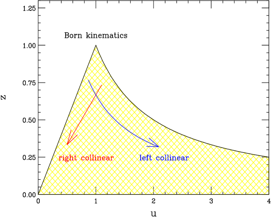
Figure 1: Variables $(z,u)$ used to describe the kinematics of the vector boson rapidity distribution at parton level. The physical region is hatched. The point $u=z=1$ corresponds to no additional radiation, or Born-level kinematics. The left edge, $u=z$, corresponds to radiation of partons collinear with incoming parton 2. The right edge, $u=1/z$, corresponds to radiation collinear with parton 1. The arrows show flows relevant for the convolution integrals encountered in mass factorization (see Section 4).

3 Method

We evaluate the partonic rapidity distributions of Eq. (10) through NNLO in perturbative QCD. The NLO corrections have been previously evaluated in Ref. [25]. However, the calculation of the NNLO corrections is intractable using current techniques. We describe here a new method powerful enough to handle this problem. We express the rapidity constraint as the mass-shell condition of a fake “particle.” This permits the use of the optical theorem to transform the matrix elements into cut forward scattering amplitudes. We can then apply methods developed for multi-loop integration to evaluate these amplitudes. We describe in detail below the required modification of the rapidity constraint, the simplification of the forward scattering amplitude using integration-by-parts reduction algorithms, and the evaluation of the resulting master integrals.

We begin by describing the three distinct contributions that enter at NNLO, to illustrate the difficulties that arise:

• Virtual-Virtual, which contains interferences of diagrams with only the electroweak boson $V$ in the final state;

• Real-Virtual, which contains interferences with the $V$ boson and one additional quark or gluon in the final state;

• Real-Real, which contains interferences of tree-type diagrams with $V$ and two additional partons in the final state.
  

The Virtual-Virtual contribution to the rapidity distribution is identical to its counterpart in the total cross section, which has been computed previously [18]. The new features of the rapidity distribution are the Real-Virtual and Real-Real components, which now have non-trivial kinematic constraints. Until very recently no systematic technique for their evaluation existed; this was the major reason for the lack of progress. However, since the calculation of the inclusive Drell-Yan cross section, our ability to calculate diagrams of the Virtual-Virtual type has progressed greatly. New algorithms for the evaluation of two-loop diagrams of the same [32] and more complicated topologies [33, 34] have been developed. It is now well understood how to organize the evaluation of generic multiloop amplitudes using integration by parts and Lorentz invariance reduction algorithms [34, 35, 36, 37], and how to compute the resulting master integrals using either the Mellin-Barnes [38, 39] or the differential equation method [40, 37]. Our method renders the Real-Virtual and the Real-Real contributions amenable to the same techniques.

3.1 Construction of the modified forward scattering amplitude

We follow the approach introduced in Ref. [30, 41, 31, 29]; we replace all non-trivial phase-space integrations by loop integrations. To accomplish this we represent all delta functions constraining the final-state phase space by

$$\delta(x)=\frac{1}{2\pi i}\left(\frac{1}{x-i0}-\frac{1}{x+i0}\right).$$ (15)

In the evaluation of total cross sections we only have delta functions which put the final-state particles on their mass shell,

$$\int d\Pi_{f}\propto\prod_{f}\int d^{d}p_{f}\ \delta^{+}(p_{f}^{2}-m_{f}^{2}),$$ (16)

where we work in $d=4-2\epsilon$ dimensions, and $\delta^{+}$ includes the positive energy condition $E_{f}>0$. Using Eq. (15), each such delta function becomes a difference of two propagators with opposite prescription for their imaginary part:

$$\delta(p_{f}^{2}-m_{f}^{2})\ \to\ \frac{1}{p_{f}^{2}-m_{f}^{2}-i0}-(c.c.).$$ (17)

When calculating differential quantities, there are additional constraints on the phase space. The distribution constraints can usually be expressed through delta functions with Lorentz-invariant arguments that are polynomial in the momenta of the final-state particles; we then transform them into propagators using Eq. (15).

For the rapidity distribution of the massive boson we substitute

$$\delta\left(\frac{p_{V}\cdot p_{1}}{p_{V}\cdot p_{2}}-u\right)\ \to\ \frac{p_{V}\cdot p_{2}}{p_{V}\cdot\left(p_{1}-up_{2}\right)-i0}-(c.c.).$$ (18)

The above substitution introduces a propagator with a scalar product in the numerator and a denominator linear in the momentum of $V$. However, the multi-loop methods we employ are not sensitive to such irregularities in the form of the propagators; they only require that the propagator of Eq. (18) be polynomial in the momenta. Substituting Eqs.(17) and (18) into Eq. (10), we obtain a forward scattering amplitude with “cut” propagators originating from both the on-shell conditions on the final-state particles and the rapidity constraint. Pictorially, the three different contributions can be represented by diagrams similar to the following ones:

• Virtual-Virtual;
  

• Real-Virtual;
  

• Real-Real.
  

We have associated an additional “rapidity” propagator with the $V$ boson, which we represent by a straight line just to the right of the cut from the usual wavy (cut) $V$ boson propagator. In the above diagrams, cut propagators represent differences of two complex conjugate terms, propagators on different sides of the cut have different prescriptions for their imaginary part, and the initial and final states are identical.

The three contributions are now expressed as two-loop amplitudes in which the cuts denote differences of propagators with opposite $i\epsilon$ prescriptions. These cut conditions are accounted for at the very end of the calculation, after using generic multi-loop methods to simplify the two-loop expressions. We generate the diagrams for the forward scattering amplitude using QGRAF [42]. We then apply the Feynman rules, introduce the rapidity “propagator” of Eq. (18), and perform color and Dirac algebra (we use conventional dimensional regularization) using FORM [43]. This generates a large number of integrals with cut propagators which we must evaluate. The evaluation of these integrals is discussed in the next Section. Our treatment of $\gamma_{5}$ in dimensional regularization follows the discussion in Ref. [18], to which we refer the reader for further details.

3.2 Reduction to Master Integrals

An essential part of the calculation is the reduction of the integrals to a small set of independent master integrals using linear algebraic relations among them. This procedure is routinely applied in computations of virtual amplitudes, such as in the Virtual-Virtual contribution. Our representation of the Real-Virtual and Real-Real terms makes it possible to evaluate them in a similar manner.

We first apply partial fractioning identities to reduce the denominators of the integrands to a linearly independent set. Partial fractioning is always applicable to box diagrams with the introduction of the rapidity constraint. Seven independent scalar products can be formed from the two external momenta $p_{1},p_{2}$ and the two loop momenta $k,l$ (omitting the constant scalar products, $p_{i}\cdot p_{j}$). On the other hand, box topologies with the rapidity propagator have eight terms in the denominator. Thus the eight terms obey one linear relation, which can be used to perform a partial fraction decomposition whenever all terms entering the relation appear as denominators. This step allows us to eliminate one of the uncut propagators in favor of the rapidity propagator. (Whenever a cut propagator or the rapidity propagator does not appear in the denominator of an integral, that integral may be set to zero, by anticipating the delta function constraints.) From this procedure we derive 11 major topologies for the Real-Real contributions, 2 major topologies for the Real-Virtual contributions, and 2 for the Virtual-Virtual contributions. All non-box diagrams are sub-topologies of the above set.

We obtain additional recurrence relations using integration-by-parts (IBP) identities [35, 36]. If $k,l$ are the loop-momenta of the two-loop integrals in the forward scattering amplitude, and $p_{1},p_{2}$ are the incoming momenta, we can write 8 IBP identities of the following form for each integral:

$$0=\int d^{d}k\ d^{d}l\ \frac{\partial}{\partial\eta_{\mu}}\ \frac{q^{\mu}}{k^{2}l^{2}\ldots}\,,$$ (19)

with $\eta^{\mu}=k^{\mu},l^{\mu}$ and $q^{\mu}=k^{\mu},l^{\mu},p_{1}^{\mu},p_{2}^{\mu}$. Each integral contains some cut propagators. However, since differentiation with respect to the loop momenta is insensitive to the prescription for the imaginary part of propagators, the application of IBP reduction algorithms and the taking of cuts commute [30]. This fact allows a straightforward derivation of reduction relations for phase-space integrals. Similarly, we can derive Lorentz invariance identities [37] for phase-space integrals; however, for the Drell-Yan rapidity distribution they are not linearly independent of the IBP relations and provide no additional information.

To solve the system of equations formed by the IBP relations we use an algorithm introduced by Laporta [34]. We construct a large system of explicit IBP identities which we then solve using Gauss elimination. This system should include a sufficient number of equations to reduce all the integrals of the forward scattering amplitudes to master integrals. A detailed description of the algorithm can be found in the original paper of Laporta [34]; we have implemented a customized version in MAPLE [44] and FORM [43]. An important simplification of the reduction procedure in the present case is that we can discard all integrals in which the cut propagators, or the rapidity propagator, are eliminated or appear with negative powers [30]. After performing the reductions, we obtain 5 master integrals for the Virtual-Virtual contributions, 5 for the Real-Virtual, and 19 for the Real-Real.

3.3 Master integrals

All Virtual-Virtual master integrals were known prior to this calculation. The only non-trivial one is the crossed-triangle master integral, which was calculated in Ref. [45, 46]. A list of all Virtual-Virtual master integrals can be found in the appendix of  [30].

For the Real-Virtual contributions we find the following master integrals:

where solid lines correspond to massless scalar propagators

$$\begin{picture}(30.0,30.0)(0.0,8.0)\Line(5,10)(28, 10) \end{picture}\quad\to\quad\frac{1}{p^{2}},$$

bold solid lines correspond to massive scalar propagators

$$\begin{picture}(30.0,30.0)(0.0,8.0)\SetWidth{2} \Line(5,10)(28, 10) \end{picture}\quad\to\quad\frac{1}{p^{2}-m_{V}^{2}},$$

and dashed lines denote the rapidity propagator

$$\begin{picture}(30.0,30.0)(0.0,8.0)\DashLine(5,10)(28, 10){1.5} \end{picture}\quad\to\quad\frac{1}{p_{V}\cdot\left[p_{1}-up_{2}\right]}.$$

The Real-Virtual master integrals can be evaluated by using Eq. (15) to reinstate the delta-function constraints. We then must perform a one-loop integral and a 2-particle phase-space integral; both are straightforward. The most complicated loop integral is a massless one-loop box diagram with one external leg off-shell, which is known to all orders in $\epsilon$ [47]. The Real-Virtual phase-space integration is simple because the polar angle for the 2 $\to$ 2 process is fixed by the rapidity constraint, leaving only a $(1-2\epsilon)$-dimensional azimuthal angular integration. It is thus straightforward to derive analytic expressions for the Real-Virtual master integrals which are valid to all orders in $\epsilon$.

The Real-Real phase-space master integrals were unknown prior to this calculation. A few can be evaluated directly; for example, the two simplest master integrals,

$$I[0]=\begin{picture}(80.0,60.0)(0.0,30.0)\Line(10,20)(20, 30) \Line(10,40)(20,30) \Line(60,30)(70,40) \Line(60,30)(70,20) \CArc(40,30)(20,180,360) \DashLine(40,55)(40,5){4} \Line(20, 30)(60, 30) \DashCArc(40,30)(20,0,90){1.5} \SetWidth{2} \CArc(40,30)(20,90,180) \end{picture}=\int d^{d}q_{V}d^{d}q_{1}d^{d}q_{2}\delta^{d}(p_{1}+p_{2}-q_{V}-q_{1}-q_{2})\times$$

$$\hskip 56.9055pt\delta^{+}(q_{V}^{2}-m_{V}^{2})\delta^{+}(q_{1}^{2})\delta^{+}(q_{2}^{2})\delta(q_{V}\cdot\left[p_{1}-up_{2}\right])$$ (20)

and

$$I[1]=\begin{picture}(80.0,60.0)(0.0,30.0)\Line(10,20)(20, 30) \Line(10,40)(20,30) \Line(55,30)(65,40) \Line(55,30)(65,20) \CArc(55,12.5)(17.5,90,180) \Text(23.3,20)[90]{${\bf\times}$} \CArc(37.5, 30)(17.5,180,270) \CArc(37.5, 30)(17.5,270,360) \DashLine(46,50)(46,10){4} \DashCArc(37.5, 30)(17.5,0,60){1.5} \SetWidth{2} \CArc(37.5, 30)(17.5,60,180) \end{picture}=\int d^{d}q_{V}d^{d}q_{1}d^{d}q_{2}\delta^{d}(p_{1}+p_{2}-q_{V}-q_{1}-q_{2})\times$$

$$\hskip 56.9055pt(q_{1}+q_{2})^{2}\delta^{+}(q_{V}^{2}-m_{V}^{2})\delta^{+}(q_{1}^{2})\delta^{+}(q_{2}^{2})\delta(q_{V}\cdot\left[p_{1}-up_{2}\right])$$ (21)

have the following hypergeometric integral representation:

$$I[\nu]=\frac{\Omega_{d-2}\Omega_{d-1}s^{\nu-2\epsilon}}{2^{d}(1+u)^{1-2\epsilon}}\frac{(u-z)^{1+\nu-2\epsilon}(1-uz)^{1+\nu-2\epsilon}}{\left[\sqrt{u}(\sqrt{u}+\sqrt{z})(1+\sqrt{uz})\right]^{1+\nu-\epsilon}}{\cal K}_{\nu}(\delta),$$ (22)

with

$$\Omega_{d}={2\pi^{d/2}\over\Gamma(d/2)}\,,$$ (23)

$${\cal K}_{\nu}(\delta)=\int_{0}^{1}d\chi\chi^{\nu}\left[\chi(1-\chi)(1-\chi\delta)\right]^{-\epsilon}\,,$$ (24)

and

$$\delta=\frac{(\sqrt{u}-\sqrt{z})(1-\sqrt{uz})}{(\sqrt{u}+\sqrt{z})(1+\sqrt{uz})}.$$ (25)

Expanding in $\epsilon$, we obtain

$${\cal K}_{0}(\delta) = 1+\epsilon\,\left[3-{\frac{\left(\delta-1\right)\ln\left(1-\delta\right)}{\delta}}\right]+{\epsilon}^{2}\Bigg{[}{\frac{\left(\delta-1\right)\ln^{2}\left(1-\delta\right)}{\delta}}$$ (26)

$$-3\,{\frac{\left(\delta-1\right)\ln\left(1-\delta\right)}{\delta}}+{\frac{\left(\delta-2\right){\rm Li}_{2}\left(\delta\right)}{\delta}}+9-\frac{{\pi}^{2}}{6}\Bigg{]}+{\cal O}(\epsilon^{3}),$$

and

$${\cal K}_{1}(\delta) = \frac{1}{2}+\frac{\epsilon}{2}\,\left[-{\frac{\left(\delta^{2}-1\right)\ln\left(1-\delta\right)}{{\delta}^{2}}}+{\frac{5\,\delta+2}{2\delta}}\right]+\frac{{\epsilon}^{2}}{2}\Bigg{[}{\frac{\left(\delta^{2}-1\right)\ln^{2}\left(1-\delta\right)}{{\delta}^{2}}}$$ (27)

$$-5\,{\frac{\left(\delta^{2}-1\right)\ln\left(1-\delta\right)}{2{\delta}^{2}}}+{\frac{\left({\delta}^{2}-2\right){\rm Li}_{2}\left(\delta\right)}{{\delta}^{2}}}+9\,{\frac{3\,\delta+2}{4\delta}}-\frac{{\pi}^{2}}{6}\Bigg{]}+{\cal O}(\epsilon^{3}).$$

In the expression for the scattering amplitude, some of the master integrals are multiplied by coefficients which become singular at the phase-space boundaries. For example, when the $I[\nu]$ master integrals get multiplied by ${1}/{(u-z)^{2+\nu}}$ or $1/{(1-uz)^{2+\nu}}$, the matrix elements become singular at $u=z$ or $u=1/z$ respectively. These singularities are regulated by the non-integer powers of the $(u-z)$ and $(1-uz)$ prefactors in Eq. (22). Upon integrating over $u$ and $z$, they generate $1/\epsilon$ poles which cancel against the Real-Virtual and Real-Real $1/\epsilon$ singularities. For example,

$$\int_{z}^{1/z}du\ (u-z)^{-1-2\epsilon}=-\frac{1}{2\epsilon}\left(\frac{1-z^{2}}{z}\right)^{-2\epsilon}\,.$$ (28)

Since we are interested in the rapidity distribution, we do not integrate over $u$. We must therefore extract these singularities from the Real-Real master integrals. To do so, we factor out the leading behavior of the integral ${\cal X}_{i}$ in the limits $u\to z$ and $u\to 1/z$, keeping the exact $\epsilon$-dependence:

$${\cal X}_{i}(z,u)=(u-z)^{m-\alpha\epsilon}(1-uz)^{n-\beta\epsilon}{\cal F}_{i}(z,u).$$ (29)

The integers $m,n$ are characteristic to each master integral, while $\alpha=\beta=2$ for all Real-Real phase-space integrals. The functions ${\cal F}_{i}$ are smooth and non-zero at $u=z$ and $u=1/z$, and can be calculated as a series in $\epsilon$. In the non-singular regions of phase space we need only calculate the first few terms in the $\epsilon$ expansion, up to the order where polylogarithms of rank 2 appear. However, at $u=z$ and $u=1/z$ additional $1/\epsilon$ coefficients may be generated, and at $u=z=1$ additional $1/\epsilon^{2}$ poles may appear. These require an $\epsilon$ expansion of ${\cal F}_{i}$ up to a transcendentality of rank 3 or 4. We therefore split the master integrals into four different terms:

$${\cal X}_{i}={\cal X}_{i}^{soft}+{\cal X}_{i}^{coll(z)}+{\cal X}_{i}^{coll(\frac{1}{z})}+{\cal X}_{i}^{hard}.$$ (30)

Here,

$${\cal X}_{i}^{soft}=(u-z)^{m-\alpha\epsilon}(1-uz)^{n-\beta\epsilon}{\cal F}_{i}(1,1)$$ (31)

is potentially singular at the limits $u=z$, $u=1/z$ and $u=z=1$;

$${\cal X}_{i}^{coll(z)}=(u-z)^{m-\alpha\epsilon}(1-z^{2})^{n-\beta\epsilon}\left[{\cal F}_{i}(z,z)-{\cal F}_{i}(1,1)\right]$$ (32)

can only become singular at $u=z$;

$${\cal X}_{i}^{coll(\frac{1}{z})}=\left(\frac{1}{z}-z\right)^{m-\alpha\epsilon}(1-uz)^{n-\beta\epsilon}\left[{\cal F}_{i}(z,1/z)-{\cal F}_{i}(1,1)\right]$$ (33)

can only become singular at $u=1/z$; and

$${\cal X}_{i}^{hard}={\cal X}_{i}-{\cal X}_{i}^{soft}-{\cal X}_{i}^{coll(z)}-{\cal X}_{i}^{coll(\frac{1}{z})}$$ (34)

is smooth in all singular limits. We extract the explicit $1/\epsilon$ terms from the $coll$ and $soft$ terms by replacing the $u$ variable with

$$y=\frac{u-z}{(1-z)(1+u)},$$ (35)

where $0\leq y\leq 1$. We then apply identities of the form

$$x^{-1+\epsilon}=\frac{1}{\epsilon}\delta(x)+\sum_{n}\frac{\epsilon^{n}}{n!}\left[\frac{\ln^{n}x}{x}\right]_{+},$$ (36)

for $x=y,1-y$ and $1-z$. The advantage of using the variable $y$ instead of $u$ is that $y$ separates the singularities at $u=z$ and $u=1/z$, which overlap when $z=1$. [At next-to-leading-order, and for the Real-Virtual 2-particle phase space at NNLO, the variable $y$ is related to the $2\to 2$ partonic center-of-mass scattering angle $\theta^{*}$ by $y=(1+\cos\theta^{*})/2$.]

Although a deeper expansion in $\epsilon$ is required for the master integrals in the collinear and soft regions, the calculation is simplified since in the collinear regions the result has a non-trivial dependence on only the variable $z$; in the soft region, the ${\cal F}_{i}$ have no dependence on either $u$ or $z$. For example, while it is difficult to expand ${\cal K}_{\nu}(\delta)$ to higher orders in $\epsilon$ for generic $\delta$, in the soft region, $\delta\to 0$, it can be computed in terms of Gamma functions in closed form:

$${\cal K}_{\nu}(0)=\frac{\Gamma(1+\nu-\epsilon)\Gamma(1-\epsilon)}{\Gamma(2+\nu-2\epsilon)}.$$ (37)

3.4 The differential equation method

The two Real-Real master integrals of the previous subsection were calculated by deriving a simple hypergeometric integral representation starting from their definition as phase-space integrals. However, this is not practical for most master integrals. In more complicated cases we resort to the method of differential equations. This method was developed for loop integrals [40, 37]; however the representation of Eq. (15) for delta function constraints allows its application to phase-space integrations in a straightforward manner [30]. We consider the following master integral as an example:

$${\cal J}(z,u) = \int d^{d}q_{V}d^{d}q_{1}d^{d}q_{2}\ \delta^{d}(p_{1}+p_{2}-q_{V}-q_{1}-q_{2})\times$$ (38)

$$\delta^{+}(q_{V}^{2}-m_{V}^{2})\delta^{+}(q_{1}^{2})\delta^{+}(q_{2}^{2})\delta(q_{V}\cdot[p_{1}-up_{2}])\frac{1}{(q_{1}+q_{V}-p_{1})^{2}}.$$

After applying the transformation of Eq. (15), this integral becomes

$${\cal J}(z,u) = \int d^{d}k\ d^{d}l\ \left[\frac{1}{k^{2}-m_{V}^{2}}\right]_{c}\left[\frac{1}{(k-l)^{2}}\right]_{c}\times$$ (39)

$$\left[\frac{1}{(l+p_{1}+p_{2})^{2}}\right]_{c}\left[\frac{-1}{k\cdot(p_{1}-up_{2})}\right]_{c}\frac{1}{(l+p_{1})^{2}},$$

where $k=-q_{V}$, $l=-q_{V}-q_{1}$, and we denote

$$\left[\frac{1}{x}\right]_{c}=\frac{1}{2\pi i}\left(\frac{1}{x-i0}-\frac{1}{x+i0}\right).$$ (40)

We can now differentiate ${\cal J}(z,u)$ with respect to $z$ and $u$, obtaining

$$\frac{\partial{\cal J}(z,u)}{\partial z} = \int d^{d}k\ d^{d}l\left[\frac{1}{\left(k^{2}-m_{V}^{2}\right)^{2}}\right]_{c}\left[\frac{1}{(k-l)^{2}}\right]_{c}\times$$ (41)

$$\left[\frac{1}{(l+p_{1}+p_{2})^{2}}\right]_{c}\left[\frac{-1}{k\cdot(p_{1}-up_{2})}\right]_{c}\frac{1}{(l+p_{1})^{2}},$$

$$\frac{\partial{\cal J}(z,u)}{\partial u} = \int d^{d}k\ d^{d}l\left[\frac{1}{k^{2}-m_{V}^{2}}\right]_{c}\left[\frac{1}{(k-l)^{2}}\right]_{c}\times$$ (42)

$$\left[\frac{1}{(l+p_{1}+p_{2})^{2}}\right]_{c}\left[\frac{-1}{\left(k\cdot(p_{1}-up_{2})\right)^{2}}\right]_{c}\frac{k\cdot p_{2}}{(l+p_{1})^{2}}.$$

We have set $s=\left(p_{1}+p_{2}\right)^{2}=1$ in these expressions. Neither integral on the right-hand side of Eqs. (41) and (42) is a master integral. However, using IBP we can reduce them to the master integrals ${\cal J}$, $I[0]$, and $I[1]$, using the reduction algorithm of Section 3.2. We then obtain a system of two partial differential equations which determines the functional dependence of ${\cal J}$ on the two kinematic variables $z,u$:

$$\frac{\partial{\cal J}(z,u)}{\partial z} = \frac{2\epsilon}{u-z}{\cal}J(z,u)+\frac{(1-2\epsilon)u\left[(1+3zu+4z)\epsilon-1-zu-2z\right]}{2\epsilon z(u-z)(1-uz)}I[0](z,u)$$ (43)

$$+\frac{(1-2\epsilon)(2-3\epsilon)u}{2\epsilon z(u-z)(1-uz)}I[1](z,u),$$

$$\frac{\partial{\cal J}(z,u)}{\partial u} = -\frac{2\epsilon}{u-z}{\cal}J(z,u)+\frac{(1-2\epsilon)\left[(7+4z-3zu)\epsilon-3-2z+zu\right]}{2\epsilon(u-z)(1-uz)}I[0](z,u)$$ (44)

$$+\frac{(1-2\epsilon)(2-3\epsilon)}{2\epsilon(u-z)(1-uz)}I[1](z,u).$$

The general solution of Eq. (43) is

$${\cal J}(z,u)=\left[{\Omega_{d-1}\over 2^{d-2}}\right]^{2}(u-z)^{-2\epsilon}\left\{\int^{z}dz_{1}\left(u-z_{1}\right)^{2\epsilon}\beta(z_{1},u)+f(u)+{\cal C}\right\},$$ (45)

where $(\Omega_{d-1}/2^{d-2})^{2}\,\beta(z,u)$ is the inhomogeneous part of the differential equation in Eq. (43). We can evaluate the integral in Eq. (45) as a series in $\epsilon$ after we rewrite $\beta$ using the expressions for $I[\nu]$ from subsection 3.3. We obtain

$${\cal R} = \int^{z}dz_{1}\left(u-z_{1}\right)^{2\epsilon}\beta(z_{1},u)=\frac{A_{1}(z,u)}{\epsilon}+A_{0}(z,u)+{\cal O}(\epsilon),$$ (46)

with

$$A_{1}(z,u)=\frac{1}{2}\left[\ln(r)-\ln(r+t)\right]$$ (47)

and

$$A_{0}(z,u) = -\frac{1}{2}\left[\ln(r)+\ln(2)\right]\ln(1+{r}^{2})+\frac{1}{2}\ln(r)\left[2\ln(r)+\ln(2)-4\right]$$ (48)

$$-\frac{1}{2}\ln(t)\ln(r)+\frac{1}{2}\left[\ln(2)+4-\ln(r)+\ln({r}^{2}+1)\right]\ln(r+t)-\frac{1}{2}\ln^{2}(r+t)$$

$$+\frac{1}{2}\ln(t)\ln(r+t)-{\rm Li_{2}}\left[{\frac{(r+t)r}{{r}^{2}+1}}\right]+\frac{1}{2}{\rm Li_{2}}\left[-{\frac{t}{r}}\right]+\frac{1}{2}{\rm Li_{2}}\left[{\frac{r-t}{r}}\right]$$

$$+{\rm Li_{2}}\left[{\frac{2{r}^{2}}{{r}^{2}+1}}\right]-\frac{1}{2}{\rm Li_{2}}\left[{\frac{r-t}{2r}}\right]-\frac{1}{2}{\rm Li_{2}}\left[{\frac{\left(r-t\right)r}{{r}^{2}+1}}\right].$$

We have introduced the notation $r=\sqrt{u}$ and $t=\sqrt{z}$. Substituting the solution of Eq. (45) into the differential equation of Eq. (44), we derive a differential equation for $f(u)$ which we can again solve order by order in $\epsilon$. We find

$$f(u)=\frac{f_{1}(u)}{\epsilon}+f_{0}(u)+{\cal O}(\epsilon),$$ (49)

with

$$f_{1}(u)=\frac{1}{2}\ln(1+r^{2})-\ln(r)$$ (50)

and

$$f_{0}(u) = {\rm Li_{2}}\left[-{r}^{2}\right]+{\rm Li_{2}}\left[\frac{{r}^{2}+1}{2}\right]-{\rm Li_{2}}\left[{r}^{2}\right]+\frac{1}{4}\ln^{2}({r}^{2}+1)-\ln^{2}(r)+4\ln(r)$$ (51)

$$-\frac{1}{2}\left[\ln({r}^{2}+1)+2\ln(r)\right]\ln(2)+\left[\ln(r)-2\right]\ln({r}^{2}+1).$$

Finally, we must determine the constant of integration ${\cal C}$. In principle, this requires an explicit calculation at a specific kinematic point ${\cal J}(z_{0},u_{0})$. However, in many cases we can extract the constant of integration by comparing to the asymptotic behavior of all rapidity phase-space integrals at $u=z=1$, which is identical to that of the basic master integral $I[0]$:

$$\lim_{z,u\to 1}{\rm PS}(z,u)=c(u-z)^{n-2\epsilon}(1-uz)^{m-2\epsilon}.$$ (52)

The $\epsilon$ power of the $u-z$ and $1-uz$ factors is determined by the number of dimensions, $d=4-2\epsilon$; adding more propagators to the basic master integral $I[0]$ can only alter the integers $n,m$ of the asymptotic scaling. We note that the presence of the constant of integration ${\cal C}$ in Eq. (45) violates the scaling of Eq. (52). We can therefore evaluate ${\cal C}$ by requiring that all the terms in Eq. (45) that violate Eq. (52) in the limit $z\to 1,u\to 1$ cancel. We obtain

$${\cal C}=\frac{1}{4}\left[\ln^{2}2+\frac{\pi^{2}}{2}\right]+{\cal O}(\epsilon).$$ (53)

There are master integrals for which the solution of the homogeneous differential equation gives a scaling at $u=z=1$ which is consistent with Eq. (52) for arbitrary values of the constant ${\cal C}$. For these master integrals, we must determine ${\cal C}$ by performing an explicit evaluation in the vicinity of this kinematic point.

As discussed previously, we often need to calculate master integrals in their soft or collinear limits to higher orders in $\epsilon$. For example, the integral ${\cal J}$ is typically divided by an explicit $(u-z)$ factor in the matrix elements, requiring an $\epsilon$-expansion in its collinear limit $u\to z$ which includes the order $\epsilon$ term. We could extend the outlined calculation of ${\cal J}$ for generic $z,u$ to include the ${\cal O}(\epsilon)$ term and then take the limit $u\to z$. However, this would involve expressing the result for generic $z,u$ through generalized polylogarithms of rank 3 with two variables; taking the $u\to z$ limit would collapse them to rank 3 polylogarithms with only the argument $z$. We can avoid the two-variable rank 3 polylogarithms by solving the differential equations directly in the $u\to z$ limit. We express the $z$-dependent term in the general solution of Eq. (45) in the form

$${\cal R}=-\int_{z}^{u}dz_{1}(u-z_{1})^{2\epsilon}\beta(z_{1},u),$$ (54)

and perform the change of variables

$$z_{1}=z+(u-z)\lambda.$$ (55)

Next we expand the integrand in $u-z$ and keep only the leading term. Only the $coll(z)$ limits of the boundary integrals $I[\nu]$ are required, and as explained above those are known to all orders in $\epsilon$. We can then expand Eq. (54) in $\epsilon$; the resulting integration over $\lambda$ involves polylogarithms with a single argument $z$, and can be performed straightforwardly. The computation of $\lim_{u\to z}f(u)$ proceeds as before, utilizing equivalent expansions in $u-z$. Finally, the constant ${\cal C}$ is determined by matching to the asymptotic behavior, $(u-z)^{-2\epsilon}(1-z^{2})^{-2\epsilon}$.

An important check of our results for the master integrals is provided by integrating them over the rapidity variable $u$. The master integrals also enter the NNLO corrections to the rapidity distribution for Higgs boson production at hadron colliders via gluon-gluon fusion, computed in the heavy top quark approximation. Hence the integrated master integrals can be expressed in terms of the master integrals appearing in the evaluation of the Higgs boson total cross section. We have verified that all rapidity-distribution master integrals are consistent with the results of Ref. [30]. The analytic expressions for the master integrals are too lengthy to present here. They can be obtained from the authors by request.

4 Renormalization and mass factorization

The partonic cross sections of Eq. (6), after combining the real and virtual contributions up to ${\cal O}(\alpha_{s}^{2})$, contain $1/\epsilon^{2}$ and $1/\epsilon$ poles arising from both ultraviolet and initial-state collinear singularities. We remove the UV singularities through renormalization in the $\overline{{\rm MS}}$ scheme, and absorb the initial-state singularities into the PDFs using the $\overline{{\rm MS}}$ factorization scheme. First we expand the cross section in the strong coupling constant,

$$\frac{d\sigma_{ij}}{dY}=\frac{d\hat{\sigma}_{ij}^{(0)}}{dY}+\left(\frac{\alpha_{s}^{\prime}}{\pi}\right)\frac{d\hat{\sigma}_{ij}^{(1)}}{dY}+\left(\frac{\alpha_{s}^{\prime}}{\pi}\right)^{2}\frac{d\hat{\sigma}_{ij}^{(2)}}{dY}+{\cal O}((\alpha_{s}^{\prime})^{3}).$$ (56)

The bare strong coupling $\alpha_{s}^{\prime}$ is related to the running strong coupling constant $\alpha_{s}=\alpha_{s}(\mu)$ in the $\overline{{\rm MS}}$ scheme via

$$\alpha_{s}^{\prime}\left(4\pi\right)^{\epsilon}e^{-\epsilon\gamma}=\alpha_{s}\ \mu^{\epsilon}\ \left[1-\frac{\alpha_{s}}{\pi}\frac{\beta_{0}}{\epsilon}+{\cal O}(\alpha_{s}^{2})\right],$$ (57)

with

$$\beta_{0}=\frac{11}{4}-\frac{1}{6}n_{f}.$$ (58)

Here $n_{f}$ is the number of light quark flavors, and $\mu=\mu_{R}=\mu_{F}$ is the combined renormalization and factorization scale. At the end of the calculation, we restore the dependence on $\mu_{R}$ alone, with the aid of the renormalization group equation. Substituting Eq. (57) into Eq. (56) and collecting with respect to $\alpha_{s}$, gives the coefficients of the renormalized expansion,

$$\frac{d\sigma_{ij}}{dY}=\frac{d\sigma_{ij}^{(0)}}{dY}+\left(\frac{\alpha_{s}}{\pi}\right)\frac{d\sigma_{ij}^{(1)}}{dY}+\left(\frac{\alpha_{s}}{\pi}\right)^{2}\frac{d\sigma_{ij}^{(2)}}{dY}+{\cal O}((\alpha_{s})^{3}),$$ (59)

in terms of the bare ones in Eq. (56).

Similarly, to remove the initial-state singularities, we rewrite the hadronic cross section of Eq. (6) using infrared-finite partonic cross sections:

$$\frac{d\sigma^{V}}{dY}=\sum_{ab}\int_{\sqrt{\tau}e^{Y}}^{1}\int_{\sqrt{\tau}e^{-Y}}^{1}dx_{1}dx_{2}\tilde{f}_{a}^{(h_{1})}(x_{1})\tilde{f}_{b}^{(h_{2})}(x_{2})\frac{d\tilde{\sigma}^{V}_{ab}}{dY}(x_{1},x_{2}).$$ (60)

The renormalized parton distribution functions $\tilde{f}^{(h)}_{a}$ are related to the “bare” ones ${f}^{(h)}_{b}$ by

$$\tilde{f}^{(h)}_{a}={f}^{(h)}_{b}\otimes\Gamma_{ab}.$$ (61)

We have introduced the convolution integral

$$\left(f\otimes g\right)(x)=\int_{0}^{1}dydz\ f(y)g(z)\delta(x-yz),$$ (62)

and we implicitly sum over repeated parton indices. The functions $\Gamma_{ab}$ are given in the $\overline{{\rm MS}}$ scheme by

$$\Gamma_{ab}(x) = \delta_{ab}\delta(1-x)-\frac{\alpha_{s}}{\pi}\frac{P_{ab}^{(0)}(x)}{\epsilon}$$ (63)

$$+\left(\frac{\alpha_{s}}{\pi}\right)^{2}\left\{\frac{1}{2\epsilon^{2}}\left[\left(P_{ac}^{(0)}\otimes P_{cb}^{(0)}\right)(x)+\beta_{0}P_{ab}^{(0)}(x)\right]-\frac{1}{2\epsilon}P_{ab}^{(1)}(x)\right\}+{\cal O}(\alpha_{s}^{3}),$$

where the Altarelli-Parisi kernels $P_{ab}^{(n)}$ can be found in Refs. [48]. Substituting Eq. (61) into Eq. (60) and comparing with Eq. (6) we find

$$\frac{d\sigma_{ab}^{V}}{dY}\left(z,u\right)=\int_{\sqrt{\frac{z}{u}}}^{1}\;dy_{1}\;\int_{\sqrt{uz}}^{1}\;dy_{2}\;\Gamma_{ca}(y_{1})\;\frac{d\tilde{\sigma}_{cd}^{V}}{dY}\left(\frac{z}{y_{1}y_{2}},\frac{y_{1}u}{y_{2}}\right)\;\Gamma_{db}(y_{2}).$$ (64)

The convolution integrals follow contours in the $(z,u)$ plane, as shown in Fig. 1. The $y_{1}$ integration, holding $y_{2}$ fixed, sweeps out a flow such as the one marked “left collinear”; whereas the $y_{2}$ integration sweeps along a “right collinear” line. The lower limits of the integration over the $y_{i}$ correspond to the point $(\tilde{z},\tilde{u})\equiv({z\over y_{1}y_{2}},{y_{1}\over y_{2}}u)$ striking one of the two boundaries, $\tilde{u}=\tilde{z}$ or $\tilde{u}=1/\tilde{z}$. We solve Eq. (64) for the finite partonic cross sections $d\tilde{\sigma}_{ab}/dY$ recursively, order by order in the $\alpha_{s}$ expansion.

At this point it is straightforward to derive the finite partonic cross sections. We outline below the salient features of the calculation. All cross sections referred to in the formulas below are finite; we henceforth drop the superscript tilde when referring to them. We will also drop “$d/dY$” to make the formulas more compact.

• To ${\cal O}\left(\alpha_{s}^{2}\right)$, at least one of the two $\Gamma_{ab}$ factors, or $d\sigma_{ab}/dY$, on the right-hand side of Eq. (64) has a delta function containing the convolution variable. If neither $\Gamma_{ab}$ factor contains a delta function, then only the LO cross section enters, with $\tilde{u}=\tilde{z}=1$. This forces both $y_{1}$ and $y_{2}$ to be set to their lower endpoints, $\sqrt{z/u}$ and $\sqrt{zu}$ respectively, so no integral needs to be done. Apart from this case, the double integral in Eq. (64) reduces to a single integral of one of the following two forms: a “right” convolution,

  $$\left[\sigma_{ab}\otimes P^{(n)}_{bc}\right]\left(z,u\right)=\int_{\sqrt{uz}}^{1}dx\,\sigma_{ab}\left(\frac{z}{x},\frac{u}{x}\right)P^{(n)}_{bc}\left(x\right),$$ (65)

  or a “left” convolution,

  $$\left[P^{(n)}_{ba}\otimes\sigma_{bc}\right]\left(z,u\right)=\int_{\sqrt{\frac{z}{u}}}^{1}dx\,\sigma_{ab}\left(\frac{z}{x},xu\right)P^{(n)}_{bc}\left(x\right).$$ (66)

  Using the behavior of the partonic cross sections under inversion of rapidity, $\sigma_{ab}\left(z,\frac{1}{u}\right)=\sigma_{ba}\left(z,u\right)$, it is simple to show that

  $$\left[\sigma_{ab}\otimes P^{(n)}_{bc}\right]\left(z,\frac{1}{u}\right)=\left[P^{(n)}_{bc}\otimes\sigma_{ba}\right]\left(z,u\right).$$ (67)

  We need only consider right convolutions; we can obtain left convolutions by inverting the variable $u$.

• The convolutions required to obtain a finite NLO cross section are of the form $\sigma_{ab}^{(0)}\otimes P^{(0)}_{bc}$. The LO cross section has the following form:

  $$\sigma_{q\bar{q}}^{(0)}\propto\delta\left(1-z\right)\left\{\delta\left(y\right)+\delta\left(1-y\right)\right\},$$ (68)

  where we have used the variable $y$ defined in Eq. (35). Substituting $\sigma^{(0)}$ into the convolution formula in Eq. (65), we find that the resulting $\delta\left(1-\frac{z}{x}\right)$ removes the integration, leaving only the product of $P^{(0)}_{bc}\left(z\right)$ with the remainder of $\sigma^{(0)}$. We note that this remainder contains either $\delta\left(y\right)$ or $\delta\left(1-y\right)$. To put it another way, in Eq. (65), since $\sigma_{q\bar{q}}^{(0)}(z/x,u/x)$ requires $z/x=u/x=1$, the terms generated all have $u=z$, corresponding to $y=0$. The $\delta\left(1-y\right)$ term only contributes in the limit of Born kinematics, $u=z=1$.

• There are three distinct types of convolutions needed in the NNLO cross section: $\sigma_{ab}^{(0)}\otimes P^{(1)}_{bc}$, $\left[\sigma_{ab}^{(0)}\otimes P^{(0)}_{bc}\right]\otimes P^{(0)}_{cd}$, and $\sigma_{ab}^{(1)}\otimes P^{(0)}_{bc}$. The first of these is simple; as in the NLO cross section, the $\delta\left(1-\frac{z}{x}\right)$ from the Born cross section removes the convolution integral, and all the terms generated have $u=z$. We discuss the remaining cases below in some detail.

  • We solve the second type iteratively. The $\sigma_{ab}^{(0)}\otimes P^{(0)}_{bc}$ piece was already computed to obtain the NLO cross section. It contains either $\delta\left(y\right)$ or $\delta\left(1-y\right)$, as noted above. It may also contain distributions in $1-z$. It is simple to show that when performing the second convolution integral using Eq. (65), $\delta\left(1-y\right)\rightarrow\delta\left(x-\sqrt{uz}\right)$ (and again $u=z$), removing the integration. In the $\delta\left(y\right)$ terms, it is convenient to treat plus distributions as follows: for distributions of $1-z$, we set

    $$\left[\frac{{\rm ln}^{n}\left(1-z\right)}{1-z}\right]_{+}\rightarrow\left(1-z\right)^{-1+\epsilon}\Bigg{|}_{\epsilon^{n}},$$ (69)

    where the vertical bar indicates that we should take the appropriate term in the $\epsilon$ expansion defined in Eq. (36). For distributions of $1-x$ arising from the splitting function, we use

    $$\left[\frac{1}{1-x}\right]_{+}\rightarrow\left(1-x\right)^{-1+a\epsilon}\Bigg{|}_{a^{0}},$$ (70)

    where we now must take the ${\cal O}\left(a^{0}\right)$ term. The most complicated integral we must evaluate, which contains plus distributions in both $1-z$ and $1-x$, becomes

    $$I_{1}=\delta\left(y\right)\int_{z}^{1}dx\,f(z/x)\,\left(1-\frac{z}{x}\right)^{-1+\epsilon}\left(1-x\right)^{-1+a\epsilon},$$ (71)

    where $f(z/x)$ is finite in all kinematic limits and we have used the delta function to simplify the lower limit of integration. Performing the variable change $q=(x-z)/(1-z)$, we obtain

    $$I_{1}=\delta\left(y\right)\int_{0}^{1}dq\,\left[q(1-z)+z\right]^{1-\epsilon}f(z/x[q])\left(1-z\right)^{-1+\epsilon\left(1+a\right)}q^{-1+\epsilon}\left(1-q\right)^{-1+a\epsilon},$$ (72)

    where $x[q]=q(1-z)+z$. We can extract the distributions in $1-z$ by using the expansion in Eq. (36). We must also interpret the $q$ and $1-q$ factors as distributions; we set

    $$q^{-1+\epsilon}=\frac{1}{\epsilon}\delta(q)+\sum_{n}\frac{\epsilon^{n}}{n!}\left[\frac{\ln^{n}q}{q}\right]_{+},$$ (73)

    and utilize a similar expansion for $1-q$. We can now expand the integrand to ${\cal O}\left(a^{0}\epsilon^{n}\right)$. Performing the required integrations, we obtain the result for this convolution in terms of polylogarithms of rank 2 and 3 in the variable $z$.

  • To obtain convolutions of the form $\sigma_{ab}^{(1)}\otimes P^{(0)}_{bc}$, we first return to the form of the NLO cross section before expansion in $\epsilon$, which is

    $$\sigma_{q\bar{q}}^{(1)}\propto y^{-1-\epsilon}\left(1-y\right)^{-1-\epsilon}\left(1-z\right)^{-2-2\epsilon}+\ldots\,\,.$$ (74)

    The ellipsis denotes terms of the form $\sigma_{ab}^{(0)}\otimes P^{(0)}_{bc}$, which are needed for an infrared finite NLO cross section; the convolution of these with $P^{(0)}_{cd}$ has already been discussed, and we ignore them here. We have presented the $q\bar{q}$ cross section; the $qg$ NLO result differs only in the exponents of $y$, $1-y$, and $1-z$ which appear, and the required convolutions proceed similarly to those we now discuss. We again consider the case where the splitting function contains a plus distribution in $1-x$. We rewrite this term using Eq. (70). The integral we must evaluate becomes

    $$I_{2}=\int_{\sqrt{uz}}^{1}dx\,f\left(\frac{z}{x},y_{p}\right)\,y_{p}^{-1-\epsilon}\left(1-y_{p}\right)^{-1-\epsilon}\left(1-\frac{z}{x}\right)^{-2-2\epsilon}\left(1-x\right)^{-1+a\epsilon},$$ (75)

    where

    $$y_{p}=\frac{x\left(u-z\right)}{\left(x-z\right)\left(x+u\right)}$$ (76)

    and $f(\frac{z}{x},y_{p})$ is finite in all kinematic limits. Performing the variable change $q=\left(x-\sqrt{uz}\right)/\left(1-\sqrt{uz}\right)$, the integral becomes

    $$I_{2} = \int_{0}^{1}dq\,f(z,y;x[q])\,\,g(z,y;x[q],\epsilon)\,\,y^{-1-\epsilon}\left(1-y\right)^{-1-\epsilon\left(1-a\right)}\left(1-z\right)^{-1-\epsilon}$$ (77)

    $$\times q^{-1-\epsilon}\left(1-q\right)^{-1+a\epsilon},$$

    where $x[q]=q(1-\sqrt{uz})+\sqrt{uz}$. We have absorbed terms which are finite in all limits into the function $g$. We extract the singularities in $y$, $1-y$, and $1-z$ using the expansion of Eq. (36); we again interpret the $q$ and $1-q$ factors as distributions, and expand them as in Eq. (73). We can now expand the integrand in both $a$ and $\epsilon$. To obtain the contribution to the NNLO cross section, we take the ${\cal O}\left(a^{0}\right)$ term, and expand it in $\epsilon$ up to and including the ${\cal O}\left(\epsilon^{0}\right)$ piece. The resulting integrals are straightforward to evaluate, and again give polylogarithms of ranks 2 and 3. The rank 3 polylogarithms only appear in the $\delta(y)$ terms, and are functions of $z$ only.

After performing both the UV renormalization and the collinear subtractions discussed above, we obtain finite partonic cross sections.

5 Partonic cross sections

The basic quantities we compute, $d^{2}\sigma^{V\to{\rm leptons}}/dM/dY$, include the probability for the vector boson $V$ to decay into a pair of leptons, e.g. $Z\to l^{+}l^{-}$ or $W^{+}\to l^{+}\nu_{l}$, and are differential in both rapidity $Y$ and di-lepton invariant mass $M$. We shall present our results in a format which is normalized properly for virtual photon production, $\gamma^{*}\to l^{+}l^{-}$ (see Eq. (109) below). For $W$ and $Z$ production, as well as for $\gamma$-$Z$ interference in the $l^{+}l^{-}$ channel, we introduce additional normalization factors $N^{V}$, where:

$$N^{\gamma} = 1;$$

$$N^{Z} = \frac{3}{16s_{W}^{2}c_{W}^{2}\alpha_{\rm QED}}\frac{\Gamma_{Z}B^{Z}_{l}}{M_{Z}}\frac{M^{4}}{(M^{2}-M_{Z}^{2})^{2}+\Gamma_{Z}^{2}M_{Z}^{2}};$$

$$N^{\gamma Z} = \frac{v^{\gamma}_{l}v^{Z}_{l}}{8s_{W}^{2}c_{W}^{2}}\frac{M^{2}(M^{2}-M_{Z}^{2})}{(M^{2}-M_{Z}^{2})^{2}+\Gamma_{Z}^{2}M_{Z}^{2}};$$

$$N^{W} = \frac{3}{4s_{W}^{2}\alpha_{\rm QED}}\frac{\Gamma_{W}B^{W}_{l}}{M_{W}}\frac{M^{4}}{(M^{2}-M_{W}^{2})^{2}+\Gamma_{W}^{2}M_{W}^{2}}.$$ (78)

We have used the notations $\Gamma_{Z}$ and $\Gamma_{W}$ for the total widths of the $Z$ and $W$, $M_{Z}$ and $M_{W}$ for their masses, and $B^{Z}_{l}$ and $B^{W}_{l}$ for their branching fractions into leptons. The leptonic vector couplings appearing in $N^{\gamma Z}$ are given by

$$v_{l}^{\gamma}=-1,\qquad v_{l}^{Z}=-1+4s_{W}^{2},$$ (79)

and $s_{W}$ and $c_{W}$ represent the sine and cosine of the weak mixing angle, respectively.

Finally, we require the luminosity functions $L^{V}_{ij}\left(x_{1},x_{2}\right)$ that enter the hadronic rapidity distribution. These functions contain the PDFs for the partons $i,j$, and appropriate combinations of the electroweak couplings to $V$. We follow closely the notation of Ref. [18]. We first introduce the following $2n_{f}\times 2n_{f}$ matrices:

$$C^{ii}_{\gamma,Z}\left(q_{k},q_{l}\right)=C^{ff}_{\gamma,Z}\left(q_{k},q_{l}\right) = \left\{\begin{array}[]{ll}1&\mbox{if $q_{k}=\bar{q}_{l}$}\\ 0&\mbox{otherwise}\end{array}\right.;$$ (82)

$$C^{if}_{\gamma,Z}\left(q_{k},q_{l}\right) = \left\{\begin{array}[]{ll}1&\mbox{if $q_{k}=q_{l}$}\\ 0&\mbox{otherwise}\end{array}\right.;$$ (85)

$$C^{ii}_{W^{\pm}}\left(q_{k},q_{l}\right) = \left\{\begin{array}[]{ll}|V_{q_{k}q_{l}}|^{2}&\mbox{if $e_{q_{k}}+e_{q_{l}}=\pm 1$}\\ 0&\mbox{otherwise}\end{array}\right.;$$ (88)

$$C^{if}_{W^{\pm}}\left(q_{k},q_{l}\right) = \left\{\begin{array}[]{ll}|V_{q_{k}q_{l}}|^{2}&\mbox{if $e_{q_{k}}=\pm 1+e_{q_{l}}$}\\ 0&\mbox{otherwise}\end{array}\right.;$$ (91)

$$C^{ff}_{W^{\pm}}\left(q_{k},q_{l}\right) = \left\{\begin{array}[]{ll}|V_{q_{k}q_{l}}|^{2}&\mbox{if $e_{q_{k}}+e_{q_{l}}=\mp 1$}\\ 0&\mbox{otherwise}\end{array}\right..$$ (94)

Here $q_{k}$ is an element of either of the following $n_{f}$-dimensional vectors: $Q=\left\{u,d,s,c,b\right\}$, $\bar{Q}=\left\{\bar{u},\bar{d},\bar{s},\bar{c},\bar{b}\right\}$. In Eq. (94), $e_{q_{k}}$ denotes the electric charge of the element, and $V_{q_{k}q_{l}}$ indicates the appropriate CKM matrix element. Using these matrices, we can write the luminosity functions as follows:

$$L^{V}_{NS}\left(x_{1},x_{2}\right) = \sum_{i,j\in Q,\bar{Q}}C^{ii}_{V}\left(q_{i},\bar{q}_{j}\right)\left(v^{V,2}_{i}+a^{V,2}_{i}\right)\,q_{i}\left(x_{1}\right)\,\bar{q}_{j}\left(x_{2}\right);$$

$$L^{V}_{B^{2}}\left(x_{1},x_{2}\right) = \sum_{i\in Q,\bar{Q}}\,\sum_{k,l\in Q}C^{ff}_{V}\left(q_{k},\bar{q}_{l}\right)\left(v^{V,2}_{k}+a^{V,2}_{k}\right)\,q_{i}\left(x_{1}\right)\,\bar{q}_{i}\left(x_{2}\right);$$

$$L^{V}_{BC}\left(x_{1},x_{2}\right) = \sum_{i\in Q,\bar{Q}}\,\sum_{k\in Q,\bar{Q}}\left[C^{if}_{V}\left(q_{i},\bar{q}_{k}\right)+C^{if}_{V}\left(\bar{q}_{i},q_{k}\right)\right]\left(v^{V,2}_{i}+a^{V,2}_{i}\right)\,q_{i}\left(x_{1}\right)\,\bar{q}_{i}\left(x_{2}\right);$$

$$L^{V}_{AB,vec}\left(x_{1},x_{2}\right) = \sum_{i\in Q,\bar{Q}}\,\sum_{k\in Q}C^{ff}_{V}\left(q_{k},\bar{q}_{k}\right)v^{V}_{i}v^{V}_{k}\,q_{i}\left(x_{1}\right)\,\bar{q}_{i}\left(x_{2}\right);$$

$$L^{V}_{AB,ax}\left(x_{1},x_{2}\right) = \sum_{i\in Q,\bar{Q}}\,\sum_{k\in Q}C^{ff}_{V}\left(q_{k},\bar{q}_{k}\right)a^{V}_{i}a^{V}_{k}\,q_{i}\left(x_{1}\right)\,\bar{q}_{i}\left(x_{2}\right);$$

$$L^{V}_{qg}\left(x_{1},x_{2}\right) = \sum_{i,j\in Q,\bar{Q}}C^{if}_{V}\left(q_{i},q_{j}\right)\left(v^{V,2}_{i}+a^{V,2}_{i}\right)\,q_{i}\left(x_{1}\right)\,g\left(x_{2}\right);$$

$$L^{V}_{gq}\left(x_{1},x_{2}\right) = L^{V}_{qg}\left(x_{2},x_{1}\right);$$

$$L^{V}_{C^{2}}\left(x_{1},x_{2}\right) = \sum_{i,j\in Q,\bar{Q}}\,\sum_{k\in Q,\bar{Q}}C^{if}_{V}\left(q_{i},q_{k}\right)\left(v^{V,2}_{i}+a^{V,2}_{i}\right)\,q_{i}\left(x_{1}\right)\,q_{j}\left(x_{2}\right);$$

$$L^{V}_{D^{2}}\left(x_{1},x_{2}\right) = \sum_{i,j\in Q,\bar{Q}}\,\sum_{k\in Q,\bar{Q}}C^{if}_{V}\left(q_{j},q_{k}\right)\left(v^{V,2}_{j}+a^{V,2}_{j}\right)\,q_{i}\left(x_{1}\right)\,q_{j}\left(x_{2}\right);$$

$$L^{V}_{CD,vec}\left(x_{1},x_{2}\right) = \sum_{i,j\in Q,\bar{Q}}\,\sum_{k\in Q,\bar{Q}}C^{if}_{V}\left(q_{i},q_{i}\right)v^{V}_{i}v^{V}_{j}\,q_{i}\left(x_{1}\right)\,q_{j}\left(x_{2}\right);$$

$$L^{V}_{CD,ax}\left(x_{1},x_{2}\right) = \sum_{i,j\in Q,\bar{Q}}\,\sum_{k\in Q,\bar{Q}}C^{if}_{V}\left(q_{i},q_{i}\right)a^{V}_{i}a^{V}_{j}\,q_{i}\left(x_{1}\right)\,q_{j}\left(x_{2}\right);$$

$$L^{V}_{CE_{1}}\left(x_{1},x_{2}\right) = \sum_{i,j\in Q,\bar{Q}}C^{if}_{V}\left(q_{i},q_{j}\right)\left(v^{V,2}_{i}+a^{V,2}_{i}\right)\,q_{i}\left(x_{1}\right)\,q_{j}\left(x_{2}\right);$$

$$L^{V}_{CE_{2}}\left(x_{1},x_{2}\right) = L^{V}_{CE_{1}}\left(x_{2},x_{1}\right);$$

$$L^{V}_{CF}\left(x_{1},x_{2}\right) = \sum_{i\in Q,\bar{Q}}\,\sum_{j\in Q,\bar{Q}}C^{if}_{V}\left(q_{i},q_{j}\right)\left(v^{V,2}_{i}+a^{V,2}_{i}\right)\,q_{i}\left(x_{1}\right)\,q_{i}\left(x_{2}\right);$$

$$L^{V}_{gg}\left(x_{1},x_{2}\right) = \sum_{i,j\in Q}C^{ff}_{V}\left(q_{i},\bar{q}_{j}\right)\left(v^{V,2}_{i}+a^{V,2}_{i}\right)\,g\left(x_{1}\right)\,g\left(x_{2}\right).$$ (95)

In this formula, a function such as $q_{i}\left(x_{1}\right)$ denotes the appropriate parton distribution function. The label $V$ takes the values $\gamma$, $Z$, and $W^{\pm}$. The electroweak couplings $v_{i}^{V}$ and $a_{i}^{V}$ are given in Eq. (4). To obtain the $\gamma$-$Z$ interference luminosity functions, we must use $V=\gamma$ and substitute $v^{\gamma,2}_{i}\rightarrow v^{\gamma}_{i}v^{Z}_{i}$, $v^{\gamma}_{i}v^{\gamma}_{j}\rightarrow\frac{1}{2}\left(v^{\gamma}_{i}v^{Z}_{j}+v^{\gamma}_{j}v^{Z}_{i}\right)$.

The final ingredients required are the partonic hard cross sections for the channels corresponding to the luminosity functions (95), $d\sigma_{ij}^{V}/dY(z,u)$ for $ij\in\{NS,B^{2},BC,\ldots,gg\}$. We have obtained analytic expressions for these functions; however, they are quite lengthy, so we refrain from giving them here. A MAPLE file containing the functions is available from the authors by request. They have also been implemented in C++, as part of a numerical program computing the hadronic rapidity distribution. The bulk of the analytical complexity stems from the “hard” region, away from the boundaries, $z<1$ and $z<u<1/z$ (or $0<y<1$).

The hard functions contain polylogarithms of rank 2, $\mathop{\rm Li}\nolimits_{2}(A_{i}(z,u))$, and there are a large number of possible ways the arguments $A_{i}$ can depend on the underlying variables $z,u$. In most cases, the arguments are rational functions of $t=\sqrt{z}$ and $r=\sqrt{u}$, as in the case of the sample integral ${\cal J}(z,u)$ presented in Eqs. (48) and (51). In four cases, though, we have to introduce functions in which the polylogarithmic arguments are significantly more complicated. The four functions of this type, $J_{3}$, $J_{27}$, $J_{21}$ and $J_{2}$, are given by:

$$J_{3}(z,u) = {1\over 1+u}{\rm Re}\biggl{[}-{1\over 4}\ln^{2}(z/u)-{1\over 4}\ln(1+u)\biggl{(}\ln(z/u)+2\ln(1+tr)$$ (96)

$$\hskip 85.35826pt-2\ln\biggl{(}{d_{1}-r-2t(1+u)\over d_{1}-r}\biggr{)}-2\ln\biggl{(}{d_{1}+r+2t(1+u)\over d_{1}+r}\biggr{)}\biggr{)}$$

$$\hskip 28.45274pt+\mathop{\rm Li}\nolimits_{2}\biggl{(}{2t(1+u)\over d_{1}-r}\biggr{)}+\mathop{\rm Li}\nolimits_{2}\biggl{(}{-2t(1+u)\over d_{1}+r}\biggr{)}$$

$$\hskip 28.45274pt-\mathop{\rm Li}\nolimits_{2}\biggl{(}{2z(1+u)\over r(d_{1}-r)}\biggr{)}-\mathop{\rm Li}\nolimits_{2}\biggl{(}{-2z(1+u)\over r(d_{1}+r)}\biggr{)}\biggr{]}\,,$$

where $d_{1}=\sqrt{u+4z(1+u)}$;

$$J_{27}(z,u) = -{1\over 2rd_{1}}{\rm Re}\biggl{[}\ln\biggl{(}{r_{2}-r_{1}+r_{1}r_{2}-3-2u\over r_{2}-r_{1}-r_{1}r_{2}+3+2u}\biggr{)}$$ (97)

$$\hskip 28.45274pt+\ln\biggl{(}{d_{1}-2tr_{1}+r_{1}r-r_{1}d_{1}+2t+2tu+r\over d_{1}-2tr_{1}+r_{1}r+r_{1}d_{1}-2t-2tu-r}\biggr{)}$$

$$\hskip 28.45274pt+3\ln\biggl{(}{(r-d_{1}+2tr_{1})(1+r_{2}-2r_{1})\over(r+d_{1}-2tr_{1})(1-r_{2}+2r_{1})}\biggr{)}\biggr{]}\,,$$

where $r_{1}=\sqrt{1+u}$, $r_{2}=\sqrt{5+4u}$;

$$J_{21}(z,u) = {\rm Re}\Biggl{\{}{i\over z(1+u)x_{1}}\biggl{[}-\ln(ta_{1}^{+})\ln\biggl{(}{a_{1}^{+}-1\over 1-tra_{1}^{+}}\biggr{)}+\ln(ta_{1}^{-})\ln\biggl{(}{a_{1}^{-}-1\over 1-tra_{1}^{-}}\biggr{)}$$ (98)

$$\hskip 28.45274pt-\mathop{\rm Li}\nolimits_{2}(1-a_{1}^{+})+\mathop{\rm Li}\nolimits_{2}(1-tra_{1}^{+})+\mathop{\rm Li}\nolimits_{2}(1-a_{1}^{-})-\mathop{\rm Li}\nolimits_{2}(1-tra_{1}^{-})\biggr{]}\Biggr{\}}$$

$$\hskip 5.69046pt+{(1+z)(1-tr)\over(1-z)^{2}(1+u)r(r+t)}\ln z\ \ln\biggl{(}{1+z\over 2}\biggl{)}\,,$$

where

$$x_{1} = \sqrt{\biggl{(}{2u\over 1+u}\biggr{)}^{2}{1\over z}-1},\qquad z\leq\biggl{(}{2u\over 1+u}\biggr{)}^{2}\,,$$ (99)

$$= i\sqrt{1-\biggl{(}{2u\over 1+u}\biggr{)}^{2}{1\over z}},\qquad z>\biggl{(}{2u\over 1+u}\biggr{)}^{2}\,,$$

$$a_{1}^{\pm}={2u\over z(1+u)(1\pm ix_{1})}\,;$$ (100)

and

$$J_{2}(z,u) = -J_{3}(z,u)+{1\over 1+u}\biggl{\{}-rd_{1}\,\ln\biggl{|}{2+u+rd_{1}\over 2+u-rd_{1}}\biggr{|}\,J_{27}(z,u)$$ (101)

$$\hskip 5.69046pt+{3\over 4}{\rm Re}\biggl{[}l_{1}\ln\biggl{|}{u(u+2)(r_{2}-1)\over(1+u)(2+u-ur_{2})}\biggr{|}-\ln(1+u)\ln\biggl{|}{(2+u-ur_{2})(r+d_{1})\over r(1+r_{2})(2+u-rd_{1})}\biggr{|}$$

$$\hskip 34.14322pt-l_{2}\ln\biggl{(}{r(u+2)(d_{1}-r)\over(1+u)(2+u-rd_{1})}\biggr{)}-{1\over 6}(l_{1}^{2}-l_{2}^{2})$$

$$\hskip 34.14322pt+\mathop{\rm Li}\nolimits_{2}\biggl{(}{-u(u+2)(1+r_{2})\over 2+u-ur_{2}}\biggr{)}-\mathop{\rm Li}\nolimits_{2}\biggl{(}{-r(u+2)(r+d_{1})\over 2+u-rd_{1}}\biggr{)}$$

$$\hskip 34.14322pt-\mathop{\rm Li}\nolimits_{2}\biggl{(}{2+u+rd_{1}\over(1+u)(2+u-rd_{1})}\biggr{)}+\mathop{\rm Li}\nolimits_{2}\biggl{(}{2+u+ur_{2}\over(1+u)(2+u-ur_{2})}\biggr{)}\biggr{]}$$

$$\hskip 5.69046pt+{1\over 2}\Bigl{(}M_{1}(x_{u})-M_{1}(x_{l})\Bigr{)}+{3\over 8}\pi^{2}\,\Theta(u-1)\biggr{\}}\,,$$

where $\Theta(x)$ is the Heaviside function,

$$l_{1} = \ln\biggl{|}{2+u+ur_{2}\over 2+u-ur_{2}}\biggr{|}\,,\qquad l_{2}=\ln\biggl{|}{2+u+rd_{1}\over 2+u-rd_{1}}\biggr{|}\,,$$

$$M_{1}(x) = {\rm Re}\Biggl{[}-\mathop{\rm Li}\nolimits_{2}\biggl{(}{x+x^{+}\over 2x^{+}}\biggr{)}+\mathop{\rm Li}\nolimits_{2}\biggl{(}{x+x^{-}\over 2x^{-}}\biggr{)}-\mathop{\rm Li}\nolimits_{2}\biggl{(}{x^{+}-x\over x^{+}-x^{-}}\biggr{)}+\mathop{\rm Li}\nolimits_{2}\biggl{(}{x+x^{+}\over x^{+}-x^{-}}\biggr{)}$$

$$\hskip 5.69046pt+{1\over 4}\biggl{(}\ln^{2}\biggl{(}{x+x^{+}\over x-x^{+}}\biggr{)}-\ln^{2}\biggl{(}{x+x^{-}\over x-x^{-}}\biggr{)}\biggr{)}-{1\over 2}\biggl{(}\ln^{2}\biggl{(}{x+x^{+}\over 2x^{+}}\biggr{)}-\ln^{2}\biggl{(}{x+x^{-}\over 2x^{-}}\biggr{)}\biggr{)}$$

$$\hskip 5.69046pt+{1\over 2}\ln\biggl{(}{x+x^{+}\over x-x^{+}}\biggr{)}\ln\biggl{(}{(x+x^{-})(x-x^{-})\over(x^{+}-x^{-})^{2}}\biggr{)}\Biggr{]}\,,$$

$$x^{+} = -{2+u-2r_{1}\over u}={1\over x^{-}}\,,\qquad x_{u}=r_{2}+2r_{1},\qquad x_{l}={d_{1}+2\sqrt{z(1+u)}\over r}\,.$$ (102)

After the use of polylogarithmic identities, the set of arguments of the remaining polylogarithms, $\mathop{\rm Li}\nolimits_{2}(A_{i})$, can be reduced, if desired, to

$$A_{i} \in \biggl{\{}-z,z,{1+z\over 2}\,,-r,-u,{1-u\over 1+u}\,,{1-u\over 2}\,,-{t\over r}\,,{t\over r}\,,{r-t\over 2r}\,,-tr,tr,{1-tr\over 2}\,,{1-r\over 1+tr}\,,{r-1\over r+t}\,,$$ (103)

$$\hskip 8.5359pt{1-t\over r+1}\,,{r(1-t)\over r+1}\,,{u-z\over 1+u}\,,{1-uz\over 1+u}\,,{1-tr\over 1+u}\,,{r(r-t)\over 1+u}\,,{u-1\over r(r+t)}\,,{1-u\over 1+tr}\biggr{\}}\,.$$

The arguments of the logarithms that appear, $\ln(B_{i})$, are drawn from a simpler set,

$$B_{i} \in \{z,1-z,1+t,1+z,u,r-1,r+1,1+u,r-t,r+t,1-tr,1+tr\},$$ (104)

but since they can appear in pairs, there are still quite a few terms of the form $\ln(B_{i})\ln(B_{j})$.

As mentioned above, rank 3 polylogarithms of a single variable, $z$, are generated in the collinear regions, $u=z$ ($\delta(y)$ terms) and $u=1/z$ ($\delta(1-y)$ terms). These collinear terms have a similar form to the NNLO total cross section, integrated over rapidity [18, 19]. We can write the functions appearing, $\mathop{\rm Li}\nolimits_{3}(a_{i})$, in terms of

$$a_{i} \in \biggl{\{}z,-z,1-z,-1-z,1-z^{2},{1+z\over 2}\,,{1-z\over 2}\,,{1-z\over 1+z}\,,{2z\over 1+z}\,,$$ (105)

$$\hskip 8.5359pt-{z\over 2}\,,{z\over 2(1+z)}\,,-{1\over 2z}\,,{1\over 2(1+z)}\,,-{1+z\over z}\biggr{\}}.$$

The rank 2 polylogarithms appearing in the collinear terms, $\mathop{\rm Li}\nolimits_{2}(b_{i})$, have arguments

$$b_{i}\in\biggl{\{}z,-z,-1-z,{1+z\over 2}\,,-{z\over 2}\,,-{1\over 2z}\,,-{1+z\over z}\biggr{\}},$$ (106)

while the arguments of the logarithms, $\ln(c_{i})$, are

$$c_{i}\in\{z,1-z,1+z,2+z,1+2z\}.$$ (107)

The hard functions have integrable, logarithmic singularities in the soft limit $z\to 1$ and the collinear limits $u\to z$ and $u\to 1/z$. However, the complexity of the analytical formulas is such that many of the individual terms in the hard functions have much more severe singularities in these limits, e.g. several powers of $1/(1-z)$ as $z\to 1$. These spurious singularities lead to unacceptable roundoff error. For this reason we construct patching functions, which are used instead of the full functions in thin strips near the singular regions. The patching functions are typically constructed by taking the appropriate limits analytically. Fig. 2 shows the regions in the $(z,u)$ plane which have to be patched. In addition to the soft and collinear regions, there are two other types of regions where the singularities are completely unphysical. For $z=[2u/(1+u)]^{2}$, the variable $x_{1}$ in Eq. (99) vanishes, leading to a singularity in functions containing $J_{21}(z,u)$. There is an equivalent singularity at $z=[2/(1+u)]^{2}$ in functions containing $J_{21}(z,1/u)$. In this pair of strips, the true function is smooth enough that an analytic patch is not necessary; instead, when the point $(z,u)$ lies in the strip, we replace its value by the average of two nearby values on either edge of the strip [49]. Finally, the limit $u\to 1$ is singular, as indicated by the presence of $(r-1)$ in the set $B_{i}$ in Eq. (104); there are spurious power-law singularities as well in this limit.

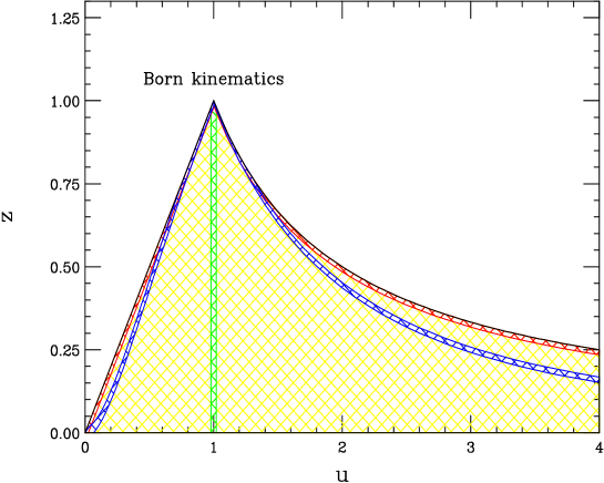
Figure 2: Regions in the $(z,u)$ plane for which the hard functions have to be patched, because of singular behavior. Besides the soft limit $z\to 1$, and the left and right collinear edges, there are spurious singularities as $u\to 1$, and as $z\to[2u/(1+u)]^{2}$ and $z\to[2/(1+u)]^{2}$.

The expansion of the hard functions in a series about $z=1$ can be carried out to very high order, and produces an approximation to the integrand which is free of spurious singularities. Working to order $(1-z)^{25}$ results in an expression whose accuracy is completely adequate for predictions for typical fixed-target kinematics [29] and for $W$ and $Z$ production at the Tevatron. However, for the case of $W$ and $Z$ production at the LHC, the small value of $\tau=M_{V}^{2}/S\approx 4\times 10^{-5}$ means that values of $z\sim 0.01$ are actually relevant in the numerical integration. We have therefore used the exact, unexpanded, representations of the hard functions (plus patches) in order to get sufficient accuracy for the case of the LHC.

6 Numerical results

In this section we present numerical results for the $W$ and $Z$ rapidity distributions at both the Tevatron and the LHC. We use the following parameters: $M_{Z}=91.1876~{}{\rm GeV}$, $\Gamma_{Z}=2.4952~{}{\rm GeV}$, $B^{Z}_{l}=0.03363$, $M_{W}=80.426~{}{\rm GeV}$, $\Gamma_{W}=2.118~{}{\rm GeV}$, and $B^{W}_{l}=0.1082$. We use the $Z$-pole value of $\alpha_{\rm QED}(M_{z})=1/128$ for the fine structure constant, and set ${\rm sin}^{2}{\theta_{W}}=0.23143$, the effective mixing angle measured in $Z$ pole asymmetries at LEP and SLC [50]. We expect that these choices account for the bulk of the factorizable electroweak radiative corrections, which dominate for nearly resonant production of $W$ and $Z$ bosons. A more accurate description would require a consistent accounting of the electroweak corrections [11].

We also need the following values of the CKM matrix elements to compute the $W$ cross section:

$$|V_{ud}|=0.975,~{}~{}~{}|V_{us}|=0.222,~{}~{}~{}|V_{cd}|=0.222,~{}~{}~{}|V_{cs}|=0.974.$$ (108)

The absolute values of the other matrix elements are obtained by requiring unitarity of the CKM matrix. Because the collider center-of-mass energy is large, it is possible in principle to produce top quarks in association with the $W$ or $Z$; however, since these processes can be distinguished experimentally, we exclude them from consideration. We also omit top quarks from the virtual corrections, and set the number of light (massless) quark flavors $n_{f}$ to 5 in all numerical results in this paper. At one loop, the partonic subprocesses $q\bar{q}\rightarrow Zg$ and $qg\rightarrow Zq$ include triangle graphs, weighted by the axial couplings $a_{q}^{Z}$ for the quarks circulating in the loop. For massless quarks, these contributions cancel generation by generation. The effect of a finite top quark mass on the $t-b$ contribution has been studied previously, and found to be negligibly small [18, 51], so we omit it here.

In the previous sections we discussed how the rapidity distributions of electroweak bosons in partonic collisions can be computed. To obtain results for hadronic collisions, we must convolute the partonic differential cross sections with parton distribution functions which describe the probability of finding a parton with a given momentum fraction inside the hadron. The corresponding formula reads:

$$\frac{d^{2}\sigma^{V}}{dMdY}=\frac{4\pi\alpha^{2}_{\rm QED}}{9M^{3}}\sum_{ij}\int dx_{1}dx_{2}\,N^{V}L^{V}_{ij}\left(x_{1},x_{2}\right)\frac{d\sigma_{ij}^{V}}{dY}(x_{1},x_{2}),$$ (109)

where $d\sigma_{ij}^{V}/dY$ is the partonic cross section, $N^{V}$ is the normalization factor for the boson $V$, and $L^{V}_{ij}\left(x_{1},x_{2}\right)$ is the corresponding luminosity function; these were discussed in the previous section. There are three observable cross sections: production of a $W^{+}$; production of a $W^{-}$; and neutral current production of a lepton pair $l^{+}l^{-}$, which receives contributions from both $\gamma$ and $Z$ exchange as well as from $\gamma$-$Z$ interference.

It is convenient to change the integration variables in the above formula and express the integration over $x_{1}$ and $x_{2}$ through the partonic variables $z$ and $y$. Consider the case of negative rapidity $Y$; the results for $Y>0$ can be obtained by substituting $Y\to-Y$ in the formulae below. For $Y<0$, using the relations (8), (12), (14) and (35), the integration over $x_{1}$ and $x_{2}$ in Eq. (109) can be rewritten as:

$$\int dx_{1}dx_{2}\,N^{V}L^{V}_{ij}\left(x_{1},x_{2}\right)\frac{d\sigma_{ij}^{V}}{dY}(x_{1},x_{2})=\int\limits_{\sqrt{\tau}e^{-Y}}^{1}dz\int\limits_{0}^{1}dy\ F_{ij}(z,y)$$

$$\hskip 99.58464pt+\int\limits_{\sqrt{\tau}e^{Y}}^{\sqrt{\tau}e^{-Y}}dz\int\limits_{y_{1}(z)}^{1}dy\ F_{ij}(z,y)+\int\limits_{\tau}^{\sqrt{\tau}e^{Y}}dz\int\limits_{y_{1}(z)}^{y_{2}(z)}dy\ F_{ij}(z,y),$$ (110)

where

$$F_{ij}(z,y)=J(z,y)(1-z)\frac{d\sigma_{ij}^{V}(z,y)}{dY}N^{V}L^{V}_{ij}\left(x_{1},x_{2}\right),$$

$$J(z,y)=\frac{\tau(1+z)}{2z^{2}(1-y(1-z))(z+y(1-z))},$$

$$x_{1}=e^{Y}\sqrt{\frac{\tau}{z}\frac{(z+y(1-z))}{(1-y(1-z))}},\qquad x_{2}=e^{-Y}\sqrt{\frac{\tau}{z}\frac{(1-y(1-z))}{(z+y(1-z))}},$$

$$y_{1}(z)=\frac{\tau e^{-2Y}-z^{2}}{(z+\tau e^{-2Y})(1-z)},\qquad y_{2}(z)=\frac{z(e^{-2Y}-\tau)}{(\tau+e^{-2Y}z)(1-z)}.$$ (111)

This representation is convenient for numerical integration.

We now present results for the $W$ and $Z$ rapidity distributions. For the NNLO calculations, we use the corresponding set of MRST parton distribution functions. The MRST code contains four different sets of PDFs. As mentioned in the inroduction, the complete NNLO evolution kernels needed for a consistent extraction of PDFs at NNLO are not yet known. The MRST program contains both the fastest and slowest possible perturbative evolutions, based upon the known moments of the required DGLAP equations. A third set allows an evolution between these extremes. Finally, a fourth PDF set which seems preferred by large $E_{T}$ jet production at the Tevatron is included. Unless stated otherwise, we use mode 1 of the MRST NNLO PDF code, which corresponds to the intermediate rate of evolution.

For the most part, we present double-differential cross sections, including the decay to leptons,

$${d^{2}\sigma^{V\to{\rm leptons}}\over dMdY}\,.$$ (112)

For the case of on-shell vector bosons, these are evaluated at the resonance peak, $M=M_{W}$ or $M=M_{Z}$. Of course any experiment will integrate over the resonance profile. If this integral is performed in the narrow-resonance approximation, and if the $\gamma$ exchange and $\gamma$-$Z$ interference terms are neglected in the case of the $Z$, the result is

$${d\sigma^{V}\over dY}\ B^{V}_{l}={\pi\over 2}\Gamma_{V}\times{d^{2}\sigma^{V\to{\rm leptons}}\over dMdY}\biggr{|}_{M=M_{V}}\,.$$ (113)

The narrow-resonance conversion factor, $\pi\Gamma_{V}/2$, numerically evaluates to 3.919 GeV for the $Z$ boson, and 3.327 GeV for the $W$. One can further integrate Eq. (113) over the rapidity $Y$ to obtain the theoretical prediction for the “total cross section times branching ratio,” $\sigma^{V}\times B^{V}_{l}$. Our total cross section results for the MRST PDFs, for example, agree with results obtained using the numerical program of Ref. [18], after we omit $b$ quarks from the initial state [52, 53]. (We note that Eqs. (B.13) and (B.16) in the article in Ref. [18] are missing a factor of $T_{\rm f}={1\over 2}$, and the “103” at the end of Eq. (B.11) should have an $x$ multiplying it. Also the normalization of the $W$ cross section in Eqs. (A.3) and (A.11) should be a factor of 2 larger. All these factors are properly included in the numerical program [18].) Our program is also capable of integrating over a range of di-lepton invariant masses, without making the narrow-resonance approximation, and we shall present one such plot below.

We first present, in Fig. 3, the rapidity distribution for a $Z$ boson produced on-shell at the LHC. The LO, NLO, and NNLO results have been included. We have equated the renormalization and factorization scales, and have varied them in the range $M_{Z}/2\leq\mu\leq 2M_{Z}$. At LO the scale variation is large, ranging from 30% at central rapidities to 25% at $Y\approx 3$. This is reduced to $\approx 6\%$ at NLO for all rapidities. At NNLO, the prediction for central rapidities stabilizes dramatically; the scale variation is $\approx 0.6\%$. This increases to 1% at $Y\approx 3$, and 3% at $Y\approx 4$. However, it seems that for $Y\leq 3$, the rapidity values accessible in LHC experiments, the residual scale dependence is no longer a significant theoretical uncertainty when the NNLO corrections are included.

The magnitude of the higher-order corrections exhibits a pattern similar to that of the scale variation. The NLO corrections significantly increase the LO prediction; the LO result is increased by 30% at central rapidities, and by 15% for larger rapidity values. They also change the shape of the distribution, creating a broad peak at central rapidities, as is visible in Fig. 3. The results stabilize completely at NNLO. The NNLO corrections decrease the NLO result by only 1–2%, and do not affect the shape of the distribution.

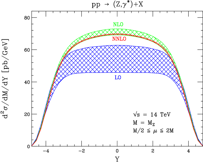
Figure 3: The CMS rapidity distribution of an on-shell $Z$ boson at the LHC. The LO, NLO, and NNLO results have been included. The bands indicate the variation of the renormalization and factorization scales in the range $M_{Z}/2\leq\mu\leq 2M_{Z}$.

For most of the plots in the paper, in order to estimate the uncertainties in the NNLO predictions we shall continue to set $\mu_{F}=\mu_{R}=\mu$ and vary the common scale $\mu$ from $M/2$ to $2M$. However, it is useful to consider a broader range of scale variations, for at least one kinematic configuration. In Fig. 4 we study dependence on $\mu_{F}$ and $\mu_{R}$ in more detail for the case of on-shell $Z$ boson production at the LHC, at the precisely central rapidity point $Y=0$. For each order in perturbation theory (LO, NLO, NNLO), using the MRST PDF sets we plot three curves, corresponding to

• Common variation of the renormalization and factorization scales, $\mu_{F}=\mu_{R}=\mu$, but over a larger range of $\mu$, $M/5<\mu<5M$ (solid curves);

• variation of the factorization scale alone, setting $\mu_{R}=M_{Z}$ (dashed curves);

• variation of the renormalization scale alone, setting $\mu_{F}=M_{Z}$ (dotted curves).

Because the LO result is independent of $\alpha_{s}(\mu_{R})$, the third curve is trivially constant at LO, and the former two LO curves lie on top of each other. We can see from Fig. 4 that the tiny NNLO scale variation in Fig. 3 is not peculiar to the range $M/2<\mu<2M$ used there. Even extending the range to $M/5<\mu<5M$, for a common variation the bandwidth only enlarges from 0.5% to 1.2%. Over this same range, holding $\mu_{F}$ fixed and varying $\mu_{R}$ also produces a quite small range of values, less than 0.5%. The largest variations are found by holding $\mu_{R}$ fixed and varying $\mu_{F}$. These variations are still only of order 0.7% over the range $M/2<\mu<2M$, but rise to of order 5% at the ends of the extended range $M/5<\mu<5M$. The latter are fairly extreme scale choices, however. We believe that the range used in the rest of the paper, $\mu_{F}=\mu_{R}=\mu$ and $M/2<\mu<2M$, provides a good guide to the perturbative uncertainty remaining from the terms beyond NNLO.

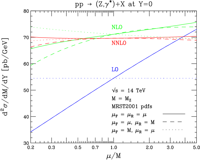
Figure 4: More general variations of the renormalization and factorization scales, for production of an on-shell $Z$ boson at the LHC, at central rapidity $Y=0$. For each order in perturbation theory (LO, NLO, NNLO), three curves are shown. The solid curves depict common variation of the renormalization and factorization scales, $\mu_{F}=\mu_{R}=\mu$, as used in the rest of the paper, but extending the range of variation to $M/5<\mu<5M$. The dashed curves represent variation of the factorization scale alone, holding the renormalization scale fixed at $M$. The dotted curves result from varying the renormalization scale instead, holding the factorization scale fixed at $M$.

In Fig. 5 we present the rapidity distribution for on-shell $Z$ production at Run II of the Tevatron. The scale variation is unnaturally small at LO; it is 3% at central rapidities, and varies from 0.1% to 5% from $Y=1$ to $Y=2$. This occurs because the direction of the scale variation reverses within the range of $\mu$ considered, i.e., $d\sigma_{LO}/d\mu=0$ for a value of $\mu$ which satisifes $M_{Z}/2\leq\mu\leq 2M_{Z}$. This value of $\mu$ depends upon rapidity, leading to scale dependences which vary strongly with $Y$. The scale variation exhibits a more proper behavior at NLO, starting at 3% at central rapidities and increasing to 5–6% at $Y=2.5$. At NNLO the scale dependence is drastically reduced, as at the LHC, and remains below 1% for all relevant rapidity values. The magnitude of the higher-order corrections is slightly larger at the Tevatron than at the LHC. The NLO prediction is higher than the LO result by nearly 45% at central rapidities; this shift decreases to 30% at $Y=1.5$ and to 15% at $Y=2.5$. The NNLO corrections further increase the NLO prediction by 3–5% over the rapidity range $Y\leq 2$.

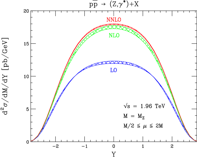
Figure 5: The CMS rapidity distribution of an on-shell $Z$ boson at Run II of the Tevatron. The LO, NLO, and NNLO results have been included. The bands indicate the variation of the renormalization and factorization scales in the range $M_{Z}/2\leq\mu\leq 2M_{Z}$.

This remarkable stability of the rapidity distribution with respect to scale variation cannot be attributed to the smallness of the NNLO QCD corrections to the partonic cross sections. These corrections are the $d\sigma^{(2)}/dY$ terms defined in Eq. (56) (after renormalization and mass factorization), convoluted with the MRST PDFs and with all partonic channels included. We vary the scale in these terms, and normalize this variation to the NLO cross section. We find that the NNLO corrections contribute a scale dependence of $\approx 5\%$ at central rapidities. When we form the complete NNLO cross section, which requires adding these corrections to the convolution of the $d\sigma^{(0)}/dY$ and $d\sigma^{(1)}/dY$ terms of Eq. (56) with NNLO PDFs, the width of this band is decreased to less than 1%. This demonstrates a remarkable interplay between NNLO calculations and parton distribution functions.

The small size of the NNLO corrections is partly due to large cancellations between the various partonic channels. To illustrate this, we present in Fig. 6 the fractional contributions of the various NNLO partonic corrections to the entire NNLO cross section, at Run I of the Tevatron. We include the $qg$ and $q_{i}q_{j}$ channels (the latter includes $qq$ and $q\bar{q}$ inital states); the $gg$ subprocess is numerically unimportant in this process. The magnitude of each order $\alpha_{s}^{2}$ partonic correction, $\delta\sigma_{ij}$, can be 7–8% of the complete NNLO cross section, $\sigma_{\rm NNLO}$, at central rapidities, and can reach 10% of the entire result at larger rapidities. They cancel significantly, however, and their sum is only $\approx 3\%$ of the NNLO result. This cancellation is even larger at LHC energies; in fact, the $q_{i}q_{j}$ and $qg$ channels cancel to such an extent that the $gg$ subprocess becomes an important contribution to the NNLO corrections. This split into partonic components is admittedly not entirely physical, as they are linked by initial-state collinear singularities. However, this degree of cancellation should be rather sensitive to the PDF set chosen. A different choice of PDFs may lead to changes in the cross section that are larger than that found by varying the renormalization and factorization scales.

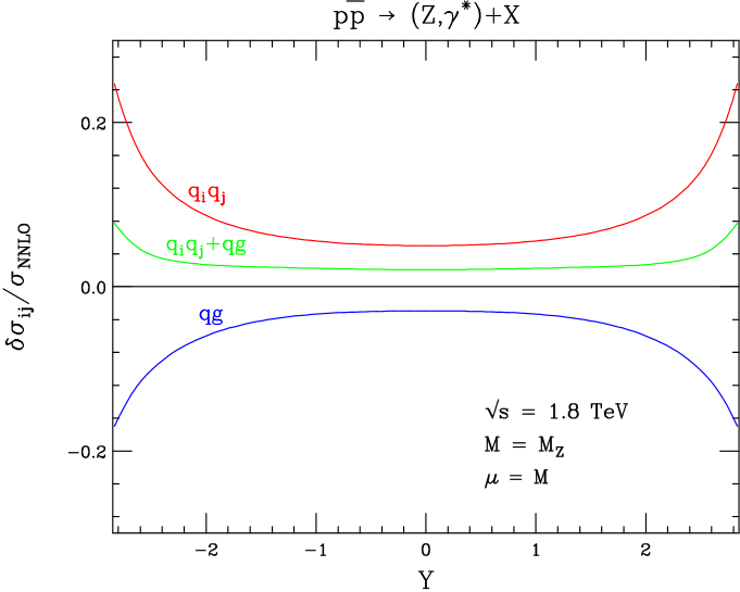
Figure 6: The fractional contribution of the various NNLO partonic channels to the entire NNLO cross section for $Z$ production at Run I of the Tevatron for $\mu=M_{Z}$. $q_{i}q_{j}$ denotes all quark-quark and quark-antiquark channels, while $qg$ indicates the quark-gluon and antiquark-gluon subprocesses. The $gg$ channel is numerically small, and would be consistent with zero on this plot.

To investigate how the choice of PDFs affects the NNLO cross section, we first vary the MRST mode. The choices corresponding to the fast and slow DGLAP evolutions produce negligible shifts in our result, much less than 1% for all rapidities studied, and smaller than the residual scale dependence. (Similar results have been observed at the level of the total cross section [13].) However, the choice of MRST mode 4, which provides a better fit to the Tevatron high-$E_{T}$ jet data, shifts the NNLO $Z$ production cross section significantly. We present in Fig. 7 the rapidity distributions for LHC $Z$ production using these two PDF choices. Both the NLO and NNLO results have been displayed; the scale variations are also included. The two mode choices are indistinguishable at NLO, due to the large residual scale dependence. At NNLO they become quite distinct, and the $\approx 1\%$ discrepancy is potentially visible given projected LHC errors. We note that the difference between the two PDF sets does not just produce a shift in the overall normalization. The mode 4 set slightly increases the number of quarks at $x\sim 0.03$, and decreases the number of gluons more substantially in this $x$ range (to compensate for an even larger increase in $g(x)$ at very large $x$). The $qg$ channel has a negative partonic cross section; thus, paradoxically, decreasing $g(x)$ increases the gluonic contribution to the cross section. The quark and gluon distribution shifts, plus a 2% increase in $\alpha_{s}(M_{Z})$, work in concert to increase the mode 4 predictions, relative to mode 1, for $Z$ production at the LHC at central rapidities, and particularly in the range $1<Y<2$.

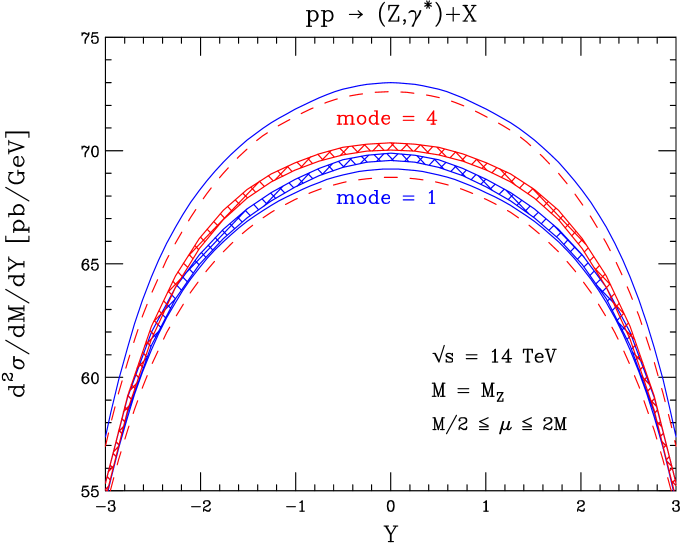
Figure 7: The rapidity distributions for $Z$ production at the LHC for the MRST PDF sets mode 1 and mode 4. The bands indicate the NNLO scale dependences, the solid lines denote the NLO mode 1 scale depedence, and the dashed lines indicate the NLO mode 4 scale variation. The upper lines correspond to the scale choice $\mu=2M$ in the NLO cross sections, while the lower lines indicate $\mu=M/2$.

Another set of PDFs extracted with NNLO precision has been presented by Alekhin [14]. Only deep inelastic scattering data is used in this extraction; the NNLO QCD corrections can therefore be consistently included. The MRST global fits utilize processes for which these corrections are not known. This introduces an additional source of theoretical uncertainty into these parameterizations which is difficult to quantify. We present in Fig. 8 a comparison between the MRST and Alekhin PDF sets for resonant $Z$ production at the LHC. We have included the NNLO scale dependences for the Alekhin set and for the MRST mode 1 and mode 4 sets; the NLO scale dependences for the MRST mode 1 and Alekhin parameterizations are also displayed. The large scale dependences again render all three choices indistinguishable at NLO. However, significant discrepancies appear at NNLO. The difference between the mode 1 and Alekhin sets is 2% at central rapidities; this increases to 4.5% at $Y=2$ and to 8.5% at $Y=3$. The discrepancies in both normalization and shape will be clearly resolvable at the LHC. Although the MRST mode 4 choice is closer to both the shape and normalization of the Alekhin set, the differences still range from 1–8.5% as the rapidity is increased; this will again be observable at the LHC. Electroweak gauge boson production becomes a powerful discriminator between different PDF parameterizations when the NNLO QCD corrections are included.

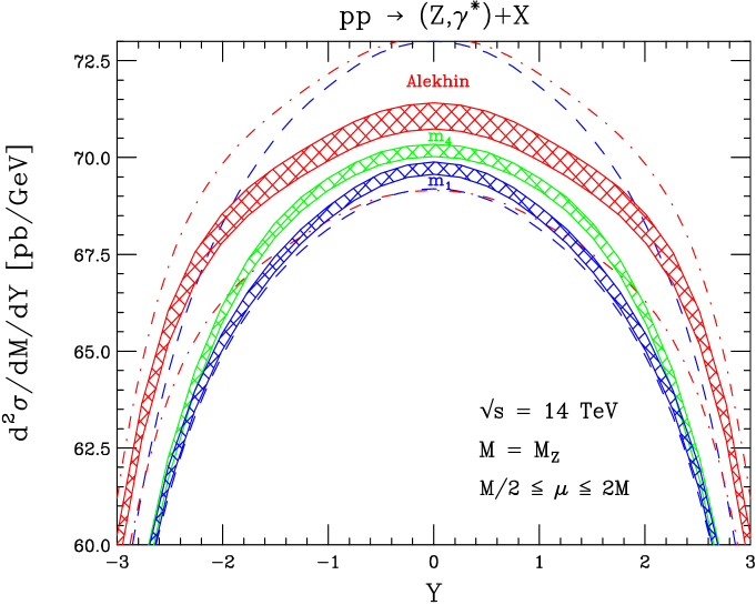
Figure 8: The rapidity distributions for $Z$ production at the LHC for the MRST PDF sets mode 1 and mode 4, and for the Alekhin PDF set. The bands indicate the NNLO scale dependences; ${\rm m}_{1}$ denoted the MRST mode 1 set, while ${\rm m}_{4}$ indicates the MRST mode 4 set. The dashed lines denote the NLO scale dependence for the mode 1 set, and the dot-dashed lines denote the NLO scale dependence for the Alekhin set. The upper lines correspond to the scale choice $\mu=2M$ in the NLO cross sections, while the lower lines indicate $\mu=M/2$.

The di-lepton rapidity distribution for $(Z,\gamma^{*})$ production has been measured by CDF at Run I of the Tevatron, in a mass window around $M_{Z}$, $66<M<116$ GeV [8]. To compare with these data, we numerically integrate over $M$ as well as $z$ and $y$ in Eq. (110). The result is shown in Fig. 9. (The result of doing this $M$ integral in a narrow-resonance approximation, taking into account the finite-mass endpoints, but neglecting photon exchange, is about 2% lower.) The result with the Alekhin PDF set is about 4–5% above the MRST result. Naively, the Alekhin set gives a better fit to the data. However, most of the Alekhin/MRST difference here is in the overall normalization, and there is a 3.9% overall normalization uncertainty in the data (not shown in the error bars) due to the $p\bar{p}$ luminosity uncertainty. Also, electroweak corrections have not yet been included. Hence the two PDF sets probably cannot be distinguished by this Run I data. Instead, it is clear from the figure that, for a given PDF set, the di-lepton rapidity distribution around the $Z$ mass may be used to ‘monitor’ the luminosity at Run II, for which the statistical errors will be significantly smaller than those shown.

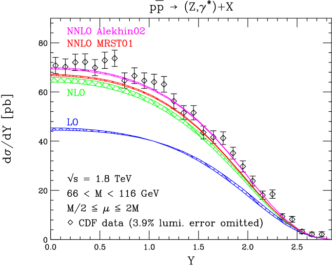
Figure 9: The di-lepton rapidity distribution for $(Z,\gamma^{*})$ production at Run I of the Tevatron, compared with data from CDF [8]. The LO and NLO curves are for the MRST PDF set. The thin NNLO bands are for the MRST (lower) and Alekhin (upper) parameterizations. The bands correspond to varying $M/2\leq\mu\leq 2M$.

We now examine the resonant production of $W$ bosons at Run II of the Tevatron. We present in Fig. 10 the rapidity distribution for $W^{+}$ production; the distribution for the $W^{-}$ can be obtained by substituting $Y\rightarrow-Y$. Both the scale variations and the magnitudes of the higher corrections are similar to those found previously for $Z$ production at the Tevatron. The scale dependence at LO is again unnaturally small, ranging from 3–5%, because $d\sigma_{LO}/d\mu=0$ for values of $\mu$ within the parameter space studied. At NLO the scale variations are between 2% and 3.5%; they decrease to $\approx 0.3$–0.7% at NNLO, depending upon the rapidity chosen. The magnitude of the NLO corrections is large, varying from 45% at central rapidities to $\approx 25\%$ at larger rapidities. The NNLO corrections are also appreciable; they range from 2.5% at $Y=0$ to 4% at $|Y|\approx 2$.

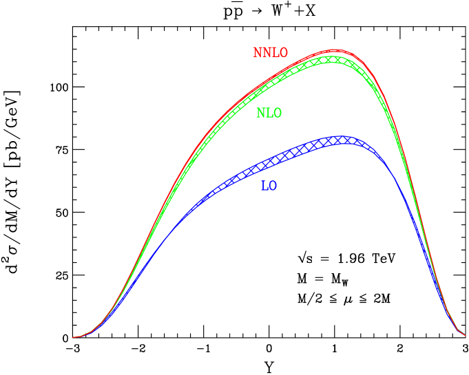
Figure 10: The CMS rapidity distribution of an on-shell $W^{+}$ boson at Run II of the Tevatron. Shown are the LO, NLO, and NNLO results for the MRST PDF sets. The bands indicate the variation of the renormalization and factorization scales in the range $M_{W}/2\leq\mu\leq 2M_{W}$.

Another observable frequently studied at hadron colliders is the $W$ charge asymmetry, defined as

$$A_{W}(Y)=\frac{d\sigma(W^{+})/dY-d\sigma(W^{-})/dY}{d\sigma(W^{+})/dY+d\sigma(W^{-})/dY}.$$ (114)

A simple calculation in the LO approximation reveals that this quantity is sensitive to the $x$ dependence of $u(x)/d(x)$, the ratio of up and down quark distributions in the proton. Although in a realistic experiment only the pseudorapidity of the charged lepton coming from the $W$ decay can be measured, much of the sensitivity to the PDFs remains. Since $A_{W}$ is a ratio of cross sections, it might be expected that it is rather insensitive to QCD corrections. This is indeed the case. At the Tevatron, a $p\bar{p}$ collider, with the assumption of CP invariance, the charge asymmetry is an odd function of $Y$, since it may be written as

$$A_{W}(Y)=\frac{d\sigma(W^{+})/dY-d\sigma(W^{+})/dY|_{Y\to-Y}}{d\sigma(W^{+})/dY+d\sigma(W^{+})/dY|_{Y\to-Y}}=-A_{W}(-Y).$$ (115)

The asymmetry is positive for positive $Y$, corresponding to the $W^{+}$ boson moving in the same direction as the incident proton, because $u(x)$ is larger than $d(x)$ at large $x$. In Fig. 11, we present the LO, NLO, and NNLO predictions for the charge asymmetry at Run II of the Tevatron, together with their scale dependences. The NLO corrections increase the Born level result by 2–4%. The NNLO corrections to the NLO result range from $-2$% at central $W$ rapidities to $+1$% at large rapidities.

The scale variations of $A_{W}(Y)$ are small; to study them, we present in Fig. 12 the scale-dependence bandwidths, defined as

$$B(Y)=\frac{A_{W}(Y,\mu=2M_{W})-A_{W}(Y,\mu=M_{W}/2)}{A_{W}(Y,\mu=M_{W})}.$$ (116)

The scale variation is already below 5% for all rapidities at LO, and is below 1% at NLO. The NNLO prediction is absolutely stable against scale variation, indicating that this observable is potentially a very strong constraint on quark distribution functions. We note that the scale choice $\mu=2M_{Z}$ in the LO asymmetry yields an approximation to the NNLO result which is accurate to 1–2% for essentially all rapidities.

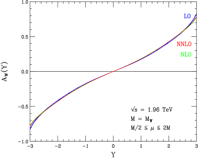
Figure 11: The $W$ charge asymmetry at Run II of the Tevatron. Included are the LO, NLO, and NNLO results. The bands indicate the variation of the renormalization and factorization scales in the range $M_{W}/2\leq\mu\leq 2M_{W}$. As the charge asymmetry is rather insensitive to QCD corrections, the three bands are almost completely degenerate.

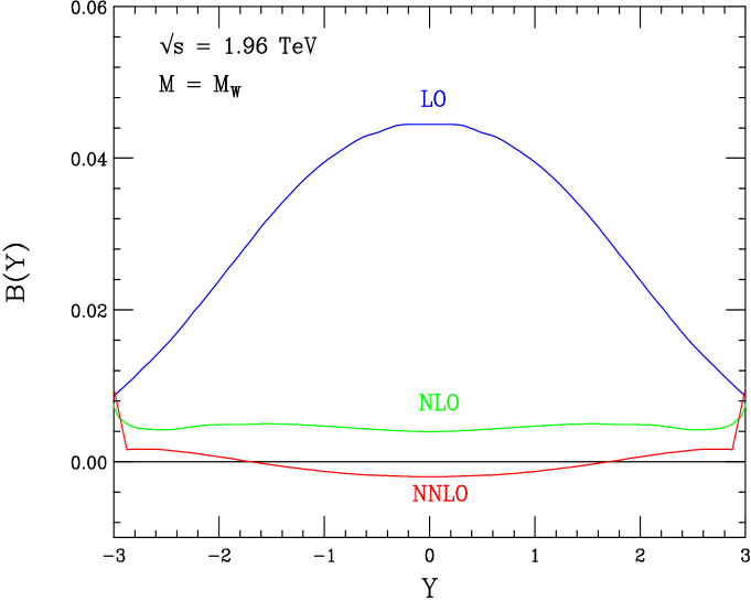
Figure 12: The scale-dependence bandwidths for the $W$ charge asymmetry at the Tevatron. Included are the LO, NLO, and NNLO results.

The NNLO predictions for the rapidity distributions for on-shell $W^{\pm}$ boson production at the LHC are shown in Fig. 13. The distributions are symmetric in $Y$; only the positive half of the rapidity range is shown for $W^{+}$, and the negative half for $W^{-}$. The charge asymmetry is positive for all rapidities, but is particularly striking around $Y=3$. The behavior of the perturbation series is very similar to that discussed previously for $Z$ production at the LHC. Again the NNLO scale-variation bandwidths are extremely narrow for central rapidities, ranging from $\approx 0.6$% for $Y<2$, to 1.5% at $Y=3$, to 3% at $Y=4$.

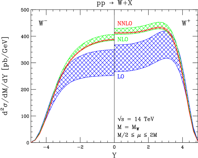
Figure 13: The CMS rapidity distributions for production of an on-shell $W^{-}$ boson (left) and on-shell $W^{+}$ boson (right) at the LHC, at LO, NLO, and NNLO, for the MRST PDF sets. Each distribution is symmetric in $Y$; we only show half the rapidity range in each case. The bands indicate the common variation of the renormalization and factorization scales in the range $M_{W}/2\leq\mu\leq 2M_{W}$.

In addition to the study of resonant production of electroweak gauge bosons, both the Tevatron and the LHC use high-invariant-mass Drell-Yan production of lepton pairs to search for new gauge bosons and lepton-quark contact interactions. Although these are primarily inclusive searches, rapidity cuts are required because of experimental constraints. We therefore examine the NNLO QCD corrections to off-shell $(Z,\gamma^{*})$ production at large invariant masses. We present below the rapidity distribution for $M=250$ GeV $(Z,\gamma^{*})$ production at the LHC in Fig. 14, and for $M=200$ GeV at Run II of the Tevatron in Fig. 15. The scale dependences are significantly smaller for $M=250$ GeV than for resonant $Z$ production at the LHC. The LO scale variation is 12% at central rapidities and 4% at $Y=3$. Both the NLO and NNLO scale variations are much less than 1% for all values of rapidity. The magnitude of the higher-order corrections is much larger, however. The NLO result increases the LO prediction by nearly 35% at central rapidities; this correction decreases to 10% at larger $Y$ values. This discrepancy between the sizes of the scale variations and of the NLO shifts sends a somewhat mixed message regarding the importance of the NNLO corrections. We find that they are small, decreasing the NLO result by less than 0.5% for $Y<1.5$, and increasing it by less than 1% for $1.5<Y<2.8$. The small scale dependence of the NNLO cross section and the stability of the NLO prediction indicate a complete stabilization of the perturbative result for $M=250$ GeV at the LHC.

The results for $M=200$ GeV $(Z,\gamma^{*})$ production at Run II of the Tevatron exhibit both larger scale dependences and more important higher-order corrections. The LO scale variations are similar to those found at the LHC, ranging from 7% at $Y=0$ to $\approx 15\%$ at larger rapidity values. In contrast to the LHC case, the NLO scale dependences remain fairly large, varying from 5% at central rapidities to 14% at $Y=2$. At NNLO, the scale variations are between 1.5% and 4%, again increasing for larger rapidities. The magnitude of the NLO corrections is over 40% at central rapidities, and $\approx 30\%$ at larger $Y$ values. The NNLO corrections further increase the NNLO result by 5–6% throughout the entire rapidity range.

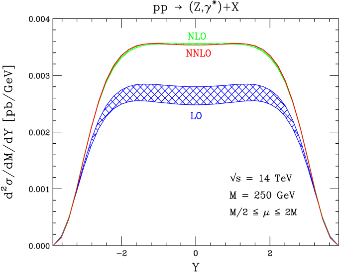
Figure 14: The rapidity distribution for $(Z,\gamma^{*})$ production at the LHC for an invariant mass $M=250$ GeV. The LO, NLO, and NNLO results have been included. The bands indicate the residual scale dependences.

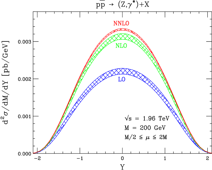
Figure 15: The rapidity distribution for $(Z,\gamma^{*})$ production at Run II of the Tevatron for an invariant mass $M=200$ GeV. The LO, NLO, and NNLO results have been included. The bands indicate the residual scale dependences.

Finally, we study the accuracy of various approximations to the complete NNLO correction to the rapidity distribution. There are three distinct types of terms which appear in the result:

• soft ($s_{z}$): terms which contain either a delta function or a plus distribution in $1-z$. These terms arise from production of the vector boson $V$ close to the partonic threshold, and can be obtained by considering only soft partonic emissions from the $q\bar{q}\rightarrow V$ subprocess.

• collinear ($c_{y}$): terms containing delta functions or plus distributions in either $y$ or $1-y$, but not in $1-z$. These terms result from the emission of radiation collinear to one of the initial partons.

• hard ($h$): terms which have no delta functions or plus distributions. These terms arise from generic scattering events with the emission of hard additional partons in the final state.

There is some potential ambiguity in this separation, due to the presence of Jacobian factors in the integration. We perform the separation in terms of the functions $F_{ij}(z,y)$ appearing in Eq. (110); i.e., including all Jacobian factors resulting from the transformation the variables $(z,y)$. The $s_{z}$ terms can be obtained by using the soft gluon approximation, and it is possible to imagine obtaining the $c_{y}$ contributions from a simplified calculation in which the collinear emission of $V$ is factorized from a hard scattering piece. The hard emissions, however, require a full NNLO computation. Intuitively, we expect the $s_{z}$ terms, which are the simplest to obtain, to dominate for large invariant masses, i.e., as the $z\rightarrow 1$ threshold is approached. We wish to examine whether this contribution, or perhaps the $s_{z}$ and $c_{y}$ terms together, can furnish a reasonable approximation in phenomenologically interesting regions of parameter space.

We present in Figs. 16 and 17 the NNLO corrections to the rapidity distributions for $(Z,\gamma^{*})$ production at the LHC, split into its soft, collinear and hard components, for the invariant masses $M=M_{Z}$ and $M=2$ TeV. The NNLO corrections are the $d\sigma^{(2)}/dY$ terms defined in Eq. (56), convoluted with the MRST PDFs and with all partonic channels included. We present separately the following pieces: the $s_{z}$ term, the $c_{y}$ term, the $h$ term, and the sum of the $h$ and $c_{y}$ pieces, which would integrate to the “hard” (non-soft) part of the total cross section. These terms are normalized to the complete NNLO correction. At $M=M_{Z}$, all components are important. We note that there are large cancellations between the $s_{z}$ term and the remaining pieces. Neither the $s_{z}$ piece nor the sum of the $s_{z}$ and $c_{y}$ terms furnishes a good approximation to the complete result. Generic hard emissions are important; this result is expected, since there is a large amount of phase space available. At $M=2$ TeV, the magnitude of the $s_{z}$ term becomes larger compared to the hard and $c_{y}$ terms, as expected. However, it still does not furnish a good approximation to the entire result for all rapidities; the fact that it does so for central rapidities arises from an accidental cancellation between the hard and $c_{y}$ pieces. We observe similar behavior for Tevatron kinematics. We note that at higher invariant masses, the magnitude of the hard term decreases quickly. The $c_{y}$ term also decreases, but less rapidly. The $s_{z}$ term does not dominate until very large invariant masses are reached.

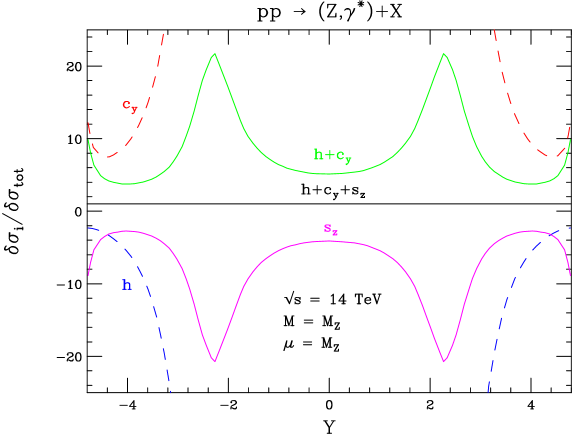
Figure 16: The components of the NNLO corrections to the rapidity distribution for $(Z,\gamma^{*})$ production at the LHC for $M=M_{Z}$. The pieces included are the hard part $h$, $s_{z}$, $c_{y}$, and the sum of the $h$ and $c_{y}$ pieces. The complete NNLO correction $h+c_{y}+s_{z}$ is normalized to unity. We have set $\mu=M$.

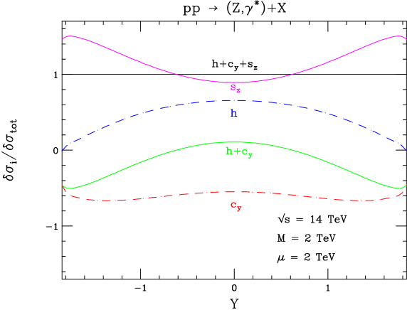
Figure 17: The components of the NNLO corrections to the rapidity distribution for $(Z,\gamma^{*})$ production at the LHC for $M=2$ TeV. The pieces included are the hard part $h$, $s_{z}$, $c_{y}$, and the sum of the $h$ and $c_{y}$ pieces. The complete NNLO correction $h+c_{y}+s_{z}$ is normalized to unity. We have set $\mu=M$.

7 Conclusions

We have presented a calculation of the rapidity distributions for electroweak gauge boson production at hadron colliders through NNLO in QCD. This is the first complete NNLO computation of a differential quantity needed for high-energy hadron collider physics. We have discussed in detail a powerful new technique for calculating differential distributions. This method is completely automated, produces fully analytic results, and treats the various components of a NNLO calculation in a unified manner. Our results will assist in the extraction of parton distribution functions, parton-parton luminosities, electroweak gauge boson information, and other quantities of interest with the accuracy needed for Tevatron and LHC physics.

We have found that the residual scale dependences for resonant $W$ and $Z$ production at both the Tevatron and the LHC are below 1% when the NNLO corrections are included; the rapidity distributions are completely stable against higher-order QCD corrections. Only higher-order electroweak corrections and mixed QCD-electroweak effects remain to be included [11]. These distributions are therefore ideal observables to use to discriminate between different parton distribution function parameterizations. We have studied several different NNLO extractions of parton distribution functions obtained by the MRST group, as well as an NNLO extraction provided by Alekhin. Varying the evolution rate of the approximate NNLO DGLAP kernels in the MRST parameterization yields negligible shifts in our results. However, an MRST PDF set designed to provide a better fit to the Tevatron high-$E_{T}$ jet cross section produces a difference of about $1\%$ in rapidity distributions at the LHC. This difference may be observable, given expected experimental errors.

The deviations induced by instead using Alekhin’s PDF extraction are more striking. Both the normalization and shape of the rapidity distributions obtained with Alekhin’s parameterization differ from those found with the MRST sets; the differences range from 2–8.5% as the rapidity is varied. These differences should be easily resolvable at the LHC, given the expected errors. The MRST parameterizations are derived from global fits to a variety of data, including data from processes for which the NNLO QCD corrections are unknown. We note that the magnitude of the discrepancies between the Alekhin and MRST PDF sets is consistent with the typical size of NNLO QCD corrections. It is conceivable that the inclusion of these corrections into the MRST fit might lessen the observed differences. In fact, the NNLO Alekhin PDF set includes a full error matrix. (Similar uncertainty estimates are available for the MRST set at NLO.) This matrix permits the construction of PDF uncertainty bands for the vector boson rapidity distributions, whereas here we just employed the central PDF values. We defer such a study to future work.

The magnitude of the NNLO corrections to resonant gauge boson production ranges from 1–2% at the LHC to 3–4% at the Tevatron; the corrections for higher invariant mass gauge bosons can reach 5–6% at the Tevatron. These contributions must be included to yield a theoretical calculation accurate to $\approx 1\%$, the projected experimental precision at the LHC. However, the NNLO corrections do not vary strongly with rapidity. The NLO rapidity distribution appears to describe the kinematics quite well. Reweighting the NLO distributions by the inclusive $K$-factor $K^{(2)}=\sigma_{\rm NNLO}/\sigma_{\rm NLO}$ yields an approximation accurate to $\leq 1\%$ for all relevant rapidities. The analogous reweighting of the LO results, by $K^{\rm NNLO}=\sigma_{\rm NNLO}/\sigma_{\rm LO}$, does not furnish a good approximation to the complete result. The excellent accuracy of the NLO reweighting technique for the rapidity distribution suggests that one apply the factor $K^{(2)}$ to output from a hadron-level Monte Carlo program which incorporates the NLO vector-boson production matrix elements, such as MC@NLO 2.2 [54]. This simple procedure should give a good picture of the structure of the hadronic events accompanying the vector bosons, and is likely to approach NNLO precision for sufficiently inclusive observables.

We have also studied the accuracy of approximating the NNLO corrections by partial results. We have found that including only virtual and soft gluon corrections, labeled as $s_{z}$ in the text, does not yield a good approximation for resonant gauge boson production. Only at very large invariant masses do these terms dominate. We estimate that average values of Bjorken $x\geq 0.3-0.4$ must be reached before the $s_{z}$ component accounts for $\approx 80\%$ of the complete NNLO correction for all relevant rapidities. We also note that the $s_{z}$ terms do not accurately predict the shape of the NNLO correction, as is apparent from Figs. 16 and 17.

Finally, we note that with our result for the rapidity distribution, it is possible to obtain almost full control over the kinematics of the electroweak boson, as produced in fixed-order perturbation theory. This is because the NLO QCD corrections to the double differential distribution $d^{2}\sigma/(dYdp_{\perp})$ for electroweak boson production are known [55]. It was assumed in Ref. [55] that $p_{\perp}\neq 0$. It is therefore not possible to perform the integration over $p_{\perp}$ to get $d\sigma/dY$ using the results of Ref. [55] alone. However, the NNLO calculation of the rapidity distribution presented here gives an unambiguous answer for the integral over $p_{\perp}$ at fixed values of rapidity, and can therefore be used as a normalization condition. We write

$$\frac{d^{2}\sigma_{\rm mod}}{dYdp_{\perp}}=\theta(p_{\perp}-p_{\perp}^{\rm cut})\frac{d^{2}\sigma}{dYdp_{\perp}}+\left[\frac{d\sigma}{dY}-\int\limits_{p_{\perp}^{\rm cut}}^{p_{\perp}^{\rm max}}dp_{\perp}\frac{d^{2}\sigma}{dYdp_{\perp}}\right]\theta(p_{\perp}^{\rm cut}-p_{\perp}),$$ (117)

where $d^{2}\sigma/(dYdp_{\perp})$ is the distribution computed in Ref. [55]. Integrating $d^{2}\sigma_{\rm mod}/(dYdp_{\perp})$ over $p_{\perp}$ gives the correct result for the rapidity distribution; however, the “zero $p_{\perp}$” bin extends from $p_{\perp}=0$ to $p_{\perp}=p_{\perp}^{\rm cut}$. Apart from this drawback, Eq. (117) provides a simple way to describe the electroweak boson kinematics at NNLO in QCD.

Our results are an important theoretical input for physics at both the Tevatron and the LHC. We believe the method we have introduced to obtain these results can be used to calculate other phenomenologically interesting observables. We anticipate its application in many other areas of collider physics.

Acknowledgments

We thank S. Alekhin, J. Andersen, F. Gianotti, A. Kotwal, W. Langeveld, M. Peskin, and W.J. Stirling for useful discussions and communications. The work of K.M. is partially supported by the DOE under grant number DE-FG03-94ER-40833 and by the Outstanding Junior Investigator Award DE-FG03-94ER-40833. The work of F.P. is partially supported by the NSF grants P420D3620414350 and P420D3620434350.

References

- [1] S.D. Drell and T.M. Yan, Phys. Rev. Lett. 25, 316 (1970) [Erratum-ibid. 25, 902 (1970)].
-
[2]
G. Arnison et al. [UA1 Collaboration],
Phys. Lett. B 122, 103 (1983);
Phys. Lett. B 126, 398 (1983);
M. Banner et al. [UA2 Collaboration], Phys. Lett. B 122, 476 (1983);
P. Bagnaia et al. [UA2 Collaboration], Phys. Lett. B 129, 130 (1983). - [3] T. Affolder et al. [CDF Collaboration], Phys. Rev. Lett. 85, 3347 (2000) [arXiv:hep-ex/0004017].
- [4] T. Affolder et al. [CDF Collaboration], Phys. Rev. D 64, 052001 (2001) [arXiv:hep-ex/0007044].
- [5] V.M. Abazov et al. [D0 Collaboration], Phys. Rev. D 66, 032008 (2002) [arXiv:hep-ex/0204009].
- [6] V.M. Abazov et al. [D0 Collaboration], Phys. Rev. D 66, 012001 (2002) [arXiv:hep-ex/0204014].
-
[7]
F. Abe et al. [CDF Collaboration],
Phys. Rev. D 52, 2624 (1995);
B. Abbott et al. [D0 Collaboration], Phys. Rev. D 60, 052003 (1999) [arXiv:hep-ex/9901040]; Phys. Rev. D 61, 072001 (2000) [arXiv:hep-ex/9906025]. - [8] T. Affolder et al. [CDF Collaboration], Phys. Rev. D 63, 011101 (2001) [arXiv:hep-ex/0006025].
- [9] F. Abe et al. [CDF Collaboration], Phys. Rev. Lett. 81, 5754 (1998) [arXiv:hep-ex/9809001].
- [10] T. Affolder et al. [CDF Collaboration], Phys. Rev. Lett. 87, 131802 (2001) [arXiv:hep-ex/0106047].
-
[11]
U. Baur, S. Keller and W.K. Sakumoto,
Phys. Rev. D 57, 199 (1998)
[arXiv:hep-ph/9707301];
U. Baur, S. Keller and D. Wackeroth, Phys. Rev. D 59, 013002 (1999) [arXiv:hep-ph/9807417];
U. Baur, O. Brein, W. Hollik, C. Schappacher and D. Wackeroth, Phys. Rev. D 65, 033007 (2002) [arXiv:hep-ph/0108274];
S. Dittmaier and M. Kramer, Phys. Rev. D 65, 073007 (2002) [arXiv:hep-ph/0109062];
U. Baur and D. Wackeroth, Nucl. Phys. Proc. Suppl. 116, 159 (2003) [arXiv:hep-ph/0211089]. - [12] W.L. van Neerven and A. Vogt, Nucl. Phys. B 568, 263 (2000) [arXiv:hep-ph/9907472]; Nucl. Phys. B 588, 345 (2000) [arXiv:hep-ph/0006154]; Phys. Lett. B 490, 111 (2000) [arXiv:hep-ph/0007362].
- [13] A.D. Martin, R.G. Roberts, W.J. Stirling and R.S. Thorne, Phys. Lett. B 531, 216 (2002) [arXiv:hep-ph/0201127].
- [14] S.I. Alekhin, Phys. Rev. D 68, 014002 (2003) [arXiv:hep-ph/0211096].
- [15] E.B. Zijlstra and W.L. van Neerven, Nucl. Phys. B 383, 525 (1992).
- [16] A.D. Martin, R.G. Roberts, W.J. Stirling and R.S. Thorne, arXiv:hep-ph/0308087.
- [17] S.I. Alekhin, arXiv:hep-ph/0307219.
-
[18]
R. Hamberg, W.L. van Neerven and T. Matsuura,
Nucl. Phys. B 359, 343 (1991)
[Erratum-ibid. B 644, 403 (2002)];
http://www.lorentz.leidenuniv.nl/~neerven/ -
[19]
R.V. Harlander and W.B. Kilgore,
Phys. Rev. Lett. 88, 201801 (2002)
[arXiv:hep-ph/0201206];
- [20] D.A. Kosower, Phys. Rev. D 67, 116003 (2003) [arXiv:hep-ph/0212097].
- [21] S. Weinzierl, JHEP 0303, 062 (2003) [arXiv:hep-ph/0302180].
- [22] S. Weinzierl, JHEP 0307, 052 (2003) [arXiv:hep-ph/0306248].
- [23] A. Gehrmann-De Ridder, T. Gehrmann and G. Heinrich, arXiv:hep-ph/0311276.
- [24] C. Anastasiou, K. Melnikov and F. Petriello, arXiv:hep-ph/0311311.
- [25] G. Altarelli, R.K. Ellis and G. Martinelli, Nucl. Phys. B 157, 461 (1979).
- [26] U. Baur, arXiv:hep-ph/0304266.
- [27] G. Azuelos et al., arXiv:hep-ph/0003275.
-
[28]
M. Dittmar, F. Pauss and D. Zürcher,
Phys. Rev. D 56, 7284 (1997)
[arXiv:hep-ex/9705004];
V. A. Khoze, A. D. Martin, R. Orava and M. G. Ryskin, Eur. Phys. J. C 19, 313 (2001) [arXiv:hep-ph/0010163];
W.T. Giele and S.A. Keller, arXiv:hep-ph/0104053. - [29] C. Anastasiou, L. Dixon, K. Melnikov and F. Petriello, Phys. Rev. Lett. 91, 182002 (2003) [arXiv:hep-ph/0306192].
- [30] C. Anastasiou and K. Melnikov, Nucl. Phys. B 646, 220 (2002) [arXiv:hep-ph/0207004].
- [31] C. Anastasiou, L. Dixon and K. Melnikov, Nucl. Phys. Proc. Suppl. 116, 193 (2003) [arXiv:hep-ph/0211141].
- [32] P. A. Baikov and V. A. Smirnov, Phys. Lett. B 477, 367 (2000) [arXiv:hep-ph/0001192].
- [33] C. Anastasiou, T. Gehrmann, C. Oleari, E. Remiddi and J. B. Tausk, Nucl. Phys. B 580, 577 (2000) [arXiv:hep-ph/0003261].
- [34] S. Laporta, Int. J. Mod. Phys. A 15, 5087 (2000) [arXiv:hep-ph/0102033].
- [35] K.G. Chetyrkin and F.V. Tkachov, Nucl. Phys. B 192, 159 (1981).
- [36] F.V. Tkachov, Phys. Lett. B 100, 65 (1981).
- [37] T. Gehrmann and E. Remiddi, Nucl. Phys. B 580, 485 (2000) [arXiv:hep-ph/9912329].
- [38] V.A. Smirnov, Phys. Lett. B 460, 397 (1999) [arXiv:hep-ph/9905323].
- [39] J.B. Tausk, Phys. Lett. B 469, 225 (1999) [arXiv:hep-ph/9909506].
-
[40]
A. V. Kotikov,
Phys. Lett. B 254, 158 (1991);
Z. Bern, L.J. Dixon and D.A. Kosower, Phys. Lett. B 302, 299 (1993) [Erratum-ibid. B 318, 649 (1993)] [arXiv:hep-ph/9212308], Nucl. Phys. B 412, 751 (1994) [arXiv:hep-ph/9306240];
A.V. Kotikov, JINR-E2-93-414;
J. Fleischer, A.V. Kotikov and O.L. Veretin, Phys. Lett. B 417, 163 (1998) [arXiv:hep-ph/9707492]. - [41] C. Anastasiou and K. Melnikov, Phys. Rev. D 67, 037501 (2003) [arXiv:hep-ph/0208115].
- [42] P. Nogueira, J. Comput. Phys. 105, 279 (1993).
- [43] J.A.M. Vermaseren, arXiv:math-ph/0010025.
- [44] MAPLE, http://www.maplesoft.com
- [45] R.J. Gonsalves, Phys. Rev. D 28, 1542 (1983).
- [46] G. Kramer and B. Lampe, J. Math. Phys. 28, 945 (1987).
- [47] C. Anastasiou, E.W.N. Glover and C. Oleari, Nucl. Phys. B 565, 445 (2000) [arXiv:hep-ph/9907523].
-
[48]
G. Altarelli and G. Parisi,
Nucl. Phys. B 126, 298 (1977);
G. Curci, W. Furmanski and R. Petronzio, Nucl. Phys. B 175, 27 (1980);
W. Furmanski and R. Petronzio, Phys. Lett. B 97, 437 (1980);
E.G. Floratos, D.A. Ross and C.T. Sachrajda, Nucl. Phys. B 129, 66 (1977) [Erratum-ibid. B 139, 545 (1978)];
E.G. Floratos, D.A. Ross and C.T. Sachrajda, Nucl. Phys. B 152, 493 (1979). - [49] V. Del Duca, W. Kilgore, C. Oleari, C. Schmidt and D. Zeppenfeld, Nucl. Phys. B 616, 367 (2001) [arXiv:hep-ph/0108030].
- [50] [LEP and SLC Collaborations], arXiv:hep-ex/0212036.
- [51] D.A. Dicus and S.S. Willenbrock, Phys. Rev. D 34, 148 (1986).
- [52] A.D. Martin, R.G. Roberts, W.J. Stirling and R.S. Thorne, Eur. Phys. J. C 23, 73 (2002) [arXiv:hep-ph/0110215].
- [53] W.J. Stirling, private communication.
-
[54]
S. Frixione and B.R. Webber,
JHEP 0206, 029 (2002)
[arXiv:hep-ph/0204244];
S. Frixione, P. Nason and B.R. Webber, JHEP 0308, 007 (2003) [arXiv:hep-ph/0305252];
S. Frixione and B.R. Webber, arXiv:hep-ph/0309186. -
[55]
R.K. Ellis, G. Martinelli and R. Petronzio,
Nucl. Phys. B 211, 106 (1983);
P.B. Arnold and M.H. Reno, Nucl. Phys. B 319, 37 (1989) [Erratum-ibid. B 330, 284 (1990)].