hep-ph/0312250

KEK–TH–902

IPPP/03/41

DCPT/03/82

CERN–TH/2003-162

LTH 613

17 Dec 2003, updated 8 April 2004

Predictions for $g-2$ of the muon and $\alpha_{\rm QED}(M_{Z}^{2})$

K. Hagiwara^a, A.D. Martin^b, Daisuke Nomura^b, and T. Teubner^c,d

^a Theory Group, KEK, Tsukuba, Ibaraki 305-0801, Japan

^b Department of Physics and Institute for Particle Physics Phenomenology,
University of Durham, Durham DH1 3LE, U.K.
^c Theory Division, CERN, CH-1211 Geneva 23, Switzerland
^d Present address: Department of Mathematical Sciences,
University of Liverpool, Liverpool L69 3BX, U.K.

We calculate $(g-2)$ of the muon and the QED coupling $\alpha(M_{Z}^{2})$, by improving the determination of the hadronic vacuum polarization contributions and their uncertainties. We include the recently re-analysed CMD-2 data on $e^{+}e^{-}\to\pi^{+}\pi^{-}$. We carefully combine a wide variety of data for the $e^{+}e^{-}$ production of hadrons, and obtain the optimum form of $R(s)\equiv\sigma_{\rm had}^{0}(s)/\sigma_{\rm pt}(s)$, together with its uncertainty. Our results for the hadronic contributions to $g-2$ of the muon are $a_{\mu}^{\rm had,LO}=(692.4\pm 5.9_{\rm exp}\pm 2.4_{\rm rad})\times 10^{-10}$ and $a_{\mu}^{\rm had,NLO}=(-9.8\pm 0.1_{\rm exp}\pm 0.0_{\rm rad})\times 10^{-10}$, and for the QED coupling $\Delta\alpha^{(5)}_{\rm had}(M_{Z}^{2})=(275.5\pm 1.9_{\rm exp}\pm 1.3_{\rm rad})\times 10^{-4}$. These yield $(g-2)/2=0.00116591763(74)$, which is about $2.4\sigma$ below the present world average measurement, and $\alpha(M_{Z}^{2})^{-1}=128.954\pm 0.031$. We compare our ($g-2$) value with other predictions and, in particular, make a detailed comparison with the latest determination of $(g-2)$ by Davier et al.

1 Introduction

Hadronic vacuum polarization effects play a key role in the prediction of many physical quantities. Here we are concerned with their effect on the prediction of the anomalous magnetic moment of the muon, $a_{\mu}\equiv(g_{\mu}-2)/2$, and on the running of the QED coupling to the $Z$ boson mass. We explain below why it is crucial to predict these two quantities as precisely as possible in order to test the Standard Model and to probe New Physics.

First, we recall that the anomalous magnetic moments of the electron and muon are two of the most accurately measured quantities in particle physics. Indeed the anomalous moment of the electron has been measured to a few parts per billion and is found to be completely described by quantum electrodynamics. This is the most precisely tested agreement between experiment and quantum field theory. On the other hand, since the muon is some 200 times heavier than the electron, its moment is sensitive to small-distance strong and weak interaction effects, and therefore depends on all aspects of the Standard Model. The world average of the existing measurements of the anomalous magnetic moment of the muon is

$$a_{\mu}^{\rm exp}=11659203(8)\times 10^{-10},$$ (1)

which is dominated by the recent value obtained by the Muon $g-2$ collaboration at Brookhaven National Laboratory [1]. Again, the extremely accurate measurement offers a stringent test of theory, but this time of the whole Standard Model. If a statistically significant deviation, no matter how tiny, can be definitively established between the measured value $a_{\mu}^{\rm exp}$ and the Standard Model prediction, then it will herald the existence of new physics beyond the Standard Model. In particular the comparison offers valuable constraints on possible contributions from SUSY particles.

The other quantity, the QED coupling at the $Z$ boson mass, $M_{Z}$, is equally important. It is the least well known of the three parameters (the Fermi constant $G_{\mu}$, $M_{Z}$ and $\alpha(M_{Z}^{2})$), which are usually taken to define the electroweak part of the Standard Model. Its uncertainty is therefore one of the major limiting factors for precision electroweak physics. It limits, for example, the accuracy of the indirect estimate of the Higgs mass in the Standard Model.

The hadronic contributions to $g-2$ of the muon and to the running of $\alpha(s)$ can be calculated from perturbative QCD (pQCD) only for energies well above the heavy flavour thresholds. To calculate the important non-perturbative contributions from the low energy hadronic vacuum polarization insertions in the photon propagator we use the measured total cross section

$$\sigma_{\rm had}^{0}(s)\equiv\sigma_{\rm tot}^{0}(e^{+}e^{-}\to\gamma^{*}\to{\rm hadrons}),$$ (2)

where the 0 superscript is to indicate that we take the bare cross section with no initial state radiative or vacuum polarization corrections, but with final state radiative corrections. Alternatively we may use

$$R(s)=\frac{\sigma_{\rm had}^{0}(s)}{\sigma_{\rm pt}(s)}\,,$$ (3)

where $\sigma_{\rm pt}\equiv 4\pi\alpha^{2}/3s$ with $\alpha=\alpha(0)$. Analyticity and the optical theorem then yield the dispersion relations

$$a_{\mu}^{\rm had,LO}=\left(\frac{\alpha m_{\mu}}{3\pi}\right)^{2}\int_{s_{\rm th}}^{\infty}{\rm d}s\,\frac{R(s)K(s)}{s^{2}}\,,$$ (4)

$$\Delta\alpha_{\rm had}(s)=-\frac{\alpha s}{3\pi}{\rm P}\int_{s_{\rm th}}^{\infty}{\rm d}s^{\prime}\,\frac{R(s^{\prime})}{s^{\prime}(s^{\prime}-s)}\,,$$ (5)

for the hadronic contributions to $a_{\mu}\equiv(g_{\mu}-2)/2$ and $\Delta\alpha(s)=1-\alpha/\alpha(s)$, respectively. The superscript LO on $a_{\mu}$ denotes the leading-order hadronic contribution. There are also sizeable next-to-leading order (NLO) vacuum polarization and so-called “light-by-light” hadronic contributions to $a_{\mu}$, which we will introduce later. The kernel $K(s)$ in (4) is a known function (see (45)), which increases monotonically from 0.40 at $m_{\pi^{0}}^{2}$ (the $\pi^{0}\gamma$ threshold) to 0.63 at $s=4m_{\pi}^{2}$ (the $\pi^{+}\pi^{-}$ threshold), and then to 1 as $s\rightarrow\infty$. As compared to (5) evaluated at $s=M_{Z}^{2}$, we see that the integral in (4) is much more dominated by contributions from the low energy domain.

At present, the accuracy to which these hadronic corrections can be calculated is the limiting factor in the precision to which $g-2$ of the muon and $\alpha(M_{Z}^{2})$ can be calculated. The hadronic corrections in turn rely on the accuracy to which $R(s)$ can be determined from the experimental data, particularly in the low energy domain. For a precision analysis, the reliance on the experimental values of $R(s)$ or $\sigma_{\rm had}^{0}(s)$ poses several problems:

• First, we must study how the data have been corrected for radiative effects. For example, to express $R(s)$ in (4) and (5) in terms of the observed hadron production cross section, $\sigma_{\rm had}(s)$, we have

  $$R(s)\equiv\frac{\sigma^{0}_{\rm had}(s)}{4\pi\alpha^{2}/3s}\simeq\left(\frac{\alpha}{\alpha(s)}\right)^{2}\frac{\sigma_{\rm had}(s)}{4\pi\alpha^{2}/3s}\,,$$ (6)

  if the data have not been corrected for vacuum polarization effects. The radiative correction factors, such as $(\alpha/\alpha(s))^{2}$ in (6), depend on each experiment, and we discuss them in detail in Section 2.

• Second, below about $\sqrt{s}\sim 1.5\ {\rm GeV}$, inclusive measurements of $\sigma_{\rm had}^{0}(s)$ are not available, and instead a sum of the measurements of exclusive processes ($e^{+}e^{-}\to\pi^{+}\pi^{-}$, $\pi^{+}\pi^{-}\pi^{0}$, $K^{+}K^{-},\dots$) is used.

• To obtain the most reliable ‘experimental’ values for $R(s)$ or $\sigma_{\rm had}^{0}(s)$ we have to combine carefully, in a consistent way, data from a variety of experiments of differing precision and covering different energy intervals. In Section 2 we show how this is accomplished using a clustering method which minimizes a non-linear $\chi^{2}$ function.

• In the region $1.5\;\raisebox{-3.01385pt}{$\stackrel{{\scriptstyle\textstyle<}}{{\sim}}$}\;\sqrt{s}\;\raisebox{-3.01385pt}{$\stackrel{{\scriptstyle\textstyle<}}{{\sim}}$}\;2\ {\rm GeV}$ where both inclusive and exclusive experimental determinations of $\sigma_{\rm had}^{0}(s)$ have been made, there appears to be some difference in the values. In Section 4 we introduce QCD sum rules explicitly designed to resolve this discrepancy.

• Finally, we have to decide whether to use the indirect information on $e^{+}e^{-}\to{\rm hadrons}$ obtained for $\sqrt{s}<m_{\tau}$, via the Conserved-Vector-Current (CVC) hypothesis, from precision data for the hadronic decays of $\tau$ leptons. However, recent experiments at Novosibirsk have significantly improved the accuracy of the measurements of the $e^{+}e^{-}\to{\rm hadronic}$ channels, and reveal a sizeable discrepancy with the CVC prediction from the $\tau$ data; see the careful study of [2]. Even with the re-analysed CMD-2 data the discrepancy still remains [3]. This suggests that the understanding of the CVC hypothesis may be inadequate at the desired level of precision. It is also possible that the discrepancy is coming from the $e^{+}e^{-}$ or $\tau$ spectral function data itself, e.g. from some not yet understood systematic effect.

  The experimental discrepancy may be clarified by measurements of the radiative return events, that is $e^{+}e^{-}\to\pi^{+}\pi^{-}\gamma$, at DA$\Phi$NE [6] and BaBar [8]. Indeed the preliminary measurements of the pion form factor by the KLOE Collaboration [9] compare well with the recent precise CMD-2 $\pi^{+}\pi^{-}$ data [10, 11] in the energy region above 0.7 GeV, and are significantly below the values obtained, via CVC, from $\tau$ decays [2]. We therefore do not include the $\tau$ data in our analysis.

We have previously published [12] a short summary of our evaluation of (4), which gave

$$a_{\mu}^{\rm had,LO}=(683.1\pm 5.9_{\rm exp}\pm 2.0_{\rm rad})\times 10^{-10}.$$ (7)

When this was combined with the other contributions to $g-2$ we found that

$$a_{\mu}^{\rm SM}\equiv(g-2)/2=(11659166.9\pm 7.4)\times 10^{-10},$$ (8)

in the Standard Model, which is about three standard deviations below the measured value given in (1). The purpose of this paper is threefold. First, to describe our method of analysis in detail, and to make a careful comparison with the contemporary evaluation of Ref. [3]. Second, the recent CMD-2 data for the $e^{+}e^{-}\to\pi^{+}\pi^{-},\pi^{+}\pi^{-}\pi^{0}$ and $K^{0}_{S}K^{0}_{L}$ channels [11, 13, 14] has just been re-analysed, and the measured values re-adjusted [10]. We therefore recompute $a_{\mu}^{\rm had,LO}$ to see how the values given in (7) and (8) are changed. Third, we use our knowledge of the data for $R(s)$ to give an updated determination of $\Delta\alpha_{\rm had}(s)$, and hence of the QED coupling $\alpha(M_{Z}^{2})$.

The outline of the paper is as follows. As mentioned above, Section 2 describes how to process and combine the data, from a wide variety of different experiments, so as to give the optimum form of $R(s)$, defined in (3). In Section 3 we describe how we evaluate dispersion relations (4) and (5), for $a_{\mu}^{\rm had,LO}$ and $\Delta\alpha_{\rm had}$ respectively, and, in particular, give Tables and plots to show which energy intervals give the dominant contributions and dominant uncertainties. Section 4 shows how QCD sum rules may be used to resolve discrepancies between the inclusive and exclusive measurements of $R(s)$. Section 5 contains a comparison with other predictions of $g-2$, and in particular a contribution-by-contribution comparison with the very recent DEHZ 03 determination [3]. In Section 6 we calculate the internal hadronic light-by-light contributions to $a_{\mu}$. Section 7 describes an updated calculation of the NLO hadronic contribution, $a_{\mu}^{\rm had,NLO}$. In this Section we give our prediction for $g-2$ of the muon. Section 8 is devoted to the computation of the value of the QED coupling at the $Z$ boson mass, $\alpha(M_{Z}^{2})$; comparison is made with earlier determinations. We also give the implications of the updated value for the estimate of the Standard Model Higgs boson mass. Finally in Section 9 we present our conclusions.

2 Processing the data for $e^{+}e^{-}\,\to\,$hadrons

The data that are used in this analysis for $R(s)$, in order to evaluate dispersion relations (4) and (5), are summarized in Table 1, for both the individual exclusive channels ($e^{+}e^{-}\to\pi^{+}\pi^{-},\pi^{+}\pi^{-}\pi^{0},K^{+}K^{-},\ldots$) and the inclusive process ($e^{+}e^{-}\to\gamma^{*}\to{\rm hadrons}$). In Sections 2.1–2.3 we discuss the radiative corrections to the individual data sets, and then in Section 2.4 we address the problem of combining different data sets for a given channel.

Incidentally, we need to assume that initial state radiative corrections (which are described by pure QED) have been properly accounted for in all experiments. We note that the interference between initial and final state radiation cancels out in the total cross section.

Channel	Experiments with References
$\pi^{+}\pi^{-}$	OLYA [16, 17, 18], OLYA-TOF [19], NA7 [20], OLYA and CMD [21, 22], DM1 [23], DM2 [24], BCF [25, 26], MEA [27, 28], ORSAY-ACO [29], CMD-2 [10, 11, 30]
$\pi^{0}\gamma$	SND [31, 32]
$\eta\gamma$	SND [32, 33], CMD-2 [34, 35, 36]
$\pi^{+}\pi^{-}\pi^{0}$	ND [22], DM1 [37], DM2 [38], CMD-2 [10, 13, 34, 39], SND [40, 41], CMD [42]
$K^{+}K^{-}$	MEA [27], OLYA [43], BCF [26], DM1 [44], DM2 [45, 46], CMD [22], CMD-2 [34], SND [47]
$K^{0}_{S}K^{0}_{L}$	DM1 [48], CMD-2 [10, 14, 49], SND [47]
$\pi^{+}\pi^{-}\pi^{0}\pi^{0}$	M3N [50], DM2 [51], OLYA [52], CMD-2 [53], SND [54], ORSAY-ACO [55], $\gamma\gamma 2$ [56], MEA [57]
$\omega(\to\pi^{0}\gamma)\pi^{0}$	ND and ARGUS [22], DM2 [51], CMD-2 [53, 58], SND [59, 60], ND [61]
$\pi^{+}\pi^{-}\pi^{+}\pi^{-}$	ND [22], M3N [50], CMD [62], DM1 [63, 64], DM2 [51], OLYA [65], $\gamma\gamma 2$ [66], CMD-2 [53, 67, 68], SND [54], ORSAY-ACO [55]
$\pi^{+}\pi^{-}\pi^{+}\pi^{-}\pi^{0}$	MEA [57], M3N [50], CMD [22, 62], $\gamma\gamma 2$ [56]
$\pi^{+}\pi^{-}\pi^{0}\pi^{0}\pi^{0}$	M3N [50]
$\omega(\to\pi^{0}\gamma)\pi^{+}\pi^{-}$	DM2 [38], CMD-2 [69], DM1 [70]
$\pi^{+}\pi^{-}\pi^{+}\pi^{-}\pi^{+}\pi^{-}$	M3N [50], CMD [62], DM1 [71], DM2 [72]
$\pi^{+}\pi^{-}\pi^{+}\pi^{-}\pi^{0}\pi^{0}$	M3N [50], CMD [62], DM2 [72], $\gamma\gamma 2$ [56], MEA [57]
$\pi^{+}\pi^{-}\pi^{0}\pi^{0}\pi^{0}\pi^{0}$	isospin-related
$\eta\pi^{+}\pi^{-}$	DM2 [73], CMD-2 [69]
$K^{+}K^{-}\pi^{0}$	DM2 [74, 75]
$K^{0}_{S}\pi K$	DM1 [76], DM2 [74, 75]
$K^{0}_{S}X$	DM1 [77]
$\pi^{+}\pi^{-}K^{+}K^{-}$	DM2 [74]
$p\bar{p}$	FENICE [78, 79], DM2 [80, 81], DM1 [82]
$n\bar{n}$	FENICE [78, 83]
incl. ($<2$ GeV)	$\gamma\gamma 2$ [84], MEA [85], M3N [86], BARYON-ANTIBARYON [87]
incl. ($>2$ GeV)	BES [88, 89], Crystal Ball [90, 91, 92], LENA [93], MD-1 [94], DASP [95], CLEO [96], CUSB [97], DHHM [98]

Table 1: Experiments and references for the $e^{+}e^{-}$ data sets for the different exclusive and the inclusive channels as used in this analysis. The recent re-analysis from CMD-2 [10] supersedes their previously published data for $\pi^{+}\pi^{-}$ [11], $\pi^{+}\pi^{-}\pi^{0}$ [13] and $K^{0}_{S}K^{0}_{L}$ [14].

2.1 Vacuum polarization corrections

The observed cross sections in $e^{+}e^{-}$ annihilation contain effects from the $s$-channel photon vacuum polarization (VP) corrections. Their net effect can be expressed by replacing the QED coupling constant by the running effective coupling as follows:

$$\alpha^{2}\to\alpha(s)^{2}.$$ (9)

On the other hand, the hadronic cross section which enters the dispersion integral representations of the vacuum polarization contribution in (4) and (5) should be the bare cross section. We therefore need to multiply the experimental data by the factor

$$C_{\rm vp}=C_{\rm vp}^{A}=\left(\frac{\alpha}{\alpha(s)}\right)^{2},$$ (10)

if no VP corrections have been applied to the data and if the luminosity is measured correctly by taking into account all the VP corrections to the processes used for the luminosity measurement. These two conditions are met only for some recent data.

In some early experiments (DM2, NA7), the muon-pair production process is used as the normalization cross section, $\sigma_{\rm norm}$. For these measurements, all the corrections to the photon propagator cancel out exactly, and the correction factor is unity:

$$C_{\rm vp}=C_{\rm vp}^{B}=1.$$ (11)

However, most experiments use Bhabha scattering as the normalization (or luminosity-defining) process. If no VP correction has been applied to this normalization cross section, the correction is dominated by the contribution to the $t$ channel photon exchange amplitudes at $t_{\rm min}$, since the Bhabha scattering cross section behaves as $d\sigma/dt\propto\alpha^{2}/t^{2}$ at small $|t|$. Thus we may approximate the correction factor for the Bhabha scattering cross section by

$$\alpha^{2}\to(\alpha(t_{\rm min}))^{2}.$$ (12)

In this case, the cross section should be multiplied by the factor

$$C_{\rm vp}=C_{\rm vp}^{C}=\frac{(\alpha/\alpha(s))^{2}}{(\alpha/\alpha(t_{\rm min}))^{2}}=\left(\frac{\alpha(t_{\rm min})}{\alpha(s)}\right)^{2},$$ (13)

where

$$t_{\rm min}=-s(1-\cos\theta_{\rm cut})/2.$$ (14)

If, for example, $|\cos\theta_{\rm cut}|\simeq 1$, then $\alpha(t_{\rm min})\simeq\alpha$, and the correction factor (13) would be nearer to (10). On the other hand, if $|\cos\theta_{\rm cut}|\;\raisebox{-3.01385pt}{$\stackrel{{\scriptstyle\textstyle<}}{{\sim}}$}\;0.5$, then $\alpha(t_{\rm min})\sim\alpha(s)$, and the correction (13) would be near to (11).

In most of the old data, the leptonic (electron and muon) contribution to the photon vacuum polarization function has been accounted for in the analysis. [This does not affect data which use $\sigma(\mu^{+}\mu^{-})$ as the normalization cross section, since the correction cancels out, and so (11) still applies.] However, for those experiments which use Bhabha scattering to normalize the data, the correction factor (13) should be modified to

$$C_{\rm vp}=C_{\rm vp}^{D}=\frac{(\alpha_{l}(s)/\alpha(s))^{2}}{(\alpha_{l}(t_{\rm min})/\alpha(t_{\rm min}))^{2}}\,,$$ (15)

where $\alpha_{l}(s)$ is the running QED coupling with only the electron and muon contributions to the photon vacuum polarization function included. In the case of the older inclusive $R$ data, only the electron contribution has been taken into account, and we take only $l=e$ in (15):

$$C_{\rm vp}=C_{\rm vp}^{E}=\frac{(\alpha_{e}(s)/\alpha(s))^{2}}{(\alpha_{e}(t_{\rm min})/\alpha(t_{\rm min}))^{2}}.\,$$ (16)

We summarize the information we use for the vacuum polarization corrections in Table 2 where we partly use information given in Table III of [99] and in addition give corrections for further data sets and recent experiments not covered there. It is important to note that the most recent data from CMD-2 for $\pi^{+}\pi^{-}$, $\pi^{+}\pi^{-}\pi^{0}$ and $K^{0}_{S}K^{0}_{L}$, as re-analysed in [10], and the $K^{0}_{S}K^{0}_{L}$ data above the $\phi$ [49], are already presented as undressed cross sections, and hence are not further corrected by us. The same applies to the inclusive $R$ measurements from BES, CLEO, LENA and Crystal Ball. In the last column of Table 2 we present the ranges of vacuum polarization correction factors $C_{\rm vp}$, if we approximate – as done in many analyses – the required time-like $\alpha(s)$ by the smooth space-like $\alpha(-s)$. The numbers result from applying formulae (10), (11), (15), (16) as specified in the second to last column, over the energy ranges relevant for the respective data sets.

Figure 1: Vacuum polarization correction factor $C_{\rm vp}^{D}$ in the low energy regime. The continuous line is the full result as applied in our analysis, whereas the dashed line is obtained when using $\alpha(-s)$ as an approximation for $\alpha(s)$. Both curves are for $\cos\theta_{\rm cut}=0.5$ whereas the dotted lines are obtained for $\cos\theta_{\rm cut}=0.8$.

The correction factors obtained in this way are very close to, but below, one, decrease with increasing energy, and are very similar to the corrections factors as given in Table III of [99]. However, for our actual analysis we make use of a recent parametrization of $\alpha$, which is also available in the time-like regime [101]. For the low energies around the $\omega$ and $\phi$ resonances relevant here, the running of $\alpha$ exhibits a striking energy dependence, and so do our correction factors $C_{\rm vp}$. We therefore do not include them in Table 2 but display the energy dependent factor $C_{\rm vp}^{D}$ in Fig. 1. For comparison, the correction using space-like $\alpha$, $\alpha(-s)$, is displayed as dashed and dotted lines for $\cos\theta_{\rm cut}=0.5$ and 0.8 respectively.

Experiment	Procs.	Norm.	$\left|\cos\theta_{\rm cut}\right|$	Type	$C_{\rm vp}(\alpha\mbox{\ spacel.})$
NA7 [20]	$\pi^{+}\pi^{-}$	$\mu\mu$	–	B	$1.000$
OLYA [16, 17, 18, 21, 22, 43]	$\pi^{+}\pi^{-},KK$	$ee+\mu\mu$	$<0.71$	D	$0.998-0.993$
[52, 65]	$4\pi$			D	$0.995-0.993$
CMD [21, 22]	$\pi^{+}\pi^{-},KK$	$ee+\mu\mu$	$<0.60$	D	$0.999-0.994$
[42, 62]	$3\pi,4\pi$			D	$0.996-0.994$
OLYA-TOF [19]	$\pi^{+}\pi^{-}$	$ee+\mu\mu$	$<0.24$	D	$0.999-0.998$
MEA [27]	$\pi^{+}\pi^{-},KK$	$ee$	$<0.77$	D	$0.992$
[28]	$\pi^{+}\pi^{-}$	$\mu\mu$	–	B	$1.000$
[57]	$4\pi$	$ee$	$<0.77$	D	$0.993-0.992$
DM1 [23, 44, 48]	$\pi^{+}\pi^{-},KK$	$ee$	$<0.50$	D	$0.998-0.994$
[37, 63, 64]	$3\pi,4\pi$			D	$0.998-0.994$
DM2 [24, 45, 46]	$\pi^{+}\pi^{-},KK$	$\mu\mu$	–	B	$1.000$
[38, 51]	$3\pi,4\pi$	$ee$	unknown	–	no corr. appl.
SND [31, 32, 47]	$\pi^{0}\gamma,KK$	$ee$	($<0.89$)	A	$0.974-0.967$
[40, 41, 54]	$3\pi,4\pi$			A	$0.973-0.963$
CMD-2 [14, 34]	$KK$	$ee$	($<0.64$)	A	$0.968-0.967$
[13, 34, 39, 53, 67, 68]	$3\pi,4\pi$			A	$0.972-0.963$
$\gamma\gamma 2$ [84]	$R$	$ee$	$<0.64$	E	$0.992-0.991$
DASP [95]	$R$	$ee$	$<0.71$	E	$0.985$
DHHM [98]	$R$	$ee$	$<0.70$	D	$0.990-0.989$
BES [88, 89]	$R$	$ee$	($<0.55$)	B	$1.000$
Crystal Ball [90, 91, 92]	$R$	$ee$		B	$1.000$
LENA [93]	$R$	$ee$		B	$1.000$
CLEO [96]	$R$	$ee$	various	B	$1.000$

Table 2: Information about vacuum polarization correction factors for different data sets as explained in the text. The letters A, B, D, E indicate that the correction factor is given by (10), (11), (15), (16) respectively. The $\pi^{+}\pi^{-}$ and most recent $\pi^{+}\pi^{-}\pi^{0}$ and $K^{0}_{L}K^{0}_{S}$ data from CMD-2, as well as the $R$ measurements from BES are given as undressed quantities and are already corrected for vacuum polarization effects. According to their publications also the $R$ data from CLEO, LENA and Crystal Ball have leptonic and hadronic VP corrections applied both in the Bhabha and the hadronic cross sections. The correction factors of type A, D and E displayed in the last column are obtained using $\alpha(-s)$ as an approximation to $\alpha(s)$. However in the actual analysis we evaluate the corrections using $\alpha(s)$, see Fig. 1.

channel	$\pi^{+}\pi^{-}$	$\pi^{+}\pi^{-}\pi^{0}$	$\pi^{+}\pi^{-}\pi^{+}\pi^{-}$	$\pi^{+}\pi^{-}\pi^{0}\pi^{0}$
$\Delta a_{\mu}^{\rm vp}\times 10^{10}$	+1.77	$-0.68$	$-0.10$	$-0.28$
$\Delta(\Delta\alpha_{\rm had}(M_{Z}^{2}))^{\rm vp}\times 10^{4}$	$+0.06$	$-0.07$	$-0.02$	$-0.05$
channel	$K^{+}K^{-}$	$K^{0}_{S}K^{0}_{L}$	$\pi^{0}\gamma$	incl. ($<2$ GeV)	incl. ($>2$ GeV)
$\Delta a_{\mu}^{\rm vp}\times 10^{10}$	$-1.05$	$-0.17$	$-0.16$	$-0.54$	$-0.07$
$\Delta(\Delta\alpha_{\rm had}(M_{Z}^{2}))^{\rm vp}\times 10^{4}$	$-0.14$	$-0.02$	$-0.01$	$-0.18$	$-0.54$

Table 3: Shifts of the contributions to $a_{\mu}$ and $\Delta\alpha_{\rm had}(M_{Z}^{2})$ from the different channels due to the application of the appropriate vacuum polarization corrections to the various data sets. The values $\Delta a_{\mu}^{\rm vp}$ are derived as the difference of $a_{\mu}$ calculated with and without VP corrections.

For all exclusive data sets not mentioned in Table 2 no corrections are applied. In most of these cases the possible effect is very small compared to the large systematic errors or even included already in the error estimates of the experiments. For all inclusive data sets not cited in Table 2 (but used in our analysis as indicated in Table 1) we assume, in line with earlier analyses, that only electronic VP corrections have been applied to the quoted hadronic cross section values. We therefore do correct for missing leptonic ($\mu,\tau$) and hadronic contributions, using a variant of (10) without the electronic corrections:

$$C_{\rm vp}=C_{\rm vp}^{F}=\frac{(\alpha/\alpha(s))^{2}}{(\alpha/\alpha_{e}(s))^{2}}=\left(\frac{\alpha_{e}(s)}{\alpha(s)}\right)^{2}\,.$$ (17)

This may, as is clear from the discussion above, lead to an overcorrection due to a possible cancellation between corrections to the luminosity defining and hadronic cross sections, in which case either $C_{\rm vp}^{B}$ (if $\sigma_{\rm norm}=\sigma_{\mu\mu}$) or $C_{\rm vp}^{E}$ (if $\sigma_{\rm norm}=\sigma_{ee}$) should be used. However, those corrections turn out to be small compared to the error in the corresponding energy regimes. In addition, we conservatively include these uncertainties in the estimate of an extra error $\delta a_{\mu}^{\rm vp}$, as discussed below.

The application of the strongly energy dependent VP corrections leads to shifts $\Delta a_{\mu}^{\rm vp}$ of the contributions to $a_{\mu}$ as displayed in Table 3. Note that these VP corrections are significant and of the order of the experimental error in these channels. In view of this, the large positive shift for the leading $\pi^{+}\pi^{-}$ channel — expected from the correction factor as displayed in Fig. 1 — is still comparably small. This is due to the dominant role of the CMD-2 data which do not require correction, as discussed above. Similarly, for the inclusive data (above 2 GeV), the resulting VP corrections would be larger without the important recent data from BES which are more accurate than earlier measurements and have been corrected appropriately already.

To estimate the uncertainties in the treatment of VP corrections, we take half of the shifts for all channels summed in quadrature. The total error due to VP is then given by

$$\delta a_{\mu}^{\rm vp,excl+incl}=\frac{1}{2}\left(\sum^{{\rm all\ channels\ }i}\left(\Delta a_{\mu}^{{\rm vp,}i}\right)^{2}\right)^{1/2}=1.20\times 10^{-10}\,.$$ (18)

Alternatively, we may assume these systematic uncertainties are highly correlated and prefer to add the shifts linearly. For $a_{\mu}$ this results in a much smaller error due to cancellations of the VP corrections, and we prefer to take the more conservative result (18) as our estimate of the additional uncertainty. However, for $\Delta\alpha_{\rm had}$, no significant cancellations are found to take place between channels, so adding the shifts linearly gives the bigger effect. Hence for $\Delta\alpha_{\rm had}$ we estimate the error from VP as

$$\delta\Delta\alpha_{\rm had}^{\rm vp,excl+incl}=\frac{1}{2}\sum^{{\rm all\ channels\ }i}\Delta(\Delta\alpha_{\rm had})^{{\rm vp,}i}=1.07\times 10^{-4}\,.$$ (19)

2.2 Final state radiative corrections

For all the $e^{+}e^{-}\to\pi^{+}\pi^{-}$ data (except CMD-2 [11], whose values for $\sigma^{0}_{\pi\pi(\gamma)}$ already contain final state photons) and $e^{+}e^{-}\to K^{+}K^{-}$ data, we correct for the final state radiation effects by using the theoretical formula

$$C_{\rm fsr}=1+\eta(s)\,\alpha/\pi\,,$$ (20)

where $\eta(s)$ is given e.g. in [102]. In the expression for $\eta(s)$, we take $m=m_{\pi}$ for $\pi^{+}\pi^{-}$, and $m=m_{K}$ for $K^{+}K^{-}$ production. Although the formula assumes point-like charged scalar bosons, the effects of $\pi$ and $K$ structure are expected to be small at energies not too far away from the threshold, where the cross section is significant. The above factor corrects the experimental data for the photon radiation effects, including both real emissions and virtual photon effects. Because there is not sufficient information available as to how the various sets of experimental data are corrected for final state photon radiative effects, we include 50% of the correction factor with a 50% error. That is, we take

$$C_{\rm fsr}=\left(1+0.5\,\eta(s)\,\frac{\alpha}{\pi}\right)\pm 0.5\,\eta(s)\,\frac{\alpha}{\pi}\,,$$ (21)

so that the entire range, from omitting to including the correction, is spanned. The estimated additional uncertainties from final state photon radiation in these two channels are then numerically $\delta a_{\mu}^{{\rm fsr},\pi^{+}\pi^{-}}=0.68\times 10^{-10}$ and $\delta a_{\mu}^{{\rm fsr},K^{+}K^{-}}=0.42\times 10^{-10}$, and for $\Delta\alpha_{\rm had}$, $\delta\Delta\alpha_{\rm had}^{{\rm fsr},\pi^{+}\pi^{-}}=0.04\times 10^{-4}$ and $\delta\Delta\alpha_{\rm had}^{{\rm fsr},K^{+}K^{-}}=0.06\times 10^{-4}$. For all other exclusive modes we do not apply final state radiative corrections, but assign an additional 1% error to the contributions of these channels in our estimate of the uncertainty from radiative corrections. This means that we effectively take

$$C_{\rm fsr}=1\pm 0.01$$ (22)

for the other exclusive modes such as $3\pi,\pi^{0}\gamma,\eta\gamma,4\pi,5\pi,K\bar{K}n\pi$, etc., which gives

$$\delta a_{\mu}^{\rm fsr,~{}other} = 0.81\times 10^{-10},$$ (23)

$$\delta\Delta\alpha_{\rm had}^{\rm fsr,~{}other} = 0.10\times 10^{-4}.$$ (24)

2.3 Radiative corrections for the narrow ($J/\psi,\psi^{\prime},\Upsilon$) resonances

The narrow resonance contributions to the dispersion integral are proportional to the leptonic widths $\Gamma(V\to e^{+}e^{-})$. The leptonic widths tabulated in [104] contain photon vacuum polarization corrections, as well as final state photon emission corrections. We remove those corrections to obtain the bare leptonic width

$$\Gamma_{ee}^{0}=C_{\rm res}\Gamma(V\to e^{+}e^{-})$$ (25)

where

$$C_{\rm res}=\frac{(\alpha/\alpha(m_{V}^{2}))^{2}}{1+(3/4)\alpha/\pi}\,.$$ (26)

Since a reliable evaluation of $\alpha(m_{V}^{2})$ for the very narrow $J/\psi,\psi^{\prime}$ and $\Upsilon$ resonances is not available, we use $\alpha(-m_{V}^{2})$ in the place of $\alpha(m_{V}^{2})$ in (26). The correction factors obtained in this way are small, namely $C_{\rm res}=0.95$ for $J/\psi$ and $\psi^{\prime}$, and 0.93 for $\Upsilon$ resonances, in agreement with the estimate given in [105]. A more precise evaluation of the correction factor (26) will be discussed elsewhere [106].

To estimate the uncertainty in the treatment of VP corrections, we take half of the errors summed linearly over all the narrow resonances. In this way we found

$$\delta a_{\mu}^{\rm vp,res} = \frac{1}{2}\sum_{V=J/\psi,\psi^{\prime},\Upsilon}\delta a_{\mu}^{{\rm vp},V}$$ (27)

$$= (0.15+0.04+0.00)\times 10^{-10}$$

$$= 0.19\times 10^{-10},$$ (28)

$$\delta\Delta\alpha_{\rm had}^{\rm vp,res} = \frac{1}{2}\sum_{V=J/\psi,\psi^{\prime},\Upsilon}\delta\Delta\alpha_{\rm had}^{{\rm vp},V}$$ (29)

$$= (0.17+0.06+0.02+0.00)\times 10^{-4}$$

$$= 0.25\times 10^{-4},$$ (30)

where the three numbers in (27) mean the contributions from $J/\psi,\psi^{\prime}$ and $\Upsilon(1S-6S)$, respectively. Similarly, the four numbers in (29) are the contributions from $J/\psi,\psi^{\prime},\Upsilon(1S)$ and $\Upsilon(2S-6S)$.

2.4 Combining data sets

To evaluate dispersion integrals (4) and (5) and their uncertainties, we need to input the function $R(s)$ and its error. It is clearly desirable to make as few theoretical assumptions as possible on the shape and the normalization of $R(s)$. Two typical such assumptions are the use of Breit–Wigner shapes for resonance contributions and the use of perturbative QCD predictions in certain domains of $s$. If we adopt these theoretical parameterizations of $R(s)$, then it becomes difficult to estimate the error of the integral. Therefore, we do not make any assumptions on the shape of $R(s)$, and use the trapezoidal rule for performing the integral up to $\sqrt{s}=11.09~{}{\rm GeV}$, beyond which we use the most recent perturbative QCD estimates, including the complete quark mass corrections up to order $\alpha_{S}^{2}$, see e.g. [107]. This approach has been made possible because of the recent, much more precise, data on $2\pi,3\pi,K\bar{K},\pi^{0}\gamma,\eta\gamma$ channels in the $\omega$ and $\phi$ resonant regions. Although this procedure is free from theoretical prejudice, we still have to address the problem of combining data from different experiments (for the same hadronic channel), each with their individual uncertainties. If we would perform the dispersion integrals (4), (5) for each data set from each experiment separately and then average the resulting contributions to $a_{\mu}$ (or $\Delta\alpha_{\rm had}$), this, in general, would lead to a loss of information resulting in unrealistic error estimates (as discussed e.g. in [108]), and is, in addition, impracticable in the case of data sets with very few points. On the other hand, a strict point-to-point integration over all data points from different experiments in a given channel would clearly lead to an overestimate of the uncertainty because the weighting of precise data would be heavily suppressed by nearby data points of lower quality. The asymmetry of fluctuations in poorly measured multi-particle final states and in energy regions close to the thresholds could in addition lead to an overestimate of the mean values of $a_{\mu}$ and $\Delta\alpha_{\rm had}$.

For these reasons, data should be combined before the integration is performed. As different experiments give data points in different energy bins, obviously some kind of ‘re-binning’ has to be applied. The bin-size of the combined data will depend, of course, on the available data and has to be much smaller in resonance as compared to continuum regimes (see below). For the determination of the mean $R$ value, within a bin, the $R$ measurements from different experiments should contribute according to their weight.

The problem that the weight of accurate, but sparse, data may become lower than inaccurate, but densely-populated, data is well illustrated by the toy example shown in Fig. 2. The plots show two hypothetical sets of $R$ data. The set shown by circles has many data points with large statistical and a 30% systematic error. The second set has only two data points, shown by squares, but has small statistical and only a 1% systematic error. (The length of the error bars of each point is given by the statistical and systematic error added in quadrature, whereas the little horizontal line inside the bar indicates the size of the statistical error alone.) Two alternative ways of treating the data are shown in Fig. 2, together with the respective contribution to $a_{\mu}$, which follows from the trapezoidal integration. In the first plot, the impact of the two accurate data points is local (with a 5 MeV cluster size no combination with the the other set takes place and only two of the less accurate points around 1.7 GeV are combined), and we see that the integral has a 30% error. In the second plot, we have assumed that $R(s)$ does not change much in a 50 MeV interval, and hence have combined data points which lie in 50 MeV ‘clusters’. In this clustering process, the overall normalization factors of the two data sets are allowed to vary within their uncertainties. In the toy example, this means that in the upper plot no renormalization adjustment takes place, as there is no cluster with points from both data sets. In the lower plot, however, the points of the more accurate set 2 are binned together in the clusters with mean energies $1.51$ and $1.83$ GeV and lead to a renormalization of all the points of the less accurate set by a factor $1/1.35$. (Vice versa the adjustment of set 2 is marginal, only ($1/0.9995$), due to its small errors.) It is through this renormalization procedure that the sparse, but very accurate, data can affect the integral. As a result, in the example shown, the value of the integral is reduced by about 30% and the error is reduced from 30% to 15%. The goodness of the fit can be judged by the $\chi_{\rm min}^{2}$ per degree of freedom, which is 0.61 in this toy example. We find that by increasing the cluster size, that is by strengthening our theoretical assumption about the piecewise constant nature of $R$, the error of the integral decreases (and the $\chi_{\rm min}^{2}$ per degree of freedom rises). Note that the ‘pull down’ of the mean $R$ values observed in our toy example is not an artefact of the statistical treatment (see the remark below) but a property of the data.

More precisely, to combine all data points for the same channel which fall in suitably chosen (narrow) energy bins, we determine the mean $R$ values and their errors for all clusters by minimising the non-linear $\chi^{2}$ function

$$\chi^{2}(R_{m},f_{k})=\sum_{k=1}^{N_{\rm exp}}\left[\left(1-f_{k}\right)/{\rm d}f_{k}\right]^{2}+\sum_{m=1}^{N_{\rm clust}}\ \sum_{i=1}^{N_{\{k,m\}}}\left[\left(R_{i}^{\{k,m\}}-f_{k}R_{m}\right)/{\rm d}R_{i}^{\{k,m\}}\right]^{2}.$$ (31)

Here $R_{m}$ and $f_{k}$ are the fit parameters for the mean $R$ value of the $m^{\rm th}$ cluster and the overall normalization factor of the $k^{\rm th}$ experiment, respectively. $R_{i}^{\{k,m\}}$ and ${\rm d}R_{i}^{\{k,m\}}$ are the $R$ values and errors from experiment $k$ contributing to cluster $m$. For ${\rm d}R_{i}^{\{k,m\}}$ the statistical and, if given, point-to-point systematic errors are added in quadrature, whereas ${\rm d}f_{k}$ is the overall systematic error of the $k^{\rm th}$ experiment. Minimization of (31) with respect to the $(N_{\rm exp}+N_{\rm clust})$ parameters, $f_{k}$ and $R_{m}$, gives our best estimates for these parameters together with their error correlations.

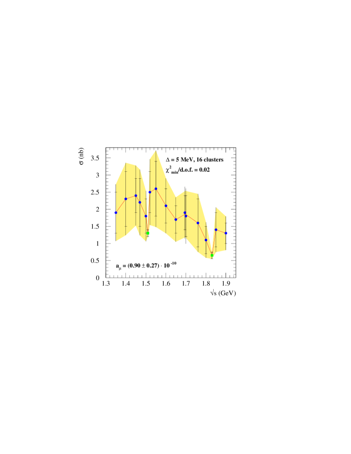
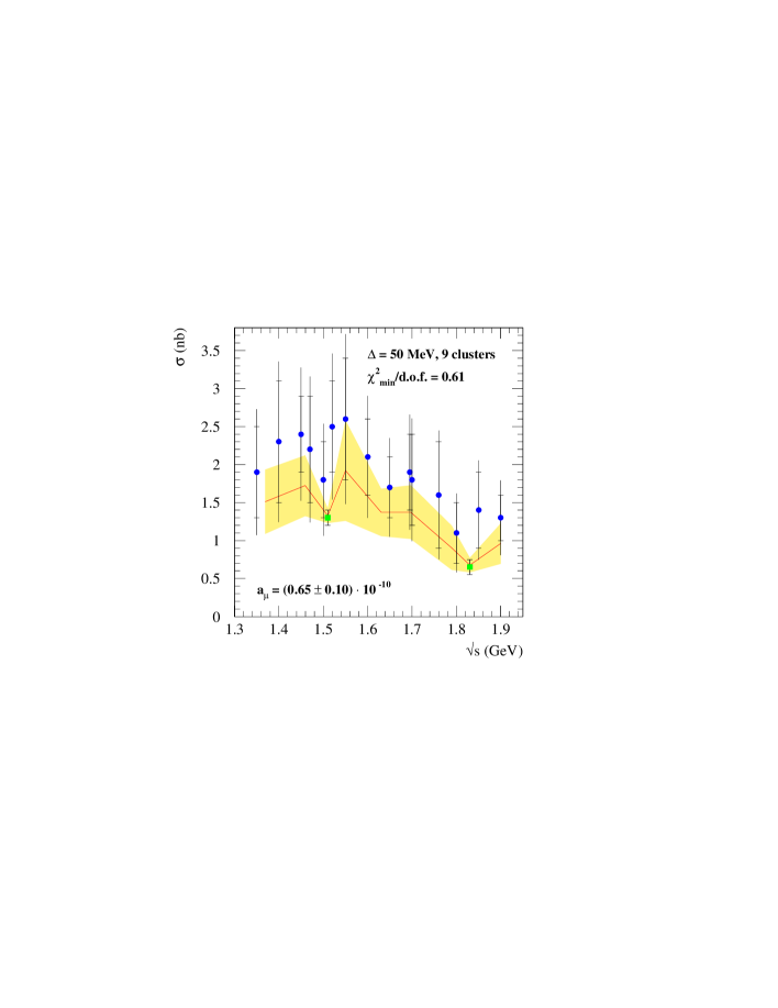
Figure 2: Two toy data sets chosen to illustrate the problems of combining precise with less precise data. The upper plot shows the result obtained with a very small ‘cluster’ size. The lower shows the data clustered in 50 MeV bins, which allows renormalization of the data within their systematic errors. Here the (much less precise) points of set 1 are renormalized by $1/1.35$ whereas the two precise points of set two are nearly unchanged ($1/0.9995$). The length of the error bars give the statistical plus systematic errors added in quadrature for each data point. The small horizontal lines in the bars indicate the size of the statistical errors. The error band of the clustered data is defined through the diagonal elements of the covariance matrix.

In order to parameterize $R(s)$ in terms of $R_{m}$, we need a prescription to determine the location of the cluster, $\sqrt{s}=E_{m}$. We proceed as follows. When the original data points, which contribute to the cluster $m$, give

$$R(\sqrt{s}=E_{i}^{\{k,m\}})\ =\ R_{i}^{\{k,m\}}\pm\sqrt{\left({\rm d}R_{i}^{\{k,m\}}\right)^{2}+\left({\rm d}f_{k}\right)^{2}}$$ (32)

from the $k$th experiment, we calculate the cluster energy $E_{m}$ by

$$E_{m}=\left[\sum_{k}\sum_{i=1}^{N_{\{k,m\}}}\frac{1}{\left({\rm d}R_{i}^{\{k,m\}}\right)^{2}+\left({\rm d}f_{k}\right)^{2}}E_{i}^{\{k,m\}}\right]\Bigg{/}\left[\sum_{k}\sum_{i=1}^{N_{\{k,m\}}}\frac{1}{\left({\rm d}R_{i}^{\{k,m\}}\right)^{2}+\left({\rm d}f_{k}\right)^{2}}\right],$$ (33)

where the sum over $k$ is for those experiments whose data points contribute to the cluster $m$. Here we use the point-to-point errors, ${\rm d}R_{i}^{\{k,m\}}$, added in quadrature with the systematic error, ${\rm d}f_{k}$, to weight the contribution of each data point to the cluster energy $E_{m}$. Alternatively, we could use just the statistical errors to determine the cluster energies $E_{m}$. We have checked that the results are only affected very slightly by this change for our chosen values for the cluster sizes.

The minimization of the non-linear $\chi^{2}$ function with respect to the free parameters $R_{m}$ and $f_{k}$ is performed numerically in an iterative procedure and we obtain the following parameterization of $R(s)$:

$$R(s=E_{m}^{2})\ \equiv\ R_{m}\ =\ \overline{R}_{m}\pm{\rm d}R_{m},$$ (34)

where the correlation between the errors ${\rm d}R_{m}$ and ${\rm d}R_{n}$,

$$\rho_{\rm corr}(m,n)=V(m,n)/({\rm d}R_{m})({\rm d}R_{n}),$$ (35)

with $V(m,m)=({\rm d}R_{m})^{2}$, is obtained from the covariance matrix $V(m,n)$ of the fit, that is

$$\chi^{2}=\chi^{2}_{\rm min}+\sum_{m=1}^{N_{\rm clust}}\sum_{n=1}^{N_{\rm clust}}(R_{m}-\overline{R}_{m})V^{-1}(m,n)(R_{n}-\overline{R}_{n}).$$ (36)

Here the normalization uncertainties are integrated out. We keep the fitted values of the normalization factors $f_{k}$

$$f_{k}=\bar{f}_{k}.$$ (37)

The $\chi^{2}$ function takes its minimum value $\chi^{2}_{\rm min}$ when $R_{m}=\overline{R}_{m}$ and $f_{k}=\bar{f}_{k}$. The goodness of the fit can be judged from

$$\frac{\chi^{2}_{\rm min}}{{\rm d.o.f.}}\ =\ \frac{\chi^{2}_{\rm min}}{\sum_{k}(N_{k}-1)-N_{\rm cluster}},$$ (38)

where $\sum_{k}N_{k}$ stands for the total number of data points and $\sum_{k}(-1)$ stands for the overall normalization uncertainty per experiment. Once a good fit to the function $R(s)$ is obtained, we may estimate any integral and its error as follows. Consider the definite integral

$$I(a,b)\ =\ \int_{a^{2}}^{b^{2}}{\rm d}s\,R(s)K(s)\ =\ 2\int_{a}^{b}{\rm d}E\,ER(E^{2})K(E^{2})\ =\ \bar{I}\pm\Delta I.$$ (39)

When $a=E_{m}<E_{n}=b$, the integral $I$ is estimated by the trapezoidal rule to be

$$\bar{I} = 2\left(\frac{E_{m+1}-E_{m}}{2}E_{m}R_{m}K_{m}+\frac{E_{n}-E_{n-1}}{2}E_{n}R_{n}K_{n}+\sum_{k=m+1}^{n-1}\frac{E_{k+1}-E_{k-1}}{2}E_{k}R_{k}K_{k}\right),~{}~{}~{}$$ (40)

where $K_{k}=K(E_{k}^{2})$, and its error $\Delta I$ is determined, via the covariance matrix $V$, to be

$$(\Delta I)^{2} = \sum_{k=m}^{n}~{}\sum_{l=m}^{n}\frac{\partial\bar{I}}{\partial R_{k}}V(k,l)\frac{\partial\bar{I}}{\partial R_{l}}$$ (41)

$$= \sum_{k,l=m}^{n}\left((E_{k+1}-E_{k-1})E_{k}\;K_{k}\;\right)V(k,l)\left((E_{l+1}-E_{l-1})E_{l}K_{l}\right),$$ (42)

where $E_{m-1}=E_{m}$ and $E_{n+1}=E_{n}$ at the edges, according to (40). When the integration boundaries do not match a cluster energy, we use the trapezoidal rule to interpolate between the adjacent clusters.

We have checked that for all hadronic channels we find a stable value and error for $a_{\mu}^{\rm had,LO}$, together with a good $\chi^{2}$ fit if we vary the minimal cluster size around our chosen default values (which are typically about 0.2 MeV for a narrow resonance and about 10 MeV or larger for the continuum).

Figure 3: Dependence of the fit on the cluster size parameter $\delta$ in the case of the $\pi^{+}\pi^{-}$ channel: the band in the upper plot shows the contribution to $a_{\mu}$ and its errors for different choices of the cluster size. The three lines show $\bar{a}_{\mu}$ (solid), $\bar{a}_{\mu}+\Delta a_{\mu}$ and $\bar{a}_{\mu}-\Delta a_{\mu}$ (dotted), respectively. The lower plot displays the $\chi^{2}_{\rm min}/{\rm d.o.f.}$ (continuous line) together with the error size $\Delta a_{\mu}$ in % (dashed line).

For the most important $\pi^{+}\pi^{-}$ channel we show in Fig. 3 the behaviour of the contribution to $a_{\mu}$, its error and the quality of the fit expressed through $\chi^{2}_{\rm min}/{\rm d.o.f.}$ as a function of the typical cluster size $\delta$. It is clear that very large values of $\delta$, even if they lead to a satisfactory $\chi^{2}_{\rm min}$, should be discarded as the fit would impose too much theoretical prejudice on the shape of $R(s)$. Thus, in practice, we also have to check how the curve of the clustered data, and its errors, describe the data. One would, in general, try to avoid combining together too many data points in a single cluster.

channel	data range	$\delta$ (MeV)	$\chi^{2}_{\rm min}/{\rm d.o.f.}$	range used	$a_{\mu}$	$\Delta a_{\mu}$	w/o fit
$\pi^{+}\pi^{-}$	$0.32-3$	$3.5$	$1.07$	$0.32-1.425$	$502.76$	$5.01$	$500.10$
$\pi^{+}\pi^{-}\pi^{0}$	$0.483-2.4$	$20,0.6,0.6$	$2.11$	$0.66-1.425$	$46.05$	$0.63$	$46.54$
		$20,0.2,0.2$	$1.44$	$0.66-1.425$	$46.42$	$0.76$	$47.38$
$\pi^{+}\pi^{-}\pi^{+}\pi^{-}$	$0.765-2.245$	$11$	$2.00$	$0.765-1.432$	$6.18$	$0.23$	$5.70$
$\pi^{+}\pi^{-}\pi^{0}\pi^{0}$	$0.915-2.4$	$10$	$1.28$	$0.915-1.438$	$9.89$	$0.57$	$9.44$
$K^{+}K^{-}$	$1.009-2.1$	$5,0.6$	$1.00$	$1.009-1.421$	$21.58$	$0.76$	$21.31$
$K^{0}_{S}K^{0}_{L}$	$1.004-2.14$	$10,0.1$	$0.86$	$1.004-1.442$	$13.16$	$0.16$	$13.11$
inclusive	$1.432-3.035$	$20$	$0.28$	$1.432-2.05$	$32.95$	$2.58$	$31.99$
	$2-11.09$	$20$	$0.74$	$2-11.09$	$42.02$	$1.14$	$41.51$

Table 4: Details of the clustering and fit for the dominant channels as described in the text. The values of $a_{\mu}$ and its error have been multiplied by $10^{10}$ and energy ranges are given in GeV. For the $\pi^{+}\pi^{-}\pi^{0}$ channel the bands of clustered data for $\omega$ and $\phi$ displayed in Fig. 9 were obtained using a clustering size of 0.6 MeV, which leads to a slightly worse $\chi^{2}_{\rm min}$, but a better eyeball fit, than for the 0.2 MeV clustering. For the numerics we have used the 0.2 MeV clustering size. The differences are small.

In Table 4 we give the details of the clustering and non-linear fit for the most relevant channels. The fits take into account data as cited in Table 1 with energy ranges as indicated in the second column of Table 4. We use clustering sizes $\delta$ as displayed in the third column. In the $\pi^{+}\pi^{-}\pi^{0}$, $K^{+}K^{-}$ and $K_{S}^{0}K_{L}^{0}$ channels the binning has to be very fine in the $\omega$ and $\phi$ resonance regimes; the respective values of the clustering sizes in the continuum, ($\omega$ and) $\phi$ regions are given in the Table. The $\chi^{2}_{\rm min}/{\rm d.o.f.}$ displayed in the fourth column is always good, apart from the three channels $\pi^{+}\pi^{-}\pi^{+}\pi^{-},\ \pi^{+}\pi^{-}\pi^{0}$ and $\pi^{+}\pi^{-}2\pi^{0}$, in which we inflate the error as mentioned above. In most cases the fit quality and result is amazingly stable with respect to the choice of the cluster size, indicating that no information is lost through the clustering. Table 4 also gives information about the contribution of the leading channels to $a_{\mu}$ within the given ranges. For comparison, the last column shows the contributions to $a_{\mu}$ obtained by combining data without allowing for renormalization of individual data sets through the fit parameters $f_{k}$. In this case, we use the same binning as in the full clustering, but calculate the mean values $R_{m}$ just as the weighted average of the $R$ data within a cluster:

$$R_{m}\equiv\tilde{R}_{m}=\left[\sum_{k}\sum_{i=1}^{N_{\{k,m\}}}\frac{1}{\left({\rm d}R_{i}^{\{k,m\}}\right)^{2}+\left({\rm d}f_{k}\right)^{2}}R_{i}^{\{k,m\}}\right]\Bigg{/}\left[\sum_{k}\sum_{i=1}^{N_{\{k,m\}}}\frac{1}{\left({\rm d}R_{i}^{\{k,m\}}\right)^{2}+\left({\rm d}f_{k}\right)^{2}}\right]\,.$$ (43)

(These $\tilde{R}_{m}$ values are actually used as starting values for our iterative fit procedure.) The point-to-point trapezoidal integration (40) with these $\tilde{R}_{m}$ values from (43) without the fit neglects correlations between different energies. As is clear from the comparison of columns six and eight of Table 4, such a procedure leads to wrong results, especially in the most important $\pi^{+}\pi^{-}$ channel.

As explained above, the dispersion integrals (4) and (5) are evaluated by integrating (using the trapezoidal rule (40) for the mean value and (42) for the error and thus including correlations) over the clustered data directly for all hadronic channels, including the $\omega$ and $\phi$ resonances. Thus we avoid possible problems due to missing or double-counting of non-resonant backgrounds. Moreover interference effects are taken into account automatically. As an example we display in Fig. 7 the most important $\pi^{+}\pi^{-}$ channel, together with an enlargement of the region of $\rho$–$\omega$ interference. As in Fig. 2, the error band is given by the diagonal elements of the covariance matrix of our fit, indicating the uncertainty of the mean values. Data points are displayed (here and in the following) after application of radiative corrections. The error bars show the statistical and systematic errors added in quadrature and the horizontal markers inside the error bars indicate the size of the statistical error alone.

In the region between $1.43$ and $\sim 2$ GeV we have the choice between summing up the exclusive channels or relying on the inclusive measurements from the $\gamma\gamma 2$, MEA, M3N and ADONE experiments [84]–[87]. Two-body final states were not included in these analyses. Therefore we correct the $R$ data from $\gamma\gamma 2$, MEA and ADONE for missing contributions from $\pi^{+}\pi^{-}$, $K^{+}K^{-}$ and $K^{0}_{S}K^{0}_{L}$, estimating them from our exclusive data compilation. The corrections are small compared to the large statistical and systematic errors and energy dependent, ranging from up to 7% at 1.4 GeV down to about 3% at 2 GeV. In addition, we add some purely neutral modes to the inclusive data, see below. Surprisingly, even after having applied these corrections, the sum of exclusive channels overshoots the inclusive data. The discrepancy is shown in Fig. 4, where we display the results of our clustering algorithm for the inclusive and the sum of exclusive data including error bars defined by the diagonal elements of the covariance matrices (errors added in quadrature for the exclusive channels). We study the problem of this exclusive/inclusive discrepancy in detail in Section 4.

Figure 4: The behaviour of $R$ obtained from inclusive data and from the sum of exclusive channels, after clustering and fitting the various data sets. Note the suppressed zero of the vertical scale.

3 Evaluation of the dispersion relations for $a_{\mu}^{\rm had,LO}$ and $\Delta\alpha_{\rm had}$

Here we use dispersion relations (4) and (5) to determine $a_{\mu}^{\rm had,LO}$ and $\Delta\alpha_{\rm had}(M_{Z}^{2})$ respectively, which in turn we will use to predict $g-2$ of the muon (in Section 7) and the QED coupling $\alpha(M_{Z}^{2})$ (in Section 8). The dispersion relation (4) has the form

$$a_{\mu}^{\rm had,LO}=\frac{1}{4\pi^{3}}\int_{s_{\rm th}}^{\infty}{\rm d}s\ \sigma_{\rm had}^{0}(s)\left(\frac{m_{\mu}^{2}}{3s}\ K(s)\right),$$ (44)

where $\sigma_{\rm had}^{0}(s)$ is the total cross section for $e^{+}e^{-}\to{\rm hadrons}\,(+\gamma)$ at centre-of-mass energy $\sqrt{s}$, as defined in (2). For $s>4m_{\mu}^{2}$ the kernel function $K(s)$ is given by [112]

$$K(s>4m_{\mu}^{2})=\frac{3s}{m_{\mu}^{2}}\left\{\frac{x^{2}}{2}(2-x^{2})+\frac{(1+x^{2})(1+x)^{2}}{x^{2}}\left(\ln(1+x)-x+\frac{x^{2}}{2}\right)+\frac{1+x}{1-x}x^{2}\ln x\right\},$$ (45)

with $x\equiv(1-\beta_{\mu})/(1+\beta_{\mu})$ where $\beta_{\mu}\equiv\sqrt{1-4m_{\mu}^{2}/s}$; while for $s<4m_{\mu}^{2}$ the form of the kernel can be found in [113], and is used to evaluate the small $\pi^{0}\gamma$ contribution to $a_{\mu}^{\rm had,LO}$. Dispersion relation (5), evaluated at $s=M_{Z}^{2}$, may be written in the form

$$\Delta\alpha_{\rm had}(M_{Z}^{2})=-\frac{M_{Z}^{2}}{4\pi^{2}\alpha}{\rm P}\int_{s_{\rm th}}^{\infty}{\rm d}s\,\frac{\sigma_{\rm had}^{0}(s)}{s-M_{Z}^{2}}\,.$$ (46)

To evaluate (44) and (46) we need to input the function $\sigma_{\rm had}^{0}(s)$ and its error. Up to $\sqrt{s}\sim 2~{}{\rm GeV}$ we can calculate $\sigma_{\rm had}^{0}$ from the sum of the cross sections for all the exclusive channels $e^{+}e^{-}\to\pi^{+}\pi^{-},\pi^{+}\pi^{-}\pi^{0}$, etc. On the other hand for $\sqrt{s}\;\raisebox{-3.01385pt}{$\stackrel{{\scriptstyle\textstyle>}}{{\sim}}$}\;1.4~{}{\rm GeV}$ the value of $\sigma_{\rm had}^{0}$ can be obtained from inclusive measurements of $e^{+}e^{-}\to{\rm hadrons}$. Thus, as mentioned above, there is an ‘exclusive, inclusive overlap’ in the interval $1.4\;\raisebox{-3.01385pt}{$\stackrel{{\scriptstyle\textstyle<}}{{\sim}}$}\;\sqrt{s}\;\raisebox{-3.01385pt}{$\stackrel{{\scriptstyle\textstyle<}}{{\sim}}$}\;2~{}{\rm GeV}$, which allows a comparison of the two methods of determining $\sigma_{\rm had}^{0}$ from the data. As we have seen, the two determinations do not agree, see Fig. 4. It is worth noting that the data in this interval come from older experiments. The new, higher precision, Novosibirsk data on the exclusive channels terminate at $\sqrt{s}\sim 1.4~{}{\rm GeV}$, and the recent inclusive BES data [88, 89] start only at $\sqrt{s}\sim 2~{}{\rm GeV}$. Thus in Table 5 we show the contributions of the individual channels to $a_{\mu}^{\rm had,LO}$ and $\Delta\alpha_{\rm had}(M_{Z}^{2})$ using first inclusive data in the interval $1.43<\sqrt{s}<2~{}{\rm GeV}$, and then replacing them by the sum of the exclusive channels.

channel	inclusive (1.43,2 GeV)		exclusive (1.43,2 GeV)
	$a_{\mu}^{\rm had,LO}$	$\Delta\alpha_{\rm had}(M_{Z}^{2})$	$a_{\mu}^{\rm had,LO}$	$\Delta\alpha_{\rm had}(M_{Z}^{2})$
$\pi^{0}\gamma$ (ChPT)	$0.13\pm 0.01$	$0.00\pm 0.00$	$0.13\pm 0.01$	$0.00\pm 0.00$
$\pi^{0}\gamma$ (data)	$4.50\pm 0.15$	$0.36\pm 0.01$	$4.50\pm 0.15$	$0.36\pm 0.01$
$\pi^{+}\pi^{-}$ (ChPT)	$2.36\pm 0.05$	$0.04\pm 0.00$	$2.36\pm 0.05$	$0.04\pm 0.00$
$\pi^{+}\pi^{-}$ (data)	$502.78\pm 5.02$	$34.39\pm 0.29$	$503.38\pm 5.02$	$34.59\pm 0.29$
$\pi^{+}\pi^{-}\pi^{0}$ (ChPT)	$0.01\pm 0.00$	$0.00\pm 0.00$	$0.01\pm 0.00$	$0.00\pm 0.00$
$\pi^{+}\pi^{-}\pi^{0}$ (data)	$46.43\pm 0.90$	$4.33\pm 0.08$	$47.04\pm 0.90$	$4.52\pm 0.08$
$\eta\gamma$ (ChPT)	$0.00\pm 0.00$	$0.00\pm 0.00$	$0.00\pm 0.00$	$0.00\pm 0.00$
$\eta\gamma$ (data)	$0.73\pm 0.03$	$0.09\pm 0.00$	$0.73\pm 0.03$	$0.09\pm 0.00$
$K^{+}K^{-}$	$21.62\pm 0.76$	$3.01\pm 0.11$	$22.35\pm 0.77$	$3.23\pm 0.11$
$K_{S}^{0}K_{L}^{0}$	$13.16\pm 0.31$	$1.76\pm 0.04$	$13.30\pm 0.32$	$1.80\pm 0.04$
$2\pi^{+}2\pi^{-}$	$6.16\pm 0.32$	$1.27\pm 0.07$	$14.77\pm 0.76$	$4.04\pm 0.21$
$\pi^{+}\pi^{-}2\pi^{0}$	$9.71\pm 0.63$	$1.86\pm 0.12$	$20.55\pm 1.22$	$5.51\pm 0.35$
$2\pi^{+}2\pi^{-}\pi^{0}$	$0.26\pm 0.04$	$0.06\pm 0.01$	$2.85\pm 0.25$	$0.99\pm 0.09$
$\pi^{+}\pi^{-}3\pi^{0}$	$0.09\pm 0.09$	$0.02\pm 0.02$	$1.19\pm 0.33$	$0.41\pm 0.10$
$3\pi^{+}3\pi^{-}$	$0.00\pm 0.00$	$0.00\pm 0.00$	$0.22\pm 0.02$	$0.09\pm 0.01$
$2\pi^{+}2\pi^{-}2\pi^{0}$	$0.12\pm 0.03$	$0.03\pm 0.01$	$3.32\pm 0.29$	$1.22\pm 0.11$
$\pi^{+}\pi^{-}4\pi^{0}$ (isospin)	$0.00\pm 0.00$	$0.00\pm 0.00$	$0.12\pm 0.12$	$0.05\pm 0.05$
$K^{+}K^{-}\pi^{0}$	$0.00\pm 0.00$	$0.00\pm 0.00$	$0.29\pm 0.07$	$0.10\pm 0.03$
$K_{S}^{0}K_{L}^{0}\pi^{0}$ (isospin)	$0.00\pm 0.00$	$0.00\pm 0.00$	$0.29\pm 0.07$	$0.10\pm 0.03$
$K_{S}^{0}\pi^{\mp}K^{\pm}$	$0.05\pm 0.02$	$0.01\pm 0.00$	$1.00\pm 0.11$	$0.33\pm 0.04$
$K_{L}^{0}\pi^{\mp}K^{\pm}$ (isospin)	$0.05\pm 0.02$	$0.01\pm 0.00$	$1.00\pm 0.11$	$0.33\pm 0.04$
$K\bar{K}\pi\pi$ (isospin)	$0.00\pm 0.00$	$0.00\pm 0.00$	$3.63\pm 1.34$	$1.33\pm 0.48$
$\omega(\to\pi^{0}\gamma)\pi^{0}$	$0.64\pm 0.02$	$0.12\pm 0.00$	$0.83\pm 0.03$	$0.17\pm 0.01$
$\omega(\to\pi^{0}\gamma)\pi^{+}\pi^{-}$	$0.01\pm 0.00$	$0.00\pm 0.00$	$0.07\pm 0.01$	$0.02\pm 0.00$
$\eta(\to\pi^{0}\gamma)\pi^{+}\pi^{-}$	$0.07\pm 0.01$	$0.02\pm 0.00$	$0.49\pm 0.07$	$0.15\pm 0.02$
$\phi(\to{\rm unaccounted})$	$0.06\pm 0.06$	$0.01\pm 0.01$	$0.06\pm 0.06$	$0.01\pm 0.01$
$p\bar{p}$	$0.00\pm 0.00$	$0.00\pm 0.00$	$0.04\pm 0.01$	$0.02\pm 0.00$
$n\bar{n}$	$0.00\pm 0.00$	$0.00\pm 0.00$	$0.07\pm 0.02$	$0.03\pm 0.01$
$J/\psi,\psi^{\prime}$	$7.30\pm 0.43$	$8.90\pm 0.51$	$7.30\pm 0.43$	$8.90\pm 0.51$
$\Upsilon(1S-6S)$	$0.10\pm 0.00$	$1.16\pm 0.04$	$0.10\pm 0.00$	$1.16\pm 0.04$
inclusive $R$	$73.96\pm 2.68$	$92.75\pm 1.74$	$42.05\pm 1.14$	$81.97\pm 1.53$
pQCD	$2.11\pm 0.00$	$125.32\pm 0.15$	$2.11\pm 0.00$	$125.32\pm 0.15$
sum	$692.38\pm 5.88$	$275.52\pm 1.85$	$696.15\pm 5.68$	$276.90\pm 1.77$

Table 5: Contributions to the dispersion relations (4) and (5) from the individual channels.

Below we describe, in turn, how the contributions of each channel have been evaluated. First we note that narrow $\omega$ and $\phi$ contributions to the appropriate channels are obtained by integrating over the (clustered) data using the trapezoidal rule. We investigated the use of parametric Breit–Wigner forms by fitting to the data over various mass ranges. We found no significant change in the contributions if the resonant parameterization was used in the region of the $\omega$ and $\phi$ peaks, but that the contributions of the resonance tails depend a little on the parametric form used. The problem did not originate from a bias due to the use of the linear trapezoidal rule in a region where the resonant form was concave, but rather was due to the fact that different resonant forms fitted better to different points in the tails. For this reason we believe that it is more reliable to rely entirely on the data, which are now quite precise in the resonance regions.

3.1 $\pi^{0}\gamma$ channel

The contribution of the $e^{+}e^{-}\to\pi^{0}\gamma$ channel defines the lower limit, $\sqrt{s}_{\rm th}=m_{\pi}$, of the dispersion integrals. There exist two data sets [31, 32] for this channel, which cover the interval $0.60<\sqrt{s}<1.03~{}{\rm GeV}$ (see Fig. 5). After clustering, a trapezoidal rule integration over this $\pi^{0}\gamma$ energy interval gives a contribution

$$a_{\mu}(\pi^{0}\gamma,\,0.6<\sqrt{s}<1.03~{}{\rm GeV})=(4.50\pm 0.15)\times 10^{-10}$$ (47)

and

$$\Delta\alpha_{\rm had}(\pi^{0}\gamma,\,0.6<\sqrt{s}<1.03~{}{\rm GeV})=(0.36\pm 0.01)\times 10^{-4}.$$ (48)

In Fig. 5 we show an overall picture of the $e^{+}e^{-}\to\pi^{0}\gamma$ data and a blow up around the $\rho$-$\omega$ region.

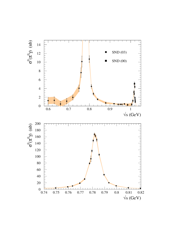
Figure 5: Data for $\sigma^{0}(e^{+}e^{-}\to\pi^{0}\gamma)$. The shaded band shows the behaviour of the cross section after clustering and fitting the data. The second plot is an enlargement in the region of the $\omega$ resonance.

The use of the trapezoidal rule for the interval $m_{\pi}<\sqrt{s}<0.6~{}{\rm GeV}$ would overestimate the contribution, since the cross section is not linear in $\sqrt{s}$. In this region we use chiral perturbation theory (ChPT), based on the Wess–Zumino–Witten (WZW) local interaction for the $\pi^{0}\gamma\gamma$ vertex,

$${\cal L}_{WZW}=-\frac{\alpha}{8\pi f_{\pi}}\pi^{0}\epsilon^{\mu\nu\lambda\sigma}F_{\mu\nu}F_{\lambda\sigma},$$ (49)

with $f_{\pi}\simeq 93$ MeV, which yields

$$\sigma(e^{+}e^{-}\to\pi^{0}\gamma)=\sigma_{\rm pt}\equiv\frac{8\alpha\pi\Gamma(\pi^{0}\to 2\gamma)}{3m_{\pi}^{3}}\left(1-\frac{m_{\pi}^{2}}{s}\right)^{3}.$$ (50)

Since the electromagnetic current couples to $\pi^{0}\gamma$ via $\omega$ meson exchange, the low-energy cross section can be improved by assuming the $\omega$-meson dominance [113], which gives

$$\sigma_{\rm VMD}(e^{+}e^{-}\to\pi^{0}\gamma)=\sigma_{\rm pt}(e^{+}e^{-}\to\pi^{0}\gamma)\left(\frac{m_{\omega}^{2}}{m_{\omega}^{2}-s}\right)^{2}.$$ (51)

We find

$$a_{\mu}(\pi^{0}\gamma,\sqrt{s}<0.6~{}{\rm GeV})=(0.13\pm 0.01)\times 10^{-10},$$ (52)

while the contribution to $\Delta\alpha_{\rm had}$ is less than $10^{-6}$. The agreement of the prediction of (51) for the $\pi^{0}\gamma$ cross section with the SND data just above 0.6 GeV is shown in Fig. 6.

Figure 6: Predictions for $\sigma^{0}(e^{+}e^{-}\to\pi^{0}\gamma)$ from ChPT compared with low energy experimental data from the SND collaboration [31]. In the figure we have multiplied $m^{2}_{\mu}/(3s)K(s)$ by the cross section so that the area below the data is proportional to the contribution to $a_{\mu}$. The continuous curve, which is obtained assuming Vector Meson ($\omega$) Dominance (VMD), is used for $s<0.36~{}{\rm GeV}^{2}$.

3.2 $\pi^{+}\pi^{-}$ channel

We use 16 data sets for $e^{+}e^{-}\to\pi^{+}\pi^{-}$ [10], [16]–[30] which cover the energy range $0.32<\sqrt{s}<3.0~{}{\rm GeV}$. Some older data with very large errors are omitted. In Fig. 7, we show the region around $\rho$, which gives the most important contribution to $g-2$ of the muon.

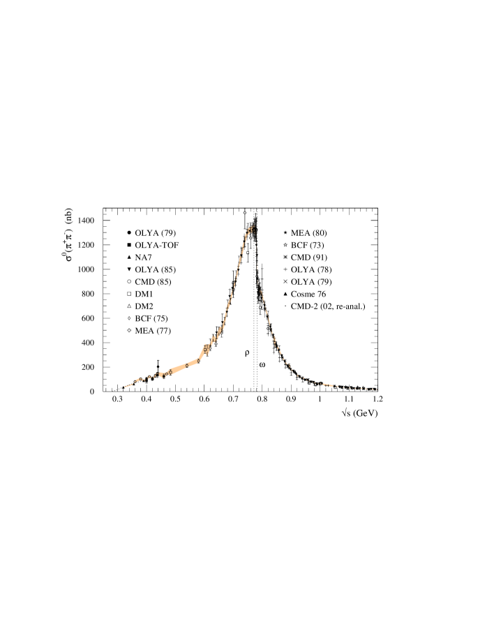
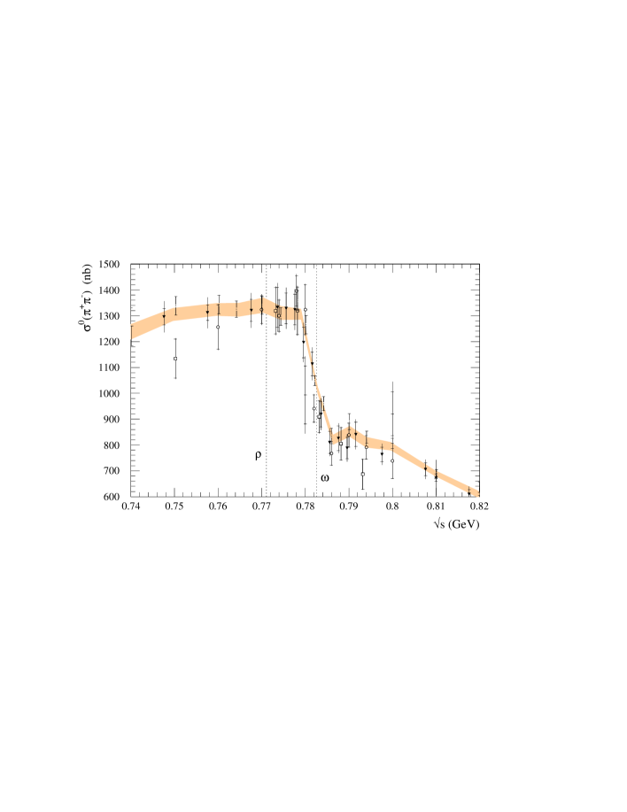
Figure 7: $e^{+}e^{-}\to\pi^{+}\pi^{-}$ data up to 1.2 GeV, after radiative corrections, where the shaded band shows the result, $\sigma^{0}(\pi^{+}\pi^{-})$ (obtained from $R_{m}$ of (31)), of our fit after clustering. The width of the band indicates the error on the $\sigma^{0}(\pi^{+}\pi^{-})$ values, obtained from the diagonal elements of the full covariance matrix. The second plot is an enlargement of the $\rho$-$\omega$ interference region.

The $\pi^{+}\pi^{-}$ contributions to $a_{\mu}^{\rm had,LO}$ and $\Delta\alpha_{\rm had}(M_{Z}^{2})$, obtained by integrating clustered data over various energy intervals, are shown in Table 6.

$\sqrt{s}~{}({\rm GeV})$		comment	$a_{\mu}^{\rm had,LO}\times 10^{10}$		$\Delta\alpha_{\rm had}(M_{Z}^{2})\times 10^{4}$
0.32–	1.43		502.78$~{}\pm$	5.02	34.39$~{}\pm$	0.29
(0.32–	1.43	‘old’ CMD-2	492.66$~{}\pm$	4.93	33.65$~{}\pm$	0.28)
0.32–	2		503.38$~{}\pm$	5.02	34.59$~{}\pm$	0.29
0–	0.32	ChPT	2.36$~{}\pm$	0.05	0.04$~{}\pm$	0.00

Table 6: $\pi^{+}\pi^{-}$ contributions to $a_{\mu}^{\rm had,LO}$ and $\Delta\alpha_{\rm had}(M_{Z}^{2})$ from various energy intervals. The entries in brackets give the contributions obtained using the CMD-2 data before re-analysis.

As seen from the Table, if we integrate over the data up to 1.43 GeV, we obtain

$$a_{\mu}(\pi^{+}\pi^{-},0.32<\sqrt{s}<1.43~{}{\rm GeV}) = (502.78\pm 5.02)\times 10^{-10},$$ (53)

$$\Delta\alpha_{\rm had}(\pi^{+}\pi^{-},0.32<\sqrt{s}<1.43~{}{\rm GeV}) = (34.39\pm 0.29)\times 10^{-4}.$$ (54)

If we integrate up to 2 GeV, instead of 1.43 GeV, we obtain

$$a_{\mu}(\pi^{+}\pi^{-},0.32<\sqrt{s}<2~{}{\rm GeV}) = (503.38\pm 5.02)\times 10^{-10},$$ (55)

$$\Delta\alpha_{\rm had}(\pi^{+}\pi^{-},0.32<\sqrt{s}<2~{}{\rm GeV}) = (34.59\pm 0.29)\times 10^{-4}.$$ (56)

The contribution of the $\pi^{+}\pi^{-}$ channel is dominated by the $\rho$-meson, and hence the differences between Eqs. (53) and (55) is small. If we use the CMD-2 data before the recent re-analysis [10], we have

$$a_{\mu}(\pi^{+}\pi^{-},0.32<\sqrt{s}<1.43~{}{\rm GeV},{\rm~{}old~{}CMD\mbox{-}2~{}data}) = (492.66\pm 4.93)\times 10^{-10},$$ (57)

$$\Delta\alpha_{\rm had}(\pi^{+}\pi^{-},0.32<\sqrt{s}<1.43~{}{\rm GeV},{\rm~{}old~{}CMD\mbox{-}2~{}data}) = (33.65\pm 0.28)\times 10^{-4}.$$ (58)

The comparison of (53) and (57) shows the effect of the re-analysis of the recent CMD-2 data, which is an upward shift of the central value by roughly 2% in this interval.

It is interesting to quantify the prominent role of these most precise CMD-2 $e^{+}e^{-}\to\pi^{+}\pi^{-}$ data, which have a systematic error of only 0.6%. If we were to omit these CMD-2 data in the central $\rho$ regime altogether, the contribution of this channel to $a_{\mu}$ would decrease by roughly $12.1\times 10^{-10}$, i.e., by $\sim 2.4\%$, whereas the error would increase by about $3.4\times 10^{-10}$, i.e., by $\sim 68\%$ in the interval $0.32<\sqrt{s}<1.43$ GeV.

In the threshold region, below 0.32 GeV, we use chiral perturbation theory, due to the lack of $\pi^{+}\pi^{-}$ experimental data. The pion form factor $F_{\pi}(s)$ is written as

$$F_{\pi}(s)=1+\frac{1}{6}\langle r^{2}\rangle_{\pi}s+c_{\pi}s^{2}+{\cal O}(s^{3}),$$ (59)

with coefficients determined to be [114]

$$\langle r^{2}\rangle_{\pi}=0.431\pm 0.026~{}({\rm fm}^{2}),~{}~{}~{}~{}c_{\pi}=3.2\pm 1.0~{}({\rm GeV}^{-4}),$$ (60)

by fitting to space-like pion scattering data [115]. Fig. 8 compares the prediction with the (time-like) experimental data which exist for $\sqrt{s}\geq 0.32~{}{\rm GeV}$.

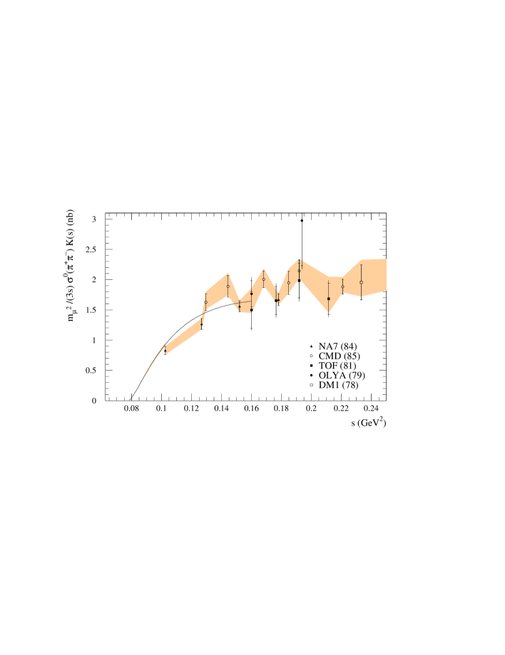
Figure 8: The $e^{+}e^{-}\to\pi^{+}\pi^{-}$ data near the threshold. In the figure we have multiplied $m^{2}_{\mu}/(3s)K(s)$ by the cross section so that the area below the data is proportional to the contribution to $a_{\mu}$. The theoretical curve obtained from chiral perturbation theory is also shown, and is used up to $\sqrt{s}=0.32~{}{\rm GeV}$ ($s=0.10~{}{\rm GeV}^{2}$).

The contributions from the threshold region are

$$a_{\mu}(\pi^{+}\pi^{-},\sqrt{s}<0.32~{}{\rm GeV}) = (2.36\pm 0.05)\times 10^{-10},$$ (61)

$$\Delta\alpha_{\rm had}(\pi^{+}\pi^{-},\sqrt{s}<0.32~{}{\rm GeV}) = (0.04\pm 0.00)\times 10^{-4},$$ (62)

and are also listed in the last row of Table 6. Though these contributions are small, for $a_{\mu}$ it is non-negligible.

In the calculation of the contribution from the threshold region, we have included the effect from final state (FS) radiative corrections. In Ref. [102] both the ${\cal O}(\alpha)$ correction and the exponentiated formula for the FS corrections are given. If we do not apply the FS correction, we would obtain

$$a_{\mu}(\pi^{+}\pi^{-},\sqrt{s}<0.32{\rm~{}GeV})=(2.30\pm 0.05)\times 10^{-10}.$$ (63)

However, if we include the FS corrections, we have

$$a_{\mu}(\pi^{+}\pi^{-},\sqrt{s}<0.32{\rm~{}GeV},{\cal O}(\alpha){\rm~{}FS~{}corr.}) = (2.36\pm 0.05)\times 10^{-10}.$$ (64)

We obtain the same contribution if we use the exponentiated formula, which we have used in all the tables in the paper. The effect of final state radiation is to increase the contribution by about 3 %, whether the ${\cal O}(\alpha)$ or the exponentiated form is used. Similarly, the contribution from this region to $\Delta\alpha_{\rm had}(M_{Z}^{2})$ is given by

$$\Delta\alpha_{\rm had}(\pi^{+}\pi^{-},\sqrt{s}<0.32{\rm~{}GeV},{\rm exponentiated~{}FS~{}corr.}) = (0.04\pm 0.00)\times 10^{-4},$$ (65)

so here the contribution from the threshold region is totally negligible.

3.3 $\pi^{+}\pi^{-}\pi^{0}$ channel

We use ten experimental data sets for the $\pi^{+}\pi^{-}\pi^{0}$ channel [10, 13, 22, 34], [37]–[42], which extend up to 2.4 GeV, although the earlier experiments have large errors, see Fig. 9. Since the data for this channel are not very good, we inflate the error by a factor of $\sqrt{\chi^{2}_{\rm min}/{\rm d.o.f.}}$, which is 1.20 for this channel. (We inflate the error by a factor of $\sqrt{\chi^{2}_{\rm min}/{\rm d.o.f.}}$ whenever $\chi^{2}_{\rm min}/{\rm d.o.f.}>1.2$, as discussed in Section 2.4, see Table 4.)

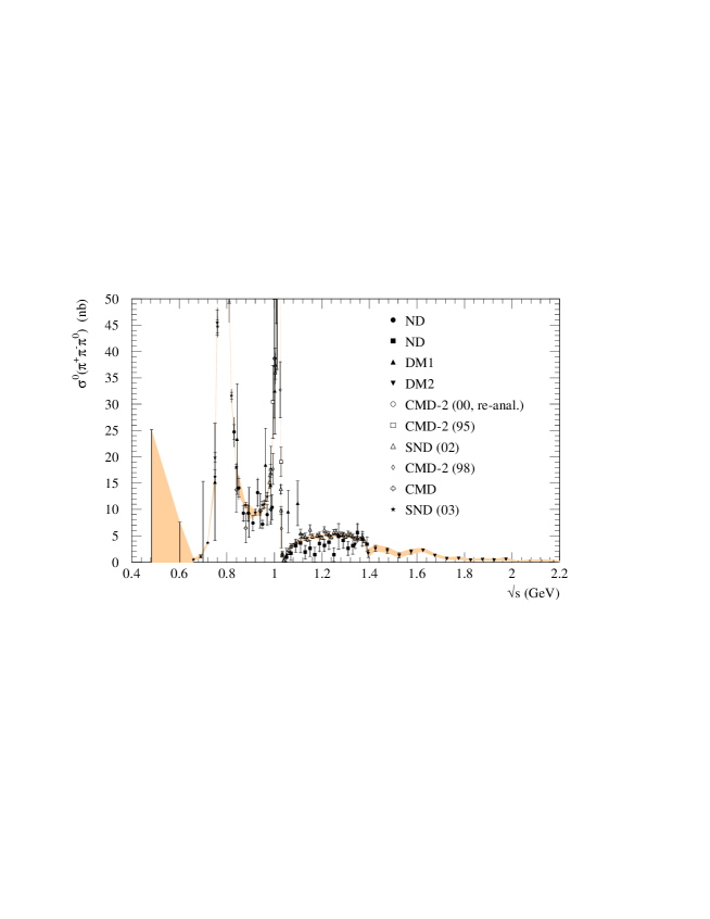
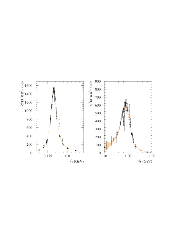
Figure 9: The data for $\sigma^{0}(e^{+}e^{-}\to\pi^{+}\pi^{-}\pi^{0})$ together with an expanded version in the $\omega$ and $\phi$ resonance regions. The shaded band shows the result of our fit after clustering. In the analysis we do not use the first two data points, below 0.66 GeV, but use chiral perturbation theory as shown in Fig. 10.

We discard the data points below 0.66 GeV, in favour of the predictions of chiral perturbation theory [116, 117], see Fig. 10. The contributions to $a_{\mu}^{\rm had,LO}$ and $\Delta\alpha_{\rm had}(M_{Z}^{2})$ are

$$a_{\mu}(\pi^{+}\pi^{-}\pi^{0},0.66{\rm~{}GeV}<\sqrt{s}<1.43{\rm~{}GeV},{\rm~{}data}) = (46.43\pm 0.90)\times 10^{-10},$$ (66)

$$\Delta\alpha_{\rm had}(\pi^{+}\pi^{-}\pi^{0},0.66{\rm~{}GeV}<\sqrt{s}<1.43{\rm~{}GeV},{\rm~{}data}) = (4.33\pm 0.08)\times 10^{-4},$$ (67)

respectively.

In the threshold region, below 0.66 GeV, we use chiral perturbation theory [116, 117], due to the lack of good $\pi^{+}\pi^{-}\pi^{0}$ experimental data, see Figs. 9 and 10.

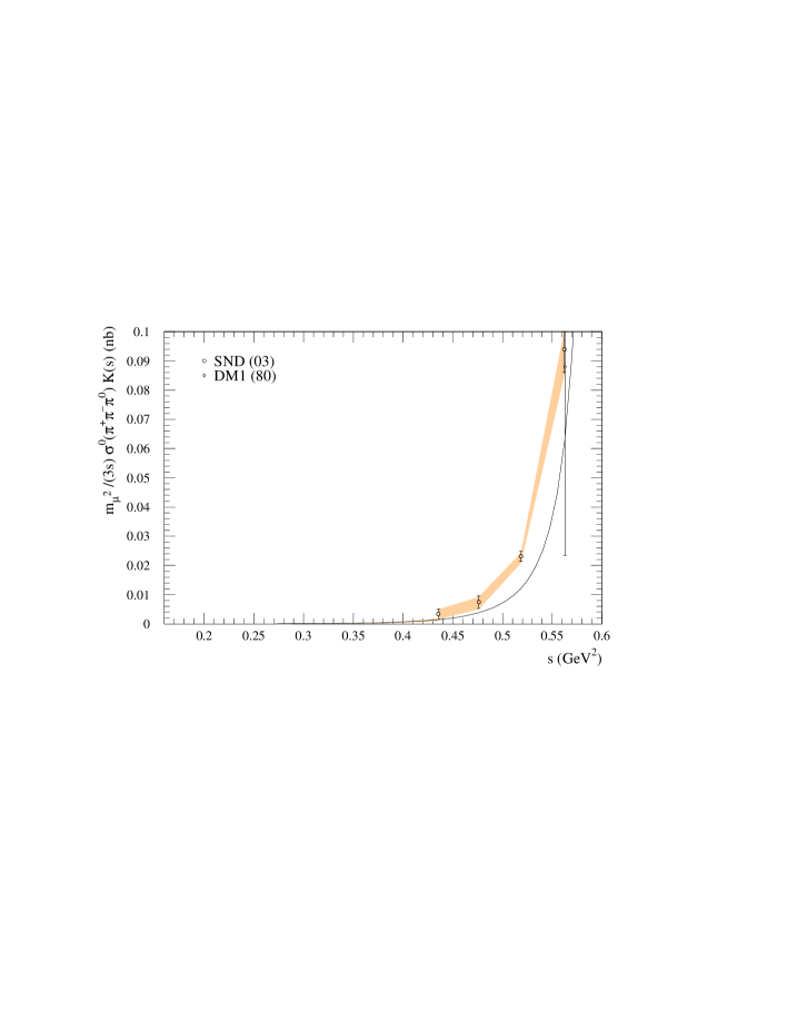
Figure 10: $e^{+}e^{-}\to\pi^{+}\pi^{-}\pi^{0}$ data [37, 41] near the threshold compared with the predictions of chiral perturbation theory. Three measurements [37] of zero cross section with very large errors are not shown. In the figure we have multiplied $m^{2}_{\mu}/(3s)K(s)$ by the cross section so that the area below the data is proportional to the contribution to $a_{\mu}$. The theoretical curve obtained from chiral perturbation theory is used up to $\sqrt{s}=0.66~{}{\rm GeV}$ ($s=0.44$ GeV²).

The contributions to $a_{\mu}^{\rm had,LO}$ and $\Delta\alpha_{\rm had}(M_{Z}^{2})$ from the threshold region are

$$a_{\mu}(\pi^{+}\pi^{-}\pi^{0},\sqrt{s}<0.66~{}{\rm GeV},~{}{\rm ChPT}) = (0.01\pm 0.00)\times 10^{-10},$$ (68)

$$\Delta\alpha_{\rm had}(\pi^{+}\pi^{-}\pi^{0},\sqrt{s}<0.66~{}{\rm GeV},~{}{\rm ChPT}) = (0.00\pm 0.00)\times 10^{-4}.$$ (69)

There is a tendency that the ChPT prediction with the $\omega$-dominance undershoots the lowest-energy data points. Because of the smallness of the threshold contribution, we do not attempt further improvement of the analysis.

3.4 $\eta\gamma$ channel

We use five data sets from SND [32, 33] and CMD-2 [34, 35, 36]. We divide the data set given in Ref. [36] into two parts at 0.95 GeV since it has different systematic errors below and above this energy.

Since the lowest data point starts only at 690 MeV, we use ChPT at the threshold region up to the lowest-energy data point. We summarize our method in Appendix A, according to which the contribution from the region to $a_{\mu}^{\rm had,LO}$ is less than $10^{-12}$, which can be safely neglected. The contribution to $\Delta\alpha_{\rm had}$ is also small, and less than $10^{-7}$. In Fig. 11 we show the threshold region of the $\eta\gamma$ production cross section and our prediction from ChPT.

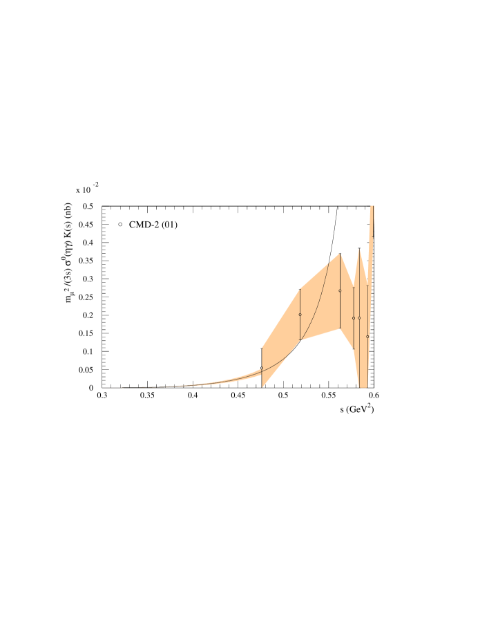
Figure 11: $e^{+}e^{-}\to\eta\gamma$ data near the threshold compared with the predictions of chiral perturbation theory.

Above the lowest-energy data point we integrate over the data. In Fig. 12 we show the overall picture of the $\eta\gamma$ production cross section and our result of the clustering. After integrating over $0.69<\sqrt{s}<1.43$ GeV we obtain

$$a_{\mu}(\eta\gamma,0.69<\sqrt{s}<1.43~{}{\rm GeV}) = (0.73\pm 0.03)\times 10^{-10},$$ (70)

$$\Delta\alpha_{\rm had}(\eta\gamma,0.69<\sqrt{s}<1.43~{}{\rm GeV}) = (0.09\pm 0.00)\times 10^{-4}.$$ (71)

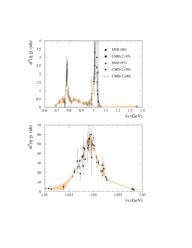
Figure 12: An overall picture of the $e^{+}e^{-}\to\eta\gamma$ data together with an enlargement in the region of the $\phi$ resonance.

3.5 $4\pi,5\pi,6\pi$ and $\eta\pi^{+}\pi^{-}$ channels

For the $4\pi$ channel, we have data for the $2\pi^{+}2\pi^{-}$ and the $\pi^{+}\pi^{-}2\pi^{0}$ final states. (The reaction $e^{+}e^{-}\to\gamma^{\ast}\to 4\pi^{0}$ is forbidden from charge conjugation symmetry.)

For the $2\pi^{+}2\pi^{-}$ channel, we use thirteen data sets [22, 50, 51], [53]–[55], [62]–[68], see Fig. 13.

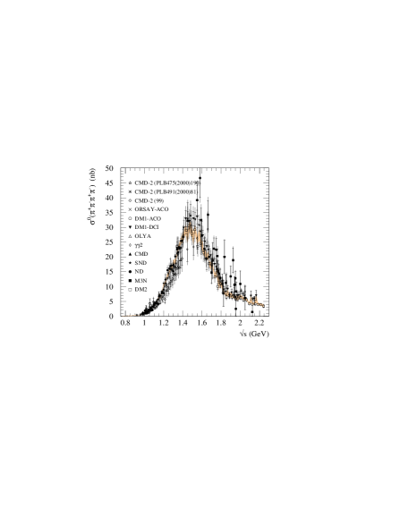
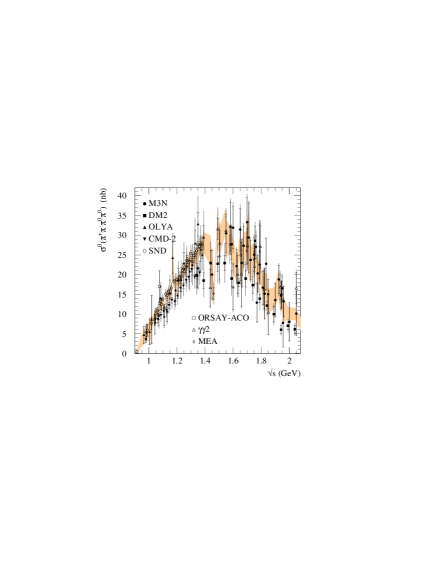
Figure 13: The data for $\sigma^{0}(e^{+}e^{-}\to 2\pi^{+}2\pi^{-})$ (left) and $\sigma^{0}(e^{+}e^{-}\to\pi^{+}\pi^{-}2\pi^{0})$ (right).

Since the data for this channel are not very consistent to each other, we inflate the error by a factor of $\sqrt{\chi^{2}_{\rm min}/{\rm d.o.f.}}=1.41$. We note, in particular, that the compatibility between the data from SND and CMD-2 is poor. This may improve after the re-analysis of the CMD-2 data for this channel is completed [111]. The contribution from this channel is

$$a_{\mu}(2\pi^{+}2\pi^{-},\sqrt{s}<1.43~{}{\rm GeV},~{}{\rm data}) = (6.16\pm 0.32)\times 10^{-10},$$ (72)

$$\Delta\alpha_{\rm had}(2\pi^{+}2\pi^{-},\sqrt{s}<1.43~{}{\rm GeV},~{}{\rm data}) = (1.27\pm 0.07)\times 10^{-4}.$$ (73)

For the $\pi^{+}\pi^{-}2\pi^{0}$ channel, we use eight data sets [50]–[57], see Fig. 13, which contribute

$$a_{\mu}(\pi^{+}\pi^{-}2\pi^{0},\sqrt{s}<1.43~{}{\rm GeV},~{}{\rm data}) = (9.71\pm 0.63)\times 10^{-10},$$ (74)

$$\Delta\alpha_{\rm had}(\pi^{+}\pi^{-}2\pi^{0},\sqrt{s}<1.43~{}{\rm GeV},~{}{\rm data}) = (1.86\pm 0.12)\times 10^{-4}.$$ (75)

For the $\pi^{+}\pi^{-}2\pi^{0}$ channel we have inflated the error by $\sqrt{\chi^{2}_{\rm min}/{\rm d.o.f.}}=1.13$ as discussed in Section 2.4.

For the $5\pi$ channel, there exist data for the $2\pi^{+}2\pi^{-}\pi^{0}$ and the $\pi^{+}\pi^{-}3\pi^{0}$ final states. (The reaction $e^{+}e^{-}\to\gamma^{\ast}\to 5\pi^{0}$ is forbidden from charge conjugation symmetry.) We use five data sets for the $2\pi^{+}2\pi^{-}\pi^{0}$ channel [22, 50, 56, 57, 62], and one data set for the $\pi^{+}\pi^{-}3\pi^{0}$ channel [50]. We integrate over the clustered data, which gives

$$a_{\mu}(2\pi^{+}2\pi^{-}\pi^{0},\sqrt{s}<1.43~{}{\rm GeV},~{}{\rm data}) = (0.26\pm 0.04)\times 10^{-10},$$ (76)

$$\Delta\alpha_{\rm had}(2\pi^{+}2\pi^{-}\pi^{0},\sqrt{s}<1.43~{}{\rm GeV},~{}{\rm data}) = (0.06\pm 0.01)\times 10^{-4},$$ (77)

and

$$a_{\mu}(\pi^{+}\pi^{-}3\pi^{0},\sqrt{s}<1.43~{}{\rm GeV},~{}{\rm data}) = (0.09\pm 0.09)\times 10^{-10},$$ (78)

$$\Delta\alpha_{\rm had}(\pi^{+}\pi^{-}3\pi^{0},\sqrt{s}<1.43~{}{\rm GeV},~{}{\rm data}) = (0.02\pm 0.02)\times 10^{-4},$$ (79)

respectively. For the $5\pi$ channels we do not inflate the error since the $\chi^{2}_{\rm min}/{\rm d.o.f.}$ values are

$$\chi^{2}_{\rm min}/{\rm d.o.f.}(2\pi^{+}2\pi^{-}\pi^{0})=0.90,$$ (80)

$$\chi^{2}_{\rm min}/{\rm d.o.f.}(\pi^{+}\pi^{-}3\pi^{0})=1.07.$$ (81)

For the $6\pi$ channel, there are data for the $3\pi^{+}3\pi^{-}$ and the $2\pi^{+}2\pi^{-}2\pi^{0}$ final states, but not for the $\pi^{+}\pi^{-}4\pi^{0}$ final state. For the $\pi^{+}\pi^{-}4\pi^{0}$ channel we estimate the contribution to $a_{\mu}$ and $\Delta\alpha_{\rm had}$ by using an isospin relation. The reaction $e^{+}e^{-}\to\gamma^{\ast}\to 6\pi^{0}$ is forbidden from charge conjugation.

We use four data sets for the $3\pi^{+}3\pi^{-}$ channel [50, 62, 71, 72]. M3N [50] provides the lowest data point which is at 1.35 GeV, which we do not use since it has unnaturally large cross section with a large error, $(1.56\pm 1.11)$ nb, compared with the next data point from the same experiment, $(0.10\pm 0.31)$ nb at 1.45 GeV. The first data points from CMD [62] and DM1 [71] contain data with vanishing cross section with a finite error, which result in points with zero cross section even after clustering. We do not use such points when integrating over the data. Thus the first data point after clustering is at 1.45 GeV. Our evaluation of the contribution from the $3\pi^{+}3\pi^{-}$ channel from the region $\sqrt{s}<1.43$ GeV is zero for both $a_{\mu}$ and $\Delta\alpha_{\rm had}$.

For the $2\pi^{+}2\pi^{-}2\pi^{0}$ channel we use five data sets [50, 56, 57, 62, 72], which cover the energy interval from 1.32 GeV to 2.24 GeV. The trapezoidal integration gives us

$$a_{\mu}(2\pi^{+}2\pi^{-}2\pi^{0},\sqrt{s}<1.43~{}{\rm GeV},~{}{\rm data}) = (0.12\pm 0.03)\times 10^{-10},$$ (82)

$$\Delta\alpha_{\rm had}(2\pi^{+}2\pi^{-}2\pi^{0},\sqrt{s}<1.43~{}{\rm GeV},~{}{\rm data}) = (0.03\pm 0.01)\times 10^{-4}.$$ (83)

For the $\pi^{+}\pi^{-}4\pi^{0}$ channel we use the multipion isospin decompositions [118, 119] of both the $e^{+}e^{-}\to 6\pi$ channel and the $\tau\to 6\pi\nu_{\tau}$ decays, which are summarised in the Appendix of Ref. [120]. Then using the measured ratio [121] of $\tau^{-}\to 2\pi^{-}\pi^{+}3\pi^{0}\nu_{\tau}$ and $\tau^{-}\to 3\pi^{-}2\pi^{+}\pi^{0}\nu_{\tau}$ decays, and the observed $\omega$ dominance of final states of $\tau\to 6\pi\nu_{\tau}$ decays [120], we find

$$\sigma(\pi^{+}\pi^{-}4\pi^{0})\ =\ 0.031~{}\sigma(2\pi^{+}2\pi^{-}2\pi^{0})+0.093~{}\sigma(3\pi^{+}3\pi^{-}).$$ (84)

Hence we obtain the small $\pi^{+}\pi^{-}4\pi^{0}$ contribution shown in Table 5. We assign a 100 % error to the cross section computed in this way. For $a_{\mu}^{\rm had,LO}$ and $\Delta\alpha_{\rm had}$ they are less than $10^{-12}$ and $10^{-6}$, respectively, when integrated up to 1.43 GeV.

For the $\eta\pi^{+}\pi^{-}$ channel, we use two data sets [69, 73]. The entry for the $\eta\pi^{+}\pi^{-}$ channel in Table 5 shows the contribution of $\sigma(e^{+}e^{-}\to\eta\pi^{+}\pi^{-})$ multiplied by $(1-B(\eta\to 3\pi^{0})-B(\eta\to\pi^{+}\pi^{-}\pi^{0}))\simeq 0.448$, since these $\eta$ decay modes are already included in the contribution of the $5\pi$ channels. The contributions to the muon $g-2$ and $\Delta\alpha_{\rm had}$ are

$$a_{\mu}(\eta(\to\pi^{0}\gamma)\pi^{+}\pi^{-},\sqrt{s}<1.43~{}{\rm GeV}) = (0.07\pm 0.01)\times 10^{-10},$$ (85)

$$\Delta\alpha_{\rm had}(\eta(\to\pi^{0}\gamma)\pi^{+}\pi^{-},\sqrt{s}<1.43~{}{\rm GeV}) = (0.02\pm 0.00)\times 10^{-4}.$$ (86)

3.6 $K^{+}K^{-}$ and $K_{S}K_{L}$ contributions

For the $K^{+}K^{-}$ channel, we use ten data sets [22, 26, 27, 34], [43]–[47], which extend from 1.0 GeV to 2.1 GeV, see Fig. 14. When integrated, this channel contributes to the muon $g-2$ and $\Delta\alpha_{\rm had}$ an amount

$$a_{\mu}(K^{+}K^{-},\sqrt{s}<1.43~{}{\rm GeV},~{}{\rm data}) = (21.62\pm 0.76)\times 10^{-10},$$ (87)

$$\Delta\alpha_{\rm had}(K^{+}K^{-},\sqrt{s}<1.43~{}{\rm GeV},~{}{\rm data}) = (3.01\pm 0.11)\times 10^{-4}.$$ (88)

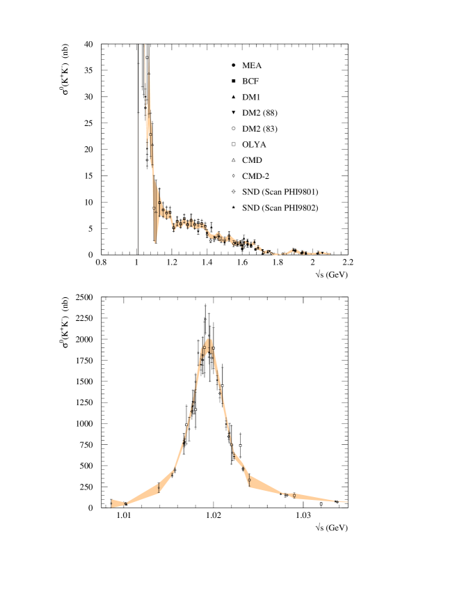
Figure 14: The data for $\sigma^{0}(e^{+}e^{-}\to K^{+}K^{-})$ together with an enlargement of the region of the $\phi$ resonance. The shaded band shows the result of our fit after clustering.

For the $K_{S}^{0}K_{L}^{0}$ channel, we use ten data sets [10, 14, 47, 48, 49], which also extend from 1.0 GeV to 2.1 GeV, see Fig. 15. Using the trapezoidal rule, the channel gives a contribution to the muon $g-2$ and $\Delta\alpha_{\rm had}$ of

$$a_{\mu}(K^{0}_{S}K^{0}_{L},\sqrt{s}<1.43~{}{\rm GeV},~{}{\rm data}) = (13.16\pm 0.31)\times 10^{-10},$$ (89)

$$\Delta\alpha_{\rm had}(K^{0}_{S}K^{0}_{L},\sqrt{s}<1.43~{}{\rm GeV},~{}{\rm data}) = (1.76\pm 0.04)\times 10^{-4}.$$ (90)

This channel is the one case where the use of the trapezoidal rule may overestimate the resonance contribution, due to the lack of data in certain regions of the $\phi$ resonance tails, see Fig. 15. We find that the use of a smooth resonance form in the tails decreases the contributions to $a_{\mu}$ and $\Delta\alpha_{\rm had}$ by about $0.15\times 10^{-10}$ and $0.02\times 10^{-4}$ respectively. We have therefore increased the error in (89) and (90) to include this additional uncertainty.

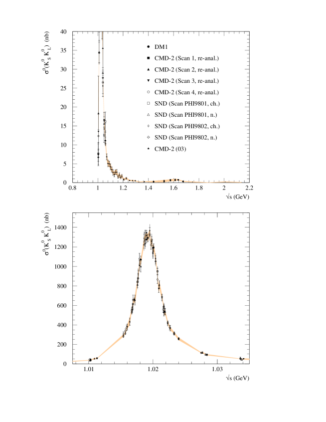
Figure 15: The data for $\sigma^{0}(e^{+}e^{-}\to K_{S}^{0}K_{L}^{0})$ together with an enlargement of the region of the $\phi$ resonance. The shaded band shows the result of our fit after clustering; however, the errors on the contribution of this channel to $a_{\mu}$ and $\Delta\alpha_{\rm had}$ are increased to allow for the lack of data in certain regions of the $\phi$ resonance tails, see the discussion in the text.

3.7 $K\bar{K}+n\pi$ contributions

We take into account the $K\bar{K}+n\pi$ final states for $n=1$ and 2.

For the $K\bar{K}\pi$, in addition to the data for the $K_{S}^{0}\pi^{\pm}K^{\mp}$ [74, 75, 76] and $K^{+}K^{-}\pi^{0}$ [74, 75] channels, we use the equalities $\sigma(K_{L}^{0}\pi K)=\sigma(K_{S}^{0}\pi K)$ and $\sigma(K_{S}^{0}K_{L}^{0}\pi^{0})=\sigma(K^{+}K^{-}\pi^{0})$, which follow directly from isospin. The contribution from the $K_{S}^{0}\pi^{\pm}K^{\mp}+K^{0}_{L}\pi^{\pm}K^{\mp}$ channel is

$$a_{\mu}(K_{S}^{0}\pi^{\pm}K^{\mp}+K^{0}_{L}\pi^{\pm}K^{\mp},\sqrt{s}<1.43~{}{\rm GeV},~{}{\rm data~{}and~{}isospin})=(0.10\pm 0.04)\times 10^{-10},$$ (91)

$$\Delta\alpha_{\rm had}(K_{S}^{0}\pi^{\pm}K^{\mp}+K^{0}_{L}\pi^{\pm}K^{\mp},\sqrt{s}<1.43~{}{\rm GeV},~{}{\rm data~{}and~{}isospin})=(0.02\pm 0.00)\times 10^{-4}.$$ (92)

For the $K^{+}K^{-}\pi^{0}+K^{0}_{S}K^{0}_{L}\pi^{0}$ channel, the contribution from the region $\sqrt{s}<1.43$ GeV is taken to be zero since the first data point is at 1.44 GeV.

To evaluate the $K\bar{K}\pi\pi$ contribution we use the inclusive data for $K_{S}X$ [77], together with the cross section relation

$$2K_{S}X = K_{S}X+K_{L}X$$ (93)

$$= 2K_{S}K_{L}+2(K_{S}K_{L}+K_{S}K_{S}+K_{L}K_{L})(\pi+\pi\pi)$$

$$\qquad\qquad\qquad\qquad\qquad\qquad+(K_{S}+K_{L})(K\pi+K\pi\pi),$$

where $2K_{S}X$ stands for 2$\sigma^{0}(e^{+}e^{-}\to K_{S}X)$ and similarly for the other abbreviations. On the right-hand-side $\pi\pi$ stands for $\pi^{+}\pi^{-}$ or $\pi^{0}\pi^{0}$, $K\pi$ for $K^{+}\pi^{-}$ or $K^{-}\pi^{+}$, and $K\pi\pi$ for $K^{+}\pi^{-}\pi^{0}$ or $K^{-}\pi^{+}\pi^{0}$. On the other hand, the $K\bar{K}\pi\pi$ cross section is given by

$$K\bar{K}\pi\pi = (K_{S}K_{L}+K_{S}K_{S}+K_{L}K_{L})(\pi\pi)+(K_{S}+K_{L})(K\pi\pi)+(K^{+}K^{-})(\pi\pi)$$ (94)

$$= 2K_{S}X-2K_{S}K_{L}-(K_{S}K_{L}+K_{S}K_{S}+K_{L}K_{L})(2\pi+\pi\pi)$$

$$\qquad\qquad\qquad\qquad\qquad\qquad\qquad-2K_{S}(K\pi)+(K^{+}K^{-})(\pi\pi)$$

$$= 2(K_{S}X-K_{S}K_{L}-K^{+}K^{-}\pi-K_{S}(K\pi)),$$

where to obtain the second equality we have used (93). In other words, the total $K\bar{K}\pi\pi$ contribution is obtained from twice the inclusive $K_{S}X$ cross section by subtracting the appropriate $K\bar{K}$ and $K\bar{K}\pi$ contributions. For this channel, the contribution from the region $\sqrt{s}<1.43$ GeV is also taken to be zero since the data of the $K_{S}^{0}X$ final state start from 1.44 GeV.

3.8 Unaccounted modes

We still have to take into account contributions from the reactions $e^{+}e^{-}\to\omega\pi^{0}$ and $e^{+}e^{-}\to\omega\pi^{+}\pi^{-}$, in which the $\omega$ decays radiatively into $\pi^{0}\gamma$. We used seven data sets for the $e^{+}e^{-}\to\omega\pi^{0}$ channel [22, 51, 53], [58]–[61], and three data sets [38, 69, 70] for the $e^{+}e^{-}\to\omega\pi^{+}\pi^{-}$ channel. Note that the contributions from the $\omega(\to\pi^{+}\pi^{-}\pi^{0})\pi^{0}$ and $\omega(\to\pi^{+}\pi^{-})\pi^{0}$ channels are already included as a part of the multi-pion channels. We therefore need simply to multiply the original cross section $\sigma(e^{+}e^{-}\to\omega\pi^{0})$ by the branching ratio $B(\omega\to\pi^{0}\gamma)=0.087$ [104]. The same comments apply for the $\omega\pi^{+}\pi^{-}$ channel. The two channels give contributions

$$a_{\mu}(\omega(\to\pi^{0}\gamma)\pi^{0},\sqrt{s}<1.43~{}{\rm GeV}) = (0.64\pm 0.02)\times 10^{-10},$$ (95)

$$\Delta\alpha_{\rm had}(\omega(\to\pi^{0}\gamma)\pi^{0},\sqrt{s}<1.43~{}{\rm GeV}) = (0.12\pm 0.00)\times 10^{-4},$$ (96)

and

$$a_{\mu}(\omega(\to\pi^{0}\gamma)\pi^{+}\pi^{-},\sqrt{s}<1.43~{}{\rm GeV}) = (0.01\pm 0.00)\times 10^{-10},$$ (97)

$$\Delta\alpha_{\rm had}(\omega(\to\pi^{0}\gamma)\pi^{+}\pi^{-},\sqrt{s}<1.43~{}{\rm GeV}) = (0.00\pm 0.00)\times 10^{-4},$$ (98)

respectively.

Purely neutral contributions from the direct decays of $\rho$ and $\omega$ to $\pi^{0}\pi^{0}\gamma$ can be safely neglected, as the branching fractions are of the order $5\times 10^{-5}$ and $7\times 10^{-5}$ respectively [104, 122, 123], and are suppressed compared to the decays into $\pi^{0}\gamma$.

For the $\phi$ resonance we have so far accounted for the $\phi\to K^{+}K^{-}$, $K_{S}^{0}K_{L}^{0}$, $3\pi$, $\eta\gamma$ and $\pi^{0}\gamma$ channels. Since the branching fractions of these final states add up to 99.8% [104], we must allow for the 0.2% from the remaining final states. To do this, we first note that the contribution to $a_{\mu}^{\rm had,LO}$ from the $K^{+}K^{-}$ channel in the $\phi$ region is

$$a_{\mu}(\phi\to K^{+}K^{-};2m_{K^{+}}<\sqrt{s}<1.03~{}{\rm GeV})=16.15\times 10^{-10}.$$ (99)

Using this, we estimate that the total contribution from the $\phi$ to be

$$a_{\mu}(\phi)=a_{\mu}(\phi\to K^{+}K^{-})/B(\phi\to K^{+}K^{-})=32\times 10^{-10}.$$

Hence we include the small residual contribution

$$a_{\mu}(\phi\to{\rm remaining~{}channels})=a_{\mu}(\phi)\times 0.002=0.06\times 10^{-10},$$ (100)

and assign to it a 100% error. In a similar way the contribution $\Delta\alpha_{\rm had}(\phi\to K^{+}K^{-})=2.12\times 10^{-4}$ is used to estimate

$$\Delta\alpha_{\rm had}(\phi\to{\rm remaining~{}channels})=0.01\times 10^{-4},$$ (101)

to which we again assign a 100% error.

3.9 Baryon-pair contribution

If we are to integrate up to high enough energy to pair-produce baryons, we have to take into account the $p\bar{p}$ and $n\bar{n}$ final states. The data come from the FENICE  [78, 79], DM1 [82] and DM2 [80, 81] collaborations for the $p\bar{p}$ channel, and from the FENICE collaboration [78, 83] for the $n\bar{n}$ channel. They do not contribute when we integrate over the exclusive channels only up to 1.43 GeV, but if we integrate up to 2.0 GeV, the $p\bar{p}$ channel gives a contribution of

$$a_{\mu}(p\bar{p},\sqrt{s}<2.0~{}{\rm GeV}) = (0.04\pm 0.01)\times 10^{-10},$$ (102)

$$\Delta\alpha_{\rm had}(p\bar{p},\sqrt{s}<2.0~{}{\rm GeV}) = (0.02\pm 0.00)\times 10^{-4},$$ (103)

while the $n\bar{n}$ channel gives

$$a_{\mu}(n\bar{n},\sqrt{s}<2.0~{}{\rm GeV}) = (0.07\pm 0.02)\times 10^{-10},$$ (104)

$$\Delta\alpha_{\rm had}(n\bar{n},\sqrt{s}<2.0~{}{\rm GeV}) = (0.03\pm 0.01)\times 10^{-4}.$$ (105)

3.10 Narrow resonance ($J/\psi,\psi^{\prime},\Upsilon$) contributions

We add the contributions from the narrow resonances, $J/\psi,\psi^{\prime}$ and $\Upsilon(1S-6S)$. We treat them in the zero-width approximation, in which the total production cross section of a vector meson $V$ $(V=J/\psi,\psi^{\prime},\Upsilon)$ is

$$\sigma(e^{+}e^{-}\to V)=12\pi^{2}\frac{\Gamma^{0}_{ee}}{M_{V}}\delta(s-M_{V}^{2}).$$ (106)

Here $\Gamma^{0}_{ee}$ is the bare leptonic width of $V$,

$$\Gamma^{0}_{ee}=C_{\rm res}\Gamma(V\to e^{+}e^{-}),$$ (107)

where

$$C_{\rm res}=\frac{(\alpha/\alpha(m_{V}^{2}))^{2}}{1+(3/4)\alpha/\pi},$$ (108)

which is about 0.95 for $J/\psi$ and $\psi^{\prime}$, and about 0.93 for the six $\Upsilon$ resonances [105]. We use the values compiled in RPP for the leptonic widths, $\Gamma(V\to e^{+}e^{-})$, and obtain the contributions

$$a_{\mu}(J/\psi) = (5.89\pm 0.41)\times 10^{-10},$$ (109)

$$a_{\mu}(\psi^{\prime}) = (1.41\pm 0.12)\times 10^{-10},$$ (110)

$$a_{\mu}(\Upsilon(1S)) = (0.05\pm 0.00)\times 10^{-10},$$ (111)

$$a_{\mu}(\Upsilon(2S-6S)) = (0.05\pm 0.00)\times 10^{-10},$$ (112)

and

$$\Delta\alpha_{\rm had}(J/\psi) = (6.65\pm 0.47)\times 10^{-4},$$ (113)

$$\Delta\alpha_{\rm had}(\psi^{\prime}) = (2.25\pm 0.19)\times 10^{-4},$$ (114)

$$\Delta\alpha_{\rm had}(\Upsilon(1S)) = (0.54\pm 0.02)\times 10^{-4},$$ (115)

$$\Delta\alpha_{\rm had}(\Upsilon(2S-6S)) = (0.62\pm 0.03)\times 10^{-4}.$$ (116)

3.11 Inclusive hadronic data contribution ($\sqrt{s}<11.09~{}{\rm GeV}$)

We use four data sets below 2 GeV [84]–[87], and twelve data sets above 2 GeV [88]–[98] (see Fig. 16). Below 2 GeV, we correct for the unaccounted modes. Namely, we add the contributions from the $\omega(\to\pi^{0}\gamma)\pi^{0}$ and $K_{S}^{0}(\to 2\pi^{0})K_{L}^{0}\pi^{0}$ channels to the experimentally observed $R$-ratio, since the final states of these channels consist only of electrically neutral particles, which are hard to see experimentally. They shift the $R$ values by roughly 1%, depending on $\sqrt{s}$. In addition we correct some experiments for the contributions from missing two-body final states, as discussed at the end of Section 2. We have also checked that corrections for $\gamma-Z$ interference effects are completely negligible in the energy range below 11.09 GeV where we use data.

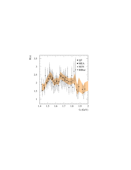
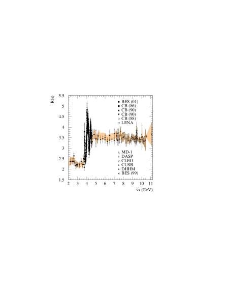
Figure 16: Data for the measurement of the inclusive hadronic cross section below 2 GeV (left) and above 2 GeV (right). The shaded band shows the behaviour of the hadronic $R$ ratio after clustering and fitting the data.

The contributions to the muon $g-2$ and $\Delta\alpha_{\rm had}$ are, from $1.43<\sqrt{s}<2$ GeV,

$$a_{\mu}({\rm inclusive},\sqrt{s}<2~{}{\rm GeV}) = (31.91\pm 2.42)\times 10^{-10},$$ (117)

$$\Delta\alpha_{\rm had}({\rm inclusive},\sqrt{s}<2~{}{\rm GeV}) = (10.78\pm 0.81)\times 10^{-4},$$ (118)

and from $2<\sqrt{s}<11.09$ GeV,

$$a_{\mu}({\rm inclusive},2<\sqrt{s}<11.09~{}{\rm GeV}) = (42.05\pm 1.14)\times 10^{-10},$$ (119)

$$\Delta\alpha_{\rm had}({\rm inclusive},2<\sqrt{s}<11.09~{}{\rm GeV}) = (81.97\pm 1.53)\times 10^{-4},$$ (120)

respectively.

3.12 Inclusive pQCD contribution ($\sqrt{s}>11.09~{}{\rm GeV}$)

Above 11 GeV we use perturbative QCD to evaluate the contributions to $a^{\rm had,LO}_{\mu}$ and $\Delta\alpha(M_{Z}^{2})$. We incorporate ${\cal O}(\alpha_{S}^{3})$ massless quark contributions, and the ${\cal O}(\alpha_{S}^{2})$ massive quark contributions [107, 124, 125, 126, 127]. We have checked that our code agrees very well with the code rhad written by Harlander and Steinhauser [128]. As input parameters, we use

$$\alpha_{S}(M_{Z}^{2})=0.1172\pm 0.002,~{}~{}~{}m_{t}=174.3\pm 5.1~{}{\rm GeV},~{}~{}~{}m_{b}=4.85\pm 0.25~{}{\rm GeV},$$ (121)

and allow for an uncertainty in the renormalization scale of $\sqrt{s}/2<\mu<2\sqrt{s}$. Here $m_{t}$ and $m_{b}$ are the pole masses of the top and bottom quark. We obtain

$$a_{\mu}({\rm pQCD},\sqrt{s}>11.09~{}{\rm GeV}) = (2.11\pm 0.00)\times 10^{-10},$$ (122)

where the uncertainty from $\alpha_{S}(M_{Z}^{2})$ is dominant, which is less than $1\times 10^{-12}$. Similarly, for $\Delta\alpha_{\rm had}$ we find

$$\Delta\alpha_{\rm had}({\rm pQCD},\sqrt{s}>11.09~{}{\rm GeV}) = (125.32\pm 0.14\pm 0.02\pm 0.01)\times 10^{-4}$$ (123)

$$= (125.32\pm 0.15)\times 10^{-4},$$ (124)

where the first error comes from the uncertainty in $\alpha_{S}(M_{Z}^{2})$, the second from the renormalization scale $\mu$, and the third from that on the mass of the bottom quark.

3.13 Total contribution to the dispersion integrals

To summarize, Table 5 shows the values obtained for $a_{\mu}^{\rm had,LO}$ and $\Delta\alpha_{\rm had}$, as well as showing the contributions of the individual channels. Summing all the contributions we obtain

$$a_{\mu}^{\rm had,LO}({\rm incl.}) = (692.38\pm 5.88_{\rm exp})\times 10^{-10},$$ (125)

$$a_{\mu}^{\rm had,LO}({\rm excl.}) = (696.15\pm 5.68_{\rm exp})\times 10^{-10},$$ (126)

where “incl.” means that we have used the inclusive data sets for $1.43<\sqrt{s}<2~{}{\rm GeV}$, while “excl.” means that we used the exclusive data at the same interval. “exp.” means that the errors are from the experimental uncertainty. The corresponding results for $\Delta\alpha_{\rm had}$ are

$$\Delta\alpha_{\rm had}({\rm incl.}) = (275.52\pm 1.85_{\rm exp})\times 10^{-4},$$ (127)

$$\Delta\alpha_{\rm had}({\rm excl.}) = (276.90\pm 1.77_{\rm exp})\times 10^{-4}.$$ (128)

We see that using the sum of the data for exclusive channels to determine $R(s)$, in the intermediate energy interval $1.43<\sqrt{s}<2~{}{\rm GeV}$, yields values for $a_{\mu}^{\rm had,LO}$ and $\Delta\alpha_{\rm had}$ which significantly exceed the values obtained using the inclusive data for $R(s)$. The mean values differ by about $2/3$ of the total experimental error. In Fig. 17 we show the hadronic $R$ ratio as a function of $\sqrt{s}$. A careful inspection of the figure shows the discrepancy between the inclusive and exclusive data sets in the interval $1.43<\sqrt{s}<2~{}{\rm GeV}$, see Fig. 4. The contribution from this region alone is

$$a_{\mu}^{\rm had,LO}(1.43<\sqrt{s}<2~{}{\rm GeV},{\rm~{}incl.}) = (31.91\pm 2.42_{\rm exp})\times 10^{-10},$$ (129)

$$a_{\mu}^{\rm had,LO}(1.43<\sqrt{s}<2~{}{\rm GeV},{\rm~{}excl.}) = (35.68\pm 1.71_{\rm exp})\times 10^{-10},$$ (130)

and for $\Delta\alpha_{\rm had}$,

$$\Delta\alpha_{\rm had}(1.43<\sqrt{s}<2~{}{\rm GeV},{\rm~{}incl.}) = (10.78\pm 0.81_{\rm exp})\times 10^{-4},$$ (131)

$$\Delta\alpha_{\rm had}(1.43<\sqrt{s}<2~{}{\rm GeV},{\rm~{}excl.}) = (12.17\pm 0.59_{\rm exp})\times 10^{-4}.$$ (132)

In the next Section we introduce QCD sum rules that are able to determine which choice of $R(s)$ is consistent. We find that the sum rules strongly favour the use of the inclusive data in the above intermediate energy interval.

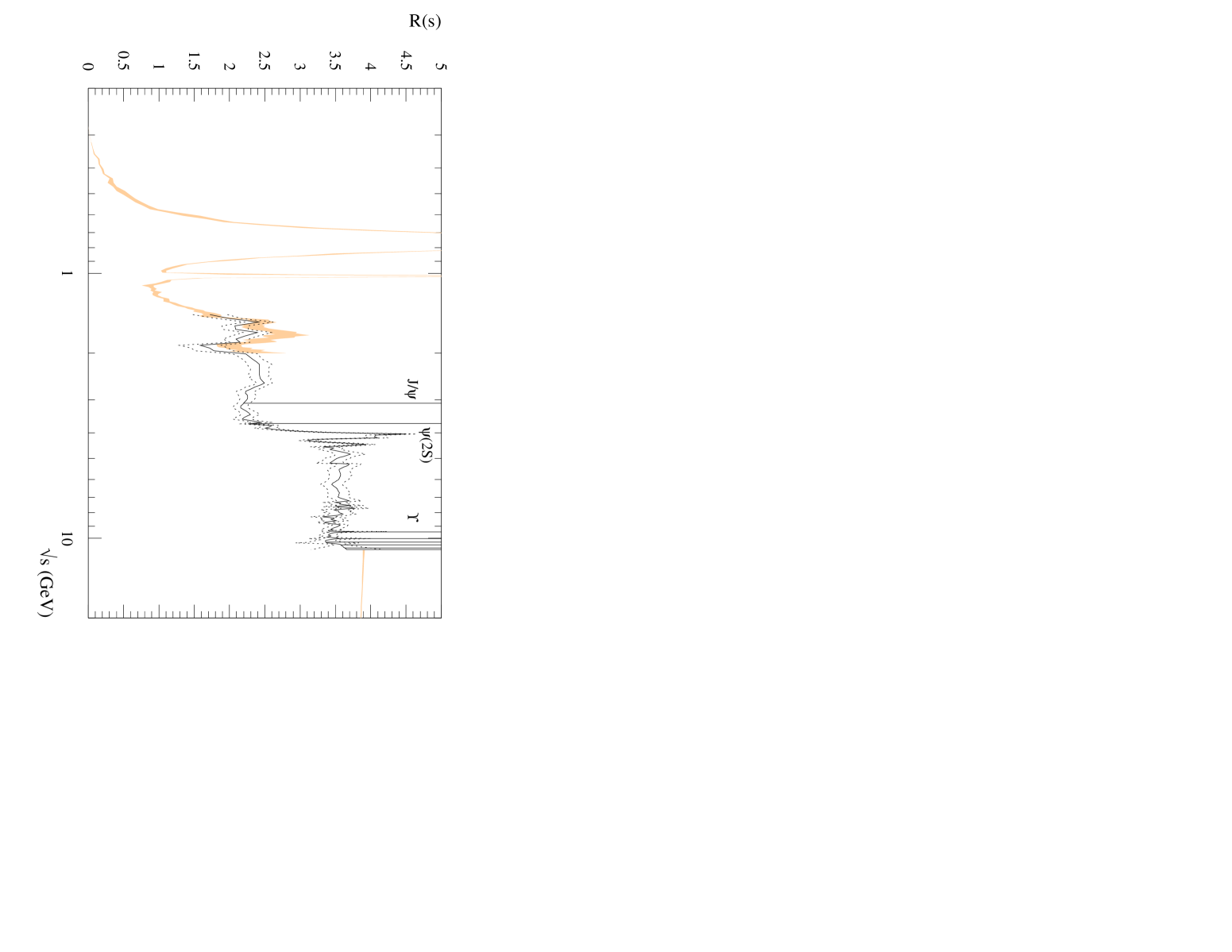
Figure 17: The hadronic $R$ ratio as a function of $\sqrt{s}$. Note that the values of $R$ obtained from the sum of the exclusive channels and from the inclusive data overlap in the region $1.4\mathop{}_{\textstyle\sim}^{\textstyle<}\sqrt{s}\mathop{}_{\textstyle\sim}^{\textstyle<}2$ GeV.

Table 7 shows the breakdown of the contributions versus energy. It is also useful to show the breakdown visually in terms of ‘pie’ diagrams.

energy range (GeV)	comments	$a^{\rm had,LO}_{\mu}\times 10^{10}$	$\Delta\alpha_{\rm had}(M_{Z}^{2})\times 10^{4}$
$m_{\pi}$–0.32	ChPT	$2.36\pm 0.05$	$0.04\pm 0.00$
0.32–1.43	excl. only	$606.55\pm 5.22$	$47.34\pm 0.35$
1.43–2	incl. only	$31.91\pm 2.42$	$10.78\pm 0.81$
	(excl. only	$35.68\pm 1.71$	$12.17\pm 0.59$)
2–11.09	incl. only	$42.05\pm 1.14$	$81.97\pm 1.53$
$J/\psi$ and $\psi^{\prime}$	narrow width	$7.30\pm 0.43$	$8.90\pm 0.51$
$\Upsilon(1S-6S)$	narrow width	$0.10\pm 0.00$	$1.16\pm 0.04$
11.09–$\infty$	pQCD	$2.11\pm 0.00$	$125.32\pm 0.15$
Sum of all	incl. 1.43–2	$692.38\pm 5.88$	$275.52\pm 1.85$
	(excl. 1.43–2	$696.15\pm 5.68$	$276.90\pm 1.77$)

Table 7: A breakdown of the contributions to different intervals of the dispersion integrals for $a_{\mu}^{\rm had,LO}$ and $\Delta\alpha_{\rm had}(M_{Z}^{2})$. The alternative numbers for the interval $1.43<\sqrt{s}<2$ GeV correspond to using data for either the sum of the exclusive channels or the inclusive measurements, see Fig. 4.

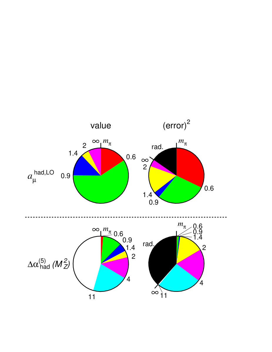
Figure 18: The pie diagrams in the left- and right-hand columns show the fractions of the total contributions and $({\rm errors})^{2}$, respectively, coming from various energy intervals in the dispersion integrals (4) and (5). The pie diagrams for the LO hadronic contribution to $g-2$, shown in the first row, correspond to sub-contributions with energy boundaries at $m_{\pi},0.6,0.9,1.4,2~{}{\rm GeV}{\rm~{}and}~{}\infty$, whereas for the hadronic contribution to the QED coupling, shown in the second row, the boundaries are at $m_{\pi},0.6,0.9,1.4,2,4,11.09~{}{\rm GeV}{\rm~{}and}~{}\infty$. In the $({\rm error})^{2}$ pie diagrams we also included the $({\rm error})^{2}$ arising from the treatment of the radiative corrections to the data.

The ‘pie’ diagrams on the left-hand side of Fig. 18 show the fraction of the total contributions to $a_{\mu}^{\rm had,LO}$ and $\Delta\alpha_{\rm had}$ coming from various energy intervals of the dispersion integrals (4) and (5). The plots on the right-hand-side indicate the fractional contributions to the square of the total error, including the error due to the treatment of radiative corrections. The values shown for $a_{\mu}^{\rm had,LO}$ in these plots correspond to using the inclusive data in the intermediate energy interval.

In Section 7 we use the value of $a_{\mu}^{\rm had,LO}$, along with the QED, weak and other hadronic contributions, to predict the value of $g-2$ of the muon. In Section 8 we use the value of $\Delta\alpha_{\rm had}(M_{Z}^{2})$ to predict the value of the QED coupling on the $Z$ pole, $\alpha(M_{Z}^{2})$.

4 Resolution of the ambiguity: QCD sum rules

To decide between the exclusive and inclusive data in the energy range $1.43<\sqrt{s}<2$ GeV (see Fig. 4), we make use of QCD sum rules [129], see also the review [130]. The sum rules are based on the analyticity of the vacuum polarization function $\Pi(q^{2})$, from which it follows that a relation of the form

$$\int_{s_{\rm th}}^{s_{0}}\ {\rm d}s\ R(s)f(s)\ =\ \int_{C}\ {\rm d}s\ D(s)g(s)$$ (133)

must be satisfied for a non-singular function $f(s)$. $C$ is a circular contour of radius $s_{0}$ and $g(s)$ is a known function once $f(s)$ is given. The lower limit of integration, $s_{\rm th}$, is $4m_{\pi}^{2}$, except for a small $e^{+}e^{-}\to\pi^{0}\gamma$ contribution. $D(s)$ is the Adler $D$ function,

$$D(s)\ \equiv\ -12\pi^{2}s\frac{{\rm d}}{{\rm d}s}\left(\frac{\Pi(s)}{s}\right),\qquad{\rm where}\quad R(s)\ =\ \frac{12\pi}{s}\,{\rm Im}\,\Pi(s).$$ (134)

Provided that $s_{0}$ is chosen sufficiently large for $D(s)$ to be evaluated from QCD, the sum rules allow consistency checks of the behaviour of the data for $R(s)$ for $s<s_{0}$. Indeed, by choosing an appropriate form of the function $f(s)$ we can highlight the average behaviour of $R(s)$ over a particular energy domain. To be specific, we take $s_{0}$ just below the open charm threshold (say $\sqrt{s}_{0}=3.7\ {\rm GeV}$) and choose forms for $f(s)$ which emphasize the most ambiguous range ($1.5\;\raisebox{-3.01385pt}{$\stackrel{{\scriptstyle\textstyle<}}{{\sim}}$}\;\sqrt{s}\;\raisebox{-3.01385pt}{$\stackrel{{\scriptstyle\textstyle<}}{{\sim}}$}\;2$ GeV) of $R(s)$, so that the discriminating power of the sum rules is maximized. We therefore use the three flavour ($n_{f}=3$) QCD expressions for $D(s)$, and omit the $J/\psi$ and $\psi(2S)$ $c\bar{c}$ resonance contributions to $R(s)$.

To evaluate the function $D(s)$ from QCD, it is convenient to express it as the sum of three contributions,

$$D(s)\ =\ D_{0}(s)+D_{\rm m}(s)+D_{\rm np}(s),$$ (135)

where $D_{0}$ is the $O(\alpha_{S}^{3})$ massless, three-flavour QCD prediction, $D_{\rm m}$ is the (small) quark mass correction and $D_{\rm np}$ is a (very small) contribution estimated using knowledge of the condensates. $D_{0}$ is given by [124]

$$D_{0}(-s)=3\sum_{f}Q_{f}^{2}\left\{1+\frac{\alpha_{S}(s)}{\pi}+d_{1}\left(\frac{\alpha_{S}(s)}{\pi}\right)^{2}+\tilde{d}_{2}\left(\frac{\alpha_{S}(s)}{\pi}\right)^{3}+{\cal O}\left(\alpha_{S}^{4}(s)\right)\right\},$$ (136)

with

$$d_{1} = 1.9857-0.1153n_{f},$$ (137)

$$\tilde{d}_{2} = d_{2}+\frac{\beta_{0}^{2}\pi^{2}}{48}~{}~{}~{}~{}~{}\left({\rm with\ }\beta_{0}=11-\frac{2n_{f}}{3}\right),$$ (138)

$$d_{2} = -6.6368-1.2001n_{f}-0.0052n_{f}^{2}-1.2395\frac{(\sum_{f}Q_{f})^{2}}{3\sum_{f}Q_{f}^{2}},$$ (139)

where the sum $f$ runs over $u,d$ and $s$ flavours. $Q_{f}$ is the electric charge of quark $f$, which takes the values 2/3, $-1/3$, and $-1/3$ for $u,d$ and $s$, respectively. The quark mass correction $D_{\rm m}$ reads [131]

$$D_{\rm m}(-s)=-3\sum_{f}Q_{f}^{2}\frac{m_{f}^{2}(s)}{s}\left(6+28\frac{\alpha_{S}(s)}{\pi}+(294.8-12.3n_{f})\left(\frac{\alpha_{S}(s)}{\pi}\right)^{2}\right).$$ (140)

We take the $\overline{\rm MS}$ $s$-quark mass at 2 GeV $m_{s}(4~{}{\rm GeV}^{2})$ to be $120\pm 40$ MeV, and we neglect the $u$ and $d$ quark masses. The contribution from condensates, $D_{\rm np}$, is given by

$$D_{\rm np}(-s) = 3\sum_{f}Q_{f}^{2}\left\{\frac{2\pi^{2}}{3}\left(1-\frac{11}{18}\frac{\alpha_{S}(s)}{\pi}\right)\frac{\langle(\alpha_{S}/\pi)GG\rangle}{s^{2}}\right.$$ (141)

$$\phantom{3\sum_{f}Q_{f}^{2}}+8\pi^{2}\left(1-\frac{\alpha_{S}(s)}{\pi}\right)\frac{\langle m_{f}\overline{q}_{f}q_{f}\rangle}{s^{2}}+\frac{32\pi^{2}}{27}\frac{\alpha_{S}(s)}{\pi}\sum_{k}\frac{\langle m_{k}\overline{q}_{k}q_{k}\rangle}{s^{2}}$$

$$\left.\phantom{3\sum_{f}Q_{f}^{2}}+12\pi^{2}\frac{\langle{\cal O}_{6}\rangle}{s^{3}}+16\pi^{2}\frac{\langle{\cal O}_{8}\rangle}{s^{4}}\right\},$$

where, following [132], we take

$$\left\langle\frac{\alpha_{S}}{\pi}GG\right\rangle = 0.037\pm 0.019\ ({\rm GeV}^{4}),$$

$$\langle m_{s}\bar{s}s\rangle = -f_{\pi}^{2}m_{K}^{2}.$$ (142)

Here $f_{\pi}\simeq 92$ MeV is the pion decay constant, and $m_{K}$ is the kaon mass. As we will see later, the quark mass corrections and the condensate contributions are very tiny—typically at most a few percent of the whole QCD contribution. Hence we neglect the higher dimensional condensates, $\langle{\cal O}_{6}\rangle$ and $\langle{\cal O}_{8}\rangle$.

As for the weight function $f(s)$, we take it to be of the form $(1-s/s_{0})^{m}(s/s_{0})^{n}$ with $n+m=0,1$ or $2$. For these six choices of $f(s)$, the function $g(s)$ may be readily evaluated, and the sum rules, (133), become

$$\int_{s_{\rm th}}^{s_{0}}{\rm d}sR(s) = \frac{i}{2\pi}\int_{C}{\rm d}s\left\{1-\frac{s_{0}}{s}\right\}D(s),$$ (143)

$$\int_{s_{\rm th}}^{s_{0}}{\rm d}sR(s)\frac{s}{s_{0}} = \frac{i}{2\pi}\int_{C}{\rm d}s\frac{1}{2}\left\{\frac{s}{s_{0}}-\frac{s_{0}}{s}\right\}D(s),$$ (144)

$$\int_{s_{\rm th}}^{s_{0}}{\rm d}sR(s)\left(1-\frac{s}{s_{0}}\right) = \frac{i}{2\pi}\int_{C}{\rm d}s\left\{-\frac{1}{2}\frac{s}{s_{0}}+1-\frac{1}{2}\frac{s_{0}}{s}\right\}D(s),$$ (145)

$$\int_{s_{\rm th}}^{s_{0}}{\rm d}sR(s)\left(\frac{s}{s_{0}}\right)^{2} = \frac{i}{2\pi}\int_{C}{\rm d}s\frac{1}{3}\left\{\left(\frac{s}{s_{0}}\right)^{2}-\frac{s_{0}}{s}\right\}D(s),$$ (146)

$$\int_{s_{\rm th}}^{s_{0}}{\rm d}sR(s)\left(1-\frac{s}{s_{0}}\right)\frac{s}{s_{0}} = \frac{i}{2\pi}\int_{C}{\rm d}s\left\{-\frac{1}{3}\left(\frac{s}{s_{0}}\right)^{2}+\frac{1}{2}\frac{s}{s_{0}}-\frac{1}{6}\frac{s_{0}}{s}\right\}D(s),$$ (147)

$$\int_{s_{\rm th}}^{s_{0}}{\rm d}sR(s)\left(1-\frac{s}{s_{0}}\right)^{2} = \frac{i}{2\pi}\int_{C}{\rm d}s\left\{\frac{1}{3}\left(\frac{s}{s_{0}}\right)^{2}-\frac{s}{s_{0}}+1-\frac{1}{3}\frac{s_{0}}{s}\right\}D(s).$$ (148)

We evaluate each of these sum rules for $\sqrt{s_{0}}=3.7$ GeV using the clustered data values of $R(s)$ of Section 2 on the l.h.s., and QCD for $D(s)$ (with $\alpha_{S}=0.1172\pm 0.0020$ [104]) on the r.h.s. We find, as anticipated, that the sum rules with $m=0$ and $n=1$ or 2 have very small contributions from the disputed 1.43—2 GeV region. Indeed, this region contributes only about 5% and 2%, respectively, of the total contribution to the l.h.s. of (144) and (146). They emphasize the region $s\;\raisebox{-3.01385pt}{$\stackrel{{\scriptstyle\textstyle<}}{{\sim}}$}\;s_{0}$ and so essentially test data against perturbative QCD in this small domain. They are not useful for our purpose. The results for the remaining four sum rules are shown by the numbers in brackets in Fig. 19. For this choice of $s_{0}$, the sum rules with $m=1$ or 2 and $n=0$ are found to maximize the fractional contribution to the sum rule coming from the $1.43<\sqrt{s}<2$ GeV interval. These two sum rules clearly favour the inclusive over the exclusive data.

(a) Breakdown of contributions to l.h.s. of sum rules
energy range (GeV)	contribution ($m=2,n=0$)	contribution ($m=n=0$)
$2m_{\pi}-0.32$ (ChPT)	0.00 $\pm$ 0.00	0.00 $\pm$ 0.00
$0.32-1.43$ (excl)	3.92 $\pm$ 0.03	4.49 $\pm$ 0.04
$1.43-2.00$ (excl)	3.02 $\pm$ 0.26	4.93 $\pm$ 0.43
$1.43-2.00$ (incl)	2.48 $\pm$ 0.19	4.03 $\pm$ 0.30
$2.00-3.73$ (incl)	3.94 $\pm$ 0.14	22.56 $\pm$ 0.70
sum (excl)	10.87 $\pm$ 0.30	31.98 $\pm$ 0.82
sum (incl)	10.34 $\pm$ 0.24	31.08 $\pm$ 0.76

(b) Breakdown of contributions to r.h.s. of sum rules
origin	contribution ($m=2,n=0$)	contribution ($m=n=0$)
massless QCD	10.31 $\pm$ 0.05	30.43 $\pm$ 0.11
correction from finite $m_{s}$	$-0.03$ $\pm$ 0.02	$-0.03\pm 0.02$
quark and gluon condensates	0.03 $\pm$ 0.02	0.00 $\pm$ 0.00
prediction from QCD (total)	10.30 $\pm$ 0.06	30.40 $\pm$ 0.12

Table 8: The breakdown of the sum rules for $\sqrt{s_{0}}=3.7$ GeV, for the choices $m=2,n=0$ and $m=n=0$. The contributions to the left-hand-side (data) are shown in the upper table, and the QCD contributions are given in the lower table.

The comparison between the data and QCD can be translated into another form. We can treat $\alpha_{S}(M_{Z}^{2})$ as a free parameter, and calculate the value which makes the r.h.s. of a sum rule exactly balance the l.h.s. The results are shown in Fig. 19. We can see that in this comparison the determination from the inclusive data is more consistent with the world-average value, $\alpha_{S}(M_{Z}^{2})=0.1172\pm 0.0020$ [104].

For illustration, we show in Table 8 a detailed breakdown of the contributions to both sides of the sum rule for the cases of $m=2,n=0$ and $m=n=0$. If we compare the breakdown of the contribution from the data in both cases, we can see that the weight function $f(s)=(1-s/s_{0})^{2}$ highlights the most ambiguous region of $R(s)$ very well. When we look into the breakdown in the QCD part, we can see that the QCD contribution is dominated by the massless part.

We repeated the sum rule analysis for $\sqrt{s_{0}}=3.0$ GeV, see Fig. 19. The lower value of $s_{0}$ means that more weight is given to the disputed 1.43—2 GeV region. Taken together, we see that the sum rules strongly favour the behaviour of $R(s)$ from the inclusive measurements. Indeed, the overall consistency in this case is remarkable. This result can also be clearly seen from Fig. 19, which compares the world average value of $\alpha_{S}(M_{Z}^{2})$ with the predictions of the individual sum rules for, first $\sqrt{s_{0}}=3.7$ GeV and then for $\sqrt{s_{0}}=3$ GeV. Again the consistency with the inclusive measurements of $R(s)$ is apparent.

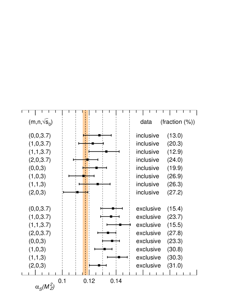
Figure 19: The QCD sum rule predictions for $\alpha_{S}(M_{Z}^{2})$ compared with the world average value [104]. The results for the four sum rules for two values of $\sqrt{s_{0}}$ are shown. In each case we show results for the inclusive and the exclusive measurement of $R(s)$ in the intermediate energy region. We also give in brackets the fractional contribution to the sum rule coming from the $1.43<\sqrt{s}<2$ GeV interval.

The same conclusion with regard to the resolution of the inclusive/exclusive ambiguity in the $1.43<\sqrt{s}<2$ GeV interval was reached in an independent analysis [133].

In an attempt to understand the origin of the discrepancy, we have studied the effect of possibly missing (purely neutral) modes in the inclusive data, but found that these cannot explain the difference. One should, however, keep in mind that the precision of both the (old) inclusive and the exclusive data in this energy regime is quite poor. We expect that future measurements at $B$-factories (via radiative return) and at the upgraded machine VEPP-2000 in Novosibirsk will improve the situation in the future.

5 Comparison with other predictions of $g-2$

Fig. 20 shows other determinations of $a^{\rm had,LO}_{\mu}$, together with the values (HMNT(03)) obtained in this work. The values listed below the first dashed line incorporate the new more precise data on $e^{+}e^{-}\to\pi^{+}\pi^{-}$ [11] into the analysis. These data play a dominant role, and, as can be seen from the Figure, significantly decrease the value of $a_{\mu}^{\rm had}$. However, very recently, the CMD-2 Collaboration have re-analysed their data and found that they should be increased by approximately 2%, depending on $\sqrt{s}$. The new data [10] are included in our analysis. Inspection of Fig. 20 shows that the re-analysis of the CMD-2 data has led to an increase of $a_{\mu}^{\rm had,LO}\times 10^{10}$ by about 10.

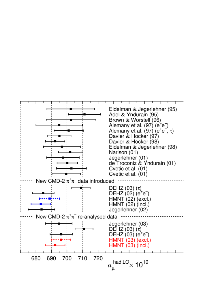
Figure 20: Recent evaluations of $a_{\mu}^{\rm had,LO}$ [2, 3, 12, 108, 132, 165, 166, 167, 168]. The entries below the first dashed line include the new CMD-2 $\pi^{+}\pi^{-}$ data [11], and the values below the second dashed line include the re-analysed CMD-2 $\pi^{+}\pi^{-}$ data [10].

The entries denoted by “DEHZ ($\tau$)” also used information from hadronic $\tau$ decays [2, 3], which through CVC give independent information on the $e^{+}e^{-}\to 2\pi$ and $4\pi$ channels for $\sqrt{s}\;\raisebox{-3.01385pt}{$\stackrel{{\scriptstyle\textstyle<}}{{\sim}}$}\;m_{\tau}$. The apparent discrepancy between the prediction from this analysis and the pure $e^{+}e^{-}$ analyses is not yet totally understood, however see the remarks in the Introduction.

5.1 Comparison with the DEHZ evaluation

It is particularly informative to compare the individual contributions to $a^{\rm had,LO}_{\mu}$ obtained in the present analysis with those listed in the recent study of Davier et al. (DEHZ03) [3], which used essentially the same $e^{+}e^{-}\to{\rm hadrons}$ data. Such a comparison highlights regions of uncertainty, and indicates areas where further data and study could significantly improve the theoretical determination of $g-2$. DEHZ provided a detailed breakdown of their contributions to $a^{\rm had,LO}_{\mu}$, and so, to facilitate the comparison, we have broken down our contributions into the energy intervals that they use. Table 9 shows the two sets of contributions of the individual $e^{+}e^{-}$ channels to dispersion relation (44) in the crucial low energy region with $\sqrt{s}<1.8$ GeV.

The last column of Table 9 shows the discrepancy between the two analyses. The biggest difference occurs in the $\pi^{+}\pi^{-}$ channel, which gives the main contribution to $a_{\mu}^{\rm had,LO}$, and the improvement in the SM prediction essentially comes from the recent higher precision CMD-2 data in the region $0.6<\sqrt{s}<0.9$ GeV (see the remarks in Chapter 3.2). We find that this difference, $2.6\times 10^{-10}$, appears to come from the region just above the $\pi^{+}\pi^{-}$ threshold, especially in the region $\sqrt{s}\sim 0.4$ GeV, see Fig. 21.

Figure 21: The $\pi^{+}\pi^{-}$ data just above threshold, plotted so that the area gives the contribution to dispersion relation (44) for $a_{\mu}^{\rm had,LO}$. The dashed curve is used by DEHZ [2, 3], whereas the continuous curve up to $\sqrt{s}=0.32$ GeV ($s=0.10$ GeV²) and data band are used in this analysis; see text. We also show, but do not use, the preliminary low energy CMD-2 data, which were read off Fig. 3 of [134]. These points, particularly the first, are subject to ‘reading-off’ errors.

The figure shows the $\pi^{+}\pi^{-}$ contribution plotted in such a way that the area under the curves (or data band) gives the contribution to dispersion relation (44) for $a_{\mu}^{\rm had,LO}$. To determine the low energy $\pi^{+}\pi^{-}$ contribution, DEHZ [2] first perform a three-parameter fit to $\pi^{+}\pi^{-}$ data for $\sqrt{s}<0.6$ GeV, and obtain the dashed curve in Fig. 21. This is then used to compute the $\pi^{+}\pi^{-}$ contribution of $(58.04\pm 2.06)\times 10^{-10}$ for $\sqrt{s}<0.5$ GeV. They do not use either the NA7 [20] or the preliminary CMD-2 data. On the other hand we use the chiral description [136], shown by the continuous curve, only as far as $\sqrt{s}=0.32$ GeV; and then use the band obtained from our clustered data, which include data from OLYA [16], TOF [19], NA7 [20], CMD [21] and DM1 [23] in this energy region. In this way we obtain a $\pi^{+}\pi^{-}$ contribution for $\sqrt{s}<0.5$ GeV of $(55.7\pm 1.9)\times 10^{-10}$. We also show on Fig. 21 the preliminary CMD-2 data, obtained from Fig. 3 of Ref. [134]. These data were used in neither analysis, but do seem to favour the lower $\pi^{+}\pi^{-}$ contribution. It is also interesting to note that DEHZ [2, 3] obtain the low value of $(56.0\pm 1.6)\times 10^{-10}$ if $\tau$ decay and CVC are used in this region.

Other significant, with respect to the errors, discrepancies arise in the $\pi^{0}\gamma+\eta\gamma$ and the $K^{0}_{S}K^{0}_{L}$ channels, where the treatment is different: DEHZ integrate over Breit–Wigner resonance parametrizations (assuming that the $KK$ channels are saturated by the $\phi$ decay), while we are integrating the available data in these channels directly. In our method there is no danger to omit or double-count interference effects and resonance contributions from tails still present at continuum energies, and the error estimate is straight forward. As a check, we made fits to Breit–Wigner-type resonance forms and studied the possibility that trapezoidal integration of concave structures overestimate the resonance contributions. We found the possible effects are negligible compared to the uncertainties in the parametrization coming from poor quality data in the tail regions. The one exception is the $\phi\to K_{S}^{0}K_{L}^{0}$ contribution. Here the lack of data in certain regions of the resonance tails (see Fig. 15) has caused us to increase the uncertainty on this contribution to $a_{\mu}$, see Section 3.6.

Apart from these channels, it is only the two four-pion channels which show uncomfortably large and relevant discrepancies. Here, the data input is different between DEHZ and our analysis. We use, in addition to DEHZ, also data from $\gamma\gamma 2$ [56, 66] and ORSAY-ACO [55] for both $4\pi$ channels, and data from M3N [50] and two more data sets from CMD-2 [67, 68] for the $\pi^{+}\pi^{-}\pi^{+}\pi^{-}$ channel. However, it should be noted, that the available data are not entirely consistent, a fact reflected in the poor $\chi^{2}_{\rm min}/{\rm d.o.f.}$ of our fits resulting in the need of error inflation. Clearly, in these channels, new and better data is required. As mentioned already in Section 3.5, the situation is expected to improve as soon as the announced re-analysis from CMD-2 will become available.

There are no data available for some of the exclusive channels. Their contribution to the dispersion relation is computed using isospin relations. The corresponding entries in Table 9 have been marked by the word “isospin”.

5.2 Possible contribution of the $\sigma(600)$ resonance to $g-2$

This subsection is motivated by the claim [137] that the isosinglet scalar boson $\sigma(600)$ can have a non-negligible contribution to the muon $g-2$. Here, we evaluate its contribution and find that it is at most of order $0.1\times 10^{-10}$. This is negligible as compared to the uncertainty of the hadronic vacuum polarization contribution of $6\times 10^{-10}$, and hence we can safely neglect it.

The argument presented in Ref. [137] is twofold. First $\sigma$ may contribute to the muon $g-2$ through unaccounted decay modes of the narrow spin 1 resonances into the $\sigma\gamma$ channel. The second possibility, considered in [137], is that $\sigma$ may contribute directly to the muon $g-2$ through its coupling to the muon pair. We estimate the two contributions below.

In the zero-width limit, narrow spin 1 resonances, $V$, contribute to the muon $g-2$ as

$$a_{\mu}^{V}=(3/\pi)K(m_{V}^{2})\Gamma(V\to ee)/m_{V},$$ (149)

where $K(m_{V}^{2})$ is the kernel function (45) at $s=m_{V}^{2}$. We find, for example,

$$a_{\mu}^{\omega}=391\times 10^{-10},$$ (150)

$$a_{\mu}^{\phi}=39\times 10^{-10},$$ (151)

$$a_{\mu}^{\phi(1.68)}=3.4\times 10^{-10},$$ (152)

where, in (152), we have used $\Gamma(\phi(1.68)\to ee)=0.48$ keV [104] to give a rough estimate. If the decays $V\to\sigma\gamma$ of the above vector bosons escape detection, a fraction of the above contributions up to $B(V\to\sigma\gamma)$ may have been missed. On the other hand we find that 99.8% of $\phi$ decays has been accounted for in the five decay channels explicitly included in our analysis hence $B(\phi\to\sigma\gamma)<0.002$. This severely constrains the $\sigma\gamma\gamma$ coupling. Hence we can use the Vector Meson Dominance (VMD) approximation to show that the other branching fractions satisfy $B(\omega\to\sigma\gamma)<7.2\times 10^{-5}$ and $B(\phi(1.68)\to\sigma\gamma)<3.5\times 10^{-5}$, see Appendix B. By inserting these constraints into the estimates (150)–(152), we find that the unaccounted $V\to\sigma\gamma$ contributions to $g-2$ of the muon are less than $(2.8,\,7.8,\,0.01)\times 10^{-12}$ for $V=\omega,\ \phi,\ \phi(1.68)$ respectively, assuming $m_{\sigma}=600$ MeV. These estimates are much smaller than those presented in [137]. It is clear that the total contribution of unaccounted $\sigma\gamma$ modes through narrow resonance decays is negligibly small. It is also worth pointing out here that the unaccounted fraction $0.2\%$ of the $\phi$ contribution ($7.8\times 10^{-12}$ above) has been taken into account in our analysis, whether it is $\phi\to\sigma\gamma$ or not.

We now turn to the $\sigma$ contribution to the muon $g-2$ through its direct coupling to a muon-pair. To evaluate this, it is essential to estimate the magnitude of the $\sigma\mu\mu$ coupling. Since the coupling through the $\sigma$-Higgs boson mixing is negligibly small, the leading contribution should come from two-photon exchange. In this regard, the effective coupling strength should be of the same order as that of the $\eta$ isoscalar pseudoscalar meson, which should also be dominated by the two-photon exchange. By using the observed width $\Gamma(\eta\to\mu\mu)$, and by neglecting the form factor suppression, we find that the point-like $\eta$ contribution to the muon $g-2$ is

$$a_{\mu}^{\eta}=-3\times 10^{-13},$$ (153)

which is negligibly small. It follows that this implies that $a_{\mu}^{\sigma}$ is also negligibly small, see (164) below. However, the discussion can be made far more general. It is presented in the next Section.

6 Internal light-by-light contributions

In this section we present a very primitive discussion of the hadronic contribution to the internal light-by-light amplitudes, motivated by the study of the direct $\sigma$ and $\eta$ contributions to the muon $g-2$.

The meaning of ‘internal’ can be seen from Fig. 22. We call the diagram on the right ‘internal’ to distinguish it from the left diagram, that is the familiar light-by-light contribution which, here, we call ‘external’. We should note that the external light-by-light diagram is of ${\cal O}(\alpha^{3})$ and the internal light-by-light diagram is an ${\cal O}(\alpha^{4})$ contribution.

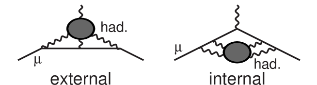
Figure 22: External and internal light-by-light contributions to $g-2$. The former is an ${\cal O}(\alpha^{3})$ and the latter is an ${\cal O}(\alpha^{4})$ contribution. In this paper we compute the contribution of the internal diagram. In Section 6.1 we take the shaded blob to be scalar ($\sigma$) or pseudoscalar ($\pi^{0},\eta$) mesons, whereas in Section 6.2 we take it to be a light ($u,d,s$) quark loop, using the result for lepton ($e,\mu$) loops as a guide.

6.1 Internal meson contributions

Just like the external light-by-light amplitude is dominated by a single pseudoscalar meson contribution [138]–[141], it is likely that the hadronic contribution to the internal light-by-light amplitudes is dominated by a single meson exchange contribution.

In general, we can estimate the internal contribution to $a_{\mu}$ from arbitrary scalar and pseudoscalar mesons. Using the effective coupling

$${\cal L}=\bar{\psi}_{\mu}(g_{S}S+ig_{P}\gamma_{5}P)\psi_{\mu},$$ (154)

we find [142]

$$a_{\mu}^{S}=\frac{g_{S}^{2}}{48\pi^{2}}\frac{r}{(1-r)^{4}}\left[6(1-2r)\ln\frac{1}{r}-7+24r-21r^{2}+4r^{3}\right],$$ (155)

$$a_{\mu}^{P}=\frac{g_{P}^{2}}{48\pi^{2}}\frac{r}{(1-r)^{4}}\left[-6\ln\frac{1}{r}+11-18r+9r^{2}-2r^{3}\right],$$ (156)

where $r\equiv m_{\mu}^{2}/m_{h}^{2}$, with $h=S$ and $P$ in (155) and (156) respectively. The scalar contribution is positive definite and the pseudoscalar contribution is negative definite. In the large mass limit ($r\ll 1$) we have

$$a_{\mu}^{S}=\frac{g_{S}^{2}}{8\pi^{2}}r\left[\ln\frac{1}{r}-\frac{7}{6}+O(r)\right],$$ (157)

$$a_{\mu}^{P}=\frac{g_{P}^{2}}{8\pi^{2}}r\left[-\ln\frac{1}{r}+\frac{11}{6}+O(r)\right].$$ (158)

Further, in the parity-doublet limit of $g_{S}=g_{P}$ and $m_{S}=m_{P}$, the leading terms cancel [143] and only a tiny positive contribution remains. The effective couplings in (154) can be extracted from the leptonic widths

$$\Gamma(h\to\mu^{+}\mu^{-})=\frac{g_{h}^{2}}{8\pi}m_{h}\left(1-\frac{4m_{\mu}^{2}}{m_{h}^{2}}\right)^{n/2},$$ (159)

where $n=3,1$ for $h=S,P$ respectively.

Let us estimate the pseudoscalar $\pi^{0}$ contribution. We use

$$\Gamma(\pi^{0}\to e^{+}e^{-})\simeq 5\times 10^{-7}~{}{\rm eV}.$$ (160)

After we allow for the helicity suppression factor of $m_{e}/m_{\mu}$ for the $\pi^{0}ee$ coupling, this gives a $\pi^{0}\mu\mu$ coupling

$$\frac{g_{\pi}^{2}}{8\pi}\simeq\left(\frac{m_{\mu}}{m_{e}}\right)^{2}\frac{\Gamma(\pi^{0}\to e^{+}e^{-})}{m_{\pi}}\simeq 1.6\times 10^{-10}$$ (161)

and hence, from (156), a contribution

$$a_{\mu}^{\pi^{0}}\simeq-6\times 10^{-11}.$$ (162)

Although this contribution is not completely negligible, we expect a form factor suppression of the effective couplings and so the pion structure effects should suppress the magnitude significantly.

In the scalar sector, we do not find a particle with significant leptonic width. Although the $\sigma$ leptonic width is unknown, we find no reason to expect that its coupling is bigger than the $\eta\mu\mu$ coupling. If we use

$$\frac{g_{\sigma}^{2}}{8\pi}\simeq\frac{g_{\eta}^{2}}{8\pi}=\frac{\Gamma(\eta\to\mu^{+}\mu^{-})}{m_{\eta}\sqrt{1-4m_{\mu}^{2}/m_{\eta}^{2}}}\simeq 1.4\times 10^{-11}$$ (163)

we find that $\Gamma(\sigma\to\mu^{+}\mu^{-})\simeq 7\times 10^{-3}{\rm eV}$, and hence

$$a_{\mu}^{\sigma}=7\times 10^{-13}$$ (164)

for $m_{\sigma}=600$ MeV. Again we should expect form-factor suppressions. Because pseudoscalar mesons are lighter than the scalars, there is a tendency that the total contribution is negative rather than positive.

6.2 Internal lepton or quark contributions

The internal light-by-light scattering contributions in the 4-loop order have been evaluated in QED. The electron-loop contribution is [144]

$$a_{\mu}^{\rm int.\ l{\mbox{-}}b{\mbox{-}}l}(e{\rm{\mbox{-}}loop})=-4.43243(58)\left(\frac{\alpha}{\pi}\right)^{4}\simeq 1.29\times 10^{-10},$$ (165)

whereas the muon-loop contribution is

$$a_{\mu}^{\rm int.\ l{\mbox{-}}b{\mbox{-}}l}(\mu{\rm{\mbox{-}}loop})=-0.99072(10)\left(\frac{\alpha}{\pi}\right)^{4}\simeq-0.29\times 10^{-10}.$$ (166)

The $\mu$-loop contributions to the electron anomalous moment has also been estimated [145]

$$a_{e}^{\rm int.\ l{\mbox{-}}b{\mbox{-}}l}(\mu{\rm{\mbox{-}}loop})=-0.000184(14)\left(\frac{\alpha}{\pi}\right)^{4}.$$ (167)

If we interpolate between (166) and (167) by assuming the form $(m_{\mu}^{2}/m_{l}^{2})[A\ln(m_{l}^{2}/m_{\mu}^{2})+B]$, we obtain the estimate

$$a_{\mu}^{\rm int.\ l{\mbox{-}}b{\mbox{-}}l}(l{\rm{\mbox{-}}loop})\simeq-\left[0.65\ln\frac{m_{l}^{2}}{m_{\mu}^{2}}+1\right]\frac{m_{\mu}^{2}}{m_{l}^{2}}\left(\frac{\alpha}{\pi}\right)^{4},$$ (168)

which may be valid for an arbitrary lepton mass in the range $m_{\mu}<m_{l}<m_{\mu}^{2}/m_{e}\sim 20~{}{\rm GeV}$. For a $\tau$-loop internal light-by-light contribution to $a_{\mu}$, the relation (168) gives

$$a_{\mu}^{\rm int.\ l{\mbox{-}}b{\mbox{-}}l}(\tau{\rm{\mbox{-}}loop})=-0.0165\left(\frac{\alpha}{\pi}\right)^{4},$$ (169)

which agrees with the actual numerical result

$$a_{\mu}^{\rm int.\ l{\mbox{-}}b{\mbox{-}}l}(\tau{\rm{\mbox{-}}loop})=-0.01570(49)\left(\frac{\alpha}{\pi}\right)^{4}$$ (170)

within 10%. We can now estimate the hadronic contribution by using the constituent quark model

$$a_{\mu}^{\rm int.\ l{\mbox{-}}b{\mbox{-}}l}(u,d,s{\rm{\mbox{-}}loop})\simeq-\frac{2}{3}\left[0.65\ln\frac{m_{q}^{2}}{m_{\mu}^{2}}+1\right]\frac{m_{\mu}^{2}}{m_{q}^{2}}\left(\frac{\alpha}{\pi}\right)^{4},$$ (171)

where we use $m_{u}=m_{d}=m_{s}=m_{q}$ to set the scale, and where $\frac{2}{3}=3\left(\left(\frac{2}{3}\right)^{4}+2\left(\frac{1}{3}\right)^{4}\right)$ is the charge factor. For $m_{q}=300~{}{\rm MeV}$, (171) gives

$$a_{\mu}^{\rm int.\ l{\mbox{-}}b{\mbox{-}}l}(u,d,s{\rm{\mbox{-}}loop})\simeq-6\times 10^{-12}.$$ (172)

6.3 Quark loop estimates of the hadronic light-by-light contributions

If the same massive quark loop estimate is made for the 3-loop (external) hadronic light-by-light scattering contribution, it is found that [146]

$$a_{\mu}^{\rm ext.\ l{\mbox{-}}b{\mbox{-}}l}(u,d,s{\rm{\mbox{-}}loop})\simeq\frac{2}{3}\times 0.615\left(\frac{m_{\mu}}{m_{q}}\right)^{2}\left(\frac{\alpha}{\pi}\right)^{3}\simeq 6\times 10^{-10}.$$ (173)

As we shall see later, this estimate is in reasonably good agreement with the present estimate of the total contribution of $(8\pm 4)\times 10^{-10}$ of (192), and of its sign.

The above well-known result has been regarded as an accident, because in the small quark mass limit the quark-loop contribution to the external light-by-light amplitude diverges. The light-meson contributions could only be estimated by adopting the effective light-meson description of low-energy QCD. Although the same may well apply for the internal light-by-light amplitudes, we note here that the quark-loop contributions to the internal light-by-light amplitudes remain finite in the massless quark limit because of the cancellation of mass singularities [147, 148]. We find no strong reason to discredit the order of magnitude estimate based on (172) against the successful one of (173) for the external light-by-light amplitudes. Although the point-like $\pi$ contribution of (162) is a factor of ten larger than the estimate (172), the corresponding point-like $\pi$ contribution to the external light-by-light amplitudes diverges. We can expect that the form factor suppression of the effective vertices should significantly reduce its contribution. Also, since these mesons are lighter than the scalar mesons, we expect the sign of the total meson contribution to be negative, in agreement with the quark loop estimate of (172). In conclusion, we use (172) to estimate that the hadronic internal light-by-light contribution is given by

$$a_{\mu}^{\rm int.\ l{\mbox{-}}b{\mbox{-}}l}({\rm hadrons})=-(0.6\pm 0.6)\times 10^{-11},$$ (174)

which is totally negligible. We do not take this contribution into account in our final results.

7 Calculation of $a_{\mu}^{\rm had}$ and $g-2$ of the muon

7.1 Results on $a_{\mu}^{\rm had,LO}$

We calculated the LO hadronic contribution $a_{\mu}^{\rm had,LO}$ in Section 3. We found

$$a_{\mu}^{\rm had,LO} = (692.4\pm 5.9_{\rm exp}\pm 1.4_{\rm rad,VP}\pm 1.9_{\rm rad,FSR})\times 10^{-10}$$ (175)

$$= (692.4\pm 5.9_{\rm exp}\pm 2.4_{\rm rad})\times 10^{-10},$$ (176)

where the first error comes from the systematic and statistic errors in the hadronic data which we included in the clustering algorithm, and the second error is from the uncertainties in the radiative correction in the experimental data. Below we explain this in more detail.

We add the VP error from the experiments and the narrow resonances linearly. Out of $1.4\times 10^{-10}$, $1.2\times 10^{-10}$ is from the data, and $0.2\times 10^{-10}$ is from the narrow resonances. For the errors from the final state radiation we assign $1.9\times 10^{-10}$, which is the sum of the errors, $\delta a_{\mu}^{{\rm fsr},\pi^{+}\pi^{-}}=0.68\times 10^{-10}$, $\delta a_{\mu}^{{\rm fsr},K^{+}K^{-}}=0.42\times 10^{-10}$ and $\delta a_{\mu}^{\rm fsr,~{}other~{}excl.}=0.81\times 10^{-10}$. We added the errors from the VP and the FSR in quadrature, which is the second error in (176).

7.2 Calculation of the NLO hadronic contributions to $g-2$ of the muon

In this subsection we update the computation of the NLO hadronic contribution to $g-2$ of the muon. It proceeds in a similar way to that for the LO contribution, but now the kernel of the dispersion relation is a little more complicated. There are three types of NLO contributions, which were denoted (2a), (2b) and (2c) by Krause [149]: (2a) consists of the diagrams which contain one hadronic bubble and which do not involve leptons other than the muon, (2b) is the diagram which has one hadronic bubble and one electron (or tau) loop, and, finally, (2c) is the diagram which has two hadronic bubbles. The three different classes of NLO contributions correspond to the diagrams which are denoted (a,b,c) respectively in Fig. 23.

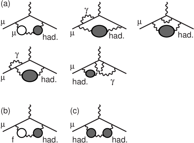
Figure 23: The three classes of diagrams (a,b,c) which contribute to $a_{\mu}^{\rm had,NLO}$. Class (a) contains the first five diagrams. In the class (b) diagram, $f=e$ or $\tau$, but not $\mu$. Mirror counterparts and diagrams with an interchange between the massless photon and the “massive photon” propagators should be understood.

The contributions from (2a), (2b), and (2c) can be written as

$$a_{\mu}^{\rm had,NLO(2a)} = \frac{\alpha}{4\pi^{4}}\int_{s_{\rm th}}^{\infty}{\rm d}s\,\sigma_{\rm had}^{0}(s)K^{(2a)}(s),$$ (177)

$$a_{\mu}^{\rm had,NLO(2b)} = \frac{\alpha}{4\pi^{4}}\int_{s_{\rm th}}^{\infty}{\rm d}s\,\sigma_{\rm had}^{0}(s)K^{(2b)}(s),$$ (178)

$$a_{\mu}^{\rm had,NLO(2c)} = \frac{1}{16\pi^{5}\alpha}\int_{s_{\rm th}}^{\infty}{\rm d}s\,\int_{s_{\rm th}}^{\infty}{\rm d}s^{\prime}\,\sigma_{\rm had}^{0}(s)\sigma_{\rm had}^{0}(s^{\prime})K^{(2c)}(s,s^{\prime}),$$ (179)

where the analytic expressions for $K^{(2a)},K^{(2b)}$ and $K^{(2c)}$ are given in Ref. [149]. We use the clustered data for the cross section for $e^{+}e^{-}\to{\rm hadrons}$, $\sigma_{\rm had}^{0}$ of (2), with the choice of inclusive data in the regime above 1.43 GeV to compute the contributions of the three different classes of NLO diagrams. We find

$$a_{\mu}^{\rm had,NLO(2a)} = (-20.73\pm 0.18_{\rm exp}\pm 0.07_{\rm rad})\times 10^{-10},$$ (180)

$$a_{\mu}^{\rm had,NLO(2b)} = (10.60\pm 0.09_{\rm exp}\pm 0.04_{\rm rad})\times 10^{-10},$$ (181)

$$a_{\mu}^{\rm had,NLO(2c)} = (0.34\pm 0.01_{\rm exp}\pm 0.00_{\rm rad})\times 10^{-10},$$ (182)

where we have assigned the uncertainty from the radiative correction similarly to the LO hadronic contribution. When summed,

$$a_{\mu}^{\rm had,NLO} = (-9.79\pm 0.09_{\rm exp}\pm 0.03_{\rm rad})\times 10^{-10},$$ (183)

which may be compared to the original calculation of Krause [149],

$$a_{\mu}^{\rm had,NLO}=(-21.1(0.5)+10.7(0.2)+0.27(0.01))\times 10^{-10}=-10.1(0.6)\times 10^{-10}.$$

In (183) we added the error linearly with an opposite relative sign since the errors in (2a) and (2b) are nearly 100% correlated in the opposite directions. Hence the total error is the difference of the two. In combining the errors we neglected the errors from (2c) since it is negligibly small compared to the other errors.

Note that the contribution of diagram (2c) does not agree with the result given by Krause, when account is taken of the small error on this contribution. We have therefore performed two checks of our numerical programme. First we replaced the two hadronic blobs of the diagram (2c) with two muon loops, since the contribution from such a diagram is known analytically [150] as a part of the QED contribution. It is

$$a_{\mu}({\rm two~{}muon~{}loops~{}along~{}one~{}photon~{}propagator})$$ (184)

$$= \left(\frac{\alpha}{\pi}\right)^{3}\left(-\frac{943}{324}-\frac{8}{45}\zeta(2)+\frac{8}{3}\zeta(3)\right)$$

$$= \left(\frac{\alpha}{\pi}\right)^{3}\times 0.002558\ldots$$ (185)

$$= 0.3206\ldots\times 10^{-10}.$$ (186)

Our programme reproduced $0.321\times 10^{-10}$, which agrees with (186) within an accuracy of $10^{-12}$, which is the accuracy of the calculation throughout this paper.

As a second check, we have taken $R(s)$ to be a step function. In the first line of Eq. (13) of the paper by Krause, the contribution from the diagram (2c) is written as a triple integral over $s$, $s^{\prime}$ and $x$, where $s$ and $s^{\prime}$ are ”mass-squared” of the hadronic blobs, and $x$ is a Feynman parameter. By explicitly integrating over $x$, Krause obtained the second line of Eq. (13), which is a double integral over $s$ and $s^{\prime}$. We are using this expression to integrate over the hadronic data. If $R(s)$ is a constant, we can explicitly integrate over $s$ and $s^{\prime}$, instead of $x$. Then we are left with one dimensional integral over $x$, which is much more tractable than the double integral over $s$ and $s^{\prime}$. We compared the result obtained from this integral over $x$ with the double integral over $s$ and $s^{\prime}$. Below are the numerical results.

When $R(s)$ is a constant (more rigorously, when $R(s)$ is a step function with $R(s)=1$ for $s>4m_{\pi}^{2}$, otherwise $R(s)=0$), the result from the double integral is

$$a_{\mu}=0.21\times 10^{-10},$$ (187)

(which has only two significant digits) and the result from the integral over $x$ is

$$a_{\mu}=0.2109\ldots\times 10^{-10}.$$ (188)

The agreement is very good. From the above two checks we believe our result for diagram (2c) is correct.

7.3 Hadronic contribution to $g-2$ of the muon

The hadronic contribution $a_{\mu}^{\rm had}$ has been divided into three pieces,

$$a_{\mu}^{\rm had}=a_{\mu}^{\rm had,LO}+a_{\mu}^{\rm had,NLO}+a_{\mu}^{\rm had,l\mbox{-}b\mbox{-}l}.$$ (189)

The lowest-order (vacuum polarisation) hadronic contribution, $a_{\mu}^{\rm had,LO}$, was calculated in Section 3. There we found

$$a_{\mu}^{\rm had,LO}=(692.4\pm 5.9_{\rm exp}\pm 2.4_{\rm rad})\times 10^{-10},$$ (190)

where we have used the QCD sum rule analysis to resolve the discrepancy in favour of the inclusive $e^{+}e^{-}\to{\rm hadrons}$ data in the region $1.4\;\raisebox{-3.01385pt}{$\stackrel{{\scriptstyle\textstyle<}}{{\sim}}$}\;\sqrt{s}\;\raisebox{-3.01385pt}{$\stackrel{{\scriptstyle\textstyle<}}{{\sim}}$}\;2$ GeV. The value of the next-to-leading order hadronic contribution, $a_{\mu}^{\rm had,NLO}$, was updated by the calculation described in the previous subsection. We obtained

$$a_{\mu}^{\rm had,NLO} = (-9.79\pm 0.09_{\rm exp}\pm 0.03_{\rm rad})\times 10^{-10}.$$ (191)

Finally, we must include the hadronic light-by-light scattering contribution $a_{\mu}^{\rm had,l\mbox{-}b\mbox{-}l}$. It has attracted much study. Recent re-evaluations can be found, for example, in Refs. [151]–[156]. Here we take the representative value

$$a_{\mu}^{\rm had,l\mbox{-}b\mbox{-}l}=(8.0\pm 4.0)\times 10^{-10},$$ (192)

as given in Ref. [157]. From Eqs. (176), (191) and (192), we can see that $a_{\mu}^{\rm had,LO}$ has the largest uncertainty, although the uncertainty in the light-by-light contribution $a_{\mu}^{\rm had,l\mbox{-}b\mbox{-}l}$ is also large.

When we combine all the three contributions to the hadronic contribution, we find

$$a_{\mu}^{\rm had}=(690.6\pm 7.4)\times 10^{-10}.$$ (193)

To calculate the number above, we first added the uncertainties associated with the LO and NLO diagrams linearly, and then added the uncertainty in the light-by-light contribution quadratically. We did so since the errors in the LO and the NLO contributions are nearly 100% correlated.

7.4 SM prediction of $g-2$ of the muon

The SM value of the anomalous magnetic moment of the muon, $a_{\mu}$, may be written as the sum of three terms,

$$a_{\mu}^{\rm SM}=a_{\mu}^{\rm QED}+a_{\mu}^{\rm EW}+a_{\mu}^{\rm had}.$$ (194)

The QED contribution, $a_{\mu}^{\rm QED}$, has been calculated up to and including estimates of the 5-loop contribution, see reviews  [144, 158, 159, 160],

$$a_{\mu}^{\rm QED}=116~{}584~{}703.5(2.8)\times 10^{-11}.$$ (195)

This value [160] includes the recent update from [144]. In comparison with the experimental error in Eq. (1), and the error of the hadronic contribution, the uncertainty in $a_{\mu}^{\rm QED}$ is much less important than the other sources of uncertainty. The electroweak contribution $a_{\mu}^{\rm EW}$ is calculated through second order to be [161]–[164]

$$a_{\mu}^{\rm EW}=154(2)\times 10^{-11}.$$ (196)

Here we quote the result of [164]. Although some discrepancies on conceptual questions remain, this result agrees numerically with the one of [163], and here again the error is negligibly small.

Summing up the SM contributions to $a_{\mu}^{\rm SM}$, as given in (193), (195) and (196), we conclude that

$$a_{\mu}^{\rm SM}=(11659176.3\pm 7.4)\times 10^{-10},$$ (197)

which is $26.7\times 10^{-10}$ ($2.4\sigma$) below the world average experimental measurement. If, on the other hand, we were to take, instead of (190), the value of $a_{\mu}^{\rm had,LO}$ obtained using the sum of the exclusive data in the interval $1.43<\sqrt{s}<2$ GeV, then we would find $a_{\mu}^{\rm SM}=(11659180.1\pm 7.4)\times 10^{-10}$, which is $22.9\times 10^{-10}$ ($2.1\sigma$) below $a_{\mu}^{\rm exp}$. The above values of $a_{\mu}^{SM}$ is compared with other determinations in Fig. 24.

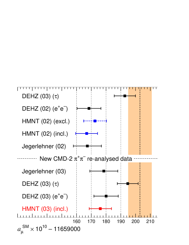
Figure 24: Recent evaluations of $a_{\mu}^{\rm SM}$ and the current world-average of the measured value (shown as a band). The band corresponds to a 1-$\sigma$ range. The final values, HMNT(03), are the predictions of this work, and include the recently re-analysed CMD-2 $\pi^{+}\pi^{-}$ data [10] in our analyses.

8 Determination of $\alpha_{\rm QED}(M_{Z}^{2})$

As mentioned in the Introduction, the value of the QED coupling at the $Z$ boson mass is the least well known of the three input parameters ($G_{\mu}$, $M_{Z}$ and $\alpha(M_{Z}^{2})$) which are the three most fundamental inputs of the standard electroweak model. Its uncertainty is therefore the limiting factor for precision electroweak physics. It is clearly important to determine $\alpha(M_{Z}^{2})$ as accurately as possible.

The value of $\alpha(M_{Z}^{2})$ is obtained from [104]

$$\alpha^{-1}\equiv\alpha(0)^{-1}=137.03599976(50)$$ (198)

using the relation

$$\alpha(s)^{-1}=\left(1-\Delta\alpha_{\rm lep}(s)-\Delta\alpha_{\rm had}^{(5)}(s)-\Delta\alpha^{\rm top}(s)\right)\alpha^{-1},$$ (199)

where the leptonic contribution to the running of $\alpha$ is known to three loops [169],

$$\Delta\alpha_{\rm lep}(M_{Z}^{2})=0.03149769.$$ (200)

The evaluation of the hadronic contribution, $\Delta\alpha_{\rm had}^{(5)}(M_{Z}^{2})$, is described below.

8.1 The hadronic contribution to the running of $\alpha$ up to $s=M_{Z}^{2}$

It is conventional to determine the contribution from 5 quark flavours, $\Delta\alpha_{\rm had}^{(5)}$, and to include the contribution of the sixth flavour [170],

$$\Delta\alpha^{\rm top}(M_{Z}^{2})=-0.000070(05),$$ (201)

at the end. The quark contribution cannot be calculated just from perturbative QCD because of low energy strong interaction effects. Rather we determined the contribution, $\Delta\alpha_{\rm had}^{(5)}(M_{Z}^{2})$, by evaluating the dispersion relation (46). The results were shown in Table 7. We found

$$\Delta\alpha_{\rm had}^{(5)}(M_{Z}^{2}) = 0.02755\pm 0.00019_{\rm exp}\pm 0.00013_{\rm rad,VP}\pm 0.000019_{\rm rad,FSR}$$ (202)

$$= 0.02755\pm 0.00019_{\rm exp}\pm 0.00013_{\rm rad}$$ (203)

$$= 0.02755\pm 0.00023,$$ (204)

if we use the inclusive measurements of $R(s)$ in the interval $1.43<\sqrt{s}<2\ {\rm GeV}$. The corresponding value of the QED coupling is given by

$$\alpha(M_{Z}^{2})^{-1}=128.954\pm 0.031.$$ (205)

If, on the other hand, we were to use the sum of the exclusive data for the various $e^{+}e^{-}\to{\rm hadron}$ channels, then the result would become $0.02769\pm 0.00018_{\rm exp}\pm 0.00013_{\rm rad}$ and $\alpha(M_{Z}^{2})^{-1}=128.935\pm 0.030$. Table 7 shows the contributions to $\Delta\alpha_{\rm had}^{(5)}(M_{Z}^{2})$ from the different energy intervals of the dispersion integral, (46), together with the sum. An alternative view may be obtained from the (lower) pie diagrams of Fig. 18. They display the fractions of the total contribution and error coming from various energy intervals in the dispersion integral. As anticipated, both Table 7 and the pie diagrams, show that the hadronic contributions to $\alpha(M_{Z}^{2})$ are more weighted to higher $s$ values in the dispersion integral for $\Delta\alpha_{\rm had}^{(5)}(M_{Z}^{2})$, than those in the integral for $a^{\rm had}_{\mu}$ needed to predict $g-2$ of the muon.

The above values of $\Delta\alpha_{\rm had}^{(5)}(M_{Z}^{2})$, and the corresponding values of $\alpha^{-1}$ at $s=M_{Z}^{2}$, are compared with other determinations in Fig. 25. The BES data [89] became available for the analyses from [133] onwards. In Table 10 we compare contributions to the dispersion relation (5) for $\Delta\alpha_{\rm had}^{(5)}(M_{Z}^{2})$ obtained in this work with those found by Burkhardt and Pietrzyk [100]. Since new $e^{+}e^{-}$ data became available for the former analysis, the comparison is only meaningful in the higher energy intervals. Nevertheless, although the agreement in the size of the contributions is good, we see that the latter analysis has considerably larger uncertainties in some energy intervals, which explains, in part, the difference in the size of the overall error shown in Fig. 25.

Table 9: The contributions of the individual $e^{+}e^{-}$ channels, up to $\sqrt{s}=1.8$ GeV, to dispersion relation (44) for $a_{\mu}^{\rm had,LO}\ (\times 10^{10})$ that were obtained in this analysis and in the DEHZ03 study [3]. The last column shows the difference. “Isospin” denotes channels for which no data exist, and for which isospin relations or bounds are used. We have divided the DEHZ $\omega$ contribution into the respective channels according to their branching fractions [104], with their sum normalized to unity.

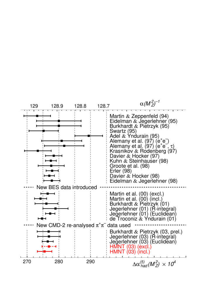
Figure 25: Recent determinations [99, 100, 108, 132, 133, 165, 167, 168, 170, 171, 172] of $\Delta\alpha_{\rm had}^{(5)}(M_{Z}^{2})$ (lower scale) with the corresponding value of $\alpha(M_{Z}^{2})^{-1}$ at the $Z$ boson mass shown on the upper scale. The last two entries, HMNT(03), are the values obtained in this work, and include the recent CMD-2 (re-analysed) data [10] in the evaluation.

energy range (GeV)	HMNT 03	BP 01
1.05–2.0	$16.34\pm 0.82$ (excl+incl)	$15.6\pm 2.3$ (excl)
	($5.56\pm 0.13$   (1.05–1.43 GeV, excl))
	($10.78\pm 0.81$   (1.43–2.0 GeV, incl))
2.0–5.0	$38.13\pm 1.10$ (incl)	$38.1\pm 2.2$ (incl)
5.0–7.0	$18.52\pm 0.64$ (incl)	$18.3\pm 1.1$ (incl)
7.0–12	$30.16\pm 0.61$ (incl+pQCD)	$30.4\pm 0.4$ (incl)
	( $25.32\pm 0.61$   (7.0–11 GeV, incl))
	( $4.84\pm 0.02$   (11–12 GeV, pQCD))
12–$\infty$	$120.48\pm 0.13$ (pQCD)	$120.3\pm 0.2$ (pQCD)

Table 10: Comparison of the contributions to $\Delta\alpha_{\rm had}(M_{Z}^{2})\times 10^{4}$ with the analysis of BP 01 [100].

8.2 Implications for the global fit to electroweak data

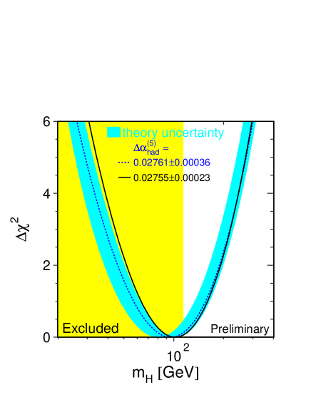
Figure 26: The $\chi^{2}$ profile versus the mass of a Standard Model Higgs boson obtained in a global analysis of electroweak data. The solid curve is obtained using the value we found in this work, and the dotted curve is obtained using the value in [100]. We thank Martin Grünewald for making this plot.

The value of the QED coupling on the Z pole is an important ingredient in the global fit of all the precise electroweak data. The continuous curve in Fig. 26 shows the $\chi^{2}$ profile as a function of $\ln m_{H}$ obtained in the global analysis if our value of $\Delta\alpha_{\rm had}$ is used. (whereas the dashed shows the profile that would result from the BP01 [100] determination of the QED coupling). The measured value of $m_{t}$ has been included in the analysis. When our new determination is taken, the fit predicts that a Standard Model Higgs has a mass

$$m_{H}=102\,^{\mbox{\normalsize+58}}_{-\mbox{\normalsize 38}}\ {\rm GeV}$$ (206)

or $m_{H}<221\ {\rm GeV}$ at the 95% confidence level.

9 Conclusions

The anomalous magnetic moment of the muon, $(g-2)/2$, and the QED coupling at the $Z$ boson mass, $\alpha(M_{Z}^{2})$, are two important quantities in particle physics. At present, the accuracy of the theoretical predictions is limited by the uncertainty of the hadronic vacuum polarization contributions. Here we use all the available data on $e^{+}e^{-}\to{\rm hadrons}$ to achieve the best presently possible data-driven determination of these contributions. In this way, we obtain a Standard Model prediction of the muon anomalous magnetic moment of

$$a_{\mu}^{\rm SM}=0.00116591763(74),$$ (207)

to be compared with the present experimental value of

$$a_{\mu}^{\rm exp}=0.0011659203(8),$$ (208)

which shows a $2.4\sigma$ difference. As this comparison of the measurement and prediction becomes more and more precise, we will obtain an increasingly powerful constraint on physics beyond the Standard Model.

We have also used our optimal compilation of the available $e^{+}e^{-}\to{\rm hadrons}$ data to predict

$$\alpha(M_{Z}^{2})^{-1}=128.954\pm 0.031.$$ (209)

The accuracy is now $24\times 10^{-5}$. This again is an important quantity. It is the most poorly-determined of the three parameters which specify the electroweak model. Although significantly improved from the error of Burkhardt and Pietrzyk’s preliminary result [172], it is still the least accurately determined of the three fundamental parameters of the electroweak theory; $\Delta G_{\mu}/G_{\mu}=1\times 10^{-5}$ and $\Delta M_{Z}/M_{Z}=2\times 10^{-5}$.

9.1 Future prospects for reducing the error on $g-2$

We have stressed that the comparison of the measurement and the Standard Model prediction of the muon anomalous magnetic moment, $a_{\mu}\equiv(g_{\mu}-2)/2$, is very important. It provides a valuable constraint on, or an indicator of, new physics beyond the Standard Model. From the above discussion, we see that the present uncertainties on the measurement and the prediction are 8 and 7 $\times 10^{-10}$ respectively. How realistic is it to improve the accuracy in the future? On the experimental side, the accuracy is dominated at present by the BNL measurement. We can expect a further improvement in the BNL measurement of $(g-2)$, since the collaboration are at present analysing 3.7 billion $\mu^{-}$ events which should give a total relative error of about 0.8 ppm. As a consequence, the $\pm 8\times 10^{-10}$ uncertainty in (208) should be improved to about $\pm 6\times 10^{-10}$. If the error on the theory prediction can be improved beyond this value then the case for another dedicated experiment with even more precision is considerably enhanced.

The error attributed to the theoretical prediction of $a_{\mu}$ is dominated by the uncertainties in the computation of the hadronic contribution, $a_{\mu}^{\rm had}$; in particular on the calculation of $a_{\mu}^{\rm had,LO}$ and $a_{\mu}^{\rm had,l\mbox{-}b\mbox{-}l}$, which at present have uncertainties of about 6 and 4 $\times 10^{-10}$ respectively. The latter error, on the light-by-light contribution, is generally believed to be able to be improved to 2 $\times 10^{-10}$ (25% error); and, optimistically, it is perhaps not hopeless to envisage an eventual accuracy of about 1 $\times 10^{-10}$ (10% error), but this would require a breakthrough in the understanding of this contribution. We are left to consider how much the error on $a_{\mu}^{\rm had,LO}$ could be improved. Already we are claiming a 1% accuracy. To reduce the error from the present 6 $\times 10^{-10}$ to 1 $\times 10^{-10}$ is not realistic. However we should note (see, for example, Ref. [173]) there will be progress from all experiments that are measuring $R$. Indeed, with the improvements, already in progress or planned, of the BES, CMD-3 + SND at VEPP-2000, BaBar, Belle, CLEO-C and KLOE experiments, we may anticipate an eventual accuracy of 0.5% in the crucial $\rho$ domain and 1-2% in the region above 1 GeV. It will be challenging, but not impossible. This statement also applies to improving the accuracy of the radiative corrections.

In this connection, note that the measurements of the radiative return experiments are just becoming available. From these experiments we may anticipate low energy data for a variety of $e^{+}e^{-}$ channels, produced via initial state radiation, at the $\phi$-factory DA$\Phi$NE [6, 9] and at the $B$-factories, BaBar and Belle, see, for example, [174]. For instance, by detecting the $\pi^{+}\pi^{-}\gamma$ channel, it may be possible to measure the vital $e^{+}e^{-}\to\pi^{+}\pi^{-}$ cross section in the threshold region. For the radiative return experiments there is no problem with statistics, and the accuracy is at present due to systematics, which come mainly from theory. These new experiments are motivating much theoretical work to improve their accuracy. Already, today, it is claimed to be 2% in the $\rho$ region.

In summary, we may hope for an improvement in accuracy down to about 3 $\times 10^{-10}$ in the theoretical prediction of $a_{\mu}$ in the foreseeable future, which in turn emphasizes the need for an experimental measurement with improved precision.

Note added in proof

The BNL muon $g-2$ collaboration have just published [178] the results of their analysis of the $\mu^{-}$ data which updates their experimental determination of $a_{\mu}$. As a result they now obtain a new world average

$$a_{\mu}^{\rm exp}=0.0011659208(6)\,.$$ (210)

Comparing this value with our SM prediction of Eq. (207) we find a $3.3\sigma$ discrepancy, as shown by the HMNT (03) (incl.) error bar in Fig. 27. That is the discrepancy is $\delta a_{\mu}=(31.7\pm 9.5)\times 10^{-10}$.

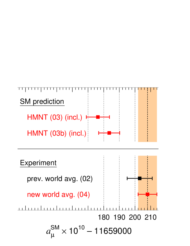
Figure 27: The new (world average) experimental value of the muon $(g_{\mu}-2)/2\equiv a_{\mu}$ given in Ref. [178], compared with the SM prediction as given in the text, HMNT (03), and with the value, HMNT (03b), which is obtained using the hadronic light-by-light contribution as recently calculated in Ref. [179] and the updated QED contribution given in Ref. [180].

Also, very recently, the hadronic light-by-light contribution has been recalculated, paying particular attention to the matching between the short- and long-distance behaviour [179]. The contribution is found to be $a_{\mu}^{\rm had,l\mbox{-}b\mbox{-}l}=(13.6\pm 2.5)\times 10^{-10}$. In addition Kinoshita and Nio have updated the calculation of the $\alpha^{4}$ QED contribution and find [180]

$$a_{\mu}^{\rm QED}=116584719.35(1.43)\times 10^{-11},$$ (211)

which should be compared with the value (195) we have used. If we use these new $a_{\mu}^{\rm had,l-b-l}$ and $a_{\mu}^{\rm QED}$ values, then our prediction is given by the HMNT (03b) (incl.) error bar in Fig. 27, and corresponds to

$$a_{\mu}^{\rm SM}=(11659183.53\pm 6.73)\times 10^{-10}$$ (212)

in the place of Eq. (207). If this prediction is compared with the new BNL result above, then there is a discrepancy of $2.7\sigma$, that is $\delta a_{\mu}=(24.5\pm 9.0)\times 10^{-10}$.

Appendix A: Threshold behaviour of $\pi^{0}\gamma$ and $\eta\gamma$ production

We take the Wess-Zumino-Witten (WZW) local interaction as

$${\cal L}_{WZW}=-\frac{\alpha}{8\pi f_{\pi}}c_{P}PF_{\mu\nu}\widetilde{F}^{\mu\nu},$$ (213)

where $f_{\pi}\simeq 93$ MeV, and $P$ denotes the electrically neutral members, $\pi^{0}$ or $\eta_{8}$, of the $SU(3)$ pseudoscalar octet. The $c_{P}$ coefficients are $c_{\pi^{0}}=1$ and $c_{\eta_{8}}=1/\sqrt{3}$. We may extend the multiplet to include the $SU(3)$ singlet, $\eta_{1}$, for which the coefficient is $c_{\eta_{1}}=2\sqrt{2}/\sqrt{3}$. As usual, $F_{\mu\nu}$ is the QED field strength tensor, and $\widetilde{F}_{\mu\nu}$ is its dual,

$$\widetilde{F}_{\mu\nu}\equiv\epsilon_{\mu\nu\rho\sigma}{F}^{\rho\sigma},$$ (214)

where $\epsilon_{\mu\nu\rho\sigma}$ is a totally antisymmetric tensor with $\epsilon_{0123}=1$.

A.1: $\pi^{0}\to 2\gamma$ decay and $e^{+}e^{-}\to\pi^{0}\gamma$

The WZW interaction, (213), is responsible for the $\pi^{0}\to 2\gamma$ decay. The lowest-order amplitude ${\cal M}$ is

$${\cal M}=\frac{\alpha}{\pi f_{\pi}}~{}\epsilon^{\mu\nu\lambda\sigma}~{}p_{1\mu}~{}p_{2\lambda}~{}\epsilon^{\ast}_{\nu}(p_{1})~{}\epsilon^{\ast}_{\sigma}(p_{2}),$$ (215)

which results in the partial decay width

$$\Gamma(\pi^{0}\to 2\gamma)=\frac{\alpha^{2}m_{\pi^{0}}^{3}}{64\pi^{3}f_{\pi}^{2}},$$ (216)

when summed over the polarization of the final state photons. If we take $f_{\pi}=(130\pm 5)/\sqrt{2}$ MeV and $m_{\pi^{0}}=134.9766\pm 0.0006$ MeV [104], then this gives

$$\Gamma(\pi^{0}\to 2\gamma)=7.81\pm 0.60~{}{\rm eV},$$ (217)

which is in good agreement with the experimental value [104],

$$\left.\Gamma(\pi^{0}\to 2\gamma)\right|_{\rm exp.}=7.7\pm 0.6~{}{\rm eV}.$$ (218)

The cross section of $e^{+}e^{-}\to\pi^{0}\gamma$ can be written in terms of the $\pi^{0}\to 2\gamma$ width as

$$\sigma(e^{+}e^{-}\to\pi^{0}\gamma)=\sigma_{\rm pt}(e^{+}e^{-}\to\pi^{0}\gamma)\equiv\frac{8\alpha\pi\Gamma(\pi^{0}\to 2\gamma)}{3m_{\pi}^{3}}\left(1-\frac{m_{\pi}^{2}}{s}\right)^{3}.$$ (219)

We can further improve the behaviour of the cross section by assuming vector meson dominance:

$$\sigma_{\rm VMD}(e^{+}e^{-}\to\pi^{0}\gamma)=\sigma_{\rm pt}(e^{+}e^{-}\to\pi^{0}\gamma)\left(\frac{m_{\omega}^{2}}{m_{\omega}^{2}-s}\right)^{2}.$$ (220)

We use the equation above in calculating the $\pi^{0}\gamma$ contribution from the threshold region in Section 3.1.

A.2: $\eta\to 2\gamma$ decay and $e^{+}e^{-}\to\eta\gamma$

If we neglect $\eta_{8}$-$\eta_{1}$ mixing and identify $\eta_{8}$ as $\eta$, then the $\eta\to 2\gamma$ decay is dictated by the WZW interaction,

$${\cal L}_{WZW}=-~{}\frac{\alpha}{8\sqrt{3}\pi f_{\pi}}~{}\eta_{8}~{}F_{\mu\nu}\widetilde{F}^{\mu\nu},$$ (221)

which contains an extra factor of $1/\sqrt{3}$ as compared with the $\pi^{0}\gamma\gamma$ coupling term. The calculation of the decay rate is exactly analogous to that of $\pi^{0}$ decay. The result is

$$\Gamma(\eta\to 2\gamma)=\frac{\alpha^{2}m_{\eta}^{3}}{192\pi^{3}f_{\pi}^{2}}~{}~{}~{}~{}~{}({\mbox{LO ChPT without $\eta_{1}$-$\eta_{8}$ mixing}}).$$ (222)

Taking $f_{\pi}=(130\pm 5)/\sqrt{2}$ MeV and $m_{\eta}=547.30\pm 0.12$ MeV [104], we obtain

$$\Gamma(\eta\to 2\gamma)=0.174\pm 0.013~{}{\rm keV}~{}~{}~{}~{}~{}({\mbox{LO ChPT without $\eta_{1}$-$\eta_{8}$ mixing}}),$$ (223)

which differs from the observed value [104] by about a factor of 3,

$$\left.\Gamma(\eta\to 2\gamma)\right|_{\rm exp.}=0.46\pm 0.04~{}{\rm keV}.$$ (224)

The agreement becomes better when we allow for the mixing between the $\eta$ and $\eta^{\prime}$ states. Following Ref. [175], we define the mixing angle $\theta_{P}$ by

$$\left(\begin{array}[]{c}\eta\\ \eta^{\prime}\end{array}\right)=\left(\begin{array}[]{rr}\cos\theta_{P}&-\sin\theta_{P}\\ \sin\theta_{P}&\cos\theta_{P}\end{array}\right)\left(\begin{array}[]{c}\eta_{8}\\ \eta_{1}\end{array}\right).$$ (231)

The Lagrangian now becomes

$${\cal L}=-\frac{\alpha}{8\pi f_{\pi}}\left(c_{\eta_{8}}\cos\theta_{P}-c_{\eta_{1}}\sin\theta_{P}\right)\eta F_{\mu\nu}\widetilde{F}^{\mu\nu}-\frac{\alpha}{8\pi f_{\pi}}\left(c_{\eta_{8}}\sin\theta_{P}+c_{\eta_{1}}\cos\theta_{P}\right)\eta^{\prime}F_{\mu\nu}\widetilde{F}^{\mu\nu}.$$ (232)

If we take $\theta_{P}\approx-20^{\circ}$ [175], then the coefficient of the $\eta F\widetilde{F}$ term is

$$c_{\eta_{8}}\cos\theta_{P}-c_{\eta_{1}}\sin\theta_{P}~{}=~{}1.91\times c_{\eta_{8}}~{}=~{}1.10,$$ (233)

and the predicted decay width is

$$\Gamma(\eta\to 2\gamma) = \frac{\alpha^{2}m_{\eta}^{3}}{64\pi^{3}f_{\pi}^{2}}(c_{\eta_{8}}\cos\theta_{P}-c_{\eta_{1}}\sin\theta_{P})^{2}$$ (234)

$$\simeq 0.63~{}{\rm keV}~{}~{}~{}~{}~{}({\mbox{LO ChPT with $\eta_{1}$-$\eta_{8}$ mixing}}).$$

We find the residual discrepancy with the observed rate is removed when we introduce the higher-order effect, $f_{1}\neq f_{8}\neq f_{\pi}$. In this case,

$${\cal L}=-\frac{\alpha}{8\pi}\left(\frac{c_{\eta_{8}}}{f_{8}}\cos\theta_{P}-\frac{c_{\eta_{1}}}{f_{1}}\sin\theta_{P}\right)\eta F_{\mu\nu}\widetilde{F}^{\mu\nu}-\frac{\alpha}{8\pi}\left(\frac{c_{\eta_{8}}}{f_{8}}\sin\theta_{P}+\frac{c_{\eta_{1}}}{f_{1}}\cos\theta_{P}\right)\eta^{\prime}F_{\mu\nu}\widetilde{F}^{\mu\nu}.$$ (235)

If we take $f_{8}\approx 1.3f_{\pi}$, $f_{1}\approx 1.1f_{\pi}$, as given by Eqs. (162) and (163) of Ref. [176], and $\theta_{P}\approx-20^{\circ}$, then the Lagrangian becomes

$${\cal L}\simeq-1.60\times\frac{\alpha}{8\pi f_{\pi}}c_{\eta_{8}}\eta F_{\mu\nu}\widetilde{F}^{\mu\nu},$$ (236)

and the predicted decay rate is

$$\Gamma(\eta\to 2\gamma) = \frac{\alpha^{2}m_{\eta}^{3}}{64\pi^{3}f_{\pi}^{2}}\left(\frac{f_{\pi}}{f_{8}}c_{\eta_{8}}\cos\theta_{P}-\frac{f_{\pi}}{f_{1}}c_{\eta_{1}}\sin\theta_{P}\right)^{2}$$ (237)

$$\simeq 0.45~{}{\rm keV}~{}~{}~{}~{}~{}({\mbox{NLO ChPT with $\eta_{1}$-$\eta_{8}$ mixing}}),$$

which is now in excellent agreement with the observed value, (224).

Similarly to the $e^{+}e^{-}\to\pi^{0}\gamma$ case, we can use the VMD approach to predict the cross section of $e^{+}e^{-}\to\eta\gamma$.

$$\sigma_{\rm VMD}(e^{+}e^{-}\to\eta\gamma)=\sigma_{\rm pt}(e^{+}e^{-}\to\eta\gamma)\left(\frac{m_{\omega}^{2}}{m_{\omega}^{2}-s}\right)^{2},$$ (238)

where

$$\sigma_{\rm pt}(e^{+}e^{-}\to\eta\gamma)\equiv\frac{\alpha^{3}}{24\pi^{2}}\left(\frac{c_{\eta_{8}}}{f_{8}}\cos\theta_{P}-\frac{c_{\eta_{1}}}{f_{1}}\sin\theta_{P}\right)^{2}\left(1-\frac{m_{\eta}^{2}}{s}\right)^{3}.$$ (239)

We take the parametrization (238) in calculating the $e^{+}e^{-}\to\eta\gamma$ cross section near the threshold region in Section 3.4.

Appendix B: Constraints on $V\to\sigma\gamma$ decay branching fractions

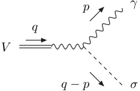
Figure 28: The $V\to\gamma\sigma$ decay in the VMD approach.

Here we calculate the $V\to\gamma\sigma$ decay of a vector meson using the Vector Meson Dominance (VMD) model. To calculate the amplitude, we have used the VMD Lagrangian [177]

$${\cal L}_{\rm VMD}=-\frac{1}{4}F_{\mu\nu}F^{\mu\nu}-\frac{1}{4}V_{\mu\nu}V^{\mu\nu}+\frac{1}{2}m_{V}^{2}V_{\mu}V^{\mu}-g_{V\pi\pi}V^{\mu}J_{\mu}-eJ_{\mu}A^{\mu}-\frac{e}{2g_{V}}F_{\mu\nu}V^{\mu\nu},$$ (240)

where $J_{\mu}$ is the electromagnetic current. $V_{\mu\nu}$ is defined by

$$V_{\mu\nu}\equiv\partial_{\mu}V_{\nu}-\partial_{\nu}V_{\mu}.$$ (241)

Here $V^{\mu}$ describes the neutral vector meson ($V=\rho,\omega,\phi,\cdots$). We take $e$ to be positive. The diagram which contributes to the decay is shown in Fig. 28. The amplitude ${\cal M}$ is given by

$$i{\cal M} = 4ig_{\sigma\gamma\gamma}((p\cdot q)g_{\alpha\beta}-p_{\alpha}q_{\beta})\left(-i\frac{eq^{2}}{g_{V}}\right)\frac{-i}{q^{2}}\epsilon_{\gamma}^{\beta\ast}(p)\epsilon_{V}^{\alpha}(q)$$ (242)

$$= -4ig_{\sigma\gamma\gamma}\frac{e}{g_{V}}((p\cdot q)g_{\alpha\beta}-p_{\alpha}q_{\beta})\epsilon_{\gamma}^{\beta\ast}(p)\epsilon_{V}^{\alpha}(q),$$

where $\epsilon_{V}$ and $\epsilon_{\gamma}$ are the polarization vectors of $V$ and the photon, respectively. We have assumed that the interaction between the $\sigma$ meson and photon is given by

$${\cal L}=g_{\sigma\gamma\gamma}\sigma F_{\mu\nu}F^{\mu\nu},$$ (243)

where $g_{\sigma\gamma\gamma}$ is a coupling constant. From the amplitude of (242) we can readily calculate the required partial decay width

$$\Gamma(V\to\gamma\sigma)=\frac{m_{V}^{3}}{6\pi}\left(\frac{eg_{\sigma\gamma\gamma}}{g_{V}}\right)^{2}\left(1-\frac{m_{\sigma}^{2}}{m_{V}^{2}}\right)^{3}.$$ (244)

If we use the parameters [104]

$$m_{\phi}=1019{\rm~{}MeV},~{}~{}~{}~{}~{}\Gamma_{\phi}=4.26{\rm~{}MeV},$$

$$g_{\phi}^{2}/\pi=14.4,~{}~{}~{}~{}~{}B(\phi\to\gamma\sigma)<0.002,$$ (245)

and assume $m_{\sigma}=600{\rm~{}MeV}$, then the coupling constant $g_{\sigma\gamma\gamma}$ is constrained to be

$$g_{\sigma\gamma\gamma}<5.2\times 10^{-4}({\rm MeV}^{-1}).$$ (246)

This bound gives constraints on $B(\omega\to\sigma\gamma)$ and $B(\phi(1.68)\to\sigma\gamma)$. From (244), the branching ratio $B(V\to\sigma\gamma)$ is

$$B(V\to\sigma\gamma)=\frac{2\alpha m_{V}^{3}}{3\Gamma_{V}}\left(1-\frac{m_{\sigma}^{2}}{m_{V}^{2}}\right)^{3}\frac{g_{\sigma\gamma\gamma}^{2}}{g_{V}^{2}}.$$ (247)

For the $\omega$ decay, we use the parameters

$$m_{\omega}=783{\rm~{}MeV},~{}~{}~{}~{}~{}\Gamma_{\omega}=8.44{\rm~{}MeV},~{}~{}~{}~{}~{}g_{\omega}^{2}/\pi=23.2,~{}~{}~{}~{}~{}m_{\sigma}=600{\rm~{}MeV},$$ (248)

to obtain the constraint

$$B(\omega\to\sigma\gamma)<7.2\times 10^{-5}.$$ (249)

Similarly, for the $\phi(1.68)\to\sigma\gamma$ decay, we have

$$B(\phi(1.68)\to\sigma\gamma)<3.5\times 10^{-5},$$ (250)

using the parameters

$$m_{\phi(1.68)}=1680{\rm~{}MeV},~{}~{}~{}~{}~{}\Gamma_{\phi(1.68)}=150{\rm~{}MeV},~{}~{}~{}~{}~{}g_{\phi(1.68)}^{2}/\pi=249,~{}~{}~{}~{}~{}m_{\sigma}=600{\rm~{}MeV}.$$ (251)

These constraints are used in Section 5.2.

References

- [1] G. W. Bennett et al., Muon Collaboration, Phys. Rev. Lett. 89 (2002) 101804, Erratum-ibid. 89 (2002) 129903.
- [2] M. Davier, S. Eidelman, A. Höcker and Z. Zhang, Eur. Phys. J. C27 (2003) 497.
- [3] M. Davier, S. Eidelman, A. Höcker and Z. Zhang, Eur. Phys. J. C31 (2003) 503, hep-ph/0308213.
- [4] S. Ghozzi and F. Jegerlehner, hep-ph/0310181.
-
[5]
H. Czyż, A. Grzelinska, J. H. Kühn and G. Rodrigo,
Eur. Phys. J. C27 (2003) 563;
hep-ph/0308312;
J. H. Kühn and G. Rodrigo, Eur. Phys. J. C25 (2002) 215;
G. Rodrigo, H. Czyż, J. H. Kühn and M. Szopa, Eur. Phys. J. C24 (2002) 71;
G. Rodrigo, Acta Phys. Polon. B32 (2001) 3833;
G. Rodrigo, A. Gehrmann-De Ridder, M. Guilleaume and J. H. Kühn, Eur. Phys. J. C22 (2001) 81. -
[6]
A. Aloisio et al., KLOE Collaboration,
hep-ex/0107023;
B. Valeriani et al., KLOE Collaboration, hep-ex/0205046;
S. Di Falco, KLOE Collaboration, Acta Phys. Polon. B34 (2003) 5207, hep-ex/0311006;
A. Aloisio et al., KLOE Collaboration, hep-ex/0307051. - [7] B. Aubert et al., BaBar Collaboration, Phys. Rev. D69 (2004) 011103, hep-ex/0310027.
- [8] Talk of M. Davier at the Workshop SIGHAD03, 8 – 10 October 2003, Pisa, Italy: “Results on from BaBar”, to appear in the proceedings.
-
[9]
A. Denig, KLOE Collaboration,
talk to 26th meeting of Scientific Committee, Frascati, May
2003;
A. Aloisio et al., KLOE Collaboration, hep-ex/0307051;
A. Denig, KLOE Collaboration, hep-ex/0311012. - [10] R. R. Akhmetshin et al., CMD-2 Collaboration, Phys. Lett. B578 (2004) 285, hep-ex/0308008.
- [11] R. R. Akhmetshin et al., CMD-2 Collaboration, Phys. Lett. B527 (2002) 161, hep-ex/0112031.
- [12] K. Hagiwara, A. D. Martin, D. Nomura and T. Teubner, Phys. Lett. B557 (2003) 69.
- [13] R. R. Akhmetshin et al., CMD-2 Collaboration, Phys. Lett. B476 (2000) 33, hep-ex/0002017.
- [14] R. R. Akhmetshin et al., CMD-2 Collaboration, Phys. Lett. B466 (1999) 385, hep-ex/9906032, Erratum-ibid. B508 (2001) 217.
- [15] M. R. Whalley, J. Phys. G29 (2003) A1.
- [16] I. B. Vasserman et al., OLYA Collaboration, Yad. Fiz. 30 (1979) 999, Sov. J. Nucl. Phys. 30 (1979) 519.
- [17] A. D. Bukin et al., OLYA Collaboration, Phys. Lett. B73 (1978) 226.
- [18] I. A. Koop, OLYA Collaboration, Preprint INP-79-67, Novosibirsk (1979).
- [19] I. B. Vasserman et al., OLYA Collaboration, Yad. Fiz. 33 (1981) 709, Sov. J. Nucl. Phys. 33 (1981) 368.
- [20] S. R. Amendolia et al., NA7 Collaboration, Phys. Lett. B138 (1984) 454.
- [21] L. M. Barkov et al., CMD, OLYA Collaboration, Nucl. Phys. B256 (1985) 365.
- [22] S. I. Dolinsky et al., CMD, ND, ARGUS Collaboration, Phys. Rept. 202 (1991) 99.
- [23] A. Quenzer et al., DM1 Collaboration, Phys. Lett. B76 (1978) 512.
- [24] D. Bisello et al., DM2 Collaboration, Phys. Lett. B220 (1989) 321.
- [25] D. Bollini et al., BCF Collaboration, Nuovo Cim. Lett. 14 (1975) 418.
- [26] M. Bernardini et al., BCF Collaboration, Phys. Lett. B46 (1973) 261.
- [27] B. Esposito et al., MEA Collaboration, Phys. Lett. B67 (1977) 239.
- [28] B. Esposito et al., MEA Collaboration, Lett. Nuovo Cim. 28 (1980) 337.
- [29] G. Cosme et al., ORSAY-ACO Collaboration, Preprint LAL-1287 (1976).
- [30] S. I. Eidelman, CMD-2 Collaboration, Nucl. Phys. Proc. Suppl. 98 (2001) 281.
- [31] M. N. Achasov et al., SND Collaboration, Phys. Lett. B559 (2003) 171, hep-ex/0302004.
- [32] M. N. Achasov et al., SND Collaboration, Eur. Phys. J. C12 (2000) 25.
- [33] M. N. Achasov et al., SND Collaboration, hep-ex/9710017, Preprint BINP-97-78, Novosibirsk (1997).
- [34] R. R. Akhmetshin et al., CMD-2 Collaboration, Phys. Lett. B364 (1995) 199.
- [35] R. R. Akhmetshin et al., CMD-2 Collaboration, Phys. Lett. B460 (1999) 242, hep-ex/9907003.
- [36] R. R. Akhmetshin et al., CMD-2 Collaboration, Phys. Lett. B509 (2001) 217, hep-ex/0103043.
- [37] A. Cordier et al., DM1 Collaboration, Nucl. Phys. B172 (1980) 13.
- [38] A. Antonelli et al., DM2 Collaboration, Z. Phys. C56 (1992) 15.
- [39] R. R. Akhmetshin et al., CMD-2 Collaboration, Phys. Lett. B434 (1998) 426.
- [40] M. N. Achasov et al., SND Collaboration, Phys. Rev. D66 (2002) 032001, hep-ex/0201040.
- [41] M. N. Achasov et al., SND Collaboration, Phys. Rev. D68 (2003) 052006, hep-ex/0305049.
- [42] L. M. Barkov et al., CMD Collaboration, Preprint BudkerINP 89-15 (in russian), Novosibirsk (1989).
- [43] P. M. Ivanov et al., OLYA Collaboration, Phys. Lett. B107 (1981) 297.
- [44] B. Delcourt et al., DM1 Collaboration, Phys. Lett. B99 (1981) 257.
- [45] D. Bisello et al., DM2 Collaboration, Z. Phys. C39 (1988) 13.
- [46] J. E. Augustin et al., DM2 Collaboration, Contributed to Int. Europhysics Conf. on High Energy Physics, Brighton, England, Jul 20-27, 1983.
- [47] M. N. Achasov et al., SND Collaboration, Phys. Rev. D63 (2001) 072002.
- [48] F. Mane et al., DM1 Collaboration, Phys. Lett. B99 (1981) 261.
- [49] R. R. Akhmetshin et al., CMD-2 Collaboration, Phys. Lett. B551 (2003) 27, hep-ex/0211004.
- [50] C. Paulot, M3N Collaboration, Thesis, LAL-79/14, Orsay (1979).
- [51] D. Bisello et al., DM2 Collaboration, Contributed paper to Int. Conf. on High Energy Physics, Singapore, Aug 2-8, 1990, see also LAL-90/35, Orsay (1990).
- [52] L. M. Kurdadze et al., OLYA Collaboration, JETP Lett. 43 (1986) 643.
- [53] R. R. Akhmetshin et al., CMD-2 Collaboration, Phys. Lett. B466 (1999) 392, hep-ex/9904024.
- [54] M. N. Achasov et al., SND Collaboration, J. Exp. Theor. Phys. 96 (2003) 789, Preprint BudkerINP2001-34 (in russian), Novosibirsk (2001).
- [55] G. Cosme et al., ORSAY-ACO Collaboration, Phys. Lett. B63 (1976) 349.
- [56] C. Bacci et al., Collaboration, Nucl. Phys. B184 (1981) 31.
- [57] B. Esposito et al., MEA Collaboration, Lett. Nuovo Cim. 31 (1981) 445.
- [58] R. R. Akhmetshin et al., CMD-2 Collaboration, Phys. Lett. B562 (2003) 173, hep-ex/0304009.
- [59] M. N. Achasov et al., SND Collaboration, Phys. Lett. B486 (2000) 29, hep-ex/0005032.
- [60] M. N. Achasov et al., SND Collaboration, Nucl. Phys. B569 (2000) 158, hep-ex/9907026.
- [61] S. I. Dolinsky et al., ND Collaboration, Phys. Lett. B174 (1986) 453.
- [62] L. M. Barkov et al., CMD Collaboration, Sov. J. Nucl. Phys. 47 (1988) 248.
- [63] A. Cordier et al., DM1 Collaboration, Phys. Lett. B109 (1982) 129.
- [64] A. Cordier et al., DM1-ACO Collaboration, Phys. Lett. B81 (1979) 389.
- [65] L. M. Kurdadze et al., OLYA Collaboration, JETP Lett. 47 (1988) 512.
- [66] C. Bacci et al., Collaboration, Phys. Lett. B95 (1980) 139.
- [67] R. R. Akhmetshin et al., CMD-2 Collaboration, Phys. Lett. B475 (2000) 190, hep-ex/9912020.
- [68] R. R. Akhmetshin et al., CMD-2 Collaboration, Phys. Lett. B491 (2000) 81, hep-ex/0008019.
- [69] R. R. Akhmetshin et al., CMD-2 Collaboration, Phys. Lett. B489 (2000) 125, hep-ex/0009013.
- [70] A. Cordier et al., DM1 Collaboration, Phys. Lett. B106 (1981) 155.
- [71] D. Bisello et al., DM1 Collaboration, Phys. Lett. B107 (1981) 145.
- [72] M. Schioppa, DM2 Collaboration, Thesis, Universita di Roma ‘La Sapienza’ (1986).
- [73] A. Antonelli et al., DM2 Collaboration, Phys. Lett. B212 (1988) 133.
- [74] D. Bisello et al., DM2 Collaboration, Nucl. Phys. Proc. Suppl. 21 (1991) 111, Preprint LAL-90-71, Orsay (1990).
- [75] D. Bisello et al., DM2 Collaboration, Z. Phys. C52 (1991) 227.
- [76] F. Mane et al., DM1 Collaboration, Phys. Lett. B112 (1982) 178.
- [77] F. Mané, DM1 Collaboration, Thesis, Université de Paris-Sud (1982), Preprint LAL 82/46.
- [78] A. Antonelli et al., FENICE Collaboration, Nucl. Phys. B517 (1998) 3.
- [79] A. Antonelli et al., FENICE Collaboration, Phys. Lett. B334 (1994) 431.
- [80] D. Bisello et al., DM2 Collaboration, Nucl. Phys. B224 (1983) 379.
- [81] D. Bisello et al., DM2 Collaboration, Z. Phys. C48 (1990) 23.
- [82] B. Delcourt et al., DM1 Collaboration, Phys. Lett. B86 (1979) 395.
- [83] A. Antonelli et al., FENICE Collaboration, Phys. Lett. B313 (1993) 283.
- [84] C. Bacci et al., Collaboration, Phys. Lett. B86 (1979) 234.
- [85] B. Esposito et al., MEA Collaboration, Lett. Nuovo Cim. 30 (1981) 65.
- [86] G. Cosme et al., M3N Collaboration, Nucl. Phys. B152 (1979) 215.
- [87] M. Ambrosio et al., BARYON-ANTIBARYON Collaboration, Phys. Lett. B91 (1980) 155.
- [88] J. Z. Bai et al., BES Collaboration, Phys. Rev. Lett. 84 (2000) 594, hep-ex/9908046.
- [89] J. Z. Bai et al., BES Collaboration, Phys. Rev. Lett. 88 (2002) 101802, hep-ex/0102003.
- [90] Z. Jakubowski et al., Crystal Ball Collaboration, Z. Phys. C40 (1988) 49.
- [91] A. Osterheld et al., Crystal Ball Collaboration, (1986), SLAC-PUB-4160.
- [92] C. Edwards et al., Crystal Ball Collaboration, (1990), SLAC-PUB-5160.
- [93] B. Niczyporuk et al., LENA Collaboration, Z. Phys. C15 (1982) 299.
- [94] A. E. Blinov et al., MD-1 Collaboration, Z. Phys. C70 (1996) 31.
- [95] H. Albrecht et al., DASP Collaboration, Phys. Lett. B116 (1982) 383.
- [96] R. Ammar et al., CLEO Collaboration, Phys. Rev. D57 (1998) 1350, hep-ex/9707018.
- [97] E. Rice et al., CUSB Collaboration, Phys. Rev. Lett. 48 (1982) 906.
- [98] P. Bock et al., DESY-Hamburg-Heidelberg-Munich Collaboration, Z. Phys. C6 (1980) 125.
- [99] M. L. Swartz, Phys. Rev. D53 (1996) 5268, hep-ph/9509248.
- [100] H. Burkhardt and B. Pietrzyk, Phys. Lett. B513 (2001) 46.
- [101] F. Jegerlehner, hep-ph/0308117.
- [102] A. Hoefer, J. Gluza and F. Jegerlehner, Eur. Phys. J. C24 (2002) 51, hep-ph/0107154.
- [103] J. Gluza, A. Hoefer, S. Jadach and F. Jegerlehner, Eur. Phys. J. C28 (2003) 261, hep-ph/0212386.
- [104] Review of Particle Physics: K. Hagiwara et al., Phys. Rev. D66 (2002) 010001.
- [105] Mini review of width, RPP, Phys. Rev. D66 (2002) 010001-743.
- [106] K. Hagiwara, A. D. Martin, D. Nomura and T. Teubner, in preparation.
- [107] See, for example, the review by K. G. Chetyrkin, J. H. Kühn and A. Kwiatkowski, Phys. Rept. 277 (1996) 189.
- [108] R. Alemany, M. Davier and A. Höcker, Eur. Phys. J. C2 (1998) 123.
- [109] G. D’Agostini, Nucl. Instrum. Meth. A346 (1994) 306.
- [110] T. Takeuchi, Prog. Theor. Phys. Suppl. 123 (1996) 247.
- [111] Talk of G. Fedotovitch at the Workshop SIGHAD03, 8 – 10 October 2003, Pisa, Italy: “Precise measurements of hadronic cross section at VEPP-2M”, to appear in the proceedings.
- [112] V. B. Berestetskii, O. N. Krokhin and A. K. Khelbnikov, JETP 3 (1956) 761.
- [113] N. N. Achasov and A. V. Kiselev, Phys. Rev. D65 (2002) 097302.
- [114] G. Colangelo, M. Finkemeier and R. Urech, Phys. Rev. D54 (1996) 4403.
- [115] S. R. Amendolia et al., NA7 Collaboration, Nucl. Phys. B277 (1986) 168.
- [116] E. A. Kuraev and Z. K. Silagadze, Phys. Atom. Nucl. 58 (1995) 1589 [Yad. Fiz. 58N9 (1995) 1687].
- [117] A. Ahmedov, G. V. Fedotovich, E. A. Kuraev and Z. K. Silagadze, JHEP 0209 (2002) 008.
- [118] A. Pais, Ann. Phys. 9 (1960) 548.
-
[119]
R. J. Sobie,
Z. Phys. C69 (1995) 99;
A. Rougé, Z. Phys. C70 (1996) 65. - [120] R. Barate et al., ALEPH Collaboration, Z. Phys. C76 (1997) 15.
- [121] A. Anastassov et al., CLEO Collaboration, Phys. Rev. Lett. 86 (2001) 4467.
- [122] R. R. Akhmetshin et al., CMD-2 Collaboration, hep-ex/0310012.
- [123] M. N. Achasov et al., SND Collaboration, Phys. Lett. B537 (2002) 201, hep-ex/0205068.
-
[124]
S. G. Gorishny, A. L. Kataev and S.A. Larin,
Phys. Lett. B259 (1991) 144;
L. R. Surguladze and M. A. Samuel, Phys. Rev. Lett. 66 (1991) 560;
Erratum-ibid. 66 (1991) 2416. - [125] K. G. Chetyrkin, A. H. Hoang, J. H. Kühn, M. Steinhauser and T. Teubner, Euro. Phys. J. C2 (1998) 137, hep-ph/9711327.
- [126] K. G. Chetyrkin, J. H. Kühn and M. Steinhauser, Nucl. Phys. B482 (1996) 213, hep-ph/9606230.
- [127] A. H. Hoang, M. Jeżabek, J. H. Kühn and T. Teubner, Phys. Lett. B338 (1994) 330, hep-ph/9407338.
- [128] R. Harlander and M. Steinhauser, Comput. Phys. Commun. 153 (2003) 244, hep-ph/0212294.
- [129] M. A. Shifman, A. I. Vainshtein and V. I. Zakharov, Nucl. Phys. B147 (1979) 385, 448, 519.
- [130] M. A. Shifman, Prog. Theor. Phys. Suppl. 131 (1998) 1.
- [131] K. G. Chetyrkin and J. H. Kühn, Phys. Lett. B248 (1990) 359.
- [132] M. Davier and A. Höcker, Phys. Lett. B419 (1998) 419.
-
[133]
A. D. Martin, J. Outhwaite and M. G. Ryskin,
Phys. Lett. B492 (2000) 69;
Eur. Phys. J. C19 (2001) 681. - [134] S. I. Eidelman, Nucl. Phys. Proc. Suppl. 98 (2001) 281.
- [135] R. Tenchini, private communication and discussions at the Workshop SIGHAD03, 8 – 10 October 2003, Pisa, Italy.
- [136] J. Gasser and U. G. Meissner, Nucl. Phys. B357 (1991) 90.
- [137] S. Narison, Phys. Lett. B568 (2003) 231.
- [138] T. Kinoshita, B. Nizic and Y. Okamoto, Phys. Rev. Lett. 52 (1984) 717; Phys. Rev. D31 (1985) 2108.
- [139] M. Hayakawa, T. Kinoshita and A. I. Sanda, Phys. Rev. Lett. 75 (1995) 790; Phys. Rev. D54 (1996) 3137.
- [140] J. Bijnens, E. Pallante and J. Prades, Nucl. Phys. B474 (1996) 379.
- [141] M. Hayakawa and T. Kinoshita, Phys. Rev. D57 (1998) 465; Erratum-ibid. D66 (2002) 019902 (E).
-
[142]
P. Mery, S. E. Moubarik, M. Perrottet and F. M. Renard,
Z. Phys. C46 (1990) 229;
A. I. Studenikin, Phys. Lett. B267 (1991) 117. - [143] R. D. Peccei, Phys. Lett. B136 (1984) 121.
- [144] T. Kinoshita and M. Nio, Phys. Rev. Lett. 90 (2003) 021803.
- [145] T. Kinoshita, private communication.
- [146] S. Laporta and E. Remiddi, Phys. Lett. B301 (1993) 440.
- [147] T. Kinoshita, J. Math. Phys. 3 (1962) 650.
- [148] T. D. Lee and M. Nauenberg, Phys. Rev. 133 (1964) B1549.
- [149] B. Krause, Phys. Lett. B390 (1997) 392.
- [150] J. A. Mignaco and E. Remiddi, Nuovo Cimento 60A (1969) 519.
- [151] M. Knecht and A. Nyffeler, Phys. Rev. D65 (2002) 073034.
- [152] M. Knecht, A. Nyffeler, M. Perrottet and E. de Rafael, Phys. Rev. Lett. 88 (2002) 071802.
- [153] M. Hayakawa and T. Kinoshita, hep-ph/0112102 and Erratum Phys. Rev. D66 (2002) 019902 (E).
- [154] J. Bijnens, E. Pallante and J. Prades, Nucl. Phys. B626 (2002) 410.
- [155] I. Blokland, A. Czarnecki and K. Melnikov, Phys. Rev. Lett. 88 (2002) 071803.
- [156] M. Ramsey-Musolf and M. B. Wise, Phys. Rev. Lett. 89 (2002) 041601.
- [157] A. Nyffeler, hep-ph/0203243.
- [158] V. W. Hughes and T. Kinoshita, Rev. Mod. Phys. 71 (1999) S133.
- [159] A. Czarnecki and W. J. Marciano, Nucl. Phys. Proc. Suppl. 76 (1999) 245.
- [160] A. Nyffeler, hep-ph/0305135.
- [161] A. Czarnecki, B. Krause and W. J. Marciano, Phys. Rev. D52 (1995) 2619; Phys. Rev. Lett. 76 (1996) 3267.
- [162] S. Peris, M. Perrottet and E. de Rafael, Phys. Lett. B355 (1995) 523.
- [163] M. Knecht, S. Peris, M. Perrottet and E. de Rafael, JHEP 0211 (2002) 003.
- [164] A. Czarnecki, W. J. Marciano and A. Vainshtein, Phys. Rev. D67 (2003) 073006.
-
[165]
S. Eidelman and F. Jegerlehner,
Z. Phys. C67 (1995) 585;
K. Adel and F. J. Ynduráin, hep-ph/9509378;
M. Davier and A. Höcker, Phys. Lett. B435 (1998) 427;
S. Eidelman and F. Jegerlehner, 1998 (cited in F. Jegerlehner, hep-ph/9901386). -
[166]
D. H. Brown and W. A. Worstell,
Phys. Rev. D54 (1996) 3237;
S. Narison, Phys. Lett. B513 (2001) 53; Erratum-ibid. B526 (2002) 414;
J. F. de Trocóniz and F. J. Ynduráin, Phys. Rev. D65 (2002) 093001;
G. Cvetič, T. Lee, and I. Schmidt, Phys. Lett. B520 (2001) 222. - [167] F. Jegerlehner, J. Phys. G29 (2003) 101, hep-ph/0104304.
- [168] F. Jegerlehner, hep-ph/0310234.
- [169] M. Steinhauser, Phys. Lett. B429 (1998) 158.
- [170] J. H. Kühn and M. Steinhauser, Phys. Lett. B437 (1998) 425, hep-ph/9802241.
-
[171]
A. D. Martin and D. Zeppenfeld,
Phys. Lett. B345 (1995) 558;
H. Burkhardt and B. Pietrzyk, Phys. Lett. B356 (1995) 398;
N. V. Krasnikov and R. Rodenberg, Nuovo Cim. A111 (1998) 217;
S. Groote et al., Phys. Lett. B440 (1998) 375;
J. Erler, Phys. Rev. D59 (1999) 054008, hep-ph/9803453;
J. F. de Trocóniz and F. J. Ynduráin, Phys. Rev. D65 (2002) 093002, hep-ph/0107318. - [172] H. Burkhardt and B. Pietrzyk, talk of B. Pietrzyk at the Workshop SIGHAD03, 8 – 10 October 2003, Pisa, Italy: “Fit of Standard Model, results on and influence on the Higgs mass”, to appear in the proceedings.
- [173] Talk of Z. Zhao at the Workshop SIGHAD03, 8 – 10 October 2003, Pisa, Italy: “Status and prospects or measurements”, to appear in the proceedings.
- [174] E. P. Solodov, hep-ex/0107027.
- [175] C. Amsler, Review on Quark Model, in Review of Particle Physics: K. Hagiwara et al., Phys. Rev. D66 (2002) 010001.
- [176] J. Bijnens, Int. J. Mod. Phys. A 8 (1993) 3045.
-
[177]
See, for example, J. J. Sakurai,
“Currents and Mesons”
(The University of Chicago Press, 1969);
H. B. O’Connell, B. C. Pearce, A. W. Thomas and A. G. Williams, Prog. Part. Nucl. Phys. 39 (1997) 201. - [178] G. W. Bennett et al., Muon Collaboration, hep-ex/0401008.
- [179] K. Melnikov and A. Vainshtein, hep-ph/0312226.
- [180] T. Kinoshita and M. Nio, hep-ph/0402206.