MCTP-03-55

UPR-1059

MADPH-03-1364

hep-ph/0312248

Relating Incomplete Data and Incomplete Theory

P. Binétruy¹, G. L. Kane², Brent D. Nelson³, Lian-Tao Wang⁴ and Ting T. Wang²

¹Laboratoire de Physique Théorique,

Université Paris-Sud, F-91405 Orsay, France

and APC, Université Paris 7, College de France, F-75231 Paris, France

²Michigan Center for Theoretical Physics, Randall Lab.,

University of Michigan, Ann Arbor, MI 48109

³Department of Physics, David Rittenhouse Lab.,

University of Pennsylvania, Philadelphia, PA 19104

⁴Department of Physics,

University of Wisconsin, Madison, WI 53706

Assuming string theorists will not soon provide a compelling case for the primary theory underlying particle physics, the field will proceed as it has historically: with data stimulating and testing ideas. Ideally the soft supersymmetry breaking Lagrangian will be measured and its patterns will point to the underlying theory. But there are two new problems. First a matter of principle: the theory may be simplest at distance scales and in numbers of dimensions where direct experiments are not possible. Second a practical problem: in the foreseeable future (with mainly hadron collider data) too few observables can be measured to lead to direct connections between experiment and theory. In this paper we discuss and study these issues and consider ways to circumvent the problems, studying models to test methods. We propose a semi-quantitative method for focusing and sharpening thinking when trying to relate incomplete data to incomplete theory, as will probably be necessary.

^∗This work was supported in part by grant number DE-FG02-95ER40893.

1 Introduction

We are living in an idea-rich era, when it comes to supersymmetric (SUSY) model-building. While the generic “problems” of SUSY models are often emphasized – the problem of dynamical SUSY breaking, the flavor problem, the problem of CP-violating phases, the $\mu$ problem, etc. – these problems are typically exhibited only for the sake of motivating a new solution. In fact most, if not all, of the generic problems of SUSY models have been “solved” several ways. Yet no “Supersymmetric Standard Model” exists. We believe the reason for the absence of such a model is not that none of the solutions mentioned above are satisfactory. Instead it is that most models of beyond the Standard Model physics based on supersymmetry only address one or two of these problems, with the remaining unaddressed problems leaving behind implicit large hierarchies and fine-tunings. As such these models cannot be considered realistic in the sense that they (of necessity) fail to explain a large segment of the world we observe experimentally.

This is a serious weakness given that even in the absence of direct evidence for superpartners we actually know a great deal about any possible supersymmetric model. The measured parameters of the Standard Model alone provide severe constraints on any putative supersymmetric Standard Model (SSM). Collider data, low-energy experiments and cosmological observations all provide further constraints. Yet the unrealistic nature of most SUSY models in the literature implies that only a small subset of this data is ever brought to bear on a given model. This deficiency will become even more obvious in the data-rich era of supersymmetry which we believe is at hand. One might contend that as soon as superpartners are directly observed models will rapidly improve. But consider (for example) a trilepton signal occurring at the LHC. Such an observation would be very exciting. It would give us some, but limited, information about chargino and neutralino masses – and even tell us something about the nature of dark matter. But it would not allow the measurement of SUSY Lagrangian parameters or $\tan\beta$. What it would tell us is for the most part already assumed in the model-building that has occurred thus far.

A supersymmetric Standard Model is likely to emerge only when we are able to take full advantage of the current and future data and understand how this data might connect to a fundamental theory such as string theory. This, in turn, is likely to require a change in strategy from all elements of our community. The standard approach of phenomenologists has been to assume that reconstructing a fundamental theory involves first measuring – often to a high degree of precision – the parameters of the soft supersymmetry-breaking Lagrangian which can then be connected to a supersymmetric Standard Model at a subsequent stage [1]. The standard approach of SUSY model-builders has been to assume that each of the issues that a SUSY standard model must address can be treated in isolation, with ingredients brought together and incorporated into a single model with ease at some later time. The standard approach of string theorists has been that any use of string constructions to guide this model building is premature, given our lack of a complete understanding of the space of all possible string theories. We believe that none of these assumptions is well justified and that enough information is available now, or may soon exist, to allow progress.

Perhaps past experience can provide some support for this view. When the Standard Model was formulated only a little was known and some only tentatively: the hadron spectrum, the existence of quarks and two neutrinos, currents were vector and axial vector, fermions were chiral, weak interactions were weak and early scaling in deep inelastic scattering. Theoretically the framework of gauge theories and the renormalizability of weak interactions were in place. Similar kinds of experimental information and theoretical structures are in place today. Some existing models are rather comprehensive and describe a lot of phenomena, yet they are not elevated to the position of supersymmetric standard models by the community. That may be because they involve fine-tunings and/or do not have a clear connection to an underlying theory such as string theory.

Thus we propose an improved way of thinking about how high energy models and experimental observations are to be connected in anticipation of the data-rich era expected to come. This approach is based on several principles. First, SUSY models must be made more realistic – efforts must be made to move beyond toy models to more holistic ones. This means models should begin to address all of the issues that a supersymmetric Standard Model might be expected to explain. Second, creative thinking is needed in identifying what we have called “inclusive signatures.” This means finding collider and non-collider observables which are both actual observables in existing and forthcoming experiments and which more directly probe the key features of supersymmetric Lagrangians. Third, we recommend finding ways in which observables from all arenas – low-energy, collider, cosmology, etc. – can be used in conjunction to get to the most likely paradigms as quickly as possible, and we propose a new method for doing so. This approach supplements and complements the more systematic bottom-up one of going from data to the Lagrangian at low energies to the high scale Lagrangian to the underlying (and presumably string) theory by helping to proceed with incomplete data.

In this paper we look at the state of the current approach by studying inclusive signatures and theoretical features of twelve benchmark points from twelve different models drawn from the current literature. The precise nature of these models is largely irrelevant to the new way of thinking we are proposing here, though we provide a very brief description of each model in Section 2; many readers can skip this section. We then use this survey as a backdrop in Section 3 for a discussion of how current and future data can provide considerable discriminatory power even before precision measurements of soft Lagrangian parameters are made. In Section 4 we introduce new ways of confronting the different theories with experimental data that seeks to maximize the power of incomplete data. Experimentalists may wish to read Sections 4.1, 4.3 and 4.4 first. We then make suggestions based on this new approach for model building and formal theory in Sections 5 and 6. In a concluding section we speculate on how a supersymmetric Standard Model will emerge and comment on how our suggestions might help bring that about.

2 A Sampling of Models

Our goal is to understand how the three elements we described above – formal theory, model building and phenomenology – work together to provide interpretations of observations and how this partnership can be made more efficient. The product of the combined efforts of these arenas, with input from experiments, should eventually be a supersymmetric Standard Model. Our own theoretical prejudice orients us towards models which are more likely to have a string-theoretic origin. However we here present twelve different models which span a wide spectrum of ideas. No effort was made to be absolutely comprehensive – nor do we make judgements here about the relative merits of any one model. Our one requirement is that the models admit some limit in which they can be treated as some form of MSSM model. All of the models we consider are designed to be consistent with the apparent unification of gauge couplings at some high scale. Thus we will not consider, for example, TeV-scale string models, models of (large) universal extra dimensions or little Higgs models.

The SUSY models described below primarily concern themselves with the parameters of the soft supersymmetry-breaking Lagrangian and hence the pattern of superpartner masses. We reiterate that the actual models chosen, as well as the specific point in the parameter space that we study, are largely irrelevant for the rest of the argument. The purpose of these summaries is to show the diversity of ideas current in the literature. Below we will briefly describe each model’s features before discussing the observational consequences and how one might distinguish between them in Section 3.

Model A: Generic mSUGRA.

The minimal supergravity (mSUGRA) model is defined by a universal soft supersymmetry-breaking gaugino mass $m_{1/2}$, a universal scalar mass $m_{0}$, a universal trilinear coupling $A_{0}$, as well as the electroweak parameters $\tan\beta$ and ${\rm sgn}(\mu)$. It is the simplest and most often studied model of supersymmetry breaking soft terms. We will pick a point in the low mass region of the allowed parameter space as a baseline for comparison with the other models to follow. The point we choose is Point B of Battaglia et al. [2], slightly adjusted to achieve a reasonable Higgs mass as in the first of the Snowmass Points and Slopes [3]: point SPS 1a. This point is given by $m_{0}=200~{}\mathrm{GeV}$, $m_{1/2}=250~{}\mathrm{GeV}$, $A_{0}=-800~{}\mathrm{GeV}$, $\tan\beta=10$ and positive $\mu$.

Model B: Hyperbolic/focus point mSUGRA.

There exists a locus of points in the mSUGRA parameter space for which large radiative corrections to the one-loop effective potential result in a small value of $\mu$ once the electroweak symmetry breaking (EWSB) constraint is imposed. For such “hyperbolic branch” points, the cancellations necessary to achieve a Z-boson mass of $M_{Z}=91~{}\mathrm{GeV}$ are greatly reduced [4]. Viewed in this way these points, which tend to involve large values of the (universal) scalar mass, may be considered “natural” in some sense. This view is strengthened by the observation that the running of the scalar soft mass $m_{H_{u}}^{2}$ exhibits a focus point behavior at low energies [5, 6, 7]. Thus the large scalar mass region of mSUGRA where the $\mu$ parameter is rapidly driven towards zero has come to be known as the “focus point” region – though the focus point behavior is operative throughout the mSUGRA parameter space.

We choose to define this region as the set of points for which $\mu\leq 250~{}\mathrm{GeV}$ with $m_{0}\geq 1~{}\mathrm{TeV}$. The precise location of this space for a given value of $m_{1/2}$ is theoretically uncertain and varies from one study to another depending on the analysis techniques employed. For our study we find an example with $\mu=210~{}\mathrm{GeV}$ for $m_{0}=2150~{}\mathrm{GeV}$ and $M_{1/2}=300~{}\mathrm{GeV}$ with vanishing A-term for $\tan\beta=10$. This point is similar to point SPS 2 [3] from the Snowmass Points and Slopes.

Model C: Minimal Gauge Mediation.

The gauge mediation model is characterized by a messenger sector which transmits the information of supersymmetry breaking from a hidden sector to the observable sector through gauge interactions [8]. In its minimal form this sector is assumed to comprise of N families of fields in a vector-like $\mathbf{5}+\mathbf{\overline{5}}$ representation of $SU(5)$ to preserve gauge coupling unification. The messengers are assumed to have universal (supersymmetric) mass $M_{\rm mess}$ and a mass splitting between scalars and fermions determined by the parameter $F$ such that observable sector soft masses are determined by the ratio $\Lambda=F/M_{\rm mess}$. These masses are presumed to be determined at the scale $\Lambda_{\mathsc{uv}}=M_{\rm mess}$. We will take as a representative point in the minimal gauge-mediated parameter space the case of the Snowmass point SPS 8 [3] with $\Lambda=100~{}\mathrm{TeV}$, $M_{\rm mess}=\Lambda_{\mathsc{uv}}=200~{}\mathrm{TeV}$, $N=1$ and $\tan\beta=15$.

Model D: Minimal Anomaly Mediation.

This is the original anomaly mediation model based on Kähler potentials of the sequestered sector form as suggested in [9, 10, 11]. The problem of tachyonic slepton masses arising first at two loop order is addressed through the addition of a universal contribution to scalar masses of undetermined origin. The phenomenology of this model was investigated in [12] and later incorporated into the Snowmass Points and Slopes as the point SPS 9 [3]. This is the point in the parameter space that we will investigate.

Model E: Anomaly Mediation with Ancillary U(1).

In this model the slepton problem of anomaly mediation is overcome by including the effects of an additional $U(1)$ D-term on scalar masses. This “ancillary” $U(1)$ is assumed to be anomaly-free using only the particle content of the MSSM. This restricts the possible $U(1)$ charge assignments which can be parameterized by two rational numbers [13]. Requiring that slepton mass-squareds be positive further restricts these choices. We will investigate the properties of an example in which the D-term contribution to scalar masses has a magnitude that is roughly three times the size of the typical scalar mass ($\eta=3$ in the language of [13]). We choose charge assignments such that $Q_{E}=1$ and $Q_{Q}=-1/10$ with a gravitino mass of $m_{3/2}=79~{}\mathrm{TeV}$.

Model F: Heterotic Strings with Kähler Stabilization.

The next two models involve weakly coupled heterotic string theory and are derived from the two most commonly employed methods for stabilizing the dilaton field – the field whose vacuum value determines the unified gauge coupling at the string scale. The first example is based on the “Kähler stabilization” method which assumes that nonperturbative corrections of string-theoretic origin arise for the dilaton action [14, 15, 16]. Then in the presence of one or more gaugino condensates in the hidden sector the dilaton can be stabilized at weak coupling ($g_{\mathsc{str}}^{2}=1/2$) with a vanishing vacuum energy, provided the parameters in the postulated nonperturbative correction are chosen properly [17, 18, 19].

Such models give rise to dilaton-dominated supersymmetry breaking, but the pattern of soft terms differs from the tree level examples often studied. In particular, gaugino masses and A-terms are suppressed relative to scalar masses by a loop factor with dilaton contributions and contributions from the conformal anomaly comparable in size. Examples of this scenario were presented in [20] and here we reproduce the case with condensing group beta-function coefficient $b_{+}=9/16\pi^{2}$ with a gravitino mass of $m_{3/2}=4300~{}\mathrm{GeV}$.

Model G: Heterotic Strings with Racetrack Stabilization.

At the other extreme from the previous model is the case where only the Kähler (compactification) moduli are involved in transmitting the supersymmetry breaking to the observable sector. This is a typical outcome in dilaton stabilization mechanisms that employ the tree level Kähler potential for the dilaton, as in the so-called “racetrack method” that uses multiple gaugino condensates to stabilize the dilaton [21, 22, 23]. Here the Kähler moduli tend to be stabilized slightly away from their self-dual points [24, 25].

When the observable sector matter fields all arise from the untwisted sector then the entire soft supersymmetry breaking Lagrangian arises only at the loop level. This was the case studied in [20], where we here use the case with gravitino mass of $m_{3/2}=20~{}\mathrm{TeV}$, Green-Schwarz counterterm coefficient $\delta_{\mathsc{gs}}=-9$ and $\left\langle{\rm Re}\;T\right\rangle=1.23$.

Model H: Heterotic Strings with Strong Coupling.

This model explores the strong-coupling limit of heterotic $E_{8}\times E_{8}$ string theory by studying the compactification of 11-dimensional M-theory on an $S_{1}/Z_{2}$ orbifold [26, 27, 28]. The low-energy effective Lagrangian for such a theory is characterized by deviations from the weakly coupled case in both the gauge kinetic function and the Kähler potential for the matter/moduli system [29]. These include the appearance of compactification moduli in the gauge kinetic function as well as the appearance of the dilaton in the kinetic function for the matter fields. These new contributions are proportional to a constant that is computable for a given compactification. The effect of these new terms is to allow the F-terms for the compactification moduli to play a role in determining soft gaugino masses while giving the dilaton F-term a role in determining the scalar masses.

Using the soft terms expressions as given in [30], we have chosen a point in parameter space where both the dilaton and the overall compactification modulus play equal roles in supersymmetry breaking. The fundamental scale is taken to be $\Lambda_{\mathsc{uv}}=\Lambda_{\mathsc{gut}}$ with $g_{\mathsc{str}}^{2}=1/2$, but with the size of the strong coupling correction such that this occurs for $\left\langle{\rm Re}\;S\right\rangle=1.25$ instead of the usual weakly coupled case of $\left\langle{\rm Re}\;S\right\rangle=2$.

Model I: Open Strings on Orientifolds with Common $D_{5}$ Branes.

In this example we consider a particular construction based on Type IIB string theory with toroidal orientifold compactification to four dimensions with $N=1$ supersymmetry [31]. For maximum simplicity we will place the entire Standard Model gauge group on a common set of $D_{5}$-branes whose world volumes are parallel to one another. Up to new contributions to the gauge kinetic functions from twisted moduli associated with the blowing-up modes of the orbifold singularities, this construction is very similar to the weakly coupled heterotic string at the tree level. Neglecting these additional twisted moduli contributions to gaugino masses is a good approximation in the limit where the single modulus that determines the gauge coupling is the sole participant in supersymmetry breaking [32]. In that limit the soft terms are given by $M_{1/2}=-A_{0}=\sqrt{3}m_{0}=\sqrt{3}m_{3/2}$, where $m_{3/2}$ is the gravitino mass.

This model has been studied at length in the literature [33, 34, 35] and it represents a special case of the mSUGRA paradigm. By couching it in the language of $D_{5}$-branes, however, one is at liberty to set the boundary condition (string) scale as a free parameter. The superpartner spectrum of this model in the case where this scale was taken to be $\Lambda_{\mathsc{uv}}=1\times 10^{11}~{}\mathrm{GeV}$ was studied in [36]. In order to achieve gauge coupling unification it is necessary to add additional exotic matter states to the theory at a low-energy scale. We follow a similar prescription to that of [36] and add two vector-like lepton doublets $(L,\overline{L})$ and three vector-like singlets $(E,\overline{E})$ at the TeV scale with hypercharge equal to their Standard Model equivalents. With this combination we find the unification scale to be $\Lambda_{\mathsc{uv}}=3\times 10^{11}~{}\mathrm{GeV}$.

Model J: Open Strings on Orientifolds with Intersecting $D_{5}$ Branes.

In our next open string example we will allow the gauge groups of the Standard Model to be localized on $D_{5}$-branes whose world-volumes are not parallel. We have in mind the case where the initial brane configuration is supersymmetric, with brane world-volumes intersecting at right angles. To obtain a specific model one must specify how fields and gauge groups are assigned to the various 5-branes. In [37] the following scenario was considered: assign the $SU(3)$ and $SU(2)$ gauge groups of the Standard Model to separate 5-branes. For ease of memory we will take $SU(3)$ to be on the $5_{3}$ brane and $SU(2)$ to be on the $5_{2}$ brane. This means, for example, that the world volume of the branes containing the $SU(3)$ gauge group have a world volume that spans the third complex plane. Quark doublets must then be the massless modes of strings that stretch between these branes. Hypercharge must be represented by some linear combination of the $U(1)$’s present on one or both branes. The decision of where to put the hypercharge $U(1)$ is crucial to the string assignment of the other Standard Model fields.

One possible configuration that allows for leading order Yukawa couplings for all third generation particles is to place the hypercharge factor solely on the $D_{5}$-branes containing the $SU(2)$ sector. In this set-up all quark superfields arise from the massless modes of stretched strings, while the lepton and Higgs superfields arise from massless modes of strings which start and end on the $5_{2}$ brane. To satisfy the string selection rules for the Yukawa interactions, the Higgs superfields will then need to have a Kähler potential with non-trivial dependence on the modulus associated with the first complex plane. We then choose the lepton singlet $E$ to have a Kähler metric which depends on the modulus of the second complex plane while that of the lepton doublet $L$ depends on the modulus of the first complex plane.

Assuming the perturbative (tree level) Kähler potential for all moduli fields, and all Kähler moduli $T_{1}$, $T_{2}$ and $T_{3}$ participating in supersymmetry breaking equally, we then have universal gaugino masses and trilinear couplings if the string scale and GUT scale coincide. The scalar masses would be given by $m_{H_{u}}^{2}=m_{H_{d}}^{2}=m_{E}^{2}=0$, $m_{Q}^{2}=m_{U}^{2}=m_{D}^{2}=(1/2)m_{3/2}^{2}$, $m_{L}^{2}=m_{3/2}^{2}$ and $M_{1/2}=-A_{0}=m_{3/2}$. At this point we may consider the non-parallel $D_{5}$-brane construction as nothing more than a motivation for studying a variant of the dilaton domination model with a particular pattern of non-universal scalar masses at $\Lambda_{\mathsc{uv}}=\Lambda_{\mathsc{gut}}$.

Model K: Minimal $SU(5)$ with Gaugino Mediation.

The minimal $SU(5)$ GUT-based model assumes that the $SU(5)$ gauge group is broken by the expectation value of a Higgs field in the 24 representation of $SU(5)$ at a scale $\Lambda_{\mathsc{gut}}\simeq 2\times 10^{16}~{}\mathrm{GeV}$ to the Standard Model. For gaugino mediation [38, 39] supersymmetry breaking is assumed to not occur at this scale but rather at a higher scale $M_{c}$ somewhere between the GUT scale and the Planck scale. As such, the soft supersymmetry breaking terms at $M_{c}$ obey GUT relations. The running of the soft Lagrangian between the two scales produces variations between the soft scalar masses associated with different representations under $SU(5)$, as well as generations within the same representation class.

The soft terms of this minimal model are assumed to be based on the notion that supersymmetry is broken in a hidden sector and is communicated to the observable sector through gauge multiplets which propagate in a higher-dimensional spacetime [40]. The construction of the model is such that only gaugino masses have non-zero soft masses at the leading order, with trilinear A-terms, bilinear B-terms and scalar masses zero at the same order. Collider signatures for the model described above were considered by Baer et al. [41]. They chose to leave the $\mu$ parameter and $B$ undetermined at the high-energy scale so that they can be fit by the EWSB conditions (allowing $\tan\beta$ to be a free parameter). We display results for their example point that has the unified parameters $m_{0}=205.2~{}\mathrm{GeV}$ and $M_{1/2}=400~{}\mathrm{GeV}$ with vanishing A-term and $\tan\beta=35$, but with positive $\mu$ term. These parameters are run in the GUT model from $M_{c}=1\times 10^{18}~{}\mathrm{GeV}$ to $1.52\times 10^{16}~{}\mathrm{GeV}$ and are run in the general MSSM model thereafter.

Model L: GUT-Inspired Minimal $SO(10)$.

The minimal $SO(10)$ GUT-based model of [42, 43] is based on the presumption that both gauge and Yukawa couplings unify at some scale $\Lambda_{\mathsc{gut}}$ into an $SO(10)$ framework. Assuming supersymmetry to be broken at the GUT scale, the model is defined by a universal gaugino mass $m_{1/2}$, a universal soft scalar mass $m_{16}^{2}$ for the matter fields in the 16 representation of SO(10), a universal soft scalar mass $m_{10}^{2}$ for the Higgs doublets in the 10 of SO(10), and a universal soft trilinear coupling $A_{0}$. To allow for proper electroweak symmetry breaking at the large values of $\tan\beta$ typically required for Yukawa unification, the Higgs masses are allowed to be split by some amount $\Delta m_{H}^{2}$, with the up-type Higgs mass $m_{H_{U}}^{2}$ decreased by this amount while the down-type Higgs mass $m_{H_{D}}^{2}$ is increased. We utilize a set of soft parameters determined, through a global $\chi^{2}$ analysis, to produce consistent EWSB and gauge/Yukawa unification at the scale $\Lambda_{\mathsc{gut}}\simeq 3\times 10^{16}~{}\mathrm{GeV}$ given known values of EW scale observables and fermion masses. The values are consistent with the results of Tobe and Wells [44].

We consider one of the representative points of [43] with $m_{16}=2000$, $m_{10}=2640$, $\Delta m_{H}^{2}=0.13m_{10}^{2}$, $A_{0}=-3420$, $M_{1/2}=350$ and $\mu=200$ in units of GeV. The value of $\tan\beta$ is 52.5. Note that in this model the boundary condition scale $\Lambda_{\mathsc{gut}}$ is part of the global fit, and is fixed to $3\times 10^{16}~{}\mathrm{GeV}$ for the specific point we consider. While this is a GUT-inspired model, no attempt is made to explain the Yukawa patterns of the first or second generation fermions, though first and second generation soft scalar masses are specified. Additionally, the specific model of [42, 43] did not specify any particular neutrino sector, though with additional assumptions one could be included quite easily.

3 Discriminating Between Models with “Observables”

We have taken the mass spectrum generated by the twelve model points of Section 2 and estimated the inclusive signatures of each case. By “inclusive signature” we are referring to a signature that indicates the existence of physics beyond the Standard Model, summed over all possible ways that such a signature can arise. An inclusive signature must be an actual physically observable quantity directly measured in experiments, such as the excess above some background of jet events with opposite-sign dileptons and missing transverse energy. It is important to understand that experiments only measure rates and kinematic distributions. Interpretation of results in terms of superpartner masses such as the gluino mass are necessarily model dependent and can be misleading. Essentially all soft Lagrangian parameters such as gaugino masses, the $\mu$ parameter and $\tan\beta$, etc. are unlikely to be directly measured.

The results of this estimation are included in the various rows of Table 1. This is, of course, just a partial list for purposes of illustration of the many measurable quantities that can now, or in the near future, help us to learn about the supersymmetric world. These quantities have been normalized in such a way that a “Y” indicates the presence of an observation that would clearly indicate new physics. More precise definitions of the signatures and the criteria used for assigning a “Y” value can be found in the Appendix. Let us note that the Y/N designation refers to the specific point in each model’s parameter space that was considered in Section 2. More generally, a model with “Y” in a given observable may be thought of as one which is likely to produce a signal throughout most of its parameter space. In collider situations with limited statistics (such as the Tevatron) or high backgrounds (such as the LHC) these inclusive signatures will be the initial signals observed. To go beyond them to soft Lagrangian parameters, or even to identify which superpartners are being produced and measure their masses, may require a long analysis and model-dependent assumptions. Thus learning what we can from the inclusive signatures alone could be essential.

The most important lesson to be learned from this table is that even with the difficulties outlined above, such as the failure of models to address vast amounts of data due to their incomplete nature, a handful of inclusive signatures may be sufficient to distinguish classes of these models! Strictly speaking, what can be distinguished are the specific points within these models’ parameter spaces that we chose to study. But to the extent that these points are truly representative then this is not merely an artifact of the points in parameter space that were chosen, but a property of the very real differences between the structure of these models. We expect that this is likely to be a robust feature of even wider arrays of models. Note that no specific soft Lagrangian parameters need to be measured – not even $\tan\beta$, whose value we have suppressed on purpose. The measurements envisioned in Table 1 are in no sense precision measurements but merely observations/non-observations. The data as seen by the experimentalist is similar to the columns we present here – a sequence of observations/non-observations with no “model name” to associate with the data or to assist in its interpretation. An important point is that experimenters can compare total event rates with those expected from the Standard Model and need not reduce samples with cuts.

Inclusive Signature

A

B

C

D

E

F

G

H

I

J

K

L

Collider

Large $E\kern-4.80005pt\hbox{/}\kern 0.40002pt_{T}$

Y

Y

Y

Y

Y

Y

Y

Y

Y

Y

Y

Y

Prompt $\gamma$

N

N

Y

N

N

N

N

N

N

N

N

N

Isolated $\pi^{\pm}$

N

N

N

N

N

N

Y

N

N

N

N

N

Trilepton

Y

Y

Y

N

N

Y

N

Y

Y

Y

Y

Y

SS dilepton

Y

Y

Y

N

N

Y

N

Y

Y

Y

Y

Y

OS dilepton

Y

N

Y

N

N

Y

N

Y

Y

Y

Y

N

$\tau$ rich

N

N

N

N

N

N

N

N

N

N

N

N

$b$ rich

N

N

N

N

N

N

N

N

N

N

N

N

Long-lived (N)LSP

Y

Y

Y

Y

Y

Y

Y

Y

Y

Y

Y

Y

Non-SM Flavor and CP

$g_{\mu}-2$

Y

N

Y

N

N

N

N

Y

N

N

Y

N

$B_{s}\to\mu^{+}\mu^{-}$

N

N

N

N

N

N

N

N

N

N

N

Y

$B\to X_{s}\gamma$

✓

✓

✓

✓

✓

✓

✓

✓

✓

✓

✓

✓

$A_{\mathsc{cp}}\left(B\to s\gamma\right)$

$\mathsc{sm}$

$\mathsc{sm}$

$\mathsc{sm}$

$\mathsc{sm}$

$\mathsc{sm}$

$\mathsc{sm}$

$\mathsc{sm}$

$\mathsc{sm}$

$\mathsc{sm}$

$\mathsc{sm}$

$\mathsc{sm}$

$\mathsc{sm}$

$A_{\mathsc{cp}}\left(B\to\phi K_{S}\right)$

$\mathsc{sm}$

$\mathsc{sm}$

$\mathsc{sm}$

$\mathsc{sm}$

$\mathsc{sm}$

$\mathsc{sm}$

$\mathsc{sm}$

$\mathsc{sm}$

$\mathsc{sm}$

$\mathsc{sm}$

$\mathsc{sm}$

$\mathsc{sm}$

$K-\overline{K}$ mixing

$\mathsc{sm}$

$\mathsc{sm}$

$\mathsc{sm}$

$\mathsc{sm}$

$\mathsc{sm}$

$\mathsc{sm}$

$\mathsc{sm}$

$\mathsc{sm}$

$\mathsc{sm}$

$\mathsc{sm}$

$\mathsc{sm}$

$\mathsc{sm}$

$\epsilon^{\prime}/\epsilon$

$\mathsc{sm}$

$\mathsc{sm}$

$\mathsc{sm}$

$\mathsc{sm}$

$\mathsc{sm}$

$\mathsc{sm}$

$\mathsc{sm}$

$\mathsc{sm}$

$\mathsc{sm}$

$\mathsc{sm}$

$\mathsc{sm}$

$\mathsc{sm}$

$\mu\to e\gamma$

$\mathsc{sm}$

$\mathsc{sm}$

$\mathsc{sm}$

$\mathsc{sm}$

$\mathsc{sm}$

$\mathsc{sm}$

$\mathsc{sm}$

$\mathsc{sm}$

$\mathsc{sm}$

$\mathsc{sm}$

$\mathsc{sm}$

$\mathsc{sm}$

$(2\beta)_{0\nu}$

eEDM, qEDM

$\mathsc{sm}$

$\mathsc{sm}$

$\mathsc{sm}$

$\mathsc{sm}$

$\mathsc{sm}$

$\mathsc{sm}$

$\mathsc{sm}$

$\mathsc{sm}$

$\mathsc{sm}$

$\mathsc{sm}$

$\mathsc{sm}$

$\mathsc{sm}$

Cosmology

Direct WIMP detection

N

N

N

N

N

N

N

N

N

N

N

${\rm Y}^{*}$

Space-based signals ($e^{+},\bar{p},\;\gamma$)

N

N

N

${\rm Y}^{*}$

${\rm Y}^{*}$

N

N

N

N

N

N

${\rm Y}^{*}$

Neutrinos from LSP annihilation

N

N

N

N

N

N

N

N

N

N

N

${\rm Y}^{*}$

Detectable axion

Baryon asymmetry

EWSB Sector

$M_{Z}$

EW precision data

✓

✓

✓

✓

✓

✓

✓

✓

✓

✓

✓

✓

Unification and Extended Sectors

Unified $\alpha_{\mathsc{gut}}(\Lambda_{\mathsc{uv}})$

✓

✓

✓

✓

✓

✓

✓

✓

✓

✓

✓

✓

$\alpha_{s}(M_{Z})=0.118$

TeV-scale exotic particles

N

N

N

N

N

N

N

N

Y

N

N

N

Proton decay

Table 1: Inclusive signature list for the twelve models. The general meaning of each of the signatures listed in the first column is given in the Appendix. Collider signatures are normalized to an LHC luminosity of $10{\rm fb}^{-1}$ for one year of running with a $5\sigma$ discovery threshold. We list a number of possible inclusive signatures to show what is possible, but at the present time there are few models that include all of the relevant physics. For observables that are basically ignored by the models we either leave the row blank, state that it gives the SM result in a trivial way, or use a ✓to indicate a non-trivial consistency check.

We break the listing into five categories: collider signatures, signatures of new physics in the flavor and CP violating arenas, cosmological signatures, the electroweak symmetry-breaking sector and signatures of models that go beyond the MSSM in content. Not surprisingly, all models are capable of making predictions in the collider arena and in most of the cosmological section since they all (at a minimum) predict the superpartner spectrum. But many rows are blank or give only the Standard Model result ($\mathsc{sm}$) in a trivial way. This is a reflection of the fact that none of these models address the strong CP problem (axions), have a neutrino sector ($(2\beta)_{0\nu}$), have phases (EDMs and CP asymmetries), or postulate specific Yukawa textures. All take R-parity conservation as a given fact and none address higher order operators, so none can make concrete predictions about proton decay (though some may allow it). All these models can say something about rare decays that could yield signals of new physics only in the limit where a signal can occur in the minimal flavor violation paradigm (such as the process $B_{s}\to\mu^{+}\mu^{-}$ or the muon anomalous magnetic moment), since all take the CKM matrix as inputs.

Still other observable quantities which have already been measured (such as the Z-boson mass and the strong coupling constant $\alpha_{s}(M_{Z})$) are taken as input quantities by all of these models. Thus the models are trivially consistent with these observations and do not explain these measured values. Indeed, this lack of explanation tends to reflect itself in large fine-tunings in, for example, the EWSB sector. To the extent that all of these models are designed to ensure gauge coupling unification, and assume all flavor structure is contained within the Standard Model CKM matrix, they can (in some limited sense) make predictions for the values of quantities such as the branching ratio ${\rm Br}(b\to s\gamma)$ and various electroweak precision variables. That they are consistent with the measured results (i.e. consistent with the hypothesis of no significant SUSY contributions) is merely a reflection of these starting assumptions. We have indicated this consistency with a check mark in Table 1.

Ultimately a complete model would provide meaningful predictions in the form of “Y” or “N” for each of these observables, or a “✓” that truly reflects a non-trivial consistency check on the theory. For example, most existing models would naively predict $M_{Z}$ to be an order of magnitude larger than it is if this mass were not already known. In each of the twelve models we consider this constraint is satisfied by taking $M_{Z}$ as an input rather than an output and assuming a fixed value of $\mu$ at the high scale to ensure this outcome. Without an explicit $\mu$-term generating mechanism this cannot be seen as a “prediction” for $M_{Z}$. As more observables are measured various rows in the table which currently display “Y/N” predictions become measured constraints. Models incapable of satisfying these constraints must, of course, then be modified or discarded.

Finally, there is yet another set of measured quantities that may be of use in determining the right supersymmetric Standard Model. We call these “derived observables” in that they are based on actually measured quantities, but the interpretation of that measurement can only be done in the context of a specific theory. For example, the WMAP experiment achieves a precise measurement of the non-baryonic cold dark matter density by fitting the observed CMB power spectrum to a number of input variables [45]. Thus, this quantity is measurable. If we wish to identify this observed matter component with a supersymmetric particle such as the lightest neutralino, then the necessary ingredients must be incorporated into a supersymmetric model: R-parity conservation, a relic production mechanism of thermal or non-thermal nature, and so on. Then this measurement becomes a constraint on the remaining parameter space (such as soft masses and $\tan\beta$) of this expanded model. But because these quantities either do not exist or are not calculable within the Standard Model, without a model it is not even clear what the WMAP observation is really measuring. Thus models that have all the requirements to make definite predictions about cold dark matter might be ruled out by this measurement – those that don’t are unaffected.

Or take the case of coupling unification – both gauge and Yukawa couplings. Strictly speaking this is a high-energy prediction of some models that is not directly testable. But once a model postulates the complete matter and gauge content of a theory, as well as a fundamental scale, then the observed gauge couplings are sufficient to “measure” the existence of a unified gauge coupling at some higher scale. We have included this “derived observable” in the Unification section of Table 1 since each of these models postulates the necessary assumptions to make such a derived quantity meaningful. So too the measured fermion masses, when coupled with an eventual measurement of $\tan\beta$ produces a “measurement” of Yukawa unification in the context of a complete model. Without such a complete model, these UV scale relations cease to have any meaning as observables.

Another example might be the degree of fine-tuning involved in satisfying a constraint. Once a quantity is measured, the tuning required to achieve this outcome is a legitimate observable to consider. While not directly measurable experimentally, once defined such tunings become a quantifiable derived observable that distinguishes between models. The discriminatory power of these derived observables is of help to the theorist in seeking ways to interpret the data. The mass of the Z-boson has been measured; hence the tuning on $M_{Z}$, however it is defined, becomes a distinguishing (theoretical) characteristic of models. Even the observed acceleration in the supernovas recession rate and the observable quantities associated with the cosmic microwave background radiation can become potential derived observables. We have not included such signatures in Table 1 but once a model identifies the inflaton with a field of the supersymmetric Standard Model, for example, then these parameters become fair constraints that such a model must satisfy.

4 Phenomenological Analysis

4.1 Discovery and Interpretation of Superpartners

While we may be lucky and find a superpartner signal at the Tevatron in spite of its poor performance, signals will surely appear at the LHC if low scale supersymmetry is present in nature. So let us present our analysis for LHC. Suppose supersymmetry-like excesses of events begin to be reported at LHC. What can be learned after the excitement of the raw discovery, given that there will be too few observables to deduce the underlying Lagrangian? To study this question we first simulate a possible signal, and then examine how far we can go in recovering the underlying physics.

The LHC experiments will measure production cross sections times branching ratios, and some kinematic distributions that will provide information about combinations of the eigenvalues of superpartner mass matrices. We assume $10{\rm fb}^{-1}$ integrated luminosity, i.e. one year at $10^{33}{\rm cm}^{-2}{\rm sec}^{-1}$, and consider the typical channels that will be studied. We further assume all channels involve missing transverse energy larger than $100~{}\mathrm{GeV}$ and at least two jets, each with transverse energy above $100~{}\mathrm{GeV}$. The excesses that are “discovered” differ in their leptonic properties (isolated energetic leptons). For the SM about 100,000 events are found with no leptons, 13,000 with one lepton, 7,000 with two opposite sign leptons, 20 with two same sign leptons, and 60 trileptons, all with large missing transverse energy. One model (Model F) gives respectively 31,700; 7,300; 2,000; 504; and 204 events for these channels in excess of the SM. Thus all channels show very statistically significant signals if we just use $\sqrt{N_{\mathsc{sm}}}$ as an approximate standard deviation. In addition, the peak of the so-called $m_{\rm eff}$ distribution (basically the sum of all transverse and missing energy) is at $838~{}\mathrm{GeV}$ for Model F. Some other kinematic distributions can be measured, such as the end points of the lepton $p_{T}$ distributions. There may also be information about the Higgs sector; for simplicity we won’t include that here. Table 2 shows the excesses for some of the other models in addition to Model F, as well as the Standard Model baseline.

Channel	SM	A	B	C	F	H	I	J	K	L
Jets ($\times 10^{3}$)	100.0	59.5	0.7	4.2	31.7	6.6	5.0	7.2	7.0	1.1
$1\ell$ ($\times 10^{3}$)	13.0	17.1	0.5	1.8	7.3	1.7	1.8	1.8	1.9	0.5
OS ($\times 10^{3}$)	7.0	5.7	0.2	1.1	2.0	0.6	0.8	0.8	0.6	0.2
SS	20	1332	99	277	504	160	252	155	197	90
$3\ell$	60	737	97	310	204	77	137	111	71	82
$m_{\rm eff}^{\rm peak}$ (GeV)	-	812	1140	1310	838	1210	1210	1340	1290	1210

Table 2: Number of events in excess of the Standard Model prediction for different signatures. For each channel the Standard Model baseline is given in the first column. Subsequent columns give the excess beyond this baseline for selected models from Section 2.

What can be learned from this information? From the event rates and distributions information can be obtained on the gluino mass and some squark, slepton, chargino and neutralino masses. The masses themselves cannot be measured accurately since there are not only significant experimental errors, but also considerable model dependence. Perhaps the lightest superpartner (LSP) mass can be measured at the 10-20% level. Remember that none of these masses correspond to Lagrangian parameters since they are radiatively corrected mass eigenstates, so we cannot determine the elements of the mass matrices (i.e. $\tan\beta$, the $\mu$ parameter magnitude and phase, the gaugino mass parameters $M_{1}$, $M_{2}$, $M_{3}$, etc). Even though we can’t determine these parameters, can we nevertheless extract information about the underlying theory?

Experimental analyses are (necessarily) done independently channel by channel. Measurement of the excess in any given channel will tell us little about the underlying theory since many sets of parameters in a given model, and many kinds of models, will give about the right number. What if we combine several channels? One can discuss this issue at several levels. First, suppose one knew or assumed a given basic model that contained several Lagrangian parameters. Can one then from a few actual experimental observables (that we call inclusive signatures) determine the basic parameters such as $\tan\beta$, $\mu$, gaugino masses, phases, etc.? Note that any such determination would necessarily have an associated model dependence because a priori   some other model might describe the data as well. We find that using the procedures we describe below leads to significant success here.

Second and more important, but more uncertain: could one, from a set of inclusive signatures, actually determine that some underlying theories (including the criteria which describe supersymmetry breaking itself) were significantly favored relative to others? In one sense this is not so hard, since some types of signatures are obviously special to some types of theories. For example, prompt photons only occur in gravity mediated theories if the LSP is Higgsino-like, and then only in certain types of events, while in gauge mediated theories every event has two prompt photons (unless the LSP is long-lived which can be tested for in other ways). But unless a lucky signature such as this occurs, it will be much more difficult to gain information about supersymmetry breaking or the high scale effective Lagrangian, let alone the corner of M-theory that is being seen, by normal methods. Consequently we have tried to develop an algorithmic approach that may lead to insights into the underlying theory even from inclusive signatures, and even when crucial quantities such as $\tan\beta$ have not yet been measured. We study these issues using models and simulated data in the following section.

To avoid misunderstanding we emphasize that the approach we describe is to help guide theorists toward what kind(s) of underlying theories and supersymmetry breaking to focus on. It is not meant to prove one theory is right, but to learn better what additional observables may provide particular sensitivity and what aspects of the theory need improved study and calculation. The method, a “global fit,” is in principle valid because all approaches, whatever the stringy connection and however supersymmetry is broken, connect to the observable world via the soft supersymmetry breaking Lagrangian.

4.2 Global theoretical fits

We study here an approach that we think may become a powerful technique to achieve the goals discussed above; that is, to relate incomplete data to the underlying theory. In essence, what we require is simultaneous consistency with several pieces of information (e.g. collider data, rare decays, relic neutralino interaction rates, and perhaps more as described below), and provide a quantitative measure to compare models and classes of models.

The idea of using likelihood techniques to identify favored areas of a model’s parameter space is certainly not new. The classic example is the global fit of the parameters of the Standard Model to electroweak precision measurements [47]. However, the notion that such an approach can be used to distinguish classes of models has not to our knowledge been pursued. Previous uses of this approach, which we call a $\chi_{T}^{2}$ (or theory $\chi^{2}$) analysis, tend to focus on only one model and often include “observations” that we have classified in Section 3 as derived observables such as Yukawa unification or the thermal relic density of neutralinos.

Rather than using a likelihood technique to find the most-favored point of a given parameter space, we propose using the $\chi_{T}^{2}$ technique to find the most-favored model in the space of theories. Let us see how such a procedure might work in the case of the twelve models of Section 2. Consider the minimal supergravity model with the following typical parameter set

$$\tan\beta=10\quad m_{1/2}=380\quad m_{0}=500\quad A_{0}=0\quad{\rm sgn}(\mu)>0.$$ (1)

The resulting low-energy soft Lagrangian is obtained through RG evolution of these parameters using SuSpect [48]. At the electroweak scale these values can be passed to PYTHIA [49] and an LHC collider simulation performed. We use the results of this simulation to calculate the number of events for the five inclusive signatures listed in Table 2 for a given luminosity.

Imagine the situation after the first year of data collection at the LHC. Experimental results for any excess above the Standard Model prediction, in each of the channels in Table 2, will be reported. Let us denote this excess by the vector

$$\vec{a}^{\rm exp}=\{a_{i}^{\rm exp}\}\quad i=1,2,\cdots,5,$$ (2)

and the expected Standard Model background by

$$\vec{a}^{\mathsc{sm}}=\{a_{i}^{\mathsc{sm}}\}\quad i=1,2,\cdots,5.$$ (3)

An estimation of the sizes of these background values for the LHC can be found in [63, 64].

Can we use the “experimental” result of (2) to reconstruct the mSUGRA point of (1)? We imagine dividing the parameter space of any model into a coarse grid with coordinate given by the parameter vector $\vec{x}$. For example, in the minimal supergravity model we would have

$$\vec{x}=\{m_{1/2},m_{0},\tan\beta,A_{0},{\rm sgn}(\mu)\},$$ (4)

while in the dilaton-dominated model $\vec{x}=\{m_{3/2},b_{+},\tan\beta\}$, and so forth. For each point labeled by $\vec{x}$ we will simulate some number of events (for illustrative purposes for this paper 30,000 events) within the framework of a particular model and compute the theoretical prediction $\vec{a}^{\rm th}=\{a_{i}^{\rm th}\}$. We then construct the quantity

$$\chi^{2}_{T}=\sum_{i=1}^{5}\frac{|a^{\rm th}_{i}(\vec{x})-a^{\rm exp}_{i}|^{2}}{\sigma_{i}^{2}}$$ (5)

where $\sigma_{i}^{2}$ is an experimental uncertainty of each value $a^{\rm exp}_{i}$ that we assign. For a Poisson distribution, $\sigma_{i}=\sqrt{a^{\rm exp}_{i}+a^{\mathsc{sm}}_{i}}$. Note that with this definition the contribution to $\chi^{2}_{T}$ from collider observables is proportional to the luminosity, so care is needed in interpreting $\chi^{2}_{T}$ and in choosing relative weights of collider and non-collider observables.

At this point questions could be raised about statistical measures, independent variables, etc. We think that is not a productive set of issues – at least not at this stage. In principle all of the models we study, to the extent that they are complete, specify a value for the 105 parameters of the MSSM. In most of the models we treat here the vast majority of these parameters are either zero or related in some simple manner. Nevertheless, one can imagine the space of these theories as being the space of the MSSM parameter set so that our theoretical measure is finding the best set of parameters for one model – the MSSM – but that best set may only be consistent with one class of MSSM paradigms represented by a particular type of theory. Theories where many of the parameters vanish or are strongly related tend to yield “$\mathsc{sm}$” in Table 1. But this merely indicates that some parameters in the theory (say, for example, the flavor structure of the soft supersymmetry-breaking trilinear couplings) play no role in determining the $\chi^{2}_{T}$ for that theory. In other cases where the theory makes a non-trivial prediction the quantities which receive “Y/N” predictions or “$\checkmark$” are included in the fit. In some sense the main difference, then, between this $\chi^{2}_{T}$ variable and the standard one used by experimentalists is that we seek to include only inclusive signatures. This measure can help us distinguish between models that appear, at first sight, to be extremely similar in nature. Two models that look similar in terms of there Y/N predictions in Table 1 may yield vastly different $\chi^{2}_{T}$ values in the fit, suggesting a differentiation not apparent before. This power is augmented when sensitivity, or fine-tuning measures are included in the analysis. The approach here should be treated as providing guidance and should not be used for conclusions such as “the heterotic string theory on an orbifold is $3.2\sigma$ better at fitting the data than the Type I theory…”.

	$m_{1/2}$ (GeV)
$m_{0}$ (GeV)	300	320	340	360	380	400	420	440	460	480
100	1097	471	175	60.6	16.9	3.6	2.5	6.4	12.7	19.4
200	792	363	159	63.3	20.1	6.3	7.2	15.1	23.5	34.7
300	528	244	94.9	36.6	15.5	10.9	14.2	23.8	33.5	43.6
400	445	166	53.7	16.3	5.7	8.2	14.7	27.8	37.1	46.0
500	427	207	37.2	9.3	1.7	7.6	16.5	28.7	39.7	49.4
600	248	668	70.6	20.6	5.5	10.0	20.8	31.0	42.2	51.7
700	197	255	136	35.6	16.2	16.2	21.9	33.7	44.9	54.9
800	178	214	57.0	51.2	18.7	23.3	28.3	36.9	45.5	55.2
900	133	34.4	27.8	27.3	29.1	29.8	34.8	41.4	49.5	56.2
1000	110	23.8	20.0	26.8	29.0	37.1	41.6	48.8	54.8	60.7

Table 3: Values of $\chi^{2}_{T}$ for the base mSUGRA model given by (1).

With these caveats in mind, we can now perform for each model a global inclusive fit to the theory by seeking the minimum $\chi^{2}_{T}$ by varying $\vec{x}$. Call this minimum $\chi^{2}_{T}$ as $\left(\chi^{2}_{T}\right)_{m}$. By comparing $\left(\chi^{2}_{T}\right)_{m}$ for different theories we can crudely identify the theory with the smallest value of $\left(\chi^{2}_{T}\right)_{m}$ as the most promising candidate. Furthermore, theories that yield $\left(\chi^{2}_{T}\right)_{m}\gg d$, where $d$ is the number of degrees of freedom (roughly the dimension of the vector $\vec{a}^{\rm exp}$ minus the dimension of $\vec{x}$) should be strongly disfavored. For the analysis we present below the five collider variables of Table 2 were included in all cases. In addition to the hypothesized LHC data we can also include other experimental results in the $\chi^{2}_{T}$ in a similar manner. In particular we also include experimental measurements of ${\rm Br}(b\to s\gamma)$ and $g_{\mu}-2$ with the following values: $a_{\mu}^{\mathsc{susy}}=(20\pm 20)\times 10^{-10}$ and ${\rm Br}(b\to s\gamma)=(3.25\pm 0.37)\times 10^{-4}$. Given that our purpose here is merely to illustrate the method, the actual values chosen are not important.

	$m_{1/2}$ (GeV)
$m_{0}$ (GeV)	300	320	340	360	380	400	420	440	460	480
100	$\mathsc{na}$	$\mathsc{na}$	$\mathsc{na}$	$\mathsc{na}$	$\mathsc{na}$	$\mathsc{na}$	$\mathsc{na}$	$\mathsc{na}$	$\mathsc{na}$	$\mathsc{na}$
200	616	275	119	59.2	$\mathsc{na}$	$\mathsc{na}$	$\mathsc{na}$	$\mathsc{na}$	$\mathsc{na}$	$\mathsc{na}$
300	617	271	115	51.4	16.2	4.8	7.3	15.1	26.5	35.9
400	442	192	59.5	21.1	8.2	8.5	16.7	23.5	32.9	39.1
500	383	135	35.6	7.4	2.7	7.8	17.3	27.5	37.7	48.1
600	203	139	26.6	5.7	2.4	10.1	21.7	32.6	42.2	50.7
700	141	80.6	32.0	7.9	7.9	13.4	24.6	34.1	45.6	55.6
800	136	95.5	34.8	22.3	34.7	20.3	28.3	37.4	45.8	55.8
900	90.5	76.1	20.7	24.7	29.7	30.1	35.5	42.9	51.2	58.2
1000	80.6	54.3	27.4	21.5	27.8	34.6	39.7	44.2	55.5	62.2

Table 4: Values of $\chi^{2}_{T}$ for the base mSUGRA model given by (1) but with $\tan\beta=40$. Entries marked $\mathsc{na}$ have a stau LSP.

Let us begin with the minimal supergravity model. The value of $\chi_{T}^{2}$ for each point in our coarse grid is given for $\mu>0$, $A_{0}=0$ and $\tan\beta=10$ in Table 3. The value of $\left(\chi^{2}_{T}\right)_{m}=1.7$ does indeed fall at the value input from (1). But in Table 3 we assumed the correct values of $\tan\beta$ and ${\rm sgn}(\mu)$. In Tables 4 and 5 we give the same region of the $(m_{1/2},m_{0})$ plane but change the value of $\tan\beta$ to $\tan\beta=40$ in Table 4 and the sign of $\mu$ in Table 5. In the former case the location of $\left(\chi^{2}_{T}\right)_{m}$ is displaced slightly while its value differs only slightly from the input case, so these inclusive signatures are not very sensitive to $\tan\beta$. In the latter case the location of $\left(\chi^{2}_{T}\right)_{m}$ is unchanged but the value has increased somewhat more. When both values are altered, as in Table 6, the location of the minimum shifts dramatically and the value of $\left(\chi^{2}_{T}\right)_{m}$ is much larger.

	$m_{1/2}$ (GeV)
$m_{0}$ (GeV)	300	320	340	360	380	400	420	440	460	480
100	689	326	151	89.8	64.1	40.8	31.6	28.6	28.8	30.7
200	793	380	174	73.5	29.6	16.1	13.1	21.3	30.9	38.6
300	512	232	102	47.9	24.3	17.5	23.3	30.5	37.6	45.3
400	408	163	64.5	22.9	11.3	13.9	21.4	31.1	42.4	49.0
500	457	144	46.1	14.9	7.0	11.2	21.7	32.7	42.2	52.0
600	233	261	80.2	29.4	9.7	14.1	23.1	33.8	45.1	53.5
700	188	176	144	47.8	22.3	19.0	25.4	35.8	45.3	55.6
800	146.8	51.4	63.7	63.7	68.3	24.9	30.6	38.2	46.3	56.0
900	106	28.2	44.8	35.9	35.0	38.7	36.5	42.8	49.8	57.8
1000	79.7	19.8	24.6	26.5	30.9	37.8	42.9	51.6	56.2	62.3

Table 5: Values of $\chi^{2}_{T}$ for the base mSUGRA model given by (1) but with $\tan\beta=10$ and $\mu<0$.

	$m_{1/2}$ (GeV)
$m_{0}$ (GeV)	300	320	340	360	380	400	420	440	460	480
100	$\mathsc{na}$	$\mathsc{na}$	$\mathsc{na}$	$\mathsc{na}$	$\mathsc{na}$	$\mathsc{na}$	$\mathsc{na}$	$\mathsc{na}$	$\mathsc{na}$	$\mathsc{na}$
200	1316	800	560	427	355	313	286	261	246	$\mathsc{na}$
300	1043	633	433	326	269	234	214	204	198	193
400	684	421	280	221	190	177	171	170	170	167
500	489	262	171	138	126	124	128	133	138	143
600	297	204	114	86.4	81.6	86.8	95.3	104	110	118
700	187	107	77.0	58.1	56.7	62.1	70.9	81.7	91.8	99.9
800	141	85.2	52.1	48.9	55.0	50.6	58.2	68.1	78.1	85.2
900	107	95.8	58.8	44.7	46.6	47.5	55.6	62.3	69.9	77.6
1000	81.1	74.0	31.2	37.2	41.2	47.9	52.6	57.4	68.5	74.5

Table 6: Values of $\chi^{2}_{T}$ for the base mSUGRA model given by (1) but with $\tan\beta=40$ and $\mu<0$. Entries marked $\mathsc{na}$ have a stau LSP.

Whether such differences are meaningful would require a more careful analysis. The Monte Carlo simulation involved in generating the quantities $\vec{a}^{\rm th}$ allows for possible statistical fluctuations. Since we only simulate a finite number of events there is always some uncertainty in the prediction. Therefore knowing whether the differences between Tables 3 and Tables 4 and 5 are significant would require generating an ensemble of such tables. Due to the computational intensity of such an undertaking we have not performed this analysis. When real data exists such an extended study would be worthwhile. Here we merely wish to examine the potential of the method.

An approximate measure of this uncertainty can be obtained by repeating the procedure several times. For example, consider the following mSUGRA point

$$\tan\beta=40\quad m_{1/2}=380\quad m_{0}=600\quad A_{0}=0\quad{\rm sgn}(\mu)>0.$$ (6)

Using PYTHIA we generated five tables such as those above using different random number seeds in each case and $N_{\rm event}=50,000$ events. Using the experimental “data” generated by the values in (1) we determined the value of $\left(\chi^{2}_{T}\right)_{m}$. For this exercise we include only the LHC collider signatures. In the limit as $N_{\rm event}\to\infty$ all five simulations should give identical answers. But the finite value of $N_{\rm event}$ allows for some variation in the outcomes. This variation is shown below in Table 7.

$\chi^{2}_{1}$	$\chi^{2}_{2}$	$\chi^{2}_{3}$	$\chi^{2}_{4}$	$\chi^{2}_{5}$	Mean
1.60	1.48	1.57	1.37	1.77	1.56

Table 7: Variation of values for $\left(\chi^{2}_{T}\right)_{m}$ for an ensemble of simulations.

The fluctuation on $\chi^{2}$ is approximately within $\pm 0.2$. It seems reasonable, therefore, to assume that the basic conclusion from Tables 3 through 6 is that while the sign of $\mu$ can be reliably determined from this small set of experimental observables the best fit $\chi^{2}_{T}$ is not sensitive enough to determine the value of $\tan\beta$.

So far we have been working only within a given theory so we have only been testing the rules of statistics which allow one to extract, from a set of data, the preferred values for the parameters of the theory. Nevertheless this exercise demonstrates the power of the technique since measuring $\tan\beta$ or $M_{1/2}$ by inverting formulas for cross-sections will not succeed in the short run, while this approach might – but the procedure is only valuable if we already know the “right” theory. What would be the result if we tried the same process with a different test theory?

We next wish to study whether the mSUGRA model itself can be selected from among the other models of Section 2. If so the method would become an exciting approach to how data can guide us to theory. Our set includes several models that are similar to minimal supergravity – both in terms of the input parameter set and the pattern of signatures given in Table 1. In particular let us consider models F and J. These are the weakly coupled heterotic model with Kähler stabilization and the open string model with $D_{5}$ branes, respectively.

Model F has three free parameters: the value of the beta-function coefficient for the condensing gauge group in the hidden sector, the value of the gravitino mass and $\tan\beta$. Model J is even more constrained, having only two free parameters apart from the sign of $\mu$: the value of $\tan\beta$ and the value of the gravitino mass. How well can these two models reproduce the experimental “data” generated from the mSUGRA point (1)? The best-fit point for the heterotic dilaton-dominated model with Kähler stabilization had the parameter values $\left\{m_{3/2}=2750~{}\mathrm{GeV}\;,\;b_{+}=24/16\pi^{2}\;,\;\tan\beta=5\right\}$ which corresponds to $\left(\chi^{2}_{T}\right)_{m}=2.8$. For the dilaton-dominated $D_{5}$-brane model the best fit point was given by $\left\{m_{3/2}=400~{}\mathrm{GeV}\;,\;\tan\beta=10\right\}$ which corresponds to $\left(\chi^{2}_{T}\right)_{m}=4.5$.

In Table 8 we collect these two best-fit points with the four preferred points from Tables 3 through 6. Note that the various models have different numbers of degrees of freedom. All utilize the five collider signatures plus the non-collider measurements of $g_{\mu}-2$ and ${\rm Br}(b\to s\gamma)$, giving a dimension of $\vec{a}^{\rm exp}$ of seven. The number of free parameters is the dimension of the vector $\vec{x}$, which is four for the mSUGRA models, three for Model F and two for Model J. We break down the overall contribution to the value of $\left(\chi^{2}_{T}\right)_{m}$ from each of the types of experimental data we consider, as well as giving the values of other kinematic data that could be used to discriminate between models. $M_{\rm eff}^{\rm peak}$ is the peak of the $M_{\rm eff}$ distribution where $M_{\rm eff}$ is defined as the sum of transverse energy of all jets plus $E\kern-6.00006pt\hbox{/}\kern 0.50003pt_{T}$. The quantity $m_{ll}^{\rm peak}$ is the peak of invariant mass distribution of the two leptons in the opposite sign dilepton events.

	mSUGRA $\tan\beta=10$		mSUGRA $\tan\beta=40$
	$\quad\mu>0\quad$	$\mu<0$	$\quad\mu>0\quad$	$\mu<0$	Model J	Model F
LHC	0.09	0.21	1.70	17.17	3.10	1.7
$a_{\mu}^{\mathsc{susy}}$	0.44	1.83	0.03	2.96	0.43	1.0
${\rm Br}(b\to s\gamma)$	1.16	4.96	0.66	11.09	1.00	0.1
Total $\left(\chi^{2}_{T}\right)_{m}$	1.69	7.00	2.39	31.22	4.54	2.8
d.o.f	3	3	3	3	4	5
$M_{\rm eff}^{\rm peak}$ (GeV)	1360	1260	1360	1438	1388	987
$m_{ll}^{\rm peak}$ (GeV)	92	92	92	92	92	58

Table 8: Breakdown of best-fit $\left(\chi^{2}_{T}\right)_{m}$ for different models. Each column represents the point in a model’s parameter space which minimizes $\chi^{2}_{T}$ in the corresponding model. The first four columns are mSUGRA models with different choices of $\tan\beta$ and sign of $\mu$. The fifth model is the $D_{5}$-brane model (Model J) and the last one is the heterotic dilaton-dominated model (Model F). We break down the total $\left(\chi^{2}_{T}\right)_{m}$ into contributions from the five collider signatures (“LHC”) as well as contributions from $a_{\mu}^{SUSY}$ and ${\rm Br}(b\to s\gamma)$. The kinematic variables $M_{\rm eff}^{\rm peak}$ and $m_{ll}^{\rm peak}$ are also given to show their utility in separating models.

By comparing the $\left(\chi^{2}_{T}\right)_{m}$ with the degrees of freedom for each model it is clear that an mSUGRA model with negative $\mu$ is disfavored. This is mainly due to the $b\to s\gamma$ constraint, and the discrepancy between the prediction of the theory and the experiment result gives a large $\chi^{2}_{T}$ contribution. The $D_{5}$-brane model is marginally compatible, with the primary contribution to $\chi^{2}_{T}$ coming from fitting the LHC data. The differences of $\left(\chi^{2}_{T}\right)_{m}$ between $\tan\beta=10$ and $\tan\beta=40$ (both with positive $\mu$) are not significant. This tells us that the observables we included in the $\chi^{2}_{T}$ fit are not sensitive to $\tan\beta$. Suppose at Tevatron or LHC there is a $B_{s}\to\mu^{+}\mu^{-}$ signal or sensitive limit, then we can include this observable into our $\chi^{2}_{T}$. Because of the large sensitivity of ${\rm Br}(B_{s}\to\mu^{+}\mu^{-})$ to $\tan\beta$ when the latter is large [50], such a signal can help us discriminate between models.

The dilaton-dominated heterotic model seems to be a good fit with the data, when one looks only at the $\chi^{2}_{T}$ variable. But notice that the kinematic observables for this model are very different from the other five cases. For the first four mSUGRA models the mass difference between $\tilde{N}_{2}$ and $\tilde{N}_{1}$ is larger than the $Z$ boson mass, so the peak of the $m_{ll}$ distribution, where $m_{ll}$ is the invariant mass of opposite sign dileptons, is around the $Z$ mass. For the dilaton-dominated model with Kähler stabilization this mass difference is smaller than $M_{Z}$ so the peak of $m_{ll}$ is significantly smaller than the others. If we take this kinematic observable into account, this dilaton-dominated SUSY breaking model should be disfavored.

Thus, in this simple example, the two mSUGRA models with positive $\mu$ give the best fit and the other models are disfavored. This example shows by using such a “theory global fit” approach, it is possible to gain information about underlying theories.

4.3 Identifying targeted inclusive signatures

If we focus our attention solely on the rows in Table 1 that we have been able to fill, we see that some model points are indeed distinguishable. But others are not and this differentiation is mild: many models differ from one another by a few inclusive signatures despite large differences in their underlying theory. If we were to subdivide the models even more this distinguishability between representative points of the models might be lost.

The origin of this mild differentiation can be traced to a number of factors. Perhaps principal among them is the sheer volume of existing data that any extension of the Standard Model must satisfy, not to mention constraints on the masses of new particles from direct search experiments or theoretical prejudices such as accounting for dark matter with relic neutralinos. Theories which a priori have quite different generic features tend to behave quite similarly once one restricts them to a set of parameters allowed by this data. Nevertheless, the phenomenological approach we advocate below could serve to estimate to what extent there is a similarity. For example, the minimal gaugino mediation model (Model K) has an identical set of inclusive signatures as that of the minimal gravity mediation model we considered (Model A). But this similarity ultimately stems from the fact that the GUT-nature of the gaugino mediation demands a universal gaugino mass and scalar mass at some point above the GUT scale (even though the actual values chosen for these parameters in Models A and K are quite different). If we were able to make real predictions for other observables we would undoubtedly find those which would be of most use in distinguishing between these two scenarios.

Another factor is the choice of inclusive signatures themselves. We have chosen the entries in the collider section of the table because these are the discovery modes that will be employed in SUSY searches at hadron colliders and thus they have been studied for some time. But while they may make excellent signatures for detecting beyond the Standard Model physics, they are often not signatures that are most directly tied to the key features of the underlying theories themselves. For example, the supersymmetric Higgsino mass parameter $\mu$ is a quantity whose value is unlikely to be measured directly until a linear collider with polarized lepton beams exists [51]. Even then extracting the value of this parameter will be a difficult challenge as there is no one experimental observable that is directly tied to its magnitude. Yet the value of the $\mu$-term is perhaps the most crucial parameter in the supersymmetric Lagrangian of the MSSM. Knowing it’s value, even approximately, might single out whole classes of theories by pointing to a superpotential vs. Kähler potential origin for this parameter and shed light on the soft Lagrangian through the fine-tuning of the Z-boson mass.

What is needed, then, is increased study towards identifying new signatures that more directly probe the Lagrangians of these models without necessarily reconstructing those Lagrangian parameters themselves. Call them “targeted inclusive signatures.” They will likely not be observables that are most efficient at discovering superpartners, but they may well prove extremely efficient at determining which subset of high energy theories is most likely to be correct. By constructing tables such as Table 1 using a variety of signatures the most powerful discriminants (i.e. the most targeted signatures) might become readily apparent.

It is important to keep in mind that these new signatures must be real observables. Many analyses on how underlying theories will be gleaned from data are based on measurements of what we will call “in-principle observables” (IPOs). These include soft Lagrangian parameters or ratios of parameters that are considered key indicators of some feature of a model. But such quantities may never be adequately measured – at least not to the precision that is often expected in order to distinguish between models. Even the soft gaugino mass parameters will require a suite of careful measurements to unambiguously reconstruct [52]. In order to get at the correct model as effectively as possible we must not mislead ourselves into treating these IPOs as actual observables, at least not for a long time. For the foreseeable future, except possibly for (approximately) the gluino mass, the only truly measurable quantities are the inclusive signatures. Nevertheless, the targeted inclusive signatures with the greatest discriminatory power are likely to be those which relate as closely as possible to the IPOs that are so often studied in the literature.

Some reflection upon the types of models considered in Section 2 – particularly those closely tied to string theories – suggests a few important distinguishing variables. To begin with, it is apparent that the pattern of gaugino masses is a distinctive signature of various transmission mechanisms of supersymmetry breaking. We have every reason to believe that more than one such mechanism (gauge mediation, anomaly mediation, moduli mediation, etc.) is likely to be present in nature. While one may be dominant over the others, there may be special circumstances such as a particular point in moduli space or a peculiar arrangement of the matter content of the theory such that two transmission mechanisms are competitive with one another. Furthermore, if gaugino masses are small at the tree level for one reason or another, then it is likely that the leading order gaugino masses will be nonuniversal. Thus a useful IPO would be the ratio

$${\cal O}_{1}\equiv\frac{M_{2}-M_{1}}{M_{3}}.$$ (7)

Another parameter of critical importance from a theoretical standpoint is the value of the fundamental mass scale of the theory. Here by fundamental scale we mean the scale at which the input parameters of the MSSM are set. In a string context we might think of this scale as the string scale. Though it does not have to be the case, it is typical to assume that this fundamental scale is to be identified with the scale of supersymmetry breaking in the observable sector. It is then often further assumed that this high-energy input scale is the GUT scale. Some indication of the magnitude of this fundamental scale can be obtained from the pattern of scalar masses at the low scale, in particular the difference between typical masses in the squark sector versus the slepton sector. Given that squark masses are generally strongly influenced over the course of their RG evolution by the gluino mass while slepton masses run very little, some measure of the size of the RG “desert” can be related to an IPO such as

$${\cal O}_{2}\equiv\frac{m_{\tilde{t_{1}}}^{2}-m_{\tilde{\tau_{1}}}^{2}}{M_{3}^{2}}.$$ (8)

Of course tree-level non-universalities in scalar masses at the input scale would obscure the impact of the RG running, but many models that predict such non-universality (such as gauge and anomaly mediated models) often involve characteristic splittings between squarks and sleptons that would make a quantity such as (8) a useful parameter.

Even the simple ratio of gaugino masses to scalar masses alone will be of critical importance in understanding the nature of supersymmetry breaking in a hidden sector and transmission to the observable sector. In minimal supergravity both scalar and gaugino masses are treated as free input parameters, but more sophisticated models often make predictions about the relative sizes of these masses since one may be generated at tree level while the other arises only at the loop level. Within the scalar sector itself the presence of large mass splittings in a sector other than the stop sector might reflect important information about scalar mass non-universality as well as the possible field dependence of trilinear coupling which appear in the off-diagonal entries of the scalar mass matrices. A potentially useful IPO might be the ratio

$${\cal O}_{3}\equiv\frac{m_{\tilde{{\tau}_{2}}}^{2}-m_{\tilde{\tau_{1}}}^{2}}{M_{1}^{2}}.$$ (9)

As important as these IPOs are for understanding the structure of the underlying supersymmetric theory, they are not in themselves directly measurable. Translating these quantities into inclusive signatures will necessarily obscure their relation to the fundamental Lagrangian somewhat. A good targeted inclusive signature would be one that is shown, through event simulation in real collider environments, to correlate well with the underlying IPO. Our efforts to identify such signatures based on the collider observables of Table 1 have thus far produced only limited success. The primary obstacle is the inclusive nature of the signature: when an observable arises through a combination of channels a strong correlation between that observable and the IPO may exist only for a particular hierarchy of masses or over a particular range of parameters.

Unfortunately, actually measuring any such observable may be very difficult. We have not found any such observables that are likely to be measurable before a linear collider exits, whenever that may be. Nevertheless, we are hopeful that further phenomenological study will produce targeted inclusive signatures with robust correlations to key soft Lagrangian combinations such as (7) - (9) and encourage others to suggest such observables. One avenue that may prove fruitful is the use of layered, or sequential, targeted signatures. That is, using the measured value of one inclusive signature as a key to indicate what subset of targeted observables will correlate well with the data.

We conclude this section by noting that the global inclusive fit to theory technique of the previous section may also lead in an indirect way to the targeted signatures we seek. The theories we study are defined by an input parameter vector $\vec{x}$ as in the case of (4) above. This defines a vector space that is the appropriate one for studying the underlying theory. But the inclusive signatures themselves depend on the low-scale values of the soft parameters. The mapping from the high to low scale is performed using the RGEs. Let us call the low-scale vector of soft parameters $\vec{y}=\vec{y}(\vec{x})$. This mapping is not one-to-one, but the elements of $\vec{y}$ are related in a known way.

The theory $\chi^{2}$ variable $\chi^{2}_{T}$ is a function of the original high-scale soft parameters only indirectly through the object $\vec{y}$. It is also a function of the observables we choose to include in the “experimental” result $\vec{a}^{\rm exp}$

$$\chi^{2}_{T}=f(\vec{y}(\vec{x});\,\vec{a}^{\rm exp}).$$ (10)

The targeted IPOs of Section 4.3, such as those suggested in equations 7, 8 and 9, represent a (non-linear) change of variables from the original vector $\vec{y}$ to a new vector $\vec{y}\,^{\prime}$. Similarly, targeted inclusive signatures would represent new observables $\vec{a}^{\rm exp}\,{}^{\prime}$ built from combinations of those in Table 1 (such as the ratios in Figure 1) – or as yet un-thought-of observables that can be measured. Finding combinations of $\vec{y}\,^{\prime}$ and $\vec{a}^{\rm exp}\,{}^{\prime}$ such that the functional form represented in (10) is as strong as possible means looking for combinations where the gradients along any particular component in $\vec{y}\,^{\prime}$ are as large as possible. This is essentially an algorithm for finding the optimal targeted observables and targeted IPOs, and may prove an invaluable tool in guiding us to measurements that will unravel the inter-related parameters of the supersymmetric Standard Model.

4.4 Comments for Experiments

As signals for physics beyond the Standard Model begin to emerge, particularly in collider data at the Tevatron or LHC, our approach has some impact on how data should be treated. Of course it will be important to learn which superpartners are being produced, to measure their masses, production cross sections and branching ratios, and to deduce Lagrangian parameters if possible. To do that, normally selections and cuts are performed on data to reduce backgrounds and isolate signals. At the Tevatron, with limited statistics, that procedure may reduce the signal so much that little can be learned. At LHC the large number of channels may make separation of states very difficult. Even if that were possible, at hadron colliders there are in general fewer observables than relevant Lagrangian parameters, so learning the essential Lagrangian quantities may not be possible except in special lucky situations.

Our approach has implications for these issues. We argue that the mere existence of certain classes of events – and the relative amounts of these different classes – point toward some classes of models and not others in useful ways. Thus experimenters should attempt fully or nearly inclusive measurements, without cuts that reduce statistics. It is, of course, essential to know the Standard Model predictions very well in order to recognize when they are exceeded.

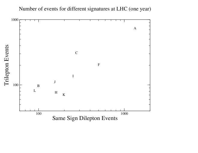
Figure 1: Distribution of Models. This figure illustrates how different models of high-energy physics tend naturally to produce different types of inclusive signatures. Combining such figures for several signatures could provide significant discriminatory power.

5 Comments for Model Building

It is both ironic and disappointing that the majority of the “predictions” being made by the bulk of SUSY models in the literature are in the one sector where we currently have precisely zero data: superpartner masses. Meanwhile we are blessed with large amounts of data from the other sectors displayed in Tables 1. The measurement of the Z-boson mass alone tells us a great deal about EWSB and how the $\mu$-term might be generated [53]. Electroweak precision measurements favor values of the oblique parameters that nearly (but perhaps not precisely) coincide with the Standard Model values, which tells us a great deal about any acceptable theory. Measurements at the Tevatron and the B-factories are providing important data on rare decays, mixing matrix entries and CP violation. The recent measurement of neutrino oscillations provides a whole sector awaiting a supersymmetric explanation. Cosmological observations have become sufficiently precise to rival terrestrial limits in some areas and are giving evidence for new classes of particles such as cold dark matter relics and quintessence fields. Indeed, a cosmological Standard Model is taking shape that cries out for (supersymmetric) explanations for dark matter, inflation and baryogenesis. Even null results in searches for certain theoretically well-motivated new fields as axions, fractionally-charged particles and $Z^{\prime}$-bosons provide important constraints on new models.

To be fair, there are a great many supersymmetry-based models in the literature that address each of these issues. But all too often this is done in isolation, with little or no regard to how the issues raised in say, rare decays may restrict the solutions at our disposal for understanding the origin of Yukawa textures or SUSY breaking in a hidden sector. It is our contention that the model builder must seek to treat the entire arena of inclusive signatures in as comprehensive a way as possible. We cannot completely neglect the theoretical framework in which these models arise – they cannot truly be reduced to the MSSM with an mSUGRA-like soft Lagrangian. The theory elements used to solve the various SUSY “problems” will manifest themselves in different ways depending on the construction. That is, there will always be some “back reaction” between, say, a $\mu$-term generating mechanism, or a flavor texture, on the low-energy predictions of the model. Thus dealing successfully with some problem is only an initial step towards solving the problem.

For example, models that utilize gauge mediation to communicate supersymmetry breaking to the observable sector have a particularly severe $\mu$ problem, or more specifically a $B\mu$ problem: it is difficult to engineer a $\mu$ and a $B\mu$ term that are both of electroweak scale size [8]. But like all such problems, many solutions have been proposed. If the $\mu$ term is generated by a higher-derivative operator as in the mechanism of [54] the problem can be solved, at the expense of adding two new singlets to the theory. This mechanism is economical and holistic in that the $\mu$ and $B\mu$ terms arise from the same mechanism as the other soft parameters in the theory. However, the Higgs soft scalar masses are also modified from the predictions of the minimal gauge mediated theory. This will, of course, affect the low energy phenomenology in a model-dependent way.

Another example involves combining a mechanism of generating Yukawa textures and supersymmetry breaking within an integrated string-based model [55]. If we treat Yukawa textures in isolation then there are a great many that have been designed to reproduce the correct fermion masses and mixings. In particular, it is possible to generate the appropriate textures using only a single Froggatt-Nielsen field $\varphi$ charged under a single Abelian $U(1)$ flavor group with a vacuum value $\left\langle\varphi\right\rangle\simeq\theta_{c}\simeq 0.2$ [56, 57, 58]. This single $U(1)$ mechanism works well when soft supersymmetry breaking can be ignored, as in the universal scalar mass paradigm. But since this $U(1)$ is necessarily broken by the vacuum value of $\varphi$, it is possible – even likely – that it will generate D-term contributions to the soft masses of the various Standard Model fields that are flavor dependent. Clearly, this changes the phenomenology of the model. In particular, it now becomes difficult to suppress the mixing in the $K-\bar{K}$ sector without resorting to two Abelian flavor factors. The flavor sector has affected the soft term phenomenology, which in turn has required a change in the flavor sector. Even if these D-term contributions could be eliminated, the model independent supergravity contribution to the trilinear A-terms proportional to $\left\langle\varphi\right\rangle m_{3/2}$ will provide non-universal contributions to the A-terms that are not proportional to the original Yukawa couplings [55]. The question of whether these contributions are phenomenologically dangerous now depends on the exact form of the superpotential, the soft Lagrangian and the size of the gravitino mass.

This is more than an academic exercise: most models that receive phenomenological study are those that are promoted on the basis of their perceived predictivity. That is to say, they are promoted on the basis of their apparent simplicity and the small number of free input parameters that they seem to have. But this is deceptive, as the examples above suggest. The question of how well these simple “paradigm models” approximate the realistic models we actually need to construct is an open question.

What is more, the way that experimental measurements are used to constrain models depends very much on the properties of a complete model. For example, if we choose to neglect the flavor sector of a model by tacitly assuming that degeneracy or alignment is at play, then we may use the minimal flavor violation model to calculate the implication of the CLEO and BELLE measurements of ${\rm Br}(B\to s\gamma)$ on the particle masses and the sign of the $\mu$ parameter of a given model. But when there are new sources of flavor violation in the soft Lagrangian, many other contributions must be included in the calculation which are not suppressed by CKM matrix elements [59]. It is even possible for this new contribution to be the dominant one, thus changing the interpretation of the experimental result [60]. A completely different set of constraints on the superpartner spectrum, and no effective constraint on the sign of $\mu$, is obtained. So without a complete model this important clue to the supersymmetric world cannot be properly utilized. A similar thing occurs in the neutralino cold dark matter scenario, where the interaction cross section of relic neutralinos with protons (as well as the relic density itself), depends crucially on the phases in the neutralino mass matrix [61]. How are we to properly interpret the implication of a dark matter detection signal – or apply the WMAP constraint on non-baryonic dark matter – without a theory that addresses the origin of $\mu$ and its relative phase with respect to gaugino masses?

The answer is, of course, quite familiar. We make assumptions that are simplifying in order to separate confounding issues and make progress. If these assumptions were justified then they might be put to the test at a later time with a different set of experiments – if the assumptions are very wrong this analysis is irrelevant. But without examples of complete models it is unclear what these cross-checking experiments might be. We suggest that in constructing models that are capable of filling in all the entries in tables such as Table 1 these relations will become much more obvious.

What might a complete model look like? The promise of supersymmetry is the opportunity to make meaningful statements about mass scales in the effective field theory below the string scale by protecting these scales from quadratic divergences. Thus a supersymmetric Standard Model should explain the dynamical origin of the mass scales relevant to observations: the supersymmetry breaking scale in the hidden sector, the scale of transmission of that breaking to the observable sector, the value of the $\mu$ parameter, the size of the Higgs vev, the axion decay constant, Majorana neutrino masses, the scale at which flavor symmetries are broken, etc. While conceptually distinct from issues of supersymmetry breaking and mass scales, a supersymmetric Standard model – to the extent that it is a deeper model than the non-supersymmetric Standard Model – should also identify the symmetries (if any) operative in the dimensionless parameters of the effective theory below the string scale. The origin of these parameters and the symmetries themselves are presumed to be in the domain of a future stringy Standard Model. Finally, the SSM we seek will be consistent with the constraints of Table 1 but will also provide an explanation for why this consistency is an inherent feature of the model itself by deriving this fact from deeper physics principles.

For example, we might ask what it might require to make mSUGRA a complete model. In truth it is already complete in some very limited sense: namely that the assumptions made in defining the mSUGRA paradigm are technically sufficient to fill in all of the entries of Table 1, though some in a very trivial way. Let us call this “minimal completeness:” mSUGRA is complete, but not truly a model because it does not contain an explanation for its various assumptions. In mSUGRA this comes about by postulating some hidden sector superfields which develop vacuum values for their auxiliary field components in a universal way. Yukawa matrices and the $\mu$ parameter are taken as (non-field-dependent) fixed parameters. The neutrino sector and cosmological issues are ignored. While this set of assumptions is technically sufficient to fill most of the entries in Table 1, it clearly provides no explanation of deeper physics principles and can only be thought of as a framework deserving of its title as “minimal.”

To make mSUGRA complete in the sense we use the term would require adding several elements to this minimal framework. The origin of these auxiliary field vacuum values would need to be explained and the vanishing vacuum energy outcome demonstrated through the construction of a concrete dynamical symmetry breaking mechanism. The reality of the soft terms should be traced to some symmetry or some mechanism for predicting the imaginary parts of the relevant vacuum expectation values. The $\mu$-term would be generated dynamically, either through some sort of Giudice-Masiero mechanism or superpotential vev so that its value could no longer be taken as an input but instead be tied to other parameters in the theory. The smallness of $M_{Z}$ relative to the soft Lagrangian parameters would then be explained in terms of this mechanism. The neutrino sector would need to be added. If the seesaw mechanism is to be employed then the scale of the Majorana masses should be derived from the dynamics of some field. If flavor symmetries are at play in the Yukawa matrices, broken by the vacuum values of some set of flavon fields, then these vevs must be understood in terms of internal dynamics of the model – even if the symmetries or flavor charges themselves are taken as inputs. Since the region of parameter space where electroweak baryogenesis can occur while simultaneously satisfying LEP constraints on superpartner masses requires non-universal soft terms, the mSUGRA model would need to be augmented with some CP violation and additional fields and couplings beyond the MSSM. This list could continue, but it is already clear that while the simple structure of soft terms that characterizes the mSUGRA paradigm could be retained, it would need to be embedded in a much larger theoretical structure that would involve many new internal relations that might severely restrict the allowed parameter space we typically associate with this model.

6 Suggestions for String Theorists

And how can formal theorists and string phenomenologists help in our endeavor to discover the supersymmetric Standard Model? As we begin the arduous process of building realistic models from the wealth of ideas that have been studied so far we will find our models will never be truly complete. We may strive to find explanations for the phenomena we see around us, and couch that explanation in dynamics of a supersymmetric field theory, but many of the initial conditions that seem to generate the desired outcomes will remain inputs to the theory. Thus the particle content, gauge groups, charge assignments and so on that explain flavor structures or neutrino masses or gauge coupling unification becomes the output of a future string supersymmetric Standard Model (SSSM). Relations among soft terms or symmetries in Yukawa couplings may be reflective of specific moduli sectors or may arise only in specific types of compactifications. As model builders begin to understand what pieces work well together it should become possible to loosely associate classes of supersymmetric models with classes of string constructions.

In the meantime there are ways that model-builders, especially those who focus on string-based models, can be assisted in making more efficient choices in the models they study. String theorists could take more interest in the phenomenology done in their name; not only by listening to and discussing attempted analyses constructively, but also by being ready to step in when the models studied are not as reflective of the state of current string knowledge as they could be. Within any class of string theories, from weakly coupled heterotic strings to open strings at strong coupling, the key determinants of the low energy phenomenology are the moduli dependence of the Kähler potential, superpotential and gauge kinetic functions. Knowledge of these functions at the tree level and loop level, where possible, is the starting point all of subsequent analysis. An increasingly general classification of models on the basis of moduli taxonomy would serve as a useful guide to low energy model building. More specifically, questions can be formulated whose answers are important for string phenomenology and whose answers have to come from string theorists [65].

In addition, crucial aspects of low energy phenomenology often depend on the values of numbers and charges that have a string-theoretic origin: modular weights, anomalous U(1) charges, oscillator numbers, anomaly cancellation coefficients and topological quantities to name a few. Knowing even general “rules of thumb” about how typical values of these numbers are related to particular constructions or can be associated to particular fields in the observable sector would be of great value in choosing the most promising avenue for top-down study.

The notion of associating classes of string constructions to classes of four-dimensional supergravity theories with distinct properties complements nicely the association of theories to signatures we seek to promote in this paper. Indeed some work has already begun in this direction [66]. In tandem, these approaches may allow a general connection between forthcoming data and string models to be formed.

7 Conclusion: How will a Supersymmetric Standard Model Emerge?

Let us clearly state from the outset that we do not claim to have answers about what the supersymmetric Standard Model will look like. Nor have we yet incorporated all the suggestions we make here into our own thinking. But we feel that the time is right to begin speculating on how a supersymmetric Standard Model might emerge and what strategies can be taken now to prepare for the supersymmetric era.

To date most analyses that connect high scale theories to data have been of the top-down variety. All benchmark studies are of this variety and the analysis incorporated in Table 1 is an example. This is a necessary exercise that is invaluable in increasing our intuition on how theories reflect themselves in data. But as we noted above, contact is currently being made only in isolated patches of the complete set of inclusive signatures that we have at our disposal today. This is in large part due to the incomplete nature of the models that are available in the literature and to a lesser degree the result of specialization among high energy theorists that tends to treat the various groups of signatures as separate domains with their own analysis tools, effective Lagrangians and simplifying assumptions. Expanding these models to a greater degree of realism by combining ideas from many sectors – fermion masses, neutrino mixings, the $\mu$ term and axions, baryogenesis, extended gauge groups, etc. – will likely require changing the basic features of the model itself and thus the superpartner spectra and collider signatures as well. This may be seen as an obstacle to making robust predictions or as an opportunity to better ascertain which frameworks are flexible enough to have hope of encompassing the eventual supersymmetric Standard Model.

Reconstructing the “right” model armed only with benchmark studies will obviously be difficult. If nature is kind we may find the set of inclusive signatures (observations vs. non-observations of new physics in various channels) that are uncovered by experiment match quite well with one of the familiar models of today. Presumably we can only increase the odds of this occurring by expanding the number of models under consideration and aiming for a continuum of signatures. But this quite rapidly reaches a point of diminishing returns and is hardly the most efficient manner in which to seek the supersymmetric Standard Model.

If we are patient we might consider accumulating observations over time. As signatures are observed they become constraints, and for any particular model a locus of points consistent with these constraints can be identified. In principle this method can eventually eliminate the entire parameter space of a model – allowing us to discard it and move on to the next. But in truth this requires a great deal of time and iteration: as parameter space is carved away model builders will make small changes to the base framework, enlarging the parameter space only to have additional observations constrain it again. Such a process is already beginning with the minimal supergravity paradigm as the constraints of ${\rm Br}(b\to s\gamma)$ in the minimal flavor violating paradigm, the WMAP measurement of the cold dark matter abundance and the current LEP limit on the lightest Higgs boson mass are used to pare down the allowed parameter space. But this only motivates small deviations from mSUGRA, such as nonuniversal scalar masses or non-universal gaugino mass relations. If we already had reason to believe that the model in question (mSUGRA in the example above) was likely to be a strong candidate for a supersymmetric Standard Model then this would not necessarily be an inefficient way to proceed. Indeed, once a putative SSM is agreed upon the process of measuring the complete soft Lagrangian and overconstraining the parameter space of that model will begin – ultimately bolstering that model’s claim as the SSM or disproving it in favor of a variant. This is the status of the non-supersymmetric Standard Model today.

This process could be rapidly accelerated in two different ways. First, if the models we consider were truly complete then all of the data at our disposal could be brought to bear simultaneously. When forced to this degree of realism it is likely that few candidate models could survive even the first hints of data at the beginning of the data era. In fact, it is unlikely that many of the currently existing models would satisfy even the constraints that we already possess on any putative SSM. Are the inclusive signatures included in Table 1 infallible? Of course not – each of these models has a parameter space associated with it that is consistent with the constraints of Table 1 and, depending on the model, the derived constraints as well. In some corners of that parameter space one or two of the expected observation modes may disappear, or new observation signatures arise. But this only underscores the need to study a broad spectrum of theories and include an ever-wider array of inclusive signatures in our analysis.

Second, clever thinking about new sorts of inclusive signatures (or combinations of inclusive signatures from different types of experiments) may provide more targeted information that can go directly to the key differentiating feature of high energy models. It is imperative that we keep focused on the broad nature of inclusive observables as opposed to the eventual measurement of “in-principle observables” (IPOs). The most useful observables will be those that are shown, through Monte Carlo simulation, to correlate well with some property of the soft supersymmetry breaking Lagrangian over a broad class of theories and wide range of parameters within each theory. Some tentative suggestions in this directions were given here. We have no doubt that much better ideas can be found in the near future.

The theory global fit method we propose can be a useful stepping-stone from the first experimental evidence of the supersymmetric world to an eventual supersymmetric standard model. In this approach one requires simultaneous consistency with several pieces of information – collider data as well as non-collider observations. Each class of models will have a parameter space over which a measure of the goodness-of-fit $\chi_{T}^{2}$ can be constructed. Such a theory global fit will select the most preferred set of parameters of a given class, but it may also provide discrimination between classes when the values of $\chi_{T}^{2}$ are compared for different theories.

The utility of this method will certainly be at its greatest in the beginning of the data-rich era: as we are able to extract the soft Lagrangian parameters themselves the technique will have diminished value in finding the broad features of a model. But it then becomes a tool for testing the robustness of a candidate SSM. We can perturb the model in controlled ways (perhaps adding a sector in the desert) and see how the fit changes. In this the global fit technique is similar to studying fine-tuning (another well-defined quantitative measure whose value is greatest when data is most lacking) in that there are always possible caveats, but perhaps most of them can be examined in a controlled way.

Ultimately, however, history implies that carving up parameter space and top-down analysis is not how grand new paradigms are unearthed. At some point in the coming data era the supersymmetric Standard Model will be guessed through an act of intuition. This candidate SSM will make predictions for yet unmeasured inclusive signatures and yet unseen new phenomena. The discovery of such phenomena, or lack thereof, will bolster the acceptance of the model or cause it to be abandoned for a rival model. Our intuition can only be improved if we begin to treat theories in a holistic manner, strive to predict ever larger sets of inclusive signatures and find ways to measure quantities that can provide the maximum discrimination between models without complete measurements of the soft Lagrangian parameters themselves.

Appendix

In this Appendix we explain the inclusive signatures in some detail and explain the meaning of “Y”, “$\mathsc{sm}$” or $\checkmark$ in each case.

The inclusive signatures are divided into five categories, with the first group being the LHC collider signatures. “Large $E\kern-6.00006pt\hbox{/}\kern 0.50003pt_{T}$” means $E\kern-6.00006pt\hbox{/}\kern 0.50003pt_{T}\geq 100~{}\mathrm{GeV}$. A prompt photon signature is defined theoretically as a model for which the NLSP is the second-lightest neutralino $\widetilde{N}_{2}$ and decays dominantly via the mode $\widetilde{N}_{2}\to\widetilde{N}_{1}\gamma$ within the detector, or a model for which the NLSP is the lightest neutralino $\widetilde{N}_{1}$ which decays via $\widetilde{N}_{1}\to\widetilde{G}\gamma$ in the detector, as in some gauge-mediated models. Experimentally it is defined by a high energy isolated photon with an energy above 20 GeV. The isolated pion signature represents the case for which the lightest chargino $\widetilde{C}_{1}$ decays via the process $\widetilde{C}_{1}\to\widetilde{N}_{1}\pi^{\pm}$, as in models with a high degree of anomaly-mediation. For this signature to provide a reasonable signal we require the transverse momentum of the pion to be greater than 2 GeV. The trilepton, same-sign and opposite-sign dilepton signatures are defined as in [64]. We designate a model as providing a “$\tau$-rich” or “$b$-rich” signature whenever the superpartners $\tilde{\tau}$ and/or $\tilde{b}$ are sufficiently light that gauginos will dominantly decay into cascades involving these particles. An excess number of jet events where the jets are tagged as having originated from a $\tau$ or a bottom quark would constitute a beyond the SM signature. Finally, a “long-lived (N)LSP” is one whose lifetime is such that it traverses the detector before decaying.

The second category of inclusive signatures is related to issues of flavor physics and CP violation. The first observable in this category is $g_{\mu}-2$. Models with a $2\sigma$ deviation from the SM prediction (with a positive sign) are denoted by a “Y.” For the total branching ratios of $B_{s}\to\mu^{+}\mu^{-}$ and $B\to X_{s}\gamma$, a “Y” in the first case represents a total rate for this process in excess of the SM prediction. For the second case the “$\checkmark$” represents a choice of parameters such that the total SM + SUSY contribution to the rate is in accordance with experimental observation to within $3\sigma$. For the other inclusive signatures “$\mathsc{sm}$” implies no contribution to the observable beyond that of the Standard Model. For the case of neutrinoless double beta-decay no models make any predictions on the nature of neutrino masses. If they did, however, the row would contain a “Y/N” entry for each model indicating whether the current generation of neutrinoless double beta-decay searches would be sensitive to a signal.

The third category is related to cosmological observables. Assuming that the LSP is the cold dark matter of our galactic halo, then if a signal is expected by the next generation direct WIMP detectors, the corresponding models are denoted by a “Y.” If space-based experiments, such as the HEAT experiment, are expected to measure an excess above the SM prediction in the composition of cosmic rays the model is given a “Y” in this category [67]. Models that can give such a signal are denoted by a “Y”. The LSP of some models can be easily captured in the sun and the resulting annihilation among LSPs can generate a neutrino flux. If such a flux is detectable, the corresponding entry should be “Y.” We note that we always normalize the LSP density to the halo CDM density. Thus if the thermal relic density of LSPs is small enough that thermal production mechanisms in the early universe are insufficient to generate this halo density, we then assume there is sufficient non-thermal production to make up the required halo dark matter density. These cases are indicated with an asterisk. None of these models includes an axion sector, so there are no “Y/N” predictions for the current round of cryogenic axion detectors. If these models were capable of making a prediction for the baryon asymmetry of the universe they would receive a $\checkmark$ if they were engineered to produce the observed asymmetry. Since no such framework is provided, this row is left blank.

In the EWSB sector, a $\checkmark$ under $M_{Z}$ would indicate a model for which the Z-boson mass was correctly predicted in terms of the values of $\mu$, $B$ and the Higgs boson soft scalar masses. Since $M_{Z}$ is, in fact, an input in all these models, this row is blank. However all models successfully fall into the region allowed by electroweak precision measurements and receive a $\checkmark$ in this row. As for the unification section of the table, all but one of the models take $\alpha_{s}(M_{Z})$ as an input parameter, so the reproduction of the measured value of this parameter becomes a trivial accomplishment and the row is left blank. It should be noted that the model of [42, 43] performs a fit to $\alpha_{s}(M_{Z})$ so that a prediction of some sort is made. Nevertheless the difference between the high scale inferred $\alpha_{s}$ and the value of $\alpha_{1}=\alpha_{2}$ is then interpreted as a threshold correction of unknown origin. All models are consistent with the extrapolated unification of gauge couplings at some high scale. No model makes a meaningful prediction about the rate of proton decay so this row is also left blank. However, at least one model postulates the existence of additional particles beyond those of the MSSM at the TeV scale, yielding a “Y” in this row. In this case these are additional leptons designed to allow for gauge coupling unification.

References

- [1] G. L. Kane et al., submitted to Physics Reports.
- [2] M. Battaglia, A. De Roeck, J. Ellis, F. Gianotti, K. T. Matchev, K. A. Olive, L. Pape, G. Wilson, Eur. Phys. J. C22 (2001) 535.
- [3] B. C. Allanach et al., Eur. Phys. J. C25 (2002) 113.
- [4] K. L. Chan, U. Chattopadhyay and P. Nath, Phys. Rev. D58 (1998) 096004.
- [5] J. L. Feng and T. Moroi, Phys. Rev. D61 (2000) 095004.
- [6] J. L. Feng, K. T. Matchev and T. Moroi, Phys. Rev. Lett. 84 (2000) 2322.
- [7] J. L. Feng, K. T. Matchev and T. Moroi, Phys. Rev. D61 (2000) 075005.
- [8] G. F. Giudice and R. Rattazzi, Phys. Rept. 322 (1999) 419.
- [9] G. F. Giudice, M. Luty, H. Murayama and R. Rattazzi, JHEP 9812 (1998) 027.
- [10] L. Randall and R. Sundrum, Nucl. Phys. B557 (1999) 79.
- [11] A. Pomarol and R. Rattazzi, JHEP 9905 (1999) 013.
- [12] T. Gherghetta, G. Giudice and J. D. Wells, Nucl. Phys. B559 (1999) 27.
- [13] B. Murakami and J. D. Wells, Abelian D-terms and Superpartner Spectrum of Anomaly-Mediated Supersymmetry, hep-ph/0302209.
- [14] S.H. Shenker, in Random Surfaces and Quantum Gravity, Proceedings of the NATO Advanced Study Institute, Cargese, France, 1990, Ed. O. Alvarez, E. Marinari and P. Windey, NATO ASI Series, (Plenum, New York, 1990).
- [15] T. Banks and M. Dine, Phys. Rev. D50 (1994) 7454.
- [16] J. A. Casas, Phys. Lett. B384 (1996) 103.
- [17] P. Binétruy, M. K. Gaillard and Y.-Y. Wu, Nucl. Phys. B493 (1997) 27.
- [18] P. Binétruy, M. K. Gaillard and Y.-Y. Wu, Phys. Lett. B412 (1997) 288.
- [19] T. Barreiro, B. de Carlos and E. J. Copeland, Phys. Rev. D57 (1998) 7354.
- [20] G. L. Kane, J. Lykken, S. Mrenna, B. D. Nelson, L. Wang and T. T. Wang, Phys. Rev. D67 (2003) 045008.
- [21] J. A. Casas, Z. Lalak, C. Muñoz and G. G. Ross, Nucl. Phys. B347 (1990) 243.
- [22] B. de Carlos, J. A. Casas and C. Muñoz, Nucl. Phys. B399 (1993) 623.
- [23] B. de Carlos, J. A. Casas and C. Muñoz, Phys. Lett. B299 (1993) 234.
- [24] A. Font, L. Ibáñez, D. Lüst and F. Quevedo, Phys. Lett. B245 (1990) 401.
- [25] M. Cvetic, A. Font, L. Ibáñez, D. Lüst and F. Quevedo, Nucl. Phys. B361 (1991) 194.
- [26] P. Hořava and E. Witten, Nucl. Phys. B460 (1996) 506.
- [27] E. Witten, Nucl. Phys. B471 (1996) 135.
- [28] P. Hořava and E. Witten, Nucl. Phys. B475 (1996) 94.
- [29] A. Lukas, B. A. Ovrut and D. Waldram, Nucl. Phys. B532 (1998) 43.
- [30] K. Choi, H. B. Kim and C. Muñoz, Phys. Rev. D57 (1998) 7521.
- [31] L. E. Ibáñez, C. Muñoz and S. Rigolin, Nucl. Phys. B553 (1999) 43.
- [32] K. Benakli, Phys. Lett. B475 (2000) 77.
- [33] R. Barbieri, J. Louis and M. Moretti, Phys. Lett. B312 (1993) 451.
-
[34]
A. Brignole, C. E. Ibáñez and C. Muñoz,
Nucl. Phys. B422 (1994) 125.
ERRATUM Nucl. Phys. B436 (1995) 747. - [35] J. A. Casas, A. Lleyda and C. Muñoz, Phys. Lett. B380 (1996) 59.
- [36] S. A. Abel, B. C. Allanach, L. E. Ibáñez, M. Klein and F. Quevedo, JHEP 12 (2000) 026.
- [37] M. Brhlik, L. Everett, G. L. Kane and J. Lykken, Phys. Rev. Lett. 83 (1999) 2124.
- [38] D. Kaplan, G. Kribs and M. Schmaltz, Phys. Rev. D62 (2000) 035010.
- [39] Z. Chacko, M. A. Luty, A. E. Nelson and E. Ponton, JHEP 01 (2000) 003.
- [40] M. Schmaltz and W. Skiba, Phys. Rev. D62 (2000) 095005.
- [41] H. Baer, A. Belyaev, T. Krupovnickas and X. Tata, Phys. Rev. D65 (2002) 075024.
- [42] T. Blažek, R. Dermíšek and S. Raby, Phys. Rev. Lett. 88 (2002) 111804.
- [43] T. Blažek, R. Dermíšek and S. Raby, Phys. Rev. D65 (2002) 115004.
- [44] K. Tobe and J. D. Wells, Nucl. Phys. B663 (2003) 123.
- [45] D. N. Spergel et al., Astrophys. J. Supp. 148 (2003) 175.
- [46] J. Ellis, K. A. Olive, Y. Santoso and V. C. Spanos, Likelihood Analysis of the CMSSM Parameter Space, hep-ph/0310356.
- [47] J. Erler and P. Langacker, Phys. Rev. D52 (1995) 441.
- [48] A. Djouadi, J. L. Kneur and G. Moultaka, SuSpect: A Program for the Supersymmetric Spectrum, hep-ph/9901246, http://www.lpm.univ-montp2.fr:6714/ kneur/suspect.html.
- [49] T. Sjostrand, P. Eden, C. Friberg, L. Lonnblad, G. Miu, S. Mrenna and E. Norrbin, Comput. Phys. Commun. 135 (2001) 238.
- [50] K. S. Babu and C. F. Kolda, Phys. Rev. Lett. 84 (2000) 228.
- [51] M. Brhlik and G. L. Kane, Phys. Lett. B437 (1998) 331.
- [52] J.-L. Kneur and G. Moultaka, Phys. Rev. D61 (2000) 095003.
- [53] G. L. Kane, J. Lykken, B. D. Nelson and L. Wang, Phys. Lett. B551 (2003) 146.
- [54] G. Dvali, G. Fi Giudice and A. Pomarol, Nucl. Phys. B478 (1996) 31.
- [55] E. Dudas, C. Grojean, S. Pokorski and C. A. Savoy, Nucl. Phys. B481 (1996) 85.
- [56] M. Leurer, Y. Nir and N. Seiberg, Nucl. Phys. B398 (1993) 319.
- [57] M. Leurer, Y. Nir and N. Seiberg, Nucl. Phys. B420 (1994) 468.
- [58] G. K. Leontaris and N. D. Tracas, Phys. Lett. B419 (1998) 206.
- [59] F. Gabbiani, E. Gabrielli, A. Masiero and L. Silvestrini, Nucl. Phys. B477 (1996) 321.
- [60] L. Everett, G. L. Kane, S. Rigolin, L. Wang and T. T. Wang, JHEP 0201 (2002) 022.
- [61] M. Brhlik, D. J. H. Chung and G. L. Kane, Int. J. Mod. Phys. D10 (2001) 367.
- [62] H. Bachacou, I. Hinchliffe and F. E. Paige, Phys. Rev. D62 (2000) 015009.
- [63] H. Baer, C. h. Chen, F. Paige and X. Tata, Phys. Rev. D 52, 2746 (1995) [arXiv:hep-ph/9503271].
- [64] H. Baer, C. h. Chen, F. Paige and X. Tata, Phys. Rev. D 53, 6241 (1996) [arXiv:hep-ph/9512383].
- [65] P. Binétruy, G. L. Kane, J. Lykken, and B. D. Nelson, in preparation.
- [66] M. R. Douglas, JHEP 0305 (2003) 046.
- [67] G. L. Kane, L. Wang and T. T. Wang, Phys. Lett. B536 (2002) 263.