Eikonal representation in the momentum-transfer space

Abstract

By means of empirical fits to the differential cross section data on $pp$ and $\bar{p}p$ elastic scattering, above 10 GeV (center-of-mass energy), we determine the eikonal in the momentum - transfer space ($q^{2}$- space). We make use of a numerical method and a novel semi-analytical method, through which the uncertainties from the fit parameters can be propagated up to the eikonal in the $q^{2}$- space. A systematic study of the effect of the experimental information at large values of the momentum transfer is developed and discussed in detail. We present statistical evidence that the imaginary part of the eikonal changes sign in the $q^{2}$- space and that the position of the zero decreases as the energy increases; after the position of the zero, the eikonal presents a minimum and then goes to zero through negative values. We discuss the applicability of our results in the phenomenological context, outlining some connections with nonperturbative QCD. A short review and a critical discussion on the main results concerning “model-independent” analyses are also presented.

1 Introduction

High-energy particle scattering is the main experimental tool in the investigation of the inner structure of matter. For particle-particle and antiparticle-particle scattering, the highest energies reached in accelerators concern proton-proton ($pp$) and antiproton-proton ($\bar{p}p$) collisions and these hadronic processes are expected to be described by the Quantum Chromodynamics (QCD), the gauge invariant quantum field theory of the strong interactions. Recently, Dokshitzer stated that “QCD nowadays has a split personality. It embodies hard and soft physics, both being hard subjects and the softer the harder” dok . In fact, despite of all the success of QCD in the treatment of hard and semi-hard scattering processes (large and medium momentum transfer, respectively), the increase of the coupling constant when going to the soft sector (small momentum transfer) does not allow the use of the most important tool in theoretical physics, namely the perturbative calculation. On the other hand, the nonperturbative QCD approach, characterized by the non-trivial investigation of the vacuum structure and intricate simulation techniques in the study of bound states, did not yet provide any result for the scattering states, based exclusively on its own foundations. Soft scattering embodies diffraction dissociation (single and double) and elastic scattering pred and the point is that, presently, we do not know how to calculate even the elastic scattering amplitude (the simplest soft process) in a purely nonperturbative context. Certainly, there are QCD-based or QCD-inspired models, but, anyway, they have only bases or inspiration in QCD martin .

However, from the experimental point of view, the expectations in the field are very high due to the new generation of colliders. From experiments that are being conducted at the BNL Relativistic Heavy Ion Collider (RHIC) it is expected data on $pp$ soft scattering at center-of mass energies $\sqrt{s}$: 50 - 500 GeV, and in the near future the CERN Large Hadron Collider (LHC) will provide data on soft $pp$ scattering at 14 TeV.

At this stage, beyond the efforts directed to pure theoretical developments (nonperturbative QCD) and phenomenology, “empirical” analyses play an important role in the search for model-independent results that can contribute with the establishment of novel and useful theoretical calculational schemes. In order to achieve that, any approach must be based on the General Principles and Theorems of the underlying field theory, namely Unitarity, Analyticity, Crossing and their well founded consequences. Among the wide variety of formalisms matthiae , the eikonal representation is distinguished by its intrinsic connection with Unitarity valin and its efficiency as a useful framework for phenomenological analyses. Eikonal models can be distinguished by the different forms of the eikonal in the momentum-transfer space ($q^{2}$ - space); for our purposes, we list some important and well known results in Refs. glauber ; henzivalin ; chouyang ; gv ; bsw ; valinetal ; bghp . In this context, analyses based on empirical fits to the physical quantities involved and aimed to extract the characteristics of the eikonal as function of the momentum transfer, energy and reaction play an essential role in the attainment of consistent results in a model-independent way.

In a previous work cm we have investigated $pp$ scattering at the CERN Intersecting Storage Ring (ISR) energy region, namely $\sqrt{s}=$ 23.5, 30.7, 44.7, 52.8 and 62.5 GeV. By means of fits to the differential cross section data and through a novel “semi-analytical” method, which allowed the error propagation from the fitted parameters, we have determined the imaginary part of the eikonal in the momentum transfer space and have found statistical evidence for the existence of eikonal zeros (change of sign) in the region of momentum transfer $q^{2}=$ 7 $\pm$ 2 GeV². These results have been used and discussed in different contexts kawa1 ; kawa2 ; fp ; mmt .

In the present work, we have extended our previous analysis in several ways: (1) we include the $pp$ data at lower energies, namely $\sqrt{s}=$ 13.8 GeV and 19.5 GeV and also $\bar{p}p$ data in the region 14 GeV $\leq\sqrt{s}\leq$ 1.8 TeV; (2) we make use of a numerical calculation in order to check the results obtained with the “semi-analytical” method; (3) we present in detail the statistical regions of confidence and all the numerical information; (4) we discuss the applicability of the results in the phenomenological context and also some possible connections with nonperturbative QCD results. In addition, we present a critical discussion on the different analyses aimed to extract the eikonal from fits to the differential cross section data. Our main novel conclusions are that the position of the eikonal zero decreases as the energy increases and, after the zero, the eikonal has a minimum and then goes to zero through negative values.

The manuscript is organized as follows. In Sect. 2 we treat the Eikonal representation, recalling the formulas connecting the physical quantities that characterizes the elastic scattering with the eikonal in the $q^{2}$- space and stressing the importance of the “empirical” information. In Sect. 3, after introducting the experimental data to be analyzed, we shortly review some typical results and open problems associated with model-independent analyses and, based on these considerations, we present our strategies, mainly related to the definition of two ensembles of experimental information. In Sect. 4 we display the results of the fits to the differential cross section data, discussing in detail our choice for the parametrization, the fit procedure and the effect of the uncertainties. In Sect. 5 we treat the determination of the eikonal in the momentum transfer space by means of both the numerical and semi-analytical methods. In Sect. 6 we discuss the applicability of our results in a phenomenological context and possible connections with nonpertubative QCD results. The conclusions and some final remarks are the contents of Sect. 7.

2 Eikonal Representation

In this Section we first recall the essential formulas connecting the eikonal in the momentum-transfer space and the physical quantities to be investigated. Next, we discuss the importance of the model-independent analyses, in particular some questions related with eikonal zero (change of sign in the $q^{2}$ - space).

2.1 General formalism

In the Eikonal Representation, the elastic scattering amplitude, as function of the center-of-mass energy, $\sqrt{s}$, and the four-momentum transfer squared, $q^{2}\equiv-t$, is expressed by

$$F(s,q)=i\int_{0}^{\infty}bdbJ_{0}(qb)\{1-e^{i\tilde{\chi}(s,b)}\},$$ (1)

where $b$ is the impact parameter, $J_{0}$ is the zero order Bessel function (azimuthal symmetry assumed) and $\tilde{\chi}(s,b)$ is the eikonal function in the impact parameter space. Although this formula may be deduced, for example, from the partial wave solution of the Schroedinger equation in the high energy limit glauber , it should be stressed its character of well founded mathematical representation, independent of any approximation. In fact, as demonstrated by M. Islam, the complex scattering amplitude $F(s,q)$ has a well defined representation in the impact parameter space, valid for all energies and scattering angles islam . This representation is usually named Profile function and denoted $\Gamma(s,b)$. Since the exponential function is an entire function of its argument, we may always express the Profile function in terms of an eikonal function:

$$\Gamma(s,b)=1-e^{i\tilde{\chi}(s,b)}.$$ (2)

Unitarity allows to connect elastic and inelastic processes, which, in the impact parameter space, may be expressed by the formula valin ; henzivalin

$$2\mathrm{Re}\ \Gamma(s,b)=|\Gamma(s,b)|^{2}+G_{inel}(s,b),$$ (3)

where $G_{inel}(s,b)$ is the Inelastic Overlap Function, namely the probability for an inelastic event to take place at $s$ and $b$. This probabilistic interpretation demands that

$$G_{inel}(s,b)\leq 1,$$

and, from Eqs. (2) and (3), it is automatically verified for

$$\textrm{Im}\ \tilde{\chi}(s,b)\geq 0.$$ (4)

This is the main result that characterizes the Eikonal representation, that is, the automatic agreement with Unitarity, a principle that, certainly, can never be violated.

The Eikonal approach has a long history of successful results that allowed important developments. For example, from the earlies Chou-Yang chouyang and Glauber glauber ; gv models, passing through the interesting geometrical formalism by Bourrely, Soffer and Wu bsw and, more recently, the suggestive connections with quarks and gluons in the QCD-based models valinetal ; bghp , the Eikonal picture seems to represent a nearly natural framework and suitable phenomenological laboratory.

All these eikonal models (and many others) may be distinguished or classified according to different forms for the eikonal function in the momentum transfer space, which we shall represent by $\chi(s,q)$, the Fourier-Bessel transform of $\tilde{\chi}(s,b)$:

$$\chi(s,q)=\int_{0}^{\infty}bdbJ_{0}(qb)\tilde{\chi}(s,b).$$ (5)

In general the inputs for $\chi(s,q)$ are based on analogies with other areas (optics, geometry,…) and/or related with some microscopic concepts (elementary processes), looking always for the expected connection with quarks and gluons, in a well established QCD bases.

The crucial test for any input comes from the experimental data on the physical quantities that characterize the elastic scattering. This demands going from Eq. (5) to (1) and then to the differential cross section,

$$\frac{d\sigma}{dq^{2}}=\pi|F(s,q^{2})|^{2},$$ (6)

the total cross section (Optical Theorem),

$$\sigma_{tot}=4\pi\textrm{Im}\ F(s,q^{2}=0),$$ (7)

the $\rho$ parameter

$$\rho=\frac{\textrm{Re}\ F(s,q^{2}=0)}{\textrm{Im}\ F(s,q^{2}=0)},$$ (8)

and other quantities pred ; matthiae .

Comparisons with the corresponding data allow to check the ideas and, in a feedback process, to reconsider concepts and suitable phenomenological inputs, leading to new tests. However, to reach global and efficient descriptions with an economical number of free parameters is a very difficult task, even in the phenomenological context. One reason is because the physical quantities depend on both real and imaginary parts of the scattering amplitude and those, in turn, depend on the energy, momentum and reaction. Another reason concerns the fact that the model free parameters are, in general, correlated in an intricate way, turning it difficult to identify the explicit role or function of each parameter in the description of the experimental data. Moreover, in most cases, one is involved with numerical calculation, which introduces bias, loss of information, and does not allow standard error propagation.

Certainly, the above mentioned problems can be avoided or, at least, minimized, if we have some kind of “empirical” or “model-independent” information on the eikonal directly in the $q^{2}$ - space. Once having well established statistical bases, this information may provide suitable criteria for input selections at the early stages of the model construction or development. This “inverse problem” concerns the determination of the eikonal from fits to the experimental data and that is the point we are interested in.

2.2 Eikonal zeros in the momentum-transfer space

One aspect that exemplifies the importance of this “inverse problem” is the possibility to extract model-independent information on the existence of eikonal zeros in the $q^{2}$ - space. The point is that the diffraction minimum in the differential cross section (the dip) is generally interpreted as being associated with a zero in the imaginary part of the scattering amplitude ($q^{2}$ - space) and, therefore, from Eqs. (1) and (5-6), it seems natural to ask if this zero in the amplitude is connected with, or is a consequence of, a zero in the imaginary part of the eikonal in the $q^{2}$ - space. Moreover, if that is the case, what is the phenomenological interpretation of the zero? Since that is one of the main points we are interested to discuss in this work, and also for future reference, let us shortly review, in chronological order, some previous results on eikonal zeros, as well as some phenomenological implications (see also kawa2 ).

By the end of the sixties, the “coherent droplet model” introduced the idea that the eikonal in the $q^{2}$-space could be expressed by the product of the hadronic form factors, which, in turn, could be assumed similar to the electromagnetic form factors chouyang . Certainly, the similarity was thought in general geometrical terms, such as extents and smoothness. In this context, the imaginary part of the factorized eikonal for $pp$ scattering reads

$$\mathrm{Im}\ \chi(s,q)=C(s)G_{p}(q)G_{p}(q),$$ (9)

where $C(s)$ is an absorption coefficient and the proton form factor was represented by the dipole parametrization for the electromagnetic form factor:

$$G_{p}(q)=\frac{1}{(1+q^{2}/\mu^{2})^{2}},\qquad\mu^{2}=0.71\ \textrm{GeV}^{2}.$$ (10)

Therefore, in this model $\mathrm{Im}\ \chi(s,q)$ is positive (no change of sign) and the zero in the scattering amplitude has been interpreted as an interference effect involving both protons and not associated with the individual matter distribution durandlipes .

However, in 1975, Victor Franco presented a detailed fit to $pp$ differential cross section data at $\sqrt{s}$ = 53 GeV and $0<q^{2}\leq$ 5.3 GeV² franco , showing that $\mathrm{Im}\ \chi$ may become negative for $q^{2}\geq$ 6.5 GeV² and concluding that the droplet model should be modified. By that time there was also indication of zeros in the pion form factor dubnicka and in the proton form factor bsw80 . Moreover, in 1977, by means of a multipole parametrization, Maehara, Yanagida and Yonezawa also obtained indication of a zero in the imaginary part of the eikonal at $q^{2}$= 6.0 GeV², from $pp$ scattering at $\sqrt{s}$ = 53 GeV myy .

From a phenomenological or model point of view, the problem to introduce an eikonal zero has been nicely resolved by Bourrely, Soffer and Wu (BSW) in 1979, by means of the following parametrization for the form factors in the $q^{2}$ - space bsw ; bsw02 :

$$[G(q)]^{2}\ f_{\mathrm{BSW}}(q)=$$

$$\left[\frac{1}{(1+q^{2}/m_{1}^{2})}\frac{1}{(1+q^{2}/m_{2}^{2})}\right]^{2}\ \left[\frac{1-q^{2}/a^{2}}{1+q^{2}/a^{2}}\right],$$ (11)

where $m_{1}$, $m_{2}$ and $a$ are free parameters. As referred in bsw02 , the product of two simple poles represents the “nuclear form factor” and the function $f_{\mathrm{BSW}}(q)$ “reflects the approximate proportionality between the charge density and the hadronic matter distribution inside a proton”. With the implemented “impact picture”, BSW obtained good descriptions of the experimental data with the zero fixed at $a^{2}\approx$ 3.81 GeV² bsw and, more recently, at $a^{2}\approx$ 3.45 GeV² bsw02 .

In the eighties, by means of fits to $pp$ data, Sanielevici and Valin obtained indication of a zero in imaginary part of the eikonal at $q^{2}\sim$ 5.0 GeV² sanivalin and latter, making use of the Amaldi and Schubert parametrization as , Furget, Buenerd and Valin showed that the position of the zero decreases from $q^{2}\sim$ 8.6 GeV² to $\sim$ 5 GeV² as the energy increases from $\sqrt{s}$ = 23.5 GeV to 62.5 GeV fbv .

As commented in our introduction, in 1997, Carvalho and Menon presented statistical evidence for eikonal zeros from analyses of $pp$ scattering in the limited energy interval 23.5 $\leq\sqrt{s}\leq$ 62.5 GeV². The analysis did not allow to infer an energy dependence, but an estimated position of the zero at $q^{2}$ = 7 $\pm$ 2 GeV² cm .

Recently, Kawasaki, Maehara and Yonezawa investigated the connections between the zeros of the scattering amplitude and the zeros of the eikonal in the $q^{2}$ - space kawa2 . In a detailed study, the authors considered several parametrizations for the scattering amplitude and introduced interesting correlations between the eikonal zeros and a zero trajectory in the $\sigma_{tot}$ versus $q^{2}$ plots. One of the conclusions of the work is the indication of an eikonal zero at $q^{2}\approx$ 7 GeV² (in agreement with their previous results kawa1 ; myy ) and possibly no other zeros in the region below $q^{2}\approx$ 20 GeV².

From the above short review we conclude that there are indications of an eikonal zero at $q^{2}\approx$ 7 GeV², which, in the phenomenological context, can be associated with a zero in the hadronic form factor of the proton. However, despite the importance of this result, the analyses we referred to present one or another kind of limitation, as we shall discuss in detail in Sec. 3. As a consequence, the exact position of the zero is not yet clear and, most importantly, the possible dependence of the position of the zero with the energy remains an open problem. To answer these and other questions (Sec. 3.2), by means of an improved model-independent extraction of the eikonal, is the aim of this work.

3 Experimental data, Strategies and Ensembles

In this Section we first refer to the experimental data to be analyzed and recall the main problems and limitations related with model-independent extraction of the eikonal from fits to the differential cross section data. Based on this discussion, we introduce novel procedures and strategies through which some of these problems can be resolved or minimized, as demonstrated in the Sections that follow.

3.1 Experimental data

As mentioned before, for particles and antiparticles the $pp$ and $\bar{p}p$ scattering correspond to the highest energy interval with available data. In the high energy region, $\sqrt{s}>$10 GeV, data on $\sigma_{tot}$, $\rho$ and differential cross section are available at $\sqrt{s}=$ 13.8, 19.5, 23.5, 30.7, 44.7, 52.8 and 62.5 GeV for $pp$ scattering as ; schubert ; pp ; pppbarp and at $\sqrt{s}=$ 13.8, 19.4, 31, 53, 62, 546 and 1800 GeV for $\bar{p}p$ scattering pppbarp ; pbarp . Moreover, differential cross section data from $pp$ scattering also exists at $\sqrt{s}=$ 27.5 GeV and 5.5 $\leq q^{2}\leq$ 14.2 GeV² schubert and as discussed in the next Subsection, that set will play a fundamental role in our analysis.

We have selected the differential cross section data above the region of Coulomb-nuclear interference, namely $q^{2}>$ 0.01 GeV² and the data at $q^{2}=$ 0 (optical point) is determined from the corresponding values of $\sigma_{tot}$ and $\rho$:

$$\left.\frac{d\sigma}{dt}\right|_{t=0}=\frac{\sigma_{tot}^{2}(1+\rho^{2})}{16\pi}.$$ (12)

In terms of the momentum transfer, beyond the optical point, the $pp$ data cover the extended region 0.01 GeV${}^{2}<q^{2}\leq$ 9.8 GeV² (except for the data at 27.5 GeV); in contrast $\bar{p}p$ data are available only at 0.02 GeV${}^{2}<q^{2}\leq$ 4.45 GeV².

3.2 Parametrizations of the Differential Cross Sections

Several authors have investigated elastic hadron scattering by means of parametrizations for the scattering amplitude and fits to the differential cross section data. The extraction of the Profile, Eikonal and Inelastic Overlap functions in the $b$-space and, in some special cases, the Eikonal in the $q^{2}$-space, has led to important and novel results. For our purposes, some representative works are listed in References kawa1 ; kawa2 ; fp , franco , myy , sanivalin ; as ; fbv , lw ; chou ; francahama ; fms ; bcsw ; fearnley ; lombard ; franca ; kppp and will be discussed in what follows. We first recall that typical extracted results concern geometrical aspects (radius, central opacity), differences between charge distributions and hadronic matter distributions, existence or not of eikonal zeros in the $q^{2}$-space and, more recently, connections with pomerons, reggeons and nonperturbative QCD aspects.

The basic input in all these analyses is the parametrization of the scattering amplitude as a sum of exponentials in $q^{2}$ (kawa1 ; kawa2 ; myy are exceptions) and fits to the differential cross section data. This parametrization allows analytical expressions for the Fourier transform of the amplitude, providing also analytical expressions for the quantities of interest in the $b$-space. However, three kind of problems put serious limitations on the information that may be extracted through this procedure:

(1) Experimental data are available only over finite regions of the momentum transfer (which in general is small, $q^{2}<$ 6 GeV²) and the Fourier transform demands integration from $q^{2}$ = 0 to infinity. This means that any fit is biased by extrapolations, a problem that has been well put by R. Lombard lombard : “…extrapolating the measured differential cross section can be done in an infinite number of manners. Some extrapolated curves may look unphysical, but they can not be excluded on mathematical grounds.”

(2) The exponential parametrization allows analytical determination of the quantities in the $b$-space and also the statistical uncertainties, by means of error propagation from the fit parameters. However, in this case, the translation to the $q^{2}$-space, Eq. (5), can not be analytically performed and neither the error propagation (through standard procedures). As a consequence, the unavoidable uncertainties from the fit extrapolations can not, in principle, be taken into account.

(3) Some analyses introduce additional constraints in the fit parameters so as to test some theoretical ideas or to obtain the dependence of some parameters as function of the energy. Although, in general, the number of free parameters is smaller than in “empirical” analyses, this procedure certainly introduces theoretical bias and can not be considered model-independent.

All the analyses based on parametrizations of the differential cross sections face with one or more of the above mentioned problems. Only to exemplify these aspects, we recall that Lombard and Wilkin treated the experimental data by generating an ensemble of fits with acceptable $\chi^{2}$ and defining an averaged value for the eikonal within one standard deviation. Although the extrapolations had been taken into account, the limitations in the interval of momentum transfer with available data did not allow to extract information on the eikonal at large or even intermediated values of the momentum transfer lw . In the analysis by Amaldi and Schubert, statistical and scale errors from the experimental data on $pp$ scattering have been propagated by means of a numerical method, but only to the impact parameter space as . That is also the case in the work by Fearnley, who treated both $pp$ and $\bar{p}p$ scattering fearnley . In the analysis by Sanielevici and Valin sanivalin and later by Furget, Buenerd and Valin fbv , the eikonal has been determined in the $q^{2}$-space, but without uncertainties from the fit parameters. At last, we recall that the parametrization by Amaldi and Schubert (also used in fbv ) is strongly model dependent, since the only parameter depending on the energy is constrained by as

$$\alpha(s)=\left[\frac{\sigma_{tot}(s)}{\sigma_{tot}(\sqrt{s}=23.5\ \textrm{GeV})}\right][1-i\rho(s)].$$

This embodies the geometrical scaling hypothesis, which is well known to be violated at the Collider energy ($\sqrt{s}=$ 546 GeV).

3.3 Strategies and ensembles

Based on the above discussion, we have developed a model independent analysis aimed to optimize some aspects of this kind of approach and, simultaneously, to establish the confidence intervals of the extracted informations on well based statistical grounds. The main points are the following:

(1) Compilation of the widest amount of experimental information presently available.

(2) Choice of a parametrization and a fit procedure as model independent as possible.

(3) Development of a statistical procedure in order to estimate the eikonal uncertainties in the momentum transfer space.

(4) To perform a systematic investigation of the effect in the extracted eikonal, related with the existence or not of experimental data at large values of the momentum transfer.

To this end, we first make use of the empirical evidence that at $\sqrt{s}\sim$ 20 - 60 GeV and for momentum transfer above $q^{2}\sim$ 3 GeV², the $pp$ differential cross section data are almost energy independent donnachielandshoff ; faissler . This is illustrated in Fig. 1 for $pp$ scattering at 19.5 GeV $\leq\sqrt{s}\leq$ 62.5 GeV. The data show agreement with a scattering amplitude parametrized by a sum of two exponentials in $q^{2}$ and a fit through the CERN-MINUIT routine minuit has given

$$F(q)=0.032e^{-1.06q^{2}}+0.0012e^{-0.42q^{2}},$$ (13)

with $\chi^{2}$/DOF = 294/162 $\sim$ 1.8. The result of the fit and the contributions from the above two components are displayed in Fig. 1. This suggests that the data at $\sqrt{s}=$ 27.5 GeV, covering the region $5.5\leq q^{2}\leq 14.2$ GeV may be included in the analyses of individual sets at other energies and our first point is to investigate how far can we go by including these data in different sets for $pp$ and $\bar{p}p$ scattering.

Figure 1: Differential cross section data for $pp$ scattering above $q^{2}=$ 3.0 GeV and fit through Eq. (13), with the contributions from the two exponential terms.

Our strategy is to consider two different ensembles of data, initially characterized and denoted as follows.

Ensemble A

: Original sets of data at each energy: 7 sets for $pp$ scattering and 7 sets for $\bar{p}p$ scattering (Sec. 3.1).

Ensemble B

: Sets of ensemble A including in each one the data at $\sqrt{s}=$ 27.5 GeV.

Once selected a parametrization for the scattering amplitude (to be discussed in what follows) the validity or not of ensemble B (that is, the compatibility or not of the data at 27.5 GeV with the original set) shall be checked by means of fits through the CERN-MINUIT routine minuit and standard statistical interpretation of the fit results bevington .

We note that the addition of the data at $\sqrt{s}$ = 27.5 GeV to $pp$ data at 52.8 GeV has been previously explored by Sanielevici and Valin sanivalin . The novel aspect here is to perform a systematic investigation on the validity of this assumption in other energies and in $\bar{p}p$ scattering.

4 Parametrization, fitting of the data and results

4.1 Parametrization and fit procedure

We consider the standard parametrization of the scattering amplitude as a sum of exponentials in $q^{2}$:

$$F(s,q)\quad\rightarrow\quad\sum_{i=1}^{n}\alpha_{i}e^{-\beta_{i}q^{2}}.$$

The specific structure of the parametrization was determined by means of the following model-independent procedure.

We have first started with the $pp$ scattering at $\sqrt{s}=$ 52.8 GeV, since the original set (ensemble A) corresponds to the highest interval in the momentum transfer with available data, namely 0.01 $<q^{2}\leq$ 9.8 GeV² and the optical point, Eq. (12). The diffraction peak region, 0.01 $<q^{2}\leq$ 0.5 GeV², is characterized by a change of the slope around $q^{2}\sim$ 0.13 GeV² castsangui and the dominance of the imaginary part of the scattering amplitude, since $\rho=$ 0.078 as . For these reasons we have represented the imaginary part of the amplitude by a sum of two exponentials. From the visual examination of the data, we inferred initial values for the free parameters and then, they have been statistically determined by means of the CERN-MINUIT routine. Similar procedure has been used in the region of large momentum transfer (3.0 $<q^{2}\leq 9.8$ GeV²), leading to the determination of two additional and independent exponential terms. In order to generate the diffraction minimum we added to the previous fixed results an exponential term with negative sign. Looking for the simplest approach, with an economical number of free parameters, we have tested the possibility that two exponential terms could represent the real part of the amplitude. The only constraint corresponds to the definition of the $\rho$ parameter, Eq. (8). With the “experimental” $\rho$ value as input and using as initial values for the free parameters those determined previously, the fit led to a statistically consistent final result, $\chi^{2}$/DOF = 323/196 = 1.65.

From this result at $\sqrt{s}$ = 52.8 GeV we fitted the $pp$ data in a sequence of nearest energies, using as initial values for the free parameters those previously obtained in each case. The same procedure has been applied to $\bar{p}p$ data beginning at $\sqrt{s}$ = 53 GeV and then going through the sequence of nearest energies. The values of the fit parameters with ensemble A have also been used as initial values in the fits with ensemble B.

With this procedure we have obtained a good reproduction of the experimental data with the following parametrizations for the real and imaginary parts of the scattering amplitude:

$$\mathrm{Re}\ F(s,q)=\mu\sum_{j=1}^{2}\alpha_{j}e^{-\beta_{j}q^{2}},$$ (14)

$$\mathrm{Im}\ F(s,q)=\sum_{j=1}^{n}\alpha_{j}e^{-\beta_{j}q^{2}},$$ (15)

where

$$\mu={\rho(s)\over\alpha_{1}+\alpha_{2}}\sum_{j=1}^{n}\alpha_{j},$$ (16)

$\alpha_{j},\beta_{j}$ (j=1,2,…,n), are real free parameters and $\rho(s)$ is the value extracted from experiments at each energy. The number of exponentials terms depends on the reaction and data set as shown in what follows.

It should be noted that, with this procedure, the fit parameters are completely free, since, here, we are not interested in obtaining dependences on the energy and/or reaction. Our aim is the best statistical result, without any constraint in the fit parameters.

4.2 Fitting results

The central values of the free parameters in all the fits presenting statistical consistence are displayed in Tables 1 - 3, together with other statistical information. The errors in the parameters (not displayed) correspond to an increase of the $\chi^{2}$ by one unity and involve variances and covariances which will be discussed in the next Subsection.

The results from $pp$ scattering with ensembles A and B appear in Tables 1 and 2. We have found that the data at $\sqrt{s}=$ 13.8 GeV are not compatible with the data at 27.5 GeV (ensemble B). In the case of $\bar{p}p$ scattering none of the data sets are compatible with the $pp$ data at 27.5 GeV (ensemble B) and the results with ensemble A are displayed in Table 3. Therefore, in what follows, ensemble B (data at $\sqrt{s}=$ 27.5 GeV added) corresponds only to $pp$ scattering at 6 energies: 19.5, 23.5, 30.7, 44.7, 52.8 and 62.5 GeV. The fit results for $pp$ scattering together with the experimental data in ensembles A and B are shown in Figs. 2 and 3 and those for $\bar{p}p$ scattering with ensemble A in Fig. 4.

Table 1: Fitting results at each energy (in GeV) for $pp$ scattering with Ensemble A: values of the free parameters in GeV^-2, experimental $\rho$ value, maximum value of the momentum transfer in GeV², number of experimental points (N) and $\chi^{2}$ per degree of freedom.

$\sqrt{s}$:	13.8	19.5	23.5	30.7	44.7	52.8	62.5
$\alpha_{1}$	$-5.698\times 10^{-4}$	$-1.465\times 10^{-2}$	$-0.2390$	$-4.115\times 10^{-2}$	$-1.090\times 10^{-2}$	$-2.123\times 10^{-2}$	$-4.281\times 10^{-2}$
$\alpha_{2}$	$8.775\times 10^{-4}$	0.3155	3.267	3.569	0.6257	1.147	2.349
$\alpha_{3}$	5.983	4.180	0.2299	-	3.672	3.662	0.1802
$\alpha_{4}$	-3.670	-3.106	-	-	$-3.062$	$-3.070$	-
$\alpha_{5}$	5.514	6.588	4.657	4.641	7.432	7.020	6.326
$\beta_{1}$	173.2	0.7601	1.141	0.9121	0.6919	0.7983	0.9444
$\beta_{2}$	3.711	6.085	8.565	8.303	31.77	17.39	11.13
$\beta_{3}$	2.796	2.341	1.285	-	2.172	2.277	2.832
$\beta_{4}$	2.425	2.165	-	-	2.050	2.165	-
$\beta_{5}$	6.428	6.083	4.279	4.253	6.094	5.739	5.140
$\rho$	-0.074	0.019	0.02	0.042	0.062	0.078	0.095
$q^{2}_{\mathrm{max}}$	2.82	8.15	5.75	5.75	7.25	9.75	6.25
N	100	123	134	173	208	206	125
$\chi^{2}$/DOF	2.03	2.96	1.14	1.00	2.13	1.65	1.16

Table 2: Fitting results for $pp$ scattering with Ensemble B: same legend as in Table 1.

$\sqrt{s}$:	19.5	23.5	30.7	44.7	52.8	62.5
$\alpha_{1}$	$-9.012\times 10^{-3}$	$-0.1935$	$-4.044\times 10^{-2}$	$-1.014\times 10^{-2}$	$-2.683\times 10^{-2}$	$-4.238\times 10^{-2}$
$\alpha_{2}$	0.2317	3.619	3.474	0.6030	1.198	2.023
$\alpha_{3}$	4.192	$0.1538$	-	3.699	3.652	0.3443
$\alpha_{4}$	-3.101	-	-	$-3.039$	$-3.078$	$9.109\times 10^{-2}$
$\alpha_{5}$	6.650	4.326	4.742	7.404	7.002	6.405
$\alpha_{6}$	$-1.572\times 10^{-5}$	$-9.176\times 10^{-4}$	$-1.968\times 10^{-3}$	$-1.256\times 10^{-4}$	$-1.673\times 10^{-3}$	$-3.263\times 10^{-3}$
$\beta_{1}$	0.6177	0.9112	0.9771	0.6685	0.9369	1.062
$\beta_{2}$	6.055	8.178	8.424	32.62	16.94	11.96
$\beta_{3}$	2.351	0.9123	-	2.227	2.272	3.352
$\beta_{4}$	2.167	-	-	2.095	2.169	3.335
$\beta_{5}$	6.094	4.148	4.275	6.135	5.704	5.290
$\beta_{6}$	$6.323\times 10^{-2}$	0.3558	0.4210	0.2113	0.4061	0.4671
$\rho$	0.019	0.02	0.042	0.062	0.078	0.095
$q^{2}_{\mathrm{max}}$	14.2	14.2	14.2	14.2	14.2	14.2
N	153	164	203	238	236	155
$\chi^{2}$/DOF	2.80	1.20	1.28	2.13	2.07	1.51

Table 3: Fitting results for $\bar{p}p$ scattering with Ensemble A: same legend as in Table 1.

$\sqrt{s}$:	14	19	31	52.8	62.5	546	1800
$\alpha_{1}$	$-1.423$	$-3.627\times 10^{-2}$	-	$-3.038\times 10^{-2}$	-	$-0.2038$	-
$\alpha_{2}$	7.247	7.525	-	0.9131	-	2.854	-
$\alpha_{3}$	2.768	0.9795	-	3.471	-	0.3705	-
$\alpha_{4}$	-	-	-	$-3.214$	-	-	-
$\alpha_{5}$	-	-	8.601	7.787	7.377	9.953	16.60
$\alpha_{6}$	-	-	-	-	1.659	-	-
$\beta_{1}$	2.027	0.6502	-	0.9858	-	1.519	-
$\beta_{2}$	6.429	6.320	-	151.8	-	14.27	-
$\beta_{3}$	2.487	2.770	-	2.237	-	3.235	-
$\beta_{4}$	-	-	-	2.213	-	-	-
$\beta_{5}$	-	-	5.845	5.990	5.457	6.470	8.371
$\beta_{6}$	-	-	-	-	17.72	-	-
$\rho$	0.014	0.029	0.065	0.101	0.12	0.135	0.14
$q^{2}_{\mathrm{max}}$	2.45	4.45	0.85	3.52	0.85	1.53	0.626
N	61	22	23	52	24	122	47
$\chi^{2}$/DOF	1.00	0.57	1.53	1.85	0.72	1.01	0.92

Typical contributions to the differential cross section from the real and imaginary parts of the scattering amplitude are illustrated in Figs. 5 and 6 for $pp$ scattering at 52.8 GeV and 30.7 GeV, respectively. These “contributions”, generated by the fit procedure without model dependence (Sec. 4.1), allow to infer some interesting “empirical” results. We see that both the real and imaginary parts of the amplitude present only one zero (change of sign), the former at small values of the momentum transfer and the later at the dip position. Also, with the exception of the dip region, which is filled by the real part, the imaginary part dominates at all values of the momentum transfer. It is also important to note that, although not imposed in the fit procedure, the position of the zero of the real part (ensemble B) is in agreement with a theorem recently demonstrated by A. Martin, which states that the real part (even amplitude) changes sign at $q^{2}$ above $\approx$ 0.1 GeV² martinzero .

Figure 2: Fit results for $pp$ scattering with ensembles A and B.

Figure 3: Same as Fig. 2 in the region of small momentum transfer.

Figure 4: Fits results for $\bar{p}p$ scattering with ensemble A.

Figure 5: Proton-proton scattering at $\sqrt{s}=$ 52.8 GeV. Contributions to the differential cross section from the real and imaginary parts of the scattering amplitude with ensembles A (up) and B (down).

Figure 6: Same as Fig. 5 for proton-proton scattering at $\sqrt{s}=$ 30.7 GeV.

4.3 Uncertainties and error propagation

As mentioned before, we are interested in the determination of the confidence interval of the extracted information, meanly related with the existence or not of experimental data at intermediate and large values of the momentum transfer. For this reason we made use of the same parametrization and fit procedure for all the sets in ensemble A, even in the cases where the available data concern only the diffraction peak, as shown in Fig. 4. Certainly, this lack of information will be mirrored in the associated confidence interval and that is the point we are interested in.

These considerations may be quantitatively exemplified as follows. In each fit, the error matrix provides the variances and covariances associated with each parameter (the numerical values do not appear in Tables 1 - 3 due to lack of space, but are available from the authors). By means of standard error propagation bevington the uncertainties in the free parameters, $\Delta\alpha_{j}$, $\Delta\beta_{j}$, ($j$ = 1, 2, …) have been propagated to the scattering amplitude, Eqs. (14 - 16) and then to the differential cross section, Eq. (6), providing

$$\frac{d\sigma}{dq^{2}}\pm\Delta\left(\frac{d\sigma}{dq^{2}}\right).$$ (17)

By adding and subtracting the corresponding uncertainties we may estimate the confidence region associated with all the extrapolations, which cannot be excluded on statistical grounds lombard . A typical result with ensembles A and B is illustrated in Fig. 7, for $pp$ scattering at $\sqrt{s}$= 23.5 GeV. We see that, as expected, the effect of adding the experimental data at $\sqrt{s}$= 27.5 GeV (when statistically justified) is to reduce drastically the uncertainty region. That result will be fundamental in the extraction of the empirical information on the eikonal, as shown in what follows.

Figure 7: Elastic $pp$ scattering at $\sqrt{s}=$ 23.5 GeV. Extrapolations from the fits with ensembles A and B.

Our fit results provide useful information for studies in the impact parameter space, namely $\Gamma(s,b)$ and $G_{inel}(s,b)$. However, since we are interested here only in the eikonal in the momentum transfer space, we postpone the impact parameter analysis for a future work.

5 Eikonal in the momentum transfer space

5.1 Semi-analytical and numerical methods

The first steps in going to $\chi(s,q)$ are the determination of $\Gamma(s,b)$ and then $\tilde{\chi}(s,b)$. Denoting for short the real and imaginary parts by the subscripts $R$ and $I$, respectively, and inverting Eq. (2) we have

$$\tilde{\chi}_{R}(s,b)=\tan^{-1}\Big{\{}\frac{\Gamma_{I}(s,b)}{\Gamma_{R}(s,b)-1}\Big{\}},$$ (18)

$$\tilde{\chi}_{I}(s,b)=\ln\Big{\{}\frac{1}{\sqrt{\Gamma^{2}_{I}(s,b)+[1-\Gamma_{R}(s,b)]^{2}}}\Big{\}}.$$ (19)

By means of the Fourier transform, Eq. (1), the parametrization (14 - 16) provide analytical expressions for $\Gamma_{R}(s,b)$, $\Gamma_{I}(s,b)$, $\tilde{\chi}_{R}(s,b)$ and $\tilde{\chi}_{I}(s,b)$. Taking into account the variances and covariances in the fit parameters, error propagation gives the uncertainties for all these quantities. An example is shown in Fig. 8, for the case of $pp$ scattering at $\sqrt{s}$ = 52.8 GeV (ensemble A).

Figure 8: Real and imaginary parts of the Profile and Eikonal functions for $pp$ at $\sqrt{s}=$ 52.8 GeV, with ensemble A.

As shown in Sec. 2, the imaginary part of the Eikonal is connected with the Inelastic Overlap Function and the unitarity condition, Eqs. (2 - 4). It is usually named Opacity Function and that is the quantity we are interested to investigate. From the fit results, together with error propagation, we have found that (see Fig. 8)

$$\frac{\Gamma_{I}^{2}(s,b)}{[1-\Gamma_{R}(s,b)]^{2}}\ll 1,$$

and therefore, the Opacity Function may be approximated by

$$\tilde{\chi}_{I}(s,b)\approx\ln{1\over 1-\Gamma_{R}(s,b)}$$ (20)

and the uncertainty $\Delta\chi_{I}$ determined directly from $\Delta\Gamma_{R}$ through error propagation.

The last step is to obtain the Fourier transform (5), which, due to the structure of our parametrization, can not be analytically performed. At this point we first make use of a numerical integration through the NAG routine nag and the results will be presented and discussed later. Since the numerical integration does not allow standard error propagation, we have developed the following approach, which we shall name semi-analytical method.

Generically, we can expand Eq. (19) in the form

$$\tilde{\chi}_{I}(s,b)=\Gamma_{R}(s,b)+R(s,b),$$ (21)

where $R(s,b)$ corresponds to the remainder of the series. Performing the Fourier transform we obtain

$$\chi_{I}(s,q)=F_{I}(s,q)+R(s,q).$$ (22)

Since the amplitude $F_{I}(s,q)$ and errors $\Delta F_{I}(s,q)$ are directly given by the fits, our task concerns the evaluation of

$$R(s,q)=\int_{0}^{\infty}bdbJ_{0}(qb)R(s,b),$$ (23)

with the corresponding errors, $\Delta R(s,q)$, and this is the central point of the method. First, from Eqs. (20) and (21), the quantity $R(s,b)$ can be evaluated

$$R(s,b)=\ln[{1\over 1-\Gamma_{R}(s,b)}]-\Gamma_{R}(s,b),$$ (24)

and also the errors, $\Delta R(s,b)$, through error propagation from $\Delta\Gamma_{R}(s,b)$. We then generate a set of numerical points with the corresponding errors and making use of the CERN-MINUIT routine this set of points with errors, $R(s,b)\pm\Delta R(s,b)$, was fitted by a sum of gaussians

$$R_{\textrm{fit}}(s,b)=\sum_{j=1}^{6}A_{j}e^{-B_{j}b^{2}}.$$ (25)

A typical result is displayed in Fig. 9. With this parametrization, $R(s,q)$ in Eq. (23) can be analytically evaluated and also the errors, $\Delta R(s,q)$, may be estimated through the propagation of the errors from $A_{j}$, $B_{j}$, as given by the routine. At last, Eq. (22) leads to $\chi_{I}$(s,q) and the error propagation provides $\Delta\chi_{I}(s,q)$. This method was used in Ref. fbv in order to determine the eikonal $\chi_{I}$(s,q). The novel aspect of our approach is its use in the estimation of uncertainties.

Figure 9: Parametrization for the generated remainder $R(s,b)$ by means of Eq. (25), from $pp$ scattering at 62.5 GeV.

5.2 Zeros and the eikonal at $q^{2}$ = 0

In this Subsection, we concentrate on two aspects of the eikonal in the momentum-transfer space: the existence of zeros (change of sign) and the results for $\chi_{I}(s,q=0)$ from $pp$ and $\bar{p}p$ scattering. Here we only present the results and stress some aspects, postponing discussions and physical interpretations to the next Section.

In order to investigate the position of the zeros and, mainly, to determine the uncertainties in its values, we follow Ref. fbv and consider the expected behavior of $\chi_{I}$ at large $q^{2}$, namely $\chi_{I}\sim q^{-8}$. In Figs. 10 to 14 we plot the quantity $q^{8}\chi_{I}(s,q)$ as function of $q^{2}$ for several sets analyzed and obtained with both the numerical and the semi-analytical methods.

The results from $pp$ scattering with ensembles A and B are shown in Fig. 10 in the case of the numerical method and in Fig. 11 with the semi-analytical method. In the last case, the shaded areas correspond to the uncertainties obtained from error propagation.

Figure 10: Imaginary part of the Eikonal in the momentum transfer space multiplied by $q^{8}$, obtained by means of the numerical method and ensembles A and B for $pp$ scattering. The numbers refer to the center-of-mass energy in GeV.

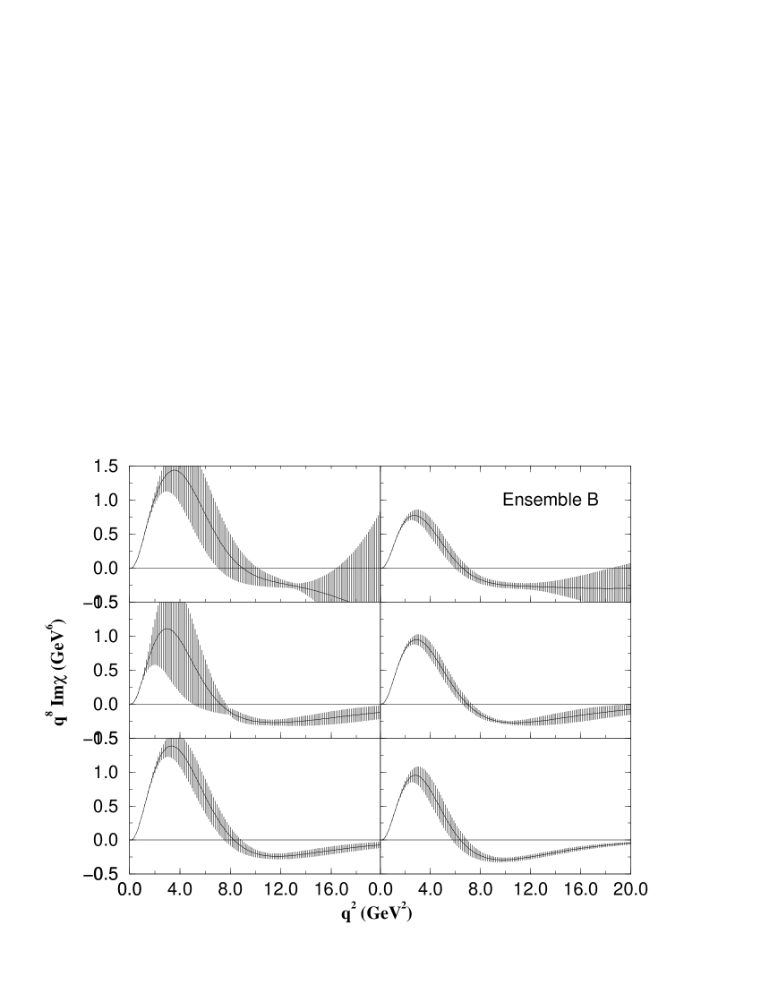
Figure 11: Imaginary part of the Eikonal in the momentum transfer space multiplied by $q^{8}$, obtained by means of the semi-analytical method and ensembles A and B for $pp$ scattering. The energies are the same as indicated in Fig. 10.

Figure 11 shows clearly the role and the effect of data at large values of the momentum transfer. In fact, within the uncertainties, ensemble A shows evidence for the change of sign only at $\sqrt{s}$ = 44.7 GeV and 52.8 GeV, which correspond to the sets with the largest $q^{2}$ interval with available data (see Fig. 3). On the other hand, with ensemble B, we find statistical evidence for the change of sign at all the energies investigated. From these plots we can determine the position of the zeros and the associated errors from the extrems of the uncertainty region (in general not symmetrical). The position of the zero can also be obtained from the numerical method (Fig. 10), but without uncertainties.

In the case of $\bar{p}p$ scattering the semi-analytical method does not provide any evidence for change of sign as illustrated in Figs 12, 13 and 14. As mentioned before, the $pp$ data at $\sqrt{s}$ = 27.5 GeV are not statistically consistent with the $\bar{p}p$ data and, for this reaction, the regions with available data are very small, $q^{2}<$ 4.5 GeV².

Figure 12: Imaginary part of the Eikonal in the momentum transfer space multiplied by $q^{8}$, obtained by means of the numerical and the semi-analytical methods with ensemble A for $\bar{p}p$ scattering at 19.5 GeV.

Figure 13: Imaginary part of the Eikonal in the momentum transfer space multiplied by $q^{8}$, obtained by means of the numerical and the semi-analytical methods with ensemble A for $\bar{p}p$ scattering at 53 GeV.

Figure 14: Imaginary part of the Eikonal in the momentum transfer space multiplied by $q^{8}$, obtained by means of the numerical and the semi-analytical methods with ensemble A for $\bar{p}p$ scattering at 546 GeV.

We conclude that only the $pp$ data from ensemble B provide statistical evidence for change of sign. The results obtained with both methods are shown in Fig. 15. We observe a systematic difference in the position of the zeros as obtained with the numerical and the semi-analytical methods, the former giving values about 0.9 GeV² below those obtained with the later. As the energy increases from 19.5 GeV to 62.5 GeV, the position of the zero decreases from 8.2 to 5.7 GeV² with the numerical method and from 8.9 to 6.4 GeV² with the semi-analytical method. Although the decreasing is not smooth, the general trend, with both methods, favor that behavior, indicating that the position of the zero decreases as the energy increases.

Figure 15: Position of the eikonal zeros in the momentum transfer space as function of the energy, for $pp$ elastic scattering in the interval $19.5-62.5$ GeV: semi-analytical method (with errors) and numerical method (without errors). The lines connecting the points have been drawn only to stress the general trend.

As will be discussed, another quantity of interest is the value of the imaginary part of the eikonal at $q^{2}$ = 0. In this case, all the results obtained with ensembles A and B and through both numerical and semi-analytical methods are exactly the same for the central values (the numerical method does not provide the uncertainties). The results from $pp$ and $\bar{p}p$ scattering are shown in Fig. 16 and will be discussed in Sec. 6.3. Here we only note that the general dependence of $\chi_{I}(s,q)$ on the energy from $pp$ and $\bar{p}p$ scattering, is similar to the behavior of the total cross sections, $\sigma_{tot}^{pp}(s)$ and $\sigma_{tot}^{\bar{p}p}(s)$. In fact that is expected since, in first order, Eq. (1) reads $F_{I}(s,q)\approx\chi_{I}(s,q)$ and, from the optical theorem, $\sigma_{tot}(s)=4\pi F_{I}(s,q=0)$. We shall return to this point in Sec. 6.1.

Figure 16: Imaginary part of the eikonal at $q=0$ for $pp$ and $\overline{p}p$ scattering as function of the energy.

6 Discussion

Our main novel results are displayed in Figs. 11, 15 and 16, and refer, respectively, to the behavior of the eikonal in the $q^{2}$ - space (semi-analytical method), the position of the zero as function of the energy and the eikonal at $q^{2}$ = 0. In this Section we discuss the applicability of these results in the phenomenological context, in connection with those obtained by other authors.

First, we must note that to find a clear dynamical origin for these “empirical” properties of the eikonal is obviously a very difficult task. For that reason, we shall consider here a particular framework, which, despite its simplicity, is suitable for the kind of points we are interested to raise. We shall refer to the Multiple Diffraction Theory by Glauber glauber ; gv , the Chou-Yang model chouyang and the impact picture by Bourrely, Soffer and Wu bsw ; bsw80 ; bsw02 . We understand that the essential ideas to be discussed may be extended to more realistic or general approaches and, in fact, as we shall show, some limited connections with nonperturbative QCD may also be inferred. The discussion will be based on the above three aspects, namely the eikonal zeros, the eikonal at large $q^{2}$ and the eikonal at $q^{2}$ = 0.

6.1 Eikonal zeros

Let us discuss our results concerning the evidence of the eikonal zero and its dependence on the energy in the phenomenological context. We stress that we shall consider simple approaches, so that some important questions may be raised and/or discussed without the influence of “technical” details.

Let us consider the Multiple Diffraction Theory by Glauber. For the scattering between hadrons $A$ and $B$ the eikonal is given by glauber ; gv ; m03

$$\chi(s,q)=\sum_{i=1}^{N_{A}}\sum_{j=1}^{N_{B}}G_{A}G_{B}f_{ij},$$

where $G_{A}$ and $G_{B}$ are the hadronic form factors, $N_{A}$ and $N_{B}$ the number of constituents in each hadron and $f_{ij}$ the individual elementary scattering amplitudes between constituents (parton-parton scattering amplitudes). If we consider, for simplicity, that the elementary amplitudes are all the same, denoted by $f$, and that $N_{A}N_{B}\equiv N$, for $pp$ scattering we have for the imaginary parts

$$\chi_{I}(s,q)=NG_{p}^{2}\ f_{I}.$$ (26)

This expression indicates that, in principle, the zero in the imaginary part of the eikonal may be associated either with the form factor or with the elementary amplitude. Let us discuss both possibilities.

In the phenomenological context (multiple diffraction models), the interpretation of the zero as associated with the elementary amplitude has been discussed, for example, in m03 . On the other hand, more recently, elementary amplitudes have been determined from nonperturbative QCD mmt ; mm03 , by means of the Stochastic Vacuum Model svm . The fundamental input is the gluon gauge-invariant two-point correlation functions, which eventually determines the structure of the elementary amplitude. Two variants may be found in the literature, which can be distinguished by the behavior of the correlators in the region of small (physical) distances. From lattice QCD, in both quenched approximation (absence of fermions) and full QCD (dynamical fermions included), the parametrized correlator has a divergent term, $1/x^{4}$, at the origin digi . In contrast, the parametrization introduced by Dosch, Ferreira and Krämer is finite at the origin dosch . It has been shown in mm03 that the elementary amplitudes determined with the lattice parametrization are characterized by a monotonic decrease of the amplitude with the momentum transfer, through positive values (no zeros). On the other hand, the finite correlator, by Dosch, Ferreira and Krämer, leads to an elementary amplitude which presents a zero at $q^{2}\approx$ 0.5 GeV² (the position of the zero depends on the value of the gluonic correlation length) and then goes asymptotically to zero through negative values mmt . It should be noted that this formalism is intended for asymptotic energies ($s\rightarrow\infty$) and small momentum transfer (typically $q^{2}\leq{\cal O}(1)$ GeV²), which put some limitations in the conclusions that may be inferred, as discussed in detail in mmt ; mm03 . It has been claimed that the divergent term in the correlator is a perturbative effect that should not be included in nonperturbative calculations. However, since there is no conclusive answer to this question in the literature, the possibility that the elementary amplitudes have no zeros can not be disregarded.

Let us, therefore, consider the possibility that the eikonal zero is associated with the form factor, that is, assuming the positivity of the elementary amplitude as in the case of the parametrization from lattice QCD mm03 . In that case, a striking result is the dependence of the position of the eikonal zero on the energy. From a “pragmatic” or “empirical” point of view, for $pp$ and $\bar{p}p$ hadronic elastic scattering, that dependence may be associated with the shrinkage of the diffraction peak, an effect experimentally verified when the energy increases in the region 23 GeV $\leq\sqrt{s}\leq$ 1.8 TeV matthiae . In fact, as recalled before, in first order, $F_{I}(s,q)\approx\chi_{I}(s,q)$ and, as it is known, the diffraction peak is dominated by the imaginary part of the amplitude. This possibility brings novel insights, since the main point is the implication in hadronic form factors depending on the energy, which is an old phenomenological conjecture. Despite of limited theoretical foundation, it has been shown, in the past, that the introduction of energy dependence in form factors leads to good descriptions of the experimental data gofs ; bcmp . In particular, $pp$ and $\bar{p}p$ elastic scattering data can be well described by means of both geometrical models menon and hybrid Regge-dual models covo . We understand that to explore this dependence in well founded theoretical grounds (with analyticity and crossing taken explicitly into account) may lead to novel results in the investigation of the soft diffractive processes in general.

As commented in kawa2 , the eikonal zero may indicate the existence of two components in the hadronic elastic process, one dominating the region of small momentum transfer (long range) and the other the region of large momentum transfer (short range). Roughly, these components could be associated with the regions before and after the position of the zero, respectively. If that is the case the characteristic of the long range component is the positivity of the eikonal in the $q^{2}$ - space, in contrast with its negative values in the short range region. We shall discuss this later case in the following Subsection.

All the previous discussion was based on high-energy hadronic interactions ($pp$ elastic scattering) and, therefore, the form factor concerns the hadronic structure of the proton. To end this subsection, let us discuss some results recently obtained from experiments on elastic electron-proton scattering and related to the electromagnetic structure of the proton. Although, presently, discrepancies from two different experimental techniques characterize the results, future experimental and theoretical developments may bring new insights on possible connections between hadronic and electromagnetic form factors, as discussed in what follows.

The experiments on elastic $e-p$ scattering provide information on the ratio $R\equiv\mu_{p}G_{Ep}(q^{2})/G_{Mp}(q^{2})$, where $G_{Ep}(q^{2})$ and $G_{Mp}(q^{2})$ are the Sachs electric and magnetic form factors and $\mu_{p}$ the proton magnetic moment. The traditional method used to extract the form factors is based on the Rosenbluth separation technique rose and fits to data on $R$, as function of the momentum transfer, have yielded a scaling behavior: $R\approx 1$ scaling1 .

Recently, this ratio has been measured at the Jefferson Laboratory by means of the polarization transfer technique ($\vec{e}p\rightarrow e\vec{p}$) and the results indicated a decrease of the ratio from 0.97 to 0.27, as the momentum transfer increases from 0.5 to 5.5 GeV² (nonscaling behavior) jones ; gayou1 ; gayou2 . Extrapolation from empirical fits indicates a zero (change of sign) at $q^{2}\approx$ 7.7 GeV² gayou2 and a recent phenomenological description of these data, in the context of a Regge parametrization for Generalized Parton Distributions yielded a zero in the electric form factor at $q^{2}\approx$ 8 GeV² guidal . Certainly, these results suggest some possible connections between the inferred position of the zero in the electric form factor and the position the eikonal zeros at $q^{2}\approx$ 6 - 9 GeV² (Figure 15), which, as discussed before, may be associated with the hadronic form factor.

However, new measurements performed at Jefferson Lab through the Rosenbluth technique have confirmed the scaling behavior christy and the same result has been obtained in more recent and improved measurements qattan : global analysis of the cross section data indicates $R\approx 1$ in the momentum-transfer region $q^{2}$: 0 - 6 GeV².

As discussed in qattan , despite the inconsistency of the results in the region of large momentum transfer, both measurements (polarization transfer and improved Rosenbluth) are of comparable precision and the origin of the discrepancy is not clear yet (see qattan for references on possible theoretical corrections in development).

Certainly this enigma must be explained before any attempt to conclude on the existence or not of a zero in the electric form factor at $q^{2}\approx$ 7 - 8 GeV². However, in case that further experimental and/or theoretical developments might favor the polarization-transfer form factors qattan , it may be important to investigate possible connections between zeros in the electric and hadronic form factors.

6.2 Eikonal at large $q^{2}$

Figure 11 (and also 10) shows another interesting aspect of the extracted eikonal, in the region of intermediate and large momentum transfer. The results indicate that, after the zero, the eikonal reaches a minimum and then approaches zero through negative values. That may indicate a second asymptotic zero, which is obviously expected as $q^{2}\rightarrow\infty$. However, this approximation to zero through negative values brings some new insights in model constructions.

For example, let us return to the impact picture by Bourrely, Soffer and Wu. In this model, the contribution from the Pomeron exchange is assumed to be factorized in $s$ and $b$, with the impact parameter dependence given by the parametrization (11) for the form factors in the $q^{2}$ - space. Since, as $q^{2}\rightarrow\infty$, $G(q)\rightarrow$ 0 and $f_{\mathrm{BSW}}(q)\rightarrow-$ 1, this parametrization qualitatively reproduces the change of sign in the eikonal and the limit to zero through negative values. However, as quoted before, the position of the zero fixed at $a^{2}=$ 3.45 GeV² bsw02 is in disagreement with our extracted behavior.

It should be noted that this model overestimates the differential cross section data in the region of large momentum transfer bsw ; bsw02 , a point also raised in kawa2 . If this effect is not only a consequence of the above factorized Pomeron contributions, it may be associated with the behavior of the eikonal after the zero, as mentioned before, that is, the short range contribution. In this case, it may be recalled that a modified BSW factor (mBSW), given by

$$f_{\mathrm{mBSW}}(q)=\frac{1-q^{2}/a^{2}}{1+q^{4}/a^{4}},$$ (27)

can also generate the above behavior of the eikonal and leads to good descriptions of the experimental data at large momentum transfer. This function has been introduced in bcmp and used in both the geometrical approach (with $a^{2}$ = 8.2 GeV²) menon and a hybrid Regge-dual model covo . The differences between these two ansatz are illustrated in Fig. 17 for the position of the zero at $a^{2}=$ 3.45 GeV².

We understand that tests with both functions, taking into account the possibility that the parameter $a^{2}$ depends on the energy may lead to improved descriptions of the experimental data. We are presently investigating this subject.

Figure 17: The Bourrely-Soffer-Wu term, from Eq. (11), and the modified form, Eq. (28), as function of the momentum transfer and for $a^{2}$ = 3.45 GeV².

6.3 Eikonal at $q^{2}$ = 0

Figure 16 shows the imaginary part of the eikonal at $q^{2}=0$, as obtained with both the numerical and semi-analytical methods. As in the previous Subsections, we discuss here some simple examples concerning the applicability of these results in the phenomenological context.

Let us return to the Glauber model, expressed by Eq. (26). Since at $q^{2}=0$ the hadronic form factors are normalized by $G_{p}$ = 1, the dependence on the energy from the imaginary part of the eikonal at $q^{2}=0$ may be associated either with the number of participants constituents or with the elementary amplitude, or both. Only to treat a toy example, let us assume $N=N_{A}$ x $N_{B}$ fixed at 3 x 3 = 9 and consider the Optical Theorem at the elementary level, namely $\sigma_{elem}(s)=4\pi f_{I}(s,q=0)$. In that case we can express the elementary cross section in terms of the imaginary part of the eikonal:

$$\sigma_{elem}(s)=\frac{4\pi}{N}\chi_{I}(s,q=0).$$ (28)

The values of the elementary cross sections, obtained through this formula, with $N$ = 9, from the extracted values of the eikonal at $q^{2}$ = 0, are displayed in Table 4. We see that even with this toy model and for fixed $N$ = 9, the elementary cross sections at the ISR energy region, from analysis of both $pp$ and $\bar{p}p$ scattering, is of the order of 5 - 6 $mb$, a reasonable estimation of the partonic cross sections. Parametrizations of these cross sections as function of the energy have been discussed in cmmm .

In this simple example, we considered the number $N$ of participants in the elementary scattering as fixed. However, in principle, this number may also depend on the energy and, for example, for a fixed elementary cross section (typically 5 - 6 mb) the increase in $\chi_{I}(s,q=0)$ may be associated with an increase of $N$. These considerations are aimed only to exemplify some possible uses of the extracted eikonal. To go on with this discussion demands, however, a more realistic formalism.

Table 4: Elementary (parton-parton) cross sections from $pp$ and $\bar{p}p$ scattering, Eq. (28). The errors come from the uncertainties in the extracted values of $\chi_{I}(s,q=0)$ through the semi-analytical method.

$\sqrt{s}$	$\sigma_{elem}^{pp}$	$\sigma_{elem}^{\bar{p}p}$
(GeV)	(mb)	(mb)
13.8	5.50$\pm$0.05	6.12$\pm$0.02
19.4	5.57$\pm$0.02	5.96$\pm$0.08
23.5	5.48$\pm$0.07	-
30.7	5.71$\pm$0.03	6.05$\pm$0.02
44.7	5.95$\pm$0.03	-
52.8	6.07$\pm$0.02	6.01$\pm$0.18
62.5	6.14$\pm$0.07	5.99$\pm$0.26
546.0	-	9.85$\pm$0.18
1800.0	-	14.53$\pm$0.14

7 Conclusions and final remarks

In this work we have presented the results of analytical fits to $pp$ and $\bar{p}p$ differential cross section data, in a model independent way. As explained, we were not interested in the dependence of the fit parameters with the energy, but only in the best statistical results, in a model-independent context.

By means of both a numerical and a semi-analytical methods, we have determined the imaginary part of the eikonal in the momentum-transfer space. Based on the confidence region of the statistical results, we conclude that the eikonal presents a zero and that the position of the zero, roughly, decreases from 8.5 GeV² to 6.0 GeV² as $\sqrt{s}$ increases from 20 to 60 GeV. After the zero, the eikonal has a minimum and then goes to zero through negative values.

We have presented a critical review on several aspects related to analytical fits to the differential cross section data and also discussions on the applicability of our results in the phenomenological context. Although limited to very simple models, we understand that these aspects may be extended to more realistic approaches.

As discussed, in the phenomenological context, the positivity of the elementary amplitudes determined from quenched and full QCD mm03 suggests that the eikonal zero might be associated with the hadronic form factor. In that case, the decrease in the position of the zero as the energy increases (Figure 15) implies in hadronic form factors depending on the energy. We understand that investigation of this possibility on well founded theoretical bases may lead to important developments in the treatment of the soft diffractive processes.

We have also called the attention to the fact that the position of the eikonal zeros are consistent with the results for the electromagnetic form factor obtained from polarization-transfer experiments. It is expected that the discrepancies between the Rosembluth and polarization-transfer form factors may be resolved in the near future qattan .

As we have shown, only data at large values of the momentum transfer can provide precise answers on the topical question related with the eikonal zeros and their dependence on the energy. In that sense, it would be very important if the experiments at RHIC and LHC could extend the region of momentum transfer to be investigated; as stated in kawa2 : “Such experiments will give much more valuable information for the diffraction interaction rather than to go to higher energies”.

- (1) Y. Dokshitzer, Philos. Trans. R. Soc. London A 359, 309 (2001).
- (2) V. Barone, E, Predazzi, High-Energy Particle Diffraction (Spring-Verlag, Berlin, 2002). E. Predazzi, in International Workshop on Hadron Physics 98, Florianópolis, 1998, edited by E. Ferreira, F.F.S. Cruz, S.S. Avancini (World Scientific, Singapore, 1999) p.80.
- (3) A. Martin, in Proceedings of the VIIIth Blois Workshop - International Conference on Elastic and Diffractive Scattering, Protvino, 1999, edited by V.A. Petrov and A.V. Prokudin (World Scientific, Singapore, 2000) p. 121.
- (4) G. Matthiae, Rep. Prog. Phys. 57, 743 (1994).
- (5) P. Valin, Phys. Rep. 203, 233 (1991).
- (6) R.J. Glauber, in Lectures in Theoretical Physics, edited by W. E. Brittin et al. (Interscience, New York, 1959) Vol. I, p.315; W. Czyż and L.C. Maximom, Ann. Phys. (N.Y.) 52, 59 (1969); V. Franco and G.K. Varma, Phys. Rev. C 18, 349 (1978).
- (7) R. Henzi and P. Valin, Nucl. Phys. B 148, 513 (1979).
- (8) N. Byers, C.N. Yang, Phys. Rev. 142, 976 (1966); T.T. Chou and C.N. Yang, in High Energy Physics and Nuclear Structure, edited by G. Alexander (North-Holland, Amsterdam, 1967) p. 348; Phys. Rev. 170, 1592 (1968); Phys. Rev. Lett. 20, 1213 (1968); Phys. Rev. 175, 1832 (1968).
- (9) R. J. Glauber and J. Velasco, Phys. Lett. B 147, 380 (1984).
- (10) C. Bourrely, J. Soffer and T.T. Wu, Phys. Rev. D 19, 3249 (1979); Nucl. Phys. B 247, 15 (1984); Phys. Rev. Lett. 54, 757 (1985).
- (11) Y. Afek, C. Leroy, B. Margolis, and P. Valin, Phys. Rev. Lett. 45, 85 (1980); L. Durand and H. Pi, Phys. Rev. D 38, 78 (1988).
- (12) M.M. Block, E.M. Gregores, F. Halzen, G. Pancheri, Phys. Rev. D 58, 017503 (1998); 60, 054024 (1999).
- (13) P.A.S. Carvalho e M.J. Menon, Phys. Rev. D 56, 7321 (1997).
- (14) M. Kawasaki, T. Maehara, M. Yonezawa, Phys. Rev. D 57, 1822 (1998).
- (15) M. Kawasaki, T. Maehara, M. Yonezawa, Phys. Rev. D 67, 012013 (2003).
- (16) F. Pereira, E. Ferreira, Phys. Rev. D 59, 014008 (1998); Phys. Rev. D 61, 077507 (2000).
- (17) A.F. Martini, M.J. Menon e D.S. Thober, Phys. Rev. D 57, 3026 (1998).
- (18) M.M. Islam, Nucl. Phys. B 104, 511 (1976).
- (19) L. Durand III, R. Lipes, Phys. Rev. Lett. 20, 637 (1968).
- (20) V. Franco, Phys. Rev. D 11, 1837 (1975).
- (21) S. Dubnicka, V. A. Meshcheryakov, Nucl. Phys. B 83, 311 (1974).
- (22) C. Bourrely, J. Soffer, T. T. Wu, Z. Phys. C 5, 159 (1980).
- (23) T. Maehara, T. Yanagida, M. Yonezawa, Prog. Theor. Phys. 57, 1097 (1977).
- (24) C. Bourrely, J. Soffer, T. T. Wu, Eur. Phys. J. C 28, 97 (2003).
- (25) S. Sanielevici and P. Valin, Phys. Rev. D 29, 52 (1984).
- (26) U. Amaldi and K. R. Schubert, Nucl. Phys. B 166, 301 (1980).
- (27) C. Furget, M. Buenerd, P. Valin, Z. Phys. C 47, 377 (1990).
- (28) K. R. Schubert, Landolt-Börnstein, Numerical Data and Functional Relationships in Science and Technology, New Series, Vol. I/9a (Springer-Verlag, Berlin, 1979).
- (29) A.S. Carrol et al., Phys. Lett. B 61, 303 (1976); G. Fidecaro et al., Phys. Lett. B 105, 309 (1981).
- (30) L.A. Fajardo et al., Phys. Rev. D 24, 46 (1981); D.S. Ayres et al., Phys. Rev. D 15, 3105 (1977); A.S. Carrol et al., Phys. Lett. 80, 423 (1979); C.W. Akerlof et al., Phys. Rev. D 14, 2864 (1976); R. Rubinstein et al., Phys. Rev. D 30, 1413 (1984).
- (31) C. Augier et al. Phys. Lett. B 316, 448 (1993); N. Amos et al., Phys. Lett. B 128, 343 (1983); G. Carboni et al., Nucl. Phys. B 254, 697 (1985); N. Amos et al., Phys. Lett. B 120, 460 (1983); M. Ambrosio et al., Phys. Lett. B 115, 495 (1982); M. Bozzo et al., Phys. Lett. B 147, 392 (1984); N.A. Amos et al., Phys. Rev. Lett. 68, 2433 (1992); N.A. Amos et al., Phys. Lett. B 243, 158 (1990); A. Breakstone et al., Nucl. Phys. B 248, 253 (1984); M. Bozzo et al., Phys. Lett. B 147, 385 (1984); A. Breakstone et al., Phys. Rev. Lett. 54, 2180 (1985); M. Bozzo et al., Phys. Lett. B 155, 197 (1985); D. Bernard et al., Phys. Lett. B 171, 142 (1986).
- (32) R. J. Lombard, C. Wilkin, J. Phys. G 3, L5 (1977).
- (33) T. T. Chou, Found. Phys. 8, 319 (1978).
- (34) H. M. França and Y. Hama, Phys. Rev. D 19, 3261 (1979);
- (35) H. M. França, G. C. Marques, A. J. Silva, Il Nuovo Cimento A 59, 53 (1980).
- (36) C. Bourrely, P. Chiappetta, J. Soffer, T. T. Wu, Phys. Lett. B 132, 191 (1983).
- (37) T. Fearnley, CERN-EP/85-137, 1985 (unpublished).
- (38) R. Lombard, in Proceedings of the First International Workshop on Elastic and Diffractive Scattering, Blois, 1985, edited by B. Nicolescu and J. Tran Thanh Van (Editions Frontieres, Gif-Sur-Yvette, 1986) p. 231.
- (39) H. M. França, Phys. Lett. B 392, 475 (1997).
- (40) B. Z. Kopeliovich, I. K. Potashnikova, B. Povh, E. Predazzi, Phys. Rev. D 63, 054001 (2001).
- (41) A. Donnachie and P. V. Landshoff, Z. Phys. C 2, 55 (1979); Phys. Lett. B 387, 637 (1996).
- (42) W. Faissler et al., Phys. Rev. D 23, 33 (1981); E. Nagy et al., Nucl. Phys. B 150, 221 (1979).
- (43) F. James and M. Roos, Minuit-Function Minimization and Error Analysis, CERN D506 (CERN, Geneva, 1992);
- (44) P. R. Bevington and D. K. Robinson, Data Reduction and Error Analysis for the Physical Sciences (McGraw-Hill, 1992).
- (45) R. Castaldi, G. Sanguinetti, Ann. Rev. Nucl. Part. Sci. 35, 351 (1985).
- (46) A. Martin, Phys. Lett. B 404, 137 (1997).
- (47) NAG Fortran Library Manual, Mark 16 (1993).
- (48) M.J. Menon, Phys. Rev. D 48, 2007 (1993); A.F. Martini, M.J. Menon, D.S. Thober, Phys. Rev. D 54, 2385 (1996).
- (49) A. F. Martini, M. J. Menon, Phys. Lett. B 570, 53 (2003);
- (50) H. G. Dosch, Phys. Lett. B 190, 177 (1987); H. G. Dosch and Yu. A. Simonov, Phys. Lett B 205, 339 (1988), Yu. A. Simonov, Nucl. Phys. B 307, 512 (1998).
- (51) A. Di Giacomo, E. Meggiolaro, H. Panagopoulos, Nucl. Phys. B 483, 371 (1997); M. D’Elia, A. Di Giacomo, E. Meggiolaro, Phys. Lett. B 408, 315 (1997).
- (52) A. Krämer and H. G. Dosch, Phys. Lett. B 252, 669 (1990); H. G. Dosch, E. Ferreira and A. Krämer, Phys. Rev. D 50, 1992 (1994).
- (53) B. Carreras, J. N. J. White, Nucl. Phys. B 42, 95 (1972); J. N. J. White, Nucl. Phys. B 51, 23 (1973); J. Bellandi et al., Hadronic J. 10, 95 (1987); 10, 149 (1987); T. T. Chou and C. N. Yang, Phys. Lett. B 244, 113 (1990).
- (54) J. Bellandi, R.J.M. Covolan, M.J. Menon, B.M. Pimentel, Hadronic J. 11, 17 (1988).
- (55) M.J. Menon, Doctoral Thesis, Instituto de Física Gleb Wataghin, Universidade Estadual de Campinas, 1988; Nucl. Phys. B (Proc. Suppl.) 25, 94 (1992); Canadian J. Phys. 74, 596 (1996).
- (56) R.J.M. Covolan, L.L. Jenkovszky, E. Predazzi, Z. Phys. C, 51, 459 (1991); R.J.M. Covolan, P. Desgrolard, M. Giffon, L.L. Jenkovszky, E. Predazzi, Z. Phys. C 58, 109 (1993).
- (57) M.N. Rosenbluth, Phys. Rev. 79, 615 (1950).
- (58) R.C. Walker et al., Phys. Rev. D 49, 5671 (1994).
- (59) M. K. Jones et al., Phys. Rev. Lett. 84, 1398 (2000).
- (60) O. Gayou et al., Phys. Rev. C 64, 038202 (2001).
- (61) O. Gayou et al., Phys. Rev. Lett. 88, 092301 (2002).
- (62) M. Guidal, M.V. Polyakov, A.V. Radyushkin, M. Vanderhaeghen, hep-ph/0410251.
- (63) M.E. Christy et al., Phys. Rev. C 70, 015206 (2004).
- (64) I.A. Qattan et al., nucl-ex/0410010.
- (65) P.A.S. Carvalho, A.F. Martini, M.J. Menon, A.E. Motter, in International Workshop on Hadron Physics 98, Florianópolis, 1998, edited by E. Ferreira, F.F. de Souza Cruz and S.S. Avancini (World Scientific, Singapore, 1999) p. 326.