We discuss hadronic light-by-light scattering contribution to the muon anomalous magnetic moment $a_{\mu}^{\rm lbl}$, paying particular attention to the consistent matching between the short- and the long-distance behavior of the light-by-light scattering amplitude. We argue that the short-distance QCD imposes strong constraints on this amplitude overlooked in previous analyses. We find that accounting for these constraints leads to approximately $50\%$ increase in the central value of $a_{\mu}^{\rm lbl}$, compared to existing estimates. The hadronic light-by-light scattering contribution becomes $a_{\mu}^{\rm lbl}=136(25)\times 10^{-11}$, thereby shifting the Standard Model prediction closer to the experimental value.

Hadronic light-by-light scattering contribution
to the muon anomalous magnetic moment revisited

I Introduction

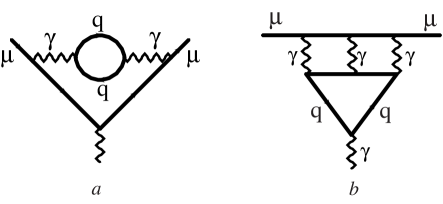
Recent results g-2recent from the experiment E821 at BNL might indicate a disagreement between the experimental value of the muon anomalous magnetic moment $a_{\mu}=(g_{\mu}-2)/2$ and the theoretical expectation based on the Standard Model (SM). Although no definite conclusion is possible at the moment, the experimental value of $a_{\mu}$ is persistently higher than the SM prediction; the significance of the deviation depends on subtle aspects of the low-energy hadronic physics. The largest hadronic contribution to $a_{\mu}$ is due to vacuum polarization, see Fig. 1a.

Figure 1: Hadronic contributions represented by quark loops: ($a$) vacuum polarization, ($b$) light-by-light scattering.

It can be found by integrating the $\sigma(e^{+}e^{-}\to{\rm hadrons})$ annihilation cross-section with the weight function computed in perturbation theory. Experimentally, the $e^{+}e^{-}$ annihilation cross section is obtained either from direct measurements at low energies or, using the isospin symmetry, from hadronic decays of the $\tau$ meson.

The most recent study eidelman gives different results for the $e^{+}e^{-}$– based and the $\tau$– based analyses; the primary reason is the disagreement between the $e^{+}e^{-}$ and the $\tau$ data in the energy range $0.85-1.0~{}{\rm GeV}$. It is this experimental issue that currently limits precision in computing hadronic vacuum polarization contribution to $a_{\mu}$.

Another source of hadronic contributions to $a_{\mu}$ is the light-by-light scattering, induced by hadrons, see Fig. 1b. Compared to the vacuum polarization, this contribution is significantly smaller; nevertheless, given experimental precision on $a_{\mu}$, it is quite important.

The hadronic light-by-light scattering contribution cannot be related to experimental data; for this reason the existing estimates of this contribution are model dependent. This feature leads to major problems in estimating both the central value and the theoretical uncertainty. Given the fact that at low energies the physics of light-by-light scattering is non-perturbative, it is naïve to expect the fully model-independent solution. The satisfactory solution should involve a mixture of both model-dependent and first-principles based considerations in such a way that the uncertainty caused by the model dependence can be minimized and controlled.

To quantify the quality of the low-energy hadronic model, we need a theoretical parameter. Since the perturbation theory is not an option, we must look for the parameter other then the QCD coupling constant. The two possibilities are the smallness of the chiral symmetry breaking and the large number of colors $N_{c}$. The relevance of these parameters can be seen from the parametrical expression for $a_{\mu}^{\rm lbl}$,

$$a_{\mu}^{\rm lbl}\sim\left(\frac{\alpha}{\pi}\right)^{3}\left[c_{1}\,\frac{m_{\mu}^{2}}{m_{\pi}^{2}}+c_{2}N_{c}\,\frac{m_{\mu}^{2}}{\Lambda_{\rm QCD}^{2}}\right],$$ (1)

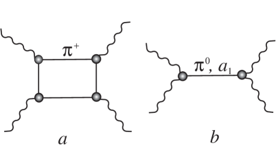
where it is assumed that $m_{\pi}>m_{\mu}$. Only the power dependence on $m_{\pi}^{2}$ is shown; possible chiral logarithms are included into the coefficients $c_{1,2}$. The first, chirally enhanced, term is due to the loops of charged pions in the light-by-light scattering, Fig. 2a. The second, $N_{c}$-enhanced, term is due to exchanges of neutral pion or heavier resonances, Fig. 2b.

Figure 2: Hadronic contributions to the light-by-light scattering: ($a$) charged pion loop, ($b$) exchange of neutral pion and other resonances.

At first sight, it seems natural to expect the chiral parameter $m_{\pi}^{2}/(4\pi f_{\pi})^{2}$ to be a better expansion parameter for $a_{\mu}^{\rm lbl}$. However, a more careful analysis indicates that things can, and perhaps do, work differently. In particular, in all hadronic models used to estimate $a_{\mu}^{\rm lbl}$, the chirally enhanced two-pion contribution is always much smaller than the color enhanced contribution. We present the “anatomy” of the chirally enhanced ${\cal O}(N_{c}^{0})$ contribution in the last Section of this paper where we argue that this smallness may not be accidental.

Moreover, a similar example is provided by the hadronic vacuum polarization contribution to $a_{\mu}$. There, the chirally enhanced two-pion contribution gives approximately $3\times 10^{-9}$ which should be compared with the $N_{c}$-enhanced contribution due to the $\rho$-meson that gives approximately $50\times 10^{-9}$. Although we do not have a clear understanding of why the chirally enhanced terms are subdominant to such an extent, the above arguments suggest that we should accept the dominance of the large-$N_{c}$ expansion over the chiral expansion as the working hypothesis. The special feature of the large-$N_{c}$ limit is that scattering amplitudes in any particular channel are given by infinite sums of narrow resonances. This helps in constructing the model but is clearly insufficient; we need further constraints to select among prospective models.

Such constraints come from the knowledge of short-distance behavior of the light-by-light scattering amplitude, governed by QCD. The asymptotics of this amplitude at large Euclidean photon momenta is derived from the operator product expansion (OPE). The leading term in this OPE comes from the quark box diagram enhanced by large $N_{c}$. This shows a consistency of the OPE constraints with the large-$N_{c}$ limit. Therefore, we require an acceptable large-$N_{c}$ hadronic model, extrapolated to large Euclidean photon momenta, to match the perturbative light-by-light scattering amplitude. We find that the minimal large-$N_{c}$ model which satisfies this criterion includes exchanges of the pseudoscalar $0^{-}$ mesons $\pi^{0},\eta,\eta^{\prime}$ and the the pseudovector $1^{+}$ resonances $a_{1},f_{1},f_{1}^{*}$ . It is important to emphasize at this point that the model with a finite number of resonances is consistent with the short-distance constraints for $a_{\mu}^{\rm lbl}$; it is known that this is not always the case ( see BGLP for a recent discussion).

The short-distance QCD constraints are most restrictive in the pseudoscalar isovector channel. In a special kinematic limit, where invariant masses of two virtual photons are much larger than the invariant mass of the third photon, this channel is completely saturated by the neutral pion. The saturation is complete in the sense that it works for arbitrary small invariant mass of the third virtual photon, in spite of the fact that, in general, the OPE applies only when that mass is much larger than $\Lambda_{\rm QCD}$.

This happens because in the kinematic limit described above, the OPE relates hadronic light-by-light scattering diagram to the famous “anomalous” triangle diagram with one axial and two vector currents. Because both perturbative and non-perturbative corrections to the anomalous triangle are absent in the limit of exact chiral symmetry, the pion pole contribution is unambiguous both at small $q\sim\Lambda_{\rm QCD}$ and at large $q\gg\Lambda_{\rm QCD}$ momenta. This observation connects the two regions of momenta and provides an important constraint thereby.

In terms of the diagram in Fig. 2a, the constraint amounts to the statement that the form factor is present in the $\pi\gamma^{*}\gamma^{*}$ vertex if both photons are virtual but it is absent if that vertex contains the external magnetic field. Although the pseudoscalar channel has been the subject of many detailed studies in the past, this constraint has been overlooked and, as the result, the $\pi^{0}$-pole contribution to $a_{\mu}$ was underestimated. This is the main source of corrections we find for the pion pole contribution.

Moreover, additional constraints on subleading terms in $\pi\gamma^{*}\gamma^{*}$ form factor, derived long ago in Ref.misuse , were not utilized previously. Accounting for these constraints, also leads to the increase in the result. As a consequence, the central value of the pion pole contribution to $a_{\mu}$ increases by approximately $20\times 10^{-11}$. Similar increases occur for other pseudoscalar ($\eta,\eta^{\prime}$) and pseudovector channels ($a_{1},f_{1},f_{1}^{*}$).

Unfortunately, the constraints on all, but $\pi^{0}$, exchanges are not very restrictive; because of that we cannot claim significant reduction in the theoretical uncertainty of hadronic light-by-light scattering contribution to $a_{\mu}$. Nevertheless, imposing all the constraints from the short-distance QCD, we arrive at $a_{\mu}^{\rm lbl}=136(25)\times^{-11}$ which is approximately $50$ per cent larger than the existing estimates bijnes ; klbl ; klbl2 ; knecht .

The rest of the paper is organized as follows. In the next Section we discuss the constraints coming from the short-distance QCD and a minimal model for hadronic contributions to $a_{\mu}^{\rm lbl}$. We consider the pseudoscalar and the pseudovector exchanges in Sections III and IV, respectively. In Section V we briefly discuss the ${\cal O}(N_{c}^{0})$ pion box contribution to $a_{\mu}^{\rm lbl}$. We present our conclusions in Section VI. Additional formulas are given in Appendices.

II Short-distance QCD constraints and hadronic model

In this Section we describe the constraints coming from the short-distance QCD and formulate the hadronic model that satisfies these constraints.

II.1 Kinematics

We begin with the kinematics. The light-by-light scattering amplitude involves four photons with momenta $q_{i}$ and the polarization vectors $\epsilon_{i}$. We take the photon momenta to be incoming, $\sum q_{i}=0$. The first three photons are virtual, while the fourth one represents the external magnetic field and can be regarded as a real photon with the vanishingly small momentum $q_{4}$. The amplitude ${\cal M}$ is defined as

$${\cal M} = \alpha^{2}N_{c}\,{\rm Tr}\,[{\hat{Q}}^{4}]\,{\cal A}=\alpha^{2}N_{c}\,{\rm Tr}\,[{\hat{Q}}^{4}]\,{\cal A}_{\mu_{1}\mu_{2}\mu_{3}\gamma\delta}\epsilon_{1}^{\mu_{1}}\epsilon_{2}^{\mu_{2}}\epsilon_{3}^{\mu_{3}}f^{\gamma\delta}$$ (2)

$$= -e^{3}\!\int\!{\rm d}^{4}x\,{\rm d}^{4}y\,{\rm e}^{-iq_{1}x-iq_{2}y}\,\epsilon_{1}^{\mu_{1}}\epsilon_{2}^{\mu_{2}}\epsilon_{3}^{\mu_{3}}\langle 0|T\left\{j_{\mu_{1}}(x)\,j_{\mu_{2}}(y)\,j_{\mu_{3}}(0)\right\}|\gamma\rangle,$$

where $j_{\mu}$ is the hadronic electromagnetic current, $j_{\mu}\!=\!\bar{q}\,\hat{Q}\gamma_{\mu}q$, written in terms of the three quark flavors $q\!=\!\{u,d,s\}$ with $\hat{Q}$ being the $3\times 3$ diagonal matrix of quark electric charges. In addition, $f^{\gamma\delta}\!=\!q_{4}^{\gamma}\epsilon_{4}^{\delta}-q_{4}^{\delta}\epsilon_{4}^{\gamma}$ denotes the field strength tensor of the soft photon; the light-by-light scattering amplitude is proportional to this tensor due to gauge invariance. Since ${\cal M}$ is linear in the small momentum $q_{4}$, for the purpose of computing the light-by-light scattering contribution to $a_{\mu}$, we can set $q_{4}=0$ in the tensor amplitude ${\cal A}_{\mu_{1}\mu_{2}\mu_{3}\gamma\delta}$ and calculate it assuming that $q_{1}+q_{2}+q_{3}=0$ for the virtual photons. Because the momenta $q_{1},q_{2},q_{3}$ form a triangle, there are just three independent Lorentz invariant variables; we choose them to be the virtualities of the photons $q_{1-3}^{2}$.

In general, the light-by-light scattering amplitude is a complicated function of photon’s virtualities. However, there are only two distinct kinematic regimes in the light-by-light scattering amplitudes: the Euclidean momenta of the three photons are comparable in magnitude $q_{1}^{2}\sim q_{2}^{2}\sim q_{3}^{2}$, or one of the momenta is much smaller than the other two. The second limit can be analyzed in a very simple fashion using the OPE of the light-by-light scattering. Also, this limit is of importance because it helps us to identify the pole-like structures in the OPE amplitudes and in this way connect the OPE to phenomenological models.

II.2 OPE and triangle amplitude

Since the light-by-light scattering amplitude is symmetric with respect to photon permutations, we can study the second limit assuming that $q_{1}^{2}\approx q_{2}^{2}\gg q_{3}^{2}\,$. In this kinematic regime, we begin with the well-known OPE (see e.g. Bj ) for the product of two electromagnetic currents that carry the largest momenta $q_{1},q_{2}$,

$$i\!\int\!{\rm d}^{4}x\,{\rm d}^{4}y\,{\rm e}^{-iq_{1}x-iq_{2}y}\,T\left\{j_{\mu_{1}}(x),j_{\mu_{2}}(y)\right\}=$$

$$\int\!{\rm d}^{4}z\,{\rm e}^{-i(q_{1}+q_{2})z}\,\frac{2i}{{\hat{q}}^{2}}\,\epsilon_{\mu_{1}\mu_{2}\delta\rho}\,{\hat{q}}^{\delta}j_{5}^{\rho}(z)+\cdots\,.$$ (3)

Here, $j^{\rho}_{5}=\bar{q}\,\hat{Q}^{2}\gamma^{\rho}\gamma_{5}\,q$ is the axial current, where different flavors enter with weights proportional to squares of their electric charges and $\hat{q}=(q_{1}-q_{2})/2\approx q_{1}\approx-q_{2}\,$. We retain only the leading (in the limit of large Euclidean $\hat{q}$) term in the OPE associated with the axial current $j_{5}^{\rho}$; the ellipsis in Eq.(II.2) stands for subleading terms suppressed by powers of $\Lambda_{\rm QCD}/\hat{q}$. The momentum $q_{1}+q_{2}=-q_{3}$ flowing through $j^{5}_{\rho}$ is assumed to be much smaller than $\hat{q}$. We note in passing that Eq.(II.2) has been applied earlier in various situations; for example, the matrix element of Eq.(II.2) between the pion and the vacuum states gives the asymptotic behavior of the $\pi^{0}\gamma^{*}\gamma^{*}$ amplitude at large photon virtualities misuse .

For the purpose of further discussion it is convenient to present the current $j_{5\rho}$ as a linear combination of the isovector, $j_{5\rho}^{(3)}=\bar{q}\lambda_{3}\gamma_{\rho}\gamma_{5}q$, hypercharge, $j_{5\rho}^{(8)}=\bar{q}\lambda_{8}\gamma_{\rho}\gamma_{5}q$, and the SU(3) singlet, $j_{5\rho}^{(0)}=\bar{q}\gamma_{\rho}\gamma_{5}q$, currents,

$$j_{5\rho}=\sum_{a=3,8,0}\frac{{\rm Tr}\,[\lambda_{a}\hat{Q}^{2}]}{{\rm Tr}\,[\lambda_{a}^{2}]}\,j_{5\rho}^{(a)}\,,$$ (4)

where $\lambda_{0}$ is the unity matrix.

Once the dependence on the largest momenta $q_{1,2}$ is factored out, the next step is to find the dependence of the light-by-light scattering amplitude on the momentum $q_{3}$. This dependence is given by the amplitudes $T_{\gamma\rho}^{(a)}$ that involve axial currents $j_{5\rho}^{(a)}$ and two electromagnetic currents, one with momentum $q_{3}$ and the other one (the external magnetic field) with the vanishing momentum

$$T_{\mu_{3}\rho}^{(a)}\!=i\,\langle 0|\!\int\!{\rm d}^{4}z\,{\rm e}^{iq_{3}z}T\{j^{(a)}_{5\rho}(z)\,j_{\mu_{3}}(0)\}|\gamma\rangle.$$ (5)

The triangle amplitudes for such kinematics were considered recently in CMV . It is shown in that reference that $T_{\gamma\rho}^{(a)}$ can be written through two independent amplitudes,

$$T_{\mu_{3}\rho}^{(a)}=-\frac{ie\,N_{c}{\rm Tr}\,[\lambda_{a}\hat{Q}^{2}]}{4\pi^{2}}\left\{w^{(a)}_{L}\!(q_{3}^{2})\,q_{3\rho}q_{3}^{\sigma}\tilde{f}_{\sigma\mu_{3}}+\right.$$

$$\left.+w^{(a)}_{T}\!(q_{3}^{2})\!\left(-q_{3}^{2}\tilde{f}_{\mu_{3}\rho}\!+\!q_{3\mu_{3}}q_{3}^{\sigma}\tilde{f}_{\sigma\rho}\!-\!q_{3\rho}q_{3}^{\sigma}\tilde{f}_{\sigma\mu_{3}}\right)\right\}.$$ (6)

The first (second) amplitude is related to the longitudinal (transversal) part of the axial current, respectively. In terms of hadrons, the invariant function $w_{L(T)}$ describes the exchanges of the pseudoscalar (pseudovector) mesons.

In perturbation theory $w_{L,T}$ are defined by the famous triangle diagram. For massless quarks, we obtain:

$$w^{(a)}_{L}(q^{2})=2w^{(a)}_{T}(q^{2})=-\frac{2}{q^{2}}\,.$$ (7)

An appearance of the longitudinal part is the signature of the axial Adler-Bell-Jackiw (ABJ) anomaly ABJ . Although the perturbation theory is only reliable for $q^{2}\gg\Lambda_{\rm QCD}^{2}$, where it coincides with the leading term of the OPE for the time-ordered product of the axial and electromagnetic currents, the expressions for longitudinal functions $w^{(3,8)}_{L}$ given in Eq.(7) are exact QCD results in the chiral limit $m_{q}=0$ for nonsinglet axial currents. The fact that there are no perturbative adler and nonperturbative thooft corrections to the axial anomaly implies that the pole behavior of $w^{(3,8)}_{L}$ in Eq.(7) is correct all the way down to small $q^{2}$, where the poles are associated with Goldstone pseudoscalar mesons, $\pi^{0}$ in $w^{(3)}_{L}$ and $\eta$ in $w^{(8)}_{L}$.

Equations (6) and (7) allow us to derive the coupling of the $\pi^{0}$ meson to photons. To this end, consider the isovector part of the triangle amplitude $T_{\gamma\rho}^{(3)}$. The residue at $q^{2}=0$, corresponding to the $\pi^{0}$ pole, is the product of two matrix elements,

$$\langle 0|j^{(3)}_{5\rho}|\pi^{0}\rangle=2iF_{\pi}\,q_{\rho}\,,~{}~{}~{}\langle\pi^{0}|j_{\mu_{3}}|\gamma\rangle=-4eg_{\pi\gamma\gamma}q^{\sigma}\tilde{f}_{\sigma\mu_{3}}\,.$$ (8)

Comparing with Eqs.(6), (7) we derive the well-known result ABJ for $\pi\gamma\gamma$ coupling:

$$g_{\pi\gamma\gamma}=\frac{N_{c}{\rm Tr}\,[\lambda_{3}{\hat{Q}}^{2}]}{16\pi^{2}\,F_{\pi}}\,.$$ (9)

In a similar way, the $g_{\eta\gamma\gamma}$ coupling in the chiral limit can be derived, if needed.

The absence of perturbative and non-perturbative corrections and therefore the possibility to use the OPE expressions for vanishing values of $q^{2}$ is unique for the longitudinal part of nonsinglet axial currents. For the transversal functions $w_{T}$ as well as for the singlet longitudinal function $w_{L}^{(0)}$, there are higher order terms in the OPE that, upon summation, generate mass terms that shift the pole position $1/q^{2}\to 1/(q^{2}-m^{2})$. We use this modification of the pole-like terms for each channel in what follows. The lightest pseudovector mesons are the $a_{1}(1260)$, $f_{1}(1290)$ and $f_{1}^{*}(1420)$ mesons. For the singlet axial current the pole in $w_{L}^{(0)}$ is shifted to $m_{\eta^{\prime}}^{2}\,$.

Consider a triangle amplitude for any isospin channel in the limit of large $q^{2}$, where the OPE and the perturbation theory are applicable and Eq.(7) is valid. An important consequence of this equation is that triangle amplitudes are not suppressed for such values of $q^{2}$. In terms of hadrons it means that no form factor is present in the $h\gamma^{*}\gamma$ interaction vertex where the real photon is soft (external magnetic field). This is in clear contradiction with the common practice klbl ; bijnes ; knecht when, for $\pi^{0}$ exchange, the form factor $F_{\pi\gamma^{*}\gamma}(q^{2},0)$ is introduced. Such transition form factor has to be present when one of the photons is virtual, the other photon is on the mass shell and the pion is on the mass shell as well. However, this is not the kinematics that corresponds to the triangle and the light-by-light scattering amplitudes, relevant for $a_{\mu}$ computation, where the pion virtuality is the same as the virtuality of one of the photons. The absence of the suppression is also consistent with the dispersion representation of the amplitude since the imaginary part is nonvanishing only at $q^{2}=0$ in the chiral limit.

Combining Eqs.(II.2-6), we write the the light-by-light amplitude ${\cal A}_{\mu_{1}\mu_{2}\mu_{3}\gamma\delta}$ for $q_{1}^{2}\approx q_{2}^{2}\gg q_{3}^{2}$ in the following form:

$${\cal A}_{\mu_{1}\mu_{2}\mu_{3}\gamma\delta}f^{\gamma\delta}=\frac{8}{{\hat{q}}^{2}}\epsilon_{\mu_{1}\mu_{2}\delta\rho}{\hat{q}}^{\delta}\!\!\sum_{a=3,8,0}\!\!W^{(a)}\left\{w^{(a)}_{L}\!(q_{3}^{2})\,q_{3}^{\rho}q_{3}^{\sigma}\tilde{f}_{\sigma\mu_{3}}+w^{(a)}_{T}\!(q_{3}^{2})\!\left(-q_{3}^{2}\tilde{f}_{\mu_{3}}^{\rho}\!+\!q_{3\mu_{3}}q_{3}^{\sigma}\tilde{f}_{\sigma}^{\rho}\!-\!q_{3}^{\rho}q_{3}^{\sigma}\tilde{f}_{\sigma\mu_{3}}\right)\right\}+\cdots,$$ (10)

where no hierarchy between $q_{3}^{2}$ and $\Lambda_{\rm QCD}^{2}$ is assumed. The weights $W^{(a)}$ are defined as

$$W^{(a)}=\frac{\left({\rm Tr}\,[\lambda_{a}\hat{Q}^{2}]\right)^{2}}{{\rm Tr}\,[\lambda_{a}^{2}]{\rm Tr}\,[\hat{Q}^{4}]}\,;$$ (11)

$$W^{(3)}=\frac{1}{4}\,,\quad W^{(8)}=\frac{1}{12}\,,\quad W^{(0)}=\frac{2}{3}\,.$$

In the limit $q_{3}^{2}\gg\Lambda_{\rm QCD}^{2}$, Eq.(10) can be simplified using the asymptotic expressions Eq.(7) for the invariant functions $w_{L,T}^{(a)}$. Convoluting the tensor amplitude with the photon polarization vectors and analytically continuing to Euclidean space, we arrive at:

$${\cal A}\!=\!\frac{4}{q_{3}^{2}\,\hat{q}^{2}}\{f_{2}\tilde{f}_{1}\}\{\tilde{f}f_{3}\}\!-\!\frac{4}{q_{3}^{2}\,\hat{q}^{4}}\!\left(\!\!\{q_{2}f_{2}\tilde{f}_{1}\tilde{f}f_{3}q_{3}\}\!\right.$$

$$\left.+\!\{q_{1}f_{1}\tilde{f}_{2}\tilde{f}f_{3}q_{3}\}\!+\!\frac{q_{1}^{2}+q_{2}^{2}}{4}\{f_{2}\tilde{f}_{1}\}\{\tilde{f}f_{3}\}\!\!\right)\!+\!\cdots\!.$$ (12)

Here, $f_{i}^{\mu\nu}=q_{i}^{\mu}\epsilon_{i}^{\nu}-q_{i}^{\nu}\epsilon_{i}^{\mu}$ are the field strength tensors, the braces denote either traces of products of the matrices $f_{i}^{\mu\nu}$ or their convolutions with vectors $q_{i}$.

In Eq.(12) and in the remainder of the paper, we use Euclidean notations instead of Minkowski ones used before. The continuation to Euclidean space mostly concerns the change in sign for all $q_{i}^{2}$ and the overall change in sign for the amplitude ${\cal A}$, since it involves the product of two Levi-Cevita tensors. The result can be verified by comparison with the direct computation of the quark box diagram, for arbitrary $q_{1-3}^{2}$, presented in Appendix I. There we show that the amplitude can be described in terms of nineteen independent tensor structures and five independent form-factors. In what follows, we mostly deal with the approximate form of the amplitude Eq.(12), but we make occasional references to general expression in Appendix I.

II.3 The model

Two different terms in Eq.(10) can be identified with exchanges of the pseudoscalar (pseudovector) mesons for the functions $w^{(a)}_{L,T}(q^{2}_{3})$. Extrapolating Eq.(12) from $q^{2}_{1,2}\gg\Lambda_{\rm QCD}^{2}$ to arbitrary $q^{2}_{1,2}$, we arrive at the following model:

$${\cal A}\!=\!{\cal A}_{\rm PS}+{\cal A}_{\rm PV}\,+{\rm permutations},\\$$ (13)

where

$${\cal A}_{\rm PS} \!= \!\!\!\sum_{a=3,8,0}\!\!W^{(a)}\phi^{(a)}_{L}(q_{1}^{2},q_{2}^{2})w_{L}^{(a)}(q_{3}^{2})\{f_{2}\tilde{f}_{1}\}\{\tilde{f}f_{3}\},$$ (14)

$${\cal A}_{\rm PV} \!= \!\!\!\sum_{a=3,8,0}\!\!W^{(a)}\phi^{(a)}_{T}(q_{1}^{2},q_{2}^{2})w_{T}^{(a)}(q_{3}^{2})\left(\!\{q_{2}f_{2}\tilde{f}_{1}\tilde{f}f_{3}q_{3}\}\!+\!\{q_{1}f_{1}\tilde{f}_{2}\tilde{f}f_{3}q_{3}\}\!+\!\frac{q_{1}^{2}+q_{2}^{2}}{4}\{f_{2}\tilde{f}_{1}\}\{\tilde{f}f_{3}\}\!\right).$$ (15)

The form factors $\phi^{(a)}_{L,T}(q_{1}^{2},q_{2}^{2})$ account for the dependence of the amplitude on $q_{1,2}^{2}$. Pictorially (see Fig.2b), these form factors can be associated with the interaction vertex for the two virtual photons on the left hand side, whereas the meson propagator and the interaction vertex on the right hand side form the triangle amplitude described by the functions $w_{L,T}^{(a)}(q_{3}^{2})$. In the next Sections we introduce models for these functions consistent with the short distance behavior of the light-by-light scattering amplitude.

Note that our model does not include explicit exchanges of vector or scalar mesons. This is a consequence of the fact that, to leading order, the OPE of the two vector currents produces the axial vector current only. However, the vector mesons are present in our model implicitly, through the momentum dependence of the form factors $\phi^{(a)}_{L,T}$ as well as the transversal functions $w^{(a)}_{T}$.

III Constraints on the pseudoscalar exchange

The $\pi^{0}$ exchange provides the largest fraction of the hadronic light-by-light scattering contribution to $a_{\mu}$. It is therefore appropriate to scrutinize this contribution as much as possible and ensure that it satisfies all the possible constraints that follow from first principles.

As we discussed earlier, the longitudinal part of the triangle amplitude is fixed by the ABJ anomaly. Accounting for explicit violation of the chiral symmetry given by the small mass of the pion, we derive

$$w_{L}^{(3)}(q^{2})=\frac{2}{q^{2}+m_{\pi}^{2}}\,.$$ (16)

The ABJ anomaly also fixes $\phi_{L}^{(3)}(0,0)$,

$$\phi_{L}^{(3)}(0,0)=\frac{N_{c}}{4\pi^{2}F_{\pi}^{2}}\,,$$ (17)

so that the model for the pion exchange in the light-by-light scattering amplitude takes the form,

$${\cal A}_{\pi^{0}} \!= \!-\frac{N_{c}W^{(3)}}{2\pi^{2}F_{\pi}^{2}}\,\frac{F_{\pi\gamma^{*}\gamma^{*}}(q_{1}^{2},q_{2}^{2})}{q_{3}^{2}+m_{\pi}^{2}}\,\{f_{2}\tilde{f}_{1}\}\{\tilde{f}f_{3}\}$$ (18)

$$+\,\mbox{permutations}\,.$$

The $\pi\gamma^{*}\gamma^{*}$ form factor $F_{\pi\gamma^{*}\gamma^{*}}(q_{1}^{2},q_{2}^{2})$ is defined as

$$F_{\pi\gamma^{*}\gamma^{*}}(q_{1}^{2},q_{2}^{2})=\frac{\phi_{L}^{(3)}(q_{1}^{2},q_{2}^{2})}{\phi_{L}^{(3)}(0,0)}\,.$$ (19)

The comparison with the OPE constraint given by the relevant term in Eq.(10) leads to

$$\lim_{q^{2}\gg\Lambda_{\rm QCD}^{2}}F_{\pi\gamma^{*}\gamma^{*}}(q^{2},q^{2})=\frac{8\pi^{2}F_{\pi}^{2}}{N_{c}\,q^{2}}\,,$$ (20)

which is the correct asymptotics indeed misuse . This means that the neutral pion exchange in Eq.(14) saturates the corresponding short-distance QCD constraint.

This comparison also proves our previous claim that the form factor $F_{\pi\gamma^{*}\gamma}(q_{3}^{2},0)$ cannot be present in the amplitude Eq.(18); if that form factor is introduced, the asymptotics of the light-by-light scattering amplitude becomes $1/q_{3}^{4}$, as opposed to $1/q_{3}^{2}$ behavior that follows from perturbative QCD. This proof is, of course, equivalent to our discussion of the triangle amplitude in Section II.

The absence of the second form factor in the amplitude Eq.(18) distinguishes our approach from all other calculations of the pion pole contribution to $a_{\mu}$ that exist in the literature. As we show below, it has a non-negligible impact on the final numerical result for the pseudoscalar contribution to $a_{\mu}$. Here we note, that the result for the pion pole contribution is expected to increase, because the absence of the second form factor leads to slower convergence of the integrals over loop momenta, making the result larger. As we show below, this is indeed what happens.

Further constraints on the model follow from restrictions on the pion transition form factor $F_{\pi\gamma^{*}\gamma^{*}}$ that were recently reviewed in knecht . For numerical estimates we use their LMD+V form factor

$$F_{\pi\gamma^{*}\gamma^{*}}(q_{1}^{2},q_{2}^{2})=\frac{4\pi^{2}F_{\pi}^{2}}{N_{c}}~{}\frac{q_{1}^{2}q_{2}^{2}(q_{1}^{2}+q_{2}^{2})-h_{2}q_{1}^{2}q_{2}^{2}+h_{5}(q_{1}^{2}+q_{2}^{2})+(N_{c}M_{1}^{4}M_{2}^{4}/4\pi^{2}F_{\pi}^{2})}{(q_{1}^{2}+M_{1}^{2})(q_{1}^{2}+M_{2}^{2})(q_{2}^{2}+M_{1}^{2})(q_{2}^{2}+M_{2}^{2})},$$ (21)

where $M_{1}=769~{}{\rm MeV}$, $M_{2}=1465~{}{\rm MeV}$, $h_{5}=6.93~{}{\rm GeV}^{4}$.

The parameter $h_{2}$ was not determined in Ref.knecht and we can fix it if we notice that it contributes to the $1/q^{4}$ correction to the leading asymptotics of the pion form factor, Eq.(20). Such correction comes from the twist 4 operators in the OPE expansion of the two electromagnetic currents Eq.(II.2). It was analyzed long ago in Ref.misuse using the OPE and the QCD sum rules approaches. The result of such an analysis implies that the coefficient of the ${\cal O}(q^{-4})$ term in the asymptotics of the pion form factor is numerically small; in terms of the parametrization Eq.(21), this means that $h_{2}\approx-10~{}{\rm GeV}^{2}$ has to be chosen. We use this value for numerical estimates in what follows.

Equations (18) and (21) completely specify the model for the pion pole contribution that we use for numerical calculations below. Before going into that, we discuss the sensitivity of the final result to possible modifications of the model.

We denote the structure that multiplies $\{f_{2}\tilde{f}_{1}\}\{\tilde{f}f_{3}\}$ in Eq.(18) as $W^{(3)}G_{2}^{\rm mod}(q_{3}^{2},q_{2}^{2},q_{1}^{2})$. Comparing the $\pi^{0}$-pole exchange amplitude, Eq.(18), to the full light-by-light scattering amplitude (see Appendix I), we find that, for asymptotically large virtualities of the photons, the matching requires

$$G_{2}^{\rm mod}(q_{3}^{2},q_{2}^{2},q_{1}^{2})=G_{2}(q_{3}^{2},q_{2}^{2},q_{1}^{2}).$$ (22)

Consider Eq.(22) in the limit $\Lambda_{\rm QCD}^{2}\ll q_{1}^{2}\ll q_{2}^{2}\sim q_{3}^{2}$. It is easy to see that the left hand side in Eq.(22) develops the $1/q_{1}^{2}$ behavior; from expression for $G_{2}$ in Appendix I it follows that $G_{2}(q_{2}^{2},q_{2}^{2},q_{1}^{2})\approx 1/q_{2}^{2}$ in such kinematic regime. Hence, there is a mismatch between our model and the OPE prediction.

The second option is to consider Eq.(22) in the situation when all the momenta are asymptotically large and equal in magnitude $q_{1}^{2}=q_{2}^{2}=q_{3}^{2}=q^{2}$. In this regime,

$$G_{2}(q^{2},q^{2},q^{2})\approx\frac{8}{3q^{4}},$$ (23)

whereas

$$G_{2}^{\rm mod}(q^{2},q^{2},q^{2})\approx\frac{4}{q^{4}}.$$ (24)

Again, the model fails to describe the OPE constraint perfectly.

Of course, the above failures do not necessary invalidate the model; after all we are interested in the light-by-light scattering contribution to $a_{\mu}$ and various regions of loop momenta contribute differently to the integral. For this reason, we have to investigate if the above mismatches influence the numerical estimate for the pion pole contribution to $a_{\mu}^{\rm lbl}$. To this end, we notice that $G_{2}^{\rm mod}(q_{3}^{2},q_{2}^{2},q_{1}^{2})$ can be modified by adding to it

$$\delta G_{2}^{\rm mod}(q_{3}^{2},q_{2}^{2},q_{1}^{2})=$$

$$\frac{\xi q_{1}^{2}q_{2}^{2}}{(q_{1}^{2}+M_{1}^{2})(q_{1}^{2}+M_{2}^{2})(q_{2}^{2}+M_{1}^{2})(q_{2}^{2}+M_{2}^{2})},$$ (25)

without running into a contradiction with the required pole behavior with respect to $q_{3}^{2}$. After adding $\delta G_{2}^{\rm mod}$, it is easy to see that, by tuning $\xi$, one can either ensure that the pole in $q_{1}^{2}$ is absent or that the asymptotic behavior of $G_{2}^{\rm mod}+\delta G_{2}^{\rm mod}$ becomes consistent with Eq.(23). The two constraints are satisfied for $\xi=-2$ and $\xi=-4/3$, respectively.

We can investigate the importance of these constraints by computing the contribution of $\delta G_{2}^{\rm mod}$ to $a_{\mu}^{\rm lbl}$ for $\xi=1$. Upon doing so, we find that it changes $a_{\mu}^{\pi^{0}}$ by $\approx 0.5\times 10^{-11}$. Hence, regardless of the value of $\xi$, $\delta G_{2}^{\rm mod}$ can be neglected at the current level of precision. We therefore use Eqs.(18,21) as our model for the pion form factor in what follows.

The result for $a_{\mu}^{\pi^{0}}$ with the LMD+V form factor for $h_{2}=-10~{}{\rm GeV}^{2}$, quoted in knecht is $a_{\mu}^{\rm\pi^{0}}=63\times 10^{-11}$. Using the formulas in knecht it is easy to repeat their calculation removing the pion transition form factor that involves the soft photon. In that case, the result becomes $76.5~{}\times 10^{-11}$, a shift in the positive direction. In addition, as we mentioned earlier, we consider the value $h_{2}=-10~{}{\rm GeV}^{2}$ to be preferable because of the OPE constraints on the pion transition form factor. Note, however, that $h_{2}=0$ was used in knecht to derive the central value $58\times 10^{-11}$; compared to that number, our central value is larger by approximately $20\times 10^{-11}$.

A similar analysis for the isosinglet channels leads to the conclusion that these channels are saturated by $\eta$ and $\eta^{\prime}$ mesons; matching to pQCD result suggests that no transition form factor is present for the soft photon interaction vertex in those cases as well. Since these contributions are smaller than that of $\pi_{0}$, we do not use sophisticated models for $\eta$ and $\eta^{\prime}$ transition form factors and estimate them using the simplest possible VMD form factor. The $\eta(\eta^{\prime})\gamma^{*}\gamma^{*}$ interaction vertex is normalized in such a way that the decay widths of these mesons into two photons is correctly reproduced; this allows to account for the $\eta-\eta^{\prime}$ mixing in a simple way.

How good these “experimental” couplings compare to the theoretical expectations based on our model? Because of the $\eta-\eta^{\prime}$ mixing, we expect that the sum of $\eta(\eta^{\prime})\gamma\gamma$ couplings squared is predicted by the model more accurately than each of the couplings separately. We find

$$r=\frac{g_{\eta\gamma\gamma}^{2}+g_{\eta^{\prime}\gamma\gamma}^{2}}{g_{\pi\gamma\gamma}^{2}}=3,$$ (26)

whereas using experimental values for the $\eta(\eta^{\prime})\gamma\gamma$ couplings we arrive at $r=2.5(1)$. Although we use this $20\%$ discrepancy as an error estimate on the $\eta+\eta^{\prime}$ contribution, we note that it rather implies an increase in the result since the agreement between “experimental” and theoretical asymptotics can be improved by adding more pseudoscalar mesons to the model.

Compared to the results quoted in knecht , removal of the second form factor increases the $\eta$ and $\eta^{\prime}$ contributions from approximately $a_{\mu}^{\eta}=a_{\mu}^{\eta^{\prime}}=13\times 10^{-11}$ to $a_{\mu}^{\eta}=a_{\mu}^{\eta^{\prime}}=18\times 10^{-11}$. The sum of the contributions from all pseudoscalar mesons ($\pi^{0},\eta,\eta^{\prime}$) leads to the estimate:

$$a_{\mu}^{\rm PS}=114(10)\times 10^{-11}.$$ (27)

The central value in Eq.(27) is almost 40 percent larger than most of the existing results for $a_{\mu}^{\rm lbl}$ klbl ; bijnes ; knecht . The major effect comes from removing the form factor for the interaction of the soft photon (magnetic field) with the pseudoscalar meson; the necessity to do that unambiguously follows from matching the pseudoscalar pole amplitude to the pQCD expression for the light-by-light scattering.

On the contrary, the error estimate in Eq.(27) is subjective; it is based on the variation of the result when input parameters of the model are varied. It is impossible to defend the exact number for the error estimate in Eq.(27); however, we believe that it adequately describes our current knowledge of the pseudoscalar contribution.

IV Pseudovector exchange

In this Section we discuss the pseudovector exchange amplitude ${\cal A}_{\rm PV}$, Eq.(15). From Eqs. (7), (10), (12), we find the asymptotics of $\phi^{(a)}_{T}$ and $w^{(a)}_{T}$,

$$\lim_{\quad q^{2}\gg\Lambda_{\rm QCD}^{2}}\phi^{(a)}_{T}(q^{2},q^{2})=\frac{-4}{q^{4}},\lim_{\quad q^{2}\gg\Lambda_{\rm QCD}^{2}}w^{(a)}_{T}(q^{2})=\frac{1}{q^{2}}.$$ (28)

As we mentioned earlier, the lightest pseudovector resonances are the $a_{1}$ meson with the mass $M_{a_{1}}=1260~{}{\rm MeV}$, the $f_{1}$ meson, with the mass $M_{f_{1}}=1285~{}{\rm MeV}$ and the $f_{1}^{*}$ meson with the mass $M_{f_{1}^{*}}=1420~{}{\rm MeV}$. The contribution of these mesons to $a_{\mu}^{\rm lbl}$ is cut off at the scales defined by their masses. This suggests that the pole-like singularities in Eq.(12) are shifted from zero to the masses of the corresponding pseudovector and vector mesons. We also remind the reader that $\phi^{(a)}_{T}(q_{1}^{2},q_{2}^{2})$ describes the form factor for the $\gamma^{*}\gamma^{*}\to a_{1}(f_{1})$ transition. Shifting all the poles by the same amount, i.e., neglecting mass differences, we get the simplest possible model consistent with perturbative QCD constraints Eq.(28),

$$\phi_{T}^{(a)}(q_{1}^{2},q_{2}^{2})=-\frac{4}{(q_{1}^{2}+M^{2})(q_{2}^{2}+M^{2})}\,,$$

$$w_{T}^{(a)}(q)=\frac{1}{q^{2}+M^{2}}.$$ (29)

This implies, in particular, that we do not distinguish between different isospin channels.

Although this model is not very realistic, we can use it to derive a simple analytic result which will help us to exhibit the dependence on the mass scale $M$. Assuming that $M\gg m_{\mu}$, we compute the contribution of the pseudovector meson to $a_{\mu}$ and obtain:

$$a_{\mu}^{\rm PV} \!\!\!= \!\!\left(\frac{\alpha}{\pi}\right)^{3}\!\frac{m_{\mu}^{2}}{M^{2}}N_{c}{\rm Tr}\,[{\hat{Q}}^{4}]\left[\frac{71}{192}\!+\frac{81}{16}S_{2}-\!\frac{7\pi^{2}}{144}\right]$$ (30)

$$\!\approx \!1010~{}\frac{m_{\mu}^{2}}{M^{2}}\times 10^{-11}\,,$$

where $S_{2}=0.26043$. Using $M=1300~{}{\rm GeV}$ as an example, we obtain $a_{\mu}^{\rm PV}=7\times 10^{-11}$.

There are two comments we would like to make about this result. First, we compare it to the existing estimates of the pseudovector meson contribution bijnes ; klbl . In those references, the results $2.5\times 10^{-11}$ and $1.7\times 10^{-11}$ have been obtained. We have checked that the difference between our result Eq.(30) and the results of bijnes ; klbl can be explained by the absence of the form factor for the $\gamma^{*}\gamma h$ interaction vertex in our model; when such a form factor is introduced, our result decreases to $2.6\times 10^{-11}$, in good agreement with the estimates in bijnes ; klbl .

Also, we note that the result Eq.(30) exhibits strong sensitivity to the mass of the pseudovector meson and the mass parameter in the form factor. If we associate the mass scale $M$ in Eq.(30) with the mass of the $\rho$-meson, the result increases roughly by a factor $4$ and becomes $a_{\mu}^{\rm pv}\sim 28\times 10^{-2}$. Because of the strong sensitivity to the mass parameter, we have to introduce a more sophisticated model accounting for the mass differences in different isospin channels.

Let us start with the isovector function $w_{T}^{(3)}$. This function describes the triangle amplitude that involves the isovector axial current, the virtual photon and the soft photon. We expect therefore that $w_{T}^{(3)}(q_{3}^{2})$ should contain two poles with respect to $q_{3}^{2}$: the first one, that corresponds to the $a_{1}(1260)$ pseudovector meson and the second one, that corresponds to the vector mesons $\rho,\omega$, thereby reflecting the properties of the virtual photon. Such a model was constructed in Ref.CMV where it was required that, for large values of $q^{2}$, the equality $w_{L}(q^{2})=2w_{T}(q^{2})$, remains valid through ${\cal O}(q^{-4})$ terms. Such a requirement leads to

$$w_{T}^{((3))}(q_{3}^{2})\!=\!\frac{1}{m_{a_{1}}^{2}-m_{\rho}^{2}}\left[\frac{m_{a_{1}}^{2}-m_{\pi}^{2}}{q^{2}+m_{\rho}^{2}}-\frac{m_{\rho}^{2}-m_{\pi}^{2}}{q^{2}+m_{a_{1}}^{2}}\right],$$ (31)

where we do not distinguish between the masses of $\rho$ and $\omega$ mesons. Correspondingly, the form factor $\phi_{T}^{((3))}(q_{1}^{2},q_{2}^{2})$ becomes

$$\phi^{(3)}_{T}(q_{1}^{2},q_{2}^{2})=-\frac{4}{(q_{1}^{2}+m_{\rho}^{2})(q_{2}^{2}+m_{\rho}^{2})}\,.$$ (32)

For the isoscalar pseudovector mesons $f_{1}(1285)$ and $f_{1}(1420)$ we assume the “ideal” mixing similar to $\omega$ and $\phi$; this assumption is consistent with experimental data for decays of these resonances. Then, instead of the hypercharge and the ${\rm SU}(3)$ singlet weights $W^{(8)}$ and $W^{(0)}$, we use

$$W^{(u+d)}=\frac{25}{36}\,,\quad W^{(s)}=\frac{1}{18},$$ (33)

and the following expressions for the corresponding functions $w_{T}$ and $\phi_{T}\,$:

$$w_{T}^{(u+d)}(q^{2})=\frac{1}{m_{f_{1}}^{2}-m_{\omega}^{2}}\left[\frac{m_{f_{1}}^{2}-(m_{\eta}^{2}/5)}{q^{2}+m_{\omega}^{2}}-\frac{m_{\omega}^{2}-(m_{\eta}^{2}/5)}{q^{2}+m_{f_{1}}^{2}}\right],\qquad\phi_{T}^{(u+d)}(q_{1}^{2},q_{2}^{2})=-\frac{4}{(q_{1}^{2}+m_{\omega}^{2})(q_{2}^{2}+m_{\omega}^{2})},$$

$$w_{T}^{(s)}(q^{2})=\frac{1}{m_{f_{1}^{*}}^{2}-m_{\phi}^{2}}\left[\frac{m_{f_{1}^{*}}^{2}+m_{\eta}^{2}}{q^{2}+m_{\phi}^{2}}-\frac{m_{\phi}^{2}+m_{\eta}^{2}}{q^{2}+m_{f_{1}^{*}}^{2}}\right],\qquad\qquad\phi_{T}^{(s)}(q_{1}^{2},q_{2}^{2})=-\frac{4}{(q_{1}^{2}+m_{\phi}^{2})(q_{2}^{2}+m_{\phi}^{2})}.$$ (34)

Note, that these refinements of the simple expression for the function $w_{T}$ in Eq.(29) make the effective mass of the pseudovector meson lower. This leads to the increase in $a_{\mu}^{\rm PV}$ as compared to Eq.(30). We obtain the following estimate:

$$a_{\mu}^{\rm PV}=(5.7+15.6+0.8)\times 10^{-11}=22\times 10^{-11},$$ (35)

where the three terms displayed separately are due to the isovector, $u+d$ and $s$ exchanges respectively.

To check the stability of the model, we consider an opposite case for the mixing, assuming that $f_{1}$ is a pure octet and and $f_{1}^{*}$ is an ${\rm SU}(3)$ singlet meson. The estimate for $a_{\mu}^{\rm PV}$ then becomes

$$a_{\mu}^{\rm PV}=\left(5.7+1.9+9.7\right)\times 10^{-11}=17\times 10^{-11}.$$ (36)

We see that the ${\rm SU}(3)$-singlet contribution is significant, in spite of the fact that the corresponding masses are the largest. The reason for such a behavior is a stronger coupling of the ${\rm SU}(3)$-singlet meson to two photons. We see also that in spite of a very strong redistribution between the different ${\rm SU}(3)$ channels, the final result for the pseudovector contribution is relatively stable against such variations of the model.

We use the result for the pseudovector contribution in Eq.(35) in our final estimate of $a_{\mu}^{\rm lbl}$ assigning $\pm 5\times 10^{-11}$ as an error estimate.

V The anatomy of the pion box contribution

In this Section we make a few comments concerning another contribution to $a_{\mu}^{\rm lbl}$ frequently considered in the literature, the so-called pion box contribution. This contribution is peculiar because, being independent of the number of colors $N_{c}$, it is enhanced by the other potentially large parameter, the small value of the pion mass relative to the scale of chiral symmetry breaking $\sim 1~{}{\rm GeV}$.

The results for the pion box contribution to $a_{\mu}^{\rm lbl}$ were obtained in bijnes ; klbl ; they are $a_{\mu}^{\rm pion}=-4.5(8.5)\times 10^{-11}$ in klbl and $a_{\mu}^{\rm pion}=-19(5)\times 10^{-11}$ in bijnes . The difference between the two results is attributed to a different treatment of subleading terms in the chiral expansion; while the vector meson dominance (VMD) model is used in bijnes to couple photons to pions, the so-called hidden local symmetry (HLS) model is used in klbl . Although the smallness of $a_{\mu}^{\rm pion}$ shows that the chiral enhancement is not efficient for $a_{\mu}^{\rm lbl}$, the strong sensitivity of the final result to the particular method of including heavier resonances suggests that the chiral expansion per se may not be a reliable tool for this problem. If this is true, the natural question is to what extent the above estimates of the pion box can be trusted. With this question in mind, we investigated an “anatomy” of this contribution based on the analytic calculation of $a_{\mu}^{\rm pion}$ in the framework of the HLS model.

The logic which is behind the use of the chiral expansion to estimate subleading ${\cal O}(N_{c}^{0})$ contributions to $a_{\mu}^{\rm lbl}$ is as follows. If the pion box contribution to $a_{\mu}$ is determined by small values of virtual momenta, comparable to the masses of muon and pion, we can compute it by using chiral perturbation theory. The leading term in the chiral expansion delivers a parametrically enhanced contribution $(\alpha/\pi)^{3}(m_{\mu}/m_{\pi})^{2}$ to $a_{\mu}^{\rm lbl}$, which can be derived from the scalar QED Lagrangian for the pions:

$${\cal L}=D_{\mu}\pi D^{\mu}\pi^{*}-m_{\pi}^{2}|\pi|^{2}.$$ (37)

Here $D_{\mu}=\partial_{\mu}-ieA_{\mu}$ is the covariant derivative and $\pi$ is the pion field. The Lagrangian Eq.(37) is the leading term in the effective chiral Lagrangian and hence the terms neglected in Eq.(37), are suppressed by the square of the ratio of the pion mass to the scale of the chiral symmetry breaking. Numerically, these corrections are expected to be small since $m_{\pi}^{2}/M_{\rho}^{2}\sim 0.04$ and $m_{\pi}^{2}/(4\pi f_{\pi})^{2}\sim 0.025$; therefore, they should not change the scalar QED prediction by more than a few per cent.

It is then puzzling that the results available in the literature exhibit drastically different behavior. Existing calculations show that the scalar QED contribution is reduced by a factor from three bijnes to ten klbl , when subleading terms in the chiral expansion are included. Hence, the results for the pion box contributions existing in the literature tell us that the chiral expansion for this contribution does not work. In order to identify the reason for that, we computed several terms of the expansion in $m_{\pi}/M_{\rho}$ in the framework of the HLS model. Comparing the magnitude of the subsequent terms in the expansion, we can determine the rate of convergence of the chiral expansion and estimate the typical virtual momentum in the pion box diagram.

As we demonstrate below, the typical virtualities in the pion box diagram are approximately $4m_{\pi}$ which leads to a slow convergence of the chiral expansion and explains, to a certain extent, a very strong cancellation between the leading order scalar QED result and the first $m_{\pi}^{2}/M_{\rho}^{2}$ correction. The remaining terms in the chiral expansion are smaller (although not negligible).

Large value of typical virtualities brings in another problem with the scalar QED model Eq.(37) and its modifications based on the VMD. Since fairly large virtualities are involved, one might wonder about the quality of the model for asymptotically large values of $q$. To see that the model fails relatively early, we can consider the deep inelastic scattering of a virtual photon with large value of $q^{2}$, on a pion. The Lagrangian (37) then implies the dominance of the longitudinal structure function, while QCD predicts the opposite. Modifying the scalar QED Lagrangian Eq.(37) to accommodate the VMD either directly or through the HLS model, does not fix this problem, since only an overall factor $(M^{2}_{\rho}/(M^{2}_{\rho}+q^{2}))^{2}$ is introduced in the imaginary part of the forward scattering amplitude. This mismatch implies that the models that we use to compute the pion box contribution become unreliable very rapidly once the energy scale of the order of the $\rho$-meson mass is passed. Since $4m_{\pi}$ is only marginally smaller than $M_{\rho}$, it is hard to tell how big a mistake we make by ignoring the fact that our hadronic model has incorrect asymptotic behavior.

The above considerations suggest that while it is most likely that the pion box contribution to $a_{\mu}$ is relatively small, as follows from a strong cancellation of the two first terms in the chiral expansion, the precise value of this contribution is impossible to obtain, using simple VMD and the like models.

We now perform an analytic calculation of the pion box contribution to $a_{\mu}$ and demonstrate that the typical loop momenta in the pion box amplitude are relatively large. For the analytic calculation, we use the HLS model klbl to describe low-energy hadron-photon interactions. From a computational point of view, we have to deal with three-loop diagrams that involve three distinct scales: the mass of the muon $m_{\mu}$, the mass of the pion $m_{\pi}$ and the mass of the $\rho$ meson $M_{\rho}$. Because the masses of the muon and the pion are close, one can treat them as almost equal and construct an expansion in their mass difference; this reduces the problem to two-scale diagrams. As the next step, one constructs the expansion in $m_{\mu}/M_{\rho}$, using the theory of asymptotic expansions for Feynman diagrams (see Smirnov:pj for a review).

As it turns out, there are twelve different momenta regions to be considered; the two limiting cases are a) all the loop momenta are much smaller than the mass of the $\rho$-meson and b) all the loop momenta are comparable to the mass of the $\rho$ meson. In case a) one has to compute the three-loop “on the mass-shell” diagrams; in case b) the masses of both muon and pion can be neglected and one has to compute the three loop vacuum bubble diagrams. Intermediate cases in which some of the loop momenta are small and the other are large factorize into the product of one- and two-loop diagrams. The techniques needed for such a computation are described in Refs.Melnikov:2000zc ; Melnikov:2000qh .

We now present the result of the calculation. To do this in a compact form, we introduce the notation $\delta=(m_{\mu}-m_{\pi})/m_{\pi}$ and $L=\ln(M_{\rho}/m_{\pi})$. We then write:

$$a_{\mu}^{\pi}=\left(\frac{\alpha}{\pi}\right)^{3}\sum\limits_{i=0}^{\infty}f_{i}(\delta,L)\left(\frac{m_{\pi}^{2}}{M_{\rho}^{2}}\right)^{i}.$$ (38)

The functions $f_{i}(\delta,L)$ for $i=0,1,2$ are given in Appendix II. We have computed $f_{i}(\delta,L)$ for $i$ from $i=0$ to $i=4$ analytically and we use those functions below for numerical estimates. In addition, we use $m_{\pi}=136.98~{}{\rm MeV}$, $m_{\mu}=105.66~{}{\rm MeV}$ and $M_{\rho}=769~{}{\rm MeV}$. With these input values, Eq.(38) evaluates to:

$$a_{\mu}^{\pi}=-0.0058\left(\frac{\alpha}{\pi}\right)^{3}=\left(-46.37+35.46+10.98\right.$$

$$\left.-4.70-0.3+...\right)\times 10^{-11}=-4.9(3)\times 10^{-11},$$ (39)

where the subsequent terms in Eq.(39) correspond to the subsequent terms in Eq.(38).

The feature of the result Eq.(39) which has to be noticed is the strong cancellation between the leading and the subleading terms in the chiral expansion; the other terms, being non-negligible numerically, are certainly smaller. It is this cancellation that ensures the smallness of the final value for the pion pole contribution to $a_{\mu}$. We can use Eq.(39) to determine typical momenta virtualities in the pion box contribution.

For simplicity, we study this question assuming $m_{\pi}=m_{\mu}$, which implies $\delta=0$ in the formulas for $f_{i}(\delta,L)$ presented in Appendix II. In this limit Eq.(39) becomes:

$$a_{\mu}^{\pi}(m_{\pi}=m_{\mu})\approx\left(-69+54+18-8-1+..\right)\times 10^{-11}.$$ (40)

We also assume that the contribution to $a_{\mu}$ can be described by the chiral expansion, with the effective scale $\mu$. This scale characterizes the typical virtual momentum in the pion box diagram. Motivated by the chiral perturbation theory, we make an Anzats:

$$a_{\mu}^{\pi}(m_{\pi}=m_{\mu})\approx\left(\frac{\alpha}{\pi}\right)^{3}\frac{m_{\pi}^{2}}{\mu^{2}}\left(c_{1}+c_{2}\frac{\mu^{2}}{M_{\rho}^{2}}+c_{3}\frac{\mu^{4}}{M_{\rho}^{4}}+...\right).$$ (41)

We further assume that all the coefficients in the above series are numbers of order one. Setting $c_{1}=1$ in the above equation, we can determine the value of $\mu$ by comparing it with the first term in Eq.(40). We obtain $\mu=4.25m_{\pi}$. Then, Eq.(41) becomes:

$$a_{\mu}^{\pi}(m_{\pi}=m_{\mu})\approx\left(-69+41c_{2}+24c_{3}+14c_{4}+..\right)\times 10^{-11},$$ (42)

which implies that with $c_{2}\approx 1.3$, $c_{3}\approx 0.75$ and $c_{4}\approx-0.6$, we can easily fit Eq.(40).

The above calculation suggests a simple way to understand the magnitude of the the chirally suppressed terms in Eq.(39). Since $\mu\approx 4m_{\pi}\approx 550~{}{\rm MeV}<M_{\rho}$, the chiral expansion converges, but rather slowly. Therefore, the estimates based on the chiral expansion do make sense in principle. A closer look at $f_{i}(\delta,L)$ reveals that these functions contain $\ln(M_{\rho}/m_{\pi})$-enhanced terms. However, in view of the above argument, the appropriate way to write the large logarithms is $\ln(M_{\rho}/\mu)$; doing so, we observe that “large” logarithms become rather moderate numerically and every function $f_{i}(\delta,L)$ is dominated by constant terms.

We therefore see that the typical virtual momenta in the pion box contribution are larger than the mass of the pion by, approximately, a factor of $4$. While the chiral expansion is still a valid tool for such virtualities, its predictive power becomes small. This can be seen from Eq.(39), which implies that the final result for the pion box contribution to $a_{\mu}^{\rm lbl}$ is very sensitive to higher order power corrections. It is clear that since none of the models, be it the HLS model or the VDM model, can claim full control over higher order power corrections in the chiral expansion, the exact result for the pion box contribution is not very meaningful. However, the fact that the chiral expansion is still applicable suggests that the strong cancellation between the leading order term and the first subleading term in the chiral expansion may be a generic feature of QCD.

Therefore, we find it reasonable to believe that the pion box contribution to $a_{\mu}^{\rm lbl}$ is much smaller than the estimate based on the chirally enhanced scalar QED result for the pions. However, once this point of view is accepted, the chiral enhancement looses its power as the theoretical parameter and the pion box contribution becomes just one of many ${\cal O}(N_{c}^{0})$ contributions about which nothing is known at present. Therefore, for the final estimate of $a_{\mu}^{\rm lbl}$ we use

$$a_{\mu}^{\rm lbl,N_{c}^{0}}=0(10)\times 10^{-11},$$ (43)

where the error estimate is clearly subjective.

VI Conclusions

In this paper, we revisited the issue of the hadronic light-by-light scattering contribution to the muon anomalous magnetic moment, incorporating constraints from perturbative QCD in constructing the low-energy model for the light-by-light scattering. To achieve that, we computed the light-by-light scattering amplitude at a relatively large photon virtualities in perturbative QCD and required that low-energy models for hadronic light-by-light scattering have to interpolate smoothly between small and large values of $q^{2}$. The minimal large-$N_{c}$ model with such feature contains the pseudoscalar and the pseudovector meson exchanges.

Since, by construction, the hadronic model we use in this paper has correct scaling at large values of $q^{2}$, we achieve reasonable matching between the low-energy and the high-energy degrees of freedom that contribute to hadronic light-by-light scattering amplitude. One of the major findings in this paper is the fact that too strong a damping of hadronic amplitudes at large values of $q^{2}$ has been used in previous studies knecht ; klbl ; bijnes of hadronic light-by-light scattering to $a_{\mu}$.

It turns out that imposing correct matching between the low- and the high-energy degrees of freedom leads to substantial changes in both the pseudoscalar and the pseudovector contributions, making both of them larger. In a way, the impact of large-momentum degrees of freedom on $a_{\mu}$ was underestimated in previous analyses. Our final result for hadronic light-by-light scattering contribution to $a_{\mu}$ is:

$$a_{\mu}^{\rm lbl}=136(25)\times 10^{-11}.$$ (44)

The error estimate includes the sum of ${\cal O}(N_{c}^{0})$ error estimate in Eq.(43) as well as $15\times 10^{-11}$ as an error estimate for the sum of the pseudoscalar and the pseudovector exchanges. From Eq.(44) it is clear that we do not claim significant reduction in the theoretical uncertainty, although we believe that it adequately reflects our current knowledge of $a_{\mu}^{\rm lbl}$. On the contrary, we think that the shift in the central value is real because it originates from a better matching of the low-energy hadronic models and the short-distance QCD.

The result in Eq.(44) is approximately $50$ percent larger, than the currently accepted estimate $\sim 80(30)\times 10^{-11}$ knecht ; klbl ; bijnes . Note however, that our result is closer to another recent evaluation of hadronic light-by-light scattering contribution to $a_{\mu}$ kuraev where the central value $a_{\mu}^{\rm lbl}=108\times 10^{-11}$ is quoted.

Another possible consistency check is to estimate the light-by-light scattering contribution as a sum of two terms – the pion-pole contribution to account for low-momentum region and the massive quark box contribution to account for large-momentum regime. If the quark masses are chosen to be $m_{q}=300~{}{\rm MeV}$, the result for the quark box contribution is $60\times 10^{-11}$. Combining this with the pion pole contribution, we get the estimate $a_{\mu}^{\rm lbl}\approx 120\times 10^{-11}$. Of course, the above consideration is not the proof; yet it clearly indicates the tendency of the result for $a_{\mu}^{\rm lbl}$ to increase once the contribution of the large-momentum region is accounted for in the correct way.

Finally, we note that the new value for hadronic light-by-light scattering contribution, Eq.(44), brings the estimate of the muon magnetic moment anomaly in the Standard Model and the current experimental value g-2recent somewhat closer. Using recent results for hadronic vacuum polarization eidelman , we arrive at:

$$a_{\mu}^{{\rm exp}}-a_{\mu}^{{\rm th}}=\left\{\begin{array}[]{cc}(171\pm 110)\times 10^{-11}&(1.5~{}\sigma),\\ (24\pm 110)\times 10^{-11}&(0.2~{}\sigma).\end{array}\right.$$ (45)

The first result uses $e^{+}e^{-}$-data only, while the second one uses the $\tau$ data at low energies; the errors in each equation are combined in quadratures for compactness.

Acknowledgments: We are grateful to M. Voloshin for helpful discussions. This research is supported by the DOE under contracts DE-FG03-94ER-40833 and DE-FG02-94ER408 and the Outstanding Junior Investigator Award DE-FG03-94ER40833.

Appendix I

In this Appendix we give explicit expressions for the light-by-light scattering amplitude in perturbative QCD in the kinematics when three photons have non-zero virtualities and one of the photons is soft.

The Euclidean amplitude

$${\cal A}=\epsilon_{1}^{\mu_{1}}\epsilon_{2}^{\mu_{2}}\epsilon_{3}^{\mu_{3}}\epsilon_{4}^{\mu_{4}}{\cal A}_{\mu_{1}\mu_{2}\mu_{3}\mu_{4}},$$ (46)

defined in Eq.(2) can be expressed through nineteen gauge-invariant structures:

$${\cal A} = G_{1}^{(1,2,3)}\left\{ff_{1}\right\}\left\{f_{2}f_{3}\right\}+G_{1}^{(2,3,1)}\left\{ff_{2}\right\}\left\{f_{3}f_{1}\right\}+G_{1}^{(3,1,2)}\left\{ff_{3}\right\}\left\{f_{1}f_{2}\right\}$$ (47)

$$+ G_{2}^{(1,2,3)}\left\{f\tilde{f}_{1}\right\}\left\{f_{2}\tilde{f}_{3}\right\}+G_{2}^{(2,3,1)}\left\{f\tilde{f}_{2}\right\}\left\{f_{3}\tilde{f}_{1}\right\}+G_{2}^{(3,1,2)}\left\{f\tilde{f}_{3}\right\}\left\{f_{1}\tilde{f}_{2}\right\}$$

$$+ G_{3}^{(1,2,3)}\left\{\eta_{23}f\,f_{1}\,\eta_{23}\right\}\left\{f_{2}f_{3}\right\}+G_{3}^{(2,3,1)}\left\{\eta_{31}f\,f_{2}\,\eta_{31}\right\}\left\{f_{3}f_{1}\right\}+G_{3}^{(3,1,2)}\left\{\eta_{12}f\,f_{3}\,\eta_{12}\right\}\left\{f_{1}f_{2}\right\}$$

$$+ \tilde{G}_{3}^{(1,2,3)}\left\{\eta_{23}f\,f_{1}\,q_{1}\right\}\left\{f_{2}\,f_{3}\right\}+\tilde{G}_{3}^{(2,3,1)}\left\{\eta_{31}f\,f_{2}\,q_{2}\right\}\left\{f_{3}\,f_{1}\right\}+\tilde{G}_{3}^{(3,1,2)}\left\{\eta_{12}f\,f_{3}\,q_{3}\right\}\left\{f_{1}\,f_{2}\right\}$$

$$+ G_{4}^{(1,2,3)}\left\{\eta_{23}f\,f_{1}\,\eta_{23}\right\}\left\{q_{2}f_{2}\,\eta_{31}\right\}\left\{q_{3}f_{3}\,\eta_{12}\right\}+G_{4}^{(2,3,1)}\left\{\eta_{31}f\,f_{2}\,\eta_{31}\right\}\left\{q_{3}f_{3}\,\eta_{12}\right\}\left\{q_{1}f_{1}\,\eta_{23}\right\}$$

$$+ G_{4}^{(3,1,2)}\left\{\eta_{12}f\,f_{3}\,\eta_{12}\right\}\left\{q_{1}f_{1}\,\eta_{23}\right\}\left\{q_{2}f_{2}\,\eta_{31}\right\}$$

$$+ \tilde{G}_{4}^{(1,2,3)}\left\{q_{1}f\,f_{1}\,q_{1}\right\}\left\{q_{2}f_{2}\,\eta_{31}\right\}\left\{q_{3}f_{3}\,\eta_{12}\right\}+\tilde{G}_{4}^{(2,3,1)}\left\{q_{2}f\,f_{2}\,q_{2}\right\}\left\{q_{3}f_{3}\,\eta_{12}\right\}\left\{q_{1}f_{1}\,\eta_{23}\right\}$$

$$+ \tilde{G}_{4}^{(3,1,2)}\left\{q_{3}f\,f_{3}\,q_{3}\right\}\left\{q_{1}f_{1}\,\eta_{23}\right\}\left\{q_{2}f_{2}\,\eta_{31}\right\}+G_{5}^{(1,2,3)}\left\{q_{1}f\,q_{3}\right\}\left\{q_{1}f_{1}\,\eta_{23}\right\}\left\{q_{3}f_{3}\,\eta_{12}\right\}\left\{q_{2}f_{2}\,\eta_{31}\right\}.$$

We have introduced the field strength tensor for all of the four photons $f_{i}^{\mu\nu}=q_{i}^{\mu}\epsilon_{i}^{\nu}-q_{i}^{\nu}\epsilon_{i}^{\mu}$ with $f_{4}^{\mu\nu}=f^{\mu\nu}$ and, also, the four-vectors $\eta_{ij}=q_{i}-q_{j}$. In Eq.(47), we view $f_{i}^{\mu\nu}$ as matrices; the curly brackets imply either traces of matrix products or convolutions with vectors $q_{i},\eta_{ij}$. For example, $\{q_{1}fq_{2}\}=q_{1,\mu}f^{\mu\nu}q_{2,{\nu}}$. The notations for invariant functions $G_{1-5}$ are introduced for compactness. The superscripts denote the arguments of these functions, e.g. $G_{5}^{(1,2,3)}=G_{5}(q_{1}^{2},q_{2}^{2},q_{3}^{2})$. The invariant function $G_{5}(q_{1}^{2},q_{2}^{2},q_{3}^{2})$ is totally symmetric with respect to the permutations of its arguments; the functions $G_{1,2,3,4}(q_{1}^{2},q_{2}^{2},q_{3}^{2})$ are symmetric under the permutation of the last two arguments; the functions $\tilde{G}_{3,4}(q_{1}^{2},q_{2}^{2},q_{3}^{2})$ are antisymmetric under the permutation of the last two arguments.

We have computed the above form factors in perturbative QCD where the photon-photon interaction is mediated by the loops of massless quarks. Our results are:

$$G_{1}(s_{1},s_{2},s_{3})=-\left(4s_{3}s_{2}^{4}-4s_{3}^{3}s_{2}^{2}+6s_{3}^{2}s_{1}^{3}-4s_{3}s_{1}^{4}-22s_{1}^{3}s_{2}^{2}+28s_{3}s_{2}^{2}s_{1}^{2}+26s_{3}^{2}s_{2}^{2}s_{1}-11s_{2}^{4}s_{1}+32s_{1}^{2}s_{2}^{3}\right.$$

$$\left.-48s_{3}s_{2}^{3}s_{1}-2s_{2}^{5}+s_{3}^{4}s_{1}+2s_{1}^{4}s_{2}-4s_{3}s_{2}s_{1}^{3}-32s_{3}^{2}s_{2}s_{1}^{2}+32s_{3}^{3}s_{2}s_{1}+2s_{3}^{4}s_{2}+s_{1}^{5}-4s_{3}^{3}s_{1}^{2}\right)\frac{\ln(s_{3})}{D^{2}s_{1}(s_{1}-s_{3}-s_{2})s_{2}}$$

$$+\left(s_{2}^{5}-4s_{2}^{4}s_{1}+6s_{1}^{2}s_{2}^{3}+6s_{3}^{3}s_{1}^{2}+21s_{3}s_{2}^{4}-22s_{3}^{2}s_{2}^{3}-22s_{3}^{3}s_{2}^{2}-26s_{3}s_{2}^{2}s_{1}^{2}+56s_{3}^{2}s_{2}^{2}s_{1}-4s_{1}^{3}s_{2}^{2}+21s_{3}^{4}s_{2}\right.$$

$$\left.+4s_{3}s_{2}s_{1}^{3}-26s_{3}^{2}s_{2}s_{1}^{2}+s_{3}^{5}+s_{1}^{4}s_{2}-4s_{3}^{2}s_{1}^{3}-4s_{3}^{4}s_{1}+s_{3}s_{1}^{4}\right.)\frac{\ln(s_{1})}{D^{2}s_{3}(s_{1}-s_{3}-s_{2})s_{2}}$$

$$-\left(-4s_{1}^{4}s_{2}-32s_{3}s_{2}^{2}s_{1}^{2}+28s_{3}^{2}s_{2}s_{1}^{2}+32s_{3}s_{2}^{3}s_{1}+26s_{3}^{2}s_{2}^{2}s_{1}-4s_{1}^{2}s_{2}^{3}-2s_{3}^{5}+6s_{1}^{3}s_{2}^{2}-4s_{3}^{2}s_{2}^{3}+s_{2}^{4}s_{1}+2s_{3}s_{2}^{4}\right.$$

$$\left.+4s_{3}^{4}s_{2}-11s_{3}^{4}s_{1}+s_{1}^{5}-4s_{3}s_{2}s_{1}^{3}-48s_{3}^{3}s_{2}s_{1}-22s_{3}^{2}s_{1}^{3}+32s_{3}^{3}s_{1}^{2}+2s_{3}s_{1}^{4}\right)\frac{\ln(s_{2})}{D^{2}s_{1}s_{3}(s_{1}-s_{3}-s_{2})}$$

$$-2\left(18s_{3}^{2}s_{2}^{2}+7s_{2}^{3}s_{1}-7s_{1}^{3}s_{2}+18s_{3}s_{2}s_{1}^{2}-19s_{3}s_{2}^{2}s_{1}-4s_{3}^{3}s_{2}+3s_{1}^{2}s_{3}^{2}-4s_{3}s_{2}^{3}-7s_{1}^{3}s_{3}+2s_{1}^{4}+3s_{1}^{2}s_{2}^{2}\right.$$

$$\left.+7s_{1}s_{3}^{3}-19s_{3}^{2}s_{2}s_{1}-5s_{3}^{4}-5s_{2}^{4}\right)\frac{J(s_{1},s_{2},s_{3})}{D^{2}(s_{1}-s_{3}-s_{2})}-4\frac{(-s_{2}^{2}-3s_{1}s_{3}+s_{1}^{2}-s_{3}^{2}-3s_{2}s_{1}+2s_{3}s_{2})}{(s_{1}-s_{3}-s_{2})s_{1}D},$$

$$G_{2}(s_{1},s_{2},s_{3})=-8\left(2s_{2}^{2}-4s_{3}s_{2}+2s_{3}^{2}-s_{2}s_{1}-s_{1}s_{3}-s_{1}^{2}\right)\frac{\ln(s_{1})}{D^{2}}+4(s_{2}-s_{1}-s_{3})\left(s_{3}^{2}-2s_{3}s_{2}\right.$$

$$\left.-2s_{1}s_{3}+s_{1}^{2}+4s_{2}s_{1}+s_{2}^{2}\right)\frac{\ln(s_{2})}{D^{2}s_{1}}-4(-s_{3}+s_{2}+s_{1})\left(s_{3}^{2}-2s_{3}s_{2}+4s_{1}s_{3}+s_{2}^{2}+s_{1}^{2}-2s_{2}s_{1}\right)\frac{\ln(s_{3})}{D^{2}s_{1}}$$

$$-8(s_{2}^{3}-s_{2}^{2}s_{3}-s_{3}^{2}s_{2}+s_{3}^{3}-2s_{1}s_{2}^{2}+2s_{1}s_{3}s_{2}-2s_{1}s_{3}^{2}+s_{1}^{2}s_{2}+s_{1}^{2}s_{3})\frac{J(s_{1},s_{2},s_{3})}{D^{2}}-\frac{8}{D},$$

$$G_{3}(s_{1},s_{2},s_{3})=2\left(5s_{3}^{4}s_{1}-10s_{3}^{3}s_{1}^{2}-26s_{3}^{2}s_{2}^{3}+22s_{3}^{2}s_{2}s_{1}^{2}-20s_{3}s_{2}s_{1}^{3}-s_{1}^{4}s_{2}+54s_{3}^{3}s_{2}^{2}\right.$$

$$\left.+10s_{3}^{2}s_{1}^{3}+15s_{2}^{5}-47s_{2}^{4}s_{1}+50s_{1}^{2}s_{2}^{3}-38s_{3}s_{2}^{2}s_{1}^{2}-18s_{1}^{3}s_{2}^{2}+20s_{3}^{3}s_{2}s_{1}-21s_{3}s_{2}^{4}+84s_{3}s_{2}^{3}s_{1}\right.$$

$$\left.-62s_{3}^{2}s_{2}^{2}s_{1}-5s_{3}s_{1}^{4}-21s_{3}^{4}s_{2}-s_{3}^{5}+s_{1}^{5}\right)\frac{\ln(s_{3})}{s_{2}D^{3}}$$

$$-2\left(5s_{3}^{5}s_{1}+s_{3}s_{1}^{5}-6s_{3}^{5}s_{2}-10s_{3}^{4}s_{1}^{2}-s_{2}^{6}-s_{3}^{6}-38s_{3}^{2}s_{2}s_{1}^{3}-38s_{3}s_{2}^{2}s_{1}^{3}+22s_{3}^{2}s_{2}^{3}s_{1}+22s_{3}^{3}s_{2}^{2}s_{1}\right.$$

$$\left.-27s_{3}s_{2}^{4}s_{1}-2s_{3}s_{2}s_{1}^{4}+72s_{3}^{3}s_{2}s_{1}^{2}-76s_{3}^{2}s_{2}^{2}s_{1}^{2}+72s_{3}s_{2}^{3}s_{1}^{2}-27s_{3}^{4}s_{2}s_{1}+s_{1}^{5}s_{2}+33s_{3}^{2}s_{2}^{4}\right.$$

$$\left.-6s_{3}s_{2}^{5}-52s_{3}^{3}s_{2}^{3}+33s_{3}^{4}s_{2}^{2}+5s_{2}^{5}s_{1}-10s_{1}^{2}s_{2}^{4}-5s_{1}^{4}s_{2}^{2}-5s_{3}^{2}s_{1}^{4}+10s_{3}^{3}s_{1}^{3}+10s_{1}^{3}s_{2}^{3}\right)\frac{\ln(s_{1})}{s_{2}s_{3}D^{3}}$$

$$+2\left(5s_{2}^{4}s_{1}+22s_{3}s_{2}^{2}s_{1}^{2}-s_{2}^{5}-62s_{3}^{2}s_{2}^{2}s_{1}+20s_{3}s_{2}^{3}s_{1}+s_{1}^{5}-21s_{3}^{4}s_{2}-26s_{3}^{3}s_{2}^{2}+15s_{3}^{5}+10s_{1}^{3}s_{2}^{2}+84s_{3}^{3}s_{2}s_{1}\right.$$

$$\left.-38s_{3}^{2}s_{2}s_{1}^{2}-10s_{1}^{2}s_{2}^{3}+54s_{3}^{2}s_{2}^{3}-18s_{3}^{2}s_{1}^{3}+50s_{3}^{3}s_{1}^{2}-20s_{3}s_{2}s_{1}^{3}-s_{3}s_{1}^{4}-5s_{1}^{4}s_{2}-47s_{3}^{4}s_{1}-21s_{3}s_{2}^{4}\right)\frac{\ln(s_{2})}{s_{3}D^{3}}$$

$$+4\left(-8s_{1}^{2}s_{2}^{3}+18s_{1}^{3}s_{2}^{2}-48s_{3}^{2}s_{2}^{2}s_{1}-4s_{3}s_{2}^{2}s_{1}^{2}-9s_{3}s_{2}^{4}-9s_{3}^{4}s_{2}+3s_{2}^{5}+3s_{3}^{5}-11s_{3}s_{1}^{4}-4s_{3}^{4}s_{1}+2s_{1}^{5}\right.$$

$$\left.+28s_{3}s_{2}^{3}s_{1}+18s_{3}^{2}s_{1}^{3}-8s_{3}^{3}s_{1}^{2}+28s_{3}^{3}s_{2}s_{1}-4s_{2}^{4}s_{1}-11s_{1}^{4}s_{2}+6s_{3}^{3}s_{2}^{2}-4s_{3}s_{2}s_{1}^{3}-4s_{3}^{2}s_{2}s_{1}^{2}+6s_{3}^{2}s_{2}^{3}\right)\frac{J(s_{1},s_{2},s_{3})}{D^{3}}$$

$$-\frac{8(s_{1}^{2}-4s_{3}^{2}+8s_{3}s_{2}-4s_{2}^{2}+3s_{1}s_{3}+3s_{2}s_{1})}{D^{2}},$$

$$\tilde{G}_{3}(s_{1},s_{2},s_{3})=-2\left(-s_{3}^{5}s_{1}-5s_{3}s_{1}^{5}-2s_{3}^{5}s_{2}+5s_{3}^{4}s_{1}^{2}-2s_{2}^{6}+s_{1}^{6}-30s_{3}^{2}s_{2}s_{1}^{3}+26s_{3}s_{2}^{2}s_{1}^{3}+98s_{3}^{2}s_{2}^{3}s_{1}-10s_{3}^{3}s_{2}^{2}s_{1}\right.$$

$$\left.-53s_{3}s_{2}^{4}s_{1}+10s_{3}s_{2}s_{1}^{4}+56s_{3}^{3}s_{2}s_{1}^{2}-114s_{3}^{2}s_{2}^{2}s_{1}^{2}+16s_{3}s_{2}^{3}s_{1}^{2}-27s_{3}^{4}s_{2}s_{1}-7s_{1}^{5}s_{2}-4s_{3}^{2}s_{2}^{4}+6s_{3}s_{2}^{5}-4s_{3}^{3}s_{2}^{3}+6s_{3}^{4}s_{2}^{2}\right.$$

$$\left.-7s_{2}^{5}s_{1}+37s_{1}^{2}s_{2}^{4}+28s_{1}^{4}s_{2}^{2}+10s_{3}^{2}s_{1}^{4}-10s_{3}^{3}s_{1}^{3}-50s_{1}^{3}s_{2}^{3}\right)\frac{\ln(s_{3})}{s_{1}s_{2}D^{3}}-2(s_{2}-s_{3})\left(-s_{2}^{5}+5s_{2}^{4}s_{1}-21s_{3}s_{2}^{4}+24s_{3}s_{2}^{3}s_{1}\right.$$

$$\left.-10s_{1}^{2}s_{2}^{3}+22s_{3}^{2}s_{2}^{3}-106s_{3}^{2}s_{2}^{2}s_{1}+10s_{1}^{3}s_{2}^{2}+10s_{3}s_{2}^{2}s_{1}^{2}+22s_{3}^{3}s_{2}^{2}-21s_{3}^{4}s_{2}-5s_{1}^{4}s_{2}-8s_{3}s_{2}s_{1}^{3}+24s_{3}^{3}s_{2}s_{1}\right.$$

$$\left.+10s_{3}^{2}s_{2}s_{1}^{2}+5s_{3}^{4}s_{1}-s_{3}^{5}-10s_{3}^{3}s_{1}^{2}+s_{1}^{5}+10s_{3}^{2}s_{1}^{3}-5s_{3}s_{1}^{4}\right.)\frac{\ln(s_{1})}{s_{2}s_{3}D^{3}}+2\left(-7s_{3}^{5}s_{1}-7s_{3}s_{1}^{5}+6s_{3}^{5}s_{2}+37s_{3}^{4}s_{1}^{2}\right.$$

$$\left.+s_{1}^{6}-2s_{3}^{6}+26s_{3}^{2}s_{2}s_{1}^{3}-30s_{3}s_{2}^{2}s_{1}^{3}-10s_{3}^{2}s_{2}^{3}s_{1}+98s_{3}^{3}s_{2}^{2}s_{1}-27s_{3}s_{2}^{4}s_{1}+10s_{3}s_{2}s_{1}^{4}+16s_{3}^{3}s_{2}s_{1}^{2}-114s_{3}^{2}s_{2}^{2}s_{1}^{2}\right.$$

$$\left.+56s_{3}s_{2}^{3}s_{1}^{2}-53s_{3}^{4}s_{2}s_{1}-5s_{1}^{5}s_{2}+6s_{3}^{2}s_{2}^{4}-2s_{3}s_{2}^{5}-4s_{3}^{3}s_{2}^{3}-4s_{3}^{4}s_{2}^{2}-s_{2}^{5}s_{1}\right.$$

$$\left.+5s_{1}^{2}s_{2}^{4}+10s_{1}^{4}s_{2}^{2}+28s_{3}^{2}s_{1}^{4}-50s_{3}^{3}s_{1}^{3}-10s_{1}^{3}s_{2}^{3}\right)\frac{\ln(s_{2})}{s_{1}s_{3}D^{3}}-4(s_{2}-s_{3})\left(-5s_{2}^{4}+14s_{2}^{3}s_{1}-4s_{3}s_{2}^{3}-12s_{1}^{2}s_{2}^{2}\right.$$

$$\left.-26s_{3}s_{2}^{2}s_{1}+18s_{3}^{2}s_{2}^{2}+28s_{3}s_{2}s_{1}^{2}+2s_{1}^{3}s_{2}-4s_{3}^{3}s_{2}-26s_{3}^{2}s_{2}s_{1}+s_{1}^{4}-12s_{1}^{2}s_{3}^{2}+14s_{1}s_{3}^{3}-5s_{3}^{4}+2s_{1}^{3}s_{3}\right)\frac{J(s_{1},s_{2},s_{3})}{D^{3}}$$

$$-\frac{8(s_{2}-s_{3})}{(-s_{2}^{2}+2s_{3}s_{2}-3s_{2}s_{1}-s_{3}^{2}+4s_{1}^{2}-3s_{1}s_{3})s_{1}D^{2}},$$

$$G_{4}(s_{1},s_{2},s_{3})=-4\left(-s_{3}^{4}-10s_{1}^{3}s_{2}+8s_{3}s_{2}^{3}-2s_{1}^{3}s_{3}+2s_{1}s_{3}^{3}+s_{1}^{4}-17s_{2}^{4}+48s_{3}s_{2}s_{1}^{2}-78s_{3}s_{2}^{2}s_{1}\right.$$

$$\left.-14s_{3}^{2}s_{2}s_{1}-24s_{3}^{3}s_{2}+26s_{2}^{3}s_{1}+34s_{3}^{2}s_{2}^{2}\right)\frac{\ln(s_{3})}{s_{2}(s_{1}-s_{3}-s_{2})(s_{2}-s_{3})D^{3}}-4\left(-s_{2}^{4}-8s_{3}s_{2}^{3}+2s_{2}^{3}s_{1}+18s_{3}^{2}s_{2}^{2}\right.$$

$$\left.-38s_{3}s_{2}^{2}s_{1}-8s_{3}^{3}s_{2}+48s_{3}s_{2}s_{1}^{2}-2s_{1}^{3}s_{2}-38s_{3}^{2}s_{2}s_{1}-s_{3}^{4}+s_{1}^{4}-2s_{1}^{3}s_{3}+2s_{1}s_{3}^{3}\right)\frac{\ln(s_{1})}{D^{3}s_{3}(s_{1}-s_{3}-s_{2})s_{2}}$$

$$+4\left(s_{1}^{4}-78s_{3}^{2}s_{2}s_{1}-s_{2}^{4}-2s_{1}^{3}s_{2}+2s_{2}^{3}s_{1}-10s_{1}^{3}s_{3}+26s_{1}s_{3}^{3}-17s_{3}^{4}+34s_{3}^{2}s_{2}^{2}-24s_{3}s_{2}^{3}+8s_{3}^{3}s_{2}\right.$$

$$\left.+48s_{3}s_{2}s_{1}^{2}-14s_{3}s_{2}^{2}s_{1}\right)\frac{\ln(s_{2})}{(s_{1}-s_{3}-s_{2})(s_{2}-s_{3})s_{3}D^{3}}+24\left(s_{2}^{3}-s_{3}s_{2}^{2}+s_{2}^{2}s_{1}+10s_{3}s_{2}s_{1}-5s_{1}^{2}s_{2}-s_{3}^{2}s_{2}\right.$$

$$\left.+s_{3}^{2}s_{1}+s_{3}^{3}+3s_{1}^{3}-5s_{3}s_{1}^{2}\right)\frac{J(s_{1},s_{2},s_{3})}{D^{3}(s_{1}-s_{3}-s_{2})}+\frac{8(s_{2}^{2}-2s_{2}s_{1}+8s_{3}s_{2}+s_{1}^{2}+s_{3}^{2}-2s_{1}s_{3})}{D^{2}s_{3}(s_{1}-s_{3}-s_{2})s_{2}},$$

$$\tilde{G}_{4}(s_{1},s_{2},s_{3})=4\left(-2s_{3}^{4}s_{1}-22s_{1}^{3}s_{2}^{2}+4s_{1}^{2}s_{2}^{3}+4s_{2}^{4}s_{1}-4s_{3}s_{1}^{4}+22s_{3}^{2}s_{2}^{2}s_{1}-26s_{3}^{2}s_{2}s_{1}^{2}+48s_{3}s_{2}s_{1}^{3}-2s_{3}s_{2}^{4}\right.$$

$$\left.-26s_{3}s_{2}^{2}s_{1}^{2}+11s_{1}^{4}s_{2}+2s_{3}^{3}s_{2}^{2}+4s_{3}^{3}s_{1}^{2}+2s_{1}^{5}-32s_{3}^{3}s_{2}s_{1}-s_{3}^{4}s_{2}+s_{2}^{5}+8s_{3}s_{2}^{3}s_{1}\right)\frac{\ln(s_{3})}{s_{1}(s_{1}-s_{2}+s_{3})D^{3}s_{2}^{2}}$$

$$-4\left(2s_{3}s_{1}^{4}+4s_{3}^{4}s_{1}+26s_{3}^{2}s_{2}^{2}s_{1}+2s_{2}^{4}s_{1}-s_{2}^{5}-4s_{3}^{2}s_{1}^{3}-2s_{3}^{5}-48s_{3}^{3}s_{2}s_{1}+26s_{3}^{2}s_{2}s_{1}^{2}-22s_{3}s_{2}^{2}s_{1}^{2}-8s_{3}s_{2}^{3}s_{1}\right.$$

$$\left.+22s_{3}^{3}s_{2}^{2}-11s_{3}^{4}s_{2}-2s_{1}^{3}s_{2}^{2}+32s_{3}s_{2}s_{1}^{3}-4s_{3}^{2}s_{2}^{3}-4s_{3}s_{2}^{4}+s_{1}^{4}s_{2}\right)\frac{\ln(s_{1})}{(s_{1}-s_{2}+s_{3})D^{3}s_{3}s_{2}^{2}}$$

$$+4\left(-2s_{1}^{4}s_{2}-2s_{3}^{4}s_{2}+52s_{3}^{2}s_{2}s_{1}^{2}+s_{1}^{5}+21s_{3}s_{1}^{4}+21s_{3}^{4}s_{1}+2s_{3}^{2}s_{2}^{3}-s_{3}s_{2}^{4}-s_{2}^{4}s_{1}-8s_{3}s_{2}^{3}s_{1}-22s_{3}^{3}s_{1}^{2}\right.$$

$$\left.-22s_{3}^{2}s_{1}^{3}+2s_{1}^{2}s_{2}^{3}-12s_{3}s_{2}^{2}s_{1}^{2}-12s_{3}^{2}s_{2}^{2}s_{1}+s_{3}^{5}\right)\frac{\ln(s_{2})}{s_{2}s_{1}(s_{1}-s_{2}+s_{3})D^{3}s_{3}}$$

$$+8\left(17s_{3}^{2}s_{2}s_{1}+17s_{3}s_{2}s_{1}^{2}-5s_{3}^{3}s_{2}-5s_{1}^{3}s_{2}+2s_{2}^{4}-18s_{1}^{2}s_{3}^{2}+s_{3}s_{2}^{3}+5s_{3}^{4}+4s_{1}^{3}s_{3}+4s_{1}s_{3}^{3}+5s_{1}^{4}\right.$$

$$\left.-3s_{3}^{2}s_{2}^{2}-3s_{1}^{2}s_{2}^{2}+s_{2}^{3}s_{1}-10s_{3}s_{2}^{2}s_{1}\right)\frac{J(s_{1},s_{2},s_{3})}{s_{2}(s_{1}-s_{2}+s_{3})D^{3}}$$

$$+\frac{8(s_{2}^{3}s_{1}-2s_{1}^{2}s_{2}^{2}+s_{1}^{3}s_{2}+s_{3}s_{2}^{3}-2s_{3}^{2}s_{2}^{2}+s_{3}^{3}s_{2}+2s_{1}s_{3}^{3}-4s_{1}^{2}s_{3}^{2}+2s_{1}^{3}s_{3}+5s_{3}^{2}s_{2}s_{1}+5s_{3}s_{2}s_{1}^{2}-2s_{3}s_{2}^{2}s_{1})}{s_{2}^{2}s_{3}D^{2}(s_{1}-s_{2}+s_{3})s_{1}}:$$

$$G_{5}(s_{1},s_{2},s_{3})={\cal R}_{1}(s_{1},s_{2},s_{3})+{\cal R}_{1}(s_{3},s_{2},s_{1})+{\cal R}_{1}(s_{1},s_{3},s_{2})+{\cal R}_{2}(s_{1},s_{2},s_{3});$$

$${\cal R}_{1}(s_{1},s_{2},s_{3})=8\left(s_{1}^{9}+s_{3}^{9}+s_{2}^{9}-16s_{1}^{5}s_{3}^{4}-513s_{1}^{5}s_{3}s_{2}^{3}-181s_{2}^{4}s_{1}^{5}+1737s_{1}^{5}s_{3}^{2}s_{2}^{2}\right.$$

$$\left.-515s_{1}^{5}s_{3}^{3}s_{2}-16s_{3}^{5}s_{2}^{4}-10s_{3}^{7}s_{2}^{2}-s_{3}s_{2}^{8}+26s_{3}^{3}s_{2}^{6}+26s_{3}^{6}s_{2}^{3}-16s_{3}^{4}s_{2}^{5}-s_{3}^{8}s_{2}-s_{3}s_{1}^{8}+26s_{3}^{6}s_{1}^{3}-10s_{3}^{2}s_{1}^{7}\right.$$

$$\left.-10s_{3}^{7}s_{1}^{2}+26s_{3}^{3}s_{1}^{6}-16s_{3}^{5}s_{1}^{4}-10s_{3}^{2}s_{2}^{7}-s_{1}s_{3}^{8}-125s_{1}^{3}s_{3}^{5}s_{2}-1544s_{1}^{3}s_{3}^{2}s_{2}^{4}-453s_{1}^{2}s_{3}^{6}s_{2}-446s_{1}^{2}s_{3}s_{2}^{6}\right.$$

$$\left.+1862s_{1}^{2}s_{3}^{5}s_{2}^{2}+1737s_{1}^{2}s_{3}^{2}s_{2}^{5}-990s_{1}^{2}s_{3}^{3}s_{2}^{4}-1645s_{1}^{2}s_{3}^{4}s_{2}^{3}+177s_{1}s_{2}^{7}s_{3}-183s_{1}s_{2}^{6}s_{3}^{2}+207s_{1}s_{2}s_{3}^{7}\right.$$

$$\left.+909s_{1}s_{2}^{4}s_{3}^{4}-125s_{1}s_{2}^{3}s_{3}^{5}-515s_{1}s_{2}^{5}s_{3}^{3}-453s_{1}s_{2}^{2}s_{3}^{6}+251s_{1}^{3}s_{2}^{6}-55s_{1}^{2}s_{2}^{7}-16s_{1}s_{2}^{8}-181s_{1}^{4}s_{2}^{5}-55s_{1}^{7}s_{2}^{2}\right.$$

$$\left.+251s_{1}^{6}s_{2}^{3}+1566s_{1}^{4}s_{3}s_{2}^{4}-990s_{1}^{4}s_{3}^{3}s_{2}^{2}+909s_{1}^{4}s_{3}^{4}s_{2}-1544s_{1}^{4}s_{3}^{2}s_{2}^{3}-1645s_{1}^{3}s_{3}^{4}s_{2}^{2}-513s_{1}^{3}s_{3}s_{2}^{5}+3550s_{1}^{3}s_{3}^{3}s_{2}^{3}\right.$$

$$\left.-16s_{1}^{8}s_{2}+177s_{1}^{7}s_{3}s_{2}-446s_{1}^{6}s_{3}s_{2}^{2}-183s_{1}^{6}s_{3}^{2}s_{2}\right)\frac{\ln(s_{3})}{D^{4}D_{1}s_{1}s_{2}(s_{1}-s_{3})(s_{2}-s_{3})}$$

$${\cal R}_{2}(s_{1},s_{2},s_{3})=-16\left(-54s_{3}^{5}s_{1}-54s_{3}s_{1}^{5}-54s_{3}^{5}s_{2}-45s_{3}^{4}s_{1}^{2}+29s_{2}^{6}+29s_{1}^{6}+29s_{3}^{6}-288s_{3}^{2}s_{2}s_{1}^{3}\right.$$

$$\left.-288s_{3}s_{2}^{2}s_{1}^{3}-288s_{3}^{2}s_{2}^{3}s_{1}-288s_{3}^{2}s_{2}^{3}s_{1}-288s_{3}^{3}s_{2}^{2}s_{1}+342s_{3}s_{2}^{4}s_{1}+342s_{3}s_{2}s_{1}^{4}-288s_{3}^{3}s_{2}s_{1}^{2}\right.$$

$$\left.+666s_{3}^{2}s_{2}^{2}s_{1}^{2}-288s_{3}s_{2}^{3}s_{1}^{2}+342s_{3}^{4}s_{2}s_{1}-54s_{1}^{5}s_{2}-45s_{3}^{2}s_{2}^{4}-54s_{3}s_{2}^{5}+140s_{3}^{3}s_{2}^{3}-45s_{3}^{4}s_{2}^{2}-54s_{2}^{5}s_{1}-45s_{1}^{2}s_{2}^{4}\right.$$

$$\left.-45s_{1}^{4}s_{2}^{2}-45s_{3}^{2}s_{1}^{4}+140s_{3}^{3}s_{1}^{3}+140s_{1}^{3}s_{2}^{3}\right)\frac{J(s_{1},s_{2},s_{3})}{D^{4}D_{1}}$$

$$-16\left(s_{1}^{6}+58s_{3}s_{2}s_{1}^{4}-9s_{1}^{4}s_{2}^{2}-9s_{3}^{2}s_{1}^{4}+16s_{3}^{3}s_{1}^{3}-58s_{3}s_{2}^{2}s_{1}^{3}+16s_{1}^{3}s_{2}^{3}-58s_{3}^{2}s_{2}s_{1}^{3}-9s_{3}^{4}s_{1}^{2}\right.$$

$$\left.+134s_{3}^{2}s_{2}^{2}s_{1}^{2}-58s_{3}^{3}s_{2}s_{1}^{2}-9s_{1}^{2}s_{2}^{4}-58s_{3}s_{2}^{3}s_{1}^{2}+58s_{3}s_{2}^{4}s_{1}+58s_{3}^{4}s_{2}s_{1}-58s_{3}^{2}s_{2}^{3}s_{1}-58s_{3}^{3}s_{2}^{2}s_{1}+s_{3}^{6}\right.$$

$$\left.-9s_{3}^{2}s_{2}^{4}-9s_{3}^{4}s_{2}^{2}+s_{2}^{6}+16s_{3}^{3}s_{2}^{3}\right)\frac{1}{D^{3}D_{1}s_{1}s_{2}s_{3}}.$$ (48)

In the formulas above

$$D=s_{3}^{2}+s_{1}^{2}+s_{2}^{2}-2s_{1}s_{2}-2s_{1}s_{3}-2s_{2}s_{3}\,,$$ (49)

$$D_{1}=(s_{2}+s_{1}-s_{3})(s_{1}-s_{3}-s_{2})(s_{1}+s_{3}-s_{2}),$$

and the function $J(s_{1},s_{2},s_{3})$ is defined through

$$J(s_{1},s_{2},s_{3})=\int\frac{{\rm d}^{4}l}{4\pi^{2}}\frac{1}{l^{2}(l+q_{1})^{2}(l-q_{3})^{2}},$$ (50)

where $q_{i}^{2}=s_{i}$. The function $J(s_{1},s_{2},s_{3})$ is symmetric w.r.t. to all its arguments. The explicit expression for this function in terms of the polylogarithms of rank two can be found in magic .

Appendix II

Below we give the results for the functions $f_{i}(\delta,L)$ for $i=0,1,2$ introduced in Eq.(38):

$$f_{0}(\delta,L)=-\frac{11}{72}-\frac{16}{3}a_{4}+\frac{11}{36}\zeta_{3}\pi^{2}-\frac{1}{6}\zeta_{3}-\frac{5}{4}\zeta_{5}+12\pi^{2}\ln 2+\frac{2}{9}\pi^{2}\ln^{2}2-\frac{1925}{216}\pi^{2}+\frac{31}{540}\pi^{4}-\frac{2}{9}\ln^{4}2$$

$$+\delta\left(\frac{1}{36}+16a_{4}-\frac{5}{18}\zeta_{3}\pi^{2}+6\zeta_{3}+\frac{5}{6}\zeta_{5}-12\pi^{2}\ln 2-\frac{2}{3}\pi^{2}\ln^{2}2+\frac{943}{108}\pi^{2}-\frac{79}{540}\pi^{4}+\frac{2}{3}\ln^{4}2\right)$$

$$+\delta^{2}\left(\frac{1}{72}-\frac{64}{3}a_{4}+\frac{5}{12}\zeta_{3}\pi^{2}-\frac{197}{24}\zeta_{3}-\frac{5}{4}\zeta_{5}+\frac{47}{4}\pi^{2}\ln 2+\frac{8}{9}\pi^{2}\ln^{2}2-\frac{479}{54}\pi^{2}+\frac{113}{540}\pi^{4}-\frac{8}{9}\ln^{4}2\right)$$

$$+\delta^{3}\left(\frac{7}{54}+\frac{161}{18}\zeta_{3}-\frac{104}{9}\pi^{2}\ln 2+\frac{5905}{648}\pi^{2}-\frac{55}{216}\pi^{4}+24a_{4}-\pi^{2}\ln^{2}2+\ln^{4}2-\frac{5}{9}\zeta_{3}\pi^{2}+\frac{5}{3}\zeta_{5}\right).$$ (51)

$$f_{1}(\delta,L)=\frac{3}{2}L^{2}+\left(\frac{13}{4}-\frac{2\pi^{2}}{3}\right)L+\frac{29}{9}+\frac{40}{3}a_{4}-\frac{27}{8}S_{2}+\frac{4\zeta_{3}\pi^{2}}{3}+\frac{67\zeta_{3}}{6}-\frac{20\zeta_{5}}{3}$$

$$-\frac{5\pi^{2}}{9}\ln^{2}2-\frac{34\pi^{2}}{27}-\frac{31\pi^{4}}{216}+\frac{5}{9}\ln^{4}2+\delta\left(3L^{2}-\left(\frac{2}{3}\pi^{2}+\frac{1}{2}\right)L-\frac{97}{36}-\frac{80}{3}a_{4}-\frac{27}{4}S_{2}\right.$$

$$\left.-\frac{37}{2}\zeta_{3}+\frac{10}{9}\pi^{2}\ln^{2}2+\frac{127}{54}\pi^{2}+\frac{11}{60}\pi^{4}-\frac{10}{9}\ln^{4}2\right)+\delta^{2}\left(\frac{3}{2}L^{2}-\left(\frac{1}{2}\pi^{2}-\frac{3}{4}\right)L+\frac{115}{24}+\frac{56}{3}a_{4}-\frac{27}{8}S_{2}\right.$$

$$\left.+\frac{263\zeta_{3}}{24}-\pi^{2}\ln 2-\frac{7\pi^{2}}{9}\ln^{2}2-\frac{53\pi^{2}}{72}-\frac{13\pi^{4}}{216}+\frac{7}{9}\ln^{4}2\right).$$ (52)

$$f_{2}(\delta,L)=6L^{3}-\frac{329}{36}L^{2}+\left(\frac{259\pi^{2}}{72}-6\zeta_{3}-\frac{14813}{432}-\frac{27}{8}S_{2}\right)L-\frac{40915}{1728}+16a_{4}-\frac{45}{8}S_{2}-\frac{783}{32}S_{2}^{2}-\frac{\pi^{3}}{36\sqrt{3}}$$

$$+\frac{1547}{36}\zeta_{3}-\frac{2}{3}\pi^{2}\ln^{2}2-\frac{217}{162}\pi^{2}+\frac{313}{4320}\pi^{4}+\frac{2}{3}\ln^{4}2+\delta\left(\frac{110}{9}L^{3}-\frac{130}{9}L^{2}-\left(12\zeta_{3}-\frac{125\pi^{2}}{36}+\frac{5239}{108}\right.\right.$$

$$\left.\left.-\frac{27}{4}S_{2}\right)L-\frac{30175}{1296}-32a_{4}-\frac{45}{2}S_{2}-\frac{459}{8}S_{2}^{2}-\frac{\pi^{3}}{18\sqrt{3}}+\frac{673}{18}\zeta_{3}+\frac{4}{3}\pi^{2}\ln^{2}2+\frac{160}{81}\pi^{2}+\frac{101}{216}\pi^{4}-\frac{4}{3}\ln^{4}2\right).$$ (53)

Here, $L=\ln(M_{\rho}/m_{\pi})$, $\delta=(m_{\mu}-m_{\pi})/m_{\pi}$, $\zeta_{n}$ are the Riemann zeta functions, $a_{4}={\rm Li}_{4}(1/2)$ and $S_{2}=0.260434137632161$.

References

- (1) H. N. Brown et al. [Muon g-2 Collaboration], Phys. Rev. Lett. 86, 2227 (2001) [arXiv:hep-ex/0102017].
- (2) M. Davier, S. Eidelman, A. Hocker and Z. Zhang, arXiv:hep-ph/0308213.
- (3) J. Bijnens, E. Gamiz, E. Lipartia and J. Prades, JHEP 0304, 055 (2003) [arXiv:hep-ph/0304222].
- (4) V.A. Novikov, M.A. Shifman, A.I. Vainshtein, M.B. Voloshin, and V.I Zakharov, Nucl. Phys. B 237, 525 (1984).
- (5) M. Hayakawa, T. Kinoshita and A. I. Sanda, Phys. Rev. D 54, 3137 (1996) [arXiv:hep-ph/9601310].
- (6) M. Hayakawa and T. Kinoshita, Phys. Rev. D 57, 465 (1998) [Erratum-ibid. D 66, 019902 (2002)] [arXiv:hep-ph/9708227].
- (7) J. Bijnens, E. Pallante and J. Prades, Nucl. Phys. B 474, 379 (1996) [arXiv:hep-ph/9511388]; Nucl. Phys. B 626, 410 (2002) [arXiv:hep-ph/0112255].
- (8) M. Knecht and A. Nyffeler, Phys. Rev. D 65, 073034 (2002) [arXiv:hep-ph/0111058].
- (9) J. D. Bjorken, Phys. Rev. D 1, 1376 (1970).
- (10) S. L. Adler, Phys. Rev. 177, 2426 (1969); J. S. Bell and R. Jackiw, Nuovo Cim. A 60, 47 (1969).
- (11) A. Czarnecki, W. Marciano and A. Vainshtein, Phys. Rev. D 67, 073006 (2003) [arXiv:hep-ph/0212229].
- (12) S. L. Adler and W. A. Bardeen, Phys. Rev. 182, 1517 (1969).
- (13) G. t Hooft, in Recent Developments In Gauge Theories, Eds. G. t Hooft et al., (Plenum Press, New York, 1980).
- (14) A. Vainshtein, Phys. Lett. B 569, 187 (2003) [arXiv:hep-ph/0212231].
- (15) M. B. Einhorn, Phys. Rev. D 49, 1668 (1994) [arXiv:hep-ph/9308254].
- (16) V. A. Smirnov, “Applied Asymptotic Expansions In Momenta And Masses,” Springer, Berlin (2002).
- (17) K. Melnikov and T. van Ritbergen, Nucl. Phys. B 591, 515 (2000) [arXiv:hep-ph/0005131].
- (18) K. Melnikov and T. v. Ritbergen, Phys. Lett. B 482, 99 (2000) [arXiv:hep-ph/9912391].
- (19) E. Bartos, A. Z. Dubnickova, S. Dubnicka, E. A. Kuraev and E. Zemlyanaya, Nucl. Phys. B 632, 330 (2002) [arXiv:hep-ph/0106084].
- (20) A. I. Davydychev and J. B. Tausk, Phys. Rev. D 53, 7381 (1996)