DFPD-03/TH/49

Symmetry Breaking in Extra Dimensions
Carla Biggio
Dipartimento di Fisica ‘G. Galilei’, Università di Padova &
INFN, Sezione di Padova, Via Marzolo 8, I-35131 Padova, Italy 
Ph.D. thesis
Università degli Studi di Padova, Dipartimento di Fisica ‘G. Galilei’

Dottorato di Ricerca in Fisica, Ciclo XVI

Advisor: Prof. F. Feruglio

Abstract

In this thesis we analyze the problem of symmetry breaking in models with extra dimensions compactified on orbifolds. In the first chapter we briefly review the main symmetry breaking mechanisms peculiar of extra dimensions such as the Scherk-Schwarz mechanism, the Hosotani mechanism and the orbifold projection. In the second chapter we study the most general boundary conditions for fields on the orbifold $S^{1}/Z_{2}$ and we apply them to gauge and SUSY breaking. In the third chapter we focus on flavour symmetry and we present a six dimensional toy model for two generations that can solve the fermion hierarchy problem.

October 2003

Introduction

The introduction of extra dimensions in theoretical high energy physics is mainly due to the quest for unification of particle interactions. This duality -unification of forces on one side and introduction of new coordinates on the other- was born already at the end of the $19^{th}$ century, after the unification of electricity and magnetism carried out by Maxwell. Indeed once the special relativistic invariance of Maxwell’s theory was recognized, it became clear that a unified description of electricity and magnetism implied a unified description of space and time, which for the first time began to be considered as different coordinates of a continuum space-time. Inspired by this idea, in the following years many physicists attempted to unify gravitation and electromagnetism starting from a theory defined on a five-dimensional space-time, which was obtained from the usual one by adding a spatial coordinate. The first was the Finnish physicist Gunnar Nordstrom who, in 1914, built a model starting from Maxwell equations for a five-dimensional vector boson of an abelian group [1]. Then, after the publication of Einstein’s general relativity, the mathematician Theodor Kaluza proposed another, more complex, unified theory, originating from a five-dimensional gravitational Einstein action [2]. Some years later the same theory was independently rediscovered by Oskar Klein [3].

After these first attempts at unification [4], extra dimensions were forgotten for many years, obscured by the successes of four-dimensional quantum field theory, which culminated in the discovery of the Standard Model of electroweak interactions [5]. Following experimental confirmation, most research was focused on building a unified theory of strong and electroweak interactions, the so-called Grand Unified Theory, still in four dimensions. However each time gravitation was incorporated, extra dimensions naturally appeared. In particular string theories [6], which arguably offer the only consistent quantum description of gravitation and other fundamental forces, are defined in ten (heterotic, type I and type II strings) or in eleven (M-theory) dimensions. Motivated by this observation, many physicists returned to the original Kaluza-Klein theories and began to study quantum field theory in higher dimensions. And a new world revealed to their eyes. Indeed extra dimensions offer a new perspective for the interpretation of data, for the description of physical phenomena, for overcoming problems and, in particular, they offer new mechanisms for symmetry breaking.

Symmetry breaking is one of the most important and interesting aspects of theoretical particle physics, since symmetries provide the basis of our current description of nature. In the usual four-dimensional theories we know that symmetries can be broken explicitly or spontaneously; in this latter case if the broken symmetry is global and continuous the Goldstone theorem [7] applies, whereas if the symmetry is local we have an Higgs mechanism [8]. In theories defined in extra dimensions new ways of symmetry breaking appear, associated with the different compactifications of the extra dimensions.

If we start from a scenario with infinite extra dimensions, the simplest way to compactify is to impose a periodicity condition on each extra coordinate, in such a way as to obtain a multi-dimensional torus. Already at this stage we have one first symmetry breaking since the higher-dimensional Lorentz invariance is spoiled. When we introduce fields and write down a lagrangian, we require that physics depends only on points of the compact space, so a kind of periodicity condition on the extra-dimensional action must be imposed. Obviously if fields are already periodic this condition is immediately satisfied and it does not imply any new interesting features. However if the lagrangian is invariant under the transformations of some symmetry group, we can use this symmetry to say that fields are periodic up to such a transformation. This is known as the Scherk-Schwarz mechanism [9, 10] and is used to break four-dimensional symmetries. In theories in extra dimensions four-dimensional fields are recovered as the modes of a Fourier expansion along the extra coordinates (Kaluza-Klein modes). For every mode there is a corresponding four-dimensional mass (Kaluza-Klein levels) and in general a higher-dimensional field possesses one zero mode corresponding to a four-dimensional field of zero mass. If fields are no longer periodic (if they are “twisted”) the conventional Fourier expansion is modified and this leads to a constant shift of every Kaluza-Klein level which also includes the zero mode that no longer corresponds to a massless four-dimensional field. Now if we consider a multiplet of some symmetry group and we assign different periodicity conditions to different components of the multiplet, we discover that from the four-dimensional perspective the symmetry is broken, since some fields maintain the usual Kaluza-Klein levels while others are shifted.

In addition to the toroidal compactification, there exists an alternative type of compactification which is called an orbifold [11]. This is obtained by imposing a discrete symmetry on a compact space that leads to fixed points invariant under the discrete symmetry transformations. This “orbifolding” breaks translational invariance and, as the Scherk-Schwarz mechanism, can be used to break other symmetries. Also in this case we must require that the action only depends on the points of the orbifold and this translates into particular transformation properties for fields. In the simplest cases the orbifold transformation corresponds to a parity operation where fields can be even or odd assigned parity. The number of Kaluza-Klein modes for each field of definite parity is now reduced and in particular odd fields lose their zero modes. If once again we consider a multiplet of some symmetry group and assign different parities to different components of the multiplet, we find that the symmetry is broken from the four-dimensional point of view.

Finally another symmetry breaking mechanism typical of extra-dimensional frameworks exists for gauge theories, defined on non-simply connected manifolds independently of the compactification considered. Indeed if the extra-dimensional component of a gauge field acquires a constant background or vev, the gauge symmetry can be broken by a Wilson loop. This is known as the Hosotani mechanism [12] and it has been shown to be equivalent to the Scherk-Schwarz mechanism. In fact it is possible to perform a gauge transformation that reabsorbs the vev, but now leads to non periodic boundary condition for the gauge field considered. Since the Hosotani mechanism is a spontaneous symmetry breaking, we can exploit this equivalence to state that Scherk-Schwarz breaking is also spontaneous.

These novel mechanisms of symmetry breaking can be applied to various types of symmetries, such as gauge symmetries, supersymmetry or flavour symmetries. For every different symmetry considered, the compactification scale must take a particular value. For example when extra dimensions are introduced to explain the weakness of gravity with respect to the other forces, they have to be very large, of order $TeV^{-1}$ [13]. In contrast if we want to break a Grand Unified symmetry the radius of the extra dimension must be very small, of the order of the inverse of the grand unification scale. In this thesis we are not concerned with the size of the compactification radius as we investigate the mechanisms of symmetry breaking on orbifolds, independently of the compactification scale. However, since we apply them to gauge symmetries, supersymmetry and flavour symmetry, it will become apparent that we are always dealing with small extra dimensions.

The rest of the thesis is organized as follows.

In chapter 1 we describe in more detail the symmetry breaking mechanisms typical of extra-dimensional frameworks that we have outlined above and apply them to gauge symmetry and supersymmetry. To do this we choose to describe in detail some realistic models which exploit these mechanisms to break their symmetries. Of course the literature on the subject is too large, so this chapter is far from being a complete phenomenological review on models in extra dimensions. We simply choose some models as an example to give an idea of the importance of these new methods for symmetry breaking in model building.

Chapters 2 and 3 contain the original parts of this thesis. In chapter 2 we study the particular features the Scherk-Schwarz mechanism shows when implemented on orbifolds. It is well known that when this mechanism is applied to orbifolds, there are various consistency conditions that must hold between the operators defining the twist and those defining the orbifold itself. However there is also a more interesting feature. At variance with manifolds where fields must be smooth everywhere, on orbifolds they can have discontinuities at the fixed points, provided the physical properties of the system remain well defined. So the most general boundary conditions for fields are specified not only by parity and periodicity, but also by possible jumps at the fixed points. In sections 2.1 and 2.2 we discuss the most general boundary conditions respectively for fermions and bosons on the orbifold $S^{1}/\mathbb{Z}_{2}$ and we calculate the spectra and eigenfunctions in various cases, discussing the relationship between these boundary conditions and the Scherk-Schwarz mechanism.

We find that the most general boundary conditions for fields on orbifolds are identical for fermions and bosons, but in the bosonic case identical conditions are required also for the $y$-derivative of fields (where $y$ is the extra coordinate). This is due to the requirement of self-adjointness for the differential operator which determines the spectrum. These generalized boundary conditions include twist and jumps at the fixed points and the matrices defining them are required to be unitary and must satisfy certain consistency conditions.

Once we have assigned periodicity, parity and jumps to fields, we can calculate the corresponding spectra and eigenfunctions by solving the equations of motion. In this thesis this is done in the case of one fermion field and one or more scalar fields. In every case we find that the spectrum is a Scherk-Schwarz-like spectrum, since all the Kaluza-Klein levels are always shifted by a universal amount. However the shift is no longer determined by the twist parameter alone, as in the conventional Scherk-Schwarz mechanism, but now also depends on parameters that define the behaviour of fields at the fixed points. As required from boundary conditions, eigenfunctions are either discontinuous or have cusps at the fixed points and they can be periodic or not, depending on the twist.

As the shift in the Kaluza-Klein levels corresponding to a given set of generalized boundary conditions is similar to the shift induced by usual twisted boundary conditions, we can try to relate the two systems. This can be achieved by choosing an appropriate twist for the “smooth” system, so that eigenfunctions associated to this twist are now continuous, i. e. different from the previous ones, whereas the mass spectra remain the same. We can move from one system to the other by using a local field redefinition. As the physical properties of a quantum mechanical system are invariant under a local field redefinition, we can therefore state that the two systems - the one characterized by generalized boundary conditions involving twist and jumps and the other characterized only by twist - are equivalent.

Therefore we conclude that there is an entire class of different boundary conditions that correspond to the same spectrum, i. e. to the same physical properties, with eigenfunctions that are related by field redefinitions. By performing this redefinition at the level of the action, we observe, both for the fermionic and the bosonic cases, that the generalized boundary conditions lead to $y$-dependent five-dimensional mass terms that can be even localized at the fixed points. Although sometimes these terms are singular and an appropriate regularization is required, they are necessary for the consistency of the theory, as they encode the behaviour of the fields at the boundaries.

We previously stated that different mass terms, corresponding to different sets of boundary conditions, can give rise to the same four-dimensional spectrum. Then it is useful to determine the most general set of five-dimensional mass terms that correspond to a given mass spectrum, i. e. to a given Scherk-Schwarz twist parameter. In section 2.3 we discuss the conditions that a five-dimensional mass term must satisfy in order to be associated to a Scherk-Schwarz twist and we find a relationship between the twist parameter and the Wilson loop obtained by integrating over the mass terms. We also discuss some examples of equivalent mass terms.

The work done in this first part is quite formal. In sections 2.4 and 2.5 we discuss some phenomenological applications of our generalized boundary conditions to gauge symmetry breaking and to supersymmetry breaking respectively. In the first case we study the breaking of the symmetry of a toy model based on the gauge group $SU(2)$ and then discuss a realistic model based on $SU(5)$. For the second example we consider pure five-dimensional supergravity.

In chapter 3 we focus on the problem of flavour symmetry breaking and we construct a six-dimensional toy model for flavour where the number of generations arises dynamically as a consequence of the presence of extra dimensions. It is already known in the literature that extra-dimensional frameworks offer new mechanisms to obtain four-dimensional chiral fermions. For instance they can originate as zero modes of higher-dimensional fermions coupled to a solitonic background or, alternatively, to a scalar field with non constant profile in orbifold models, where the same scalar field forces the fermion to be localized. This can be used to explain the fermion mass hierarchy, since Yukawa constants are given by the overlap of fermionic and Higgs wave functions. If the overlap among these functions is different due to their position in the extra space, we obtain different values for the Yukawa constants and thus large hierarchies can be generated. There are several variants of this idea, such as the case of constant Higgs vev and fermions localized in $ad$ $hoc$ regions and also a scenario with varying Higgs vev and fermion families localized in three different places. Note that in all of these simple models the number of fermion replica is introduced by hand. However it is known that it is possible to obtain an arbitrary number of four-dimensional chiral fermions by coupling the higher-dimensional fermions to a topological defect. This fact has been exploited in six-dimensional models and, by requiring that the winding number of the defect is three, the authors have built a semi-realistic model for flavour in which three families dynamically arise.

In our toy model we exploit another fact to simultaneously address both the flavour problem and the question of fermion replica. It is well known that a spinor in higher dimensions consists of many four-dimensional spinors. For instance a six-dimensional Dirac spinor contains two left-handed and two right-handed four-dimensional spinors. After projecting out the unwanted chirality, for example by orbifolding, we are left with two four-dimensional spinors with the same chirality and the same quantum numbers, i. e. with two replica of the same fermion. Although this is insufficient to build a realistic model of flavour since in this scheme we can obtain only two families, we feel that the study of such a toy model is essential and it has revealed extremely interesting features that may also apply to a more realistic theory.

In section 3.2.1 we illustrate the basis of our construction and describe the localization of families in the extra dimensions. We work on the orbifold $T^{2}/\mathbb{Z}_{2}$ and start from six vector-like fermions with the Standard Model quantum numbers. With appropriate parity assignments, after orbifolding we obtain two four-dimensional chiral zero modes for every spinor, which we can identify with ($q_{1L},u_{R},d_{R},l_{1L},e_{R},\nu_{eR}$) and ($q_{2L},c_{R},s_{R},l_{2L},\mu_{R},\nu_{\mu R}$). In the absence of other interactions these zero modes have a constant profile along the extra dimensions, which would suggest that it is impossible to reproduce the hierarchical fermion spectrum. However the picture drastically changes if we localize the two families of fermions in different regions of the extra space, in such a way that the introduction of a non constant Higgs profile can reproduce the measured fermion mass spectrum. We achieve this aim by adding a Dirac mass term for every fermion to the lagrangian, where parity assignments to fields require that the mass should have an odd profile. We thus choose a mass proportional to the periodic sign function along one of the two extra coordinates (and constant along the other), with the proportionality constant different for each fermion. By solving the new equations of motion we obtain the shape of zero modes that are now localized around the lines where the six-dimensional mass changes sign, where the amount of localization depends on the absolute value of this mass.

We have described how we obtain two sets of identical four-dimensional fermions localized in two different regions of the extra space and if we introduce a non constant Higgs vev we can attempt to derive the fermionic mass spectrum. For the sake of simplicity we adopt a Higgs vev that is completely localized on the brane around which the second generation lives. In section 3.2.2 we compute the mass spectrum and we observe that these masses are naturally hierarchical, or rather from order one parameters of the fundamental theory we obtain a hierarchical pattern of masses. Moreover, as Majorana masses are allowed in six dimensions, the smallness of neutrino masses could be potentially explained through a higher-dimensional see-saw mechanism. These results are of course very interesting, but unfortunately our toy model contains many parameters and therefore its predictability is weak.

In section 3.3 we discuss how to extend our toy model to a more realistic scenario with three generations. As the most promising framework, we suggest a ten-dimensional space-time, where Majorana masses are allowed and fermions contains enough four-dimensional components. We have just begun to investigate this proposal and a lot of work is still required. However the toy model we present is certainly an important step towards a realistic construction that simultaneously addresses both the flavour and fermion replica problem.

Chapter 1 Symmetry Breaking in Extra Dimensions

In this chapter we briefly review the main issues on symmetry breaking in extra dimensions already present in the literature. In section 1.1 we describe the main features of the Scherk-Schwarz (SS) mechanism, of the Hosotani mechanism and of orbifold compactification and we discuss how they can break symmetries. In particular in section 1.2.1 we consider supersymmetry (SUSY), while in section 1.2.2 we analyze gauge symmetry, discussing in details some examples. In these sections we also briefly outline some realistic models that exploit these symmetry breaking mechanisms. Of course this is far from being a complete phenomenological review on theories in extra dimensions, but we simply discuss some examples in order to give an idea of the importance of these new methods for symmetry breaking.

Before analyzing in detail the problem of symmetry breaking, we would like to discuss some general features of theories in extra dimensions. We consider a $D$-dimensional space-time ($D=4+d$) of coordinates $(x^{\mu},y^{\alpha})$ with $\mu=0,1,2,3$ and $\alpha=1,...,d$ . The extra dimensions can be factorizable or non-factorizable. If they are factorizable the space-time is given by the product of the Minkowsky space $M_{4}$ times a compact space $C$ and the line element is $ds^{2}\,=\,\eta_{\mu\nu}\,dx^{\mu}\,dx^{\nu}\,+\,dy_{\alpha}^{2}$. On the contrary, if the space-time is non-factorizable, the line element is $ds^{2}\,=\,a(y^{\alpha})\,[\eta_{\mu\nu}\,dx^{\mu}\,dx^{\nu}]\,+\,dy_{\alpha}^{2}$ and we cannot isolate $M_{4}$. From here on we forget this last case (for references see [14]) and we deal only with factorizable geometry. Before entering into calculations we have to define the metric. As we shall see, we will adopt different conventions about the metric in chapters 2 and 3, but the important thing is that all the spatial coordinates have the same sign.

We suppose to work on the space-time $M_{4}\times C$, where $C$ is a $d$-dimensional torus $T^{d}$ of radii $R_{1},...,R_{d}$. The action in $D$ dimensions is defined by:

$$S_{D}=\int d^{4}x\,d^{d}y\,{\cal L}_{D}(\phi,\partial\phi)$$ (1.1)

and the four-dimensional (4D) lagrangian is obtained after integration of the compact coordinates $y^{\alpha}$ as

$${\cal L}_{4}=\int d^{d}y\,{\cal L}_{D}(\phi,\partial\phi)\leavevmode\nobreak\ .$$ (1.2)

The field $\phi(x^{\mu},y^{\alpha})$ represents a generic field depending on the whole set of coordinates. Since the extra coordinates are compact we can develop $\phi$ in Fourier series along $y^{\alpha}$:

$$\phi(x^{\mu},y^{\alpha})=\sum_{n_{1}...n_{d}=-\infty}^{\infty}e^{\displaystyle\,i\,\bigg{(}\frac{n_{1}}{R_{1}}y^{1}+...+\frac{n_{d}}{R_{d}}y^{d}\bigg{)}}\phi_{n_{1}...n_{d}}(x^{\mu})\leavevmode\nobreak\ ,\leavevmode\nobreak\ \leavevmode\nobreak\ \leavevmode\nobreak\ \leavevmode\nobreak\ \leavevmode\nobreak\ \leavevmode\nobreak\ n_{i}\in\mathbb{Z}\leavevmode\nobreak\ .$$ (1.3)

Each $\phi_{n_{1}...n_{d}}(x^{\mu})$ is a 4D field called Kaluza-Klein (KK) mode. From a 4D point of view it corresponds to a field of mass square

$$m^{2}_{n_{1}...n_{d}}=\bigg{(}\frac{n_{1}}{R_{1}}\bigg{)}^{2}+...+\bigg{(}\frac{n_{d}}{R_{d}}\bigg{)}^{2}\leavevmode\nobreak\ .$$ (1.4)

We can show this with a simple example, supposing $\phi$ to be a real massless D-dimensional scalar field. The lagrangian reads:

$${\cal L}_{D}=\frac{1}{2}\partial_{M}\phi\,\partial^{M}\phi$$ (1.5)

and the corresponding equation of motion is:

$$\partial_{\mu}\partial^{\mu}\phi+\partial_{y^{1}}\partial^{y^{1}}\phi+...+\partial_{y^{d}}\partial^{y^{d}}\phi=0\leavevmode\nobreak\ .$$ (1.6)

Substituting eq. (1.3) into eq. (1.6) we obtain:

$$\sum_{n_{1}...n_{d}=-\infty}^{\infty}e^{\displaystyle\,i\,\bigg{(}\frac{n_{1}}{R_{1}}y^{1}+...+\frac{n_{d}}{R_{d}}y^{d}\bigg{)}}\times\leavevmode\nobreak\ \leavevmode\nobreak\ \leavevmode\nobreak\ \leavevmode\nobreak\ \leavevmode\nobreak\ \leavevmode\nobreak\ \leavevmode\nobreak\ \leavevmode\nobreak\ \leavevmode\nobreak\ \leavevmode\nobreak\ \leavevmode\nobreak\ \leavevmode\nobreak\ \leavevmode\nobreak\ \leavevmode\nobreak\ \leavevmode\nobreak\ \leavevmode\nobreak\ \leavevmode\nobreak\ \leavevmode\nobreak\ \leavevmode\nobreak\ \leavevmode\nobreak\ \leavevmode\nobreak\ \leavevmode\nobreak\ \leavevmode\nobreak\ \leavevmode\nobreak\ \leavevmode\nobreak\ \leavevmode\nobreak\ \leavevmode\nobreak\ \leavevmode\nobreak\ \leavevmode\nobreak\ \leavevmode\nobreak\ \leavevmode\nobreak\ \leavevmode\nobreak\ \leavevmode\nobreak\ \leavevmode\nobreak\ \leavevmode\nobreak\ \leavevmode\nobreak\ \leavevmode\nobreak\ \leavevmode\nobreak\ \leavevmode\nobreak\ \leavevmode\nobreak\ \leavevmode\nobreak\ \leavevmode\nobreak\ \leavevmode\nobreak\ \leavevmode\nobreak\ \leavevmode\nobreak\ \leavevmode\nobreak\ \leavevmode\nobreak\ \leavevmode\nobreak\ \leavevmode\nobreak\ \leavevmode\nobreak\ \leavevmode\nobreak\ \leavevmode\nobreak\ \leavevmode\nobreak\$$ (1.7)

$$\times\left[\partial_{\mu}\partial^{\mu}\phi_{n_{1}...n_{d}}(x^{\mu})-\bigg{(}\frac{n_{1}}{R_{1}}\bigg{)}^{2}\phi_{n_{1}...n_{d}}(x^{\mu})-...-\bigg{(}\frac{n_{d}}{R_{d}}\bigg{)}^{2}\phi_{n_{1}...n_{d}}(x^{\mu})\right]=0$$

which is equivalent to

$$\partial_{\mu}\partial^{\mu}\phi_{n_{1}...n_{d}}(x^{\mu})-\left[\bigg{(}\frac{n_{1}}{R_{1}}\bigg{)}^{2}+...+\bigg{(}\frac{n_{d}}{R_{d}}\bigg{)}^{2}\right]\phi_{n_{1}...n_{d}}(x^{\mu})=0\leavevmode\nobreak\ \leavevmode\nobreak\ \leavevmode\nobreak\ \leavevmode\nobreak\ \leavevmode\nobreak\ \leavevmode\nobreak\ \leavevmode\nobreak\ \leavevmode\nobreak\ \forall\leavevmode\nobreak\ \leavevmode\nobreak\ \leavevmode\nobreak\ n_{1}...n_{d}\leavevmode\nobreak\ .$$ (1.8)

Eq. (1.8) is precisely the equation of motion of a 4D massive scalar field with mass given by eq. (1.4). Masses $m_{n_{1}...n_{d}}$ are called KK levels.

After this brief reminder on field theory in extra dimensions we can proceed with the analysis of symmetry breaking, following the lines of ref. [15].

1.1 Mechanisms of Symmetry Breaking

1.1.1 Compactification

We consider the space-time $M_{4}\times C$, where $M_{4}$ is the usual Minkowsky space while $C$ is a compact $d$-dimensional space. In general we can write $C=M/G$, where $M$ is a (non-compact) manifold and $G$ is a discrete group acting freely on $M$ by operators $\tau_{g}:\ M\to M$ for $g\in G$. $M$ is defined the covering space of $C$. That $G$ is acting freely on $M$ means that only $\tau_{\imath}$ has fixed points in $M$, where $\imath$ is the identity in $G$. In our case we have $\tau_{\imath}(y)=y,\ \forall y\in M$. The operators $\tau_{g}$ constitute a representation of $G$, which means that $\tau_{g_{1}g_{2}}=\tau_{g_{1}}\cdot\tau_{g_{2}}$. Finally $C$ is constructed by the identification

$$y\equiv\tau_{g}(y)\leavevmode\nobreak\ .$$ (1.9)

To be more concrete we focus on a simple example with one extra dimension. We take $M=\mathbb{R}$, $G=\mathbb{Z}$ and $C=S^{1}$ (the circle). The $n$-th element of the group $\mathbb{Z}$ can be represented by $\tau_{n}$ with

$$\tau_{n}(y)=y+2\pi nR\leavevmode\nobreak\ ,\leavevmode\nobreak\ \leavevmode\nobreak\ \leavevmode\nobreak\ y\in\mathbb{R}\leavevmode\nobreak\ ,\leavevmode\nobreak\ \leavevmode\nobreak\ \leavevmode\nobreak\ n\in\mathbb{Z}$$ (1.10)

where $R$ is the radius of the circle $S^{1}$. The identification (1.9) leads to the fundamental domain of length $2\pi R$, the circle, as $[y,y+2\pi R)$ or $(y,y+2\pi R]$. The interval must be opened at one end because $y$ and $y+2\pi R$ describe the same point in $S^{1}$ and should not be counted twice. Any choice for $y$ leads to an equivalent fundamental domain in the covering space $\mathbb{R}$. A convenient choice is $y=-\pi R$ which leads to the fundamental domain $(-\pi R,\pi R]$.

After the identification (1.9) the physics should not depend on individual points in $M$ but only on points in $C$. This means:

$$S_{D}[\phi(x,y)]=S_{D}[\phi(x,\tau_{g}(y))]\leavevmode\nobreak\ .$$ (1.11)

A sufficient condition to fulfill eq. (1.11) is

$$\phi(x,\tau_{g}(y))=\phi(x,y)$$ (1.12)

which is known as ordinary compactification. However condition (1.12) is sufficient but not necessary. In fact a more general condition to satisfy eq. (1.11) is provided by

$$\phi(x,\tau_{g}(y))=T_{g}\phi(x,y)$$ (1.13)

where $T_{g}$ are the elements of a symmetry group of the theory. Condition (1.13) is known as SS compactification and and will be the subject of the next section.

1.1.2 The Scherk-Schwarz Mechanism

The Scherk-Schwarz mechanism was introduced in 1979 first for “external” symmetries, i. e. that do not involve the space-time [9], and then for “internal” symmetries involving space-time transformations [10]. It applies to theories which are invariant under the transformations of some symmetry group and it occurs when the operator $T_{g}$ ($g\in G$) of eq. (1.13) is different from the identity. We say that in this case we have a twist. The operators $T_{g}$ are a representation of the group $G$ acting on field space, i. e. they satisfy the property: $T_{g_{1}g_{2}}=T_{g_{1}}T_{g_{2}},\ g_{1},g_{2}\in G$. The SS compactification reduces to ordinary compactification when $T_{g}=1,\ \forall g\in G$. Both for ordinary and SS compactifications fields are functions on the covering space $M$, but while for ordinary compactification fields are also functions on the compact space $C$, in the twisted case fields are not single-valued on $C$.

In order to give a simple explanation of how this mechanism works, we consider the example of the previous section. We work on the circle $S^{1}$ and we have $G=\mathbb{Z}$. This group has infinitely many elements but all of them can be obtained from just one generator, the translation $2\pi R$. Then only one independent twist can exist acting on the fields, as

$$\phi(x,y+2\pi R)=T\,\phi(x,y)\leavevmode\nobreak\ ,$$ (1.14)

while twists corresponding to the other elements of $\mathbb{Z}$ are just given by $T_{n}=T^{n}$. For simplicity we consider one complex scalar field $\phi$ and we assume that the theory is invariant under $U(1)$ transformations on this field. Then $T$ can be written as:

$$T=e^{\displaystyle 2\pi i\beta}\leavevmode\nobreak\ .$$ (1.15)

With this twist $\phi$ is no more periodic and the development in Fourier series becomes:

$$\phi(x^{\mu},y)=e^{\displaystyle i\,\frac{\beta}{R}\,y}\sum_{n=-\infty}^{\infty}e^{\displaystyle\,i\frac{n}{R}y}\phi_{n}(x^{\mu})\leavevmode\nobreak\ .$$ (1.16)

If we calculate the KK levels we observe that they are shifted by a constant amount and precisely they are:

$$m_{n}=\frac{n+\beta}{R}\leavevmode\nobreak\ .$$ (1.17)

If instead of a single field we consider a multiplet of some symmetry group $F$ and we assign different periodicity conditions to different members of the multiplet, we will obtain a breaking of $F$ in 4D, since after compactification some components of the multiplet will have the usual KK levels, while others will have levels shifted by a constant amount. In particular if we look at the zero modes, only periodic fields maintain them and the symmetry $F$, at the level of the zero modes, is spoiled.

All what discussed above can be easily generalized to $p$-extra dimensions, with $M=\mathbb{R}^{p}$, $G=\mathbb{Z}^{p}$ and $C=T^{p}$ is the $p$-torus. In that case the torus periodicity is defined by a lattice vector $\vec{v}=(v_{1},\dots,v_{p})$, where $v_{i}=2\pi R_{i}$ and $R_{i}$ are the different radii of $T^{p}$. Twisted boundary conditions are defined by $p$ independent twists given by $T_{i}$

$$\phi(x,y^{i}+2\pi R_{i})=T_{i}\,\phi(x,y^{i})\leavevmode\nobreak\ .$$ (1.18)

1.1.3 Orbifold

Firstly introduced in string theory, orbifolding is a technique used to obtain chiral fermions from a (higher-dimensional) vector-like theory [11]. Orbifold compactification can be defined in a similar way to ordinary or SS compactification. Let $C$ be a compact manifold and $H$ a discrete group represented by operators $\zeta_{h}:\ C\to C$ for $h\in H$ acting non freely on $C$. We mod out $C$ by $H$ by identifying points in $C$ which differ by $\zeta_{h}$ for some $h\in H$ and require that fields defined at these two points differ by some transformation $Z_{h}$, a global or local symmetry of the theory:

$$y \equiv \zeta_{h}(y)$$

$$\phi(x,\zeta_{h}(y)) = Z_{h}\phi(x,y)\leavevmode\nobreak\ .$$ (1.19)

The fact that $H$ acts non-freely on $C$ means that some transformations $\zeta_{h}$ have fixed points in $C$. The resulting space $O=C/H$ is not a smooth manifold but it has singularities at the fixed points: it is called orbifold.

To illustrate this with a simple example we continue with the case analyzed in the previous section with $d=1$ and $C=S^{1}$. Now we can take $H=\mathbb{Z}_{2}$ and the resulting orbifold is $O=S^{1}/\mathbb{Z}_{2}$. The action of the only non-trivial element of $\mathbb{Z}_{2}$ (the inversion) is represented by $\zeta$ where

$$\zeta(y)=-y$$ (1.20)

that obviously satisfies the condition $\zeta^{2}(y)=\zeta(-y)=y\Rightarrow\zeta^{2}=1$. For fields we can write as in (1.1.3)

$$\phi(x,-y)=Z\,\phi(x,y)$$ (1.21)

where using (1.20) and (1.21) one can easily prove that $Z^{2}=1$. This means that in field space $Z$ is a matrix that can be diagonalized with eigenvalues $\pm 1$. The orbifold $S^{1}/\mathbb{Z}_{2}$ is a manifold with boundaries and the boundaries are the fixed points. Its fundamental domain is a segment of length $\pi R$ and can be chosen to be the interval $[0,\pi R]$; the fixed points are precisely $0$ and $\pi R$. While all orbifolds possess fixed points, not all possess boundaries: for example in $d=2$, $T^{2}/\mathbb{Z}_{2}$ is a “pillow” with four fixed points and no boundaries.

How this orbifold can break a symmetry? Suppose that $\phi$ is a collection of $N$ fields which form a multiplet of some symmetry group $F$ of the lagrangian and suppose that the matrix $Z$ does not coincide with the identity. We can choose $Z$ with the first $p$ entries equal to $+1$ and the remaining ($N-p$) equal to $-1$. This means that the first $p$ fields are even, while the others are odd. When we develop them in KK modes we obtain for the even fields

$$\phi^{+}(x^{\mu},y)=\sum_{n=0}^{\infty}\cos\bigg{(}\frac{n}{R}\,y\bigg{)}\,\phi_{n}^{+}(x^{\mu})$$ (1.22)

and for odd fields

$$\phi^{-}(x^{\mu},y)=\sum_{n=1}^{\infty}\sin\bigg{(}\frac{n}{R}\,y\bigg{)}\,\phi_{n}^{-}(x^{\mu})\leavevmode\nobreak\ .$$ (1.23)

We observe that the $\mathbb{Z}_{2}$-symmetry projects out half of the tower of the KK modes of eq. (1.3). Moreover, after orbifolding, only even fields maintain a zero mode. From the 4D point of view the symmetry $F$ is broken down to a symmetry group $H\subset F$.

1.1.4 The Scherk-Schwarz Mechanism on Orbifold

In this section we analyze the behaviour of the SS mechanism on orbifold. In order to discuss the conditions holding among the operators defining the orbifold parity and those defining the twist, we begin by remembering how these operators were introduced. We started from a non-compact space $M$ with a discrete group $G$ acting freely on the covering space $M$ by operators $\tau_{g}$ ($g\in G$) and defining the compact space $C=M/G$. The elements $g\in G$ are represented on field space by operators $T_{g}$, eq. (1.13). Subsequently we introduced another discrete group $H$ acting non-freely on $C$ by operators $\zeta_{h}$ ($h\in H$) and represented on field space by operators $Z_{h}$, eq. (1.1.3). We can always consider the group $H$ as acting on elements $y\in M$ and then considering both $G$ and $H$ as subgroups of a larger discrete group $J$. Since in general $\tau_{g}\cdot\zeta_{h}(y)\neq\zeta_{h}\cdot\tau_{g}(y)$, this means that $g\cdot h\neq h\cdot g$ so we can conclude that $J$ is not the direct product $G\otimes H$. Furthermore the twists $T_{g}$ have to satisfy some consistency conditions. In fact from eqs. (1.13) and (1.1.3) one can easily deduce a set of identities as

$$T_{g}Z_{h}\,\phi(x,y) = \phi(x,\tau_{g}\cdot\zeta_{h}(y))\equiv Z_{gh}\,\phi(x,y)$$

$$Z_{h}T_{g}\,\phi(x,y) = \phi(x,\zeta_{h}\cdot\tau_{g}(y))\equiv Z_{hg}\,\phi(x,y)$$

$$T_{g_{1}}\,Z_{h}\,T_{g_{2}}\,\phi(x,y) = \phi(x,\tau_{g_{1}}\cdot\zeta_{h}\cdot\tau_{g_{2}}(y))\equiv Z_{g_{1}hg_{2}}\,\phi(x,y)$$ (1.24)

where $g_{1},g_{2},h$ are considered as elements in the larger group $J$. The conditions (1.1.4) impose compatibility constraints in particular orbifold constructions with twisted boundary conditions as we will explicitly illustrate in the following example.

We continue by analyzing the simple case of the orbifold $S^{1}/\mathbb{Z}_{2}$ with twisted boundary conditions. In this case there is only one independent group element for $G=\mathbb{Z}$ which is the translation $\tau(y)=y+2\pi R$ while the orbifold group $H=\mathbb{Z}_{2}$ contains only the inversion $\zeta(y)=-y$. First of all, notice that the translation and the inversion do not commute to each other. In fact $\zeta\cdot\tau(y)=-y-2\pi R$ while $\tau\cdot\zeta(y)=-y+2\pi R$. It follows then that $\zeta\cdot\tau\cdot\zeta=\tau^{-1}$ and $\tau\cdot\zeta\cdot\tau=\zeta$, which imply the consistency condition on the possible twist operators

$$Z\,T\,Z=T^{-1}\leavevmode\nobreak\ \Leftrightarrow\leavevmode\nobreak\ T\,Z\,T=Z\leavevmode\nobreak\ ,$$ (1.25)

as can be easily deduced from eq. (1.1.4) [16, 17].

We now give an explicit example of how this condition constraints the twist $T$. We consider a theory invariant under $SU(2)$ transformations and we choose $\Phi$ to be a doublet of fields. Now both the parity $Z$ and the twist $T$ are $2\times 2$ matrices. There are two possibilities for $Z$: $Z=\sigma^{3}$ or $Z=\pm\mathbf{1}$. If we require that condition (1.25) is satisfied, we obtain:

$$\Bigg{\{}\begin{array}[]{lll}Z=\sigma^{3}&\leavevmode\nobreak\ \Rightarrow\nobreak\leavevmode&T=e^{\displaystyle 2\pi i(\beta_{1}\sigma^{1}+\beta_{2}\sigma^{2})}\\ Z=\pm\mathbf{1}&\leavevmode\nobreak\ \Rightarrow\nobreak\leavevmode&T=\pm\mathbf{1}\leavevmode\nobreak\ ,\end{array}$$ (1.26)

where $\beta_{1,2}$ are real parameters. In the case of $Z=\sigma^{3}$, using a global residual invariance, we can rotate $(\beta_{1},\beta_{2})\to(0,\omega)$ and consider twists given by

$$T=e^{2\pi i\omega\sigma^{2}}=\left(\begin{array}[]{rr}\cos 2\pi\omega&\sin 2\pi\omega\\ -\sin 2\pi\omega&\cos 2\pi\omega\end{array}\right)\leavevmode\nobreak\ .$$ (1.27)

The twist (1.27) is a continuous function of $\omega$ and so it is continuously connected with the identity that corresponds to the trivial no-twist solution (i. e. $\omega=0$). In this way eq. (1.27) describes a continuous family of solutions to the consistency condition (1.25). In the case of $Z=\pm\mathbf{1}$ eq. (1.25) implies that boundary conditions can be either periodic or anti-periodic, i. e. $T=\pm\mathbf{1}$.

1.1.5 The Hosotani Mechanism

In this section we illustrate another symmetry breaking mechanism that applies to local symmetries and it has been introduced by Hosotani in 1983 [12]. It is based on the fact that the extra-dimensional components of a gauge field can acquire a vev, breaking the gauge symmetry itself. We show the main features of this mechanism in a simple example in 5D, without discussing the problem of the origin of the vev.

We consider the space-time $M^{4}\times S^{1}$ and a gauge theory based on $SU(2)$. We write down the 5D lagrangian and we focus on the quadri-linear part which contains the terms

$$A^{5i}\,A^{\nu j}\,(A_{5}^{i}\,A_{\nu}^{j}-A_{5}^{j}\,A_{\nu}^{i})\leavevmode\nobreak\ ,$$ (1.28)

where $i=1,2,3$ are the $SU(2)$ indices. We now assume that the fifth component of $A_{M}^{3}$ acquires a vev: $\langle A_{5}^{3}\rangle\neq 0$. This may have a dynamical origin, coming from the minimization of the 1-loop effective potential in the presence of matter fields, as discussed in [12]. If we substitute this into eq. (1.28) we obtain:

$$\langle A_{5}^{3}\rangle^{2}\,(A^{\nu 1}\,A_{\nu}^{1}+A^{\nu 2}\,A_{\nu}^{2})\leavevmode\nobreak\ .$$ (1.29)

This is a mass term for fields $A_{\nu}^{1,2}$. If we calculated the KK spectrum for gauge fields, we would obtain the usual KK spectrum for $A_{\nu}^{3}$, while the KK levels for $A_{\nu}^{1,2}$ would be shifted by a constant amount proportional to $\langle A_{5}^{3}\rangle$. From a 4D point of view the symmetry $SU(2)$ is broken down to $U(1)$. The vev $\langle A_{5}^{3}\rangle$ is a continuous parameter so it can be made as small as we want and we can move continuously from a phase of broken symmetry to another in which it is restored.

1.1.6 Scherk-Schwarz vs Hosotani

In this section we will show that if the symmetry exploited by the SS mechanism is local, this symmetry breaking mechanism is equivalent to a Hosotani breaking, where the extra-dimensional components of the corresponding gauge fields acquire a vev.

For simplicity we consider the case studied before of a 5D gauge theory based on $SU(2)$. Now we do not postulate anything on the fifth component of the gauge fields, but we assign the following twist to the fields:

$$\left(\begin{array}[]{c}A_{M}^{1}\\ A_{M}^{2}\\ A_{M}^{3}\end{array}\right)(y+2\pi R)=\left(\matrix{\cos\beta&\sin\beta&0\cr-\sin\beta&\cos\beta&0\cr 0&0&1}\right)\left(\begin{array}[]{c}A_{M}^{1}\\ A_{M}^{2}\\ A_{M}^{3}\end{array}\right)(y)$$ (1.30)

The corresponding spectrum is:

$$m_{1,2}=\frac{n}{R}-\frac{\beta}{2\pi R}\leavevmode\nobreak\ \leavevmode\nobreak\ \leavevmode\nobreak\ \leavevmode\nobreak\ \leavevmode\nobreak\ \leavevmode\nobreak\ \leavevmode\nobreak\ \leavevmode\nobreak\ m_{3}=\frac{n}{R}\leavevmode\nobreak\ .$$ (1.31)

Also in this case we observe that from a 4D point of view $SU(2)$ is broken down to $U(1)$. Moreover if we make the identification

$$\beta=-2\pi R\langle A_{5}^{3}\rangle\leavevmode\nobreak\ ,$$ (1.32)

the spectrum (1.31) is identical to the one calculated in the Hosotani scheme. Are these two systems really equivalent? The answer is yes, and it was given by Hosotani himself in one of his papers. He showed that by performing a gauge transformation with non periodic parameters one can switch from one picture to the other. In particular if we start from the Hosotani scheme, in which fields are periodic and $\langle A_{5}^{3}\rangle\neq 0$, and we perform the gauge transformation

$$A^{\prime}_{M}=\Omega^{\dagger}A_{M}\Omega-\Omega^{\dagger}\partial_{M}\Omega$$ (1.33)

with

$$\Omega=e^{\displaystyle i\langle A_{5}^{3}\rangle\frac{\sigma^{3}}{2}y}\leavevmode\nobreak\ ,$$ (1.34)

we observe that $\langle A^{3\prime}_{5}\rangle=0$. But this is not the only effect of the gauge transformation. Indeed now fields $A^{\prime}_{M}$ are twisted and the twist is precisely the one of eq. (1.30) with $\beta$ given by (1.32).

In both pictures the symmetry is broken and we would like to have an order parameter for symmetry breaking which is gauge independent. Such a parameter exists and it is the Wilson line defined in the following way:

$$W=P\,exp\left\{ig\int_{0}^{2\pi R}dyA_{5}(y)\right\}\leavevmode\nobreak\ ,$$ (1.35)

where $P$ is a path-ordered integral.

1.2 Phenomenological Implications

In this section we apply the methods described above to gauge symmetry and SUSY. The literature offers many realistic models in which these symmetries are broken by means of the previously discussed mechanisms. Of course we cannot discuss here all the existing theories, thereby we choose two models which we consider particularly suitable to our scopes. The first one, which we adopt to describe SUSY breaking, was studied in ref. [17] and developed in [18]. It uses the orbifold projection and the SS compactification to obtain the 4D Standard Model (SM) starting from a SUSY theory in 5D. The second one, which we adopt to describe gauge symmetry breaking, was introduced in ref. [19], extended to include fermions in ref. [20] and completed in a realistic theory in refs. [21, 22]. It is a 5D SUSY Grand Unified Theory (GUT) based on the gauge group $SU(5)$ which reduces to the SM through orbifold and SS compactification.

1.2.1 Supersymmetry Breaking

The model we consider is a 5D theory defined on the space-time $M_{4}\times S^{1}/\mathbb{Z}_{2}$. It possesses $N=1$ SUSY in 5D, which corresponds to $N=2$ in 4D. Non-chiral matter, as the gauge and Higgs sectors of the theory, lives in the bulk of the fifth dimension, while chiral matter, i. e. the three generations of quarks and leptons and their superpartners, lives on the 4D boundary, i. e. at the fixed points of the orbifold.

In 5D, the vector supermultiplet $(V_{M},\lambda^{i}_{L},\Sigma)$ of an $SU(N)$ gauge theory consists of a vector boson $V_{M}$ ($M=0,\dots,3,5$), a real scalar $\Sigma$ and two bispinors $\lambda^{i}_{L}$ ($i=1,2$) (which are symplectic Majorana spinors), all in the adjoint representation of $SU(N)$. The 5D lagrangian is given by

$${\cal L}=\frac{1}{g^{2}}{\rm Tr}\Big{[}-\frac{1}{2}{F_{MN}^{2}+|D_{M}\Sigma|^{2}+i\overline{\lambda}_{i}\gamma^{M}D_{M}\lambda^{i}-\overline{\lambda}_{i}}[\Sigma,\lambda^{i}]\Big{]}\leavevmode\nobreak\ .$$ (1.36)

The 5D matter supermultiplet, ($H_{i},\Psi$), consists of two scalar fields, $H_{i}$ ($i=1,2$), and a Dirac fermion $\Psi=(\Psi_{L},\Psi_{R})^{T}$. We consider two matter supermultiplets, ($H^{a}_{i}$, $\Psi^{a}$) ($a=1,2$), associated with the two Higgs doublets of the Minimal Supersymmetric Standard Model (MSSM). The lagrangian for the matter supermultiplet interacting with the vector supermultiplet is:

$${\cal L} = |D_{M}H^{a}_{i}|^{2}+i\overline{\Psi}_{a}\gamma^{M}D_{M}\Psi^{a}-(i\sqrt{2}H^{\dagger i}_{a}\overline{\lambda}_{i}\Psi^{a}+h.c.)-\overline{\Psi}_{a}\Sigma\Psi^{a}$$ (1.37)

$$- H^{\dagger i}_{a}\Sigma^{2}H^{a}_{i}-\frac{g^{2}}{2}\sum_{m,\alpha}[H^{\dagger i}_{a}(\sigma^{m})^{j}_{i}T^{\alpha}H^{a}_{j}]^{2}\leavevmode\nobreak\ ,$$

where $\sigma^{m}$ are the Pauli matrices. The lagrangians of eqs. (1.36) and (1.37) have an $SU(2)_{R}\times SU(2)_{H}$ global symmetry under which the fermionic fields transform as doublets, $\lambda^{i}\in$(2,1), $\Psi^{a}\in$(1,2), while Higgs bosons transform as bidoublets $H^{a}_{i}\in$(2,2). The rest of the fields in the vector multiplet are singlets.

The model based on the SM gauge group is constructed from the above lagrangians. It contains 5D vector multiplets in the adjoint representation of $SU(3)\times SU(2)\times U(1)$ [(8,1,0)+(1,3,0)+(1,1,0)] and two Higgs hypermultiplets in the representation [(1,2,1/2)+(1,2,-1/2)]; the chiral matter is located on the boundary and contains the usual chiral $N=1$ 4D multiplets.

Since we work on an orbifold we have to impose consistent parity assignments to fields. These are displayed in table 1.1, where we have rearranged fields in components of $N=1$ $D=4$ SUSY multiplets that are disposed along the same column.

Even fields			Odd fields
$V_{\mu}$	$H^{2}_{2}$	$H^{1}_{1}$	$V_{5},\Sigma$	$H^{2}_{1}$	$H^{1}_{2}$
$\lambda^{1}_{L}$	$\Psi^{2}_{L}$	$\Psi^{1}_{R}$	$\lambda^{2}_{L}$	$\Psi^{2}_{R}$	$\Psi^{1}_{L}$

Table 1.1: Parity assignments for the vector multiplet and the Higgs hypermultiplets.

We observe that, for $n\neq 0$, KK levels form massive $N=2$ 4D multiplets. The $V_{5}^{(n)}$ field is eaten by the vector $V^{(n)}_{\mu}$ to become massive while $\lambda^{1\,(n)}_{L}$ and $\lambda^{2\,(n)}_{L}$ become the components of a massive Dirac fermion. These fields together with $\Sigma^{(n)}$ form an $N=2$ vector multiplet. $H^{a\,(n)}_{i}$ and $\Psi^{a\,(n)}$ form two $N=2$ hypermultiplets. These are displayed in table 1.2.

Vector multiplet	Hypermultiplets
$V_{\mu}^{(n)}$   $\Sigma^{(n)}$	$H_{1}^{1\,(n)}$  $H_{2}^{1\,(n)}$	$H_{1}^{2\,(n)}$  $H_{2}^{2\,(n)}$
$\lambda_{L}^{1\,(n)}$   $\lambda_{L}^{2\,(n)}$	$\Psi^{1\,(n)}$	$\Psi^{2\,(n)}$

Table 1.2: $N=2$ 4D multiplets for massive KK modes.

On the contrary if we consider the zero modes we are left only with even fields which form $N=1$ chiral multiplets, evidence that we still have a SUSY theory. In particular we see that the massless spectrum of this model coincide with the MSSM. Finally we observe that at the fixed points odd fields vanish $\forall\,n$. This means that at boundaries we have $N=1$ SUSY, while $N=2$ holds only in the bulk for massive modes.

Here we have shown how SUSY can be reduced by orbifold projection. However we still have a residual $N=1$ SUSY which, in order to obtain the SM, should be broken. To perform this further breaking we use the SS mechanism and the symmetries we exploit for twisting fields are $SU(2)_{R}$ and $SU(2)_{H}$. We impose the following periodicity conditions:

$$\left(\matrix{\lambda^{1}\cr\lambda^{2}\cr}\right) = e^{iq_{R}\sigma_{2}y/R}\left(\matrix{\widetilde{\lambda}^{1}\cr\widetilde{\lambda}^{2}\cr}\right)\leavevmode\nobreak\ ,$$

$$\left(\matrix{\Psi^{1}\cr\Psi^{2}\cr}\right) = e^{iq_{H}\sigma_{2}y/R}\left(\matrix{\widetilde{\Psi}^{1}\cr\widetilde{\Psi}^{2}\cr}\right)\leavevmode\nobreak\ ,$$

$$\pmatrix{H^{1}_{1}&H^{1}_{2}\cr H^{2}_{1}&H^{2}_{2}\cr} = e^{iq_{H}\sigma_{2}y/R}\pmatrix{\widetilde{H}^{1}_{1}&\widetilde{H}^{1}_{2}\cr\widetilde{H}^{2}_{1}&\widetilde{H}^{2}_{2}\cr}e^{-iq_{R}\sigma_{2}y/R}\leavevmode\nobreak\ .$$ (1.38)

Other fields are periodic, since they are singlets under $SU(2)_{R}\times SU(2)_{H}$. After the integration over the fifth dimension we obtain the following mass spectrum for $n\neq 0$:

$${\cal L}_{m1} = \frac{1}{R}\left\{\left(\lambda^{1\,(n)}_{L}\,\lambda^{2\,(n)}_{L}\right)\pmatrix{q_{R}&n\cr n&q_{R}\cr}\left(\matrix{\lambda^{1\,(n)}_{L}\cr\lambda^{2\,(n)}_{L}\cr}\right)+\right.$$

$$+ \left.\left(\overline{\Psi}^{1\,(n)}_{L}\,\overline{\Psi}^{2\,(n)}_{L}\right)\pmatrix{n&-q_{H}\cr q_{H}&-n\cr}\left(\matrix{\Psi^{1\,(n)}_{R}\cr\Psi^{2\,(n)}_{R}\cr}\right)+h.c.\right\}-$$

$$- {\displaystyle\frac{1}{R^{2}}}\left(H^{(n)\dagger}_{0}\,H^{(n)\dagger}_{2}\,H^{(n)\dagger}_{1}\,H^{(n)\dagger}_{3}\right)M_{H}\left(\matrix{H^{(n)}_{0}\cr H^{(n)}_{2}\cr H^{(n)}_{1}\cr H^{(n)}_{3}}\right)$$

with

$$M_{H}=\left(\matrix{n^{2}+q_{-}^{2}&-2inq_{-}&&\cr 2inq_{-}&n^{2}+q_{-}^{2}&&\cr&&n^{2}+q_{+}^{2}&-2nq_{+}\cr&&-2nq_{+}&n^{2}+q_{+}^{2}\cr}\right)$$ (1.40)

where we have redefined the scalar fields as $H^{a}_{i}=H_{\mu}(\sigma^{\mu})^{a}_{i}$, $\sigma^{\mu}\equiv(1,\vec{\sigma})$, and $q_{\pm}=q_{H}\pm q_{R}$. Therefore the massive KK modes are now given by two Majorana fermions $(\lambda^{1\,(n)}_{L}\pm\lambda^{2\,(n)}_{L})$ with masses $|n\pm q_{R}|$, two Dirac fermions, $(\Psi^{1\,(n)}\pm\Psi^{2\,(n)})$ with masses $|n\pm q_{H}|$, and four scalars, $(H^{(n)}_{0}\pm i\;H^{(n)}_{2})$ and $(H^{(n)}_{1}\pm H^{(n)}_{3})$ with masses $|n\pm(q_{R}-q_{H})|$ and $|n\pm(q_{R}+q_{H})|$ respectively. The mass spectrum of the fields $V^{(n)}_{\mu}$, $V_{5}^{(n)}$ and $\Sigma^{(n)}$ is not modified by the SS compactification, since they are periodic.

For $n=0$, we have

$${\cal L}_{m2} = \frac{1}{R}\left\{q_{R}\lambda^{1\;(0)}_{L}\lambda^{1\;(0)}_{L}+q_{H}\overline{\Psi}^{2\;(0)}_{L}\Psi^{1\;(0)}_{R}+h.c.\right\}$$ (1.41)

$$- \frac{1}{R^{2}}\left\{(q_{R}-q_{H})^{2}\left|H_{0}^{(0)}\right|^{2}+(q_{R}+q_{H})^{2}\left|H_{3}^{(0)}\right|^{2}\right\}\leavevmode\nobreak\ .$$

The massless spectrum now consists of only the $n=0$ mode of the vector fields $V^{\mu}$. Nevertheless a massless scalar Higgs can be obtained if either $q_{R}-q_{H}=n$ or $q_{R}+q_{H}=n$ ($n\in\mathbb{Z}$) are satisfied. Therefore, after SS compactification, the massless spectrum of the model can be reduced to the SM, with one or two Higgs doublets. From eq. (1.41) we can see how the SS mechanism breaks SUSY in the massless sector: it provides a mass for gauginos $M_{1/2}=q_{R}/R$ and a mass for Higgsinos $\mu=q_{H}/R$, providing an extra-dimensional solution to the MSSM $\mu$-problem.

As we said before, the fermionic sector is localized at $y=0$. Since the theory is SUSY there are scalar partners for all fermions (squarks and sleptons) which are massless at tree level. How can we break this SUSY? Sfermions (like fermions) are 4D, so we cannot break it through compactification, since they are independent from the fifth coordinate. But if we calculate the radiative correction [18] we find non vanishing contributions to the sfermions masses both from the gauge and the Higgs sectors at one loop. These contributions are finite and transmit SUSY breaking from the bulk to the boundaries.

In the model just described, after compactification, we are left with the SM, with its good qualities but also its defects. In particular we have not improved our knowledge of electroweak symmetry breaking (ESB). However this can be done with little modifications, as it is shown in ref. [23] where a realistic and testable model have been built. At variance with before, now also fermions live in the bulk and only one Higgs field is introduced. The two SUSYs are broken with two orbifolds, which is equivalent to the previous case with an appropriate twist parameter. The novelty is that ESB is triggered by the interactions of the top quark KK modes with the Higgs. These give rise to an effective potential which contains a negative mass scale depending on the compactification scale $R$ which induces spontaneous breaking. The Fermi constant can thus be used to determine $R$ which results to be $R^{-1}=352\pm 20\leavevmode\nobreak\ GeV$; consequently the Higgs mass turns out to be $m_{H}=127\pm 8\leavevmode\nobreak\ GeV$. This predictions, and others which are discussed in the paper, make this model testable at LHC.

1.2.2 Gauge Symmetry Breaking

We begin with the model introduced by Kawamura in ref. [19] and then extended in ref. [20] with the introduction of fermions. It is a 5D SUSY theory defined on the orbifold $S^{1}/\mathbb{Z}_{2}\times\mathbb{Z}^{\prime}_{2}$ based on the gauge group $SU(5)$. The bulk fields content is the following: there is a vector multiplet $V=(A^{\alpha}_{M},\lambda^{1\alpha}_{L},\lambda^{2\alpha}_{L},\Sigma^{\alpha})$, with $\alpha=1,...,24$ and $M=\mu,5$, which forms an adjoint representation of $SU(5)$, and two hypermultiplets $H^{1}$ and $H^{2}$ equivalent to four chiral multiplets $H_{5}$, $\widehat{H}_{\overline{5}}$, $\widehat{H}_{5}$ and $H_{\overline{5}}$ which form two fundamental representations of $SU(5)$. The gauge vector bosons are the fields $A^{\alpha}_{M}$: $A^{a}_{M}$ with $a=1,...,12$ are the SM vector bosons , while $A^{\hat{a}}_{M}$ with $\hat{a}=13,...,24$ are those of the coset $SU(5)\leavevmode\nobreak\ /\leavevmode\nobreak\ SU(3)\times SU(2)\times U(1)$. The bulk lagrangian is given by eqs. (1.36) - (1.37).

Fields	$(Z,Z^{\prime})$	$m$
$A^{a}_{\mu},\lambda_{L}^{2a},H^{D}_{u},H^{D}_{d}$	$(+,+)$	$\frac{2n}{R}$
$A^{\hat{a}}_{\mu},\lambda_{L}^{2\hat{a}},H^{T}_{u},H^{T}_{d}$	$(+,-)$	$\frac{2n+1}{R}$
$A^{\hat{a}}_{5},\Sigma^{\hat{a}},\lambda_{L}^{1\hat{a}},\widehat{H}^{T}_{u},\widehat{H}^{T}_{d}$	$(-,-)$	$\frac{2n+1}{R}$
$A^{a}_{5},\Sigma^{a},\lambda_{L}^{1a},\widehat{H}^{D}_{u},\widehat{H}^{D}_{d}$	$(-,+)$	$\frac{2n+2}{R}$

Table 1.3: Boundary conditions and spectra for fields in the Kawamura model.

Parity assignments, displayed in table 1.3, are given is such a way that $\mathbb{Z}_{2}$ breaks one 4D SUSY, while $\mathbb{Z}^{\prime}_{2}$ breaks $SU(5)$ down to $SU(3)\times SU(2)\times U(1)$. After orbifolding we thus obtain a massless spectrum which contains the vector bosons of the SM, $A_{\mu}^{a}$, their SUSY partners, $\lambda^{2a}_{L}$, and two Higgs doublets $H^{D}_{u}$ and $H^{D}_{d}$ which are precisely the fields of the MSSM. These boundary conditions solve the doublet-triplet splitting problem, since while the doublet is massless, the lightest triplet mode has mass of order $R^{-1}$. Since the unification of gauge couplings is achieved at the compactification scale, it is natural to identify $R^{-1}$ with $M_{GUT}\sim 10^{16}\leavevmode\nobreak\ GeV$. We observe that the compactification scale is here much bigger then in the model of the previous section.

What about fermions? Although they are already present, localized on the brane, in the model of ref. [19], what follows is based on ref. [20] which offers a more detailed description. Fermions cannot live in the bulk, unless we double the number of matter fields. Moreover constant Yukawa couplings respecting also $SU(5)$ lead to vanishing up-type quark mass. Then matter fields and their SUSY partners are introduced as multiplets of the SM gauge groups. Proton decay is analyzed and it is shown it cannot proceed via tree-level Higgsino or gauge boson exchange for any parity assignment compatible with non vanishing fermion masses. Appropriate parity assignments can also forbid 4D and 5D B/L violating operators, playing the rôle of $R$-parity symmetry. The problem of proton decay is thus solved and the good properties of traditional GUTs are maintained. Indeed fermion mass relations are preserved, Dirac and Majorana neutrino masses can be included and the see-saw mechanism can be realized.

Although it solves two of the problems of 4D GUTs, the model described above is far from being a realistic theory. First of all SUSY has still to be broken and then we do not have yet a realistic fermion mass spectrum. A first step in the direction of building a realistic model have been done in ref. [21], while a complete 5D GUT is constructed in ref. [22].

The model introduced by Hall and Nomura is an upgrade of previous models, although it is based on the orbifold $S^{1}/\mathbb{Z}_{2}$ rather than on $S^{1}/\mathbb{Z}_{2}\times\mathbb{Z}^{\prime}_{2}$. However we could demonstrate there is an equivalence between the orbifold and the SS mechanism, so in this case the rôle of the second parity is played by a twist. Moreover, at variance with parity, the twist parameter can be continuous and we will see that on this fact is based the breaking of the residual SUSY. The gauge and Higgs fields content is identical to the one of previously described models, with fields in the bulk and boundary conditions breaking $SU(5)$ and one SUSY. The grand unified group is broken on the brane at $y=\pi R$, while elsewhere it remains unbroken. This structure allows the introduction of three types of fields: 4D $N=1$ superfields localized on the $y=0$ brane in representations of $SU(5)$, 4D $N=1$ superfields on the $y=\pi R$ brane in representations of the SM gauge group, and bulk fields forming 5D $N=1$ supermultiplets in representations of $SU(5)$. In order to preserve the understanding of matter quantum numbers given by $SU(5)$, at variance with ref. [20] where they were introduced in representation of the SM, here quarks and leptons are put either in the bulk or on the brane at $y=0$, in $SU(5)$ representations. In principle one can choose where to put fermions for each $SU(5)$ representation in each generation but in practice the choice is unique if we want a realistic theory. In agreement with ref. [20], the authors show that Yukawa interactions are forbidden in the bulk by 5D SUSY, but they also demonstrate that if all the matter fields were localized on the brane, too rapid proton decay would be induced. In order to avoid this, and considering also the size of the top Yukawa coupling and $b/\tau$ unification, they find that the location of the $\mathbf{10}$ of the first and third generations and of the $\bar{\mathbf{5}}$ of the third is uniquely determined. The location of other fermions is instead determined after the breaking of the residual SUSY, which will be discussed in a while. The final location of all the fields of the model is represented in fig. 1.1.

Figure 1.1: Locations of matter, Higgs and gauge multiplets in the model of ref. [22].

SUSY is broken by a SS mechanism with twist parameter $\alpha$, analogously to what done in the previous section. Since the breaking parameter is continuous, at variance with the twist that breaks $SU(5)$ which is discrete, this SUSY breaking can be reinterpreted à la Hosotani, that is we have spontaneous symmetry breaking.

After the introduction of all the fields, and after compactification with appropriate boundary conditions, we are left with the SM fields. Then it is possible to work out the predictions of the model. First of all the fermion mass spectrum is calculated and, even if a part of the hierarchy must be introduced by hands with appropriate Yukawa couplings, it is interesting to observe that we have the typical $SU(5)$ mass relation ($m_{b}=m_{\tau}$) only for the third generation, while there is a small mixing of the first two generations with the third. Neutrino masses are generated via the see-saw mechanism and large mixing is found in the neutrino sector. Also the superpartners spectrum is calculated. In this model SUSY breaking effects depend only on one parameter. With a particular choice of this parameter it is possible to give predictions for $\alpha_{s}(M_{Z})$ and $m_{b}(M_{Z})$ which are in good agreement with data. Moreover they calculate branching ratios for flavour violation lepton decays which are found to be close to the present experimental limits. A limit on proton decay is estimated and it results to be of order of $10^{34}$ years. The first possible direct experimental signal should be the observation of scalar fermions. Thus we can say that also this model is realistic and testable, although it depends on more parameters than the model of ref. [23].

Chapter 2 Symmetry Breaking via Generalized Scherk-Schwarz Mechanism

In section 1.1 we have described in details the SS mechanism. We have seen that on a circle $S^{1}$ one can twist the periodicity conditions on the fields by a symmetry of the action. The result is a shift in the KK levels of the spectrum and this can be used to break symmetries. In this chapter we deal in more detail with the orbifold $S^{1}/\mathbb{Z}_{2}$. Since an orbifold contains fixed points, the boundary conditions are fully specified not only by the periodicity of field variables, but also by the possible jumps of the fields across the orbifold fixed points. These jumps are forbidden on manifolds, where the fields are required to be smooth everywhere, but are possible on orbifolds at the singular points, provided the physical properties of the system remain well defined.

In section 2.1, following the lines of ref. [24], we study the general boundary conditions for fermions and we calculate spectrum and eigenfunctions. Along similar lines, in section 2.2, based on ref. [25], we study the bosonic case. In both cases KK levels are shifted precisely as in the SS mechanism and a field redefinition exists mapping discontinuous fields into continuous, twisted ones. Since the spectra are identical, generalized boundary conditions can be used to break symmetries, as in the case of twisted boundary conditions. In section 2.4 we exploit them to break gauge invariance, as described in refs. [25, 26], while in section 2.5 we apply our considerations to SUSY breaking, as shown in refs. [27, 28]. From the point of view of the spectrum the two mechanisms are identical; which are the differences? For free theories the difference is only in the explicit form of the 5D mass terms. Generalized boundary conditions lead to $y$-dependent mass terms while twisted boundary conditions produce constant ones. Different mass terms can give rise to the same 4D spectrum and it is useful to determine the most general set of mass terms that correspond to a given spectrum. All this is analyzed in section 2.3, following the lines of ref. [27].

All along this chapter we will work in a 5D space-time with the extra coordinate compactified on the orbifold $S^{1}/\mathbb{Z}_{2}$. The metric $\eta_{MN}$ and the $\Gamma$ matrices we use are defined in the first part of appendix A.

2.1 Generalized Boundary Conditions for Fermions

2.1.1 Boundary Conditions for Fermionic Fields on $S^{1}/\mathbb{Z}_{2}$

We consider a generic 5D theory compactified on the orbifold $S^{1}/\mathbb{Z}_{2}$ and we introduce a set of $n$ 5D fermionic fields $\Psi(x,y)$, which we classify in representations of the 4D Lorentz group. We define the $(T,\mathbb{Z}_{2})$ transformations of the fields by

$$\Psi(y+2\pi R) = U_{\beta}\leavevmode\nobreak\ \Psi(y)$$

$$\Psi(-y) = Z\leavevmode\nobreak\ \Psi(y)\leavevmode\nobreak\ ,$$ (2.1)

where $U_{\beta}$ and $Z$ are constant unitary matrices and $Z$ has the property $Z^{2}={\mathbf{1}}$. It is not restrictive for us to take a basis in which $Z$ is diagonal, with the first $p$ entries equal to $+1$ and the remaining $(n-p)$ equal to $-1$.

We look for boundary conditions on the fields $\Psi(x,y)$ in the general class

$$\Psi(\gamma^{+})=U_{\gamma}\ \Psi(\gamma^{-})\leavevmode\nobreak\ ,$$ (2.2)

where $\gamma=(0,\pi,\beta)$, $\gamma^{\pm}=(0^{\pm},\pi R^{\pm},y^{\pm})$ and $U_{\gamma}$ are constant $2n\times 2n$ matrices. We have defined $0^{\pm}\equiv\pm\xi$, $\pi R^{\pm}\equiv\pi R\pm\xi$, $y^{-}\equiv y_{0}$ and $y^{+}\equiv y_{0}+2\pi R$. Here $\xi$ is a small positive parameter and $y_{0}$ is a generic point of the $y$-axis, for convenience chosen between $-\pi R+\xi$ and $-\xi$. $U_{\beta}$ is the operator associated with the twist, while $U_{0,\pi}$ define the possible discontinuities of fields at the fixed points.

We will now constrain $U_{\gamma}$ by imposing certain consistency requirements on our theory. The spectrum of the theory is determined by the eigenmodes of the momentum along $y$, represented by the differential operator $-i\partial_{y}$. In order to deal with a good quantum mechanical system, we demand that this operator is self-adjoint with respect to the scalar product:

$$\langle\Psi|\Phi\rangle=\int_{y^{-}}^{0^{-}}dy\leavevmode\nobreak\ \Psi^{\dagger}(y)\Phi(y)+\int_{0^{+}}^{\pi R^{-}}dy\leavevmode\nobreak\ \Psi^{\dagger}(y)\Phi(y)+\int_{\pi R^{+}}^{y^{+}}dy\leavevmode\nobreak\ \Psi^{\dagger}(y)\Phi(y)\leavevmode\nobreak\ ,$$ (2.3)

where the limit $\xi\to 0$ is understood. If we consider the matrix element $\langle\Psi|\left(-i\partial_{y}\Phi\right)\rangle$ and we perform a partial integration we obtain:

$$\langle\Psi|\left(-i\partial_{y}\Phi\right)\rangle = \langle\left(-i\partial_{y}\Psi\right)|\Phi\rangle+$$

$$+ i\left[\Psi^{\dagger}(0^{-})\Phi(0^{-})-\Psi^{\dagger}(y^{-})\Phi(y^{-})+\Psi^{\dagger}(\pi R^{-})\Phi(\pi R^{-})-\right.$$

$$\left.-\ \Psi^{\dagger}(0^{+})\Phi(0^{+})+\Psi^{\dagger}(y^{+})\Phi(y^{+})-\Psi^{\dagger}(\pi R^{+})\Phi(\pi R^{+})\right]\leavevmode\nobreak\ .$$

A necessary condition for the self-adjointness of the operator $-i\partial_{y}$ is that the square bracket vanishes. However this is not sufficient, in general. To guarantee self-adjointness, the domain of the operator $-i\partial_{y}$ should coincide with the domain of its adjoint. In other words, we should impose conditions on $\Phi(y)$ in such a way that the vanishing of the unwanted contribution implies precisely the same conditions on $\Psi(y)$. We observe that if $U_{\gamma}$ are unitary all these requirements are satisfied and the operator is self-adjoint.

Finally, we should take into account consistency conditions among the twist, the jumps and the orbifold projection. If we combine a translation $T$ with a reflection $\mathbb{Z}_{2}$, we have seen that the operators $U_{\beta}$ and $Z$ must satisfy the relation (1.25): $U_{\beta}\leavevmode\nobreak\ Z\leavevmode\nobreak\ U_{\beta}=Z$. An analogous relation is also obtained if we combine a jump with a reflection. Finally, each of the two possible jumps should commute with the translation $T$. We thus have:

$$U_{\gamma}\leavevmode\nobreak\ Z\leavevmode\nobreak\ U_{\gamma} = Z\leavevmode\nobreak\ \leavevmode\nobreak\ \leavevmode\nobreak\ \leavevmode\nobreak\ \leavevmode\nobreak\ \leavevmode\nobreak\ \leavevmode\nobreak\ \leavevmode\nobreak\ \leavevmode\nobreak\ \leavevmode\nobreak\ \leavevmode\nobreak\ \leavevmode\nobreak\ \leavevmode\nobreak\ \leavevmode\nobreak\ \leavevmode\nobreak\ \leavevmode\nobreak\ \leavevmode\nobreak\ \gamma\in(0,\pi,\beta)\leavevmode\nobreak\ ,$$

$$\left[U_{0},U_{\beta}\right] = 0\leavevmode\nobreak\ ,$$ (2.5)

$$\left[U_{\pi},U_{\beta}\right] = 0\leavevmode\nobreak\ .$$

If $[Z,U_{\gamma}]=0$, then $U_{\gamma}^{2}={\mathbf{1}}$ and twist and/or jumps have eigenvalues $\pm 1$. In particular, if also $U_{0}$ and $U_{\pi}$ commute, there is a basis where they are all diagonal with elements $\pm 1$: in this special case the boundary conditions do not involve any continuous parameter. When $[Z,U_{\gamma}]\neq 0$ or when $[U_{0},U_{\pi}]\neq 0$ continuous parameters can appear in $U_{\gamma}$.

In summary the most general boundary conditions for a set of $n$ 5D fermionic fields are

$$\Psi(\gamma^{+})=U_{\gamma}\ \Psi(\gamma^{-})\leavevmode\nobreak\ \leavevmode\nobreak\ \leavevmode\nobreak\ \leavevmode\nobreak\ \leavevmode\nobreak\ \leavevmode\nobreak\ \textrm{with}\leavevmode\nobreak\ \leavevmode\nobreak\ \leavevmode\nobreak\ \leavevmode\nobreak\ \leavevmode\nobreak\ \leavevmode\nobreak\ U_{\gamma}^{\dagger}U_{\gamma}={\mathbf{1}}$$ (2.6)

and $U_{\gamma}$ satisfying conditions (2.1.1). Obviously, in order to assign these generalized boundary conditions to fermions, $U_{\gamma}$ must be a symmetry of the theory.

2.1.2 One Fermion Field

To illustrate how these general boundary conditions determine the physics, we focus now on the case of a single 5D fermion. We start by deriving the lagrangian and the equation of motion in terms of 4D spinors and then we solve it with general boundary conditions.

A 5D spinor is composed by two 4D Weyl spinors and can be represented with different notations:

$$\begin{array}[]{cc}\Phi=\left(\begin{array}[]{c}\psi_{1}\\ \overline{\psi}_{2}\end{array}\right)&\leavevmode\nobreak\ \leavevmode\nobreak\ \leavevmode\nobreak\ \leavevmode\nobreak\ \leavevmode\nobreak\ \leavevmode\nobreak\ \leavevmode\nobreak\ \leavevmode\nobreak\ (\textrm{A})\\[14.22636pt] \Psi=\left(\begin{array}[]{c}\psi_{1}\\ \psi_{2}\end{array}\right)&\leavevmode\nobreak\ \leavevmode\nobreak\ \leavevmode\nobreak\ \leavevmode\nobreak\ \leavevmode\nobreak\ \leavevmode\nobreak\ \leavevmode\nobreak\ \leavevmode\nobreak\ (\textrm{B})\\ \end{array}\leavevmode\nobreak\ .$$ (2.7)

With notations (A) we have $\overline{\Phi}=(\psi_{2}\ \overline{\psi}_{1})$ while with notations (B) we have $\overline{\Psi}=(\overline{\psi}_{1}\ \overline{\psi}_{2})$. We remember that in this case $\overline{\psi}$ is not the usual Dirac $\overline{\Psi}=\Psi^{{\dagger}}\gamma^{0}$, but it is defined by $\overline{\psi}=\psi^{*}$. Within formalism (A) we can write the 5D lagrangian in the usual way:

$${\cal L}(\Phi,\partial\Phi)=i\overline{\Phi}\Gamma^{M}\partial_{M}\Phi\leavevmode\nobreak\ .$$ (2.8)

By substituting the explicit expression for $\Phi$ and the $\Gamma$-matrices we obtain the lagrangian in terms of 4D Weyl spinors:

$${\cal L}(\psi,\partial\psi)=i\,\overline{\psi}_{1}\,\bar{\sigma}^{\mu}\,\partial_{\mu}\psi_{1}+i\,\overline{\psi}_{2}\,\bar{\sigma}^{\mu}\,\partial_{\mu}\psi_{2}-\frac{1}{2}\,(\psi_{1}\,\partial_{y}\psi_{2}-\psi_{2}\,\partial_{y}\psi_{1}+h.c.)\leavevmode\nobreak\ .$$ (2.9)

For simplicity we can move to notation (B) and we rewrite the lagrangian in the following way:

$${\cal L}(\Psi,\partial\Psi)=i\,\overline{\Psi}\,\bar{\sigma}^{\mu}\,\partial_{\mu}\Psi-\frac{1}{2}\,(\Psi^{T}\,i\widehat{\sigma}^{2}\,\partial_{y}\Psi+h.c.)\leavevmode\nobreak\ .$$ (2.10)

Here (and in the following) $\widehat{\sigma}^{i}$ are Pauli matrices acting in the space $(\psi_{1},\psi_{2})$, while $\bar{\sigma}^{\mu}$ are the usual matrices rotating the components of the Weyl spinors $\psi_{i}$.

From eq. (2.10) we can derive the equation of motion for the fermion. Varying with respect to $\Psi$ we obtain:

$$i\,\bar{\sigma}^{\mu}\,\partial_{\mu}\overline{\Psi}^{T}-i\,\widehat{\sigma}^{2}\,\partial_{y}\Psi=0\leavevmode\nobreak\ .$$ (2.11)

Substituting the 4D equation of motion for Weyl spinors $i\,\bar{\sigma}^{\mu}\,\partial_{\mu}\overline{\psi}=m\,\psi$ into eq. (2.11), we finally obtain:

$$i\,\widehat{\sigma}^{2}\,\partial_{y}\Psi=m\,\Psi\leavevmode\nobreak\ .$$ (2.12)

We solve this equation of motion first with the usual SS twisted boundary conditions and then in a more general case including also jumps.

With respect to the $\mathbb{Z}_{2}$ reflection that defines the orbifold, we adopt the following parity assignment:

$$\Psi(-y)=Z\leavevmode\nobreak\ \Psi(y)\leavevmode\nobreak\ ,\leavevmode\nobreak\ \leavevmode\nobreak\ \leavevmode\nobreak\ \leavevmode\nobreak\ \leavevmode\nobreak\ \leavevmode\nobreak\ Z=\widehat{\sigma}^{3}\leavevmode\nobreak\ .$$ (2.13)

We observe that ${\cal L}$ is not only invariant under $\mathbb{Z}_{2}$, as required for the consistency of the orbifold construction, but also under

$$\Psi^{\prime}(y)=U\,\Psi(y)\leavevmode\nobreak\ ,$$ (2.14)

where $U$ is a global $SU(2)$ transformation. In this framework the field $\Psi(y)$ does not need to be periodic and continuous, but conditions (2.6) can be adopted with $U_{\gamma}\in SU(2)$. The most general twist we can assign to the fermion is the following:

$$\Psi(y+2\pi R)=U_{\vec{\beta}}\Psi(y)\leavevmode\nobreak\ ,\leavevmode\nobreak\ \leavevmode\nobreak\ \leavevmode\nobreak\ \leavevmode\nobreak\ \leavevmode\nobreak\ \leavevmode\nobreak\ U_{\vec{\beta}}\equiv\displaystyle{e^{i\vec{\beta}\cdot\vec{\sigma}}}=\cos\beta\,{\mathbf{1}}+{\sin\beta\over\beta}\,\vec{\beta}\cdot\vec{\sigma}\leavevmode\nobreak\ ,$$ (2.15)

where $\vec{\sigma}=(\widehat{\sigma}^{1},\widehat{\sigma}^{2},\widehat{\sigma}^{3})$, $\vec{\beta}=(\beta^{1},\beta^{2},\beta^{3})$ is a triplet of real parameters, $\beta$ is the absolute value of the vector $\vec{\beta}$, $\beta\equiv\sqrt{\beta_{1}^{2}+\beta_{2}^{2}+\beta_{3}^{2}}$, and it is not restrictive to assume $\beta\leq\pi$. The operators $Z$ and $U_{\vec{\beta}}$ acting on the fields should satisfy consistency conditions (2.1.1) which, for $Z=\widehat{\sigma}^{3}$, implies 

$$\vec{\beta}=(\beta_{1},\beta_{2},0)\leavevmode\nobreak\ .$$ (2.16)

The 4D modes have a spectrum characterized by a universal shift of KK levels, with respect to the mass eigenvalues $n/R$ of the periodic case, controlled by $\beta$:

$$m=\frac{n}{R}-\frac{\beta}{2\pi R}\leavevmode\nobreak\ ,\leavevmode\nobreak\ \leavevmode\nobreak\ \leavevmode\nobreak\ \leavevmode\nobreak\ \leavevmode\nobreak\ \leavevmode\nobreak\ (n\in{\mathbb{Z}})\leavevmode\nobreak\ .$$ (2.17)

The corresponding eigenfunctions are

$$\Psi^{(n)}(x,y)=\chi(x)\,e^{\displaystyle{\,i\,\gamma\,\widehat{\sigma}^{3}}}\left(\begin{array}[]{c}\cos my\\ \sin my\end{array}\right)\leavevmode\nobreak\ ,$$ (2.18)

where $\chi(x)$ is $y$-independent 4D Weyl spinor satisfying the equation $i\sigma^{m}\partial_{m}\,\overline{\chi}=m\,\chi$, and, barring the trivial case $\vec{\beta}=0$ in which the rotation angle $\gamma$ is arbitrary:

$$\gamma={1\over 2}\arctan\left(\beta_{1}\over\beta_{2}\right)+\delta+\rho\pi\leavevmode\nobreak\ ,\leavevmode\nobreak\ \leavevmode\nobreak\ \leavevmode\nobreak\ \leavevmode\nobreak\ \leavevmode\nobreak\ \leavevmode\nobreak\ \delta=\left\{\begin{array}[]{lcc}0&{\rm for}&\beta_{2}\geq 0\\ \pi/2&{\rm for}&\beta_{2}<0\end{array}\right.\leavevmode\nobreak\ ,\leavevmode\nobreak\ \leavevmode\nobreak\ \leavevmode\nobreak\ \leavevmode\nobreak\ \leavevmode\nobreak\ \leavevmode\nobreak\ (\rho\in{\mathbb{Z}})\leavevmode\nobreak\ .$$ (2.19)

Here we have reproduced the usual SS mechanism: starting from twisted fields we obtained a shift in the KK spectrum proportional to the twist parameter itself. In the following we will show that the same spectrum can be obtained also by means of jumps or a combination of both.

For the sake of simplicity we do not consider the most general boundary conditions but we focus on a simpler case with

$$U_{\beta} \equiv\leavevmode\nobreak\ \leavevmode\nobreak\ e^{\displaystyle{i\beta\widehat{\sigma}^{2}}} =\leavevmode\nobreak\ \leavevmode\nobreak\ \left(\begin{array}[]{cc}\cos\beta&\sin\beta\\ -\sin\beta&\cos\beta\end{array}\right)$$ (2.22)

$$U_{0} \equiv\leavevmode\nobreak\ \leavevmode\nobreak\ e^{\displaystyle{i\delta_{0}\widehat{\sigma}^{2}}} =\leavevmode\nobreak\ \leavevmode\nobreak\ \left(\begin{array}[]{cc}\cos\delta_{0}&\sin\delta_{0}\\ -\sin\delta_{0}&\cos\delta_{0}\end{array}\right)\leavevmode\nobreak\ .$$ (2.25)

$$U_{\pi} \equiv\leavevmode\nobreak\ \leavevmode\nobreak\ e^{\displaystyle{i\delta_{\pi}\widehat{\sigma}^{2}}} =\leavevmode\nobreak\ \leavevmode\nobreak\ \left(\begin{array}[]{cc}\cos\delta_{\pi}&\sin\delta_{\pi}\\ -\sin\delta_{\pi}&\cos\delta_{\pi}\end{array}\right)$$ (2.28)

The solution to eq. (2.12) with boundary conditions (2.22) is the following:

$$\Psi^{(n)}(x,y)=\chi(x)\left(\begin{array}[]{c}\cos\left[my-\alpha(y)\right]\\ \sin\left[my-\alpha(y)\right]\end{array}\right)\leavevmode\nobreak\ ,$$ (2.29)

with

$$m=\frac{n}{R}-\frac{\beta-\delta_{0}-\delta_{\pi}}{2\pi R}\leavevmode\nobreak\ ,\leavevmode\nobreak\ \leavevmode\nobreak\ \leavevmode\nobreak\ \leavevmode\nobreak\ \leavevmode\nobreak\ \leavevmode\nobreak\ (n\in{\mathbb{Z}})\leavevmode\nobreak\ .$$ (2.30)

Here $\alpha(y)$, depicted in fig. 2.1 for some representative choices of $\delta_{0}$ and $\delta_{\pi}$, is given by:

Figure 2.1: The function $\alpha(y)$ for two representative parameter choices: the solid line corresponds to $\delta_{0}=2.5$, $\delta_{\pi}=0.6$, the dashed one to $\delta_{0}=1.5$, $\delta_{\pi}=-1.1$.

$$\alpha(y)=\frac{\delta_{0}-\delta_{\pi}}{4}\epsilon(y)+\frac{\delta_{0}+\delta_{\pi}}{4}\eta(y)\leavevmode\nobreak\ ,$$ (2.31)

where $\epsilon(y)$ is the periodic sign function defined on $S^{1}$ and

$$\eta(y)=2q+1\leavevmode\nobreak\ ,\leavevmode\nobreak\ \leavevmode\nobreak\ \leavevmode\nobreak\ \leavevmode\nobreak\ \leavevmode\nobreak\ \leavevmode\nobreak\ q\,\pi R<y<(q+1)\,\pi R\leavevmode\nobreak\ ,\leavevmode\nobreak\ \leavevmode\nobreak\ \leavevmode\nobreak\ \leavevmode\nobreak\ \leavevmode\nobreak\ \leavevmode\nobreak\ (q\in{\mathbb{Z}})$$ (2.32)

is the staircase function that steps by two units every $\pi R$ along $y$. The function $\alpha(y)$ satisfies

$$\alpha(y+2\pi R)=\alpha(y)+\delta_{0}+\delta_{\pi}\leavevmode\nobreak\ ,$$ (2.33)

so that the eigenfunctions have the correct twist.

The spectrum (2.30) is characterized by a uniform shift with respect to the KK levels, as in the traditional SS picture (see eq. (2.17)). But while there the spectrum depends only on the twist $\beta$, here it depends also on jumps $\delta_{0}$ and $\delta_{\pi}$. In particular it is possible to have a vanishing shift for a non-vanishing twist. We observe that we recover the usual SS spectrum in the limit $\delta_{\gamma}\to 0$. What about eigenfunctions? They are discontinuous at the fixed points: the even part has cusps while the odd one has jumps, as required by boundary conditions (see fig. 2.2). If we take the limit $\delta_{\gamma}\to 0$ in eq. (2.29) we recover precisely eq. (2.18) with $\beta_{1}=0$.

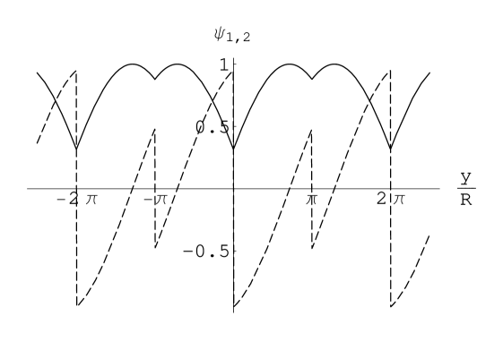
Figure 2.2: The even (continuous) and odd (dashed) components of the zero mode of a fermion field for $\beta=0$, $\delta_{0}=2.5$ and $\delta_{\pi}=1$.

For any $\delta_{\gamma}$ the system is equivalent to a conventional SS compactification with $\beta_{c}=\beta-\delta_{0}-\delta_{\pi}$. We can move to the new continuous eigenfunctions $\Psi_{c}$ performing the following field redefinition:

$$\Psi_{c}(x,y)=e^{\displaystyle{-i\,\alpha(y)\,\widehat{\sigma}_{2}}}\ \Psi(x,y)\leavevmode\nobreak\ .$$ (2.34)

Here the exponential factor removes the discontinuities from $\Psi$ and add a twist $-\delta_{0}-\delta_{\pi}$ to the wave function. Passing from one system to the other we have only performed a local field redefinition. It is a general statement that the physical properties of a quantum mechanical system are invariant under a local field redefinition. We can therefore say that the two systems are really physically equivalent. This is interesting since it suggests that we can move from a description in terms of discontinuous variables to another in terms of smooth fields.

2.1.3 Localized Mass Terms

In the previous section we discussed the equivalence between systems characterized by discontinuous fields and ‘smooth’ systems in which fields are continuous but twisted, showing that a field redefinition exists mapping the mass eigenfunctions of one description into those of the other. Here we would like to further explore the relation between smooth and discontinuous frameworks by showing that the field discontinuities are strictly related to lagrangian terms localized at the fixed points.

We start from the lagrangian ${\cal L}$ of eq. (2.10) for the continuous field $\Psi_{c}$ and we perform the redefinition (2.34). We obtain:

$${\cal L}(\Psi_{c},\partial\Psi_{c}) = {\cal L}(\Psi,\partial\Psi)+{\cal L}_{brane}(\Psi,\partial\Psi)\ \ =$$

$$= i\,\overline{\Psi}\,\bar{\sigma}^{\mu}\,\partial_{\mu}\Psi-\frac{1}{2}\,(\Psi^{T}\,i\widehat{\sigma}^{2}\,\partial_{y}\Psi+h.c.)-\frac{1}{2}\,\bigg{[}\alpha^{\prime}(y)\,\Psi^{T}\Psi+h.c.\bigg{]}$$

with

$$\alpha^{\prime}(y)=\sum_{q=-\infty}^{+\infty}[\delta_{0}\,\delta(y-2q\,\pi R)+\delta_{\pi}\,\delta(y-(2q\,+1)\,\pi R)]\leavevmode\nobreak\ .$$ (2.36)

We observe that jumps are related to mass terms localized at the orbifold fixed points. If we want to explore this relation more deeply we should derive the equation of motion, integrate it around the fixed points and eventually we will recover the discontinuities of fields. But we must pay attention in deriving the equation of motion! Indeed the lagrangian (2.1.3) involves singular terms and the naive use of the variational principle, which is tailored on continuous functions and smooth functionals, would lead to inconsistent results. In order to avoid these problems we regularize $\alpha(y)$ by means of a smooth function $\alpha_{\lambda}(y)$ ($\lambda>0$) which reproduces $\alpha(y)$ in the limit $\lambda\to 0$. Now we can derive the equation of motion which reads:

$$i\widehat{\sigma}^{2}\partial_{y}\Psi=[m-\alpha^{\prime}_{\lambda}(y)]\,\Psi\leavevmode\nobreak\ .$$ (2.37)

Since we are working with regularized functions also $\Psi$ is now continuous, so we can divide eq. (2.37) by $\Psi$. Integrating the result around the fixed points and then taking the limit $\lambda\to 0$ we obtain precisely the jumps of eqs. (2.6)-(2.22). If instead we take this limit directly in eq. (2.37), we immediately see that this equation in the bulk coincides with eq. (2.12), as expected.

To summarize, when going from a smooth to a discontinuous description of the same physical system, singular terms encoding the informations on the discontinuities of fields are generated in the lagrangian. Conversely, when localized terms for bulk fields are present in the 5D lagrangian, as for many phenomenological models currently discussed in the literature, the field variables are affected by discontinuities. These can be derived by analyzing the regularized equation of motion and can be crucial to discuss important physical properties of the system, such as its mass spectrum. In some case we can find a field redefinition that eliminate the discontinuities and provide a smooth description of the system. In section 2.3 we will explain in which cases it is possible to find a field redefinition that completely reabsorbs the localized mass term or, in other terms, which kind of masses can be ascribed to a generalized SS mechanism.

2.2 Generalized Boundary Conditions for Bosons

2.2.1 Boundary Conditions for Bosonic Fields on $S^{1}/\mathbb{Z}_{2}$

In strict analogy with previous sections, we perform here the discussion of the bosonic case, stressing its peculiarities with respect to the fermionic case. As before, we begin by considering a generic 5D theory compactified on the orbifold $S^{1}/\mathbb{Z}_{2}$. We introduce a set of $n$ real 5D bosonic fields $\Phi(x,y)$, which we classify in representations of the 4D Lorentz group. We define the $(T,\mathbb{Z}_{2})$ transformations of the fields by

$$\Phi(y+2\pi R) = U_{\beta}\leavevmode\nobreak\ \Phi(y)$$

$$\Phi(-y) = Z\leavevmode\nobreak\ \Phi(y)\leavevmode\nobreak\ ,$$ (2.38)

where $U_{\beta}$ and $Z$ are constant orthogonal matrices and $Z$ has the property $Z^{2}={\mathbf{1}}$. Also in this case we can choose a basis in which $Z$ is diagonal.

We look for boundary conditions on the fields $\Phi(x,y)$ and their derivatives, in the general class

$$\left(\begin{array}[]{c}\Phi\\ \partial_{y}\Phi\end{array}\right)(\gamma^{+})=V_{\gamma}\leavevmode\nobreak\ \left(\begin{array}[]{c}\Phi\\ \partial_{y}\Phi\end{array}\right)(\gamma^{-})\leavevmode\nobreak\ ,$$ (2.39)

where $V_{\gamma}$ are constant $2n\times 2n$ matrices and $\gamma$ and $\gamma^{\pm}$ are defined in section 2.1.1. We observe that eq. (2.2.1) imply a specific form for the matrix $V_{\beta}$ in (2.39). For the time being we keep a generic expression for $V_{\beta}$, as well as for $V_{0,\pi}$. The reason for which we consider also the derivatives of $\Phi$ will be clear in a while.

We will now constrain the matrices $V_{\gamma}$ by imposing certain consistency requirements on our theory. The spectrum of the theory is determined by the eigenmodes of the differential operator $-\partial^{2}_{y}$, which we require to be self-adjoint with respect to the scalar product defined in eq. (2.3), where now $\Psi$ and $\Phi$ are real scalar fields and $\dagger$ must be converted into $T$. If we consider the matrix element $\langle\Psi|\left(-\partial^{2}_{y}\Phi\right)\rangle$ and we perform a partial integration we obtain:

$$\langle\Psi|\left(-\partial^{2}_{y}\Phi\right)\rangle = \langle\left(-\partial^{2}_{y}\Psi\right)|\Phi\rangle+$$ (2.40)

$$+ \left[\Psi^{T}(y)\partial_{y}\Phi(y)-\partial_{y}\Psi^{T}(y)\Phi(y)\right]^{0^{+}}_{0^{-}}+\leavevmode\nobreak\ \leavevmode\nobreak\ \leavevmode\nobreak\$$

$$+ \left[\Psi^{T}(y)\partial_{y}\Phi(y)-\partial_{y}\Psi^{T}(y)\Phi(y)\right]^{\pi R^{+}}_{\pi R^{-}}+\leavevmode\nobreak\ \leavevmode\nobreak\ \leavevmode\nobreak\$$

$$+ \left[\Psi^{T}(y)\partial_{y}\Phi(y)-\partial_{y}\Psi^{T}(y)\Phi(y)\right]^{y^{-}}_{y^{+}}\leavevmode\nobreak\ ,$$

where $[f(y)]^{a}_{b}=f(a)-f(b)$. Necessary and sufficient conditions for the self-adjointness of the operator $-\partial^{2}_{y}$ are that the three square brackets vanish and the domain of the operator $-\partial^{2}_{y}$ coincide with the domain of its adjoint. In other words, we should impose conditions on $\Phi(y)$ and its first derivative in such a way that the vanishing of the unwanted contributions implies precisely the same conditions on $\Psi(y)$ and its first derivative.

It is easy to show that, in the class of boundary conditions (2.39), this happens when

$$V_{\gamma}J\leavevmode\nobreak\ V_{\gamma}^{T}=J\leavevmode\nobreak\ \leavevmode\nobreak\ \leavevmode\nobreak\ \leavevmode\nobreak\ \leavevmode\nobreak\ \leavevmode\nobreak\ \leavevmode\nobreak\ \leavevmode\nobreak\ \leavevmode\nobreak\ \leavevmode\nobreak\ \leavevmode\nobreak\ \gamma\in(0,\pi,\beta)\leavevmode\nobreak\ ,$$ (2.41)

where $J\equiv i\sigma^{2}$ is the symplectic form in the space $(\Phi,\partial_{y}\Phi)$. Eq. (2.41) restricts $V_{\gamma}$ in the symplectic group $Sp(2n)$. The simplest possibility is offered by $V_{\gamma}={\mathbf{1}}$, for $\gamma=(0,\pi,\beta)$. In this case $U_{\gamma}={\mathbf{1}}$, the fields are periodic and continuous across the orbifold fixed points. When $V_{\beta}\neq{\mathbf{1}}$, the field variables are not periodic and we have a twist. Such boundary conditions are characteristic of the conventional SS mechanism. When $V_{0}$ or $V_{\pi}$ differs from unity, the fields or their derivatives are not continuous across the fixed points and we have jumps. Therefore, in close analogy with the fermionic case, we find that the boundary conditions for bosons allow for both twist and jumps. At variance with the fermionic case, twist and jumps can also affect the first derivative of the field variables. Moreover, the self-adjointness alone does not forbid boundary conditions that mix the fields and their $y$-derivatives. For instance, if we have a single real scalar field $\varphi(y)$, and we parametrize the generic $2\times 2$ matrix $V_{\gamma}$ as:

$$V_{\gamma}=\left(\begin{array}[]{cc}A_{\gamma}&B_{\gamma}\\ C_{\gamma}&D_{\gamma}\end{array}\right)\leavevmode\nobreak\ ,$$ (2.42)

the condition (2.41) reduces to $\det V_{\gamma}=1$, as expected since $Sp(2)$ and $SL(2,R)$ are isomorphic. If $B_{\gamma}$ and $C_{\gamma}$ are not both vanishing, the boundary conditions will mix $\varphi$ and $\partial_{y}\varphi$.

While the field variables and their first derivatives may have twist and jumps, we should require that physical quantities remain periodic and continuous across the orbifold fixed points. This poses a further restriction on the matrices $V_{\gamma}$. If the theory is invariant under global transformations of a group G, we can satisfy this requirement by asking that the matrices $V_{\gamma}$ are in a $2n$-dimensional representation of G. The choice of scalar product made in (2.3) does not allow to consider symmetry transformations of the 5D theory that mix fields and $y$-derivatives. Moreover, it is not restrictive to consider orthogonal representations of G on the space of real fields $\Phi$. In this case, the solution to eq. (2.41) reads

$$V_{\gamma}=\left(\begin{array}[]{cc}U_{\gamma}&0\\ 0&U_{\gamma}\end{array}\right)\leavevmode\nobreak\ \leavevmode\nobreak\ \leavevmode\nobreak\ \leavevmode\nobreak\ \leavevmode\nobreak\ \leavevmode\nobreak\ \leavevmode\nobreak\ \leavevmode\nobreak\ \leavevmode\nobreak\ \leavevmode\nobreak\ \leavevmode\nobreak\ \leavevmode\nobreak\ \leavevmode\nobreak\ \leavevmode\nobreak\ \leavevmode\nobreak\ \leavevmode\nobreak\ U_{\gamma}\in{\rm G}\leavevmode\nobreak\ ,$$ (2.43)

where $U_{\gamma}$ is in an orthogonal $n$-dimensional representation of G.

Finally, we should take into account consistency conditions among the twist, the jumps and the orbifold projection. These are identical to the ones discussed for fermions and are reported here only for completeness:

$$U_{\gamma}\leavevmode\nobreak\ Z\leavevmode\nobreak\ U_{\gamma} = Z\leavevmode\nobreak\ \leavevmode\nobreak\ \leavevmode\nobreak\ \leavevmode\nobreak\ \leavevmode\nobreak\ \leavevmode\nobreak\ \leavevmode\nobreak\ \leavevmode\nobreak\ \leavevmode\nobreak\ \leavevmode\nobreak\ \leavevmode\nobreak\ \leavevmode\nobreak\ \leavevmode\nobreak\ \leavevmode\nobreak\ \leavevmode\nobreak\ \leavevmode\nobreak\ \leavevmode\nobreak\ \gamma\in(0,\pi,\beta)\leavevmode\nobreak\ ,$$

$$\left[U_{0},U_{\beta}\right] = 0\leavevmode\nobreak\ ,$$ (2.44)

$$\left[U_{\pi},U_{\beta}\right] = 0\leavevmode\nobreak\ .$$

Also in this case the parameters of $U_{\gamma}$ can be discrete or continuous, depending on the commutators $[Z,U_{\gamma}]$ and $[U_{0},U_{\pi}]$.

In summary, the allowed boundary conditions on $\Phi(y)$ are specified in eq. (2.39), with the matrices $V_{\gamma}$ satisfying the requirements (2.43)-(2.2.1).

2.2.2 One Scalar Field

It is instructive to analyze in detail the case of a single massless scalar field $\varphi(x,y)$, of definite parity, $Z=+1$ to begin with. We start by writing the equation of motion for $\varphi$

$$-\partial^{2}_{y}\varphi=m^{2}\varphi\leavevmode\nobreak\ ,$$ (2.45)

in each region $y_{q}<y<y_{q+1}$ of the real line, where $y_{q}\equiv q\pi R$ and $q\in{\mathbb{Z}}$. We have defined the mass $m$ through the 4D equation $\partial^{2}\varphi=m^{2}\varphi$. The solutions of these equations can be glued by exploiting the boundary conditions $V_{0}$ and $V_{\pi}$, imposed at $y=y_{2q}$ and $y=y_{2q+1}$, respectively. Finally, the spectrum and the eigenfunctions are obtained by requiring that the solutions have the twist described by $V_{\beta}$.

The equation of motion remains invariant if we multiply $\varphi$ by $\pm 1$, so that the group G of global symmetries is a parity (to be distinguished from the orbifold symmetry $\mathbb{Z}_{2}$ that acts also on the $y$ coordinate). We have $V_{\gamma}=\pm{\mathbf{1}}$. For instance, we are allowed to consider either periodic or anti-periodic fields. We start by analyzing the case of no jumps, $V_{0}=V_{\pi}=+{\mathbf{1}}$. The solutions of the equations of motion, up to an arbitrary $x$-dependent factor, are

$$\varphi_{1}(y)=\cos my\leavevmode\nobreak\ \leavevmode\nobreak\ \leavevmode\nobreak\ \leavevmode\nobreak\ \leavevmode\nobreak\ \leavevmode\nobreak\ \leavevmode\nobreak\ \leavevmode\nobreak\ m\leavevmode\nobreak\ R=\left\{\begin{array}[]{ccc}n&&V_{\beta}=+{\mathbf{1}}\\ n+\displaystyle\frac{1}{2}&&V_{\beta}=-{\mathbf{1}}\end{array}\right.\leavevmode\nobreak\ ,$$ (2.46)

and $n$ is a non-negative integer. It is interesting to compare the result for $V_{\beta}=-{\mathbf{1}}$ with that obtained by assuming a jump in $y=0$: $(V_{0},V_{\pi},V_{\beta})=(-{\mathbf{1}},+{\mathbf{1}},+{\mathbf{1}})$. We find

$$\varphi_{2}(y)=\epsilon(y/2)\leavevmode\nobreak\ \sin my\leavevmode\nobreak\ \leavevmode\nobreak\ \leavevmode\nobreak\ \leavevmode\nobreak\ \leavevmode\nobreak\ \leavevmode\nobreak\ \leavevmode\nobreak\ m\leavevmode\nobreak\ R=n+\frac{1}{2}\leavevmode\nobreak\ .$$ (2.47)

where $\epsilon(y)$ is the sign function on $S^{1}$.

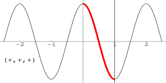
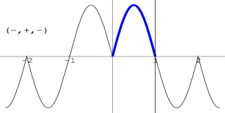
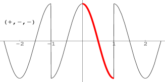
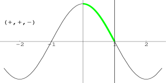
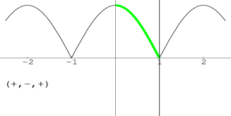
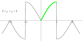
Figure 2.3: Eigenfunctions of $-\partial^{2}_{y}$, for a real even field $\varphi(y)$, versus $y/(\pi R)$. For each boundary condition, labelled by ($V_{0},V_{\pi},V_{\beta}$), the eigenfunction corresponding to the lightest non-vanishing mode is displayed.

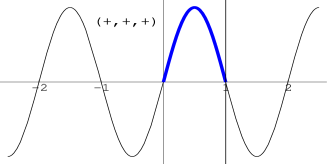
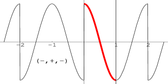
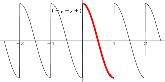
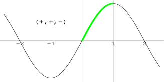
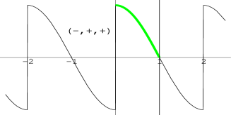
Figure 2.4: Eigenfunctions of $-\partial^{2}_{y}$, for a real odd field $\varphi(y)$, versus $y/(\pi R)$. For each boundary condition, labelled by ($V_{0},V_{\pi},V_{\beta}$), the eigenfunction corresponding to the lightest non-vanishing mode is displayed.

$(V_{0},V_{\pi},V_{\beta})$	$m\leavevmode\nobreak\ R$	eigenfunctions	$\varphi(0)$	$\varphi(\pi R)$
$(+,+,+)$	$n\geq 0$	$\varphi_{1}(y)=\cos my$	$\neq 0$	$\neq 0$
	$n>0$	$\varphi_{5}(y)=\sin my$	$0$	$0$
$(-,+,-)$	$n>0$	$\varphi_{2}(y)=\epsilon(y/2)\leavevmode\nobreak\ \sin my$	$0$	$0$
	$n\geq 0$	$\varphi_{6}(y)=\epsilon(y/2)\leavevmode\nobreak\ \cos my$	${\tt jump}$	$\neq 0$
$(+,-,-)$	$n\geq 0$	$\varphi_{3}(y)=\epsilon(y/2+\pi R/2)\cos my$	$\neq 0$	jump
	$n>0$	$\varphi_{7}(y)=\epsilon(y/2+\pi R/2)\sin my$	$0$	0
$(-,-,+)$	$n>0$	$\varphi_{4}(y)=\epsilon(y)\leavevmode\nobreak\ \sin my$	$0$	$0$
	$n\geq 0$	$\varphi_{8}(y)=\epsilon(y)\leavevmode\nobreak\ \cos my$	jump	jump
$(+,+,-)$	$n+1/2$	$\varphi_{1}(y)=\cos my$	$\neq 0$	$0$
	$n+1/2$	$\varphi_{5}(y)=\sin my$	$0$	$\neq 0$
$(-,+,+)$	$n+1/2$	$\varphi_{2}(y)=\epsilon(y/2)\leavevmode\nobreak\ \sin my$	$0$	$\neq 0$
	$n+1/2$	$\varphi_{6}(y)=\epsilon(y/2)\leavevmode\nobreak\ \cos my$	jump	$0$
$(+,-,+)$	$n+1/2$	$\varphi_{3}(y)=\epsilon(y/2+\pi R/2)\cos my$	$\neq 0$	0
	$n+1/2$	$\varphi_{7}(y)=\epsilon(y/2+\pi R/2)\sin my$	$0$	jump
$(-,-,-)$	$n+1/2$	$\varphi_{4}(y)=\epsilon(y)\leavevmode\nobreak\ \sin my$	$0$	${\tt jump}$
	$n+1/2$	$\varphi_{8}(y)=\epsilon(y)\leavevmode\nobreak\ \cos my$	${\tt jump}$	0

Table 2.1: Eigenvalues and eigenfunctions of $-\partial^{2}_{y}$, for even fields $\varphi_{k}$ $(k=1,2,3,4)$ and odd fields $\varphi_{k}$ $(k=5,6,7,8)$. The spectrum is given in terms of the non-negative integer $n$.

The eigenfunctions (2.46) and (2.47) for $m=1/(2R)$ are compared in the third row of fig. 2.3. We observe that $V_{0}=+{\mathbf{1}}$ implies $\partial_{y}\varphi=0$ at $y=0$, that is Neumann boundary conditions. Instead, if we take $V_{0}=-{\mathbf{1}}$, the even field $\varphi$ should vanish at $y=0$ as for a Dirichelet boundary condition, and this produces a cusp at $y=0$. Despite this difference, the two eigenfunctions are closely related. If compared in the region $0<y<\pi R$, they look the same, up to an exchange between the two walls at $y=0$ and $y=\pi R$. They both vanish at one of the two walls and they have the same non-vanishing value at the other wall, with the same profile in between. Indeed, the two cases are related by a coordinate transformation and a field redefinition:

$$\varphi_{2}(y)=\epsilon(y/2)\leavevmode\nobreak\ \varphi_{1}(y+\pi R)\leavevmode\nobreak\ .$$ (2.48)

If $\varphi_{1}(y)$ is even, continuous and anti-periodic, it is easy to see that the function $\varphi_{2}(y)$ defined in (2.48) is even, periodic and has a cusp in $y=y_{2q}$, where it vanishes. The equations of motion are not affected by the translation $y\to y+\pi R$, which simply exchanges the boundary conditions at $y=y_{2q}$ and $y=y_{2q+1}$. Moreover, the physical properties of a quantum mechanical system are invariant under a local field redefinition. Therefore the two systems related by eq. (2.48) are equivalent.

In table 2.1 we collect spectrum and eigenvalues for all possible cases that are allowed by an even or odd field $\varphi$. We have found it useful to express the solutions in terms of the sign function, which specifies the singularities of the system. Indeed, $\epsilon(y/2)$ is singular in $y=y_{2q}$, $\epsilon(y/2+\pi R/2)$ in $y=y_{2q+1}$ and $\epsilon(y)$ in all $y=y_{q}$. The correct parity of the solutions is guaranteed by the properties of $\epsilon(y)$. Also the periodicity can be easily determined from the fact that $\epsilon(y)$ is periodic, whereas $\epsilon(y/2)$ and $\epsilon(y/2+\pi R/2)$ are anti-periodic.

There are three types of spectra: first, the ordinary KK tower $n/R$ that includes a zero mode; second, an identical spectrum with the absence of the zero mode and, finally, the KK tower shifted by $1/2R$. All systems that possess the same spectrum can be related by field redefinitions that can be easily derived from table 2.1. The only non-trivial transformation, applying only to the case of semi-integer spectrum, is the one in (2.48). For semi-integer spectrum, all $\varphi_{k}$ $(k=1,...8)$ are related. For integer and non-negative spectrum, we have maps among $\varphi_{1}$, $\varphi_{3}$, $\varphi_{6}$ and $\varphi_{8}$. For strictly positive integer spectrum, $\varphi_{2}$, $\varphi_{4}$, $\varphi_{5}$ and $\varphi_{7}$ are related. Thanks to these relations, we can always go from a description in terms of discontinuous field variables to a descriptions by the smooth fields $\varphi_{1}(y)$ or $\varphi_{5}(y)$. Also, as can be seen from figs. 2.3 and 2.4, the behavior in the vicinity of the fixed points is the same for all the eigenfunctions representing the same type of spectrum, up to a possible exchange between the two fixed points. In the presence of a single real field $\varphi$ the parity $Z$ does not seem to have an absolute physical meaning. We find that there are equivalent physical systems with opposite $Z$ parities for $\varphi$.

In conclusion, there are less physically inequivalent systems than independent boundary conditions. There are different boundary conditions that lead to the same spectrum and the corresponding systems are related by field redefinitions. The parameter $V_{0}\cdot V_{\pi}\cdot V_{\beta}$ is equal in equivalent systems. When $V_{0}\cdot V_{\pi}\cdot V_{\beta}=+{\mathbf{1}}$, $mR$ is integer whereas for $V_{0}\cdot V_{\pi}\cdot V_{\beta}=-{\mathbf{1}}$, $mR$ is semi-integer.

2.2.3 More Scalar Fields

Several scalar fields lead to the possibility of exploiting continuous global symmetries to characterize boundary conditions. As an example, we consider here the case of a 5D complex scalar field $\varphi(y)\equiv(\varphi_{1}(y)+i\leavevmode\nobreak\ \varphi_{2}(y))/\sqrt{2}$. Its equation of motion:

$$-\partial^{2}_{y}\varphi=m^{2}\varphi\leavevmode\nobreak\ ,$$ (2.49)

is invariant under global O(2) transformations, acting on $(\varphi_{1},\varphi_{2})$.

We first discuss the case where $Z=diag(+1,-1)$ in the basis $(\varphi_{1},\varphi_{2})$. In this case we can take:

$$U_{\gamma}=\left(\begin{array}[]{cc}\cos\theta_{\gamma}&\sin\theta_{\gamma}\\ -\sin\theta_{\gamma}&\cos\theta_{\gamma}\end{array}\right)\leavevmode\nobreak\ ,$$ (2.50)

which is a symmetry of the theory and satisfies (2.2.1). In general, we can choose three independent angles $\theta_{\gamma}=(\beta,\delta_{0},\delta_{\pi})$ for the twist and the two jumps at $y=0,\pi R$ respectively. The solution of the equation of motion subjected to these boundary conditions can be obtained by the same method used in section 2.2.2. We find:

$$\varphi(y)=e^{\displaystyle i(my-\alpha(y))}\leavevmode\nobreak\ \leavevmode\nobreak\ \leavevmode\nobreak\ ,$$ (2.51)

where

$$m=\frac{n}{R}-\frac{(\beta-\delta_{0}-\delta_{\pi})}{2\pi R}\leavevmode\nobreak\ \leavevmode\nobreak\ \leavevmode\nobreak\ \leavevmode\nobreak\ \leavevmode\nobreak\ \leavevmode\nobreak\ \leavevmode\nobreak\ \leavevmode\nobreak\ \leavevmode\nobreak\ \leavevmode\nobreak\ (n\in{\mathbb{Z}})\leavevmode\nobreak\ ,$$ (2.52)

and $\alpha(y)$ is the function introduced in section 2.1.2. The presence of this function explains why the shift of the spectrum with respect to the KK levels is given by $\beta-\delta_{0}-\delta_{\pi}$ and not by $\beta$ as in the conventional SS mechanism.

When $\beta-\delta_{0}-\delta_{\pi}=0\leavevmode\nobreak\ \leavevmode\nobreak\ \leavevmode\nobreak\ ({\rm mod}\leavevmode\nobreak\ 2\pi)$, the masses are $n/R$ and we can order all massive modes in pairs. Indeed each physical non-vanishing mass $|m|=|n|/R$ $(n\neq 0)$ corresponds to two independent eigenfunctions. For instance, when $\beta=\delta_{0}=\delta_{\pi}=0$, we have $\varphi_{\pm}^{n}=\exp(\pm iny/R)$. This infinite series of degenerate 4D doublets can be interpreted as a consequence of the $O(2)$ symmetry, which is unbroken. A non-vanishing shift of the KK levels induces an explicit breaking of the $O(2)$ symmetry. The order parameter is $\beta-\delta_{0}-\delta_{\pi}$ $({\rm mod}\leavevmode\nobreak\ 2\pi)$. When $\beta-\delta_{0}-\delta_{\pi}$ is non-vanishing (and not a multiple of $2\pi$) the eigenfunctions of the massive modes are no longer paired, each of them corresponding now to a different physical mass. As for the case of a single real field, different boundary conditions may lead to the same spectrum. For instance, it is possible that $O(2)$ remains unbroken, despite the existence of non-trivial boundary conditions, if twist and jumps are such that the combination $\beta-\delta_{0}-\delta_{\pi}$ vanishes mod $2\pi$. Moreover, starting from a generic system with both twist $\beta$ and jumps $\delta_{0,\pi}$ different from zero, we can always move to an equivalent ‘smooth’ theory where the jumps vanish and the twist $\beta^{c}$ of the new scalar field $\varphi^{c}(y)$ is given by $\beta-\delta_{0}-\delta_{\pi}$. The map between the two systems is given by

$$\varphi^{c}(y)=e^{\displaystyle{i\alpha(y)}}\varphi(y)\leavevmode\nobreak\ .$$ (2.53)

The multiplicative factor $e^{\displaystyle{i\alpha(y)}}$ removes the discontinuities from $\varphi(y)$ and add a twist $-\delta_{0}-\delta_{\pi}$ to the wave function.

Another interesting case is that of $Z$ proportional to the identity. If we assign the same $Z$ parity to the real components $\varphi_{1,2}(y)$, then $U_{\gamma}$ commutes with $Z$ and the condition (2.2.1) implies that its eigenvalues are $\pm 1$. If also $[U_{0},U_{\pi}]=0$, then it is not restrictive to go to a field basis where all $U_{\gamma}$ are diagonal, with elements $\pm 1$. This would lead to a discussion qualitatively close to that of section 2.2.2, where twist and jumps were quantized. A new feature occurs if $[U_{0},U_{\pi}]\neq 0$. Consider as an example $Z=U_{\beta}=diag(+1,+1)$ in the basis $(\varphi_{1},\varphi_{2})$. A consistent choice for $U_{0}$ and $U_{\pi}$ is:

$$U_{0}=\left(\begin{array}[]{cc}\cos\delta_{0}&-\sin\delta_{0}\\ -\sin\delta_{0}&-\cos\delta_{0}\end{array}\right)\leavevmode\nobreak\ ,\leavevmode\nobreak\ \leavevmode\nobreak\ \leavevmode\nobreak\ \leavevmode\nobreak\ \leavevmode\nobreak\ \leavevmode\nobreak\ \leavevmode\nobreak\ \leavevmode\nobreak\ \leavevmode\nobreak\ U_{\pi}=\left(\begin{array}[]{cc}1&0\\ 0&-1\end{array}\right)\leavevmode\nobreak\ .$$ (2.54)

Notice that the $O(2)$ matrices $U_{0}$ and $U_{\pi}$ square to 1, as required by the condition (2.2.1). The solutions of the equations of motion are:

$$\phi_{1}(y) = \cos(my-\alpha(y))$$

$$\phi_{2}(y) = \epsilon(y)\sin(my-\alpha(y))\leavevmode\nobreak\ ,$$ (2.55)

where

$$m=\frac{n}{R}+\frac{\delta_{0}}{2\pi R}\leavevmode\nobreak\ \leavevmode\nobreak\ \leavevmode\nobreak\ \leavevmode\nobreak\ \leavevmode\nobreak\ \leavevmode\nobreak\ \leavevmode\nobreak\ \leavevmode\nobreak\ \leavevmode\nobreak\ \leavevmode\nobreak\ (n\in\mathbb{Z})$$ (2.56)

and in $\alpha(y)$ we have to set $\delta_{\pi}=0$. It is interesting to note that this choice of boundary conditions leads to a theory that is physically equivalent to that studied at the beginning of this section, where the fields $\varphi_{1}$ and $\varphi_{2}$ had opposite parity. We can go back to that system and consider the case of periodic fields with a jump at $y=0$: $Z=diag(+1,-1)$, $U_{\pi}=U_{\beta}=1$ and $U_{0}$ as in (2.50) with $\theta_{0}=\delta_{0}$. If we now perform the field redefinition:

$$\varphi_{1}(y)\to\varphi_{1}(y)\leavevmode\nobreak\ ,\leavevmode\nobreak\ \leavevmode\nobreak\ \leavevmode\nobreak\ \leavevmode\nobreak\ \leavevmode\nobreak\ \leavevmode\nobreak\ \leavevmode\nobreak\ \leavevmode\nobreak\ \leavevmode\nobreak\ \leavevmode\nobreak\ \leavevmode\nobreak\ \varphi_{2}(y)\to\epsilon(y)\leavevmode\nobreak\ \varphi_{2}(y)\leavevmode\nobreak\ ,$$ (2.57)

the new field variables are both even and periodic and their jumps are those given in (2.54). It is easy to see that also the solutions (2.51) are mapped into (2.2.3). Moreover, it will be now possible to describe the theory defined by the jumps (2.54) in terms of smooth field variables, characterized by a certain twist.

This correspondence provides another example of equivalent systems, despite a different assignment of the orbifold parity. The presence of discontinuous fields is a generic feature of field theories on orbifolds. The present discussion suggests that at least in some cases these discontinuities may not have any physical significance, being only related to a particular and not compelling choice of field variables.

2.2.4 Brane Action for Bosonic System

In the previous sections we showed the equivalence between bosonic systems characterized by discontinuous fields and ‘smooth’ systems in which fields are continuous but twisted. For each pair of systems characterized by the same mass spectrum we were able to find a local field redefinition, plus a possible discrete translation, mapping the mass eigenfunctions of one system into those of the other system. Here we would like to further explore the relation between smooth and discontinuous systems by showing that the field discontinuities are strictly related to lagrangian terms localized at the fixed points.

We begin by discussing the case of one real scalar field. To fix the ideas we focus on the equivalence between the cases $(+,+,-)$ and $(+,-,+)$ with $Z=1$ of table 2.1. The other cases can be discussed along similar lines. We denote by $\varphi^{c}$ the continuous field $(+,+,-)$ with twist $U_{\beta}=-1$ and by $\varphi$ the periodic field $(+,-,+)$ that has a jump $U_{\pi}=-1$. If we start from the lagrangian $\mathcal{L}$ for the boson $\varphi^{c}$

$$\mathcal{L}(\varphi^{c},\partial\varphi^{c})=-\frac{1}{2}\partial_{M}\varphi^{c}\partial^{M}\varphi^{c}\leavevmode\nobreak\ ,$$ (2.58)

and we perform the field redefinition:

$$\varphi^{c}(y)=\chi(y)\varphi(y)\leavevmode\nobreak\ \leavevmode\nobreak\ \leavevmode\nobreak\ \leavevmode\nobreak\ \leavevmode\nobreak\ \leavevmode\nobreak\ \leavevmode\nobreak\ \leavevmode\nobreak\ \chi(y)\equiv\epsilon(y/2+\pi R/2)\leavevmode\nobreak\ ,$$ (2.59)

we obtain an expression in terms of discontinuous fields and their derivatives, from which it is difficult to derive the correct equation of motion for the system. Indeed the new lagrangian is highly singular and the naive use of the variational principle would lead to inconsistent results. In order to avoid these problems we regularize $\chi(y)$ by means of a smooth function $\chi_{\lambda}(y)$ ($\lambda>0$) which reproduces $\chi(y)$ in the limit $\lambda\to 0$. By performing the substitution:

$$\varphi^{c}(y)=\chi_{\lambda}(y)\leavevmode\nobreak\ \varphi(y)\leavevmode\nobreak\ ,$$ (2.60)

we obtain

$$\mathcal{L}(\varphi^{c},\partial\varphi^{c})=-\frac{1}{2}\chi_{\lambda}^{2}\partial_{M}\varphi\partial^{M}\varphi-\chi_{\lambda}\chi_{\lambda}^{\prime}\varphi\partial_{y}\varphi-\frac{1}{2}\chi_{\lambda}^{\prime 2}\varphi^{2}\leavevmode\nobreak\ .$$ (2.61)

Since the field $\varphi(y)$ is periodic, we can work in the interval $0\leq y\leq 2\pi R$. In the limit $\lambda\to 0$, we find:

$$\mathcal{L}(\varphi^{c},\partial\varphi^{c})=-\frac{1}{2}\chi^{2}\partial_{M}\varphi\partial^{M}\varphi+2\chi\leavevmode\nobreak\ \delta(y-\pi R)\leavevmode\nobreak\ \varphi\partial_{y}\varphi-2\delta^{2}(y-\pi R)\leavevmode\nobreak\ \varphi^{2}\leavevmode\nobreak\ .$$ (2.62)

The action contains quadratic terms for the field $\varphi(y)$ that are localized at $y=\pi R$. However these terms are quite singular and, strictly speaking, are mathematically ill-defined even as distributions. For this reason we derive the equation of motion for $\varphi(y)$ using the regularized action, eq. (2.61), from which we get:

$$\chi_{\lambda}\left(\chi_{\lambda}\partial_{y}^{2}\varphi+2\leavevmode\nobreak\ \chi_{\lambda}^{\prime}\partial_{y}\varphi+\chi_{\lambda}^{\prime\prime}\varphi+\chi_{\lambda}m^{2}\varphi\right)=0\leavevmode\nobreak\ ,$$ (2.63)

where we identified $\partial_{\mu}\partial^{\mu}\varphi$ with $m^{2}\varphi$. The term in brackets should vanish everywhere, since it is continuous and we can choose $\chi_{\lambda}(y)$ different from zero everywhere except at one point between 0 and $2\pi R$. If we finally take the limit $\lambda\to 0$ we obtain the equation of motion for the discontinuous fields:

$$\chi\partial_{y}^{2}\varphi-4\delta(y-\pi R)\partial_{y}\varphi-2\delta^{\prime}(y-\pi R)\varphi+\chi\leavevmode\nobreak\ m^{2}\varphi=0\leavevmode\nobreak\ .$$ (2.64)

Away from the point $y=\pi R$ this equation reduces to the equation of motion for continuous fields: terms with delta functions disappear and we can divide by $\chi(y)$. We obtain:

$$\partial_{y}^{2}\varphi+m^{2}\varphi=0\leavevmode\nobreak\ .$$ (2.65)

Moreover, by integrating eq. (2.64) and its primitive around $y=\pi R$, we find:

$$\begin{array}[]{l}\varphi(\pi R+\xi)=-\varphi(\pi R-\xi)\\ \varphi^{\prime}(\pi R+\xi)=-\varphi^{\prime}(\pi R-\xi)\leavevmode\nobreak\ ,\end{array}$$ (2.66)

which are just the expected jumps.

There is another possibility to derive the correct equation of motion from a singular action, beyond that of adopting a convenient regularization. We illustrate this procedure in the case of one complex scalar field $\varphi(y)$. The basic idea is to use a set of field variables such that their infinitesimal variations, implied by the action principle, are continuous functions of $y$. The action principle requires that the variation of the action $S$, assumed to be a smooth functional of $\varphi$ and $\partial\varphi$, vanishes for infinitesimal variations of the fields from the classical trajectory:

$$\delta S=\int d^{4}x\leavevmode\nobreak\ dy\leavevmode\nobreak\ \frac{\delta\mathcal{L}}{\delta\varphi}\leavevmode\nobreak\ \delta\varphi=0\leavevmode\nobreak\ .$$ (2.67)

If the system is described by discontinuous fields, in general we cannot demonstrate that $\delta\mathcal{L}/\delta\varphi$ vanishes at the singular points, since multiplication/division by discontinuous functions like $\delta\varphi$ is known to produce inequivalent equalities. An exception is the case of fields whose generic variation $\delta\varphi$ is a continuous function, despite the discontinuities of $\varphi$. In this case the action principle leads directly to the usual equation of motion.

We consider as an example the case discussed at the beginning of section 2.2.3. Real and imaginary components of $\varphi$ are respectively even and odd functions of $y$ and we have boundary conditions specified by the matrices $U_{\gamma}$ in eq. (2.50). In particular, the discontinuities of $\varphi_{i}$ $(i=1,2)$ and its $y$-derivative across 0 and $\pi R$ are given by:

$$\left(\begin{array}[]{c}\varphi_{1(2)}\\ \partial_{y}\varphi_{1(2)}\end{array}\right)(\gamma^{+})-\left(\begin{array}[]{c}\varphi_{1(2)}\\ \partial_{y}\varphi_{1(2)}\end{array}\right)(\gamma^{-})=(-)2\tan\frac{\delta_{\gamma}}{2}\left(\begin{array}[]{c}\varphi_{2(1)}\\ \partial_{y}\varphi_{2(1)}\end{array}\right)(\gamma)\leavevmode\nobreak\ ,$$ (2.68)

where $\gamma$ stands for $0$ or $\pi R$, $\gamma^{+(-)}$ denotes $0^{+(-)}$ or $\pi R^{+(-)}$ and

$$\left(\begin{array}[]{c}\varphi_{1(2)}\\ \partial_{y}\varphi_{1(2)}\end{array}\right)(\gamma)\equiv\frac{1}{2}\left[\left(\begin{array}[]{c}\varphi_{1(2)}\\ \partial_{y}\varphi_{1(2)}\end{array}\right)(\gamma^{+})+\left(\begin{array}[]{c}\varphi_{1(2)}\\ \partial_{y}\varphi_{1(2)}\end{array}\right)(\gamma^{-})\right]\leavevmode\nobreak\ .$$ (2.69)

From this we see that a generic variation of $\varphi_{2}$ is discontinuous. The jump of $\delta\varphi_{2}$ across $0$ or $\pi R$ is proportional to the value of $\delta\varphi_{1}$ at that point, which in general is not zero. However we can move to a new set of real fields $\theta$ and $\rho$:

$$\varphi=\rho\leavevmode\nobreak\ e^{i\theta}\leavevmode\nobreak\ ,$$ (2.70)

whose discontinuities from eq. (2.68) read:

$$\left(\begin{array}[]{c}\rho\\ \partial_{y}\rho\end{array}\right)(\gamma^{+})=\left(\begin{array}[]{c}\rho\\ \partial_{y}\rho\end{array}\right)(\gamma^{-})\leavevmode\nobreak\ \leavevmode\nobreak\ \leavevmode\nobreak\ \leavevmode\nobreak\ \leavevmode\nobreak\ \leavevmode\nobreak\ \leavevmode\nobreak\ \leavevmode\nobreak\ \leavevmode\nobreak\ \leavevmode\nobreak\ \left(\begin{array}[]{c}\theta\\ \partial_{y}\theta\end{array}\right)(\gamma^{+})-\left(\begin{array}[]{c}\theta\\ \partial_{y}\theta\end{array}\right)(\gamma^{-})=\left(\begin{array}[]{c}\delta_{\gamma}\\ 0\end{array}\right)\leavevmode\nobreak\ .$$ (2.71)

The discontinuity of $\theta$ at each fixed point is a constant, independent from the value of $\varphi$ at that point. As a consequence, the infinitesimal variation $\delta\theta$ relevant to the action principle is continuous everywhere, including the points $y=0$ and $y=\pi R$. We can derive the action for $(\rho,\theta)$, by starting from the lagrangian expressed in terms of $\varphi^{c}\equiv\rho\exp[i(\theta+\alpha)]$, where the function $\alpha$ has been defined in eq. (2.31):

$$\mathcal{L}(\varphi^{c},\partial\varphi^{c})=-\partial_{M}\varphi^{c{\dagger}}\partial^{M}\varphi^{c}\leavevmode\nobreak\ .$$ (2.72)

In terms of $\rho$ and $\theta$ we have:

$$\mathcal{L}(\rho,\partial\rho,\theta,\partial\theta)=-\partial_{M}\rho\ \partial^{M}\rho-\rho^{2}\partial_{M}(\theta+\alpha)\ \partial^{M}(\theta+\alpha)\leavevmode\nobreak\ .$$ (2.73)

The lagrangian now contains singular terms, localized at the fixed points. The equations of motions, derived from the variational principle, read:

$$\left\{\begin{array}[]{l}\partial_{M}\partial^{M}\rho-\rho\ \partial_{M}(\theta+\alpha)\ \partial^{M}(\theta+\alpha)=0\\ \partial_{M}[\rho^{2}\partial^{M}(\theta+\alpha)]=0\end{array}\right.\leavevmode\nobreak\ .$$ (2.74)

In the bulk $\alpha$ is constant and drops from the previous equations, which then become identical to the equations for the continuous field $\varphi^{c}$, in polar coordinates. Moreover, by integrating eq. (2.74) around the fixed points and by recalling the properties of the function $\alpha$, we reproduce precisely the jumps of eq. (2.71). The same results can be obtained by introducing a regularization for $\alpha$.

To summarize, when going from a smooth to a discontinuous description of the same physical system, singular terms are generated in the lagrangian. In our examples we have quadratic terms localized at the orbifold fixed point which, despite their highly singular behaviour, are necessary for a consistent description of the system. Indeed they encode the discontinuities of the adopted field variables which can be reproduced via the classical equation of motion after appropriate regularization or through a careful application of the standard variational principle. Conversely, when localized terms for bulk fields are present in the 5D lagrangian, as for many phenomenological models currently discussed in the literature, the field variables are affected by discontinuities. These can be derived by analyzing the regularized equation of motion and can be crucial to discuss important physical properties of the system, such as its mass spectrum. In some case we can find a field redefinition that eliminate the discontinuities and provide a smooth description of the system. It would be nice to know precisely when we can perform the redefinition that completely eliminate the localized terms and when they cannot be removed. In the next section we will study this issue.

2.3 Equivalent Effective Lagrangians

In previous sections we showed that different effective lagrangians can describe the same physical system. This is due to the equivalence between the SS twist and the generalized boundary conditions described in detail in sections 2.1.1 and 2.2.1, which are associated to localized mass terms. In this section we find out the class of equivalence of the lagrangians associated to the same spectrum and we classify the conditions the 5D mass terms should satisfy in order to be ascribed to a SS twist. We illustrate this in detail only for fermions; analogous considerations also apply to bosons.

2.3.1 Generation of 5D Mass Terms for Periodic Fields

We consider the lagrangian of eq. (2.10) with twisted periodicity conditions (2.15)-(2.16). The solution to the equation of motion with these boundary conditions is displayed in eqs. (2.17)-(2.19). We now move to a class of equivalent descriptions of this system exploiting the fact that S-matrix elements do not change if we perform a local and non-singular field redefinition. We replace the twisted fields $\Psi(y)$ by periodic ones $\widetilde{\Psi}(y)$:

$$\Psi(y)=V(y)\,\widetilde{\Psi}(y)\,,\;\;\;\;\;\;\;\;\widetilde{\Psi}(y+2\pi R)=\widetilde{\Psi}(y)\,,$$ (2.75)

where $V(y)$ must then be a $2\times 2$ matrix satisfying

$$V(y+2\pi R)=U_{\vec{\beta}}\,V(y)\,,$$ (2.76a)

as can be immediately checked from eqs. (2.15) and (2.75). Besides condition (2.76a), we will impose for our convenience two additional constraints on the matrix $V(y)$. One is

$$V(y)\in SU(2)\,,$$ (2.76b)

which guarantees that the redefinition is non-singular, and that the kinetic terms for $\widetilde{\Psi}(y)$ remain canonical. We also require that the new fields $\widetilde{\psi}_{1}(y)$ and $\widetilde{\psi}_{2}(y)$ have the same parities as the original ones ${\psi}_{1}(y)$ and ${\psi}_{2}(y)$:

$$\left\{\begin{array}[]{rclcc}V_{ij}(-y)&=&+V_{ij}(y)&\phantom{bla}&(ij=11,22)\\ V_{ij}(-y)&=&-V_{ij}(y)&\phantom{bla}&(ij=12,21)\end{array}\right.\,.$$ (2.76c)

Notice that eq. (2.76c) implies $V(0)=\exp\,(\,i\,\theta\,\widehat{\sigma}^{3}\,)$, with $\theta\in{\mathbb{R}}$.

Before exploring the effects of the field redefinition of eq. (2.75), we observe that the solution to the conditions (2.76) is by no means unique. Starting from any given solution $V(y)$, a new set of solutions $V^{\prime}(y)$ can be generated via matrix multiplication:

$$V^{\prime}(y)=W_{L}(y)\,V(y)\,W_{R}(y)\,,$$ (2.77)

provided that the following conditions are satisfied:

$$W_{L}(y+2\pi R)\,U_{\vec{\beta}}=U_{\vec{\beta}}\,W_{L}(y)\,,\;\;\;\;\;W_{R}(y+2\pi R)=W_{R}(y)\,,$$ (2.78a)

$$W_{L,R}(y)\in SU(2)\,,$$ (2.78b)

$$\left\{\begin{array}[]{rclcc}(W_{L,R})_{ij}(-y)&=&+(W_{L,R})_{ij}(y)&\phantom{bla}&(ij=11,22)\\ (W_{L,R})_{ij}(-y)&=&-(W_{L,R})_{ij}(y)&\phantom{bla}&(ij=12,21)\end{array}\right.\,.$$ (2.78c)

We are now ready to explore the effects of the field redefinition of eq. (2.75). The lagrangian ${\cal L}$, expressed in terms of the periodic field $\widetilde{\Psi}(y)$, describes exactly the same physics as before, but its form is now different:

$${\cal L}(\Psi,\partial\Psi) = {\cal L}(\widetilde{\Psi},\partial\widetilde{\Psi})+\left\{-\frac{i}{2}\left[m_{1}(y)+i\,m_{2}(y)\right]\widetilde{\psi}_{1}\widetilde{\psi}_{1}\right.$$ (2.79)

$$+ \left.\frac{i}{2}\left[m_{1}(y)-i\,m_{2}(y)\right]\widetilde{\psi}_{2}\widetilde{\psi}_{2}+i\,m_{3}(y)\,\widetilde{\psi}_{1}\widetilde{\psi}_{2}+{\rm h.c.}\right\}\,,$$

where the mass terms $m_{a}(y)$ $(a=1,2,3)$ are the coefficients of the Maurer-Cartan form

$$m(y)\equiv m_{a}(y)\,\widehat{\sigma}^{a}=-i\,V^{\dagger}(y)\partial_{y}V(y)\,,$$ (2.80)

and satisfy:

$$m_{a}(y+2\pi R)=m_{a}(y)\,,$$ (2.81a)

$$m_{a}(y)\in{\mathbb{R}}\,,$$ (2.81b)

$$m_{1,2}(-y)=+m_{1,2}(y)\,,\;\;\;\;\;m_{3}(-y)=-m_{3}(y)\,,$$ (2.81c)

$$U_{\vec{\beta}}=V(0)\,P\left[\exp\left({\displaystyle i\,\int_{0}^{y}dy^{\prime}m(y^{\prime})}\right)\right]\,P_{<}\left[\exp\left({\displaystyle i\,\int_{y}^{y+2\pi R}dy^{\prime}m(y^{\prime})}\right)\right]\,\times\phantom{blablabla}$$

$$P\,^{\prime}\left[\exp\left({\displaystyle-i\,\int_{0}^{y}dy^{\prime}m(y^{\prime})}\right)\right]V^{\dagger}(0)\,,\;\;\;\;\;\left\{\begin{array}[]{cccc}P=P_{<}&P\,^{\prime}=P_{>}&{\rm for}&y>0\\ P=P_{>}&P\,^{\prime}=P_{<}&{\rm for}&y<0\end{array}\right.\;.$$ (2.81d)

Properties (2.81a)-(2.81c) are in one-to-one correspondence with conditions (2.76a)-(2.76c) on $V(y)$. Eq. (2.81d) is related with eq. (2.76a), and prescribes how the information on the twist of the original fields $\Psi(y)$ is encoded in the new lagrangian. The symbols $P_{<}$ and $P_{>}$ denote inequivalent definitions of path-ordering, specified in appendix B with some useful properties and the proof of eq. (2.81d). Notice that, by taking the trace of both members in eq. (2.81d), we obtain a relation between the Wilson loop and the twist parameter $\beta$:

$$\cos\beta={1\over 2}{\rm tr}\,U_{\vec{\beta}}={1\over 2}{\rm tr}\,P_{<}\left[\exp\left({\displaystyle i\,\int_{y}^{y+2\pi R}dy^{\prime}m(y^{\prime})}\right)\right]\,.$$ (2.82)

Notice also that, because of the freedom of performing global $SU(2)$ transformations with the constant matrix $V(0)$, which are invariances of the lagrangian, different values of the twist $\vec{\beta}$ with the same value of $\beta$ correspond to physically equivalent descriptions.

The mass terms in eq. (2.79) are of three different types, associated with the three possible bilinears $\widetilde{\psi}_{1}\widetilde{\psi}_{1}$, $\widetilde{\psi}_{2}\widetilde{\psi}_{2}$ and $\widetilde{\psi}_{1}\widetilde{\psi}_{2}$. Because of eqs. (2.81), they do not correspond to the most general set of $y$-dependent mass terms allowed by 4D Lorentz invariance, which would be characterized by three independent complex functions. The rôle of the conditions (2.81) is to guarantee the equivalence between the descriptions on the two sides of eq. (2.79).

Also the converse is true. Given a lagrangian such as the one on the right-hand side of eq. (2.79), expressed in terms of periodic fields $\widetilde{\psi}_{i}(y)$ $(i=1,2)$ and with mass terms satisfying eqs. (2.81), we can move to the equivalent lagrangian of eq. (2.10), where all mass terms have been removed and the fields satisfy the periodicity conditions of eq. (2.15), by performing the field redefinition of eq. (2.75). As shown in appendix B, $V(y)$ is given by:

$$V(y)=V(0)\,P\left[\exp\left({\displaystyle i\,\int_{0}^{y}dy^{\prime}m(y^{\prime})}\right)\right]\,,\;\;\;\;\;P=\left\{\begin{array}[]{ccc}P_{<}&{\rm for}&y>0\\ P_{>}&{\rm for}&y<0\end{array}\right.\,.$$ (2.83)

For any $V(0)=\exp\,(\,i\,\theta\,\widehat{\sigma}^{3}\,)$ ($\theta\in{\mathbb{R}}$), conditions (2.76) are satisfied with $U_{\vec{\beta}}$ given by eq. (2.81d). The arbitrariness in $V(0)$ reflects the fact that physically distinct theories are characterized by $\beta$, not by $\vec{\beta}$.

Up to now we have considered only free theories. What happens if we turn on interactions in the lagrangian (2.10)? First of all we ask that the interaction terms are invariant under $SU(2)$. If these terms do not contains $y$-derivatives, they remain unchanged after the redefinition (2.75), so eq. (2.79) still holds true. If instead terms involving $\partial_{y}\Psi$ are present, they will generate, after the field redefinition, additional but controllable contributions to the right hand side of eq. (2.79). Anyway, since the equivalence between two lagrangians related by a local field redefinition holds irrespectively of the explicit form assumed by the interaction terms, the two descriptions of the system will still be equivalent.

2.3.2 Examples and Localization of 5D Mass Terms

From the discussion of the previous section, it is clear that mass ‘profiles’ $m_{a}(y)$ for periodic fields, of the type specified in eq. (2.81), do not have an absolute physical meaning. They can be eliminated from the lagrangian and replaced by a twist, the two descriptions being completely equivalent. Moreover, all lagrangians with the same interaction terms and mass profiles corresponding to the same twist $\vec{\beta}$, as computed from eq. (2.81d), are just different equivalent descriptions of the same physics. Indeed, suppose that ${\cal L}^{1}$ and ${\cal L}^{2}$ are two such lagrangians, and call $V^{I}(y)$ $(I=1,2)$ the local redefinitions mapping ${\cal L}^{I}$ into the lagrangian ${\cal L}$ for the twisted, massless 5D fields $\Psi(y)$. Then ${\cal L}^{1}$ and ${\cal L}^{2}$ are related by the local non-singular field redefinition $V(y)={V^{2}}^{\dagger}(y)V^{1}(y)$. This shows that, in the class of interacting models under consideration, what matters is the twist $\vec{\beta}$ and not the specific form of the mass terms $m_{a}(y)$ enjoying the properties (2.81) . We can make use of this freedom to show that $m_{1,2}(y)$ can be localized at the fixed points $y=0$ and/or $y=\pi R$, without affecting the physical properties of the theory.

As an example, we consider the simple case in which the twist parameter is just

$$\vec{\beta}=(0,\beta,0)\,.$$ (2.84)

Then a frequently used solution to eq. (2.76), for the twist specified by eq. (2.84), is

$$V^{O}(y)=\exp\left(i\,\beta\widehat{\sigma}^{2}\frac{y}{2\pi R}\right)\,,$$ (2.85)

the symbol ‘$O$’ standing for ‘ordinary’. Starting from the lagrangian ${\cal L}$ for the periodic fields $\widetilde{\Psi}(y)$, defined by $V^{O}(y)$ via the redefinition of eq. (2.75), and performing the standard Fourier decomposition of the 5D fields into 4D modes, we can immediately check that the 4D mass eigenvalues and eigenfunctions are indeed given by eqs. (2.17)-(2.19), with $\beta_{1}=0$. Applying eq. (2.80) to $V^{O}(y)$, we find the constant mass profile:

$$m_{1}^{O}(y)=m_{3}^{O}(y)=0\,,\;\;\;\;\;m_{2}^{O}(y)=\frac{\beta}{2\pi R}\,,$$ (2.86)

and we can check that, in agreement with eq. (2.82):

$$\beta=\int_{y}^{y+2\pi R}dy^{\prime}m_{2}^{O}(y^{\prime})\,.$$ (2.87)

We now move to a more general solution of eqs. (2.76) and (2.84), where, in a basis of periodic fields, the system is described by a different lagrangian ${\cal L}^{G}$ (the symbol ‘$G$’ stands for ‘generalized’). ${\cal L}^{G}$ is still of the general form of eq. (2.79), including interaction terms, but now:

$$m_{1}^{G}(y)=m_{3}^{G}(y)=0\,,\;\;\;\;\;m_{2}^{G}(y)\neq 0\,,$$ (2.88)

and $m_{2}^{G}(y)$ is an otherwise arbitrary real, periodic, even function of $y$, with the property that

$$\int_{y}^{y+2\pi R}dy^{\prime}m_{2}^{G}(y^{\prime})=\int_{y}^{y+2\pi R}dy^{\prime}m_{2}^{O}(y^{\prime})=\beta\,.$$ (2.89)

As long as the above properties are satisfied, the two lagrangians ${\cal L}^{O}$ and ${\cal L}^{G}$ are physically equivalent. Two representative and equivalent choices of $m_{2}^{G}(y)$ are illustrated in fig. 2.5:

Figure 2.5: Two representative and equivalent choices for $m_{2}^{G}(y)$, corresponding to $\beta=2$. For reference, the dash-dotted line shows the equivalent constant profile $m_{2}^{O}(y)=1/(\pi R)$.

Figure 2.6: Two representative and equivalent choices for $m_{3}(y)$: the solid line corresponds to $m_{3}(y)=(2\sin y)/R$, the dashed one to $m_{3}(y)=\epsilon(y)/R$.

the dashed line shows a mild (gaussian) localization around the orbifold fixed points, the solid line a strong localization. The interactions between $\widetilde{\Psi}(y)$ and other fields are not determined by the shapes of the fermion eigenmodes and, indirectly, by the profile of $m_{2}(y)$. Neither the mass spectrum, nor the interactions depend on shapes, which are an artifact of the choice of field variables. As long as the twist is kept fixed, shapes can be arbitrarily deformed along $y$, without changing the physics.

A possible special choice for $m_{2}^{G}(y)$ is the singular limit:

$$m_{2}^{G}(y)=\sum_{q=-\infty}^{+\infty}\left[\delta_{0}\,\delta(y-2q\pi R)+\delta_{\pi}\,\delta(y-(2q+1)\pi R)\right]\,,\;\;\;\;\;\delta_{0}+\delta_{\pi}=\beta\,,$$ (2.90)

where what we actually mean is a suitably regularized version of the distribution in eq. (2.90). This description is apparently quite remote from the ‘ordinary’ one. The mass terms vanish everywhere but at the orbifold fixed points, where there are localized contributions to $m_{2}(y)$. The redefinitions bringing from the massive periodic fields of ${\cal L}^{O}$ and ${\cal L}^{G}$ to the corresponding massless twisted 5D fields are:

$$\Psi(y)=V^{O,G}(y)\leavevmode\nobreak\ \widetilde{\Psi}^{O,G}(y)\,,$$ (2.91)

with $V^{O}(y)$ given by eq. (2.85) and

$$V^{G}(y)=\exp\left[i\,\alpha(y)\widehat{\sigma}^{2}\right]\,.$$ (2.92)

Here $\alpha(y)$ is the step function introduced in section 2.1.2. The local field redefinition that relates the two lagrangians ${\cal L}^{O}$ and ${\cal L}^{G}$ is:

$$\widetilde{\Psi}^{G}(y)={V^{G}}^{\dagger}(y)V^{O}(y)\leavevmode\nobreak\ \widetilde{\Psi}^{O}(y)\,.$$ (2.93)

Notice that the periodic fields $\widetilde{\Psi}^{G}(y)$ are not smooth but only piecewise smooth. This can be checked either by integrating the equations of motion for $\widetilde{\Psi}^{G}(y)$, derived from ${\cal L}^{G}$, in a small region around the fixed points, or by making use of the field redefinition in eq. (2.93), recalling that $\widetilde{\Psi}^{O}(y)$ and $V^{O}(y)$ are smooth while $V^{G}(y)$ is not. We find that the fields $\widetilde{\Psi}^{G}(y)$ have cusps and discontinuities described by:

$$\left\{\begin{array}[]{l}\widetilde{\Psi}^{G}(2q\pi R+\xi)=e^{\displaystyle{\,i\,\delta_{0}\sigma^{2}}}\widetilde{\Psi}^{G}(2q\pi R-\xi)\\ \widetilde{\Psi}^{G}[(2q+1)\pi R+\xi]=e^{\displaystyle{\,i\,\delta_{\pi}\sigma^{2}}}\,\widetilde{\Psi}^{G}[(2q+1)\pi R-\xi]\end{array}\right.\,,\;\;\;\;\;(0<\xi\ll 1\,,\,q\in{\mathbb{Z}})\,,$$ (2.94)

where the jumps of the field variables are parametrized by $\delta_{0,\pi}$.

Another simple but instructive example corresponds to a lagrangian for periodic fields of the form in eq. (2.79), where now

$$m_{1}(y)=m_{2}(y)=0\,,\;\;\;\;\;m_{3}(y)\neq 0\,,$$ (2.95)

and $m_{3}(y)$ is an otherwise arbitrary real, odd, periodic function of $y$, as prescribed by eqs. (2.81a)-(2.81c). Notice that, for any such function, eq. (2.82) gives always $\beta=0$, since

$$\int_{y}^{y+2\pi R}dy^{\prime}m_{3}(y^{\prime})=0\,.$$ (2.96)

In other words, real, periodic, odd mass profiles can be completely removed by a field redefinition without introducing a non-trivial twist. Such a field redefinition corresponds to:

$$V(y)=\exp\left[i\int_{0}^{y}dy^{\prime}m_{3}(y^{\prime})\right]\,.$$ (2.97)

Some representative profiles for $m_{3}(y)$ are exhibited in fig. 2.6. Notice that no constant $m_{3}(y)\neq 0$ is allowed by eqs. (2.81a)-(2.81c), and also a $m_{3}(y)\neq 0$ completely localized at $y=2q\pi R$ and/or $y=(2q+1)\pi R$ is forbidden. An allowed possibility is a piecewise constant $m_{3}(y)$, for example:

$$m_{3}(y)=\mu\,\epsilon(y)\,,$$ (2.98)

where $\epsilon(y)$ is the periodic sign function and $\mu$ a real constant with the dimension of a mass.

2.4 Application to Gauge Symmetry Breaking

The generalized boundary conditions discussed in previous sections can be exploited to spontaneously break the gauge invariance of a 5D system. This is well-known as far as the twist is concerned, as described in section 1.2.2. A non-trivial twist induces a shift in the KK levels which lifts the zero modes of the gauge vector bosons: from a 4D point of view the gauge symmetry is thus broken. As we have seen in section 2.2, also the discontinuities of the fields and their first derivatives have a similar effect on the spectrum and we may expect that, in the context of a gauge theory, they lead to spontaneous breaking of the 4D gauge invariance. To analyze these aspects, we focus on a 5D gauge theory defined on our orbifold and based on the gauge group SU(2).

Not all $\mathbb{Z}_{2}$ parity assignments for the gauge fields $A^{a}_{M}(x,y)$ $(a=1,2,3)$, $(M=\mu,5)$ are now possible. The gauge invariance imposes several restrictions. First of all, the action of $\mathbb{Z}_{2}$ on the 4D vector bosons $A^{a}_{\mu}$ should be compatible with the algebra of gauge group. In other words, we should embed $\mathbb{Z}_{2}$ into the automorphism algebra of the gauge group [29]. For SU(2) this leaves two possibilities: either all $A^{a}_{\mu}$ are even, or two of them are odd and one is even. Furthermore, a well-defined parity for the field strength implies that the parity of $A^{a}_{5}$ should be opposite to that of $A^{a}_{\mu}$. In the basis $(A^{1}_{\mu},A^{2}_{\mu},A^{3}_{\mu})$, up to a re-labeling of the three gauge fields, we can consider:

$$({\rm A})\leavevmode\nobreak\ \leavevmode\nobreak\ \leavevmode\nobreak\ \leavevmode\nobreak\ \leavevmode\nobreak\ \leavevmode\nobreak\ \leavevmode\nobreak\ \leavevmode\nobreak\ Z = diag(+1,+1,+1)$$

$$({\rm B})\leavevmode\nobreak\ \leavevmode\nobreak\ \leavevmode\nobreak\ \leavevmode\nobreak\ \leavevmode\nobreak\ \leavevmode\nobreak\ \leavevmode\nobreak\ \leavevmode\nobreak\ Z = diag(-1,-1,+1)\leavevmode\nobreak\ .$$ (2.99)

The boundary conditions on the $A^{a}_{\mu}$ are specified by $3\times 3$ matrices $U_{\gamma}$ that satisfy the consistency relation (2.2.1) and leave the SU(2) algebra invariant. This last requirement can be fulfilled by requiring that $U_{\gamma}$ is an SU(2) global transformation that acts on $(A^{1}_{\mu},A^{2}_{\mu},A^{3}_{\mu})$ in the adjoint representation. Finally, to preserve gauge invariance, the boundary conditions on the scalar fields $A^{a}_{5}$ should be the same as those on the corresponding 4D vector bosons. This can be seen by asking that the various components of the field strength $F^{a}_{MN}$ possess well-defined boundary conditions.

For instance, in the case (A) where all fields $A^{a}_{\mu}$ have even $\mathbb{Z}_{2}$ parity, a consistent assignment is:

$$U_{\beta}=diag(-1,-1,+1)\leavevmode\nobreak\ ,\leavevmode\nobreak\ \leavevmode\nobreak\ \leavevmode\nobreak\ \leavevmode\nobreak\ \leavevmode\nobreak\ \leavevmode\nobreak\ \leavevmode\nobreak\ \leavevmode\nobreak\ U_{0}=U_{\pi}=diag(+1,+1,+1)\leavevmode\nobreak\ .$$ (2.100)

In the gauge $\partial^{M}A^{a}_{M}=0$, the 5D equations of motion read:

$$-\partial^{2}_{y}A^{a}_{M}=m^{2}A^{a}_{M}\leavevmode\nobreak\ .$$ (2.101)

The solutions with the appropriate boundary conditions are:

$$A^{a}_{\mu}(x,y)=A^{a(n_{a})}_{\mu}(x)\cos m_{a}y\leavevmode\nobreak\ \leavevmode\nobreak\ \leavevmode\nobreak\ \leavevmode\nobreak\ \leavevmode\nobreak\ \leavevmode\nobreak\ \leavevmode\nobreak\ \leavevmode\nobreak\ m_{1,2}R=n_{1,2}+\frac{1}{2}\leavevmode\nobreak\ \leavevmode\nobreak\ \leavevmode\nobreak\ \leavevmode\nobreak\ \leavevmode\nobreak\ \leavevmode\nobreak\ \leavevmode\nobreak\ \leavevmode\nobreak\ m_{3}R=n_{3}\leavevmode\nobreak\ ,$$ (2.102)

where $n_{1,2,3}$ are non-negative integers. The only zero mode of the system is $A^{3(0)}_{\mu}(x)$ and, from a 4D point of view the original gauge symmetry is broken down to the U(1) associated to this massless gauge vector boson. The breaking of the 5D SU(2) gauge symmetry is spontaneous and each mode in (2.102), but $A^{3(0)}_{\mu}(x)$, becomes massive via a Higgs mechanism. The unphysical Goldstone bosons are the modes of the fields $A^{a}_{5}(x,y)$, which are all absorbed by the corresponding massive vector bosons. On the wall at $y=0$ all the gauge fields and the parameters of the gauge transformations are non-vanishing. Here all the constraints coming from the full 5D gauge invariance are effective. On the contrary on the wall at $y=\pi R$, only $A^{3}_{\mu}(x,y)$ and the corresponding gauge parameter are different from zero. Therefore the effective symmetry at the fixed point $y=\pi R$ is the U(1) related to the 4D gauge boson $A^{3}_{\mu}(x,\pi R)$. This kind of setup where the gauge symmetry is broken by twisted orbifold boundary conditions and the two fixed points are characterized by two different effective 4D symmetries has recently received lot of attention, for its successful application in the context of GUTs (see sections 1.2.2).

We have just shown how a gauge symmetry can be broken by means of twisted fields. It is interesting to note that the same physical system can be described by using periodic field variables, with discontinuities at the fixed points. This is achieved, for instance, by means of the boundary conditions

$$U_{\beta}=U_{0}=diag(+1,+1,+1)\leavevmode\nobreak\ ,\leavevmode\nobreak\ \leavevmode\nobreak\ \leavevmode\nobreak\ \leavevmode\nobreak\ \leavevmode\nobreak\ \leavevmode\nobreak\ \leavevmode\nobreak\ \leavevmode\nobreak\ U_{\pi}=diag(-1,-1,+1)\leavevmode\nobreak\ .$$ (2.103)

The solutions to the equations of motion (2.101) are:

$$A^{a}_{\mu}(x,y) = A^{a(n_{a})}_{\mu}(x)\leavevmode\nobreak\ \epsilon(y/2+\pi R/2)\cos m_{a}y\leavevmode\nobreak\ \leavevmode\nobreak\ \leavevmode\nobreak\ \leavevmode\nobreak\ \leavevmode\nobreak\ \leavevmode\nobreak\ m_{a}R=n_{a}+\frac{1}{2}\leavevmode\nobreak\ \leavevmode\nobreak\ \leavevmode\nobreak\ \leavevmode\nobreak\ \leavevmode\nobreak\ \leavevmode\nobreak\ \leavevmode\nobreak\ \leavevmode\nobreak\ (a=1,2)$$

$$A^{3}_{\mu}(x,y) = A^{3(n_{3})}_{\mu}(x)\cos m_{3}y\leavevmode\nobreak\ \leavevmode\nobreak\ \leavevmode\nobreak\ \leavevmode\nobreak\ \leavevmode\nobreak\ \leavevmode\nobreak\ \leavevmode\nobreak\ \leavevmode\nobreak\ \leavevmode\nobreak\ \leavevmode\nobreak\ \leavevmode\nobreak\ \leavevmode\nobreak\ \leavevmode\nobreak\ \leavevmode\nobreak\ \leavevmode\nobreak\ \leavevmode\nobreak\ \leavevmode\nobreak\ \leavevmode\nobreak\ \leavevmode\nobreak\ \leavevmode\nobreak\ \leavevmode\nobreak\ \leavevmode\nobreak\ \leavevmode\nobreak\ \leavevmode\nobreak\ \leavevmode\nobreak\ \leavevmode\nobreak\ m_{3}R=n_{3}\leavevmode\nobreak\ ,$$ (2.104)

where $n_{1,2,3}$ are non-negative integers. The new solutions $A^{1,2}_{\mu}$ have cusps at $y=\pi R$ (mod $2\pi$), as the profiles denoted by $(+,-,+)$ in fig. 2.3. The two descriptions are related by the field redefinition

$$A^{a}_{\mu}(x,y)\leavevmode\nobreak\ \to\leavevmode\nobreak\ \epsilon(y/2+\pi R/2)\leavevmode\nobreak\ A^{a}_{\mu}(x,y)\leavevmode\nobreak\ \leavevmode\nobreak\ \leavevmode\nobreak\ \leavevmode\nobreak\ \leavevmode\nobreak\ \leavevmode\nobreak\ \leavevmode\nobreak\ \leavevmode\nobreak\ (a=1,2)$$ (2.105)

which is a local transformation. As already stressed, this assures that the description in terms of smooth twisted fields is physically equivalent to the one with periodic and discontinuous fields.

In the previous example the boundary conditions $U_{\gamma}$ commute among themselves and with the parity $Z$. As a consequence the rank of the gauge group SU(2) is conserved in the symmetry breaking. We can lower the rank by assuming $[U_{\gamma},Z]\neq 0$. As an example, we consider the parity (B) of eq. (2.4) and boundary conditions described by:

$$U_{\gamma}=e^{\displaystyle\theta_{\gamma}T^{2}}\leavevmode\nobreak\ \leavevmode\nobreak\ \leavevmode\nobreak\ \leavevmode\nobreak\ \leavevmode\nobreak\ \leavevmode\nobreak\ \leavevmode\nobreak\ \leavevmode\nobreak\ T^{2}=\left(\begin{array}[]{ccc}0&0&1\\ 0&0&0\\ -1&0&0\end{array}\right)\leavevmode\nobreak\ ,$$ (2.106)

in the basis $(A^{1}_{\mu},A^{2}_{\mu},A^{3}_{\mu})$. We allow, at the same time, for a twist $\theta_{\beta}\equiv\beta$ and two jumps $\theta_{0(\pi)}\equiv\delta_{0}(\delta_{\pi})$. The matrices $U_{\gamma}$ are block diagonal and do not mix the index 2 with the indices (1,3). Thus the boundary conditions are trivial for the odd field $A^{2}_{\mu}$ and its derivative. Non-trivial boundary conditions involve the fields $A^{1}_{\mu}$ and $A^{3}_{\mu}$. By solving the equations (2.101), we obtain:

$$A^{1}_{\mu}(x,y) = A^{(n)}_{\mu}(x)\leavevmode\nobreak\ \sin(my-\alpha(y))$$

$$A^{2}_{\mu}(x,y) = A^{2(n_{2})}_{\mu}(x)\leavevmode\nobreak\ \sin m_{2}y\leavevmode\nobreak\ \leavevmode\nobreak\ \leavevmode\nobreak\ \leavevmode\nobreak\ \leavevmode\nobreak\ \leavevmode\nobreak\ \leavevmode\nobreak\ \leavevmode\nobreak\ \leavevmode\nobreak\ \leavevmode\nobreak\ \leavevmode\nobreak\ \leavevmode\nobreak\ \leavevmode\nobreak\ \leavevmode\nobreak\ \leavevmode\nobreak\ \leavevmode\nobreak\ \leavevmode\nobreak\ \leavevmode\nobreak\ m_{2}R=n_{2}$$ (2.107)

$$A^{3}_{\mu}(x,y) = A^{(n)}_{\mu}(x)\leavevmode\nobreak\ \cos(my-\alpha(y))\leavevmode\nobreak\ \leavevmode\nobreak\ \leavevmode\nobreak\ \leavevmode\nobreak\ \leavevmode\nobreak\ \leavevmode\nobreak\ \leavevmode\nobreak\ \leavevmode\nobreak\ \leavevmode\nobreak\ mR=n-\frac{\beta-\delta_{0}-\delta_{\pi}}{2\pi}\leavevmode\nobreak\ ,$$

where $n\in\mathbb{Z}$, $n_{2}$ is a positive integer and the function $\alpha(y)$ has been defined in section 2.1.2. If $\beta-\delta_{0}-\delta_{\pi}=0$ (mod $2\pi$), we have a zero mode $A^{(0)}_{\mu}(x)$ and the gauge symmetry is spontaneously broken down to U(1), as in the previously discussed examples. When $\beta-\delta_{0}-\delta_{\pi}\neq 0$ (mod $2\pi$), there are no zero modes and SU(2) is completely broken. We can go continuously from this phase to the phase where a U(1) survives, by changing the twist and/or the jump parameters. We may thus have a situation where U(1) is broken by a very small amount, compared to the scale $1/R$ that characterizes the SU(2) breaking. The U(1) breaking order parameter is the combination $\beta-\delta_{0}-\delta_{\pi}$. The same physical system is described by a double infinity of boundary conditions, those that reproduce the same order parameter. All these descriptions are equivalent and are related by field redefinitions. In the class of all equivalent theories one of them is described by continuous fields $A^{a\,c}_{\mu}(x,y)$. We go from the generic theory described in terms of $(\beta,\delta_{0},\delta_{\pi})$ to that characterized by $(\beta^{c}\equiv\beta-\delta_{0}-\delta_{\pi},\delta^{c}_{0}\equiv 0,\delta^{c}_{\pi}\equiv 0)$, via the field transformation:

$$\left(\begin{array}[]{c}A^{1\,c}_{\mu}\\ A^{3\,c}_{\mu}\end{array}\right)=\left(\begin{array}[]{cc}\cos\alpha(y)&-\sin\alpha(y)\\ \sin\alpha(y)&\cos\alpha(y)\\ \end{array}\right)\left(\begin{array}[]{c}A^{1}_{\mu}\\ A^{3}_{\mu}\end{array}\right)\leavevmode\nobreak\ .$$ (2.108)

In section 2.2.4 we learned that discontinuous fields are associated to localized lagrangian terms. We would like to derive these terms also in this case with gauge fields. The main difference with respect to the free theory examples discussed in section 2.2.4 is that now the lagrangian contains derivative interactions among the gauge bosons. In principle these could lead to localized interaction terms, that would provide a non-trivial extension of the framework considered up to now. To investigate this point we start from the 5D SU(2) Yang-Mills theory defined by the parity (A) of eq. (2.4) and by the boundary conditions of eq. (2.100). No jumps are present and the overall lagrangian is given only by the ‘bulk’ term:

$$\mathcal{L}=-\frac{1}{4}F^{a\,c}_{MN}F^{a\,c\,MN}\leavevmode\nobreak\ .$$ (2.109)

It is particularly convenient to discuss the physics in the unitary gauge, where all the would-be Goldstone bosons, eaten up by the massive KK modes, vanish:

$$A_{5}^{a\,c}(x,y)\equiv 0\leavevmode\nobreak\ \leavevmode\nobreak\ \leavevmode\nobreak\ \leavevmode\nobreak\ \leavevmode\nobreak\ \leavevmode\nobreak\ \leavevmode\nobreak\ (a=1,2,3)\leavevmode\nobreak\ .$$ (2.110)

In this gauge $F^{a\,c}_{5\mu}\equiv\partial_{y}A^{a\,c}_{\mu}$ and the lagrangian (2.109) reads:

$$\mathcal{L}=-\frac{1}{4}F^{a\,c}_{\mu\nu}F^{a\,c\,\mu\nu}-\frac{1}{2}\partial_{y}A^{a\,c}_{\mu}\partial_{y}A^{a\,c\,\mu}\leavevmode\nobreak\ .$$ (2.111)

To discuss the case of discontinuous gauge vector bosons, such as those associated to boundary conditions (2.103), we can simply perform the field redefinition:

$$A^{\hat{a}}_{M}(x,y)\leavevmode\nobreak\ =\leavevmode\nobreak\ \chi_{\lambda}(y)\leavevmode\nobreak\ A^{\hat{a}c}_{M}(x,y)\leavevmode\nobreak\ \leavevmode\nobreak\ \leavevmode\nobreak\ \leavevmode\nobreak\ \leavevmode\nobreak\ \leavevmode\nobreak\ \leavevmode\nobreak\ \leavevmode\nobreak\ ({\hat{a}}=1,2)\leavevmode\nobreak\ ,$$ (2.112)

where the function $\chi_{\lambda}(y)$ represents a regularized version of $\epsilon(y/2+\pi R/2)$. Such redefinition maps the twisted, smooth fields obeying (2.100) into periodic variables, discontinuous at $y=\pi R$, as specified in (2.103). Notice that this redefinition does not change the gauge condition (2.110). If we plug the transformation (2.112) into the lagrangian (2.111), we obtain the lagrangian for the system characterized by discontinuous fields. We stress that, since this field redefinition is local, the physics remains the same: the two systems are completely equivalent. The S-matrix elements computed with the two lagrangians are identical and, of course, this equivalence includes the non-trivial non-abelian interactions. Our aim here is only to understand how the physics, in particular the non-abelian interactions, are described by the new, discontinuous variables. From eq. (2.111) we can already conclude that no localized non-abelian interaction terms arise from the field redefinition (2.112), in the unitary gauge. Indeed, the only term containing a $y$ derivative is quadratic, and, after the substitution (2.112), we will obtain terms analogous to those discussed in (2.61) for the case of a single scalar field. We find:

$$\mathcal{L} = -\frac{1}{4}\tilde{F}^{3}_{\mu\nu}\tilde{F}^{3\mu\nu}-\frac{1}{2}\partial_{y}A^{3}_{\mu}\partial_{y}A^{3\mu}+$$ (2.113)

$$+ \frac{1}{2}\chi_{\lambda}^{2}f^{3\hat{b}\hat{c}}A^{\hat{b}}_{\mu}A^{\hat{c}}_{\nu}\tilde{F}^{3\mu\nu}-\frac{1}{4}\chi_{\lambda}^{4}f^{3\hat{b}\hat{c}}f^{3\hat{d}\hat{e}}A^{\hat{b}}_{\mu}A^{\hat{c}}_{\nu}A^{\hat{d}\mu}A^{\hat{e}\nu}-$$

$$- \frac{1}{4}\chi_{\lambda}^{2}F^{\hat{a}}_{\mu\nu}F^{\hat{a}\mu\nu}-\frac{1}{2}\chi_{\lambda}^{2}\partial_{y}A^{\hat{a}}_{\mu}\partial_{y}A^{{\hat{a}}\mu}-$$

$$- \frac{1}{2}\leavevmode\nobreak\ \chi_{\lambda}^{\prime 2}\leavevmode\nobreak\ A^{\hat{a}}_{\mu}A^{\hat{a}\mu}-\chi_{\lambda}\chi_{\lambda}^{\prime}\leavevmode\nobreak\ A^{\hat{a}\mu}\leavevmode\nobreak\ \partial_{5}A^{\hat{a}}_{\mu}\leavevmode\nobreak\ ,$$

where $\tilde{F}^{3}_{\mu\nu}=\partial_{\mu}A^{3}_{\nu}-\partial_{\nu}A^{3}_{\mu}$, $f^{abc}$ are the structure constants of SU(2) and the indices $\hat{a},\hat{b},...$ run over 1,2. In the limit $\lambda\to 0$, the non-abelian interactions are formally unchanged, whereas the last line represents a set of localized quadratic terms. As discussed in the case of a real scalar field, such terms guarantee, via the equations of motion, that the fields obey the new boundary conditions (2.103). In a general gauge, interaction terms localized at $y=\pi R$ are present, but they involve non-physical would-be Goldstone bosons.

Fields	$(Z,U_{\beta})$	$\psi_{K}(y)$	$(Z,U_{\pi})$	$\psi_{our}(y)$	$m$
$A^{a}_{\mu},\lambda_{L}^{2a},H^{D}_{u},H^{D}_{d}$	$(+,+)$	$cos(my)$	$(+,+)$	$cos(my)$	$\frac{2n}{R}$
$A^{\hat{a}}_{\mu},\lambda_{L}^{2\hat{a}},H^{T}_{u},H^{T}_{d}$	$(+,-)$	$cos(my)$	$(+,-)$	$\epsilon(\frac{y}{2}+\frac{\pi R}{2})cos(my)$	$\frac{2n+1}{R}$
$A^{\hat{a}}_{5},\Sigma^{\hat{a}},\lambda_{L}^{1\hat{a}},\widehat{H}^{T}_{u},\widehat{H}^{T}_{d}$	$(-,-)$	$sin(my)$	$(-,-)$	$\epsilon(\frac{y}{2}+\frac{\pi R}{2})sin(my)$	$\frac{2n+1}{R}$
$A^{a}_{5},\Sigma^{a},\lambda_{L}^{1a},\widehat{H}^{D}_{u},\widehat{H}^{D}_{d}$	$(-,+)$	$sin(my)$	$(-,+)$	$sin(my)$	$\frac{2n+2}{R}$

Table 2.2: Boundary conditions, eigenfunctions and spectra for fields in the Kawamura model in the traditional scheme ($2^{nd}$, $3^{rd}$ and $6^{th}$ columns) and in our framework ($4^{th}$, $5^{th}$ and $6^{th}$ columns).

After having studied the case of $SU(2)$, we now briefly apply our considerations to a realistic model. We consider the GUT proposed by Kawamura in ref. [19] and described in section 1.2.2 and we re-interpret this model with generalized boundary conditions. We choose parity assignments identical to the original ones, but, instead of a twist, we require that some fields jump in $y=\pi R$. Among gauge fields only the vector bosons of the coset $SU(5)\leavevmode\nobreak\ /\leavevmode\nobreak\ SU(3)\times SU(2)\times U(1)$ jump. In table 2.2 boundary conditions, eigenfunctions and eigenvalues for both the original model and for our framework are shown. We can observe that the spectra are the same for all fields in both cases, while eigenfunctions are identical for continuous fields but different for jumping fields. The relation between the two sets of eigenfunctions is analogous to the one between eq. (2.102) and eq. (2.4) and they are related by a local field redefinition analogous to eq. (2.105).

Also in this case we can perform the field redefinition at the level of the lagrangian in order to find the localized terms related to jumps in this model. For simplicity we consider only the Yang-Mills term of the lagrangian, neglecting both the supersymmetric part and the Higgs terms:

$$\mathcal{L}=-\frac{1}{4}F^{\alpha}_{MN}F^{\alpha MN}\leavevmode\nobreak\ .$$ (2.114)

Applying the usual field redefinition and choosing the unitary gauge, this becomes:

$$\mathcal{L} = -\frac{1}{4}\tilde{F}^{a}_{\mu\nu}\tilde{F}^{a\mu\nu}-\frac{1}{2}\partial_{y}A^{a}_{\mu}\partial_{y}A^{a\mu}+$$ (2.115)

$$+ \frac{1}{2}\epsilon^{2}f^{a\hat{b}\hat{c}}A^{\hat{b}}_{\mu}A^{\hat{c}}_{\nu}\tilde{F}^{a\mu\nu}-\frac{1}{4}\epsilon^{4}f^{a\hat{b}\hat{c}}f^{a\hat{d}\hat{e}}A^{\hat{b}}_{\mu}A^{\hat{c}}_{\nu}A^{\hat{d}\mu}A^{\hat{e}\nu}-$$

$$- \frac{1}{4}\epsilon^{2}F^{\hat{a}}_{\mu\nu}F^{\hat{a}\mu\nu}-\frac{1}{2}\epsilon^{2}\partial_{y}A^{\hat{a}}_{\mu}\partial_{y}A^{{\hat{a}}\mu}-$$

$$- 2\leavevmode\nobreak\ \delta^{2}(y-\pi R)\leavevmode\nobreak\ A^{\hat{a}}_{\mu}A^{\hat{a}\mu}+2\epsilon\delta(y-\pi R)\leavevmode\nobreak\ A^{\hat{a}\mu}\leavevmode\nobreak\ \partial_{5}A^{\hat{a}}_{\mu}\leavevmode\nobreak\ ,$$

where $\tilde{F}^{a}_{\mu\nu}=\partial_{\mu}A^{a}_{\nu}-\partial_{\nu}A^{a}_{\mu}-f^{abc}A^{b}_{\mu}A^{c}_{\nu}$. Also in this example we obtain mass terms that are localized where the fields have discontinuities.

2.5 Application to Supersymmetry Breaking

In this section we exploit the demonstrated equivalence between “twist and jumps” to show how brane-induced SUSY breaking in 5D, which reproduces the main features of gaugino condensation in M-theory, is equivalent to SS SUSY breaking.

We consider pure 5D Poincaré supergravity in its on-shell formulation [30]. The supergravity multiplet contains the fünfbein $e_{M}^{\;A}$, the gravitino $\Psi_{M}$ and the graviphoton $B_{M}$. The 5D bulk Lagrangian is:

$$\kappa{\cal L}_{bulk} = -{1\over 2\kappa^{2}}e_{5}R_{5}-{1\over 4}e_{5}F_{MN}F^{MN}-{\kappa\over 6\sqrt{6}}\epsilon^{MNOPQ}F_{MN}F_{OP}B_{Q}+$$ (2.116)

$$+i\epsilon^{MNOPQ}\overline{\Psi}_{M}\Sigma_{NO}D_{P}\Psi_{Q}-i\sqrt{3\over 2}{\kappa\over 2}e_{5}F_{MN}\overline{\Psi}^{M}\Psi^{N}+$$

$$+i\sqrt{3\over 2}{\kappa\over 4}\epsilon^{MNOPQ}F_{MN}\overline{\Psi}_{O}\Gamma_{P}\Psi_{Q}+{\rm 4\!\!-\!\!fermion\leavevmode\nobreak\ terms}\leavevmode\nobreak\ .$$

Here $\kappa=M_{5}^{-1}=(\pi R/M_{Pl}^{2})^{\frac{1}{3}}$ is the inverse reduced 5D Planck mass ($R$ is the compactification radius), $R_{5}$ is the 5D scalar curvature, $e_{5}=\det e_{M}^{\;A}$, $e_{4}=\det e_{m}^{\;a}$ (where the latter are the components of the fünfbein with 4D indices), $\epsilon^{MNOPQ}=e_{5}e_{A}^{\;M}e_{B}^{\;N}e_{C}^{\;O}e_{D}^{\;P}e_{E}^{\;Q}\epsilon^{ABCDE}$, $\epsilon^{mnop}=e_{4}e_{a}^{\;m}e_{b}^{\;n}e_{c}^{\;o}e_{d}^{\;p}\epsilon^{abcd}$ and $\epsilon^{\hat{0}\hat{1}\hat{2}\hat{3}\hat{5}}=\epsilon^{\hat{0}\hat{1}\hat{2}\hat{3}}=+1$. This lagrangian is invariant under appropriate SUSY transformations (see eq. (2.2) of ref. [28]).

We work on the orbifold $S^{1}/\mathbb{Z}_{2}$ and we assume that our fields are fluctuations of the background

$$\langle g_{MN}\rangle=\left(\begin{array}[]{cc}\eta_{mn}&0\\ 0&r^{2}\end{array}\right)\leavevmode\nobreak\ ,$$ (2.117)

where $r^{2}=(RM_{5})^{2}=(M_{Pl}^{2}R^{2}/\pi)^{2/3}$ and all other background fields are assumed to vanish. We define the action of the orbifold symmetry in such a way that the action, the transformation laws and the background are all invariant. Writing the spinors in the notation (A) of eq. (2.7), we assign even $\mathbb{Z}_{2}$-parity to

$$e_{m}^{\;a}\leavevmode\nobreak\ \leavevmode\nobreak\ \leavevmode\nobreak\ \leavevmode\nobreak\ \leavevmode\nobreak\ e_{5\hat{5}}\leavevmode\nobreak\ \leavevmode\nobreak\ \leavevmode\nobreak\ \leavevmode\nobreak\ \leavevmode\nobreak\ B_{5}\leavevmode\nobreak\ \leavevmode\nobreak\ \leavevmode\nobreak\ \leavevmode\nobreak\ \leavevmode\nobreak\ \psi_{m}^{1}\leavevmode\nobreak\ \leavevmode\nobreak\ \leavevmode\nobreak\ \leavevmode\nobreak\ \leavevmode\nobreak\ \psi_{5}^{2}\leavevmode\nobreak\ \leavevmode\nobreak\ \leavevmode\nobreak\ \leavevmode\nobreak\ \leavevmode\nobreak\ \eta^{1}\leavevmode\nobreak\ ,$$ (2.118)

and odd $\mathbb{Z}_{2}$-parity to

$$e_{5}^{\;a}\leavevmode\nobreak\ \leavevmode\nobreak\ \leavevmode\nobreak\ \leavevmode\nobreak\ \leavevmode\nobreak\ e_{m\hat{5}}\leavevmode\nobreak\ \leavevmode\nobreak\ \leavevmode\nobreak\ \leavevmode\nobreak\ \leavevmode\nobreak\ B_{m}\leavevmode\nobreak\ \leavevmode\nobreak\ \leavevmode\nobreak\ \leavevmode\nobreak\ \leavevmode\nobreak\ \psi_{m}^{2}\leavevmode\nobreak\ \leavevmode\nobreak\ \leavevmode\nobreak\ \leavevmode\nobreak\ \leavevmode\nobreak\ \psi_{5}^{1}\leavevmode\nobreak\ \leavevmode\nobreak\ \leavevmode\nobreak\ \leavevmode\nobreak\ \leavevmode\nobreak\ \eta^{2}\leavevmode\nobreak\ .$$ (2.119)

From a 4D point of view, the physical spectrum contains one massless $N=1$ gravitational multiplet, with spins $(2,3/2)$, built from the zero modes of $e_{m}^{\;a}$ and $\psi_{m}^{1}$; one massless $N=1$ chiral multiplet, with spins $(1/2,0)$, composed of the zero modes of $\psi_{5}^{2}$, $e_{5\hat{5}}$ and $B_{5}$; and an infinite series of massive multiplets of $N=2$ supergravity, with spins $(2,3/2,3/2,1)$ and squared masses

$$M_{n}^{2}={n^{2}\over R^{2}}\leavevmode\nobreak\ ,\leavevmode\nobreak\ \leavevmode\nobreak\ \leavevmode\nobreak\ \leavevmode\nobreak\ \leavevmode\nobreak\ (n=1,2,\ldots)\leavevmode\nobreak\ .$$ (2.120)

The KK tower gains mass through an infinite series of Higgs and super-Higgs effects, each occurring at its own mass level. The KK gravitons and graviphotons gain mass by eating the Fourier modes of the fields $g_{m5}$, $g_{55}$ and $B_{5}$, while the massive gravitinos eat the Fourier modes of the field $\Psi_{5}$. This is consistent with the fact that the parameter of 5D SUSY, $\eta(x^{M})$, has an infinite number of Fourier modes. Each of the modes generates a SUSY; in the absence of matter, all but one are spontaneously broken. The broken SUSYs implement an infinite series of super-Higgs effects for the massive gravitinos. The remaining SUSY is the $N=1$ of the 4D low-energy effective action.

We now introduce the brane action. Since we are not interested in the brane dynamics, we imagine that the brane fields are integrated out, leaving a constant superpotential vev on each brane. The action is:

$$S_{brane}={\kappa^{2}\over 2}\,\int d^{4}x\int_{-\pi\kappa}^{+\pi\kappa}dy\;e_{4}\left[\delta(y)\overline{P_{0}}+\delta(y-\pi\kappa)\overline{P_{\pi}}\right]\,\psi_{a}^{1}\sigma^{ab}\psi_{b}^{1}+{\rm\;h.c.}\leavevmode\nobreak\ ,$$ (2.121)

where $P_{0}$ and $P_{\pi}$ are complex constants with the dimension of $(mass)^{3}$ which parametrize the vevs of the superpotentials. With a simple modification of the bulk SUSY transformations the whole action $S_{bulk}+S_{brane}$ is invariant (for details see ref. [28]).

The presence of these superpotential vevs induces SUSY breaking. In section 4 of ref. [28] the symmetry breaking mechanism as well as the super-Higgs effect are studied in details. Here we report only the fundamental results. When $\overline{P_{0}}\neq-\overline{P_{\pi}}$ SUSY is broken spontaneously: the fields $\psi^{1}_{5,\rho}(x^{\mu})$, $\psi^{2}_{5,0}(x^{\mu})$ and $\psi^{2}_{5,\rho}(x^{\mu})$ ($\rho>0$ is the KK index) are the goldstinos absorbed by the gravitinos $\psi^{1}_{m,0}(x^{\mu})$, $\psi^{1}_{m,\rho}(x^{\mu})$ and $\psi^{2}_{m,\rho}(x^{\mu})$. If we move to the unitary gauge the goldstinos are eliminated from the lagrangian. On the contrary, when $\overline{P_{0}}=-\overline{P_{\pi}}$ SUSY is preserved and we are left with a massless gravitino that indicates that $N=1$ SUSY is left unbroken. The gravitino mass spectrum is the following:

$${\cal M}_{3/2}^{(\rho)}={\rho\over R}+{\delta_{0}+\delta_{\pi}\over 2\pi R}\leavevmode\nobreak\ ,\leavevmode\nobreak\ \leavevmode\nobreak\ \leavevmode\nobreak\ \leavevmode\nobreak\ \leavevmode\nobreak\ \leavevmode\nobreak\ \leavevmode\nobreak\ \leavevmode\nobreak\ (\rho\in\mathbb{Z})\leavevmode\nobreak\ ,$$ (2.122)

where

$$\delta_{0\,(\pi)}=2\,\arctan{\kappa^{3}P_{0\,(\pi)}\over 2}\,.$$ (2.123)

We can directly observe that when $\overline{P_{0}}\neq-\overline{P_{\pi}}$ the gravitino masses are shifted with respect to their SUSY partners and the lightest gravitino has a non-vanishing mass. These facts show that SUSY is indeed spontaneously broken.

In previous paragraphs we showed that localized superpotential vevs can induce SUSY breaking. Here we would like to reproduce the same results by means of a SS twist, working in the opposite direction with respect to what done in section 2.4 for the Kawamura model.

We start from the lagrangian (2.116) for smooth fields $\Psi^{c}$. Since it is invariant under the transformations of a global $SU(2)_{R}$ symmetry, we can twist the periodicity conditions for the gravitino (now written as in notation (B) of eq. (2.7)):

$$\Phi^{c}_{M}(y+2\pi\kappa)={e^{\displaystyle-i\beta^{c}\widehat{\sigma}^{2}}}\Phi^{c}_{M}(y)\leavevmode\nobreak\ .$$ (2.124)

The spectrum corresponding to these boundary conditions turns out to be:

$${\cal M}_{3/2}^{(\rho)}={\rho\over R}-{\beta^{c}\over 2\pi R}\leavevmode\nobreak\ ,\leavevmode\nobreak\ \leavevmode\nobreak\ \leavevmode\nobreak\ \leavevmode\nobreak\ \leavevmode\nobreak\ \leavevmode\nobreak\ \leavevmode\nobreak\ \leavevmode\nobreak\ (\rho\in\mathbb{Z})\leavevmode\nobreak\ ,$$ (2.125)

that is the classical SS spectrum. We observe that if we choose $\beta^{c}=-\delta_{0}-\delta_{\pi}$ it coincides with the gravitino spectrum of eq. (2.122). Are the two descriptions really equivalent? To prove this we perform the following field redefinition:

$$\Phi^{c}_{M}(y)=e^{\displaystyle-i\alpha(y)\widehat{\sigma}^{2}}\Phi_{M}(y)\leavevmode\nobreak\ ,$$ (2.126)

where $\alpha(y)$ is the step function defined in eq. (2.31). It is possible to check that the fields $\Phi_{M}(y)$ obey the following jump conditions at orbifold fixed points:

$$\Phi_{M}(+\xi)=e^{\displaystyle i\delta_{0}\widehat{\sigma}^{2}}\Phi_{M}(-\xi)\leavevmode\nobreak\ ,\leavevmode\nobreak\ \leavevmode\nobreak\ \leavevmode\nobreak\ \leavevmode\nobreak\ \leavevmode\nobreak\ \leavevmode\nobreak\ \leavevmode\nobreak\ \leavevmode\nobreak\ \Phi_{M}(\pi\kappa+\xi)=e^{\displaystyle i\delta_{\pi}\widehat{\sigma}^{2}}\Phi_{M}(\pi\kappa-\xi)\leavevmode\nobreak\ .$$ (2.127)

They also have a twist $\beta=\beta^{c}+\delta_{0}+\delta_{\pi}$. If we choose once again $\beta^{c}=-\delta_{0}-\delta_{\pi}$ they become periodic, as in the framework of brane-induced SUSY breaking.

We perform now the field redefinition (2.126) in the bulk action and we obtain:

$$S_{bulk}(\Psi^{c},\partial\Psi^{c})=S_{bulk}(\Psi,\partial\Psi)+S_{brane}(\Psi,\partial\Psi)$$ (2.128)

where $S_{brane}(\Psi,\partial\Psi)$ coincides with eq. (2.121). Starting from a bulk action for continuous and twisted fields we arrived, simply performing a local field redefinition, to a bulk-plus-brane action for periodic fields. The localized terms can be interpreted as superpotential vevs, remnants of some brane dynamics, which are responsible of SUSY breaking. Since the two systems are equivalent, we can assert that brane-induced SUSY breaking is equivalent to SS SUSY breaking.

In the previous discussion we have performed a particular field redefinition, in order to prove the equivalence of the SS compactification to the mechanism of ref. [28]. In section 2.3 we showed that there is an infinity of equivalent lagrangians, corresponding to the general field redefinition

$$\Psi^{c}_{M}(y)=V(y)\,\widetilde{\Psi}_{M}(y)\leavevmode\nobreak\ ,$$ (2.129)

where $\widetilde{\Psi}_{M}(y)$ are periodic fields and $V(y)$ satisfies the conditions of eqs. (2.76). If we perform this field redefinition in the bulk lagrangian of eq. (2.116) we obtain:

$${\cal L}(\Psi_{M},\partial\Psi_{M}) = {\cal L}(\widetilde{\Psi}_{M},\partial\widetilde{\Psi}_{M})+\left\{-\frac{i}{2}\left[m_{1}(y)+i\,m_{2}(y)\right]\widetilde{\psi}_{1m}\sigma^{mn}\widetilde{\psi}_{1n}\right.$$

$$+ \left.\frac{i}{2}\left[m_{1}(y)-i\,m_{2}(y)\right]\widetilde{\psi}_{2m}\sigma^{mn}\widetilde{\psi}_{2n}+i\,m_{3}(y)\,\widetilde{\psi}_{1m}\sigma_{mn}\widetilde{\psi}_{2n}+{\rm h.c.}\right\}\leavevmode\nobreak\ ,$$

with $m_{i}$ defined in section 2.3. These infinite lagrangians describe all the same physics of the brane-induced SUSY breaking scheme of ref. [28].

Chapter 3 Flavour Symmetry Breaking

3.1 Flavour Physics in Four and More Dimensions

Since its foundation in the 1960’s, the SM had passed all experimental tests and had been confirmed even in precision measurements, first in the sector of gauge interactions and more recently in the quark sector. Recent experiments on neutrino physics have clarified the picture in the lepton sector, suggesting that neutrinos should be massive and that a mixing should exist also for leptons. In spite of its success, also guided form hints coming from neutrino physics, many physicists believe that the SM does not represent the final theory, but rather that it has to be considered as an effective theory originating from a more fundamental one. For instance there is a little understanding, within the SM, about the intrinsic physics of ESB, the hierarchy of charged fermion mass spectra, the smallness of neutrino masses and the origin of flavour mixing and CP violation. Moreover fermion replica are introduced on the base of the experience, but the theory is not able to explain why there are precisely three families.

The investigation of fermion masses and flavour mixing problems can be traced back to the early 1970’s. Since then many approaches have been developed, but our understanding of flavour physics still remains unsatisfactory: in many cases the problem seems to be transferred from one place to another, instead of being solved. The main idea developed in most of the models is that of a flavour symmetry holding at some energy scale. Certainly at our energies this symmetry must be broken, but we do not know at which scale it is restored. If at this scale a conventional 4D picture still holds, we can analyze the flavour problem in the context of a local quantum field theory in four space-time dimensions. Here the most powerful tool that we have to decipher the observed hierarchy among the different masses and mixing angles is that of spontaneously broken flavour symmetries [31]. In the idealized limit of exact symmetry, only the heaviest fermions are massive: the top quark and, maybe, the whole third family. The lightest fermions and the small mixing angles originate from breaking effects. This beautiful idea has been widely explored in many possible versions, with discrete or continuous symmetries, global or local ones. A realistic description of fermion masses in this framework typically requires either a large number of parameters or a high degree of complexity and we are probably unable to select the best model among the many existing ones. Moreover, in 4D we have little hopes to understand why there are exactly three generations.

It might be the case that at the energy scale characterizing flavour physics a 4D description breaks down. For instance this happens in superstring theories where the space-time is ten or eleven-dimensional. In the 10D heterotic string six dimensions can be compactified on a Calabi-Yau manifold [32] or on orbifolds and the flavour properties are strictly related to the features of the compact space. In Calabi-Yau compactifications the number of chiral generations is proportional to the Euler characteristics of the manifold. In orbifold compactifications, matter in the twisted sector is localized around the orbifold fixed points and the Yukawa couplings, arising from world-sheet instantons, have a natural geometrical interpretation [33]. Recently string realizations where the light matter fields of the SM arises from intersecting branes have been proposed. Also in this context the flavour dynamics is controlled by topological properties of the geometrical construction [34], having no counterpart in 4D field theories.

Perhaps in the future the flavour mystery will be unraveled by string theory, but in the meantime it would be interesting to explore, in a pure field theoretical construction, the new possibilities offered by extra space-like dimensions. For instance in orbifold compactifications light 4D fermions may be either localized at the orbifold fixed points or they may arise as zero modes of higher-dimensional spinors, with a wave function suppressed by the square root of the volume of the compact space. This led to several interesting proposals. It has been suggested that the smallness of neutrino masses could be reproduced if the left-handed active neutrinos sit at a fixed point and the right-handed sterile partners live in the bulk of a large fifth dimension [35]. In 5D GUTs the heaviness of the third generation can be explained by localizing the corresponding fields on a fixed point, whereas the relative lightness of the first two generations as well as the breaking of the unwanted mass relations can be obtained by using bulk fields [22, 36]. Unfortunately in most models fermions are put “by hands” in the bulk or on the branes, while we would like to have a criterion suggesting their location.

A dynamical localization of chiral fermions is possible when a higher-dimensional spinor interacts with a non-trivial background of solitonic type. It has been known for a long time that this provides a mechanism to obtain massless 4D chiral fermions [37]. As an example we can consider a theory with one infinite extra dimension and we can couple the fermion field $\psi$ to a scalar background $\phi$. The lagrangian of the system is:

$${\cal L}=i\bar{\psi}\Gamma^{A}\partial_{A}\psi+g\phi\bar{\psi}\psi\leavevmode\nobreak\ ,$$ (3.1)

where $\psi=(\psi_{L}\leavevmode\nobreak\ \psi_{R})^{T}$, with $\psi_{L,R}$ 4D chiral fermions depending also on $x_{5}$, $\phi$ is an $x_{5}$-dependent scalar field and $A=\mu,5$. The 4D zero modes are the solution of

$$i\Gamma^{5}\partial_{5}\psi+g\phi\psi=0$$ (3.2)

and they are precisely:

$$\psi_{L,R}(x,x_{5})\propto e^{\displaystyle{\mp g\int_{x_{5}^{0}}^{x_{5}}du\leavevmode\nobreak\ \phi(u)}}\psi_{L,R}(x)\leavevmode\nobreak\ .$$ (3.3)

We immediately observe that $\phi$ cannot be a constant since in a non compact space $\psi_{L,R}$ would not be normalizable. On the contrary if $\phi$ is soliton-like we can obtain one normalizable chiral zero mode. For example if $\phi(x_{5})=\epsilon(x_{5}-x_{5}^{0})$, where $\epsilon(x)$ is the sign function, and $g>0\leavevmode\nobreak\ (g<0)$, only the left(right) mode will survive and moreover it will be localized around $x_{5}^{0}$ that is the core of the topological defect:

$$\psi_{L,R}(x,x_{5})\propto e^{\displaystyle{\mp g|x_{5}-x_{5}^{0}|}}\leavevmode\nobreak\ \psi_{L,R}(x)\leavevmode\nobreak\ .$$ (3.4)

Coupling a higher-dimensional spinor to a solitonic background is then a method to get chiral fermions without introducing any orbifold compactification. Moreover fermions are localized and we can decide the localization point simply by adding a mass term to the lagrangian: if we add $M\bar{\psi}\psi$ the fermion will be concentrated around the point where $\phi(x_{5})=-M$.

The dynamical localization of zero modes can be used to explain the observed hierarchy in the fermion spectrum and the intergenerational mixing. This has been suggested first in ref. [38] and then has been extensively used in many following proposals [39, 40, 41]. In this kind of models mass terms arise from the overlap among fermion and Higgs wave functions. If we consider the simplest case of constant Higgs vev, an ad hoc localization of fermions in the extra dimensions such as the one proposed in ref. [39] (see fig. 3.1) can lead to the observed mass spectrum.

Figure 3.1: Locations and profiles of quark wave functions in the fifth dimension. $Q_{i}$ are the quark doublets, $D_{i}$ are $d_{R}$, $s_{R}$, $b_{R}$ and $U_{i}$ are $u_{R}$, $c_{R}$, $t_{R}$.

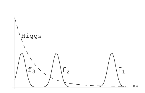
Figure 3.2: Locations and profiles of fermion wave functions in the fifth dimension with an exponentially decaying Higgs; here only one fermion per family is displayed.

In fact we see that the left and right wave functions of heavy quarks have a greater overlap than the ones of light quarks, the latter being located farer from each others in the extra dimension. If we relax the hypothesis of constant Higgs we can also obtain the correct mass spectrum with only three localization points, one per generation. For instance this can be achieved with an exponentially decaying Higgs (see fig. 3.2) [40]. In both cases there is an exponential mapping between the parameters of the higher-dimensional theory and the 4D masses and mixing angles, so that even with parameters of order one large hierarchies are created. The number of parameters we need is not lowered, but now they are all of the same magnitude.

In orbifold compactifications, solitons are simulated by scalar fields with a non-trivial parity assignment that forbids constant non-vanishing vevs. Under certain conditions, the energy is minimized by field configurations with a non-trivial dependence upon the compact coordinates [42]. As an example we consider the orbifold $M^{4}\times S^{1}/\mathbb{Z}_{2}$ and we choose $\psi_{L}(\psi_{R})$ even(odd) under $\mathbb{Z}_{2}$ and $\phi$ odd, from which it follows that $\int du\,\phi(u)$ is even. If then we calculate the zero modes we see from eq. (3.3) that only $\psi_{L}$ is acceptable: $\psi_{R}$ would be even, contrary to the initial assignment. In particular if we choose $\phi(x_{5})=\epsilon(x_{5})$, where $\epsilon(x_{5})$ is now the periodic sign function, we obtain:

$$\psi_{L}(x,x_{5})\propto e^{\displaystyle{-g|x_{5}|_{per}}}\leavevmode\nobreak\ \psi_{L}(x)\leavevmode\nobreak\ .$$ (3.5)

$\psi_{L}$ is localized at $x_{5}=0$ or at $x_{5}=\pi R$ depending on the sign of $g$. Also in this case we have obtained a chiral localized zero mode, but while with an infinite extra dimension it was the normalization making the theory chiral, here it is a consequence of orbifold projection.

In models like the ones described above, from one higher-dimensional spinor we get one 4D chiral zero mode. Is it possible to obtain as many chiral fermions as we want starting from one single higher-dimensional spinor? The answer to this question was given already in the 80’s (see refs. [37]) when it had been shown that coupling a fermion to a topologically non-trivial background could produce a number of zero modes related to the topology of the background itself. Recently these results have been re-derived in a more phenomenological context. For instance, in the model studied in ref. [43], the authors consider a topological defect in two infinite extra dimensions whose core corresponds to our 4D world. Chiral fermion zero modes are trapped in the core by specific interactions with the vortex of winding number $k$ which builds up the defect. In this case an index theorem guarantees that the number of chiral zero modes is equal to the topological charge $k$. Starting from one single 6D spinor and choosing $k=3$ they obtain three 4D fermion species with identical gauge and global quantum number, which differ among themselves only in the dependence on the extra coordinates. If we trap in the core the Higgs field by coupling it to the vortex, his overlap with different fermion functions generates the observed hierarchy of masses. To obtain the correct mixing angles the model has to be complicated a little by introducing another scalar field which, combined with the first one, builds up a new defect. Although this model is not very simple, it gives an answer both to the flavour problem and to the question of the number of families. Recently it has been extended to the case of two extra dimensions compactified on a sphere [44]. A compact extra space has the advantage of localizing the gauge fields in a finite region.

Among the previously discussed models only the latter try to give an explanation of the origin of fermion replica. Then one may think that only with the introduction of a topological defect it is possible to address both the issues. This is not true. It is well known in fact that a spinor in $d$ dimensions have $2^{[d/2]}$ complex components, that means it can contain many 4D replica. In 5D a fermion contains two 4D components with opposite chirality; after projecting out the wrong chirality, for example with an orbifold projection, we are left with a single generation. One extra dimension is then not enough to our purpose. In 6D fermions can be chiral and a 6D chiral fermion has the same content of a 5D fermion. If we consider a 6D vector-like fermion and we project out through orbifolding the unwanted chirality we are left with two replica with the same chirality and the same quantum numbers. In order to have a realistic model we need three families, so also two extra dimensions are not enough. But in order to understand if this kind of models can account both for the mass hierarchy and the flavour mixing and how this can work, we can begin to explore this simplified case. This has been done in ref. [45] where the authors proposed a 6D toy model that we describe in the following section.

3.2 A Toy Model for Two Generations

3.2.1 Localized Fermions

We consider two extra spatial dimensions compactified on the orbifold $T^{2}/\mathbb{Z}_{2}$, where $T^{2}$ is the torus defined by $x_{i}\to x_{i}+2\pi R_{i}$ $(i=5,6)$ and $\mathbb{Z}_{2}$ is the parity symmetry $(x_{5},x_{6})\to(-x_{5},-x_{6})$. As fundamental region of the orbifold we can take, for instance, the rectangle $(|x_{5}|\leq\pi R_{5})$, $(0\leq x_{6}\leq\pi R_{6})$ (see fig. 3.3).

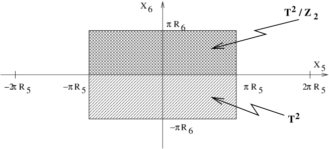
Figure 3.3: Fundamental region of the orbifold $T^{2}/\mathbb{Z}_{2}$.

There are four inequivalent fixed points under $\mathbb{Z}_{2}$. In the chosen fundamental region they can be identified with $(x_{5},x_{6})=(0,0)$, $(\pi R_{5},0)$, $(0,\pi R_{6})$, $(\pi R_{5},\pi R_{6})$.

Since we want to reproduce the SM, we ask invariance under the gauge group SU(3)$\otimes$SU(2)$\otimes$U(1). As discussed in the previous section, we want to end with two fermion replica, so that we need to start with vector-like fermions. To justify this choice we also ask invariance under 6D parity. As a consequence, the lagrangian has 6D vector-like fermions $\Psi^{(\alpha)}$ $(\alpha=1,...5)$, one for each irreducible representation of the SM, as summarized in table 3.1. With this set of fermion fields, our model is automatically free from 6D gauge anomalies. As we will see later on, requiring exact 6D parity symmetry is too strong an assumption to obtain a ‘realistic’ fermion spectrum. Although eventually we will relax this assumption, for the time being we carry on our construction by enforcing 6D parity invariance.

field	SU(3)	SU(2)	U(1)
$\Psi^{(1)}$	3	2	+1/6
$\Psi^{(2)}$	3	1	+2/3
$\Psi^{(3)}$	3	1	-1/3
$\Psi^{(4)}$	1	2	-1/2
$\Psi^{(5)}$	1	1	-1

Table 3.1: Vector-like 6D fermions and their gauge quantum numbers.

We have:

$${\cal L}_{g}={\cal L}_{gauge}+i\sum_{\alpha=1}^{5}\overline{\Psi^{(\alpha)}}\Gamma^{M}D_{M}\Psi^{(\alpha)}\leavevmode\nobreak\ ,$$ (3.6)

where ${\cal L}_{gauge}$ stands for the 6D kinetic term for the gauge vector bosons $A_{M}$ $(M=\mu;i=0,...3;5,6)$ of SU(3)$\otimes$SU(2)$\otimes$U(1), $\Gamma^{M}$ are the 6D gamma matrices and $D_{M}\Psi^{(\alpha)}$ denotes the appropriate fermion covariant derivative. We recall that, up to the $(x_{5},x_{6})$ dependence, a 6D vector-like spinor is equivalent to a pair of 4D Dirac spinors: $\Psi=(\eta,\chi)^{T}$. Moreover each 6D fermion can be split into two chiralities $\Psi=\Psi_{+}+\Psi_{-}$, eigenstates of $\Gamma_{7}$: $\Psi_{\pm}=(1\pm\Gamma_{7})/2\leavevmode\nobreak\ \leavevmode\nobreak\ \Psi$. We choose a representation for the Dirac matrices in 6D where $\Gamma_{7}=\gamma_{5}\otimes\sigma_{3}$ (see appendix A), where $\sigma_{3}$ is the third Pauli matrix, so that in terms of 4D chiralities we have: $\Psi_{+}=(\eta_{R},\chi_{L})^{T}$ and $\Psi_{-}=(\eta_{L},\chi_{R})^{T}$. Each component $\eta_{L,R}$, $\chi_{L,R}$ transforms in the same way under the gauge group. All fields are assumed to be periodic in $x_{5}$ and $x_{6}$. By inspecting the kinetic terms, we see that consistency with the orbifold projection requires a non-trivial assignment of the $\mathbb{Z}_{2}$ parity. We take $A_{\mu}$ even under $\mathbb{Z}_{2}$ and $A_{i}$ $\mathbb{Z}_{2}$-odd. In the fermion sector, $\eta_{R(L)}$ and $\chi_{R(L)}$ should have the same $\mathbb{Z}_{2}$ parity, which should be opposite for $\eta_{R(L)}$ and $\chi_{L(R)}$. We choose $\mathbb{Z}_{2}(\eta^{(\alpha)}_{R},\chi^{(\alpha)}_{L},\eta^{(\alpha)}_{L},\chi^{(\alpha)}_{R})$ equal to $(-1,+1,+1,-1)$ for $\alpha=1,4$, and $(+1,-1,-1,+1)$ for $\alpha=2,3,5$. At this level the zero modes are the gauge vector bosons of the SM and two independent chiral fermions for each irreducible representation of the SM, describing two massless generations. There are no gauge anomalies in our model. Bulk anomalies are absent because the 6D fermions are vector-like. There could be gauge 4D anomalies localized at the four orbifold fixed points [46, 47]. In our model based on $T^{2}/\mathbb{Z}_{2}$, the anomalies are the same at each fixed point and they actually vanish with the quantum number assignments of table 3.1. Indeed they are proportional to the anomalies of the 4D zero modes, which form two complete fermion generations, thus providing full 4D anomaly cancellation. Fermion masses in 6D and Yukawa couplings do not modify this conclusion.

In the absence of additional interactions, each zero mode is constant with respect to $x_{5}$ and $x_{6}$. Even by introducing a 6D (parity invariant) Yukawa interaction between fermions and a Higgs electroweak doublet, we do not break the 4D flavor symmetry, which is maximal. The first step to distinguish the two fermion generations is to localize them in different regions of the compact space. In our model this can be done in a very simple way, by introducing a 6D fermion mass term

$${\cal L}_{m} = \sum_{\alpha=1}^{5}m_{(\alpha)}\overline{\Psi^{(\alpha)}}\Psi^{(\alpha)}$$ (3.7)

$$= \sum_{\alpha=1}^{5}m_{(\alpha)}\overline{\Psi^{(\alpha)}}\left(\frac{1-\Gamma_{7}}{2}\right)\Psi^{(\alpha)}+h.c.\leavevmode\nobreak\ ,$$

where 6D parity requires $m_{(\alpha)}$ to be real. This term is gauge invariant and relates left and right 4D chiralities. Therefore the mass parameters $m_{(\alpha)}$ are required to be $\mathbb{Z}_{2}$-odd and cannot be constant in the whole $(x_{5},x_{6})$ plane. The simplest possible choice for $m_{(\alpha)}$ is a constant in the orbifold fundamental region:

$$m_{(\alpha)}(x_{5},x_{6})=\mu_{(\alpha)}\epsilon(x_{6})\leavevmode\nobreak\ ,$$ (3.8)

where $\epsilon(x_{6})$ denotes the (periodic) sign function. This function can be regarded as a background field. In a more fundamental theory it could arise dynamically from the vev of a gauge singlet scalar field, periodic and $\mathbb{Z}_{2}$-odd [42]. Then the parameters $\mu_{(\alpha)}$ would essentially represent Yukawa couplings. In our toy model we regard $\epsilon(x_{6})$ as an external fixed background and neglect its dynamics.

The properties of the 4D light fermions are now described by the zero modes of the 4D Dirac operator in the background proportional to $\epsilon(x_{6})$. These zero modes are the normalized solutions to the differential equations:

$$(\partial_{5}+i\partial_{6})\chi^{(\alpha)}_{L}+\mu_{(\alpha)}\epsilon(x_{6})\eta^{(\alpha)}_{L} = 0$$

$$(\partial_{5}-i\partial_{6})\eta^{(\alpha)}_{L}+\mu_{(\alpha)}^{*}\epsilon(x_{6})\chi^{(\alpha)}_{L} = 0$$

$$-(\partial_{5}+i\partial_{6})\chi^{(\alpha)}_{R}+\mu_{(\alpha)}^{*}\epsilon(x_{6})\eta^{(\alpha)}_{R} = 0$$

$$-(\partial_{5}-i\partial_{6})\eta^{(\alpha)}_{R}+\mu_{(\alpha)}\epsilon(x_{6})\chi^{(\alpha)}_{R} = 0\leavevmode\nobreak\ ,$$ (3.9)

with periodic boundary conditions for all fields and with the $\mathbb{Z}_{2}$ parities defined above. Combining eqs. (3.9) together we obtain the following second order partial differential equations, holding in the whole $(x_{5},x_{6})$ plane:

$$(\partial_{5}^{2}+\partial_{6}^{2})\ \chi_{L}^{\alpha}-|\mu_{(\alpha)}|^{2}\ \epsilon^{2}(x_{6})\ \chi_{L}^{\alpha}-2\ i\ \mu_{(\alpha)}\ (-1)^{k}\ \delta_{k}(x_{6})\ \eta_{L}^{\alpha} = 0$$

$$(\partial_{5}^{2}+\partial_{6}^{2})\ \eta_{L}^{\alpha}-|\mu_{(\alpha)}|^{2}\ \epsilon^{2}(x_{6})\ \eta_{L}^{\alpha}+2\ i\ \mu_{(\alpha)}^{*}\ (-1)^{k}\ \delta_{k}(x_{6})\ \chi_{L}^{\alpha} = 0$$

$$(\partial_{5}^{2}+\partial_{6}^{2})\ \chi_{R}^{\alpha}-|\mu_{(\alpha)}|^{2}\ \epsilon^{2}(x_{6})\ \chi_{R}^{\alpha}+2\ i\ \mu_{(\alpha)}^{*}\ (-1)^{k}\ \delta_{k}(x_{6})\ \eta_{R}^{\alpha} = 0$$

$$(\partial_{5}^{2}+\partial_{6}^{2})\ \eta_{R}^{\alpha}-|\mu_{(\alpha)}|^{2}\ \epsilon^{2}(x_{6})\ \eta_{R}^{\alpha}-2\ i\ \mu_{(\alpha)}\ (-1)^{k}\ \delta_{k}(x_{6})\ \chi_{R}^{\alpha} = 0$$ (3.10)

where $k$ is an integer, $\delta_{k}(x_{6})\equiv\delta(x_{6}-k\pi R_{6})$ and the sum over $k$ is understood. The advantage of working with eqs. (3.10) is that in the bulk these equations are decoupled and identical for all fields. Away from the lines $x_{6}=k\pi R_{6}$, $k\in\mathbb{Z}$, they read:

$$(\partial_{5}^{2}+\partial_{6}^{2})\ \phi-|\mu_{(\alpha)}|^{2}\ \phi=0$$ (3.11)

with appropriate boundary conditions. Here $\phi$ stands for $\chi_{L}^{\alpha}$, $\eta_{L}^{\alpha}$, $\chi_{R}^{\alpha}$, $\eta_{R}^{\alpha}$. In each strip $k\pi R_{6}<x_{6}<(k+1)\pi R_{6}$, the general solution to this equation can be written in the form:

$$\phi^{(k)}(x,x_{5},x_{6})=\sum_{n\in\mathbb{Z}}\ \left[\ C^{(k)}_{n}(x)\ e^{\displaystyle\alpha_{n}\frac{x_{6}}{R_{5}}}+C^{\prime(k)}_{n}(x)\ e^{\displaystyle-\alpha_{n}\frac{x_{6}}{R_{5}}}\ \right]\ e^{\displaystyle in\frac{x_{5}}{R_{5}}}$$ (3.12)

with $\alpha_{n}=\sqrt{n^{2}+|\mu_{\alpha}|^{2}R_{5}^{2}}$. These solutions can be glued together by imposing periodicity along $x_{6}$, $\mathbb{Z}_{2}$ parity and the appropriate discontinuity across the lines $x_{6}=k\pi R_{6}$. This last requirement can be directly derived from eqs. (3.9) and eqs. (3.10). The fields $\phi$ should be continuous everywhere, whereas their first derivatives have discontinuities $\Delta^{(k)}(\partial_{6}\phi)$ given by:

$$\begin{array}[]{ll}\Delta^{(2k)}(\partial_{6}\phi)=-2\,i\,s(\phi^{\prime})\,\phi^{\prime}(2k\pi R_{6})&\textrm{at}\quad x_{6}=2k\pi R_{6}\\ \Delta^{(2k+1)}(\partial_{6}\phi)=2\,i\,s(\phi^{\prime})\,\phi^{\prime}((2k+1)\pi R_{6})&\textrm{at}\quad x_{6}=(2k+1)\pi R_{6}\end{array}$$ (3.13)

where $(\phi,\phi^{\prime})=(\chi_{L}^{\alpha},\eta_{L}^{\alpha}),\,(\eta_{L}^{\alpha},\chi_{L}^{\alpha}),\,(\chi_{R}^{\alpha},\eta_{R}^{\alpha}),\,(\eta_{R}^{\alpha},\chi_{R}^{\alpha})$ and

$$s(\phi^{\prime})=\left\{\begin{array}[]{ll}-\mu_{\alpha}&\textrm{if}\ \phi^{\prime}=\eta_{L}^{\alpha},\,\chi_{R}^{\alpha}\\ \mu_{\alpha}^{*}&\textrm{if}\ \phi^{\prime}=\eta_{R}^{\alpha},\,\chi_{L}^{\alpha}\end{array}\right.\leavevmode\nobreak\ .$$ (3.14)

These requirements have a non-trivial solution only for $n=0$, that means the zero modes are independent of $x_{5}$. We obtain:

• $\alpha=1,4$

$$\left(\begin{array}[]{c}\eta^{(\alpha)}_{R}\\ \chi^{(\alpha)}_{R}\end{array}\right) = 0$$ (3.17)

$$\left(\begin{array}[]{c}\eta^{(\alpha)}_{L}\\ \chi^{(\alpha)}_{L}\end{array}\right) = f^{(\alpha)}_{1}(x)\left(\begin{array}[]{c}1\\ i\displaystyle\frac{\mu_{(\alpha)}}{|\mu_{(\alpha)}|}\end{array}\right)\xi^{(\alpha)}_{1}(x_{5},x_{6})+f^{(\alpha)}_{2}(x)\left(\begin{array}[]{c}1\\ -i\displaystyle\frac{\mu_{(\alpha)}}{|\mu_{(\alpha)}|}\end{array}\right)\xi^{(\alpha)}_{2}(x_{5},x_{6})\leavevmode\nobreak\ ,$$ (3.24)

• $\alpha=2,3,5$

$$\left(\begin{array}[]{c}\eta^{(\alpha)}_{R}\\ \chi^{(\alpha)}_{R}\end{array}\right) = f^{(\alpha)}_{1}(x)\left(\begin{array}[]{c}1\\ -i\displaystyle\frac{\mu_{(\alpha)}^{\leavevmode\nobreak\ *}}{|\mu_{(\alpha)}|}\end{array}\right)\xi^{(\alpha)}_{1}(x_{5},x_{6})+f^{(\alpha)}_{2}(x)\left(\begin{array}[]{c}1\\ i\displaystyle\frac{\mu_{(\alpha)}^{\leavevmode\nobreak\ *}}{|\mu_{(\alpha)}|}\end{array}\right)\xi^{(\alpha)}_{2}(x_{5},x_{6})$$ (3.31)

$$\left(\begin{array}[]{c}\eta^{(\alpha)}_{L}\\ \chi^{(\alpha)}_{L}\end{array}\right) = 0\leavevmode\nobreak\ ,$$ (3.34)

where $f^{(\alpha)}_{1,2}(x)$ are 4D chiral spinors:

$$\begin{array}[]{ll}f^{(1)}_{1}=\left(\begin{array}[]{c}u_{L}\\ d_{L}\end{array}\right)&\leavevmode\nobreak\ \leavevmode\nobreak\ \leavevmode\nobreak\ \leavevmode\nobreak\ \leavevmode\nobreak\ f^{(1)}_{2}=\left(\begin{array}[]{c}c_{L}\\ s_{L}\end{array}\right)\\ f^{(2)}_{1}=u_{R}&\leavevmode\nobreak\ \leavevmode\nobreak\ \leavevmode\nobreak\ \leavevmode\nobreak\ \leavevmode\nobreak\ f^{(2)}_{2}=c_{R}\\ f^{(3)}_{1}=d_{R}&\leavevmode\nobreak\ \leavevmode\nobreak\ \leavevmode\nobreak\ \leavevmode\nobreak\ \leavevmode\nobreak\ f^{(3)}_{2}=s_{R}\\ f^{(4)}_{1}=\left(\begin{array}[]{c}\nu_{eL}\\ e_{L}\end{array}\right)&\leavevmode\nobreak\ \leavevmode\nobreak\ \leavevmode\nobreak\ \leavevmode\nobreak\ \leavevmode\nobreak\ f^{(4)}_{2}=\left(\begin{array}[]{c}\nu_{\mu L}\\ \mu_{L}\end{array}\right)\\ f^{(5)}_{1}=e_{R}&\leavevmode\nobreak\ \leavevmode\nobreak\ \leavevmode\nobreak\ \leavevmode\nobreak\ \leavevmode\nobreak\ f^{(5)}_{2}=\mu_{R}\end{array}\leavevmode\nobreak\ ,$$

whereas $\xi^{(\alpha)}_{1,2}(x_{5},x_{6})$ are functions describing the localization of the zero modes in the compact space:

$$\xi^{(\alpha)}_{1}(x_{5},x_{6}) = \frac{e^{\displaystyle{-\pi|\mu_{(\alpha)}|R_{6}}}}{\sqrt{2\pi R_{5}}}\leavevmode\nobreak\ \frac{\sqrt{|\mu_{(\alpha)}|}}{\sqrt{1-e^{\displaystyle{-2\pi|\mu_{(\alpha)}|R_{6}}}}}\leavevmode\nobreak\ \leavevmode\nobreak\ e^{\leavevmode\nobreak\ \displaystyle{|\mu_{(\alpha)}x_{6}|_{per}}}$$

$$\xi^{(\alpha)}_{2}(x_{5},x_{6}) = \frac{1}{\sqrt{2\pi R_{5}}}\leavevmode\nobreak\ \frac{\sqrt{|\mu_{(\alpha)}|}}{\sqrt{1-e^{\displaystyle{-2\pi|\mu_{(\alpha)}|R_{6}}}}}\leavevmode\nobreak\ \leavevmode\nobreak\ e^{\displaystyle{-|\mu_{(\alpha)}x_{6}|_{per}}}\leavevmode\nobreak\ .$$ (3.35)

In the above equations $|x_{6}|_{per}$ denotes a periodic function, coinciding with the ordinary $|x_{6}|$ in the interval $[-\pi R_{6},\pi R_{6}]$. As in the case $m_{(\alpha)}=0$, for each 6D spinor we have two independent chiral zero modes, whose 4D dependence is described by $f^{(\alpha)}_{1,2}$. They are still constant in $x_{5}$, but not in $x_{6}$.

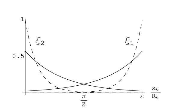
Figure 3.4: Wave functions $\xi^{(\alpha)}_{1,2}(x_{5},x_{6})$, in units of $\sqrt{R_{5}R_{6}}$. They have been obtained by choosing $|\mu_{(\alpha)}|R_{6}=1(3)$ for continuous(dashed) lines.

Indeed, the zero mode proportional to $f^{(\alpha)}_{2}$ is localized at $x_{6}=0$ (mod $2\pi R_{6}$), whereas that proportional to $f^{(\alpha)}_{1}$ is peaked around $x_{6}=\pi R_{6}$ (mod $2\pi R_{6}$) (see fig. 3.4). The two zero modes with well-defined localization properties in the compact space have non-trivial components both along $\eta$ and along $\chi$ and they are orthogonal to each other. The constant factors in eqs. (3.35) normalize the zero modes to 1. In our toy model, the number of zero modes is not related to a non-trivial topological property of the background $\epsilon(x_{6})$. The two zero modes are determined by the orbifold projection. The presence of the background only induces a separation of the corresponding wave functions in the compact space. Actually we can go smoothly from localized to constant wave functions, by turning off the constants $\mu_{(\alpha)}$, as apparent from eqs. (3.35).

With the introduction of the background, we now have two fermion generations, one sat at $x_{6}=0$ and the other at $x_{6}=\pi R_{6}$. From the point of view of the 4D observer, who cannot resolve distances in the extra space, there is still a maximal flavour symmetry and, indeed, all fermions are still massless at this level. Fermions can acquire masses in the usual way, by breaking the electroweak symmetry via the non-vanishing vev of a Higgs doublet $H$. If such a vev were a constant in $x_{6}$, then we would obtain equal masses for the two fermion generations. Thus, to break the 4D flavour symmetry we need a non-trivial dependence of the Higgs vev upon $x_{6}$. There are several ways to achieve this. For instance, we might assume that $H$ is a bulk field. Under certain conditions it may happen that the minimum of the energy is no longer $x_{6}$-constant. Examples of this kind are well-known in the literature [48]. If $H$ interacts with a suitable $x_{6}$-dependent background, there is a competition between the kinetic energy term, which prefers constant configurations, and the potential energy term, which may favour a $x_{6}$-varying vev. In non-vanishing portions of the parameter space the minimum of the energy can depend non-trivially on $x_{6}$. In the minimal version of our toy model we will simulate this dependence in the simplest possible way, by introducing a Higgs doublet $H$ with hypercharge +1/2 localized along the line $x_{6}=0$. The most general Yukawa interaction term invariant under $\mathbb{Z}_{2}$, 6D parity and SU(3) $\otimes$ SU(2) $\otimes$ U(1) reads:

$${\cal L}_{Y}=\left[y_{u}\leavevmode\nobreak\ \tilde{H}^{\dagger}\leavevmode\nobreak\ \overline{\Psi^{(2)}}\Psi^{(1)}+y_{d}\leavevmode\nobreak\ H^{\dagger}\leavevmode\nobreak\ \overline{\Psi^{(3)}}\Psi^{(1)}+y_{e}\leavevmode\nobreak\ H^{\dagger}\leavevmode\nobreak\ \overline{\Psi^{(5)}}\Psi^{(4)}+h.c.\right]\delta(x_{6})\leavevmode\nobreak\ ,$$ (3.36)

where $\tilde{H}=i\sigma^{2}H^{*}$. Notice that $H$ has dimension +3/2 and $y$ has dimension -3/2, in mass units. In the next section we will see how a realistic pattern of masses and mixing angles arises from these Yukawa interactions.

Summarizing, our model is described by the lagrangian:

$${\cal L}={\cal L}_{g}+{\cal L}_{m}+{\cal L}_{Y}+{\cal L}_{H}\leavevmode\nobreak\ ,$$ (3.37)

where ${\cal L}_{g}$, ${\cal L}_{m}$, ${\cal L}_{Y}$ are given in eqs. (3.6), (3.7) and (3.36), respectively, while ${\cal L}_{H}$, localized at $x_{6}=0$, contains the kinetic term for the Higgs doublet and the scalar potential that breaks spontaneously SU(2)$\otimes$U(1). The complex phases in $y_{i}$ can be completely eliminated via field redefinitions: in the limit of exact 6D parity symmetry all parameters are real.

3.2.2 Masses and Mixing Angles

The fermion mass terms arise from ${\cal L}_{Y}$ after ESB, here described by $\langle H\rangle=(0\leavevmode\nobreak\ v/\sqrt{2})^{T}$. To evaluate the fermion mass matrices we should expand the 6D fermion fields in 4D modes and then perform the $x_{5}$ and $x_{6}$ integrations. In practice, if we focus on the lightest sector, we can keep only the zero modes in the expansion. We obtain:

$$m_{u} = \frac{y_{u}}{\sqrt{2}}\leavevmode\nobreak\ v\leavevmode\nobreak\ \frac{\sqrt{|\mu_{(1)}\mu_{(2)}|}}{2\sqrt{(1-\lambda_{1}^{2})(1-\lambda_{2}^{2})}}\left(\begin{array}[]{cc}c_{u-}\leavevmode\nobreak\ \lambda_{1}\lambda_{2}&c_{u+}\leavevmode\nobreak\ \lambda_{2}\\ c_{u+}\leavevmode\nobreak\ \lambda_{1}&c_{u-}\end{array}\right)$$ (3.40)

$$m_{d} = \frac{y_{d}}{\sqrt{2}}\leavevmode\nobreak\ v\leavevmode\nobreak\ \frac{\sqrt{|\mu_{(1)}\mu_{(3)}|}}{2\sqrt{(1-\lambda_{1}^{2})(1-\lambda_{3}^{2})}}\left(\begin{array}[]{cc}c_{d-}\leavevmode\nobreak\ \lambda_{1}\lambda_{3}&c_{d+}\leavevmode\nobreak\ \lambda_{3}\\ c_{d+}\leavevmode\nobreak\ \lambda_{1}&c_{d-}\end{array}\right)$$ (3.43)

$$m_{e} = \frac{y_{e}}{\sqrt{2}}\leavevmode\nobreak\ v\leavevmode\nobreak\ \frac{\sqrt{|\mu_{(4)}\mu_{(5)}|}}{2\sqrt{(1-\lambda_{4}^{2})(1-\lambda_{5}^{2})}}\left(\begin{array}[]{cc}c_{e-}\leavevmode\nobreak\ \lambda_{4}\lambda_{5}&c_{e+}\leavevmode\nobreak\ \lambda_{5}\\ c_{e+}\leavevmode\nobreak\ \lambda_{4}&c_{e-}\end{array}\right)\leavevmode\nobreak\ ,$$ (3.46)

where

$$c_{u\pm}=1\pm\frac{\mu_{(1)}\mu_{(2)}}{|\mu_{(1)}\mu_{(2)}|}\leavevmode\nobreak\ ,\leavevmode\nobreak\ \leavevmode\nobreak\ \leavevmode\nobreak\ \leavevmode\nobreak\ \leavevmode\nobreak\ \leavevmode\nobreak\ c_{d\pm}=1\pm\frac{\mu_{(1)}\mu_{(3)}}{|\mu_{(1)}\mu_{(3)}|}\leavevmode\nobreak\ ,\leavevmode\nobreak\ \leavevmode\nobreak\ \leavevmode\nobreak\ \leavevmode\nobreak\ \leavevmode\nobreak\ \leavevmode\nobreak\ c_{e\pm}=1\pm\frac{\mu_{(4)}\mu_{(5)}}{|\mu_{(4)}\mu_{(5)}|}\leavevmode\nobreak\ ,$$ (3.47)

and

$$\lambda_{\alpha}=e^{\displaystyle{-\pi|\mu_{(\alpha)}|R_{6}}}\leavevmode\nobreak\ .$$ (3.48)

These mass matrices, here given in the convention $\overline{f_{R}}m_{f}f_{L}$, are not hermitian. It is interesting to see that, for generic order-one values of the dimensionless combinations $c_{f\pm}$ and $\mu_{(\alpha)}R_{6}$, the mass matrices display a clear hierarchical pattern. Fermion masses of the first generation are suppressed by $\lambda_{(\alpha)}\lambda_{(\beta)}$ compared to those of the second generation and mixing angles are of order $\lambda_{(\alpha)}$ or $\lambda_{(\beta)}$. This is quite similar to what obtained in 4D models with a spontaneously broken flavour symmetry. Here the rôle of small expansion parameters is played by the quantities $\lambda_{\alpha}$. However in our parity invariant model, the parameters $\mu_{(\alpha)}$ are real and the coefficients $c_{f\pm}$ are ‘quantized’. Either $c_{f+}$ or $c_{f-}$ should vanish and this implies no mixing. Indeed when 6D parity is conserved, we have only two possible orientations of the fermion zero modes in the $(\eta,\chi)$ space: either $(1,i)$ or $(1,-i)$, as apparent from eqs. (3.17) and (3.34). Thus the scalar product between two zero modes in the $(\eta,\chi)$ space is either maximal or zero. Modulo a relabeling among first and second generations, this gives rise to a perfect alignment of mass matrices and a vanishing overall mixing. To overcome this problem, we should relax the assumption of exact 6D parity symmetry. We will assume that 6D parity is broken ‘softly’, by the fermion-background interaction described by ${\cal L}_{m}$. This can be achieved by taking complex values for the mass coefficients $\mu_{(\alpha)}$. In a fundamental theory such a breaking could be spontaneous: if $m_{(\alpha)}$ were complex fields, then the lagrangian would still be invariant under 6D parity acting as $m_{(\alpha)}\leftrightarrow m_{(\alpha)}^{\dagger}$. It might occur that the dynamics of the fields $m_{(\alpha)}$ led to complex vevs for $m_{(\alpha)}$, thus spontaneously breaking parity. In our toy model we will simply assume the existence of such a complex background. All the relations that we have derived hold true for the complex case as well and we have now hierarchical mass matrices with a non-trivial intergenerational mixing. By expanding the results at leading order in $\lambda_{\alpha}$ we find:

$$m_{c}=|y_{u}|v\frac{\sqrt{|\mu_{(1)}\mu_{(2)}|}}{2\sqrt{2}}|c_{u-}|\leavevmode\nobreak\ \leavevmode\nobreak\ \leavevmode\nobreak\ \leavevmode\nobreak\ \leavevmode\nobreak\ \leavevmode\nobreak\ \leavevmode\nobreak\ \leavevmode\nobreak\ {\displaystyle\frac{m_{u}}{m_{c}}=\frac{|c_{u+}^{2}-c_{u-}^{2}|}{|c_{u-}|^{2}}\lambda_{1}\lambda_{2}}$$

$$m_{s}=|y_{d}|v\frac{\sqrt{|\mu_{(1)}\mu_{(3)}|}}{2\sqrt{2}}|c_{d-}|\leavevmode\nobreak\ \leavevmode\nobreak\ \leavevmode\nobreak\ \leavevmode\nobreak\ \leavevmode\nobreak\ \leavevmode\nobreak\ \leavevmode\nobreak\ \leavevmode\nobreak\ {\displaystyle\frac{m_{d}}{m_{s}}=\frac{|c_{d+}^{2}-c_{d-}^{2}|}{|c_{d-}|^{2}}\lambda_{1}\lambda_{3}}$$

$$m_{\mu}=|y_{e}|v\frac{\sqrt{|\mu_{(4)}\mu_{(5)}|}}{2\sqrt{2}}|c_{e-}|\leavevmode\nobreak\ \leavevmode\nobreak\ \leavevmode\nobreak\ \leavevmode\nobreak\ \leavevmode\nobreak\ \leavevmode\nobreak\ \leavevmode\nobreak\ \leavevmode\nobreak\ \leavevmode\nobreak\ \leavevmode\nobreak\ {\displaystyle\frac{m_{e}}{m_{\mu}}=\frac{|c_{e+}^{2}-c_{e-}^{2}|}{|c_{e-}|^{2}}\lambda_{4}\lambda_{5}}\leavevmode\nobreak\ .$$ (3.49)

Finally, after absorbing residual phases in the definition of the $s$ and $c$ 4D fields, the matrices $m_{u}^{\dagger}m_{u}$ and $m_{d}^{\dagger}m_{d}$ are diagonalized by orthogonal transformations characterized by mixing angles $\theta_{u,d}$:

$$\theta_{u,d}=\left|\frac{c_{u,d+}}{c_{u,d-}}\right|\lambda_{1}\leavevmode\nobreak\ ,$$ (3.50)

still at leading order in $\lambda_{\alpha}$. Therefore the Cabibbo angle is given by:

$$\theta_{C}=\left(\left|\frac{c_{d+}}{c_{d-}}\right|-\left|\frac{c_{u+}}{c_{u-}}\right|\right)\lambda_{1}\leavevmode\nobreak\ .$$ (3.51)

Barring accidental cancellations in the relevant combinations of the coefficients $c_{f\pm}$, the Cabibbo angle is of order $\lambda_{1}$. Then, by assuming $\lambda_{3}\approx\lambda_{1}$ and $\lambda_{2}\approx\lambda_{1}^{3}$ we reproduce the correct order of magnitude of mass ratios in the quark sector. These are small numbers in the 4D theory, but can be obtained quite naturally from the 6D point of view: $\mu_{(1)}R_{6}\approx\mu_{(3)}R_{6}\approx 0.5$ and $\mu_{(2)}R_{6}\approx 1.3$. Similarly, by taking $\lambda_{4}\lambda_{5}\approx\lambda_{1}^{2}$ we can naturally fit the lepton mass ratio.

It can be useful to comment about the way flavour symmetry is broken in this toy model. Before the introduction of the Yukawa interactions and modulo U(1) anomalies, the flavour symmetry group is U(2)⁵. After turning the Yukawa couplings on, we can consider several limits. When $R_{6}\to\infty$, the quantities $\lambda_{(\alpha)}$ vanish and the flavour symmetry is broken down to U(1)⁵, acting non-trivially on the lightest sector. If $R_{6}$ is finite and non-vanishing, U(1)⁵ is in turn completely broken down by $\lambda_{(\alpha)}\neq 0$. Nevertheless, contrary to what happens in models with abelian flavour symmetries, the coefficients of order one that multiply the symmetry breaking parameters $\lambda_{(\alpha)}$ are now related one to each other. This can be appreciated by taking the limit $R_{6}\to 0$. We have $\lambda_{(\alpha)}=1$ and the residual flavour symmetry is a permutation symmetry, separately for the lepton and the quark sectors: $S_{2}\otimes S_{2}$.

Let us now briefly comment about neutrino masses and mixings in this set-up. The most straightforward way to produce neutrino masses is to add a gauge singlet 6D fermion field, $\Psi^{(6)}$, with $\mathbb{Z}_{2}$ assignments $(+1,-1,-1,+1)$. As for the case of charged fermions, by introducing a mass term for $\Psi^{(6)}$ as in eq. (3.7) and a Yukawa interaction with $\Psi^{(4)}$ and $\tilde{H}$ as in eq. (3.36), we obtain a Dirac neutrino mass term

$$m_{\nu}=\frac{y_{\nu}}{\sqrt{2}}v\frac{\sqrt{|\mu_{(4)}\mu_{(6)}|}}{2\sqrt{(1-\lambda_{4}^{2})(1-\lambda_{6}^{2})}}\left(\matrix{c_{\nu-}\lambda_{4}\lambda_{6}&c_{\nu+}\lambda_{6}\cr c_{\nu+}\lambda_{4}&c_{\nu-}}\right)\leavevmode\nobreak\ .$$ (3.52)

A large mixing angle in the lepton sector, $\theta_{L}$, is obtained for $\lambda_{4}=O(1)$, in which case the neutrino mass hierarchy,

$$\frac{m_{\nu_{1}}}{m_{\nu_{2}}}=\frac{|c_{\nu+}^{2}-c_{\nu-}^{2}|}{|c_{\nu-}|^{2}}\lambda_{4}\lambda_{6}\leavevmode\nobreak\ ,$$ (3.53)

is controlled by $\lambda_{6}$. At leading order, the left mixings in $m_{e}^{\dagger}m_{e}$ and $m_{\nu}^{\dagger}m_{\nu}$ correspond to

$$\tan 2\theta_{e,\nu}=\frac{2\leavevmode\nobreak\ c_{e,\nu+}\leavevmode\nobreak\ c_{e,\nu-}\leavevmode\nobreak\ \lambda_{4}}{(c_{e,\nu-}^{2}-c_{e,\nu+}^{2}\leavevmode\nobreak\ \lambda_{4}^{2})}\leavevmode\nobreak\ ,$$ (3.54)

so that $\theta_{L}\equiv\theta_{\nu}-\theta_{e}$ is naturally large. As in 4D, the smallness of these Dirac neutrino masses with respect to the electroweak scale has to be imposed by an ad hoc suppression of the Yukawa coupling $y_{\nu}$. A natural suppression could be achieved by considering also Majorana masses. A Majorana mass term for right-handed neutrinos can be introduced in 6D as follows:

$${\cal L}_{M}=M_{R}\,\overline{\Psi^{(6)c}}\,\Psi^{(6)}=M_{R}\,\Psi^{(6)T}C\,\Psi^{(6)}\leavevmode\nobreak\ ,$$ (3.55)

where $C$ is the 6D charge conjugation matrix defined in the second part of appendix A. If we substitute the expression for $\Psi$ in terms of 4D spinors we obtain:

$${\cal L}_{M} = 2\,M_{R}\,\eta_{R}^{(6)T}\,\gamma^{0}\,\gamma^{2}\,\chi_{R}^{(6)}-2\,M_{R}\,\eta_{L}^{(6)T}\,\gamma^{0}\,\gamma^{2}\,\chi_{L}^{(6)}=$$ (3.56)

$$= 2\,i\,M_{R}\,\bigg{(}\,\overline{\eta_{R}^{(6)c}}\,\chi_{R}^{(6)}-\overline{\eta_{L}^{(6)c}}\,\chi_{L}^{(6)}\,\bigg{)}\leavevmode\nobreak\ .$$

At this point we could work out the spectrum in the neutrino sector. However we cannot proceed exactly as in the case of charged fermions. There we calculated the spectrum in two steps: firstly we considered only the lagrangian ${\cal L}_{g}+{\cal L}_{m}$ and calculated the zero modes and secondly we introduced the Higgs sector and the Yukawa couplings and we calculated the new masses as little perturbations of KK levels. This was possible since the Higgs vev is assumed to be small compared to the KK scale $1/R$ ($R\sim R_{5}\sim R_{6}$). If we now introduce Majorana masses for neutrinos in order to realize a see-saw mechanism, $M_{R}$ could be of the same order of magnitude of $1/R$ or even larger. This implies that our two steps method is no more justified, since we cannot neglect the Majorana mass term in the first step of our calculation. How can we proceed? One way could be to integrate out right-handed neutrinos, leading to higher-dimensional operators in the lagrangian. Starting from this new lagrangian we could now proceed in two steps as before, finding again the mass spectrum for all fermions. These calculations have not yet been performed and they will be a subject for future investigation.

3.2.3 Which Scale for Flavour Physics?

Our 6D toy model is non renormalizable. It is characterized by some typical mass scale $\Lambda$. At energies larger than this typical scale, the description offered by the model is not accurate enough and some other theory should replace it. Up to now we have not specified $\Lambda$. We could have in mind a traditional picture where $\Lambda$ is very large, perhaps close to the 4D Planck scale, where presumably all particle interactions, including the gravitational one, are unified in a fundamental theory. In this scenario we have the usual hierarchy problem. Clearly our simple model cannot explain why $v<<\Lambda^{3/2}$ and we should rely on some additional mechanism to render the ESB scale much smaller compared to $\Lambda$. A SUSY or warped version of our toy model could alleviate the technical aspect of the hierarchy problem. Alternatively, we could ask how small could $\Lambda$ be without producing a conflict with experimental data. For simplicity we assume that the two radii $R_{5}$, $R_{6}$ are approximately of the same order $R$. Due to the different dimension between 6D and 4D fields, coupling constants of the effective 4D theory are suppressed by volume factors and we require $\Lambda R\geq 1$ to work in a weakly coupled regime. Therefore, lower bounds on $1/R$ are also lower bounds for $\Lambda$. Lower bounds on $1/R$ come from the search of the first KK modes at the existing colliders or from indirect effects induced by the additional heavy modes. These last effects lead to departures from the SM predictions in electroweak observables. From the precision tests of the electroweak sector, we get a lower bound on $1/R$ in the $TeV$ range (for a brief review on constraints on extra dimensions see [49] and references therein). However, the most dangerous indirect effects are those leading to violations of universality in gauge interactions and those contributing to flavour changing processes. Indeed, whenever we have a source of flavour symmetry breaking, we expect a violation of universality at some level. In the SM such violation comes through loop effects from the Yukawa couplings and it is tiny. In our model, as we will see, such effects can already arise at tree level and, to respect the experimental bounds, a sufficiently large scale $1/R$ is needed.

Since in each fermion sector the two generations are described by two copies of the same wave function, differing only in their localization along $x_{6}$, the universality of the gauge interactions will be guaranteed if the gauge vector bosons have a wave function perfectly constant in $x_{6}$. This is the case only for massless gauge vector bosons, such as the photon, but, as we will see now, not necessarily for the massive gauge vector bosons like $W$ and $Z$. Moreover, also the higher KK modes of all gauge bosons have non-constant wave functions and their interactions with split fermions are in general non-universal.

We start by discussing the interactions between the lightest fermion generations and the observed $W$ and $Z$ vector bosons. Consider, for simplicity, the limit of vanishing gauge coupling $g^{\prime}$ for $U(1)$. Then the free equation of motion for the gauge bosons $W_{\mu}$ of $SU(2)$ reads:

$$\Box W_{\mu}+\frac{g^{2}}{2}h^{2}(x_{6})W_{\mu}=0\leavevmode\nobreak\ ,$$ (3.57)

where $h(x_{6})$ denotes the $x_{6}$-dependent vev of the Higgs doublet $H$. To avoid problems in dealing with singular, ill-defined functions, here $h(x_{6})$ is a smooth function, vev of a 6D bulk field. From the eq. (3.57) we will see that, if $h(x_{6})$ is not constant, then the lightest mode for the gauge vector bosons is no longer described by a constant wave function. Therefore the 4D gauge interactions, resulting from the overlap of fermion and vector bosons wave functions, can be different for the two generations.

In general we are not able to solve the above equation exactly, but we can do this by a perturbative expansion in $g^{2}$, which we could justify a posteriori. At zeroth order the $W^{3}$ mass and the corresponding wave function are given by:

$$(m^{(0)}_{W})^{2}=0\leavevmode\nobreak\ \leavevmode\nobreak\ \leavevmode\nobreak\ \leavevmode\nobreak\ \leavevmode\nobreak\ \leavevmode\nobreak\ \leavevmode\nobreak\ \leavevmode\nobreak\ \leavevmode\nobreak\ \leavevmode\nobreak\ \leavevmode\nobreak\ \leavevmode\nobreak\ \leavevmode\nobreak\ W^{(0)}_{\mu}=\frac{1}{\sqrt{2\pi^{2}R_{5}R_{6}}}\leavevmode\nobreak\ .$$ (3.58)

At first order we find:

$$m_{W}^{2} = \frac{g^{2}}{2\pi R_{6}}\int_{0}^{+\pi R_{6}}dx_{6}\leavevmode\nobreak\ h^{2}(x_{6})$$

$$W_{\mu} = W^{(0)}_{\mu}(1+\delta W_{\mu}(x_{6}))$$

$$\delta W_{\mu}(x_{6}) = \int_{0}^{x_{6}}du\int_{0}^{u}dz(\frac{g^{2}}{2}h^{2}(z)-m_{W}^{2})\leavevmode\nobreak\ ,$$ (3.59)

modulo an arbitrary additive constant in $W_{\mu}$, that can be adjusted by normalization. We see that when $h(x_{6})$ is constant, the usual result is reproduced: $m_{W}^{2}=g^{2}h^{2}/2$ and the corresponding wave function does not depend on $x_{6}$. Eq. (3.59) allows us to compute the fractional difference $(g_{1}-g_{2})/(g_{1}+g_{2})$ between the SU(2) couplings to the first and second fermion generation, respectively. Focusing on $W^{3}_{\mu}$, we obtain:

$$\left|\frac{g_{1}-g_{2}}{g_{1}+g_{2}}\right|=\frac{\int_{0}^{\pi R_{6}}dx_{6}\leavevmode\nobreak\ \left(|\xi^{(\alpha)}_{1}|^{2}-|\xi^{(\alpha)}_{2}|^{2}\right)\delta W^{3}_{\mu}}{\int_{0}^{\pi R_{6}}dx_{6}\leavevmode\nobreak\ \left(|\xi^{(\alpha)}_{1}|^{2}+|\xi^{(\alpha)}_{2}|^{2}\right)}\leavevmode\nobreak\ ,$$ (3.60)

where $\alpha=1,4$. As expected, if $\delta W^{3}_{\mu}$ is $x_{6}$-constant, then the gauge couplings are universal. From the precision tests of the SM performed in the last decade at LEP and SLC we expect that such a difference should not exceed, say, the per-mill level. We have analyzed numerically eq. (3.60) for several choices of the parameters and for several possible profiles of the vev $h(x_{6})$. We found that universality is respected at the per-mill level for $m_{W}^{2}R_{6}^{2}<O(10^{-3})$ or $1/R_{6}>3\leavevmode\nobreak\ TeV$.

We now consider the interactions of the higher modes arising from the KK decomposition of the gauge vector bosons:

$$A_{\mu}=i\sum_{c,m,n}t^{c}A_{\mu}^{c(m,n)}(x)z_{mn}(x_{5},x_{6})\leavevmode\nobreak\ ,$$ (3.61)

where $t^{c}$ are the generators of the gauge group factor, $A_{\mu}^{c(m,n)}(x)$ the corresponding 4D vector bosons and $z_{mn}(x_{5},x_{6})$ the periodic, $\mathbb{Z}_{2}$-even wave functions:

$$z_{mn}(x_{5},x_{6})=\frac{1}{\sqrt{\pi^{2}R_{5}R_{6}2^{\delta_{m,0}\delta_{n,0}}}}\cos(m\frac{x_{5}}{R_{5}}+n\frac{x_{6}}{R_{6}})\leavevmode\nobreak\ .$$ (3.62)

In eq. (3.61)-(3.62) $m$ and $n\geq 0$ are integers: $m$ runs from $-\infty$ to $+\infty$ for positive $n$ and from $0$ to $+\infty$ for $n=0$. From eq. (3.6) we obtain the 4D interaction term:

$$-\frac{g}{\Lambda}\sum_{a,b}\sum_{m,n}c_{ab}^{mn}\leavevmode\nobreak\ \overline{f^{(\alpha)}_{a}(x)}\leavevmode\nobreak\ \gamma^{\mu}t^{c}\leavevmode\nobreak\ f^{(\alpha)}_{b}(x)\leavevmode\nobreak\ A_{\mu}^{c(m,n)}(x)\leavevmode\nobreak\ ,$$ (3.63)

where $g$ denotes the gauge coupling constant of the relevant group factor and the scale $\Lambda$ has been included to make $g$ dimensionless; $a,b=1,2$ are generation indices. The coefficients $c_{ab}^{mn}$ $(a,b=1,2)$, resulting from the integration over $x_{5}$ and $x_{6}$, describe the overlap among the fermion and gauge-boson wave functions. We obtain:

$$c_{ab}^{mn} = 0\leavevmode\nobreak\ \leavevmode\nobreak\ \leavevmode\nobreak\ \leavevmode\nobreak\ \leavevmode\nobreak\ \leavevmode\nobreak\ \leavevmode\nobreak\ \leavevmode\nobreak\ \leavevmode\nobreak\ \leavevmode\nobreak\ m\neq 0$$

$$c_{ab}^{0n} = 0\leavevmode\nobreak\ \leavevmode\nobreak\ \leavevmode\nobreak\ \leavevmode\nobreak\ \leavevmode\nobreak\ \leavevmode\nobreak\ \leavevmode\nobreak\ \leavevmode\nobreak\ \leavevmode\nobreak\ \leavevmode\nobreak\ a\neq b$$

$$c_{11}^{0n} = \frac{1}{\sqrt{\pi^{2}R_{5}R_{6}2^{\delta_{n,0}}}}\frac{4|\mu_{\alpha}|^{2}R_{6}^{2}}{n^{2}+4|\mu_{\alpha}|^{2}R_{6}^{2}}\frac{(1-(-1)^{n}e^{2|\mu_{\alpha}|\pi R_{6}})}{(1-e^{2|\mu_{\alpha}|\pi R_{6}})}$$

$$c_{22}^{0n} = (-1)^{n}c_{11}^{0n}\leavevmode\nobreak\ .$$ (3.64)

For odd $n$, the interactions mediated by $A_{\mu}^{c(0,n)}$ are non-universal. By asking that universality holds within the experimental limits, we get a lower bound on $1/R$ similar to that discussed before, of the order of some $TeV$.

Until now we have considered only bounds from violation of universality, while stronger limits are obtained by flavour changing processes. Starting from eqs. (3.63) and (3.64), after ESB, we should account for the unitary transformations bringing fermions from the interaction basis to the mass eigenstate basis. The terms involving $A_{\mu}^{c(0,2n+1)}$ are not invariant under such transformations and flavour changing interactions are produced. To show how this works in detail we focus on the term:

$$-\frac{g}{\Lambda}\sum_{n}\left(\bar{d}_{L}\leavevmode\nobreak\ \bar{s}_{L}\right)\gamma^{\mu}t^{c}\left(\matrix{c_{11}^{0n}&0\cr 0&c_{22}^{0n}}\right)\left(\begin{array}[]{c}d_{L}\\ s_{L}\end{array}\right)A_{\mu}^{c(0n)}+(L\rightarrow R)\leavevmode\nobreak\ .$$ (3.65)

When we move to the interaction basis it becomes:

$$-\frac{g}{\Lambda}\sum_{n}\left(\bar{d}_{L}\leavevmode\nobreak\ \bar{s}_{L}\right)\gamma^{\mu}t^{c}V_{L}^{d}\left(\matrix{c_{11}^{0n}&0\cr 0&c_{22}^{0n}}\right)V_{L}^{d\,\dagger}\left(\begin{array}[]{c}d_{L}\\ s_{L}\end{array}\right)A_{\mu}^{c(0n)}+(L\rightarrow R)\leavevmode\nobreak\ .$$ (3.66)

For even $n$ $V_{L}^{d}$ commutes with the matrix $\left(c_{ij}^{0n}\right)$ and the interactions remain diagonal; but for odd $n$ these matrices do not commute and flavour changing interactions are induced by:

$$U_{L}^{d,2n+1}=c_{11}^{0,2n+1}V_{L}^{d}\left(\matrix{1&0\cr 0&-1}\right)V_{L}^{d\,\dagger}\leavevmode\nobreak\ .$$ (3.67)

Now we can integrate out the heavy modes $A_{\mu}^{c(0,2n+1)}$ and we will obtain an effective, low-energy description of flavour violation in terms of four-fermion operators, suppressed by $(1/R_{6})^{2}$. The most relevant effects of these operators have been discussed by Delgado, Pomarol and Quiros in ref. [50] in a 5D framework with split fermions. Starting from the effective $\Delta S=2$ lagrangian for down-type quarks, they calculated $\Delta m_{K}$ and $\epsilon_{K}$ as function of $M_{c}=1/R$ and they derived a lower bound on $1/R$ of $O(100\leavevmode\nobreak\ TeV)$ and of $O(1000\leavevmode\nobreak\ TeV)$, respectively, which at least as an order of magnitude applies also to our model.

3.3 Towards a Realistic Model

The model introduced in the previous section is simply a toy model but can be considered as a first step towards the construction of a realistic theory of flavour in which the fermion families are dynamically generated. In this section we briefly discuss vices and virtues of this toy model and we suggest how we can overcome its problems, first of all the one of the number of generations.

One of the most interesting features of our toy model is that, starting from a single 6D spinor for every representation of the SM, we obtain two fermion families simply through compactification. Then masses and mixings are obtained in two steps, firstly with the localization of the two generations in two different regions in the extra dimensions and then through the introduction of a localized Higgs vev. Here the parameters we introduce are all of order one and the hierarchy is generated thanks to the different overlap of the fermionic wave functions with the Higgs.

At a first sight, from the above description, it seems that this model solves the hierarchy problem and explains why there are more fermion replica. But this is not completely true. First of all in our toy model we are able to obtain only two generations and, within this framework, it is impossible to get more families since a 6D vector-like spinor contains only two left(right)-handed 4D spinors. Moreover, even if we obtained the hierarchy dynamically, we have anyway a large number of parameters so that our theory is not predictive. These are essentially the main problems related with our toy model. Then of course there are other less important defects: for example we do not have analyzed yet the problem of neutrino masses, even if the possibility of writing Majorana mass terms lets us suppose that probably a see-saw mechanism will be possible.

In what follows we try to suggest how to build a realistic and predictive model for flavour. First of all we would like to have a model with three generations and to reach this scope there are two possibilities. Either we adopt a topologically non trivial background which changes the number of zero modes or we increase the number of extra dimensions. Since the first direction has already been explored [43, 44] and the model proposed is quite complicated, we explore the other possibility, i. e. we decide to work in $d$ extra dimensions, with $d>2$. How many extra dimensions are necessary to build a realistic model? As mentioned before such a theory should be able to explain, among other issues, the smallness of neutrino masses and the simplest way is through the see-saw mechanism. Then an analysis of Majorana masses in extra dimensions is in order.

The Majorana mass term is defined as:

$$\overline{\Psi^{c}}\,\Psi=\Psi^{T}\,C\,\Psi$$ (3.68)

where the charge conjugation matrix $C$ in D dimensions is defined by

$$C_{\pm}\,\Gamma_{M}\,C_{\pm}^{-1}\,=\,\pm\Gamma_{M}^{T}\leavevmode\nobreak\ .$$ (3.69)

In even dimensions both $C_{-}$ and $C_{+}$ exist, while in odd dimensions only one is possible [51]. To form Majorana masses the matrix $C$ must be antisymmetric [52] and this condition is verified for D=2,3,4,5,6 mod 8. It follows that, with $\textrm{D}>6$, the minimum number of extra dimensions we have to consider in order to have Majorana masses is six.

The analysis of Majorana masses suggests us to work in 10D. How are fermions in this scheme? Are they suitable to obtain three generations? In 10D we can have Dirac, Majorana, Weyl and Majorana-Weyl spinors [51]. A 10D Dirac spinor is composed by 32 complex components, so it contains eight 4D Dirac spinors. Majorana and Weyl conditions halve the number of components. If we start with a Weyl spinor it contains eight 4D Weyl spinors, four with left chirality and four with right. Of course this is enough for our scopes and we can assert that 10D is the right framework in which investigate.

Unfortunately the 10D Majorana mass term mixes the two 10D chiralities, so we cannot start from a Weyl spinor. The simplest way to proceed, in strict analogy with what done in the toy model, is to start with vector-like fermions. Obviously the number of independent 4D spinor is doubled and now we have to find a way to obtain three left(right)-handed fermions starting from eight left-handed and eight right-handed spinors. To reduce the number of 4D spinors, i. e. to obtain only a few fermions with zero mode, there are essentially two ways: orbifolding and/or twisting. With six extra dimension a lot of possibilities are in principle allowed, with different orbifolds such as $\mathbb{Z}_{2}$ and $\mathbb{Z}_{3}$ and maybe with twist. Although a large amount of work has still to be done in order to obtain a realistic and predictive theory, our toy model can be considered a good step in this direction.

Conclusions

In this thesis we have analyzed the problem of symmetry breaking in theories with extra spatial dimensions compactified on orbifolds. Orbifold compactifications can be exploited to break gauge symmetries, supersymmetry and flavour symmetries with features that have no counterpart in four-dimensional theories. In particular in chapter 2 we considered scenarios where gauge symmetry and supersymmetry breaking is induced by the generalized boundary conditions. In contrast, in chapter 3 we concentrated on the flavour problem and proposed a six-dimensional toy model.

In chapter 2 we studied the new features of the Scherk-Schwarz mechanism when applied to an orbifold compactification. As explained in section 1.1.2, in a compact space one can twist the periodicity conditions on the fields by a symmetry of the action. This results in a shift of the Kaluza-Klein levels and, in particular, yields a massive zero mode and therefore can be used to break four-dimensional symmetries. When the Scherk-Schwarz mechanism is implemented on orbifolds we find that certain consistency conditions between the operators defining the twist and those defining the orbifold parity must hold (see section 1.1.4). However at variance with theories defined on manifolds where fields must be smooth everywhere, in orbifold theory fields can have discontinuities at the fixed points, provided the physical properties of the system remain well defined. So the most general boundary conditions on fields are specified not only by parity and periodicity, but also by possible jumps at the fixed points. In sections 2.1.1 and 2.2.1 we have discussed the most general boundary conditions respectively for fermions and bosons on the orbifold $S^{1}/\mathbb{Z}_{2}$. We found that these boundary conditions are identical, except that in the case of bosons they must be imposed on the $y$-derivative of fields as well. The most general boundary conditions include parity, periodicity and jumps at the two fixed points and are represented by unitary matrices satisfying some consistency requirements.

After the assignment of the boundary conditions, we calculated the corresponding spectra and eigenfunctions in the case of one fermion field (section 2.1.2), one scalar field (section 2.2.2) and more scalar fields (section 2.2.3). In each case we found that the spectrum has the typical Scherk-Schwarz-like form, where the Kaluza-Klein levels are shifted by a constant amount which now depends on both the twist and jump parameters. The corresponding eigenfunctions can be discontinuous or have cusps at the fixed points and may be periodic or not, depending on the twist.

As the spectrum we found is like the one corresponding to usual twisted boundary conditions, we realized that it is possible to recover our spectrum through a Scherk-Schwarz mechanism with appropriate twist. The eigenfunctions associated to this twist are now continuous and the different systems are related by a local field redefinition. We know that physics is invariant under such a local field redefinition and thus we concluded that these two systems are physically equivalent.

Therefore we could state there is an entire class of different boundary conditions corresponding to the same spectrum, i. e. to the same physical properties, with eigenfunctions related by local field redefinitions. In sections 2.1.3 and 2.2.4 we performed this redefinition in the action and observed that, both for fermions and bosons, generalized boundary conditions correspond to $y$-dependent five-dimensional mass terms that can be localized at the orbifold fixed points. Although these terms can be singular, which requires appropriate regularization, we conclude that they are essential for the consistency of the theory, since they encode the behaviour of fields at boundaries.

We have stated that the same four-dimensional spectrum can correspond to different mass terms. Thus we would like to classify the most general set of five-dimensional mass terms that leads to a given mass spectrum. We discussed this in section 2.3.1, where we gave the conditions that a five-dimensional mass term should satisfy in order to be ascribed to a Scherk-Schwarz twist. Moreover we found a relationship between the Scherk-Schwarz twist parameter and the Wilson loop obtained by integrating the mass terms around the extra-dimension. In section 2.3.2 we discussed some examples of equivalent mass terms.

In sections 2.4 and 2.5 we studied some phenomenological applications of our generalized boundary conditions specifically for gauge symmetry breaking and supersymmetry breaking. We studied the breaking of an $SU(2)$ gauge symmetry in a toy model before moving on to a realistic $SU(5)$ model and then we considered supersymmetry breaking in a pure five-dimensional supergravity model.

In chapter 3 we focused on flavour symmetry and we constructed a six-dimensional toy model for flavour where the number of generations dynamically arises as a consequence of the presence of extra dimensions. In section 3.1 we briefly reviewed the literature on the subject, in particular showing that methods for localizing four-dimensional chiral fermions along the extra dimensions exist and have already been proposed to solve the flavour problem. However we observed that earlier models are far from being realistic and moreover require that the number of fermion replica is introduced by hand. Indeed the only models that attempt to simultaneously explain both the flavour problem and the number of generations require a non-trivial topological background and are quite complicated. In contrast, for our toy model we exploited the fact that a higher-dimensional spinor can be decomposed into many four-dimensional spinors to address the flavour $plus$ fermion replica problem simultaneously.

In section 3.2.1 we illustrated the main features of our toy model. Note that although our construction is insufficient to obtain automatically three generations, we decided it was worthwhile to study a six-dimensional two-family model since it exhibits interesting new features that should also arise in a more realistic three-family setup. Indeed a six-dimensional Dirac spinor contains two left-handed and two right-handed four-dimensional spinors. Moreover using a Dirac spinor has the advantage that gauge and gravitational anomalies are absent. We compactified the extra dimensions on the orbifold $T^{2}/\mathbb{Z}_{2}$ and, with appropriate parity assignments, we showed that it is possible to project out the unwanted chirality states to obtain two four-dimensional spinors with the same chirality and the same quantum numbers, i. e. two replica of the same fermion. We started from six vector-like fermions with the quantum numbers of the standard model and, after orbifolding, we got two four-dimensional chiral zero modes for every spinor, which we identified with ($q_{1L},u_{R},d_{R},l_{1L},e_{R},\nu_{eR}$) and ($q_{2L},c_{R},s_{R},l_{2L},\mu_{R},\nu_{\mu R}$). We showed that, in the absence of other interactions, these zero modes have constant profiles along the extra dimensions, but the introduction of a six-dimensional Dirac mass term for every fermion can localize the two zero modes in two different regions of the extra space where the level of localization depends on the absolute value of this Dirac mass. The $\mathbb{Z}_{2}$-symmetry implies that the Dirac masses must have odd parity and so we chose them proportional to the periodic sign function along one of the two extra coordinates (and constant along the other), with the proportionality constant different for each fermion.

After localizing the two families in two different regions of the compact space, we introduced a Higgs vev confined on the brane around which the second generation lives and calculated the subsequent fermionic mass spectrum (section 3.2.2). We discovered that the masses are naturally hierarchical, i. e. from order one parameters of the fundamental theory we obtained a four-dimensional hierarchy. Moreover the mixing appeared to be related to a soft breaking of the six-dimensional parity. Exploiting the fact that Majorana masses are allowed in six dimensions, we proposed that the smallness of neutrino masses could be explained through an extra-dimensional see-saw mechanism. In section 3.2.3 we put a lower limit on the scale of extra dimensions by calculating the order of magnitude of flavour changing neutral currents processes in our model.

Although we found very interesting results, our toy model contains too many parameters and so its predictability is weak. Moreover it contains only two fermion replica and in six dimensions it is not possible to obtain three generations without introducing a topologically non-trivial background. In section 3.3 we discussed how to extend our toy model to a more realistic case with three generations. We suggested that the most promising framework is realized within a ten-dimensional space-time, where Majorana masses are allowed and fermions contain a sufficient number of four-dimensional components. Although our model is not completely realistic and requires further development, we think that this toy model is an important step towards the construction of a realistic model that explains both the flavour and the fermion replica problems within the same framework.

Appendix A $\Gamma$ Matrices in Five and Six Dimensions

FIVE DIMENSIONS

In 5D we work with the metric

$$\eta_{MN}=\textrm{diag}(-1,1,1,1,1)$$ (A.1)

where $M,N=\mu,5=0,1,2,3,5$. The representation of 5D $\Gamma$-matrices we use in the text is the following:

$$\Gamma^{\mu}=\left(\begin{array}[]{cc}0&\sigma^{\mu}\\ \bar{\sigma}^{\mu}&0\end{array}\right)\leavevmode\nobreak\ ,\leavevmode\nobreak\ \leavevmode\nobreak\ \leavevmode\nobreak\ \leavevmode\nobreak\ \leavevmode\nobreak\ \leavevmode\nobreak\ \Gamma^{5}=i\left(\begin{array}[]{cc}-\mathbf{1}&0\\ 0&\mathbf{1}\end{array}\right)$$ (A.2)

with $\sigma^{\mu}=(\mathbf{1},\sigma^{i})$, $\bar{\sigma}^{\mu}=(\mathbf{1},-\sigma^{i})$ and $\sigma^{i}$ are the Pauli matrices.

SIX DIMENSIONS

In order to have a greater overlap with the literature and an easier comparison of our results with the existing ones, in 6D we change our notations and we work with the metric

$$\eta_{MN}=\textrm{diag}(1,-1,-1,-1,-1,-1)$$ (A.3)

where $M,N=\mu,5,6=0,1,2,3,5,6$. The representation of 6D $\Gamma$-matrices we adopt is

$$\Gamma^{\mu}=\left(\begin{array}[]{cc}\gamma^{\mu}&0\\ 0&\gamma^{\mu}\end{array}\right)\leavevmode\nobreak\ ,\leavevmode\nobreak\ \leavevmode\nobreak\ \leavevmode\nobreak\ \leavevmode\nobreak\ \leavevmode\nobreak\ \leavevmode\nobreak\ \Gamma^{5}=i\ \left(\begin{array}[]{cc}0&\gamma_{5}\\ \gamma_{5}&0\end{array}\right)\leavevmode\nobreak\ ,\leavevmode\nobreak\ \leavevmode\nobreak\ \leavevmode\nobreak\ \leavevmode\nobreak\ \leavevmode\nobreak\ \leavevmode\nobreak\ \Gamma^{6}=i\ \left(\begin{array}[]{cc}0&i\ \gamma_{5}\\ -i\ \gamma_{5}&0\end{array}\right)\leavevmode\nobreak\ .$$ (A.4)

Here $\gamma^{\mu}$, $\gamma_{5}$ are 4D $\gamma$-matrices given by

$$\gamma^{0}=\left(\begin{array}[]{cc}\mathbf{1}&0\\ 0&\mathbf{-1}\end{array}\right)\leavevmode\nobreak\ ,\leavevmode\nobreak\ \leavevmode\nobreak\ \leavevmode\nobreak\ \leavevmode\nobreak\ \leavevmode\nobreak\ \leavevmode\nobreak\ \gamma^{i}=\left(\begin{array}[]{cc}0&\sigma^{i}\\ -\sigma^{i}&0\end{array}\right)\leavevmode\nobreak\ ,\leavevmode\nobreak\ \leavevmode\nobreak\ \leavevmode\nobreak\ \leavevmode\nobreak\ \leavevmode\nobreak\ \leavevmode\nobreak\ \gamma^{5}=\left(\begin{array}[]{cc}0&\mathbf{1}\\ \mathbf{1}&0\end{array}\right)\leavevmode\nobreak\ ,$$ (A.5)

where $\sigma^{i}$ are the Pauli matrices.

In 6D the analogous of $\gamma_{5}$, $\Gamma_{7}\ (=\Gamma^{7})$, is defined by:

$$\Gamma_{7}=\Gamma_{0}\Gamma_{1}\Gamma_{2}\Gamma_{3}\Gamma_{5}\Gamma_{6}=\left(\begin{array}[]{cc}\gamma^{5}&0\\ 0&-\gamma^{5}\end{array}\right)\leavevmode\nobreak\ .$$ (A.6)

The 6D charge conjugation matrix, defined by

$$C_{+}\,\Gamma_{M}\,C_{+}^{-1}\,=\,\Gamma_{M}^{T}\leavevmode\nobreak\ ,$$ (A.7)

is

$$C=\Gamma_{0}\Gamma_{2}\Gamma_{5}=\left(\begin{array}[]{cc}0&\gamma^{0}\gamma^{2}\gamma^{5}\\ \gamma^{0}\gamma^{2}\gamma^{5}&0\end{array}\right)\leavevmode\nobreak\ .$$ (A.8)

Appendix B Path-Ordered Products

We collect here some useful formulae and results concerning path-ordered products and show how they can be used to prove eq. (2.83) and eq. (2.81d). First, we distinguish the two inequivalent definitions of path-ordering, introducing the symbols:

$$P_{>}[m(y_{1})m(y_{2})] \equiv m(y_{1})m(y_{2})\Theta(y_{1}-y_{2})+m(y_{2})m(y_{1})\Theta(y_{2}-y_{1})\,,$$

$$P_{<}[m(y_{1})m(y_{2})] \equiv m(y_{1})m(y_{2})\Theta(y_{2}-y_{1})+m(y_{2})m(y_{1})\Theta(y_{1}-y_{2})\,,$$ (B.1)

where $m(y)$ is a $y$-dependent matrix and

$$\Theta(y)=\left\{\begin{array}[]{lcc}1&{\rm for}&y>0\\ 0&{\rm for}&y<0\end{array}\right.$$ (B.2)

is the Heaviside step function. From the above definitions, and assuming $y_{1}<y_{2}<y_{3}$, the following properties follow:

$$P_{>}\left[\exp\left({\displaystyle i\,\int_{y_{1}}^{y_{2}}dy^{\prime}m(y^{\prime})}\right)\right]\,\cdot\,P_{<}\left[\exp\left({\displaystyle-i\,\int_{y_{1}}^{y_{2}}dy^{\prime}m(y^{\prime})}\right)\right]={\mathbf{1}}\,,$$ (B.3)

$$P_{>}\left[\exp\left({\displaystyle i\!\!\int_{y_{1}}^{y_{3}}\!\!dy^{\prime}m(y^{\prime})}\right)\right]=P_{>}\left[\exp\left({\displaystyle i\!\!\int_{y_{2}}^{y_{3}}\!\!dy^{\prime}m(y^{\prime})}\right)\right]\,\cdot\,P_{>}\left[\exp\left({\displaystyle i\!\!\int_{y_{1}}^{y_{2}}\!\!dy^{\prime}m(y^{\prime})}\right)\right]\,,$$ (B.4)

$$P_{<}\left[\exp\left({\displaystyle i\!\!\int_{y_{1}}^{y_{3}}\!\!dy^{\prime}m(y^{\prime})}\right)\right]=P_{<}\left[\exp\left({\displaystyle i\!\!\int_{y_{1}}^{y_{2}}\!\!dy^{\prime}m(y^{\prime})}\right)\right]\,\cdot\,P_{<}\left[\exp\left({\displaystyle i\!\!\int_{y_{2}}^{y_{3}}\!\!dy^{\prime}m(y^{\prime})}\right)\right]\,.$$ (B.5)

If the $y$-dependent matrix $V(y)$ satisfies the differential equation:

$$\partial_{y}\,V(y)=i\,V(y)\,m(y)\,,$$ (B.6)

then it is immediate to prove that

$$V(y)=V(y_{0})\,P\left[\exp\left({\displaystyle i\,\int_{y_{0}}^{y}dy^{\prime}m(y^{\prime})}\right)\right]\,,\;\;\;\;\;P=\left\{\begin{array}[]{ccc}P_{<}&{\rm for}&y_{0}<y\\ P_{>}&{\rm for}&y_{0}>y\end{array}\right.\,.$$ (B.7)

Correspondingly, if $m(y)$ is hermitian, then $V^{\dagger}(y)$ obeys the equation

$$\partial_{y}\,V^{\dagger}(y)=-i\,m(y)\,V^{\dagger}(y)\,,$$ (B.8)

which is solved by

$$V^{\dagger}(y)=P\left[\exp\left({\displaystyle-i\,\int_{y_{0}}^{y}dy^{\prime}m(y^{\prime})}\right)\right]V^{\dagger}(y_{0})\,,\;\;\;\;\;P=\left\{\begin{array}[]{ccc}P_{>}&{\rm for}&y_{0}<y\\ P_{<}&{\rm for}&y_{0}>y\end{array}\right.\,.$$ (B.9)

Showing that eq. (2.80) implies eq. (2.83) is now a simple application of eqs. (B.6) and (B.7). To show instead that eqs. (2.76a) and (2.80) imply eq. (2.81d), it is sufficient to solve eq. (2.76a) for $U_{\vec{\beta}}$,

$$U_{\vec{\beta}}=V(y+2\pi R)V^{\dagger}(y)\,,$$ (B.10)

and to insert the explicit form of the solutions of eq. (2.80), namely eqs. (B.7) and (B.9). It is also easy to show that the second member of eq. (2.81d) is indeed $y$-independent.

References

- [1] G. Nordstrom, Phys. Zeitsch. 15 (1914) 504.
- [2] T. Kaluza, Sitzungsber. Preuss. Akad. Wiss. Berlin (Math. Phys. ) 1921 (1921) 966.
- [3] O. Klein, Z. Phys. 37 (1926) 895 [Surveys High Energ. Phys. 5 (1986) 241] and Nature 118 (1926) 516.
- [4] T. Appelquist, A. Chodos and P. G. Freund, Modern Kaluza-Klein Theories, Addison-Wesley (1987).
- [5] S. L. Glashow, Nucl. Phys. 22 (1961) 579; A. Salam and J. C. Ward, Phys. Lett. 13 (1964) 168; S. Weinberg, Phys. Rev. Lett. 19 (1967) 1264.
- [6] See for instance: J. Polchinski, String Theories, Cambridge University Press (1998) and references therein.
- [7] J. Goldstone, Nuovo Cim. 19 (1961) 154; J. Goldstone, A. Salam and S. Weinberg, Phys. Rev. 127 (1962) 965.
- [8] P. W. Higgs, Phys. Rev. 145 (1966) 1156; F. Englert and R. Brout, Phys. Rev. Lett. 13 (1964) 321; G. S. Guralnik, C. R. Hagen and T. W. Kibble, Phys. Rev. Lett. 13 (1964) 585.
- [9] J. Scherk and J.H. Schwarz, Nucl. Phys. B 153 (1979) 61.
- [10] J. Scherk and J.H. Schwarz, Phys. Lett. B 82 (1979) 60.
- [11] L. J. Dixon, J. A. Harvey, C. Vafa and E. Witten, Nucl. Phys. B 261 (1985) 678 and Nucl. Phys. B 274 (1986) 285.
- [12] Y. Hosotani, Phys. Lett. B 126, 309 (1983), Phys. Lett. B 129, 193 (1983) and Annals Phys. 190, 233 (1989).
- [13] N. Arkani-Hamed, S. Dimopoulos and G. R. Dvali, Phys. Lett. B 429 (1998) 263 [arXiv:hep-ph/9803315].
- [14] See for instance: V. A. Rubakov, Phys. Usp. 44 (2001) 871 [Usp. Fiz. Nauk 171 (2001) 913] [arXiv:hep-ph/0104152]; L. Randall and R. Sundrum, Phys. Rev. Lett. 83 (1999) 3370 [arXiv:hep-ph/9905221] and Phys. Rev. Lett. 83 (1999) 4690 [arXiv:hep-th/9906064].
- [15] M. Quiros, arXiv:hep-ph/0302189.
- [16] S. Ferrara, C. Kounnas and M. Porrati, Phys. Lett. B 206, 25 (1988); C. Kounnas and M. Porrati, Nucl. Phys. B 310, 355 (1988); S. Ferrara, C. Kounnas, M. Porrati and F. Zwirner, Nucl. Phys. B 318, 75 (1989); M. Porrati and F. Zwirner, Nucl. Phys. B 326, 162 (1989); E. Dudas and C. Grojean, Nucl. Phys. B 507, 553 (1997); I. Antoniadis and M. Quiros, Nucl. Phys. B 505, 109 (1997) and Phys. Lett. B 416, 327 (1998).
- [17] A. Pomarol and M. Quiros, Phys. Lett. B 438 (1998) 255 [arXiv:hep-ph/9806263].
- [18] I. Antoniadis, S. Dimopoulos, A. Pomarol and M. Quiros, Nucl. Phys. B 544 (1999) 503 [arXiv:hep-ph/9810410]; A. Delgado, A. Pomarol and M. Quiros, Phys. Rev. D 60 (1999) 095008 [arXiv:hep-ph/9812489].
- [19] Y. Kawamura, Prog. Theor. Phys. 105 (2001) 999 [arXiv:hep-ph/0012125].
- [20] G. Altarelli and F. Feruglio, Phys. Lett. B 511 (2001) 257 [arXiv:hep-ph/0102301].
- [21] L. J. Hall and Y. Nomura, Phys. Rev. D 64 (2001) 055003 [arXiv:hep-ph/0103125] and Phys. Rev. D 65 (2002) 125012 [arXiv:hep-ph/0111068].
- [22] L. J. Hall and Y. Nomura, Phys. Rev. D 66 (2002) 075004 [arXiv:hep-ph/0205067].
- [23] R. Barbieri, L. J. Hall and Y. Nomura, Phys. Rev. D 63 (2001) 105007 [arXiv:hep-ph/0011311].
- [24] J. A. Bagger, F. Feruglio and F. Zwirner, Phys. Rev. Lett. 88 (2002) 101601 [arXiv:hep-th/0107128].
- [25] C. Biggio and F. Feruglio, Annals Phys. 301 (2002) 65 [arXiv:hep-th/0207014].
- [26] C. Biggio, arXiv:hep-ph/0205142.
- [27] C. Biggio, F. Feruglio, A. Wulzer and F. Zwirner, JHEP 0211 (2002) 013 [arXiv:hep-th/0209046].
- [28] J. Bagger, F. Feruglio and F. Zwirner, JHEP 0202 (2002) 010 [arXiv:hep-th/0108010].
- [29] A. Hebecker and J. March-Russell, Nucl. Phys. B 625 (2002) 128 [arXiv:hep-ph/0107039].
- [30] E. Cremmer, in Superspace and supergravity, S. W. Hawking and M. Rocek eds., Cambridge University Press, 1981, pp.267-282; A. H. Chamseddine and H. Nicolai, Phys. Lett. B 96 (1980) 89.
- [31] C. D. Froggatt and H. B. Nielsen, Nucl. Phys. B 147 (1979) 277.
- [32] P. Candelas, G. T. Horowitz, A. Strominger and E. Witten, Nucl. Phys. B 258 (1985) 46.
- [33] L. E. Ibanez, Phys. Lett. B 181 (1986) 269; S. Hamidi and C. Vafa, Nucl. Phys. B 279 (1987) 465; L. J. Dixon, D. Friedan, E. J. Martinec and S. H. Shenker, Nucl. Phys. B 282 (1987) 13.
- [34] See, for instance, D. Cremades, L. E. Ibanez and F. Marchesano, arXiv:hep-th/0302105 and references therein.
- [35] K. R. Dienes, E. Dudas and T. Gherghetta, Nucl. Phys. B 557 (1999) 25 [arXiv:hep-ph/9811428]; N. Arkani-Hamed, S. Dimopoulos, G. R. Dvali and J. March-Russell, Phys. Rev. D 65 (2002) 024032 [arXiv:hep-ph/9811448]; G. R. Dvali and A. Y. Smirnov, Nucl. Phys. B 563 (1999) 63 [arXiv:hep-ph/9904211].
- [36] L. Hall, J. March-Russell, T. Okui and D. R. Smith, arXiv:hep-ph/0108161; Y. Nomura, Phys. Rev. D 65 (2002) 085036 [arXiv:hep-ph/0108170]; T. Watari and T. Yanagida, Phys. Lett. B 532 (2002) 252 [arXiv:hep-ph/0201086] and Phys. Lett. B 544 (2002) 167 [arXiv:hep-ph/0205090]; A. Hebecker and J. March-Russell, Phys. Lett. B 541 (2002) 338 [arXiv:hep-ph/0205143].
- [37] R. Jackiw and C. Rebbi, Phys. Rev. D 13 (1976) 3398; R. Jackiw and P. Rossi, Nucl. Phys. B 190 (1981) 681; E. J. Weinberg, Phys. Rev. D 24 (1981) 2669; V. A. Rubakov and M. E. Shaposhnikov, Phys. Lett. B 125 (1983) 136; S. Randjbar-Daemi, A. Salam and J. Strathdee, Nucl. Phys. B 214 (1983) 491; S. Randjbar-Daemi, A. Salam and J. Strathdee, Phys. Lett. B 132 (1983) 56; Y. Hosotani, Asymmetry In Higher Dimensional Theories,” Phys. Rev. D 29 (1984) 731.
- [38] N. Arkani-Hamed and M. Schmaltz, Phys. Rev. D 61 (2000) 033005 [arXiv:hep-ph/9903417].
- [39] E. A. Mirabelli and M. Schmaltz, Phys. Rev. D 61 (2000) 113011 [arXiv:hep-ph/9912265].
- [40] G. R. Dvali and M. A. Shifman, Phys. Lett. B 475 (2000) 295 [arXiv:hep-ph/0001072].
- [41] D. E. Kaplan and T. M. Tait, JHEP 0006 (2000) 020 [arXiv:hep-ph/0004200] and JHEP 0111 (2001) 051 [arXiv:hep-ph/0110126]; F. Del Aguila and J. Santiago, JHEP 0203 (2002) 010 [arXiv:hep-ph/0111047]; Y. Grossman and G. Perez, Phys. Rev. D 67 (2003) 015011 [arXiv:hep-ph/0210053].
- [42] H. Georgi, A. K. Grant and G. Hailu, Phys. Rev. D 63 (2001) 064027 [arXiv:hep-ph/0007350].
- [43] M. V. Libanov and S. V. Troitsky, Nucl. Phys. B 599 (2001) 319 [arXiv:hep-ph/0011095]; J. M. Frere, M. V. Libanov and S. V. Troitsky, Phys. Lett. B 512 (2001) 169 [arXiv:hep-ph/0012306] and JHEP 0111 (2001) 025 [arXiv:hep-ph/0110045]; M. V. Libanov and E. Y. Nougaev, JHEP 0204 (2002) 055 [arXiv:hep-ph/0201162].
- [44] J. M. Frere, M. V. Libanov, E. Y. Nugaev and S. V. Troitsky, JHEP 0306 (2003) 009 [arXiv:hep-ph/0304117].
- [45] C. Biggio, F. Feruglio, I. Masina and M. Perez-Victoria, arXiv:hep-ph/0305129.
- [46] N. Arkani-Hamed, A. G. Cohen and H. Georgi, Phys. Lett. B 516, 395 (2001) [arXiv:hep-th/0103135]; C. A. Scrucca, M. Serone, L. Silvestrini and F. Zwirner, Phys. Lett. B 525, 169 (2002) [arXiv:hep-th/0110073]; L. Pilo and A. Riotto, Phys. Lett. B 546 (2002) 135 [arXiv:hep-th/0202144]; R. Barbieri, R. Contino, P. Creminelli, R. Rattazzi and C. A. Scrucca, Phys. Rev. D 66, 024025 (2002) [arXiv:hep-th/0203039]; S. Groot Nibbelink, H. P. Nilles and M. Olechowski, Phys. Lett. B 536, 270 (2002) [arXiv:hep-th/0203055]; C. A. Scrucca, M. Serone and M. Trapletti, Nucl. Phys. B 635 (2002) 33 [arXiv:hep-th/0203190]; G. von Gersdorff and M. Quiros, arXiv:hep-th/0305024.
- [47] T. Asaka, W. Buchmuller and L. Covi, Nucl. Phys. B 648 (2003) 231 [arXiv:hep-ph/0209144].
- [48] E. Witten, Nucl. Phys. B 249 (1985) 557; W. D. Goldberger and M. B. Wise, Phys. Rev. Lett. 83 (1999) 4922 [arXiv:hep-ph/9907447].
- [49] K. Hagiwara et al. [Particle Data Group Collaboration], Phys. Rev. D 66 (2002) 010001.
- [50] A. Delgado, A. Pomarol and M. Quiros, JHEP 0001 (2000) 030 [arXiv:hep-ph/9911252].
- [51] See for example: L. Castellani, R. D’Auria and P. Fré, Supergravity and superstrings: a geometric perspective, Singapore: World Sci. (1991), chapter II.7 and Y. Tanii, arXiv:hep-th/9802138, chapter 3.
- [52] C. Wetterich, Nucl. Phys. B 211 (1983) 177.