Bi-large Neutrino Mixing and Mass of the Lightest Neutrino from Third Generation Dominance in a Democratic Approach

Abstract

We show that both small mixing in the quark sector and large mixing in the lepton sector can be obtained from a simple assumption of universality of Yukawa couplings and the right-handed neutrino Majorana mass matrix in leading order. We discuss conditions under which bi-large mixing in the lepton sector is achieved with a minimal amount of fine-tuning requirements for possible models. From knowledge of the solar and atmospheric mixing angles we determine the allowed values of $\sin\theta_{13}$. If embedded into grand unified theories, the third generation Yukawa coupling unification is a generic feature while masses of the first two generations of charged fermions depend on small perturbations. In the neutrino sector, the heavier two neutrinos are model dependent, while the mass of the lightest neutrino in this approach does not depend on perturbations in the leading order. The right-handed neutrino mass scale can be identified with the GUT scale in which case the mass of the lightest neutrino is given as $(m_{top}^{2}/M_{GUT})\sin^{2}\theta_{23}\sin^{2}\theta_{12}$ in the limit $\sin\theta_{13}\simeq 0$. Discussing symmetries we make a connection with hierarchical models and show that the basis independent characteristic of this scenario is a strong dominance of the third generation right-handed neutrino, $M_{1},M_{2}<10^{-4}M_{3}$, $M_{3}=M_{GUT}$.

I Introduction

The masses of three generations of fermions in the standard model are scattered in six orders of magnitude between the mass of the electron (0.5 MeV) and the mass of the top quark (175 GeV). Neutrino experiments suggest that masses of neutrinos ($<0.05$ eV) are another seven orders of magnitude lighter than the electron. Furthermore, the mixing angles in the quark sector given by the Cabibbo-Kobayashi-Maskawa matrix $V_{CKM}$ are small, while the mixing in the lepton sector is large. The solar neutrino data point to large mixing and the atmospheric neutrino data require close to maximal mixing. This is one of the most challenging puzzles in elementary particle physics.

A lot of effort was made in order to understand the origin of hierarchy and mixing in fermion masses Fritzsch_Xing_review . Some of the most promising models are based on grand unified theories [GUTs] in which all fermions originate from just a few multiplets of GUT gauge symmetry group. Putting all particles of one generation into the same multiplet (as it is, for example, in SO(10)) offers a very attractive possibility that their Yukawa couplings are all equal at the GUT scale in a similar way to the well-established gauge coupling unification. This works quite well for the third generation of fermions but fails for the first two generations. Explaining the spectrum of the first two generations requires very specific assumptions about the underlying theory at the GUT scale.

In the hierarchical approach, the unification of the third generation Yukawa couplings is typically the starting point and in the leading order only this coupling is generated. This is usually achieved by imposing family symmetries. Yukawa couplings of the first two families are generated in the process of family symmetry breaking. Although these models can reproduce the observed spectrum and mixing, the level of model building involved casts a shadow on third generation Yukawa unification itself. Why should the third generation be special when it is so easy to build models which do not unify the first two? Small mixing angles in this approach can be understood as a consequence of the large hierarchy in mass matrices. However, in order to obtain large mixing in the lepton sector it is often assumed that neutrinos are very different; the neutrino Yukawa matrix is not hierarchical or the right-handed Majorana mass matrix has a special form Fritzsch_Xing_review ; neutrino_reviews , or the neutrino sector is completely random anarchy .

Hierarchy in quark masses can also be understood within a democratic approach democracy , in which all Yukawa couplings are identical in the leading order and all differences result from small departures from universality. However, in order to generate large mixing in the lepton sector, neutrinos are again assumed to be special. This time it is required that the neutrino mass matrix is not democratic (it is diagonal or it has another special form). This is either a by hand assumption dem_neutrino or it can be achieved in specific models Mohapatra_Nussinov .

In what follows we show that both small mixing in the quark sector and large mixing in the lepton sector can be obtained from a simple assumption of universality of Yukawa couplings. After introducing notation in Sec. II, we start with a discussion of two families only, Sec. III, since the mechanism which generates large mixing in the lepton sector is easier to follow in this case. Within a democratic approach, assuming the same universal form of all Yukawa matrices and the right-handed neutrino Majorana mass matrix (in the leading order), we identify a condition under which large mixing in the lepton sector is achieved. We show that the universal part of the resulting left-handed neutrino mass matrix is washed out due to the seesaw mechanism and the dominant contribution to neutrino masses comes from small departures from universality. This is what distinguishes quarks from leptons. The case of three families is discussed in detail in Sec. IV.

The virtue of this approach is that all mass matrices are treated in the same way, providing a simple framework which can be easily embedded into more fundamental theories. If embedded into GUTs, the third generation Yukawa coupling unification is a generic feature in this approach, while the spectrum of the first two generations of quarks and charged leptons crucially depends on small perturbations. This becomes even more obvious in Sec. V, where symmetries of this framework are discussed and the connection with hierarchical models is made. It is shown that the distinguishing (basis independent) feature of this approach is the dominance of the third generation right-handed neutrino mass.

Masses of light neutrinos do not follow the same pattern as masses of quarks and charged leptons. The two heavier neutrinos are given in terms of perturbations and so are highly model dependent, while the mass of the lightest neutrino does not depend on details of a model in the leading order. If the right-handed neutrino scale is identified with the GUT scale, the mass of the lightest neutrino is predicted and it is related to the elements of the lepton mixing matrix. Avoiding the necessity of introducing an intermediate scale for right-handed neutrinos makes this framework very predictive. Finally, we conclude in Sec. VI.

After the first version of this paper was finished Dermisek:2003rw it was brought to our attention that a democratic form of both Yukawa matrices and the right-handed neutrino Majorana mass matrix was previously suggested in branco_efd . Some of our results, namely the conditions under which large mixing in the lepton sector is achieved, coincide with the findings in Ref. branco_efd . For related studies, see also  branco_Z3 ; teshima .

II Notation

The masses of quarks and leptons originate from Yukawa couplings of matter fields to one or more Higgs bosons. When Higgs fields acquire vacuum expectation values [vevs], the Lagrangian containing mass terms of quarks and leptons can be written as:

$${\cal L}_{m}=-v_{f}\bar{f}_{Li}(Y_{f})_{ij}f_{Rj}+h.c.,\quad f=u,d,e,\nu,$$ (1)

where $v_{f}$ result from vevs of Higgs fields which couple to the corresponding quark or lepton, $f_{L}$ ($f_{R}$) represent left-handed (right-handed) fields, and $Y_{f}$ are Yukawa couplings, in general arbitrary $3\times 3$ complex matrices in generation space represented by subscripts $i,j$. The Yukawa matrices can be diagonalized by bi-unitary transformations:

$$\hat{Y}_{f}=U_{f}Y_{f}V_{f}^{\dagger},$$ (2)

where $\hat{Y}_{f}$ are diagonal matrices containing mass eigenvalues and $U_{f}$ and $V_{f}$ are unitary matrices. The mismatch between diagonalization of up-quark and down-quark Yukawa matrices appears in the charged current Lagrangian in the form of the CKM matrix:

$$V_{CKM}=U_{u}U_{d}^{\dagger}.$$ (3)

The smallness of neutrino masses can be naturally explained by the seesaw mechanism see-saw which assumes the existence of Majorana masses for right-handed neutrinos:

$${\cal L}_{\nu_{R}}=-\frac{1}{2}\nu_{R}^{T}M_{\nu_{R}}\nu_{R}+h.c.$$ (4)

where $M_{R}$ is a matrix in generation space. When right-handed neutrinos are integrated out we obtain a Majorana mass matrix for left-handed neutrinos:

$$M_{\nu_{L}}=-v^{2}_{\nu}Y_{\nu}M_{\nu_{R}}^{-1}Y_{\nu}^{T},$$ (5)

which can be diagonalized by a single unitary matrix:

$$\hat{M}_{\nu_{L}}=U_{\nu_{L}}M_{\nu_{L}}U_{\nu_{L}}^{T}.$$ (6)

And finally, the lepton mixing matrix which appears in the charged current Lagrangian is given as:

$$U=U_{e}U_{\nu_{L}}^{\dagger}.$$ (7)

III Democratic matrices: two families

Let us start with only two generations and let us assume their Yukawa couplings are universal in the leading order:

$$Y_{f}\approx\frac{1}{2}\lambda_{f}\ {\cal I},\quad{\cal I}=\left(\begin{array}[]{cc}1&1\\ 1&1\\ \end{array}\right).$$ (8)

If the Yukawa matrices are exactly equal to ${\cal I}\lambda_{f}/2$, mass eigenvalues are $\{0,\lambda_{f}\}$ and the diagonalization matrix is:

$$U_{\cal I}=\left(\begin{array}[]{rr}-\frac{1}{\sqrt{2}}&\frac{1}{\sqrt{2}}\\ \frac{1}{\sqrt{2}}&\frac{1}{\sqrt{2}}\end{array}\right).$$ (9)

Therefore one generation is massless in the leading order and the CKM matrix is the identity matrix as a consequence of the unitarity constraint $V_{CKM}=U_{u}U_{d}^{\dagger}=U_{\cal I}U_{\cal I}^{\dagger}=1$. This is quite a good approximation to reality, taking into account that the only assumption so far is the universality of Yukawa couplings.

Now let us parametrize the departure from universality by matrices ${\cal E}_{f}$ so that :

$$Y_{f}\equiv\frac{1}{2}\lambda_{f}\left({\cal I}-{\cal E}_{f}\right),\quad{\cal E}_{f}=\left(\begin{array}[]{cc}\epsilon_{f11}&\epsilon_{f12}\\ \epsilon_{f12}&\epsilon_{f22}\\ \end{array}\right).$$ (10)

Taking, for example, $\epsilon_{f11}=0$ and $\epsilon_{f12}=\epsilon_{f22}\equiv\epsilon_{f}$ we find $m_{s}/m_{b}\simeq\epsilon_{d}/4$, $m_{c}/m_{t}\simeq\epsilon_{u}/4$ and $V_{cb}\simeq(\epsilon_{d}-\epsilon_{u})/4\simeq m_{s}/m_{b}$. The predicted value of $|V_{cb}|$ in this case is 0.02 which is not so far from the desired value $|V_{cb}|=0.036$. Clearly, relaxing the condition between elements of $\cal E$, there is enough freedom to fit precisely both quark masses and CKM elements. For specific models see Ref. Fritzsch_Xing_review . The generic consequence in this approach is that the value of $|V_{cb}|$ is proportional to the generated hierarchy in quark masses. The diagonalization matrices differ only by $O(\epsilon)$ from $U_{\cal I}$. Therefore the resulting CKM matrix differs from the identity matrix by $O(\epsilon)$ although the mixing in both up and down sectors is close to maximal.

Let us turn our attention to the lepton sector. If the only source of neutrino mass was the neutrino Yukawa matrix, the lepton mixing matrix would naturally be close to the identity matrix (in the same way as the CKM matrix), although it is reasonable to expect off-diagonal elements to be much larger than the corresponding CKM elements due to the fact that the hierarchy in both charged lepton and neutrino sectors is much smaller than in the quark sector ($m_{\nu_{2}}/m_{\nu_{3}}\gtrsim 0.16$). However, close to maximal mixing would require fine-tuning ($\epsilon_{\nu 12}\sim 1$). Fortunately, we will see that the lepton mixing matrix can naturally be very different when considering right-handed neutrino Majorana mass and the seesaw mechanism.

Let us make a similar assumption about the form of $M_{\nu_{R}}$ as we made for Dirac Yukawa matrices:

$$M_{\nu_{R}}=\frac{1}{2}\left({\cal I}-{\cal R}\right)M_{0},\quad{\cal R}=\left(\begin{array}[]{cc}r_{11}&r_{12}\\ r_{12}&r_{22}\\ \end{array}\right).$$ (11)

It is useful to write the inverse of this matrix as:

$$M_{\nu_{R}}^{-1}=\frac{1}{M_{eff}}\left(\hat{\cal I}+\hat{\cal R}\right),$$ (12)

where

$$\hat{\cal I}\equiv\left(\begin{array}[]{rr}-1&\ \ 1\\ 1&-1\\ \end{array}\right),\quad\hat{\cal R}\equiv\left(\begin{array}[]{rr}r_{22}&-r_{12}\\ -r_{12}&r_{11}\\ \end{array}\right),$$ (13)

and the effective right-handed neutrino mass scale is

$$M_{eff}=\frac{1}{2}\left(r-\det{\cal R}\right)M_{0},$$ (14)

with

$$r\equiv\sum_{i,j=1}^{2}\hat{\cal R}_{ij}=r_{11}+r_{22}-2r_{12}.$$ (15)

In the case when $r_{ij}$ are much smaller compared to $\epsilon_{\nu ij}$ from Eqs. (5) and (12) we get the left-handed neutrino Majorana mass matrix in the form:

$$M_{\nu_{L}}=-\frac{\lambda^{2}_{\nu}v^{2}_{\nu}}{4M_{eff}}\left[\left(\begin{array}[]{cc}\epsilon^{\prime 2}_{\nu}&\epsilon^{\prime}_{\nu}\epsilon_{\nu}\\ \epsilon^{\prime}_{\nu}\epsilon_{\nu}&\epsilon^{2}_{\nu}\\ \end{array}\right)+r{\cal I}+O(r_{ij}\epsilon_{\nu ij})\right],$$ (16)

where $\epsilon^{\prime}_{\nu}=\epsilon_{\nu 11}-\epsilon_{\nu 12}$ and $\epsilon_{\nu}=\epsilon_{\nu 12}-\epsilon_{\nu 22}$. The special form of ${\cal I}$ causes that $({\cal I}-{\cal E}_{\nu})\hat{\cal I}({\cal I}-{\cal E}_{\nu})^{T}={\cal E}_{\nu}\hat{\cal I}{\cal E}_{\nu}^{T}$ which corresponds to the first matrix in Eq. (16). The second term in Eq. (16) comes from ${\cal I}\hat{\cal R}{\cal I}$ and the last term includes $-{\cal E}_{\nu}\hat{\cal R}{\cal I}-{\cal I}\hat{\cal R}{\cal E}_{\nu}^{T}+{\cal E}_{\nu}\hat{\cal R}{\cal E}_{\nu}^{T}$. The eigenvalues of the first matrix in Eq. (16) are $\{0,\epsilon^{\prime 2}_{\nu}+\epsilon^{2}_{\nu}\}$ and the diagonalization matrix is given as:

$$U_{\nu_{L}}=\left(\begin{array}[]{rr}-\frac{x}{\sqrt{1+x^{2}}}&\frac{1}{\sqrt{1+x^{2}}}\\ \frac{1}{\sqrt{1+x^{2}}}&\frac{x}{\sqrt{1+x^{2}}}\\ \end{array}\right),\quad x=\frac{\epsilon_{\nu}}{\epsilon^{\prime}_{\nu}}.$$ (17)

In the limit $x\rightarrow\pm\infty$ or $x\rightarrow 0$ this matrix is either diagonal or off-diagonal. Assuming further that the charged lepton diagonalization matrix has approximately the form of $U_{\cal I}$ in Eq. (9) we find that the lepton mixing matrix (7) is approximately equal to $U_{\cal I}$ up to sign changes in different elements corresponding to different limits. These situations lead to maximal mixing in the lepton sector and they occur when one of $\epsilon_{11}$ and $\epsilon_{22}$ either dominates or is close to $\epsilon_{12}$. Both situations are reasonable to assume. No particular fine tuning is necessary. Close to maximal mixing, $U_{12}\sim 1/\sqrt{2}\pm 0.1$, will be achieved every time when $|x|\gtrsim 7$ or $|x|\lesssim 1/7$.

The second term in Eq. (16) lifts the first eigenvalue. In situations when large mixing in the lepton sector is generated, the masses of left-handed neutrinos are given as $\lambda^{2}_{\nu}v^{2}_{\nu}/(2rM_{0})\times\{r,\epsilon^{2}\}$, where $\epsilon^{2}=max(\epsilon_{\nu}^{2},\epsilon_{\nu}^{\prime 2})$ and we assume $r<\epsilon^{2}$ and $r\gg r_{ij}^{2}$ (in other words there is no cancellation between $r_{ij}$ which would make $r$ smaller than higher order terms ). An interesting consequence of this approach is a very robust prediction for the mass of the lightest neutrino:

$$m_{\nu_{1}}=\lambda^{2}_{\nu}v^{2}_{\nu}/(2M_{0}),$$ (18)

which is given by the universal Yukawa coupling $\lambda_{\nu}$ and the overall right-handed neutrino mass scale $M_{0}$. It does not depend either on details of the Yukawa matrix ($\epsilon_{\nu ij}$) or details of the right-handed neutrino Majorana mass matrix ($r_{ij}$). We discuss this more in the case of three families.

Before we discuss three families, let us summarize why it was possible to obtain large mixing in the lepton sector. The form of $\hat{\cal I}$ given in Eq. (13) plays the crucial role. The sum of elements of this matrix in every row and column is zero. As a result, ${\cal I}\hat{\cal I}=0$ and so the 1s from the neutrino Yukawa matrix wash out, leaving products of $\epsilon_{\nu ij}$ as the dominant contributions to the left-handed neutrino Majorana mass matrix after the seesaw. If the resulting $M_{\nu_{L}}$ is hierarchical (and it is if we assume that ${\cal E}_{\nu}$ is similar to the perturbation matrices for other fermions), the lepton mixing matrix will be dominated by $U_{e}$. Perhaps the only nontrivial assumption is that $r<\epsilon^{2}$. However, this assumption does not require a departure from a democratic approach. Quite the contrary, it just means that $M_{\nu_{R}}$ has to be somewhat more democratic than Dirac Yukawa matrices. We will see that the matrix $\hat{\cal I}$ has the same property in the case of three families although the form of this matrix and the resulting left-handed neutrino Majorana mass matrix is much more complicated.

IV Democratic matrices: three families

Let us now assume that all three generations are indistinguishable in leading order and so Yukawa couplings are given as:

$$Y_{f}\equiv\frac{1}{3}\lambda_{f}\left({\cal I}-{\cal E}_{f}\right),\quad{\cal E}_{f}=\left(\begin{array}[]{ccc}\epsilon_{f11}&\epsilon_{f12}&\epsilon_{f13}\\ \epsilon_{f12}&\epsilon_{f22}&\epsilon_{f23}\\ \epsilon_{f13}&\epsilon_{f23}&\epsilon_{f33}\end{array}\right),$$ (19)

where we use the same symbol ${\cal I}$ for the $3\times 3$ matrix with unit elements as we did in the $2\times 2$ case, and similarly we parametrize the departure from universality by matrices ${\cal E}_{f}$. If Yukawa matrices were equal to ${\cal I}\lambda_{f}/3$, then mass eigenvalues are $\{0,0,\lambda_{f}\}$ and the diagonalization matrix is:

$$U_{\cal I}=\left(\begin{array}[]{ccc}\ \ \cos\theta_{\cal I}&\sin\theta_{\cal I}&\ \ 0\\ -\sin\theta_{\cal I}&\cos\theta_{\cal I}&\ \ 0\\ \ \ 0&0&\ \ 1\end{array}\right)\,\left(\begin{array}[]{rrc}\frac{1}{\sqrt{2}}&-\frac{1}{\sqrt{2}}&\ \ \ 0\\ \frac{1}{\sqrt{6}}&\frac{1}{\sqrt{6}}&-\frac{2}{\sqrt{6}}\\ \frac{1}{\sqrt{3}}&\frac{1}{\sqrt{3}}&\ \ \frac{1}{\sqrt{3}}\end{array}\right).$$ (20)

As a consequence of degenerate zero eigenvalues the first two rows of this matrix are not uniquely specified and are model dependent ($\cal E$ has to be taken into account). They can be replaced by any of their linear combinations and the corresponding orthogonal combination, which is accounted for by the first matrix which rotates the first two rows. As a result, the CKM matrix is not the identity matrix in the leading order as it was in the case of two families, but rather a unitary matrix with an arbitrary 1-2 element .

The Majorana mass matrix for right-handed neutrinos is parametrized in a similar way as before:

$$M_{\nu_{R}}=\frac{1}{3}\left({\cal I}-{\cal R}\right)M_{0},\quad{\cal R}=\left(\begin{array}[]{ccc}r_{11}&r_{12}&r_{13}\\ r_{12}&r_{22}&r_{23}\\ r_{13}&r_{23}&r_{33}\\ \end{array}\right).$$ (21)

The inverse of this matrix is given as:

$$M_{\nu_{R}}^{-1}=\frac{1}{M_{eff}}\left(\hat{\cal I}+\hat{\cal R}\right),$$ (22)

where $\hat{\cal I}$ can be written as

$$\hat{\cal I}\equiv\left(\begin{array}[]{ccc}-r_{1}&r_{1}-r_{3}&+r_{3}\\ r_{1}-r_{3}&-r_{1}+2r_{3}-r_{2}&-r_{3}+r_{2}\\ +r_{3}&-r_{3}+r_{2}&-r_{2}\end{array}\right),$$ (23)

with

$$r_{1} = r_{22}+r_{33}-2r_{23},$$ (24)

$$r_{2} = r_{11}+r_{22}-2r_{12},$$ (25)

$$r_{3} = r_{22}+r_{13}-r_{12}-r_{23}.$$ (26)

From the form of $\hat{\cal I}$ it is easy to see the correspondence with the $2\times 2$ case, since it can also be written as:

$$\hat{\cal I}=r_{1}\hat{\cal I}_{1}+r_{2}\hat{\cal I}_{2}+r_{3}\left(\hat{\cal I}_{3}+\hat{\cal I}_{3}^{T}\right),$$ (27)

where

$$\hat{\cal I}_{1}\equiv\left(\begin{array}[]{rrr}-1&1&0\\ 1&-1&0\\ 0&0&0\end{array}\right),\quad\hat{\cal I}_{2}\equiv\left(\begin{array}[]{rrr}0&0&0\\ 0&-1&1\\ 0&1&-1\end{array}\right),\quad\hat{\cal I}_{3}\equiv\left(\begin{array}[]{rrr}0&-1&1\\ 0&1&-1\\ 0&0&0\end{array}\right).$$ (28)

The matrix $\hat{\cal R}$ is proportional to the inverse of the matrix $\cal R$. Its elements are cofactors of the corresponding elements of $\cal R$:

$$\hat{\cal R}_{ij}=\frac{1}{2}\epsilon_{ikl}\epsilon_{jmn}r_{km}r_{ln}.$$ (29)

And finally, $M_{eff}$ is given as

$$M_{eff}=\frac{1}{3}\left(r-\det{\cal R}\right)M_{0},$$ (30)

where

$$r\,\equiv\,\sum_{i,j=1}^{3}\hat{\cal R}_{ij}\,=\,r_{1}r_{2}-r_{3}^{2}.$$ (31)

Let us again assume that $r_{ij}$ are much smaller than $\epsilon_{\nu ij}$. In this case we get:

$$M_{\nu_{L}}=-\frac{\lambda^{2}_{\nu}v^{2}_{\nu}}{9M_{eff}}\left[{\cal M}+r{\cal I}+O(\hat{\cal R}_{ij}\epsilon_{\nu ij})\right],$$ (32)

where ${\cal M}\equiv{\cal E}_{\nu}\hat{\cal I}{\cal E}_{\nu}^{T}$ is a $3\times 3$ equivalent to the first matrix in Eq. (16). As in the case of two families the matrix $\cal M$ depends on differences between $\epsilon_{\nu ij}$. It is useful to define the perturbation vectors:

$$\vec{e} = {\cal E}_{\nu 1}-{\cal E}_{\nu 2},$$ (33)

$$\vec{g} = {\cal E}_{\nu 2}-{\cal E}_{\nu 3},$$ (34)

where ${\cal E}_{\nu i}$ is the i-th column of the perturbation matrix ${\cal E}_{\nu}$. The matrix $\cal M$ can be written as:

$${\cal M}=-\,r_{1}\,\left(\vec{e}\,.\,{\vec{e}}^{\;T}\right)\;-\;r_{2}\,\left(\vec{g}\,.\,{\vec{g}}^{\;T}\right)\;-\;r_{3}\,\left(\vec{e}\,.\,{\vec{g}}^{\;T}+\vec{g}\,.\,{\vec{e}}^{\;T}\right).$$ (35)

From this expression it is easy to see that ${\cal M}\,{\vec{v}}_{0}=0$ for ${\vec{v}}_{0}\perp{\vec{e}}$, ${\vec{v}}_{0}\perp{\vec{g}}$. Therefore, the eigenvector corresponding to the zero eigenvalue is given as:

$${\vec{v}}_{0}=\frac{{\vec{e}}\times{\vec{g}}}{|{\vec{e}}\times{\vec{g}}|}.$$ (36)

The heavy two eigenvalues can be written as:

$$m_{\pm}=\frac{1}{2}t\left(1\pm\sqrt{1-\frac{4d}{t^{2}}}\right),$$ (37)

with

$$t = \rho_{1}+\rho_{2}+2\rho_{3}\cos\alpha,$$ (38)

$$d = \left(\rho_{1}\rho_{2}-\rho_{3}^{2}\right)\sin^{2}\alpha,$$ (39)

where

$$\rho_{1}\equiv-r_{1}\,|\,\vec{e}\,|^{2},\quad\rho_{2}\equiv-r_{2}\,|\,\vec{g}\,|^{2},\quad\rho_{3}\equiv-r_{3}\,|\,\vec{e}\,|\,|\,\vec{g}\,|,$$ (40)

and $\alpha$ is the angle between ${\vec{e}}$ and ${\vec{g}}$. The eigenvectors corresponding to these two eigenstates are given as two orthogonal linear combinations of ${\vec{e}}$ and ${\vec{g}}$:

$${\vec{v}}_{\pm}=a_{\pm}\,{\vec{e}}\;+\;b_{\pm}\,{\vec{g}},$$ (41)

where $a_{\pm},\,b_{\pm}$ can be written in terms of $\rho_{1}$, $\rho_{2}$, $\rho_{3}$, and $\cos\alpha$. Before we proceed further let us summarize the current status of neutrino masses and mixing.

IV.1 Experimental results

A global analysis of neutrino oscillation data Gonzalez-Garcia:2003 ; Maltoni:2003 gives the best fit to the neutrino mass-squared differences:

$$\Delta m^{2}_{sol} \equiv m_{\nu_{2}}^{2}-m_{\nu_{1}}^{2} \simeq 6.9\times 10^{-5}{\rm eV}^{2},$$ (42)

$$\Delta m^{2}_{atm} \equiv m_{\nu_{3}}^{2}-m_{\nu_{1}}^{2} \simeq 2.6\times 10^{-3}{\rm eV}^{2},$$ (43)

and mixing angles:

$$\sin^{2}\theta_{12} \equiv \sin^{2}\theta_{sol}\;=\;0.30\,,$$ (44)

$$\sin^{2}\theta_{23} \equiv \sin^{2}\theta_{atm}\;=\;0.52\,.$$ (45)

The $3\sigma$ ranges for mixing angles are:

$$0.23\leq \sin^{2}\theta_{sol} \leq 0.39,$$ (46)

$$0.31\leq \sin^{2}\theta_{atm} \leq 0.72,$$ (47)

and the $3\sigma$ upper bound on the third mixing angle is:

$$\sin^{2}\theta_{13}\;\leq\;0.054\,.$$ (48)

In the case $m_{\nu_{1}}\ll m_{\nu_{2}},\,m_{\nu_{3}}$ we can interpret these results as:

$$m_{\nu_{2}} \simeq \sqrt{\Delta m^{2}_{sol}}\;\simeq 8.3\times 10^{-3}{\rm eV},$$ (49)

$$m_{\nu_{3}} \simeq \sqrt{\Delta m^{2}_{atm}}\;\simeq 5.1\times 10^{-2}{\rm eV},$$ (50)

and due to $\sin^{2}\theta_{13}\simeq 0$, the mixing angles are related to the elements of the lepton mixing matrix in the following simple way:

$$\sin^{2}\theta_{12} \simeq |\,U_{12}\,|^{2}\,,$$ (51)

$$\sin^{2}\theta_{23} \simeq |\,U_{23}\,|^{2}\,.$$ (52)

IV.2 Back to three families

From the experimental results above we see that the lepton mixing matrix is characterized by a very small 1-3 mixing and close to maximal 2-3 mixing. The lepton mixing matrix originates from both the charged lepton diagonalization matrix $U_{e}$ and the neutrino diagonalization matrix $U_{\nu_{L}}$. In a democratic approach the charged lepton diagonalization matrix already contains large mixing angles. If also $U_{\nu_{L}}$ contains large mixing angles, it would require a conspiracy between elements of all perturbation matrices in order to achieve $\sin^{2}\theta_{13}\simeq 0$ and $\sin^{2}\theta_{23}\simeq 0.5$. Of course, such a conspiracy might naturally occur in some models.

In order to avoid any exact relations between elements of ${\cal E}_{e}$, ${\cal E}_{\nu}$, and ${\cal R}$ the simplest way to proceed is to assume that the perturbation matrix ${\cal E}_{\nu}$ introduces the minimal amount of mixing into the lepton mixing matrix. This happens when perturbation vectors $\vec{e}$ and $\vec{g}$ are dominated by a single element $\sim\,(0,0,1)^{T}$, $(0,1,0)^{T}$, or $(1,0,0)^{T}$ with $\vec{e}\perp\vec{g}$. In this case $U_{\nu_{L}}$ is given as:

$$U_{\nu_{L}}=\left(\begin{array}[]{ccc}1&0&0\\ 0&\cos\theta_{\nu}&-\sin\theta_{\nu}\\ 0&\sin\theta_{\nu}&\cos\theta_{\nu}\end{array}\right)P\left(\begin{array}[]{ccc}1&0&0\\ 0&1&0\\ 0&0&1\end{array}\right),$$ (53)

where $P$ is a permutation matrix which interchanges rows of the identity matrix depending on the choice of perturbation vectors $\vec{e}$ and $\vec{g}$. Note that, since $\cos\alpha=0$, the eigenvalues and $\cos\theta_{\nu}$ are given in terms of 3 parameters: $\rho_{1}$, $\rho_{2}$ and $\rho_{3}$. Namely, in Eq. (37) $t=\rho_{1}+\rho_{2}$ and $d=\rho_{1}\rho_{2}-\rho_{3}^{2}$, and in Eq. (53),

$$\cos\theta_{\nu}=\frac{1}{\sqrt{2+2z^{2}-2z\sqrt{1+z^{2}}}}$$ (54)

(up to an overall sign), where

$$z\equiv\frac{\rho_{2}-\rho_{1}}{2\rho_{3}}.$$ (55)

This function is plotted in Fig. 1.

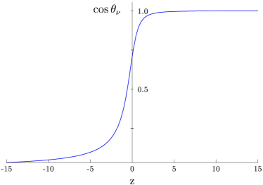
Figure 1: $\cos\theta_{\nu}$ as a function of $z$, see Eq. (54).

We see that $\cos\theta_{\nu}$ varies fast for small $|z|$ and is almost constant for $|z|\gg 0$. Therefore, the least-fine-tuned situations correspond to $|z|\gg 0$ which happens for $|\rho_{3}|\ll\max\{|\rho_{1}|,|\rho_{2}|\}$. Actually, no strong hierarchy is necessary, $\cos\theta_{\nu}$ is very close to 1 for $z$ as small as 3. Note that, if we assume $|\,\vec{e}\,|\,\ll\,|\,\vec{g}\,|$, which is reasonable to assume about all perturbation matrices in order to generate hierarchy between generations, $|\rho_{3}|\ll\max\{|\rho_{1}|,|\rho_{2}|\}$ is satisfied for a huge variety of possible entries $r_{ij}$.

From Eqs. (7), (20) and (53) we see that the most general form of the lepton mixing matrix in this case can be written as :

$$U=\left(\begin{array}[]{ccc}\cos\theta_{e}&\sin\theta_{e}&0\\ -\sin\theta_{e}&\cos\theta_{e}&0\\ 0&0&1\end{array}\right)\left(\begin{array}[]{rrc}\frac{1}{\sqrt{2}}&-\frac{1}{\sqrt{2}}&\ \ \ 0\\ \frac{1}{\sqrt{6}}&\frac{1}{\sqrt{6}}&-\frac{2}{\sqrt{6}}\\ \frac{1}{\sqrt{3}}&\frac{1}{\sqrt{3}}&\ \ \frac{1}{\sqrt{3}}\end{array}\right)\left(\begin{array}[]{ccc}1&0&0\\ 0&\cos\theta_{\nu}&\sin\theta_{\nu}\\ 0&-\sin\theta_{\nu}&\cos\theta_{\nu}\end{array}\right),$$ (56)

where the permutation matrix from Eq. (53) was absorbed in the redefinition of $\cos\theta_{e}$ since the permutation matrix switches columns of the second matrix above and this can be accounted for by rotation of the first two rows of that matrix.

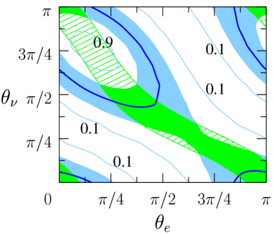
Figure 2: Contours of constant $\sin^{2}\theta_{23}$ (blue) as a function of $\theta_{e}$ and $\theta_{\nu}$. Dark blue contours represent the central value and the blue shaded area corresponds to the $3\sigma$ allowed region. Overlayed is the $3\sigma$ region of $\sin^{2}\theta_{13}$ (green stripes). The green shaded area represents the overlap of $3\sigma$ allowed regions of $\sin^{2}\theta_{23}$ and $\sin^{2}\theta_{13}$.

The lepton mixing matrix in this simplest scheme is given in terms of two parameters $\theta_{e}$ and $\theta_{\nu}$, and so it is not trivial that the resulting three mixing angles can be simultaneously within experimental bounds, although, from the suggestive form of the matrix in the middle of Eq. (56), it might be guessed that it will happen for small $\theta_{e}$ and $\theta_{\nu}$. In Fig. 2 we present contours of constant $\sin^{2}\theta_{23}$ (blue) as a function of $\theta_{e}$ and $\theta_{\nu}$. Dark blue contours represent the central value (Eq. (45)) and the blue shaded area corresponds to the $3\sigma$ allowed region (Eq. (47)). Green stripes represent the $3\sigma$ allowed region of $\sin^{2}\theta_{13}$ given in Eq. (48) and the green area is the overlap of $3\sigma$ allowed regions of $\sin^{2}\theta_{23}$ and $\sin^{2}\theta_{13}$. We see that it is not particularly difficult to achieve a very small $\theta_{13}$ and close to maximal $\theta_{23}$. In the majority of cases, the value of $\sin^{2}\theta_{23}$ consistent with the limits on $\sin^{2}\theta_{13}$ is within or above the $3\sigma$ allowed region.

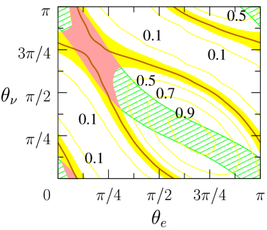
Figure 3: Contours of constant $\sin^{2}\theta_{12}$ (yellow) as a function of $\theta_{e}$ and $\theta_{\nu}$. Brown contours represent the central value and the yellow shaded area corresponds to the $3\sigma$ allowed region. Overlayed is the $3\sigma$ region of $\sin^{2}\theta_{13}$ (green stripes). The pink shaded area represents the overlap of $3\sigma$ allowed regions of $\sin^{2}\theta_{12}$ and $\sin^{2}\theta_{13}$.

In Fig. 3 we present a similar plot for the solar mixing angle. Contours of constant $\sin^{2}\theta_{12}$ are represented by yellow. Brown contours correspond to the central value (Eq. (44)) and the yellow shaded area represents the $3\sigma$ allowed region (Eq. (46)). Green stripes have the same meaning as in the Fig. 2 and the overlap of $3\sigma$ allowed regions of $\sin^{2}\theta_{12}$ and $\sin^{2}\theta_{13}$ is given by the pink area. The value of $\sin^{2}\theta_{12}$ consistent with the limits on $\sin^{2}\theta_{13}$ is always within or above the $3\sigma$ allowed region.

However, the $3\sigma$ allowed regions of all three mixing angles overlap only in two small regions as can be seen in Fig. 4.

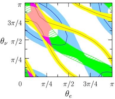
Figure 4: The $3\sigma$ allowed regions of $\sin^{2}\theta_{23}$ (blue, green)), $\sin^{2}\theta_{12}$ (yellow, pink) and $\sin^{2}\theta_{13}$ (green, pink) from Fig. 2 and Fig. 3 overlayed. The magenta regions represent their overlap.

These regions are represented by magenta (note the periodicity of the picture; regions disconnected at the boundaries of the plot are not counted separately).

IV.3 How small can $\sin^{2}\theta_{13}$ be?

Since we do not measure $\theta_{13}$, it is interesting to ask what values of $\sin^{2}\theta_{13}$ can be achieved within this approach while satisfying the $3\sigma$ experimental bounds of $\sin^{2}\theta_{23}$ and $\sin^{2}\theta_{12}$. In Fig. 4 we see that the $3\sigma$ regions of $\sin^{2}\theta_{23}$ and $\sin^{2}\theta_{12}$ overlap in 4 places: two regions containing magenta areas (Region I), and the regions around points $\theta_{e}\simeq\pi/2$, $\theta_{\nu}\simeq 5\pi/8$ and $\theta_{e}\simeq 7\pi/8$, $\theta_{\nu}\simeq 7\pi/8$ (Region II). Note that the two areas in the Region I predict $\sin\theta_{13}$ with opposite signs, and the same applies to the Region II. The predicted values of $\sin^{2}\theta_{13}$ from these regions are:

$$0.008\leq \sin^{2}\theta_{13} \leq 0.14\quad\quad{\rm(Region\;I)},$$ (57)

$$0.22\leq \sin^{2}\theta_{13} \leq 0.66\quad\quad{\rm(Region\;II)}.$$ (58)

Region I overlaps with the experimentally allowed region and it shows that the value of $\sin^{2}\theta_{13}$ which can be accommodated in this approach can be as low as 0.008. Note that this minimal value of $\sin^{2}\theta_{13}$ corresponds to the maximal allowed values of $\sin^{2}\theta_{23}$ and $\sin^{2}\theta_{12}$. On the other hand, the central values of $\sin^{2}\theta_{23}$ and $\sin^{2}\theta_{12}$ correspond to $\sin^{2}\theta_{13}$ near its present experimental upper bound.

IV.4 Consequences for models

The magenta regions in Fig. 4 are not large. Nevertheless, the good news is that they are located around $\theta_{\nu}\simeq\pi/2$ or $\theta_{\nu}\simeq 0,\pi$, which corresponds to the least-fine-tuned possibilities discussed after Eq. (55).

The only allowed values of $\theta_{e}$ are close to $0$ or $\pi/4$. The charged lepton diagonalization matrix corresponding to these two possibilities is close to the forms:

$$U_{e}=\left(\begin{array}[]{rrc}\frac{1}{\sqrt{2}}&-\frac{1}{\sqrt{2}}&\ \ \ 0\\ \frac{1}{\sqrt{6}}&\frac{1}{\sqrt{6}}&-\frac{2}{\sqrt{6}}\\ \frac{1}{\sqrt{3}}&\frac{1}{\sqrt{3}}&\ \ \frac{1}{\sqrt{3}}\end{array}\right)$$ (59)

for $\theta_{e}=0$, and

$$U_{e}=\frac{1}{2\sqrt{3}}\,\left(\begin{array}[]{ccc}-\sqrt{3}-1&\ \ \sqrt{3}-1&\ \ 2\\ \ \ \sqrt{3}-1&-\sqrt{3}-1&\ \ 2\\ \ \ 2&\ \ 2&\ \ 2\end{array}\right)$$ (60)

for $\theta_{e}=\pi/4$ (up to overall sign changes in the rows). The first solution is obvious, since $U_{e}$ is very close to the observed lepton mixing matrix in this case. The second solution is not so obvious and its symmetric form is quite surprising.

Perhaps the simplest models of this kind are those with a dominant 3-3 component in all perturbation matrices, ${\cal E}\simeq{\cal R}\simeq{\rm diag}(0,0,\epsilon)$. This perturbation generates masses of the second family. In this case $U_{e}$ is very close to the one in Eq. (59) and $\vec{g}\simeq(0,0,1)^{T}$. There are many ways to introduce masses of the first family. Simple examples are ${\cal E}\simeq{\cal R}\simeq{\rm diag}(0,\delta,\epsilon)$ (this perturbation was suggested in branco_efd ) or ${\rm diag}(\delta,0,\epsilon)$, where $\delta\ll\epsilon$ (with different numerical values for different perturbation matrices). These situations have all the desired features: $\vec{e}\perp\vec{g}$ (approximately) and $|z|\gg 0$.

It is certainly remarkable that very simple forms of perturbation matrices, which on top of everything can be chosen to be the same for all mass matrices, lead to the observed pattern of fermion masses and mixing. This should come with a warning, however. The simple form of perturbation matrices does not guarantee that it is easy to obtain them naturally in some models. Especially in models with family symmetries this is very complicated compared to the situation in hierarchical models. The reason is that in hierarchical models hierarchy is achieved by suppressing or forbidding some entries in mass matrices. This can be easily achieved by assigning different charges under a family symmetry to different particles. In democratic models however, family symmetries have to allow all entries in mass matrices and yet they have to account for small differences in specific elements of mass matrices. This is certainly not trivial to achieve.

IV.5 Mass of the lightest neutrino

The mass of the lightest neutrino is lifted when the second term in Eq. (32) is taken into account. Since we assume it is just a small correction to the first term, it can be treated as a perturbation. Adding this perturbation does not significantly affect the two heavy eigenvalues and the diagonalization matrix, but it is crucial for the lightest eigenvalue which is exactly zero in the limit when this term is ignored. In the case of non-degenerate eigenvalues the correction to eigenvalues $m_{i}$ of a matrix $\cal M$ generated by a matrix $\delta\cal M$ are given as:

$$\delta m_{i}=u_{i}^{T}\,\delta{\cal M}\,u_{i},$$ (61)

where $u_{i}$ are normalized eigenvectors. In our case $\delta{\cal M}=r{\cal I}$ (up to the overall factor in Eq. (32)) and the eigenvector corresponding to the zero eigenvalue is ${\vec{v}}_{0}\simeq(1,0,0)^{T}$. Therefore,

$$m_{\nu_{1}}=\frac{\lambda^{2}_{\nu}v^{2}_{\nu}}{9M_{eff}}r.$$ (62)

Since $M_{eff}\simeq rM_{0}/3$, see Eq. (30), the mass of the lightest neutrino again does not depend on details of a model in the leading order and is given as:

$$m_{\nu_{1}}=\frac{\lambda_{\nu}^{2}v_{\nu}^{2}}{3M_{0}}.$$ (63)

This result is based on our assumption of the minimal amount of mixing coming from the neutrino diagonalization matrix. However, it is possible to make a prediction which does not depend on this assumption.

Let us suppose that we do not know what the eigenvector corresponding to the lightest eigenvalue is. Due to the universal form of $\delta{\cal M}$, we have

$${\vec{v}}_{0}^{\,T}\,\delta{\cal M}\,{\vec{v}}_{0}=r\,\xi^{2},$$ (64)

where

$$\xi=\sum_{i=1}^{3}v_{0i},$$ (65)

and so the mass of the lightest neutrino is given as:

$$m_{\nu_{1}}=\frac{\lambda^{2}_{\nu}v^{2}_{\nu}}{3M_{0}}\,\xi^{2}.$$ (66)

In general $\xi$ can be anything between 0 and $\sqrt{3}$. However, in order to satisfy bounds on lepton mixing angles $\xi$ cannot be arbitrary. The 3-1 element of the lepton mixing matrix is given by:

$$U_{\tau 1}=\left(U_{e}U_{\nu_{L}}^{\dagger}\right)_{31}=\left(\frac{1}{\sqrt{3}},\frac{1}{\sqrt{3}},\frac{1}{\sqrt{3}}\right).{\vec{v}}_{0}=\frac{1}{\sqrt{3}}\xi,$$ (67)

and so

$$m_{\nu_{1}}=\frac{\lambda^{2}_{\nu}v^{2}_{\nu}}{M_{0}}\,U_{\tau 1}^{2}.$$ (68)

Note that the 3rd row in $U_{e}$ is not model dependent unlike the first two rows are! It can receive only small corrections from the perturbation matrix. Finally, in the case of complex matrices, ${\vec{v}}^{\,T}$ in Eq. (64) becomes ${\vec{v}}^{\,{\dagger}}$ and $U_{\tau 1}^{2}$ in Eq. (68) becomes $|\,U_{\tau 1}\,|^{2}$.

Although we do not measure $U_{\tau 1}$, it is related to the observed mixing angles due to the unitarity of the lepton mixing matrix. In the case $\sin\theta_{13}\simeq 0$ it is simply given by

$$U_{\tau 1}=\sin\theta_{23}\,\sin\theta_{12}.$$ (69)

A global analysis of neutrino oscillation data Gonzalez-Garcia:2003 gives the $3\sigma$ range:

$$0.20\leq\,|\,U_{\tau 1}\,|\,\leq 0.58.$$ (70)

The value of $U_{\tau 1}=1/\sqrt{3}$ in which case Eq. (68) gives the same result as Eq. (63) is close to the upper limit.

The masses of the two heavier neutrinos are given in terms of $r_{ij},\,\epsilon_{\nu kl}$, and so they are highly model dependent. Let us look at a simple example to get a feeling for typical values of perturbations which lead to the observed spectrum. Let us assume that the form of all perturbations is $\sim{\rm diag}(\delta,0,\epsilon)$. In this case we have: $|\,\vec{e}\,|^{2}=\delta_{\nu}^{2}$, $|\,\vec{g}\,|^{2}=\epsilon_{\nu}^{2}$, $r_{1}=\epsilon_{r}$, $r_{2}=\delta_{r}$, and $r_{3}=0$, from which we get: $\rho_{1}=\epsilon_{r}\delta_{\nu}^{2}$, $\rho_{2}=\delta_{r}\epsilon_{\nu}^{2}$, $\rho_{3}=0$, and $r=r_{1}r_{2}$. The neutrino masses are given by:

$$m_{\nu_{2,3}}=\frac{\lambda^{2}_{\nu}v^{2}_{\nu}}{9M_{eff}}\,\left\{\rho_{1},\rho_{2}\right\}\simeq\frac{\lambda^{2}_{\nu}v^{2}_{\nu}}{3M_{0}\ r}\,\left\{\rho_{1},\rho_{2}\right\}\simeq\frac{\lambda^{2}_{\nu}v^{2}_{\nu}}{3M_{0}}\,\left\{\frac{\delta_{\nu}^{2}}{\delta_{r}},\frac{\epsilon_{\nu}^{2}}{\epsilon_{r}}\right\}.$$ (71)

Using Eq. (68) we get

$$m_{\nu_{2,3}}\simeq\frac{m_{\nu_{1}}}{3\,|\,U_{\tau 1}\,|^{2}}\,\left\{\frac{\delta_{\nu}^{2}}{\delta_{r}},\frac{\epsilon_{\nu}^{2}}{\epsilon_{r}}\right\}.$$ (72)

In order to have $m_{\nu_{2}},m_{\nu_{3}}>m_{\nu_{1}}$ we need $\delta_{r}<\delta_{\nu}^{2}$ and $\epsilon_{r}<\epsilon_{\nu}^{2}$, and so the hierarchy in the right-handed neutrino mass matrix has to be much larger than the hierarchy in the neutrino Yukawa matrix. This coincides with the assumption we had to make in order to achieve large lepton mixing, see Eq. (32).

In simple SO(10) type models $\lambda_{u}v_{u}=\lambda_{\nu}v_{\nu}$, in which case the lightest and the heaviest fermion of the standard model are connected through the relation in Eq. (68) where $\lambda_{\nu}^{2}v_{\nu}^{2}$ is replaced by $m_{top}^{2}$ (actually, to be precise, $\lambda_{u}=\lambda_{\nu}$ is a relation at the GUT scale and the effects of the renormalization group running between the GUT scale and the electroweak scale should be taken into account). This is a very pleasant feature since we can further identify $M_{0}$ with the GUT scale, $M_{GUT}\sim 2\times 10^{16}$ GeV, in which case we get

$$m_{\nu_{1}}=\frac{m_{top}^{2}}{M_{GUT}}\,|\,U_{\tau 1}\,|^{2},$$ (73)

and predict the mass of the lightest neutrino to be between $5\times 10^{-5}$ eV and $5\times 10^{-4}$ eV depending on the value of $U_{\tau 1}$.

From experimental values of $m_{\nu_{2}}$ and $m_{\nu_{3}}$, given in Eqs. (49) and (50), and from the predicted mass of $m_{\nu_{1}}$, we see that $\epsilon_{\nu}^{2}/\epsilon_{r}$ in Eq. (72) is of order $10^{2}$ and $\delta_{\nu}^{2}/\delta_{r}$ is an order of magnitude smaller. The largest $\epsilon_{f}$ necessary to fit the masses of the second generation of charged fermions corresponds to $\epsilon_{e}\simeq 0.28$. If we take $\epsilon_{\nu}\simeq 0.1$, we find $\epsilon_{r}\simeq 10^{-4}$ and the mass of the second right-handed neutrino is $M_{2}\simeq(10^{-4}-10^{-5})M_{3}$, where $M_{3}=M_{0}=M_{GUT}$. This is a very rough estimate and it is not clear how to reasonably estimate $M_{1}$, besides the relation $M_{1}<M_{2}$. We conclude that the spectrum of the right-handed neutrinos consistent with bi-large mixing in our setup is $M_{1}<M_{2}<10^{-4}M_{3}$ and $M_{3}\simeq M_{GUT}$.

V A Symmetry for Third Generation Dominance

The democratic Yukawa matrices are well motivated by $S_{3L}\times S_{3R}$ family symmetry Fritzsch_Xing_review . However, the right-handed neutrino Majorana mass matrix is then constrained by the $S_{3R}$ symmetry only and the democratic form is not unique. The most general form of the right-handed neutrino mass matrix is given as a linear combination of the democratic matrix and the identity matrix.

It has been shown that the democratic forms of Yukawa matrices and the right-handed neutrino mass matrix are uniquely specified by imposing a $Z_{3}$ symmetry realized in the following way branco_Z3 :

$$f_{Li} \rightarrow P^{\dagger}_{ij}f_{Lj},$$ (74)

$$f_{Ri} \rightarrow P_{ij}f_{Rj},$$ (75)

where

$$P=\frac{i\omega^{*}}{\sqrt{3}}\left(\begin{array}[]{ccc}\omega&1&1\\ 1&\omega&1\\ 1&1&\omega\\ \end{array}\right),\quad\quad\omega=e^{i\frac{2\pi}{3}}.$$ (76)

It is straightforward to check that this is indeed a $Z_{3}$ symmetry, and the proof that it is responsible for the democratic form of Yukawa matrices and the right-handed neutrino mass matrix can be found in Ref. branco_Z3 . Here we provide an alternative proof and a very simple understanding of this peculiar symmetry.

Let us first note that a democratic matrix $M_{D}$ (which represents both Yukawa matrices and the right-handed Majorana mass matrix):

$$M_{D}=\frac{1}{3}\left(\begin{array}[]{ccc}1&1&1\\ 1&1&1\\ 1&1&1\\ \end{array}\right),$$ (77)

can be brought to a diagonal (hierarchical) form:

$$M_{H}=\left(\begin{array}[]{ccc}0&0&0\\ 0&0&0\\ 0&0&1\\ \end{array}\right),$$ (78)

by a unitary transformation

$$M_{H}=U_{\cal I}M_{D}U_{\cal I}^{T},$$ (79)

where $U_{\cal I}$ is given in Eq. (20).

It is obvious that a $Z_{3}$ symmetry under which the first two generations of left-handed fermions have charge -1, the first two generations of right-handed fermions have charge +1 (or, equivalently, charge conjugates of right-handed fermions have charge -1), and the third generation of fermions has charge zero uniquely specifies the $M_{H}$ form of Yukawa matrices and the right-handed neutrino Majorana mass matrix. It follows from the fact that any coupling involving first and/or second generation fermions is simply forbidden. Therefore the only non-zero element of a mass matrix is the 3-3 element. This can be written in the form of transformations (74) and (75) with $P$ replaced by $P_{H}$:

$$P_{H}=\left(\begin{array}[]{ccc}\omega&0&0\\ 0&\omega&0\\ 0&0&1\\ \end{array}\right),$$ (80)

where the subscript H indicates that it is a symmetry transformation specifying the hierarchical form of mass matrices. Therefore we proved:

$$P_{H}MP_{H}=M\quad\Leftrightarrow\quad M=\lambda M_{H}.$$ (81)

Now we can rotate this result to the democratic basis:

$$U_{\cal I}^{T}P_{H}U_{\cal I}U_{\cal I}^{T}MU_{\cal I}U_{\cal I}^{T}P_{H}U_{\cal I}=U_{\cal I}^{T}MU_{\cal I}\quad\Leftrightarrow\quad U_{\cal I}^{T}MU_{\cal I}=\lambda U_{\cal I}^{T}M_{H}U_{\cal I},$$ (82)

and we obtain:

$$PM^{\prime}P=M^{\prime}\quad\Leftrightarrow\quad M^{\prime}=\lambda M_{D},$$ (83)

where $M^{\prime}=U_{\cal I}^{T}MU_{\cal I}$ and

$$P=U_{\cal I}^{T}P_{H}U_{\cal I}.$$ (84)

Inserting $P_{H}$ from Eq. (80) and $U_{\cal I}$ from Eq. (20) it is straightforward to find that the form of the transformation matrix $P$ which guarantees the democratic form of all mass matrices is exactly that of Eq. (76).

We see that the special form of $P$ in Eq. (76) is just a simple $Z_{3}$ symmetry which allows only 3-3 elements in mass matrices rotated into the democratic basis. This shows that the approach in which the right-handed neutrino Majorana mass matrix and Yukawa matrices have in the leading order democratic form is equivalent to the hierarchical approach in which the 3-3 elements in Yukawa matrices and the right-handed neutrino mass matrix dominate. The results obtained in previous sections can be translated into results in corresponding hierarchical models . Namely, the prediction for the mass of the lightest neutrino does not change, since mass eigenstates are not basis dependent. The necessary (and basis independent) requirement for achieving large mixing in this scheme is $M_{1},M_{2}<10^{-4}M_{3}$, i.e., the third generation right-handed neutrino has to dominate even more than the third generation of quarks and charged leptons. Thus third generation dominance is a suitable name for this scenario.

Besides this $Z_{3}$ symmetry, the democratic mass matrices have also larger symmetries, like $S_{3}$, for example, which can be used to specify perturbation matrices in the process of family symmetry breaking and thus distinguish between hierarchical and democratic starting point . However, the complicated form of the $Z_{3}$ symmetry in the democratic basis compared to the simple form in the hierarchical basis further amplifies the difficulties in constructing specific models as discussed at the end of Sec. IV.4.

The fact that these mass matrices are motivated by a simple $Z_{3}$ symmetry is certainly a very pleasant feature. Unlike $S_{3L}\times S_{3R}$, this $Z_{3}$ symmetry acts in the same way on all particles in each generation. Therefore this approach can be readily embedded into GUT models, like SO(10).

VI Conclusions

We showed that both small mixing in the quark sector and large mixing in the lepton sector can be obtained from a simple assumption of universality of Yukawa couplings and the right-handed neutrino Majorana mass matrix in the leading order. We discussed conditions under which bi-large mixing in the lepton sector is achieved with a minimal amount of fine-tuning requirements for possible models. From knowledge of the solar and atmospheric mixing angles we determined the allowed values of $\sin\theta_{13}$. The central values of $\sin^{2}\theta_{23}$ and $\sin^{2}\theta_{12}$ predict $\sin^{2}\theta_{13}$ near its present experimental upper bound, while it can be as small as 0.008 if both $\sin^{2}\theta_{23}$ and $\sin^{2}\theta_{12}$ are near their $3\sigma$ upper bounds.

We showed that this approach is equivalent to the hierarchical approach in which the 3-3 elements in Yukawa matrices and the right-handed neutrino mass matrix dominate. The necessary (and basis independent) requirement for achieving large mixing in this scheme is $M_{1},M_{2}<10^{-4}M_{3}$. This is phenomenologically very interesting because it was found that under these conditions the effective Majorana mass in neutrinoless double beta decay might be related to the CP violating phase controlling leptogenesis Pascoli:2003uh . Furthermore, since the heaviest right-handed neutrino effectively decouple, this scenario might provide a natural framework for models with two right-handed neutrinos only Frampton:2002qc ; Raidal:2002xf ; Raby:2003ay .

The virtue of this approach is that all mass matrices are treated in the same way, providing a simple framework which can be easily embedded into GUTs. If embedded into simple GUTs, the third generation Yukawa coupling unification (at least approximate) is inevitable which is theoretically very appealing and it has interesting consequences for phenomenology yukawa . Note that in this framework it is achieved without making one generation different from others at a fundamental level. On the other hand, the spectrum of the first two generations of quarks and charged leptons crucially depends on small perturbations. In the neutrino sector, the heavier two neutrinos are model dependent, while the mass of the lightest neutrino in this approach does not depend on perturbations in the leading order. The right-handed neutrino mass scale can be identified with the GUT scale, in which case the mass of the lightest neutrino is given as $(m_{top}^{2}/M_{GUT})\sin^{2}\theta_{23}\sin^{2}\theta_{12}$ in the limit $\sin\theta_{13}\simeq 0$.

We do not provide any understanding of the origin of universal mass matrices and their perturbations. It is not straightforward to construct such models with family symmetries. Nevertheless, it is worthwhile to look for alternatives: extra dimensions or composite models. No matter what the origin is, having all three generations indistinguishable in leading order is certainly something one would like to see in the fundamental theory. After all, the three generations have exactly the same quantum numbers in the standard model and even in simple GUT models. Why should their Yukawa couplings be so different?

- (1) for a review, see H. Fritzsch and Z. Xing, Prog. Part. Nucl. Phys. 45, 1 (2000).
- (2) for recent reviews, see S. F. King, arXiv:hep-ph/0310204; A. Y. Smirnov, arXiv:hep-ph/0311259.
- (3) L. Hall, H. Murayama and N. Weiner, Phys. Rev. Lett. 84, 2572 (2000).
- (4) H. Harari, H. Haut and J. Weyers, Phys. Lett. B78, 459 (1978); Y. Koide, Phys. Rev. D39, 1391 (1989);
- (5) H. Fritzsch and Z. Xing, Phys. Lett. B372, 265 (1996); M. Fukugita, M. Tanimoto and T. Yanagida Phys. Rev. D57, 4429 (1998).
- (6) R. N. Mohapatra and S. Nussinov, Phys. Lett. B441, 299 (1998).
- (7) R. Dermisek, arXiv:hep-ph/0312206v1.
- (8) E. Kh. Akhmedov, G.C. Branco, F.R. Joaquim and J.I. Silva-Marcos, Phys. Lett. B498, 237 (2001);
- (9) G.C. Branco and J.I. Silva-Marcos, Phys. Lett. B526, 104 (2002).
- (10) T. Teshima and T. Asai, Prog. Theor. Phys. 105, 763 (2001); T. Teshima, T. Asai and Y. Abe, Phys. Rev. D66, 093011 (2002).
- (11) M. Gell-Mann, P. Ramond and R. Slansky, in Supergravity, ed. P. van Nieuwenhuizen and D.Z. Freedman, North-Holland, Amsterdam, 1979, p. 315; T. Yanagida, in Proceedings of the Workshop on the unified theory and the baryon number of the universe, ed. O. Sawada and A. Sugamoto, KEK report No. 79-18, Tsukuba, Japan, 1979; R. N. Mohapatra and G. Senjanovic, Phys. Rev. Lett. 44, 912 (1980).
- (12) M. C. Gonzalez-Garcia and C. Pena-Garay, Phys. Rev. D 68, 093003 (2003);
- (13) M. Maltoni, T. Schwetz, M. A. Tortola and J. W. F. Valle, Phys. Rev. D 68, 113010 (2003).
- (14) R. Dermisek, arXiv:hep-ph/0406017.
- (15) R. Dermisek, arXiv:hep-ph/0409195.
- (16) S. Pascoli, S. T. Petcov and W. Rodejohann, Phys. Rev. D 68, 093007 (2003) [arXiv:hep-ph/0302054]. However, see also W. Rodejohann, Eur. Phys. J. C 32, 235 (2004).
- (17) P. H. Frampton, S. L. Glashow and T. Yanagida, Phys. Lett. B 548, 119 (2002) [arXiv:hep-ph/0208157].
- (18) M. Raidal and A. Strumia, Phys. Lett. B 553, 72 (2003) [arXiv:hep-ph/0210021].
- (19) S. Raby, Phys. Lett. B 561, 119 (2003) [arXiv:hep-ph/0302027].
- (20) See for example recent studies, T. Blazek, R. Dermisek and S. Raby, Phys. Rev. Lett. 88, 111804 (2002); ibid Phys. Rev. D65, 115004 (2002); K. Tobe and J. D. Wells, Nucl. Phys. B 663, 123 (2003); D. Auto, H. Baer, C. Balazs, A. Belyaev, J. Ferrandis and X. Tata, JHEP 0306, 023 (2003); R. Dermisek, S. Raby, L. Roszkowski and R. Ruiz De Austri, JHEP 0304, 037 (2003); S. Komine and M. Yamaguchi, Phys. Rev. D 65, 075013 (2002); U. Chattopadhyay, A. Corsetti and P. Nath, Phys. Rev. D66, 035003 (2002); S. Profumo, Phys. Rev. D 68, 015006 (2003); C. Balazs and R. Dermisek, JHEP 0306, 024 (2003); C. Pallis, Nucl. Phys. B 678, 398 (2004); and references therein.