IFIC/03$-$38

FTUV/03$-$1215

$\tau\to\pi\pi\pi\nu_{\tau}$ decays in the Resonance Effective Theory

D. Gómez Dumm^a, A. Pich^b, J. Portolés^b

^a IFLP, Depto. de Física, Universidad Nacional de La Plata,
C.C. 67, 1900 La Plata, Argentina
 
^bDepartament de Física Teòrica, IFIC, CSIC – Universitat de València
Apt. Correus 22085, E-46071 València, Spain

$\tau\to\pi\pi\pi\nu_{\tau}$ decays are analysed within the framework of the resonance effective theory of QCD. We work out the relevant Lagrangian that describes the axial–vector current hadronization contributing to these processes, in particular the local $a_{1}$(1260)–$\rho$(770)–Goldstone interactions. The new coupling constants are constrained by imposing the asymptotic behaviour of the corresponding spectral function within QCD. Hence we compare the theoretical framework with the experimental data, obtaining a good quality fit from the ALEPH spectral function and branching ratio. We also get values for the mass and on–shell width of the $a_{1}$(1260) resonance. In this way we are able to provide the structure functions that have been measured by OPAL and CLEO-II and we find an excellent agreement.

PACS : 11.30.Rd, 11.40.-q, 13.35.-r, 14.60.Fg
      Keywords : Hadronic tau decays, effective theories, QCD

1 Introduction

The decays of the $\tau$ lepton offer an excellent laboratory for the analysis of various topics in particle physics. In particular, $\tau$ decays into hadrons allow to study the properties of the vector and axial–vector QCD currents, and provide relevant information on the dynamics of the resonances entering into the processes. The hadronization of those currents involves the strong interaction at low energies and, therefore, non–perturbative features of QCD have to be implemented properly into their evaluation. The Effective Theory framework has a long–history of successful achievements in this task.

At very low energies, typically $E\ll M_{\rho}$ (being $M_{\rho}$ the mass of the $\rho$(770), the lightest hadron resonance), chiral perturbation theory ($\chi$PT) [1, 2] is the corresponding effective theory of QCD. However the decays $\tau\to\pi\pi\pi\nu_{\tau}$, through their full energy spectrum, happen to be driven by the $\rho$(770) and $a_{1}$(1260) resonances, mainly, in an energy region where they reach their on–shell peaks. In consequence $\chi$PT is not directly applicable to the study of the whole spectrum but only to the very low energy domain [3]. Until now the standard way of dealing with these decays has been to use ${\cal O}(p^{2})$ $\chi$PT to fix the normalization of the amplitudes in the low energy region and, accordingly, to include the effects of vector and axial–vector meson resonances by modulating the amplitudes with ad hoc Breit–Wigner functions [4, 5]. However we will see that this modelization is not consistent with ${\cal O}(p^{4})$ $\chi$PT, a fact that could potentially spoil any outcome provided by this procedure.

In the last years several experiments have collected good quality data on $\tau\to\pi\pi\pi\nu_{\tau}$, such as branching ratios and spectra [6, 7] or structure functions [8], and their analysis within a model–independent framework is highly desirable if one wishes to collect information on the hadronization of the QCD currents. The Effective Field Theory still provides the proper tool to proceed in this study. At energies $E\sim M_{\rho}$ the resonance mesons are active degrees of freedom that cannot be integrated out, as in $\chi$PT, and they have to be properly included into the relevant Lagrangian [9]. The procedure is ruled by the chiral symmetry under $SU(3)_{\mathrm{L}}\otimes SU(3)_{\mathrm{R}}$, that drives the interaction of Goldstone bosons (the lightest octet of pseudoscalar mesons), and the $SU(3)_{\mathrm{V}}$ assignments of the resonance multiplets. Its systematic arrangement has been put forward in Refs. [10, 11] as the Resonance Chiral Theory (R$\chi$T). We will attach to this framework and we will complete it, when needed, in order to fulfill our requirements.

A complementary tool, thoroughly intertwined with the R$\chi$T, is the large number of colours ($N_{C}$) limit of QCD. Strong interactions in the resonance region lack an expansion parameter that, as in $\chi$PT, could provide a perturbative treatment of the amplitudes. However it has been pointed out [12] that the inverse of the number of colours of the gauge group $SU(N_{C})$ could accomplish this task. Indeed large–$N_{C}$ QCD shows features that resemble, both qualitatively and quantitatively, the $N_{C}=3$ case [13]. Relevant consequences of this approach are that meson dynamics in the large–$N_{C}$ limit is described by the tree diagrams of an effective local Lagrangian; moreover, at the leading order, one has to include the contributions of the infinite number of zero–width resonances that constitute the spectrum of the theory.

In this article we study the $\tau\to\pi\pi\pi\nu_{\tau}$ processes within the Resonance Effective Theory of QCD. We will evaluate the form factor associated to the $J^{P}=1^{+}$ piece of the axial–vector current that is, by far, the dominant contribution to these processes. To proceed we will work out the effective Lagrangian that endows the dynamics of the decay at the leading order in the $1/N_{C}$ expansion, though we will consider the lightest vector and axial–vector octets of resonances only. Moreover we will provide these with a finite width, due to the fact that they do really resonate along the full energy spectrum. In order to improve the construction of the Effective Theory we will constrain the new unknown couplings in the Lagrangian by demanding the asymptotic behaviour of the form factor ruled by perturbative QCD. The theoretical construction will be followed by the phenomenological analysis of experimental data.

The article is organized as follows : The resonance effective theory is studied in Sect. 2. In Sect. 3 we consider the $\tau\to\pi\pi\pi\nu_{\tau}$ processes and calculate, within our approach, the relevant hadronic matrix elements. Sect. 4 is devoted to discuss the constraints imposed by perturbative QCD on the form factors driven by the resonances, which lead to a set of relations between the coupling constants. The analysis of experimental data within our framework is presented in Sect. 5, while in Sect. 6 we sketch our conclusions. An Appendix recalls the basic features of the very–low energy domain of the $\tau^{-}\to\pi^{+}\pi^{-}\pi^{-}\nu_{\tau}$ process within $\chi$PT.

2 The Resonance Effective Theory of QCD

The very low–energy strong interaction in the light quark sector is known to be ruled by the $SU(3)_{\mathrm{L}}\otimes SU(3)_{\mathrm{R}}$ chiral symmetry of massless QCD implemented in $\chi$PT. The leading ${\cal O}(p^{2})$ Lagrangian is :

$${\cal L}_{\chi}^{(2)}=\frac{F^{2}}{4}\langle u_{\mu}u^{\mu}+\chi_{+}\rangle\ ,$$ (1)

where

$$u_{\mu} = i[u^{\dagger}(\partial_{\mu}-ir_{\mu})u-u(\partial_{\mu}-i\ell_{\mu})u^{\dagger}]\ ,$$

$$\chi_{\pm} = u^{\dagger}\chi u^{\dagger}\pm u\chi^{\dagger}u\ \ \ \ ,\ \ \ \ \chi=2B_{0}(s+ip)\;\;,$$ (2)

and $\langle\ldots\rangle$ is short for a trace in the flavour space. The Goldstone octet of pseudoscalar fields

$$\Phi(x)\equiv\,\frac{\displaystyle 1}{\displaystyle\sqrt{2}}\,\sum_{a=1}^{8}\,\lambda_{a}\,\varphi_{a}\,=\,\pmatrix{{1\over\sqrt{2}}\pi^{0}\,+\,{1\over\sqrt{6}}\eta_{8}&\pi^{+}&K^{+}\cr\pi^{-}&-{1\over\sqrt{2}}\pi^{0}\,+\,{1\over\sqrt{6}}\eta_{8}&K^{0}\cr K^{-}&\bar{K}^{0}&-{2\over\sqrt{6}}\eta_{8}}$$ (3)

is realized non–linearly into the unitary matrix in the flavour space

$$u(\varphi)=\exp\left\{i\frac{\Phi}{\sqrt{2}\,F}\right\}\;\;\;,$$ (4)

that transforms as

$$u(\varphi)\to g_{R}\,u(\varphi)\,h(g,\varphi)^{\dagger}=h(g,\varphi)\,u(\varphi)\,g_{L}^{\dagger}\;\;,$$ (5)

with $g\equiv(g_{L},g_{R})\,\in\,SU(3)_{\mathrm{L}}\otimes SU(3)_{\mathrm{R}}$ and $h(g,\varphi)\,\in\,SU(3)_{V}$. External hermitian matrix fields $r_{\mu}$, $\ell_{\mu}$, $s$ and $p$ promote the global $SU(3)_{\mathrm{L}}\otimes SU(3)_{\mathrm{R}}$ symmetry to a local one. Interactions with electroweak bosons can be accommodated through the vector $v_{\mu}=(r_{\mu}+\ell_{\mu})/2$ and axial–vector $a_{\mu}=(r_{\mu}-\ell_{\mu})/2$ fields. The scalar field $s$ incorporates explicit chiral symmetry breaking through the quark masses $s={\cal M}\,+\ldots$, with ${\cal M}=\mathrm{diag}(m_{u},m_{d},m_{s})$ and, finally, $F\simeq F_{\pi}\simeq 92.4\,\mbox{MeV}$ is the pion decay constant and $B_{0}F^{2}=-\langle 0|\bar{\psi}\psi|0\rangle_{0}$ in the chiral limit.

The final hadron system in the $\tau\to\pi\pi\pi\nu_{\tau}$ decays spans a wide energy region $3m_{\pi}\stackrel{{\scriptstyle<}}{{{}_{\sim}}}E\stackrel{{\scriptstyle<}}{{{}_{\sim}}}M_{\tau}$ that is populated by resonances. As a consequence an effective theory description of the full energy spectrum requires to include the resonances as active degrees of freedom and, therefore, to consider R$\chi$T. This recalls the ideas of effective Lagrangians from Ref. [9]. The interaction of the Goldstone bosons (the lightest octet of pseudoscalar mesons) with the resonances is driven by chiral symmetry, while the resonances enter as $SU(3)_{\mathrm{V}}$ multiplets. In Ref. [10] the simplest couplings were introduced using the antisymmetric tensor formulation to describe the vector and axial–vector resonances but keeping linear terms in the latter, i.e. allowing for the couplings of the pseudoscalars to only one resonance. This formalism proved successful in accounting, upon integration of resonances, for the bulk of the low–energy coupling constants at ${\cal O}(p^{4})$ in $\chi$PT with no need of the addition of local terms [11]. We will attach to this antisymmetric tensor formulation and, accordingly, we will not include the ${\cal O}(p^{4})$ $\chi$PT couplings into our effective action in order to avoid double counting of contributions. The success of R$\chi$T in the description of many observables has been remarkable, in particular for the pion electromagnetic form factor entering $\tau^{-}\to\pi^{-}\pi^{0}\nu_{\tau}$ [14].

Therefore in order to introduce the octet of resonance fields we define [10]

$$R\equiv\frac{1}{\sqrt{2}}\sum_{a=1}^{8}\lambda_{a}R_{a}\;,$$ (6)

where $R_{a}=V_{a},A_{a}$, stands for vector and axial–vector meson fields, respectively, that transform as

$$R \to h(g,\varphi)\,R\,h(g,\varphi)^{\dagger}$$ (7)

under the chiral group. The flavour structure of the resonances is analogous to the Goldstone bosons in Eq. (3). We also introduce the covariant derivative

$$\nabla_{\mu}X \equiv \partial_{\mu}X+[\Gamma_{\mu},X]\;\;,$$ (8)

$$\Gamma_{\mu} = \frac{\displaystyle 1}{\displaystyle 2}\,[\,u^{\dagger}(\partial_{\mu}-ir_{\mu})u+u(\partial_{\mu}-i\ell_{\mu})u^{\dagger}\,]\;\;,$$

for any object $X$ that transforms as $R$ in Eq. (7), like $u_{\mu}$ and $\chi_{\pm}$.

Let us now restrict the analysis to the case of $V(1^{--})$ and $A(1^{++})$ resonances, in order to describe the couplings of $\rho$(770) and $a_{1}$(1260) states, respectively. Moreover we include the lightest $SU(3)_{\mathrm{V}}$ octet of both vector and axial–vector resonances only. Although the leading $1/N_{C}$ expansion requires to consider an infinite number of resonances their contribution happens to be suppressed as their masses become heavier.

The kinetic terms for the spin 1 resonances in the Lagrangian read, in the antisymmetric tensor formulation,

$${\cal L}_{\rm kin}^{R}=-\frac{1}{2}\langle\nabla^{\lambda}R_{\lambda\mu}\nabla_{\nu}R^{\nu\mu}-\frac{M_{R}^{2}}{2}R_{\mu\nu}R^{\mu\nu}\rangle\;\;\;,\;\;\;\;\;R\,=\,V,A\;,$$ (9)

being $M_{V}$, $M_{A}$ the mass of the octet of vector and axial–vector resonances, respectively. The lowest order interaction Lagrangian includes three coupling constants [10],

$${\cal L}_{2}^{\rm V} = \frac{F_{V}}{2\sqrt{2}}\langle V_{\mu\nu}f_{+}^{\mu\nu}\rangle+i\,\frac{G_{V}}{\sqrt{2}}\langle V_{\mu\nu}u^{\mu}u^{\nu}\rangle\;\,,$$

$${\cal L}_{2}^{\rm A} = \frac{F_{A}}{2\sqrt{2}}\langle A_{\mu\nu}f_{-}^{\mu\nu}\rangle\;,$$ (10)

where $f_{\pm}^{\mu\nu}=uF_{L}^{\mu\nu}u^{\dagger}\pm u^{\dagger}F_{R}^{\mu\nu}u$ and $F_{R,L}$ are the field strength tensors associated with the external right and left fields. All coupling parameters $F_{V}$, $G_{V}$ and $F_{A}$ are real. Notice that the ${\cal O}(p^{2})$ interaction Lagrangian (2) does not allow a tree-level coupling of the form $a_{1}(1260)\pi\pi\pi$.

In the case of $\tau\to\pi\pi\pi\nu_{\tau}$, in addition to one–resonance–exchange diagrams one has to consider the contribution given by the chain $a_{1}(1260)\to\rho(770)\pi\to\pi\pi\pi$, which is mediated by both vector and axial–vector resonances. Thus we need to go one step beyond the analysis in Ref. [10], including bilinear terms in the resonance fields that lead to a coupling of the form $a_{1}\rho\pi$. For the processes under study, we only need to consider terms that include a vertex with one pseudoscalar. This goal is achieved with one ${\cal O}(p^{2})$ chiral tensor. Hence the most general interaction Lagrangian allowed by the symmetry constraints can be written as

$${\cal L}_{2}^{\rm VAP}\,=\,\sum_{i=1}^{5}\,\lambda_{i}\,{\cal O}^{i}_{\rm VAP}\;\;,$$ (11)

where $\lambda_{i}$ are new unknown real adimensional couplings, and the operators ${\cal O}^{i}_{\rm VAP}$ are given by

$${\cal O}^{1}_{\rm VAP} = \langle\,[\,V^{\mu\nu}\,,\,A_{\mu\nu}\,]\,\chi_{-}\,\rangle\;\;,$$

$${\cal O}^{2}_{\rm VAP} = i\,\langle\,[\,V^{\mu\nu}\,,\,A_{\nu\alpha}\,]\,h_{\mu}^{\;\alpha}\,\rangle\;\;,$$ (12)

$${\cal O}^{3}_{\rm VAP} = i\,\langle\,[\,\nabla^{\mu}V_{\mu\nu}\,,\,A^{\nu\alpha}\,]\,u_{\alpha}\,\rangle\;\;,$$

$${\cal O}^{4}_{\rm VAP} = i\,\langle\,[\,\nabla^{\alpha}V_{\mu\nu}\,,\,A_{\alpha}^{\;\nu}\,]\,u^{\mu}\,\rangle\;\;,$$

$${\cal O}^{5}_{\rm VAP} = i\,\langle\,[\,\nabla^{\alpha}V_{\mu\nu}\,,\,A^{\mu\nu}\,]\,u_{\alpha}\,\rangle\;\;,$$

with $h_{\mu\nu}=\nabla_{\mu}u_{\nu}+\nabla_{\nu}u_{\mu}$. We emphasize that this set is a complete basis for constructing vertices with only one pseudoscalar; for a larger number of pseudoscalars additional operators may emerge. As we are only interested in tree level diagrams, the equation of motion arising from ${\cal O}(p^{2})$ $\chi$PT,

$$h_{\alpha}^{\;\alpha}\,=\,i\,\chi_{-}\,-\,\frac{\displaystyle i}{\displaystyle 3}\langle\chi_{-}\rangle\;,$$ (13)

has been used in ${\cal L}_{2}^{\rm VAP}$ in order to eliminate one of the possible operators.

In summary we will proceed in the following by considering the relevant Resonance Chiral Theory given by :

$${\cal L}_{\rm R\chi T}\,=\,{\cal L}_{\chi}^{(2)}\,+\,{\cal L}_{\rm kin}^{\rm V}\,+\,{\cal L}_{\rm kin}^{\rm A}\,+\,{\cal L}_{2}^{\rm V}\,+\,{\cal L}_{2}^{\rm A}\,+\,{\cal L}_{2}^{\rm VAP}\;\;.$$ (14)

It is important to notice that ${\cal L}_{\rm R\chi T}$ is not an effective theory of QCD for arbitrary couplings in the interaction terms ${\cal L}_{2}^{\rm V/A}$ and ${\cal L}_{2}^{\rm VAP}$. These carry some symmetry properties of QCD, implemented in the operators, that do not give any information on the coupling constants. However we will see in Section 4 that well accepted dynamical properties of the underlying theory provide some information on those couplings. This is as far as we can go without including modelizations.

3 Axial–vector current form factors in $\tau\to\pi\pi\pi\nu_{\tau}$

In this Section we describe the $\tau\to\pi\pi\pi\nu_{\tau}$ decays in the isospin limit and proceed to calculate the relevant hadronic matrix element within the resonance effective theory given by ${\cal L}_{\rm R\chi T}$. The decay amplitude for the $\tau^{-}\to\pi^{+}\pi^{-}\pi^{-}\nu_{\tau}$ and $\tau^{-}\to\pi^{-}\pi^{0}\pi^{0}\nu_{\tau}$ processes can be written as

$${\cal M}_{\pm}\;=\;-\,\frac{G_{F}}{\sqrt{2}}\,V_{ud}\,\bar{u}_{\nu_{\tau}}\gamma^{\mu}\,(1-\gamma_{5})u_{\tau}\,T_{\pm\mu}\;\;,$$ (15)

where $V_{ud}$ is an element of the Kobayashi–Maskawa matrix and $T_{\pm\mu}$ is the hadronic matrix element of the participating $V_{\mu}-A_{\mu}$ QCD currents. In the isospin limit there is no contribution of the vector current to these processes and, therefore, only the axial–vector current $A_{\mu}$ appears :

$$T_{\pm\mu}(p_{1},p_{2},p_{3})\;=\;\langle\,\pi_{1}(p_{1})\pi_{2}(p_{2})\pi^{\pm}(p_{3})\,|\,A_{\mu}(0)\,|\,0\,\rangle\;\;,$$ (16)

being $\pi^{+}$ the one in $\tau^{-}\to\pi^{+}\pi^{-}\pi^{-}\nu_{\tau}$ and $\pi^{-}$ that in $\tau^{-}\to\pi^{-}\pi^{0}\pi^{0}\nu_{\tau}$ (in the following we will omit the subscript $\pm$ when speaking generally). The hadronic tensor can be written in terms of three form factors, $F_{1}$, $F_{2}$ and $F_{P}$, as [15]

$$T^{\mu}\;=\;V_{1}^{\mu}\,F_{1}\,+\,V_{2}^{\mu}\,F_{2}\,+\,Q^{\mu}\,F_{P}\;\;,$$ (17)

where

$$V_{1}^{\mu} = \left(\,g^{\mu\nu}\,-\,\frac{\displaystyle Q^{\mu}Q^{\nu}}{\displaystyle Q^{2}}\,\right)\,(\,p_{1}-p_{3}\,)_{\nu}\;\;,$$

$$V_{2}^{\mu} = \left(\,g^{\mu\nu}\,-\,\frac{\displaystyle Q^{\mu}Q^{\nu}}{\displaystyle Q^{2}}\,\right)\,(\,p_{2}-p_{3}\,)_{\nu}\;\;,$$

$$Q^{\mu} = \,p_{1}^{\mu}+p_{2}^{\mu}+p_{3}^{\mu}\;\;.$$ (18)

Now if $\Gamma$ stands for the $\tau\to\pi\pi\pi\nu_{\tau}$ decay width, the spectral function $d\Gamma/dQ^{2}$ can be written as

$$\frac{d\,\Gamma}{dQ^{2}}=\frac{G_{F}^{2}\,|V_{ud}|^{2}}{128\,(2\pi)^{5}\,M_{\tau}}\;\left(\,\frac{\displaystyle M_{\tau}^{2}}{\displaystyle Q^{2}}-1\,\right)^{2}\int ds\,dt\,\left[W_{SA}+\frac{1}{3}\left(1\,+\,2\,\frac{Q^{2}}{M_{\tau}^{2}}\right)W_{A}\right]\;,$$ (19)

where $s=(p_{1}+p_{3})^{2}$, $t=(p_{2}+p_{3})^{2}$, and the hadronic structure functions $W_{SA}$ and $W_{A}$ are given by

$$W_{SA} = (Q^{\mu}\,F_{P})\,(Q_{\mu}\,F_{P}^{\ast})\;\;=\;\;Q^{2}\,|F_{P}|^{2}\;\;,$$

$$W_{A} = -\,(V_{1}^{\mu}\,F_{1}\,+\,V_{2}^{\mu}\,F_{2})\,(V_{1\mu}\,F_{1}\,+\,V_{2\mu}\,F_{2})^{\ast}\;\;.$$ (20)

The phase–space integrals extend over the region allowed for a three–pion state with a center–of–mass energy $\sqrt{Q^{2}}$:

$$\int ds\,dt\,\equiv\int_{4m_{\pi}^{2}}^{(\sqrt{Q^{2}}-m_{\pi})^{2}}ds\;\;\int_{t_{-}(s)}^{t_{+}(s)}dt\;\;,$$ (21)

where

$$t_{\pm}=\frac{1}{4\,s}\left\{(Q^{2}-m_{\pi}^{2})^{2}-\left[\lambda^{1/2}(Q^{2},s,m_{\pi}^{2})\mp\lambda^{1/2}(s,m_{\pi}^{2},m_{\pi}^{2})\right]^{2}\right\}\;\;,$$ (22)

with $\lambda(a,b,c)=(a+b-c)^{2}-4ab$. We have neglected here the mass of the $\nu_{\tau}$.

In the decomposition of $T_{\mu}$ in Eq. (17), the form factors $F_{1}$ and $F_{2}$ have a transverse structure in the total hadron momenta $Q_{\mu}$ and drive a $J^{P}=1^{+}$ transition. Bose symmetry under interchange of the two identical pions in the final state demands that $F_{1}(Q^{2},s,t)=F_{2}(Q^{2},t,s)$. Meanwhile $F_{P}$ accounts for a $J^{P}=0^{-}$ transition that carries pseudoscalar degrees of freedom. As a consequence, the conservation of the axial–vector current in the chiral limit imposes that $F_{P}|_{m_{\pi}=0}=0$, and the scalar form factor must vanish with the square of the pion mass. Hence its contribution to the decay processes will be very much suppressed.

3.1 Evaluation of the matrix amplitude

We proceed now to calculate the hadronic amplitudes $T_{\pm\mu}$ as given by our Resonance Effective Theory described in Section 2. Within the large–$N_{C}$ framework, one should evaluate all tree–level diagrams generated by ${\cal L}_{\rm R\chi T}$ that contribute to the decays .

In the low $Q^{2}$ region, the matrix element in Eq. (16) can be calculated using $\chi$PT. At ${\cal O}(p^{2})$ one has two contributions, arising from the diagrams (a) and (b) of Fig. 1. The sum of both graphs yields

$$T_{\pm\mu}^{\chi} = \frac{2\sqrt{2}}{3F}\left[\pm\left(g_{\mu\nu}-\frac{Q_{\mu}Q_{\nu}}{Q^{2}-m_{\pi}^{2}}\right)\,(2\,p_{3}-p_{2}-p_{1})^{\nu}-\frac{\kappa_{\pm}\,m_{\pi}^{2}}{Q^{2}-m_{\pi}^{2}}\;Q_{\mu}\right]$$ (23)

$$= \mp\frac{2\sqrt{2}}{3F}\left\{V_{1\mu}+V_{2\mu}-\frac{m_{\pi}^{2}\,[3\,(u-m_{\pi}^{2})-Q^{2}\,(1\pm 2\kappa_{\pm})]}{2Q^{2}(Q^{2}-m_{\pi}^{2})}\;\,Q_{\mu}\right\}\,\;,$$

where we have defined $u=(p_{1}+p_{2})^{2}=Q^{2}-s-t+3m_{\pi}^{2}$, $\kappa_{+}=1$, $\kappa_{-}=1/2$. As expected from PCAC, it can be seen that the amplitude is transverse in the limit where the pion mass is neglected.

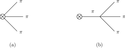
Figure 1: Diagrams contributing to the hadronic amplitude $T_{\pm\mu}$ at ${\cal O}(p^{2})$ in $\chi$PT. The crossed circle indicates the insertion of the axial–vector current.

In the limit of low $Q^{2}$ (i.e. $Q^{2}\ll M_{R}^{2}$) the resonance fields can be integrated out, and their contributions should reduce to the corrections to Eq. (23) obtained from the effective ${\cal O}(p^{4})$ interactions and higher order couplings in the standard $\chi$PT Lagrangian. In hadronic $\tau$ decays, however, we need to implement the resonance degrees of freedom explicitly because $Q^{2}\sim M_{R}^{2}$. As stated in Section 2 we assume here that the resonances $\rho$(770) and $a_{1}$(1260) give the dominant contributions to $\tau\to\pi\pi\pi\nu_{\tau}$ decays. Consequently, in addition to the usual $\chi$PT diagrams leading to Eq. (23) we include resonance–mediated contributions to the amplitude, to be evaluated through the interacting terms ${\cal L}_{2}^{\rm V/A}$ and ${\cal L}_{2}^{\rm VAP}$ of the resonance effective theory.

The relevant diagrams to be taken into account are those shown in Fig. 2. Let us start by considering the contributions given by the graphs in Figs. 2 (a) and (b), which involve only one intermediate resonance. From the interaction Lagrangian in Eq. (2), the sum of both graphs leads to

$$T_{\pm\mu}^{(1R)}=\mp\frac{\sqrt{2}\,F_{V}\,G_{V}}{3\,F^{3}}\,\left\{\,\alpha_{1}(Q^{2},s,t)\,V_{1\mu}+\alpha_{1}(Q^{2},t,s)\,V_{2\mu}+[\alpha_{2}(Q^{2},s,t)+\alpha_{2}(Q^{2},t,s)]\,Q_{\mu}\right\}\,,$$ (24)

where we have defined

$$\alpha_{1}(Q^{2},s,t) \equiv -\,3\,\frac{\displaystyle s}{\displaystyle s-M_{V}^{2}}\,+\,\left(\frac{\displaystyle 2G_{V}}{\displaystyle F_{V}}-1\right)\,\left\{\,\frac{\displaystyle 2Q^{2}-2s-u}{\displaystyle s-M_{V}^{2}}\,+\,\frac{\displaystyle u-s}{\displaystyle t-M_{V}^{2}}\,\right\}\;\;,$$

$$\alpha_{2}(Q^{2},s,t) \equiv 3\,\frac{\displaystyle G_{V}}{\displaystyle F_{V}}\,\frac{\displaystyle s}{\displaystyle Q^{2}}\,\frac{\displaystyle m_{\pi}^{2}}{\displaystyle Q^{2}-m_{\pi}^{2}}\,\frac{\displaystyle u-t}{\displaystyle s-M_{V}^{2}}\;\;.$$ (25)

As expected, the pseudoscalar form factor $\alpha_{2}(Q^{2},s,t)$ is found to vanish in the chiral limit.

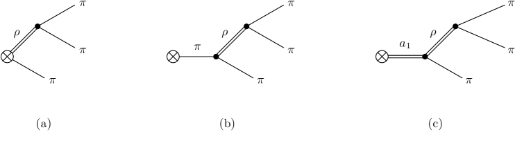
Figure 2: Resonance–mediated diagrams contributing to the hadronic amplitude $T_{\pm\mu}^{(1R)}$, (a) and (b), and $T_{\pm\mu}^{(2R)}$, (c).

The two–resonance contribution in Fig. 2 (c) can be evaluated taking into account the chiral couplings from ${\cal L}_{2}^{\rm VAP}$ in Eq. (2). We obtain :

$$T^{(2R)}_{\pm\mu}=\pm\frac{4\,F_{A}G_{V}}{3\,F^{3}}\,\frac{\displaystyle Q^{2}}{\displaystyle Q^{2}-M_{A}^{2}}\,\left[\,\beta(Q^{2},s,t)\,V_{1\mu}+\beta(Q^{2},t,s)\,V_{2\mu}\right]\;\;,$$ (26)

where

$$\beta(Q^{2},s,t)\,\equiv\,-\,3\,(\lambda^{\prime}+\lambda^{\prime\prime})\,\frac{\displaystyle s}{\displaystyle s-M_{V}^{2}}\,+\,\,F(Q^{2},s)\,\frac{\displaystyle 2Q^{2}+s-u}{\displaystyle s-M_{V}^{2}}\,+\,F(Q^{2},t)\,\frac{\displaystyle u-s}{\displaystyle t-M_{V}^{2}}\,\;\;,$$ (27)

with

$$F(Q^{2},s) = -\,\lambda_{0}\,\frac{\displaystyle m_{\pi}^{2}}{\displaystyle Q^{2}}\,+\,\lambda^{\prime}\,\frac{\displaystyle s}{\displaystyle Q^{2}}\,+\,\lambda^{\prime\prime}\;\;,$$

$$\lambda_{0} = -\,\frac{1}{\sqrt{2}}\left[4\,\lambda_{1}\,+\lambda_{2}+\frac{\lambda_{4}}{2}+\lambda_{5}\right]\;\;,$$

$$\lambda^{\prime} = \frac{1}{\sqrt{2}}\,(\lambda_{2}-\lambda_{3}+\frac{\lambda_{4}}{2}+\lambda_{5})\;\;,$$

$$\lambda^{\prime\prime} = \frac{1}{\sqrt{2}}\,(\lambda_{2}-\frac{\lambda_{4}}{2}-\lambda_{5})\;.$$ (28)

Notice that the form factor $\beta(Q^{2},s,t)$ is written in terms of only three combinations of the unknown couplings in ${\cal L}_{2}^{\rm VAP}$, namely $\lambda_{0}$, $\lambda^{\prime}$ and $\lambda^{\prime\prime}$.

The final result from our evaluation gives, accordingly, the addition of all the amplitudes considered here :

$$T_{\pm\mu}\,=\,T_{\pm\mu}^{\chi}\,+\,T_{\pm\mu}^{(1R)}\,+\,T_{\pm\mu}^{(2R)}\;\;,$$ (29)

and, for later use, if we only consider the $J^{P}=1^{+}$ mediated form factors $F_{1}$ and $F_{2}$ we will specify $T_{\pm\mu}\,|_{1^{+}}$.

3.2 Implementation of off–shell widths

The form factors in Eqs. (25) and (27) include zero–width $\rho$(770) and $a_{1}$(1260) propagator poles, leading to divergent phase–space integrals in the calculation of the $\tau\to\pi\pi\pi\nu_{\tau}$ decay width as the kinematical variables go along the full energy spectrum. The result can be regularized through the inclusion of resonance widths, which means to go beyond the leading order in the $1/N_{C}$ expansion, and implies the introduction of some additional theoretical inputs. Moreover both contributing resonances, especially the $a_{1}$(1260), are rather wide. Hence energy–dependent widths should be included in order to handle their off–shell character. This issue has been analysed in detail within the resonance chiral effective theory in Ref. [16]. For the case of spin-1 vector resonances, it is seen that one can define the off–shell width by taking into account the pole of the two–point function of the corresponding vector current that arises from the resummation of those diagrams that include an absorptive contribution of two pseudoscalars in the $s$ channel. The width is defined then as the imaginary part of this pole. In the case of the $\rho$(770) meson this procedure leads to the result

$$M_{V}\,\Gamma_{\rho}(s)\,=\,\frac{\displaystyle M_{V}^{2}\,s}{\displaystyle 96\,\pi\,F^{2}}\left[\sigma_{\pi}^{3}\,\theta(s-4\,m_{\pi}^{2})+\frac{1}{2}\,\sigma_{K}^{3}\,\theta(s-4\,m_{K}^{2})\right]\;,$$ (30)

where $\sigma_{P}=\sqrt{1-4m_{P}^{2}/s}$, and $\theta(x)$ is the step function. In the case of the $a_{1}$(1260) meson the construction following the definition above, though well defined, is much more involved. It would amount to evaluate the axial–vector–axial–vector current correlator with absorptive cuts of three pions within the resonance effective theory. This corresponds to a non–trivial two–loop calculation within a theory whose regularization is still not well defined. This calculation is far beyond our scope. In order to perform the phenomenological analysis we will introduce a chiral–based off–shell width for the $a_{1}$(1260) resonance that endows the appropriate kinematical and dynamical features :

$$M_{A}\,\Gamma_{a_{1}}(Q^{2})=M_{A}\,\Gamma_{a_{1}}(M_{A}^{2})\,\frac{\displaystyle\phi(Q^{2})}{\displaystyle\phi(M_{A}^{2})}\,\left(\frac{\displaystyle M_{A}^{2}}{\displaystyle Q^{2}}\right)^{\alpha}\,\theta(Q^{2}-9\,m_{\pi}^{2})\;,$$ (31)

where  :

$$\phi(Q^{2})\,=\,Q^{2}\int ds\,dt\;\bigg{\{}V_{1}^{2}\,|BW_{\rho}(s)|^{2}+V_{2}^{2}\,|BW_{\rho}(t)|^{2}+2\,(V_{1}\cdot V_{2})\,{\rm Re}[BW_{\rho}(s)\,BW_{\rho}(t)^{\ast}]\;\bigg{\}}\;\;,$$ (32)

and

$$BW_{\rho}(s)=\frac{M_{V}^{2}}{M_{V}^{2}-s-i\,M_{V}\,\Gamma_{\rho}(s)}$$ (33)

is the usual Breit–Wigner function for the $\rho$(770) meson resonance shape, and the energy–dependent width $\Gamma_{\rho}(s)$ is given by Eq. (30).

In conclusion, while the off-shell width of the $\rho$(770) meson does not introduce any additional free parameters on our result for $T_{\pm\mu}$, the $a_{1}$(1260) width includes two new ones, namely the on–shell width $\Gamma_{a_{1}}(M_{A}^{2})$ and the parameter $\alpha$ ruling the $Q^{2}$ behaviour in Eq. (31).

4 Asymptotic behaviour and QCD constraints

As commented at the end of Section 2, our Lagrangian ${\cal L}_{\rm R\chi T}$ in Eq. (14) does not provide an effective theory of QCD for arbitrary values of its couplings. The only tool used in its construction were relevant symmetry properties of QCD, but it is clear that the full theory should unambiguously predict the values of the coupling constants. Although it is not known how to achieve this goal from first principles, several ideas based on matching procedures have been developed [11, 17]. In this Section we show how to proceed in order to obtain information on the, a priori, unknown couplings in ${\cal L}_{2}^{\rm VAP}$.

The QCD ruled short–distance behaviour of the vector form factor in the large–$N_{C}$ limit (approximated with only one octet of vector resonances) constrains the couplings of ${\cal L}_{2}^{\rm V}$ in Eq. (2), which must satisfy [11] :

$$1\,-\,\frac{\displaystyle F_{V}\,G_{V}}{\displaystyle F^{2}} = 0\;\;.$$ (34)

In addition, the first Weinberg sum rule [18], in the limit where only the lowest narrow resonances contribute to the vector and axial–vector spectral functions, leads to

$$F_{V}^{2}-F_{A}^{2}=F^{2}\;.$$ (35)

In Ref. [11] it was also noticed that there is an additional constraint coming from the axial form factor, namely :

$$2F_{V}G_{V}\,-\,F_{V}^{2}\,=0\;,$$ (36)

that is very well satisfied by the phenomenology. However this relation is not necessarily true when we consider the inclusion of vector–pseudoscalar–axial couplings as given by ${\cal L}_{2}^{\rm VAP}$. In the following we are going to enforce the relation given in Eq. (36) and we will see what happens when we relax this last condition. From Eqs. (34,35,36), the three couplings $F_{V}$, $G_{V}$ and $F_{A}$ in Eq. (2) can be written in terms of the pion decay constant : $F_{V}=\sqrt{2}F$, $G_{V}=F/\sqrt{2}$ and $F_{A}=F$. We will adopt these results throughout this paper, unless stated otherwise.

An analogous analysis should be done in the case of the axial two–point function $\Pi_{A}^{\mu\nu}(Q^{2})$, which plays in $\tau\to\pi\pi\pi\nu_{\tau}$ processes the same role than the vector–vector current correlator does in the $\tau\rightarrow\pi\pi\nu_{\tau}$ decays, driven by the vector form factor. The goal will be to obtain QCD–ruled constraints on the new couplings of ${\cal L}_{2}^{\rm VAP}$, Eq. (11), similar to those obtained above. As these couplings do not depend on the Goldstone masses we will work in the chiral limit but our results will apply for non–zero Goldstone masses too. In the chiral limit the $\Pi_{A}^{\mu\nu}(Q^{2})$ correlator becomes transverse, hence we can write

$$\Pi_{A}^{\mu\nu}(Q^{2})=(Q^{\mu}Q^{\nu}-g^{\mu\nu}Q^{2})\,\Pi_{A}(Q^{2})\,.$$ (37)

As in the case of the pion and axial form factors, the function $\Pi_{A}(Q^{2})$ is expected to satisfy an unsubtracted dispersion relation. This implies a constraint for the $J=1$ spectral function Im$\Pi_{A}(Q^{2})$ in the asymptotic region, namely

$${\rm Im}\Pi_{A}(Q^{2})\,\,\smash{\mathop{-\!\!\!-\!\!\!-\!\!\!\longrightarrow}\limits^{\;\;\;Q^{2}\rightarrow\infty\;\;\;}}\;\;0\;\;.$$ (38)

Now, taking into account that each intermediate state carrying the appropriate quantum numbers yields a positive contribution to Im$\Pi_{A}(Q^{2})$, we have

$${\rm Im}\Pi_{A}(Q^{2})\,\geq\,-\frac{1}{3\,Q^{2}}\int d\Phi\;\left(T^{\mu}|_{1^{+}}\right)\,\left(T_{\mu}|_{1^{+}}\right)^{\ast}\,,$$ (39)

$d\Phi$ being the differential phase space for the three–pion state. The constraint in Eq. (38) then implies

$$\lim_{Q^{2}\to\infty}\;\int_{0}^{Q^{2}}ds\;\int_{0}^{Q^{2}-s}dt\;\frac{W_{A}}{(Q^{2})^{2}}=0\,,$$ (40)

where $W_{A}$ is the structure function defined in Eq. (20). It can be seen that the condition in Eq. (40) is not satisfied in general for arbitrary values of the coupling constants in the chiral interaction Lagrangian. Indeed, once $F_{V}$, $F_{A}$ and $G_{V}$ have been fixed by Eqs. (34), (35) and (36), we find that the constants $\lambda^{\prime}$ and $\lambda^{\prime\prime}$ appearing in the two–resonance contribution to the hadronic tensor are required to satisfy the relations

$$2\,\lambda^{\prime}\,-\,1 = 0\;\;,$$

$$\lambda^{\prime\prime} = 0\;\;.$$ (41)

Now we can come back to our results for $T_{\pm\mu}$ in Section 3 and enforce the QCD driven constraints on the couplings of our Effective Theory as given by Eqs. (34,35,36,41). We have :

$$\left.\left.T_{\pm\mu}^{\chi}\right|_{1^{+}}\,+\,T_{\pm\mu}^{(1R)}\right|_{1^{+}}\,=\,\mp\,\frac{2\sqrt{2}}{3F}\left[\left(\,1\,-\,\frac{\displaystyle 3}{\displaystyle 2}\,\frac{\displaystyle s}{\displaystyle s-M_{V}^{2}}\,\right)\,V_{1\mu}\,+\,\left(\,1\,-\,\frac{\displaystyle 3}{\displaystyle 2}\,\frac{\displaystyle t}{\displaystyle t-M_{V}^{2}}\,\right)\,V_{2\mu}\,\right]$$ (42)

and

$$T_{\pm\mu}^{(2R)}\,=\,\pm\,\frac{\displaystyle 2\sqrt{2}}{\displaystyle 3\,F}\,\frac{\displaystyle Q^{2}}{\displaystyle Q^{2}-M_{A}^{2}}\,\,\left[\,\beta(Q^{2},s,t)\,V_{1\mu}+\beta(Q^{2},t,s)\,V_{2\mu}\right]\;,$$ (43)

where

$$\beta(Q^{2},s,t)\, \equiv \,-\,\frac{\displaystyle 3}{\displaystyle 2}\,\frac{\displaystyle s}{\displaystyle s-M_{V}^{2}}\,+F(Q^{2},s)\,\frac{\displaystyle 2Q^{2}+s-u}{\displaystyle s-M_{V}^{2}}\,+\,F(Q^{2},t)\,\frac{\displaystyle u-s}{\displaystyle t-M_{V}^{2}}\;\;,$$

$$F(Q^{2},s)\, = \,\left(\,\frac{\displaystyle s}{\displaystyle 2Q^{2}}\,-\,\lambda_{0}\,\frac{\displaystyle m_{\pi}^{2}}{\displaystyle Q^{2}}\,\right)\;\;.$$ (44)

Thus, it turns out that the hadronic amplitude can be written in terms of only one unknown coupling parameter, namely $\lambda_{0}$.

As mentioned in Section 2, the resonance exchange approximately saturates the phenomenological values of the ${\cal O}(p^{4})$ couplings in the standard $\chi$PT Lagrangian. This allows to relate both schemes in the low energy region, and provides a check of our results in the limit $Q^{2}\ll M_{V}^{2}$. We have performed this check (see Appendix A), verifying the agreement between our expression Eq. (42) and the result obtained within $\chi$PT in Refs. [3, 19] coming from saturation by vector meson resonances of the ${\cal O}(p^{4})$ couplings :

$$\left.T_{\pm\mu}^{\chi PT}\right|_{1^{+}}\,=\,\mp\,\frac{2\sqrt{2}}{3F}\left[\left(1+\frac{3\,s}{2\,M_{V}^{2}}\right)V_{1\mu}+\left(1+\frac{3\,t}{2\,M_{V}^{2}}\right)V_{2\mu}\right]\,+\mbox{ chiral loops }\,+\,{\cal O}(p^{6})\;\;.$$ (45)

As an aside, it is worth to point out that this low–energy behaviour is not fulfilled by all phenomenological models proposed in the literature. In particular, in the widely used model by Kühn and Santamaria (KS) [4] the hadronic amplitude satisfies

$$T_{\pm\mu}^{(KS)}\;\;\smash{\mathop{-\!\!\!-\!\!\!-\!\!\!\longrightarrow}\limits^{\;\;s,t\,\ll\,M_{V}^{2}\;\;}_{\,}}\mp\,\frac{\displaystyle 2\sqrt{2}}{\displaystyle 3F}\left[\left(1+\frac{s}{M_{V}^{2}}\right)V_{1\mu}+\left(1+\frac{t}{M_{V}^{2}}\right)V_{2\mu}\right]\;.$$ (46)

Thus, while the lowest order behaviour is correct (it was constructed to be so), it is seen that the KS model fails to reproduce the $\chi$PT result at the next–to–leading order. Accordingly this model is not consistent with the chiral symmetry of QCD.

5 Phenomenology of $\tau\to\pi\pi\pi\nu_{\tau}$ processes

In this Section we discuss the ability of our Effective Theory to describe the experimental observations in $\tau\to\pi\pi\pi\nu_{\tau}$ decays, taking into account the data obtained from the measurements of $\tau\to\pi\pi\pi\nu_{\tau}$ spectra, branching ratios and structure functions.

Before proceeding let us specify which are the parameters left unknown in our evaluation of the hadronic matrix amplitude. To analyse the experimental data we will only consider the dominating $J^{P}=1^{+}$ driven axial–vector form factors, being the pseudoscalars suppressed by pion mass factors. Hence we notice that $T_{+\mu}|_{1^{+}}\,=\,-\,T_{-\mu}|_{1^{+}}$ and, accordingly, we have the same predictions for both $\tau^{-}\to\pi^{+}\pi^{-}\pi^{-}\nu_{\tau}$ and $\tau^{-}\to\pi^{-}\pi^{0}\pi^{0}\nu_{\tau}$ processes in the isospin limit. As we have shown in the previous Section, the requirement of the proper asymptotic behaviour of vector and axial–vector spectral functions consistent with QCD imposes several constraints on the coupling constants of our Lagrangian ${\cal L}_{\rm R\chi T}$ in Eq. (14) and, as a consequence, the hadronic amplitude for the decays $\tau\to\pi\pi\pi\nu_{\tau}$ only involves one adimensional unknown combination of coupling constants, $\lambda_{0}$. In addition, we have three remaining parameters, related with the $a_{1}$(1260) resonance : these are its mass $M_{A}$, its on–shell width $\Gamma_{a_{1}}(M_{A}^{2})$ and the exponent $\alpha$, which has been introduced in Eq. (31) to account for the dominating energy dependence of the off-shell $a_{1}$(1260) width. The mass of the vector octet $M_{V}$, to be identified with the $\rho$(770) mass, is better obtained from the vector form factor of the pion [14, 20] and we take here $M_{V}=775.1\,\mbox{MeV}$. In this way, we deal with four free parameters to fit the experimental data.

5.1 Fit to the ALEPH branching ratio and spectral function

In order to check the consistency of the available experimental results with the theoretical description provided by our chirally-based resonance framework we have carried out a fit of the unknown parameters entering the amplitudes. We have chosen to fit the experimental values for the $\tau^{-}\to\pi^{+}\pi^{-}\pi^{-}\nu_{\tau}$ branching ratio and normalized spectral function obtained by ALEPH [6], which quotes the unfolded spectrum for the decay including the corresponding covariance matrix. The data are collected in 57 equally spaced bins with a $3\pi$ squared invariant mass ranging from $Q^{2}=0.275$ GeV² to $Q^{2}=3.075$ GeV². We have noticed that bins $n=2$ and $n=54$ produce anomalously high $\chi^{2}$ contributions, due to their tiny errors, and we have discarded them. In addition we have fitted the total branching ratio to the value quoted by ALEPH [6], $\mbox{BR}(\tau^{-}\to\pi^{+}\pi^{-}\pi^{-}\nu_{\tau})=(9.15\pm 0.15)$%, which has been introduced as an additional fitting point. In order to control possible fake results the procedure has been carried out both with the MINUIT package [21] and with an independent minimization procedure. As output of our fit we find the four parameter set

$$\lambda_{0} = 11.9\pm 0.4\;\;,$$

$$\alpha = 2.45\pm 0.15\;\;,$$

$$M_{A} = (1.204\pm 0.007)\rm{\ GeV}\;\;,$$

$$\Gamma_{a_{1}}(M_{A}^{2}) = (0.48\pm 0.02)\rm{\ GeV}\;\;,$$ (47)

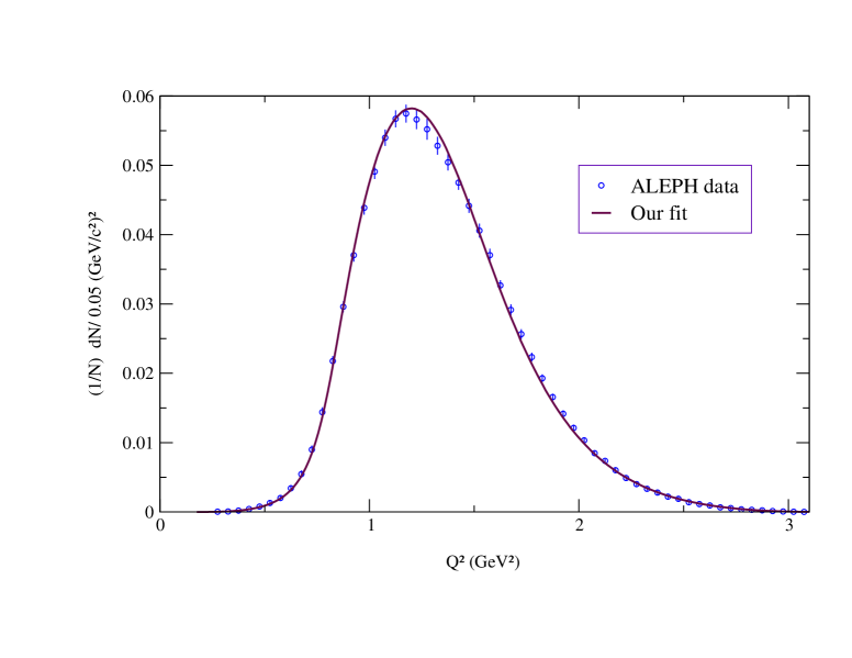
Figure 3: Fit to the ALEPH data for the normalized $\tau^{-}\to\pi^{+}\pi^{-}\pi^{-}\nu_{\tau}$ spectral function.

with $\chi^{2}/\rm{d.o.f.}=64.5/52$ (these numbers include only statistical errors). We find that the values of the parameters in Eq. (5.1) lead to $\mbox{BR}(\tau^{-}\to\pi^{+}\pi^{-}\pi^{-}\nu_{\tau})=(9.1\pm 0.3)$%. The theoretical spectrum arising from the central values of our fit, together with ALEPH data, are represented in Fig. 3. It can be seen that the agreement is good, if one considers the very small errors in the experimental data. On the other hand, the values obtained for the $a_{1}$(1260) mass and width are in good agreement with the world average values quoted by the Particle Data Group [22].

Taking into account the value of $\alpha$ in Eq. (5.1), we have carried out three additional three-parameter fits in which $\alpha$ has been fixed to the values 2, 2.5 and 3, respectively. The results are shown in Table I. Although the results clearly prefer a value of $\alpha=2.5$, one can see that the quality of the fits is reasonably similar to that of the four-parameter case, and the values of $\lambda_{0}$, $M_{A}$ and $\Gamma_{a_{1}}(M_{A}^{2})$ are not significantly modified. Thus it can be concluded that a more sophisticated evaluation of the behaviour of the off-shell $a_{1}$(1260) width should not imply a major qualitative and quantitative changes in our global analysis.

	$\alpha=2$	$\alpha=2.5$	$\alpha=3$
$\lambda_{0}$	$12.7\pm 0.4$	$11.9\pm 0.3$	$11.9\pm 0.3$
$M_{A}$	$1.242\pm 0.004$	$1.203\pm 0.003$	$1.170\pm 0.002$
$\Gamma_{a_{1}}(M_{A}^{2})$	$0.55\pm 0.02$	$0.48\pm 0.02$	$0.44\pm 0.01$
$\chi^{2}/\rm{d.o.f.}$	83.1/53	64.6/53	100.1/53
BR($\tau^{-}\to\pi^{+}\pi^{-}\pi^{-}\nu_{\tau}$)	9.11%	9.13%	9.21%

Table 1: Results of three-parameter fits to ALEPH data for fixed values of $\alpha$. $M_{A}$ and $\Gamma_{a_{1}}(M_{A}^{2})$ are given in units of GeV.

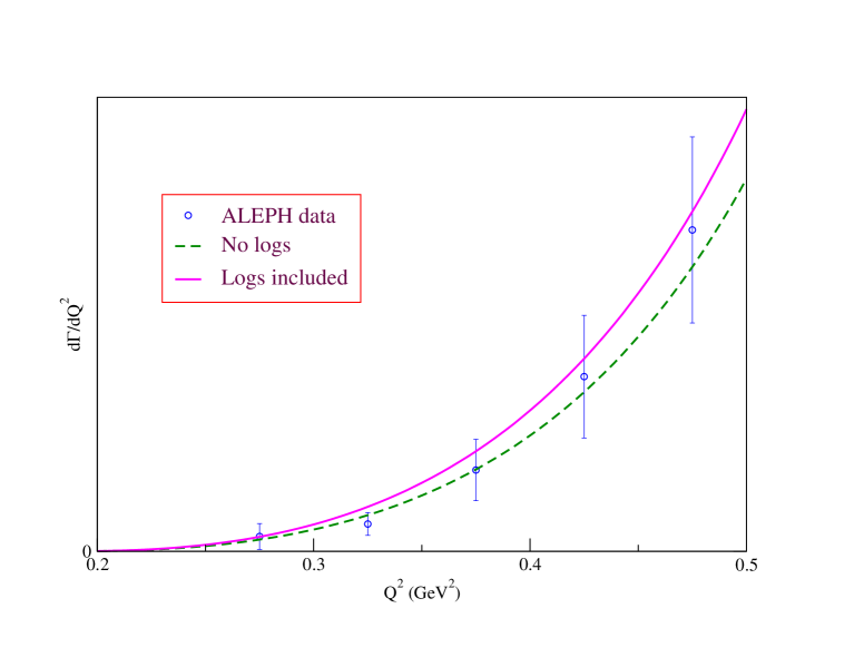
Figure 4: Theoretical curves for $\tau^{-}\to\pi^{+}\pi^{-}\pi^{-}\nu_{\tau}$ spectrum at $Q^{2}\ll M_{V}^{2}$, with and without the inclusion of chiral logs, vs. ALEPH data in the low $Q^{2}$ region [6].

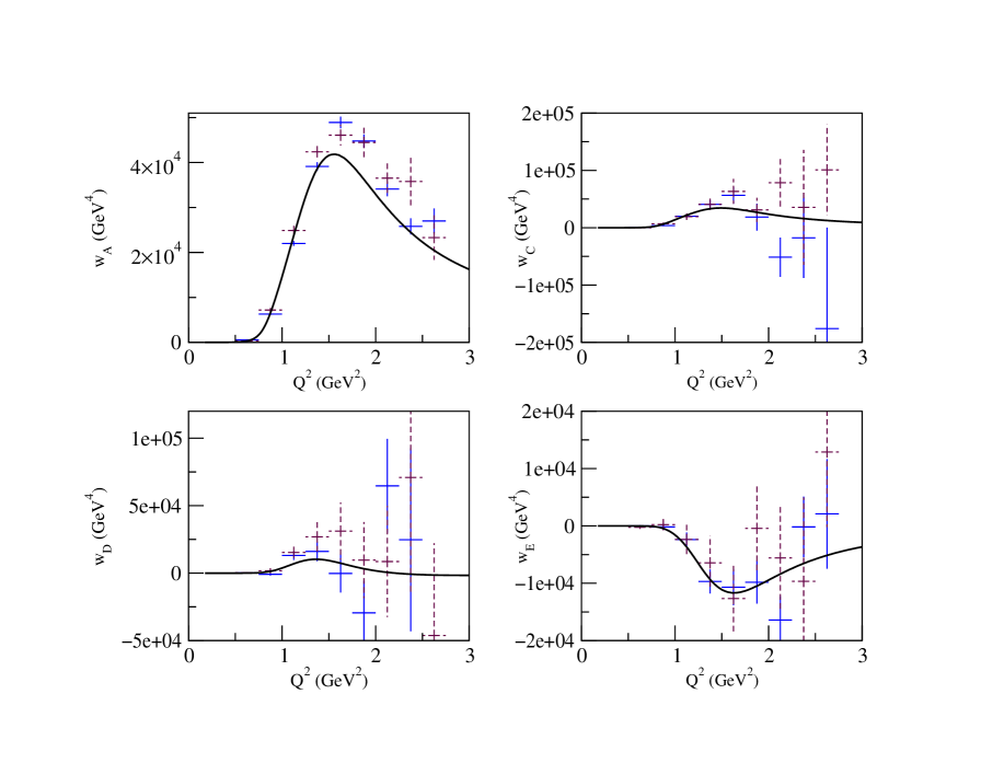
Figure 5: Theoretical values for the $w_{A}$, $w_{C}$, $w_{D}$ and $w_{E}$ integrated structure functions in comparison with the experimental data from CLEO-II (solid) and OPAL (dashed) [8]. All of them have been normalized to their respective branching ratios.

To conclude this analysis, we take a closer look to the low $Q^{2}$ region of the spectrum. In fact, in our approach we have assumed that ${\cal O}(p^{4})$ corrections arising from chiral logs are small, hence the dominant contributions to hadronic amplitudes arise from resonance exchange. Close to threshold (i.e. for $\sqrt{Q^{2}}$ well below $M_{V}$) one is able to explicitly calculate the contributions of ${\cal O}(p^{4})$ chiral logs, therefore our theoretical prediction for the spectrum in this region can be improved, and the impact of chiral logs can be numerically evaluated. In order to add these contributions to the hadronic amplitude, we have made use of the calculations performed in Ref. [3] within standard $\chi$PT. The corresponding results are sketched in Appendix A. The effect on the $\tau^{-}\to\pi^{+}\pi^{-}\pi^{-}\nu_{\tau}$ spectral function is shown in Fig. 4, where we display both the experimental values from ALEPH and the curves for the spectrum with and without the inclusion of ${\cal O}(p^{4})$ chiral logs. It can be seen that the corrections produce a slight enhancement of the spectral function. However, given the size of the experimental errors, the quality of the agreement with ALEPH data is unchanged.

When enforcing the asymptotic conditions of QCD in Section 4, we pointed out that the relation in Eq. (36) is not necessarily true when the vertices in ${\cal L}_{2}^{\rm VAP}$ are considered, because the latter contribute to the axial form factor. If we do not take into account that constraint we can perform a 5 parameter fit to the ALEPH data that gives :

$$\lambda_{0} = 11.0\pm 1.7\;\;,$$

$$\alpha = 2.55\pm 0.15\;\;,$$

$$M_{A} = (1.19\pm 0.02)\rm{\ GeV}\;\;,$$

$$\Gamma_{a_{1}}(M_{A}^{2}) = (0.47\pm 0.02)\rm{\ GeV}\;\;,$$

$$\frac{\displaystyle G_{V}}{\displaystyle F_{V}} = 0.49\pm 0.03\;\;\;,$$ (48)

and $\chi^{2}/\rm{d.o.f.}=63.7/51$. We see that the ratio $G_{V}/F_{V}$ is consistent with the value given by Eq. (36) within the error. Hence we confirm that the experimental data favour the $F_{V}=2G_{V}$ constraint.

Finally a word of caution has to be said about the value of $\lambda_{0}$. The only dependence of the amplitude on this parameter is given by the function $F(Q^{2},s)$ in Eq. (3.1) where, as can be seen, $\lambda_{0}$ is multiplied by the squared mass of the pion. Hence the sensibility of the observables in $\tau\to\pi\pi\pi\nu_{\tau}$ on $\lambda_{0}$ is very much covered up. Tau decays into kaons would provide a better testing field to find out on $\lambda_{0}$ and check the results against the values from our fits. We consider that our result on this parameter has to be taken with care.

5.2 Description of structure functions

Structure functions provide a full description of the hadronic tensor $T_{\mu}T_{\nu}^{*}$ in the hadron rest frame. There are 16 real valued structure functions in $\tau\rightarrow P_{1}P_{2}P_{3}\,\nu_{\tau}$ decays ($P_{i}$ is short for a pseudoscalar meson), most of which can be determined by studying angular correlations of the hadronic system. Four of them carry information on the $J^{P}=1^{+}$ transitions only : $w_{A}$, $w_{C}$, $w_{D}$ and $w_{E}$ (we refer the reader to Ref. [15] for their precise definitions). Indeed, for the $\tau\to\pi\pi\pi\nu_{\tau}$ processes, other structure functions either vanish identically, or involve the pseudoscalar form factor $F_{P}$, which appears to be strongly suppressed above the very low–energy region due to its proportionality to the squared pion mass.

Both CLEO-II and OPAL have measured the four structure functions quoted above for the $\tau^{-}\to\pi^{-}\pi^{0}\pi^{0}\nu_{\tau}$ process, while concluding that other functions are consistent with zero within errors. Hence we can proceed to compare those experimental results with the description that provides our theoretical approach. In our expressions for the structure functions we input the values of the parameters obtained from the fit in Eq. (5.1), getting the theoretical curves shown in Fig. 5. The latter are compared with the experimental data quoted by CLEO and OPAL [8]. For $w_{C}$, $w_{D}$ and $w_{E}$, it can be seen that we get a good agreement in the low $Q^{2}$ region, while for increasing energy the experimental errors become too large to state any conclusion (moreover, there seems to be a slight disagreement between both experiments at some points).

On the other hand, in the case of the integrated structure function $w_{A}$, the quoted experimental errors are smaller, and the theoretical curve seems to lie somewhat below the data for $Q^{2}\stackrel{{\scriptstyle>}}{{{}_{\sim}}}1.5\,\mbox{GeV}^{2}$. However, it happens that $w_{A}$ contains essentially the same information about the hadronic amplitude as the spectral function $d\Gamma/dQ^{2}$. This becomes clear by looking at Eq. (19) if the scalar structure function $W_{SA}$ is put to zero (remember that it should be suppressed by a factor ${\cal O}(m_{\pi}^{2}/Q^{2})$). Taking into account that $w_{A}$ is given by

$$w_{A}(Q^{2})=\int ds\,dt\;W_{A}(Q^{2},s,t)\,\,\;,$$ (49)

where $W_{A}$ is the structure function previously introduced in Eq. (20), one simply has

$$\frac{\displaystyle d\Gamma}{\displaystyle dQ^{2}}\,=\,\frac{G_{F}^{2}\,|V_{ud}|^{2}}{384\,(2\pi)^{5}\,M_{\tau}}\;\left(\,\frac{\displaystyle M_{\tau}^{2}}{\displaystyle Q^{2}}-1\,\right)^{2}\left(1\,+\,2\,\frac{Q^{2}}{M_{\tau}^{2}}\right)\;\;w_{A}(Q^{2})\;\;.$$ (50)

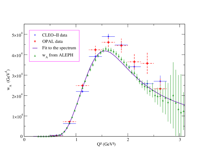
Figure 6: Comparison between the experimental data for $w_{A}$, from $\tau^{-}\to\pi^{-}\pi^{0}\pi^{0}\nu_{\tau}$, quoted by CLEO-II and OPAL [8] and the values arising from ALEPH measurements of $\tau^{-}\to\pi^{+}\pi^{-}\pi^{-}\nu_{\tau}$ spectral functions [6]. The solid line is obtained from our four-parameter fit of the spectrum (see text).

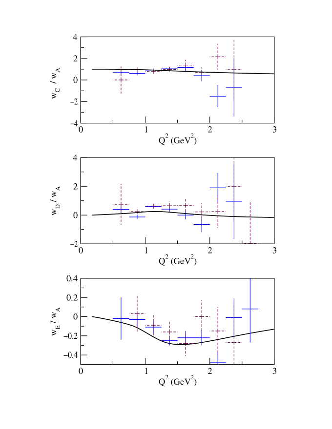
Figure 7: Experimental data for $w_{C}$, $w_{D}$ and $w_{E}$ integrated structure functions, normalized to $w_{A}$. Solid (dashed) bars correspond to the values quoted by CLEO-II (OPAL) [8].

In this way one can compare the measurements of $w_{A}$ quoted by CLEO-II and OPAL with the data obtained by ALEPH for the spectral function, conveniently translated into $w_{A}$. This is represented in Fig. 6, where it can be seen that some of the data from the different experiments do not agree with each other within errors. Notice that, due to phase space suppression, the factor of proportionality between $w_{A}(Q^{2})$ and $d\Gamma/dQ^{2}$ in Eq. (50) goes to zero for $Q^{2}\rightarrow M_{\tau}^{2}$, therefore the error bars in the ALEPH points become enhanced toward the end of the spectrum. Notwithstanding, up to $Q^{2}\simeq 2.5$ GeV², it is seen that ALEPH errors are still smaller than those corresponding to the values quoted by CLEO-II and OPAL. On this basis, we have chosen here to take the data obtained by ALEPH to fit the unknown theoretical parameters in the hadronic amplitude. Finally, notice that a non vanishing contribution of $W_{SA}$ (which is a positive quantity) cannot help to solve the experimental discrepancies, as it would go in the wrong direction.

In the analysis of data carried out by the CLEO Collaboration [23] onto their $\tau^{-}\to\pi^{-}\pi^{0}\pi^{0}\nu_{\tau}$ results it was concluded that the data was showing large contributions from intermediate states involving the isoscalar mesons $f_{0}$(600), $f_{0}$(1370) and $f_{2}$(1270). Their analysis was done in a modelization of the axial–vector form factors that included Breit–Wigner functions in a Kühn and Santamaria inspired model. Our results in the Effective Theory framework show that, within the present experimental errors, there is no evidence of relevant contributions in $\tau\to\pi\pi\pi\nu_{\tau}$ decays beyond those of the $\rho$(770) and $a_{1}$(1260) resonances.

We also find interesting to study the integrated structure functions $w_{C}$, $w_{D}$ and $w_{E}$, normalized to $w_{A}$. This quantities should be less sensitive to the parameterization of the $a_{1}$(1260) width, and do not depend on the global normalization used by each experiment (which could be the origin of the partial discrepancies in the values for $w_{A}$). The corresponding comparison between the theoretical and experimental results are plotted in Fig. 7, where once again it is seen that our predictions are in good agreement with the experimental data within their present errors.

6 Conclusions

The hadronization of QCD currents yields relevant information on non–perturbative features of low–energy Quantum Chromodynamics. At $E\ll M_{V}$, $\chi$PT has provided model–independent knowledge on the corresponding form factors, but when resonance degrees of freedom become active, at $E\sim M_{V}$, they have to be properly included into the Effective Theory and $\chi$PT is no longer the appropriate scheme to work with. While thorough parameterizations of the hadron matrix amplitudes involving resonances have been used in the past, most of them implement Breit–Wigner functions in order to provide the dynamical description of the resonances and, as far as we know, there is no deductive connexion between those functions and QCD. Hadronic $\tau$ decays take place in the bulk of the energy resonance region and, moreover, several experiments in the last years have payed attention to them, supplying a good quality and quantity of data. Therefore they constitute an interesting subject of research to which we have turned over.

In this article we have proposed an Effective Theory approach in order to evaluate the dominant form factors in $\tau\to\pi\pi\pi\nu_{\tau}$ decays, and our results have been compared with the experimental figures. To proceed to the construction of the relevant Effective Theory we have relied in the R$\chi$T proposed in Ref. [10], which has been improved here by implementing the necessary vector–axial–vector–Goldstone interactions ${\cal L}_{2}^{\rm VAP}$ in Eqs. (11, 2). The basic principles underlying this procedure are the all–important chiral symmetry of massless QCD, that drives the interaction of Goldstone bosons at low–energy, and the unitary flavour symmetry of the octets of resonances. Once specified our interaction Lagrangian we have proceeded to evaluate the axial–vector current form factors in $\tau\to\pi\pi\pi\nu_{\tau}$ processes. It is clear though that, up to this point, the Lagrangian ${\cal L}_{\rm R\chi T}$ is not a proper Effective Theory of QCD for arbitrary values of the coupling constants. Hence we have implemented the consequences of the asymptotic behaviour of vector and axial–vector spectral functions of the underlying QCD into the corresponding form factors. This procedure has fixed up several constraints onto the couplings, yielding an Effective Theory more germane to QCD.

After applying this method we are left with four unknown parameters in our results for the axial–vector form factors. We have used the ALEPH data on $\tau^{-}\to\pi^{+}\pi^{-}\pi^{-}\nu_{\tau}$ to perform a fit to its branching ratio and spectral function, rendering values for the mass and on–shell width of the $a_{1}$(1260) resonance. Once the parameters in the theoretical expressions of the form factors have been determined, we have evaluated the integrated structure functions $w_{A}$, $w_{C}$, $w_{D}$ and $w_{E}$ measured by the CLEO-II and OPAL experiments [8]. We have found a good description of data, though there appear to be some inconsistencies between the results provided by the different experiments.

In summary we have provided an Effective Theory based evaluation of the axial–vector form factors in $\tau\to\pi\pi\pi\nu_{\tau}$ decays that gives an appropriate account of the main features of the experimental data. The procedure does not rely in any modelization of the form factors, as it has been done in the past, but in a field theory construction that embodies the relevant features of QCD in the resonance energy region, showing that this is a compelling framework to work with.

Appendix A The ${\cal O}(p^{4})$ $\chi$PT result for $\tau^{-}\to\pi^{+}\pi^{-}\pi^{-}\nu_{\tau}$

In the very low $Q^{2}$ region (typically $E\ll M_{V}$), our results for the hadronic amplitudes in $\tau\to\pi\pi\pi\nu_{\tau}$ can be compared with those obtained in standard $\chi$PT. Here we will rely on the analysis in Ref. [3], where these calculations have been performed in detail up to ${\cal O}(p^{4})$.

The ${\cal O}(p^{4})$ hadronic matrix element $T_{\mu}$ involves renormalized coupling constants $\ell_{i}^{r}(\mu)$, which have to be determined experimentally at a given renormalization scale. It is seen that these couplings can be related to finite and scale-independent quantities $\bar{\ell}_{i}$ [2] according to :

$$\bar{\ell}_{i}=\left(\frac{\gamma_{i}}{32\pi^{2}}\right)^{-1}\ell_{i}^{r}(\mu)-\ln\frac{m_{\pi}^{2}}{\mu^{2}}\;,$$ (A.1)

where the coefficients $\gamma_{i}$ arise from the corresponding renormalization group equations. In the resonance chiral effective theory, the constants $\bar{\ell}_{i}$ are assumed to be saturated by resonance exchange, which at low energies induces the local $\chi$PT Lagrangian of ${\cal O}(p^{4})$ for the light pseudoscalar mesons [10]. In this way, after considering the relations (34), imposed by QCD, one gets

$$\bar{\ell}_{1} = -48\pi^{2}\frac{F^{2}}{M_{V}^{2}}-\ln\frac{m_{\pi}^{2}}{M_{V}^{2}}\;\;,$$

$$\bar{\ell}_{2} = 24\pi^{2}\frac{F^{2}}{M_{V}^{2}}-\ln\frac{m_{\pi}^{2}}{M_{V}^{2}}\;\;,$$

$$\bar{\ell}_{4} = -\ln\frac{m_{\pi}^{2}}{M_{V}^{2}}\;\;,$$

$$\bar{\ell}_{6} = 96\pi^{2}\frac{F^{2}}{M_{V}^{2}}-\ln\frac{m_{\pi}^{2}}{M_{V}^{2}}\;\;.$$ (A.2)

Now, from the expressions quoted in Ref. [3], the $J^{P}=1^{+}$ piece of the hadronic amplitude for the decay $\tau^{-}\to\pi^{+}\pi^{-}\pi^{-}\nu_{\tau}$ is found to be

$$\left.T_{+\mu}^{\chi PT}\right|_{1^{+}}\, = \,-\,\frac{2\sqrt{2}}{3F}\,V_{1\mu}\,\Bigg{\{}1+\frac{3s}{2M_{V}^{2}}+\frac{1}{32\pi^{2}F^{2}}\bigg{[}-\frac{2}{3}\,s+\,3\,t-u-3\,m_{\pi}^{2}-(s+m_{\pi}^{2})\,F(s/m_{\pi}^{2})$$ (A.3)

$$\;\;\;\;\;\;\;\;\;\;\;\;\;\;\;\;\;\;\;\;\;\;\;\;\;\;\;\;\;\;\;\;\;\;\;\;\;\;\;\;\;\;\;\;\;\;\;\;\;\;+(3\,t-2\,m_{\pi}^{2})\,F(t/m_{\pi}^{2})-(u-2\,m_{\pi}^{2})\,F(u/m_{\pi}^{2})$$

$$\;\;\;\;\;\;\;\;\;\;\;\;\;\;\;\;\;\;\;\;\;\;\;\;\;\;\;\;\;\;\;\;\;\;\;\;\;\;\;\;\;\;\;\;\;\;\;\;\;\;+(s-3t+u-m_{\pi}^{2})\,\ln\frac{m_{\pi}^{2}}{M_{V}^{2}}\,\bigg{]}\Bigg{\}}$$

$$\,-\,\frac{2\sqrt{2}}{3F}\,V_{2\mu}\,\Bigg{\{}\;\;s\longleftrightarrow t\;\;\Bigg{\}}+{\cal O}(p^{6})\;\;,$$

where

$$F(x)=\sigma\,\ln\frac{1-\sigma}{1+\sigma}\;\;,\hskip 28.45274pt\sigma(x)=\sqrt{1-4/x}\;\;,$$ (A.4)

and the kinematical invariants $s$ and $t$ are defined as in Section 3. The first two terms in the curly brackets are those explicitly quoted in Eq. (45).

References

-
[1]
S. Weinberg, PhysicaA 96 (1979) 327;
J. Gasser and H. Leutwyler, Annals Phys. 158 (1984) 142. - [2] J. Gasser and H. Leutwyler, Nucl. Phys. B 250 (1985) 465.
- [3] G. Colangelo, M. Finkemeier and R. Urech, Phys. Rev. D 54 (1996) 4403 [arXiv:hep-ph/9604279].
- [4] J. H. Kühn and A. Santamaria, Z. Phys. C 48 (1990) 445.
-
[5]
R. Fischer, J. Wess and F. Wagner,
Z. Phys. C 3 (1980) 313;
A. Pich, Phys. Lett. B 196 (1987) 561;
A. Pich, “QCD Tests From Tau Decay Data”, SLAC Rep.-343 (1989) 416;
N. Isgur, C. Morningstar and C. Reader, Phys. Rev. D 39 (1989) 1357;
J. J. Gomez- Cadenas, M. C. Gonzalez-Garcia and A. Pich, Phys. Rev. D 42 (1990) 3093;
M. Feindt, Z. Phys. C 48 (1990) 681;
R. Decker, E. Mirkes, R. Sauer and Z. Was, Z. Phys. C 58 (1993) 445;
L. Beldjoudi and T. N. Truong, Phys. Lett. B 344 (1995) 419 [arXiv:hep-ph/9411424]. - [6] R. Barate et al. [ALEPH Collaboration], Eur. Phys. J. C 4 (1998) 409.
- [7] P. Abreu et al. [DELPHI Collaboration], Phys. Lett. B 426 (1998) 411.
-
[8]
K. Ackerstaff et al. [OPAL Collaboration],
Z. Phys. C 75 (1997) 593;
T. E. Browder et al. [CLEO Collaboration], Phys. Rev. D 61 (2000) 052004 [arXiv:hep-ex/9908030]. -
[9]
S. R. Coleman, J. Wess and B. Zumino,
Phys. Rev. 177 (1969) 2239;
C. G. Callan, S. R. Coleman, J. Wess and B. Zumino, Phys. Rev. 177 (1969) 2247. - [10] G. Ecker, J. Gasser, A. Pich and E. de Rafael, Nucl. Phys. B 321 (1989) 311.
- [11] G. Ecker, J. Gasser, H. Leutwyler, A. Pich and E. de Rafael, Phys. Lett. B 223 (1989) 425.
- [12] G. ’t Hooft, Nucl. Phys. B 72 (1974) 461.
- [13] E. Witten, Nucl. Phys. B 160 (1979) 57.
- [14] F. Guerrero and A. Pich, Phys. Lett. B 412 (1997) 382 [arXiv:hep-ph/9707347]; J. J. Sanz-Cillero and A. Pich, Eur. Phys. J. C 27 (2003) 587 [arXiv:hep-ph/0208199].
- [15] J. H. Kühn and E. Mirkes, Z. Phys. C 56 (1992) 661 [Erratum-ibid. C 67 (1995) 364].
- [16] D. Gómez Dumm, A. Pich and J. Portolés, Phys. Rev. D 62 (2000) 054014 [arXiv:hep-ph/0003320].
-
[17]
M. Knecht and A. Nyffeler, Eur. Phys. J. C 21
(2001) 659 [arXiv:hep-ph/0106034];
A. Pich, “Colorless mesons in a polychromatic world”, Proc. The Phenomenology of Large N(c) QCD, Ed. R. Lebed, p. 239, World Scientific, Singapore (2002) [arXiv:hep-ph/0205030];
G. Amorós, S. Noguera and J. Portolés, Eur. Phys. J. C 27 (2003) 243 [arXiv:hep-ph/0109169];
P. D. Ruiz-Femenia, A. Pich and J. Portolés, JHEP 0307 (2003) 003 [arXiv:hep-ph/0306157]. - [18] S. Weinberg, Phys. Rev. Lett. 18 (1967) 507.
- [19] R. Decker, M. Finkemeier and E. Mirkes, Phys. Rev. D 50 (1994) 6863 [arXiv:hep-ph/9310270].
-
[20]
A. Pich and J. Portolés, Phys. Rev. D 63 (2001) 093005
[arXiv:hep-ph/0101194];
A. Pich and J. Portolés, Nucl. Phys. Proc. Suppl. 121 (2003) 179 [arXiv:hep-ph/0209224]. - [21] F. James and M. Roos, Comput. Phys. Commun. 10 (1975) 343.
- [22] K. Hagiwara et al. [Particle Data Group Collaboration], Phys. Rev. D 66 (2002) 010001.
- [23] D. M. Asner et al. [CLEO Collaboration], Phys. Rev. D 61 (2000) 012002 [arXiv:hep-ex/9902022].