OSU-HEP-03-14

December 2003

TeV–Scale Horizontal Symmetry and the
Slepton Mass Problem of Anomaly Mediation

O.C. Anoka,^a, K.S. Babu^a, and I. Gogoladze^a,b,

^a Department of Physics, Oklahoma State University
Stillwater, OK 74078, USA

^b Department of Physics, University of Notre Dame
Notre Dame, IN 46556, USA

We propose a new scenario for solving the tachyonic slepton mass problem of anomaly mediated supersymmetry breaking models with a non–Abelian horizontal gauge symmetry broken at the TeV scale. A specific model based on $SU(3)_{H}$ horizontal symmetry is presented wherein the sleptons receive positive mass–squared from the asymptotically free $SU(3)_{H}$ gauge sector. Approximate global symmetries present in the model strongly suppress flavor changing processes induced by the horizontal vector gauge bosons. The model predicts $m_{h}\lesssim 120$ GeV for the lightest Higgs boson mass, $\tan{\beta}\simeq 4$, and $M_{V}=1-4$ TeV for the $SU(3)_{H}$ gauge boson masses. The lightest SUSY particle is found to be the neutral Wino, which is a candidate for cold dark matter.

1 Introduction

Supersymmetry provides an elegant solution to the gauge hierarchy problem of the standard model. To be realistic, it must however be a broken symmetry. There are several ways of achieving supersymmetry (SUSY) breaking. Anomaly mediated SUSY breaking (AMSB) is an attractive and predictive scenario which has the virtue that it can solve the SUSY flavor problem [1, 2]. This scenario assumes that SUSY breaking takes place in a hidden or $sequestered$ sector. The MSSM superfields are confined to a 3–brane in a higher dimensional bulk space–time separated from the sequestered sector by extra dimensions. A rescaling super–Weyl anomaly generates coupling of the auxiliary field of the gravity multiplet to the gauginos and the scalars of the MSSM, with the couplings determined by the SUSY renormalization group equations (RGE). Since the rescaling anomaly is UV insensitive, the pattern of SUSY breaking masses at any energy scale is governed only by the physics at that scale [1–3]. Arbitrary flavor structure in the SUSY scalar spectrum at high energies gets washed out at low energies. This ultraviolet insensitivity provides an elegant solution to the SUSY flavor problem.

In anomaly mediated supersymmetry breaking models, the masses of the scalar components of the chiral supermultiplets are given by [1, 2]

$$(m^{2})^{\phi_{j}}_{\phi_{i}}=\frac{1}{2}M_{aux}^{2}\left[\beta(Y)\frac{\partial}{\partial{Y}}\gamma^{\phi_{j}}_{\phi_{i}}+\beta(g)\frac{\partial}{\partial{g}}\gamma^{\phi_{j}}_{\phi_{i}}\right].$$ (1)

In the above equation summations over the gauge couplings $g$ and the Yukawa couplings $Y$ are assumed. $\gamma^{\phi_{j}}_{\phi_{i}}$ are the one–loop anomalous dimensions, $\beta(Y)$ is the beta function for the Yukawa coupling $Y$, and $\beta(g)$ is the beta function for the gauge coupling $g$. $M_{aux}$ is the vacuum expectation value of a “compensator superfield” [1] which sets the scale of SUSY breaking. The gaugino mass $M_{g}$ associated with the gauge group with coupling $g$ is given by [1, 2]

$$M_{g}=\frac{\beta{(g)}}{g}M_{aux}.$$ (2)

The trilinear soft supersymmetry breaking term $A_{Y}$ corresponding to the Yukawa coupling $Y$ is given by [1, 2]

$$A_{Y}=-\frac{\beta{(Y)}}{Y}M_{aux}.$$ (3)

In the simplest scenario for generating the $\mu$ term, which we adopt in this paper, the contribution to the Higgs mixing parameter (the $B$-term) is given by [1]

$$B = -\left(\gamma_{H_{u}}+\gamma_{H_{d}}\right)M_{aux}.$$ (4)

The one–loop anomalous dimensions $\gamma_{H_{u}}$ and $\gamma_{H_{d}}$ of the $H_{u}$ and $H_{d}$ fields are given in the Appendix (see Eqs. (45), (46)). Similar relations hold for other bilinear terms in the SUSY breaking Lagrangian.

An attractive feature of the AMSB scenario is that it can naturally solve the cosmological gravitino abundance problem which tends to destroy the success of big bang cosmology in generic supergravity models [4]. From Eqs. (1) and (2) it follows that the masses of the squarks, sleptons and the gauginos are all of order $\frac{M_{aux}}{16\pi^{2}}$. The gravitino mass, on the other hand, is $M_{gravitino}\sim M_{aux}$, which is naturally in the range 10 TeV – 100 TeV in AMSB models (for MSSM sparticle masses of order 100 GeV – 1 TeV). This is in contrast with $M_{gravitino}\sim M_{SUSY}\sim$ TeV in generic supergravity models. With a mass in the range 10 TeV – 100 TeV, the gravitino lifetime is less than a second, which suggests that the success of the big bang nucleosynthesis will be preserved in AMSB scenario [5]. Furthermore, the decay of the moduli fields present in the model (as well as the gravitino) will produce neutralinos, especially the neutral Winos, with the right abundance to make it a viable cold dark matter candidate [6].

In the minimal scenario, it turns out that AMSB induces negative mass–squared for the sleptons. Such a scenario is excluded since it would break electromagnetism. The reason for the negative mass–squared can be understood as follows. There are two sources for slepton masses in AMSB, the Yukawa part and the gauge part (Cf: Eq.. (1)). For the first two families the Yukawa couplings are negligible and the dominant contributions arise proportional to the gauge beta function. Since in the minimal supersymmetric standard Model (MSSM) the $SU(2)_{L}$ and the $U(1)_{Y}$ gauge couplings are not asymptotically free, their gauge beta functions are positive. This makes the slepton mass–squared negative. In the squark sector, the masses are positive because $SU(3)_{C}$ gauge theory is asymptotically free.

Several possible ways of avoiding the slepton mass problem of AMSB have been suggested. A non–decoupling universal bulk contribution to all the scalar masses is a widely studied option [1–3, 5–8]. While this will make the minimal model phenomenologically consistent, the UV insensitivity of AMSB is no longer guaranteed. It is therefore interesting to investigate variations of the minimal model which maintain the UV insensitivity but provide positive mass–squared for the sleptons from physics at the TeV scale. This is what we pursue in this paper.

One way to avoid the negative slepton mass problem with TeV scale physics is to increase the Yukawa contributions in Eq. (1). This can be achieved by introducing new particles at the TeV scale with large Yukawa couplings to the lepton fields. This possibility was studied in Ref. [9] where the MSSM spectrum was extended to include 3 pairs of Higgs doublets, four singlets and a vector–like pair of color–triplets near the weak scale. The Yukawa contributions can also be enhanced by invoking $R$–parity violating couplings in the MSSM [10]. Unfortunately such a theory would generate unacceptably large neutrino masses. Yet another possibility is to make use of the positive $D$–term contributions from a $U(1)$ gauge symmetry broken at the weak scale. This was achieved by adding TeV scale Fayet–Iliopoulos terms explicitly to the theory in Ref. [11]. New $D$–term contributions generated in a controlled fashion by the breaking of $U(1)_{B-L}$ at an arbitrary high scale may also provide positive contributions to the slepton masses [12, 13]. A low scale ancillary $U(1)$ as a solution to the problem has been studied in Ref. [14]. Effective supersymmetric theories which are devoid of the negative slepton mass problem of AMSB with new dynamics at the 10 TeV scale have been studied in Ref. [15]. Non–decoupling effects of heavy fields at higher orders have been analyzed in AMSB models in Ref. [16] as an attempt to solve the slepton mass problem.

The purpose of this paper is to suggest and investigate the possibility of solving the negative slepton mass problem by making the gauge contribution in Eq. (1) positive. This can only be achieved by introducing a new non–Abelian gauge symmetry for leptons with negative gauge beta function. We point out that an $SU(3)_{H}$ horizontal symmetry acting on the lepton multiplets has all the desired properties for achieving this. We show that such an $SU(3)_{H}$ horizontal symmetry broken at the TeV scale is consistent with rare leptonic processes owing to the emergence of approximate global symmetries.

The specific AMSB model we study is quite predictive. The lightest Higgs boson mass is predicted to be $m_{h}\lesssim 120$ GeV, and the parameter $\tan{\beta}$ is found to be $\tan{\beta}\simeq 4$. The model predicts the existence of new particles associated with the $SU(3)_{H}$ symmetry breaking sector. The $SU(3)_{H}$ vector bosons have masses of order 1–4 TeV. These particles should be accessible experimentally at the LHC.

The plan of the paper is as follows. In Section 2 we introduce our model. In section 3 we analyze the Higgs potential of the model. Here we derive the limits on $\tan{\beta}$ and $m_{h}$. In section 4 we present the SUSY spectrum of the model and show how the sleptons acquire positive masses. Numerical results for the full spectrum of the model are given in Section 5. In Section 6 we outline the most significant experimental consequences of the model. In Section 7 we comment on the possible origins of the $\mu$ and the $B\mu$ terms. Section 8 has our conclusions. In an Appendix we give the relevant beta functions, anomalous dimensions as well as the soft masses.

2 $SU(3)_{H}$ Horizontal Symmetry

In this section we present our model. Since our aim is to have positive contributions to the slepton masses from the gauge sector, we are naturally led to a leptonic horizontal symmetry that is asymptotically free. Our model is based on the gauge group $SU(3)_{C}\otimes SU(2)_{L}\otimes U(1)_{Y}\otimes SU(3)_{H}$, where $SU(3)_{H}$ is a horizontal symmetry acting on the leptons. The left–handed lepton doublets and the antilepton singlets transform as fundamental representations of the $SU(3)_{H}$ gauge symmetry. The theory is made anomaly free by introducing three Higgs multiplets ($\Phi_{1}$, $\Phi_{2}$, $\Phi_{3}$) which transform as antifundamental representations of $SU(3)_{H}$ and as singlets of the standard model. These fields are sufficient for breaking the $SU(3)_{H}$ symmetry completely near the TeV scale. The particle content of the model and the transformation properties under the gauge group $SU(3)_{C}\otimes SU(2)_{L}\otimes U(1)_{Y}\otimes SU(3)_{H}$ are presented in Table 1. It turns out that the Higgs potential involving these $\Phi_{i}$ fields exhibits a global $SU(3)_{G}$ symmetry. We take advantage of this global symmetry to suppress potentially large flavor changing neutral current processes mediated by the $SU(3)_{H}$ gauge bosons. The last column in Table 1 lists the transformation properties under the global $SU(3)_{G}$ symmetry (The Yukawa couplings of the model reduce the global $SU(3)_{G}$ down to $U(1)$.) The fields $\eta_{i}$ and $\bar{\eta}_{i}$ are introduced to facilitate $SU(3)_{H}$ symmetry breaking within our AMSB framework.

Superfield	$SU(3)_{C}$	$SU(2)_{L}$	$U(1)_{Y}$	$SU(3)_{H}$	$SU(3)_{G}$
$Q_{i}$	$3$	$2$	$\,\,\,\,\frac{1}{6}$	$1$	$1$
$u^{c}_{i}$	$\bar{3}$	$1$	$-\frac{2}{3}$	$1$	$1$
$d^{c}_{i}$	$\bar{3}$	1	$\,\,\,\,\frac{1}{3}$	$1$	$1$
$L_{\alpha}$	$1$	$2$	$-\frac{1}{2}$	$3$	$1$
$e^{c}_{\alpha}$	$1$	$1$	$1$	$3$	$1$
$H_{u}$	$1$	$2$	$\,\,\,\,\frac{1}{2}$	$1$	$1$
$H_{d}$	1	$2$	$-\frac{1}{2}$	$1$	$1$
$\Phi^{\alpha}_{i}$	$1$	$1$	$0$	$\bar{3}$	$3$
$\eta_{i}$	$1$	$1$	$0$	$\bar{3}$	$3$
$\bar{\eta}_{i}$	$1$	$1$	$0$	$3$	$\bar{3}$

Table 1: Particle content and charge assignment of the model. $SU(3)_{G}$ in the last column is a softly broken global symmetry present in the model. The indices $i$ and $\alpha$ take values $i,\alpha$ = $1-3$.

Note that the quarks are neutral under $SU(3)_{H}$. This is necessitated by the requirements that $SU(3)_{H}$ be asymptotically free. A separate $SU(3)_{H^{\prime}}$ acting on the quarks is a possible quark–lepton symmetric extension of the model. But we do not pursue such an extension here.

The superpotential of the model consistent with the gauge symmetries and the global $SU(3)_{G}$ symmetry is given by:

$$W = \left(Y_{u}\right)_{ij}Q_{i}H_{u}u_{j}^{c}+\left(Y_{d}\right)_{ij}Q_{i}H_{d}d_{j}^{c}+\mu H_{u}H_{d}$$ (5)

$$+ \kappa\Phi^{\alpha}_{1}\Phi^{\beta}_{2}\Phi^{\gamma}_{3}\epsilon_{\alpha\beta\gamma}+\lambda\eta_{a}^{\alpha}\eta_{b}^{\beta}\Phi_{c}^{\gamma}\epsilon_{\alpha\beta\gamma}\epsilon^{abc}+M_{\eta}\eta_{a}{\bar{\eta}}_{a}.$$

Here $\alpha$, $\beta$, $\gamma$ =1, 2, 3 are $SU(3)_{H}$ indices, $i,j$ = 1, 2, 3 are family indices, and $a,b,c$ = 1, 2, 3 are $SU(3)_{G}$ indices. The mass parameters $\mu$ and $M_{\eta}$ are of order TeV, which has a natural origin in AMSB [1]. We will comment on possible origin of these terms in Sec. 7.

In the $SU(3)_{H}$ symmetric limit the leptons are all massless. They obtain their masses from the effective operators

$$L^{l}_{eff}=\frac{L_{\alpha}e^{c}_{\alpha}\Phi_{i}^{\alpha}\Phi_{i}^{\alpha}H_{d}}{M_{i}^{2}}.$$ (6)

Such operators can be obtained by integrating fields shown in Fig. 1, for example. The masses of the heavy fields break $SU(3)_{G}$ symmetry softly (the $\bar{\psi_{i}}\psi_{i}$ and the $\bar{E}_{i}E_{i}$ mass terms in Fig. 1).

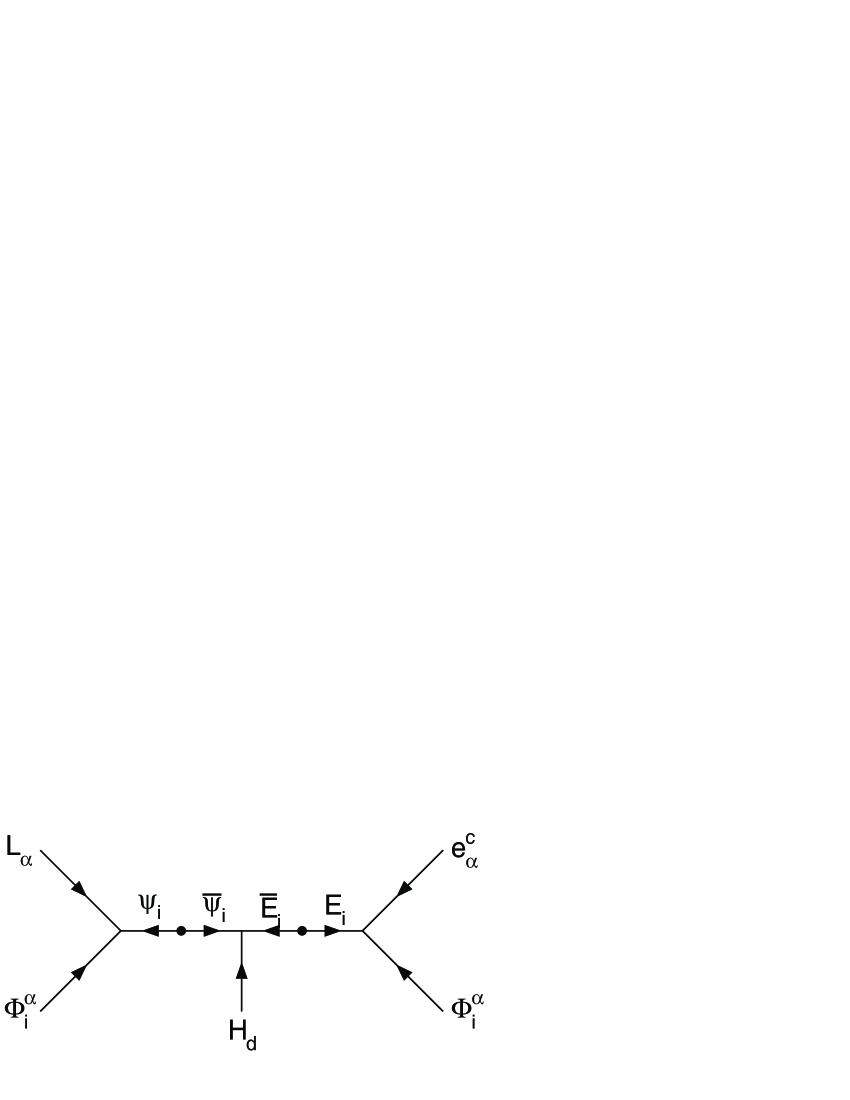
Figure 1: Effective operators inducing charged lepton masses.

Note that the mass scale $M_{i}$ in Eq. (6) is of order 5 TeV for generating realistic $\tau$–lepton mass, of order 20 TeV for the $\mu$ mass and of order 300 TeV for the electron mass (assuming that all relevant Yukawa couplings are of order one). Since these masses are all much heavier than the effective SUSY breaking scale of order 1 TeV, these heavy fields will have no effect in the low energy SUSY phenomenology within AMSB. Note that no generation mixing is induced by these effective operators, which will guarantee the approximate conservation of electron number, muon number and tau lepton number. This is what makes the model consistent with FCNC data even when $SU(3)_{H}$ is broken at the TeV scale. Since the Higgs potential respects $SU(3)_{H}\otimes SU(3)_{G}$ symmetry, after spontaneous symmetry breaking, the diagonal subgroup $SU(3)_{G+H}$ remains as an unbroken global symmetry. This subgroup contains $e$, $\mu$ and $\tau$ lepton numbers.

Since right–handed neutrinos are not required to be light for $SU(3)_{H}$ anomaly cancellation, they acquire heavy masses and decouple from the low energy theory. Small neutrino masses are then induced through the seesaw mechanism. Specifically, the following effective nonrenormalizable operators emerge after integrating out the heavy right–handed neutrino fields:

$$L^{\nu}_{eff}=\frac{\lambda_{ij}^{\alpha\beta}L_{\alpha}L_{\beta}H_{u}H_{u}\Phi^{\alpha}_{i}\Phi^{\beta}_{j}}{M_{N}^{3}}.$$ (7)

Here $M_{N}$ represents the masses of the heavy right–handed neutrino fields. For $M_{N}\sim 10^{7}$ GeV and $\left\langle\Phi_{i}\right\rangle\sim$ TeV, neutrino masses in the right range for oscillation phenomenology are obtained. Note that Eq. (7) arises from integrating neutral leptons with their masses assumed to break all global symmetries. This enables generation of large neutrino mixing angles, as needed for phenomenology.

3 Symmetry Breaking

The $SU(3)_{H}$ model has two sets of Higgs bosons: the usual MSSM Higgs doublets $H_{u}$ and $H_{d}$, and the $SU(3)_{H}$ Higgs antitriplets $\Phi_{i}\,\,\ (i=1,2,3)$. The Higgs potential is derived from the superpotential of Eq. (5) and includes the soft terms and the $D$ terms. The tree level potential splits into two pieces:

$$V(H_{u},H_{d},\Phi_{i}) = V(H_{u},H_{d})+V(\Phi_{i}),$$ (8)

enabling us to analyze them independently. The first part, $V(H_{u},H_{d})$, is identical to the MSSM potential which is well studied. There are however significant constraints on the parameters in our AMSB extension, which we now discuss.

3.1 Constraints on $\tan{\beta}$ and $m_{h}$

Minimization of $V(H_{u},H_{d})$ gives

$$\sin{2\beta}=\frac{-2B\mu}{2\mu^{2}+m_{H_{u}}^{2}+m_{H_{d}}^{2}},\,\,\,\ \mu^{2}=\frac{m_{H_{d}}^{2}-m_{H_{u}}^{2}\tan^{2}{\beta}}{\tan^{2}{\beta}-1}-\frac{M_{Z}^{2}}{2}.$$ (9)

Here $m_{H_{u}}^{2}$ and $m_{H_{d}}^{2}$ are the Higgs soft masses and are given in the Appendix for the AMSB model (see Eqs. (58)–(59).) The constraints on $m_{h}$ and $\tan{\beta}$ arise since these soft masses and the $B$ parameter are determined in terms of a single parameter $M_{aux}$ in our framework.

We eliminate $M_{aux}$ in favor of $M_{2}$, the Wino mass ($M_{2}=\frac{b_{2}g^{2}_{2}}{16\pi^{2}}M_{aux}$). We see from Eqs. (9), (4) as well as from Eqs. (45)–(46) and Eqs. (58)–(59) of the Appendix that $\tan{\beta}$ is fixed in terms of $M_{2}$. In Fig. 2 we plot $\tan{\beta}$ as a function of $M_{2}$. For the experimentally interesting range of $M_{2}\gtrsim$ 100 GeV, we find that $\tan{\beta}\simeq$ 3.8 – 4.0. In obtaining the limit on $\tan{\beta}$, we followed the following procedure. As inputs at $M_{Z}$ we chose [17]

$$\alpha_{3}(M_{Z})=0.119,\,\,\,\,\sin^{2}{\theta_{W}}=0.2312,\,\,\,\,\alpha(M_{Z})=\frac{1}{127.9}.$$ (10)

Using the central value of $M_{t}=174.3$ GeV, we obtain the running mass $m_{t}(M_{t})$ with the 2–loop QCD correction as [18]

$$\frac{M_{t}}{m_{t}(M_{t})}=1+\frac{4}{3}\frac{\alpha_{3}(M_{t})}{\pi}+10.9\left(\frac{\alpha_{3}(M_{t})}{\pi}\right)^{2}.$$ (11)

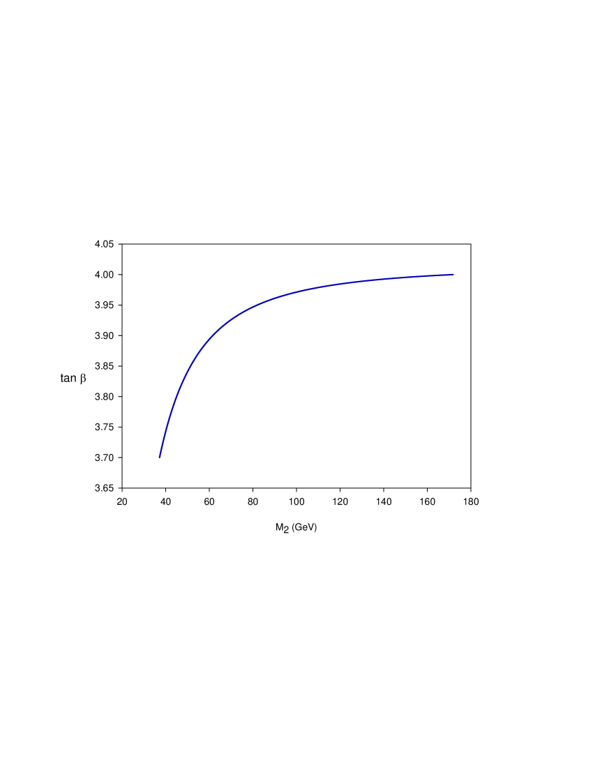
Figure 2: Plot of $\tan{\beta}$ as a function of $M_{2}$

Using 5–flavor SM QCD beta functions we extrapolated $\alpha_{3}(M_{Z})$ and obtained $\alpha_{3}(M_{t})$ = 0.109. The top quark Yukawa coupling is then found to be (for $M_{t}$ = 174.3 GeV) $Y^{SM}_{t}(M_{t})$ = 0.935 corresponding to $m_{t}(M_{t})=162.8$ GeV. This coupling is then evolved from $M_{t}$ to 1 TeV where we minimize the MSSM Higgs potential. Using standard model beta function we obtain $Y^{SM}_{t}(1$ TeV$)$ = 0.851. The corresponding MSSM coupling is $Y_{t}(1$ TeV$)=Y^{SM}_{t}(1$ TeV$)/\sin{\beta}$ , which for $\tan{\beta}\simeq 4.0$ (justified a–posteriori) is $Y_{t}(1$ TeV$)=0.824$. The gauge couplings at 1 TeV are found to be $g_{1}(1$ TeV$)=0.466,\,\,\,\,g_{2}(1$ TeV$)=0.642\,\,\,\,$and$\,\,\,\,g_{3}(1$ TeV$)=1.098$. With these values of couplings at 1 TeV we obtained Fig. 1. Uncertainties in the prediction for $\tan{\beta}$ are estimated to be $\pm 0.5$, arising from the error in top quark mass and from the precise scale at which the Higgs potential is minimized. We conclude that $\tan{\beta}$ = 3.5–4.5 in this model.

Since $\tan{\beta}$ is fixed and since the $A_{t}$ parameter is not free in AMSB, there is a nontrivial prediction for the lightest Higgs boson mass $m_{h}$. We use the 2–loop radiatively corrected expression for $m^{2}_{h}=(m^{2}_{h})_{o}+\Delta m_{h}^{2}$, where $(m^{2}_{h})_{o}$ is the tree–level value of the mass and the radiative correction is given by [19]

$$\Delta m_{h}^{2} = \frac{3m_{t}^{4}}{4\pi^{2}\upsilon^{2}}\left[t+X_{t}+\frac{1}{16\pi^{2}}\left(\frac{3}{2}\frac{m_{t}^{2}}{\upsilon^{2}}-32\pi\alpha_{3}(M_{t})\right)(2X_{t}t+t^{2})\right].$$ (12)

Here

$$X_{t}=\frac{\tilde{A_{t}}^{2}}{m_{\tilde{t}}^{2}}\left(1-\frac{\tilde{A_{t}}^{2}}{12m_{\tilde{t}}^{2}}\right),\,\,\,\ \tilde{A_{t}}=A_{t}-\mu\cot{\beta},$$ (13)

and $t=$log$(\frac{m_{\tilde{t}}^{2}}{M_{t}^{2}})$, $\upsilon=174$ GeV. $m_{\tilde{t}}^{2}$ is the arithmetic average of the diagonal entries of the squared stop mass matrix and $A_{t}$ is the soft trilinear coupling associated with the top Yukawa coupling in the superpotential of Eq. (5). In these expressions, $m_{t}$ is the one–loop QCD corrected running mass, $m_{t}=\frac{M_{t}}{1+\frac{4}{3}\frac{\alpha_{3}(M_{t})}{\pi}}$, which equals 166.7 GeV for $M_{t}=174.3$ GeV. We find that $m_{h}\simeq$ 113 GeV – 120 GeV, depending on the choice of $M_{aux}$. The larger value $m_{h}\simeq 120$ GeV is realized only for larger $M_{t}\simeq 180$ GeV. We list in Tables 2–4 the value of $m_{h}$, along with the other sparticle masses.

3.2 $SU(3)_{H}$ symmetry breaking

Let us now analyze the $SU(3)_{H}$ symmetry breaking sector of the potential. The potential $V(\Phi_{i})$ is given by:

$$V(\Phi_{i}) = m_{\phi}^{2}(\Phi_{1}^{{\dagger}}\Phi_{1}+\Phi_{2}^{{\dagger}}\Phi_{2}+\Phi_{3}^{{\dagger}}\Phi_{3})+\kappa A_{\kappa}\left(\Phi_{1}^{\alpha}\Phi_{2}^{\beta}\Phi_{3}^{\gamma}\epsilon_{\alpha\beta\gamma}+c.c\right)$$ (14)

$$+ \kappa^{2}\left[(\Phi_{1}\Phi_{2})^{{\dagger}}(\Phi_{1}\Phi_{2})+(\Phi_{1}\Phi_{3})^{{\dagger}}(\Phi_{1}\Phi_{3})+(\Phi_{2}\Phi_{3})^{{\dagger}}(\Phi_{2}\Phi_{3})\right]$$

$$+ \frac{g_{4}^{2}}{8}\sum_{a=1}^{8}|\Phi_{1}^{{\dagger}}\lambda^{a}\Phi_{1}+\Phi_{2}^{{\dagger}}\lambda^{a}\Phi_{2}+\Phi_{3}^{{\dagger}}\lambda^{a}\Phi_{3}|^{2}.$$

Here $g_{4}$ is the gauge coupling of the $SU(3)_{H}$, $A_{\kappa}$ is the trilinear $A$–term corresponding to the coupling $\kappa$, $m^{2}_{\phi}$ is the soft mass squared for the $\Phi_{i}$ fields. These soft SUSY breaking parameters are given in the Appendix (Eqs. (56), (60)). The $\kappa^{2}$ term in Eq. (14) is the $F$-term contribution and the last term in Eq. (14) is the $SU(3)_{H}$ $D$–term with $\lambda^{a}$ being the $SU(3)_{H}$ generators.

The Higgs potential, Eq. (14), has an $SU(3)_{H}\times SU(3)_{G}$ symmetry, with the $\Phi_{i}$ fields $(i=1-3)$ transforming as $\bf{(\bar{3},3)}$. This allows for a vacuum which preserves an $SU(3)_{H+G}$ diagonal subgroup. The VEVs of the $\Phi_{i}$ fields are then given by:

$$\left\langle\Phi_{1}\right\rangle=\pmatrix{u\cr 0\cr 0},\qquad\qquad\left\langle\Phi_{2}\right\rangle=\pmatrix{0\cr u\cr 0}\qquad\mbox{and}\qquad\left\langle\Phi_{3}\right\rangle=\pmatrix{0\cr 0\cr u}.$$ (15)

Using these VEVs the potential becomes

$$\left\langle V(\Phi)\right\rangle = 3m_{\phi}^{2}u^{2}+3\kappa^{2}u^{4}+2\kappa A_{\kappa}u^{3}.$$ (16)

Minimization of Eq. (16) leads to the condition

$$u = \frac{-A_{\kappa}\pm\sqrt{-8m_{\phi}^{2}+A_{\kappa}^{2}}}{4\kappa}.$$ (17)

The argument in the square root of Eq. (17), which should be positive for a consistent symmetry breaking, is given by

$$-8m_{\phi}^{2}+A_{\kappa}^{2} = \frac{M_{aux}^{2}}{(16\pi^{2})^{2}}[15\kappa^{4}+56\kappa^{2}\lambda^{2}+304\lambda^{4}-8\kappa^{2}g_{4}^{2}-32\lambda^{2}g_{4}^{2}].$$ (18)

Positivity of Eq. (18) leads to constraints on the parameters $\{\lambda,\,\,\kappa\}$. It can be shown that Eq. (18) implies $0\leqslant|\kappa|\leqslant 0.731g_{4}$ and $0\leqslant|\lambda|\leqslant 0.324g_{4}$. Furthermore, positivity of the slepton masses, along with the experimental limit $m^{2}_{slepton}\gtrsim(100$ GeV$)^{2}$, require $g_{4}\geqslant 0.5$. This essentially fixes the parameter space of the model. We get the right minimum by choosing the negative sign of the square root in Eq. (17) (for positive $M_{aux}$), with this choice, all the Higgs masses–squared will be positive.

Since the symmetry breaking chain is $SU(3)_{H}\times SU(3)_{G}\rightarrow SU(3)_{H+G}$, we can classify the masses of all scalars and fermions as multiplets of $SU(3)_{H+G}$. The complex $\Phi(\bar{3},3)$ scalar multiplet decomposes into 2 octets and two singlets of $SU(3)_{H+G}$. One octet gets eaten by the Higgs mechanism. A physical octet remains in the spectrum with a mass given by

$$\mathcal{M}^{2}_{octet} = -2\kappa^{2}u^{2}-2\kappa uA_{\kappa}+g_{4}^{2}u^{2}.$$ (19)

There are two singlets, one scalar ($\phi_{s}$) and one pseudoscalar ($\phi_{p}$) with masses given by

$$m^{2}_{\phi_{s}} = 4\kappa^{2}u^{2}+\kappa uA_{\kappa},$$ (20)

$$m^{2}_{\phi_{p}} = -3\kappa uA_{\kappa}.$$ (21)

In the fermionic sector, the octet Higgsino mixes with the octet gaugino with a mixing matrix given by

$$\mathcal{M}_{octet}^{{}^{\prime}} = \pmatrix{m_{4}&g_{4}u\cr g_{4}u&\kappa u}.$$ (22)

In addition, there is a Majorana fermion, a singlet of $SU(3)_{H+G}$, with a mass of

$$m_{\tilde{{\phi}}} = 2\kappa u.$$ (23)

Finally the gauge bosons form an octet with a mass

$$M_{V}=g_{4}u.$$ (24)

4 The SUSY Spectrum

We are now ready to discuss the full SUSY spectrum of the model. We will see that the tachyonic slepton problem is cured by virtue of the positive contribution from the $SU(3)_{H}$ gauge sector.

4.1 Slepton masses

The slepton mass–squareds are given by the eigenvalues of the mass matrices ($\alpha=e,\,\mu,\,\tau$)

$$M^{2}_{\tilde{l}}=\pmatrix{m^{2}_{\tilde{L}_{\alpha}}&m_{E_{\alpha}}\left(A_{Y_{E_{\alpha}}}-\mu\tan{\beta}\right)\cr m_{E_{\alpha}}\left(A_{Y_{E_{\alpha}}}-\mu\tan{\beta}\right)&m^{2}_{\tilde{e}^{c}_{\alpha}}}.$$ (25)

Here

$$m^{2}_{\tilde{L}_{\alpha}} = \frac{M_{aux}^{2}}{(16\pi^{2})}\left[Y_{E_{\alpha}}\beta(Y_{E_{\alpha}})-\left(\frac{3}{2}g_{2}\beta(g_{2})+\frac{3}{10}g_{1}\beta(g_{1})+\frac{8}{3}g_{4}\beta(g_{4})\right)\right]$$ (26)

$$+ m_{E_{\alpha}}^{2}+\left(-\frac{1}{2}+\sin^{2}{\theta_{W}}\right)\cos{2\beta}M_{Z}^{2},$$

$$m^{2}_{\tilde{e}^{c}_{\alpha}} = \frac{M_{aux}^{2}}{(16\pi^{2})}\left[2Y_{E_{\alpha}}\beta(Y_{E_{\alpha}})-\left(\frac{6}{5}g_{1}\beta(g_{1})+\frac{8}{3}g_{4}\beta(g_{4})\right)\right]$$ (27)

$$+ m_{E_{\alpha}}^{2}-\sin^{2}{\theta_{W}}\cos{2\beta}M_{Z}^{2}.$$

The off diagonal terms in Eq. (25) are rather small as they are proportional to the lepton masses. The SUSY soft masses are calculated from the RGE give in the Appendix. The last terms of Eqs. (26)–(27) are the $D$–terms. Note the positive contribution from the $SU(3)_{H}$ gauge sector in Eqs. (26)–(27), given by the term $-\frac{8}{3}g_{4}\beta(g_{4})$. In our model $g_{4}$ is asymptotically free with $\beta(g_{4})=-\frac{3}{16\pi^{2}}g_{4}^{3}$. This contribution makes the mass–squared of all sleptons to be positive for $g_{4}\geqslant 0.5$.

4.2 Squark masses

The mixing matrix for the squark sector is similar to the slepton sector. The diagonal entries of the up and the down squark mass matrices are given by [20]

$$m_{\tilde{U}_{i}}^{2} = (m^{2}_{soft})_{\tilde{Q}_{i}}^{\tilde{Q}_{i}}+m_{U_{i}}^{2}+\frac{1}{6}\left(4M_{W}^{2}-M_{Z}^{2}\right)\cos{2\beta},$$

$$m_{\tilde{U}^{c}_{i}}^{2} = (m^{2}_{soft})_{\tilde{U}_{i}^{c}}^{\tilde{U}_{i}^{c}}+m_{U_{i}}^{2}-\frac{2}{3}\left(M_{W}^{2}-M_{Z}^{2}\right)\cos{2\beta},$$

$$m_{\tilde{D}_{i}}^{2} = (m^{2}_{soft})_{\tilde{Q}_{i}}^{\tilde{Q}_{i}}+m_{D_{i}}^{2}-\frac{1}{6}\left(2M_{W}^{2}+M_{Z}^{2}\right)\cos{2\beta},$$

$$m_{\tilde{D}_{i}^{c}}^{2} = (m^{2}_{soft})_{\tilde{D}_{i}^{c}}^{\tilde{D}_{i}^{c}}+m_{D_{i}}^{2}+\frac{1}{3}\left(M_{W}^{2}-M_{Z}^{2}\right)\cos{2\beta}.$$ (28)

Here $m_{U_{i}}$ and $m_{D_{i}}$ are quark masses of different generations, $i$ = 1, 2, 3. The squark soft masses are obtained from the RGE as

$$(m^{2}_{soft})_{\tilde{Q}_{i}}^{\tilde{Q}_{i}}=\frac{M_{aux}^{2}}{16\pi^{2}}\left(Y_{u_{i}}\beta{(Y_{u_{i}})}+Y_{d_{i}}\beta{(Y_{d_{i}})}-\frac{1}{30}g_{1}\beta{(g_{1})}-\frac{3}{2}g_{2}\beta{(g_{2})}-\frac{8}{3}g_{3}\beta{(g_{3})}\right),$$ (29)

$$(m^{2}_{soft})_{\tilde{U}_{i}^{c}}^{\tilde{U}_{i}^{c}} = \frac{M_{aux}^{2}}{16\pi^{2}}\left(2Y_{u_{i}}\beta{(Y_{u_{i}})}-\frac{8}{15}g_{1}\beta{(g_{1})}-\frac{8}{3}g_{3}\beta{(g_{3})}\right),$$ (30)

$$(m^{2}_{soft})_{\tilde{D}_{i}^{c}}^{\tilde{D}_{i}^{c}} = \frac{M_{aux}^{2}}{16\pi^{2}}\left(2Y_{d_{i}}\beta{(Y_{d_{i}})}-\frac{2}{15}g_{1}\beta{(g_{1})}-\frac{8}{3}g_{3}\beta{(g_{3})}\right).$$ (31)

4.3 $\eta$ fermion and $\eta$ scalar masses

The fields $\eta$ and $\bar{\eta}$ transform as $(3,\bar{3})$ and $(\bar{3},3)$ under $SU(3)_{H}\times SU(3)_{G}$. After symmetry breaking, $\eta$ and $\bar{\eta}$ both transform as ${\bf 8+1}$ of the diagonal $SU(3)_{H+G}$. The octet from $\eta$ mixes with the octet from $\bar{\eta}$, and similarly for the singlets.

In the fermionic sector, the octet and the singlet mass matrices are given by

$$M_{octet}^{\eta}=\pmatrix{-2\lambda u&M_{\eta}\cr M_{\eta}&0},$$ (32)

$$M_{singlet}^{\eta}=\pmatrix{4\lambda u&M_{\eta}\cr M_{\eta}&0}.$$ (33)

In the scalar sector, there are 4 real octets and 4 real singlets from $\eta$ and $\bar{\eta}$ fields. The two scalar octets are mixed, as are the two pseudoscalar octets. The mass squared matrices for the octet are

$$M^{2}_{s-octet} = \pmatrix{(\tilde{m}^{2}_{soft})_{\eta}^{\eta}+M_{\eta}^{2}+2\lambda u(-A_{\lambda}-\kappa u+2\lambda u)&M_{\eta}(B_{\eta}-2\lambda u)\cr M_{\eta}(B_{\eta}-2\lambda u)&(\tilde{m}^{2}_{soft})_{\bar{\eta}}^{\bar{\eta}}+M_{\eta}^{2}},$$ (34)

$$M^{2}_{p-octet} = \pmatrix{(\tilde{m}^{2}_{soft})_{\eta}^{\eta}+M_{\eta}^{2}+2\lambda u(A_{\lambda}+\kappa u+2\lambda u)&-M_{\eta}(B_{\eta}+2\lambda u)\cr-M_{\eta}(B_{\eta}+2\lambda u)&(\tilde{m}^{2}_{soft})_{\bar{\eta}}^{\bar{\eta}}+M_{\eta}^{2}}.$$ (35)

The singlet scalar mass matrices are

$$M^{2}_{s-singlet} = \pmatrix{(\tilde{m}^{2}_{soft})_{\eta}^{\eta}+M_{\eta}^{2}+4\lambda u(A_{\lambda}+\kappa u+4\lambda u)&M_{\eta}(B_{\eta}+4\lambda u)\cr M_{\eta}(B_{\eta}+4\lambda u)&(\tilde{m}^{2}_{soft})_{\bar{\eta}}^{\bar{\eta}}+M_{\eta}^{2}},$$ (36)

$$M^{2}_{p-singlet} = \pmatrix{(\tilde{m}^{2}_{soft})_{\eta}^{\eta}+M_{\eta}^{2}-4\lambda u(A_{\lambda}-\kappa u-4\lambda u)&-M_{\eta}(B_{\eta}-4\lambda u)\cr-M_{\eta}(B_{\eta}-4\lambda u)&(\tilde{m}^{2}_{soft})_{\bar{\eta}}^{\bar{\eta}}+M_{\eta}^{2}}.$$ (37)

The soft masses $(\tilde{m}^{2}_{soft})_{\eta}^{\eta}$ and $(\tilde{m}^{2}_{soft})_{\eta}^{\eta}$ are given in Eqs. (61)–(62) of the Appendix.

5 Numerical Results

We are now ready to present our numerical results for the SUSY spectrum. The scale of SUSY breaking, $M_{aux}$, should be in the range 40–120 TeV for the MSSM particles to have masses in the range 100 GeV – 2 TeV. Note that there is a large hierarchy in the masses of the gluino and the neutral Wino, $\frac{M_{3}}{M_{2}}\simeq 7.1$ (after taking account of radiative corrections), in AMSB models. Furthermore the lightest chargino is nearly mass degenerate with the neutral Wino, so $M_{2}\gtrsim 100$ GeV is required to satisfy the LEP chargino mass bound.

The $SU(3)_{H}$ gauge coupling $g_{4}$ is chosen so that the sleptons have positive mass squared ($g_{4}\geqslant 0.5$). We allow $g_{4}$ to take two values, $g_{4}$ = 0.55 (Tables 2 and 4) and $g_{4}$ = 1.0 (Table 3). Symmetry breaking considerations constrain the couplings $\kappa$ and $\lambda$ as discussed in Sec. 3 after Eq. (18). In Tables 2 and 4 we have taken $M_{aux}$ = 47.112 TeV corresponding to a light spectrum, while in Table 3 we have $M_{aux}$ = 66.695 TeV with an intermediate spectrum. Other input parameters are listed in the respective Table captions. The mass parameter $M_{\eta}$ cannot be much larger than 1 TeV, as that would decouple the effects of $\eta$, $\bar{\eta}$ fields which are needed for consistent symmetry breaking.

We see from Table 2 that the lightest Higgs boson mass is $m_{h}\simeq 113$ GeV. This is very close to the current experimental limit. If $M_{t}$ = 180 GeV is used (instead of $M_{t}$ = 176 GeV), for the same set of input parameters, $m_{h}$ will be 115 GeV. $m_{h}$ being close to the current experimental limit is a generic prediction of our framework. It holds in the spectra of Tables 3 and 4 as well. We conclude that $m_{h}\lesssim 120$ GeV in this model.

The masses of the sleptons will depend sensitively on the choice of $g_{4}$. The sleptons are relatively light, $m_{slep}\lesssim$ 300 GeV, with $g_{4}=0.55$, while they are heavy, $m_{slep}\simeq$ 800 GeV, when $g_{4}=1.0$. Note however that there is a correlation in the slepton masses and the $SU(3)_{H}$ gauge boson masses ($M_{V}$), with the lighter sleptons corresponding to lighter $SU(3)_{H}$ gauge bosons. It is worth noting that very light sleptons, below the current experimental limits of about 100 GeV, would be inconsistent with the limits on $M_{V}$ arising from $e^{+}e^{-}\rightarrow\mu^{+}\mu^{-}$ type processes (see Sec. 6). Note also that the left–handed and the right–handed sleptons are nearly degenerate to within about 10 GeV in this model. This a numerical coincidence having to do with the values of $g_{1}$ and $g_{2}$ and the MSSM beta functions (see the last paper of Ref. [5]). The new $SU(3)_{H}$ gauge boson contributions to the slepton masses are the same for the left–handed and the right–handed sleptons.

In Tables 2–4 we have included the leading radiative corrections to the gaugino masses $M_{1}$, $M_{2}$ and $M_{3}$ [21]. Including these radiative corrections we find (in Table 2) $M_{1}:M_{2}:M_{3}=2.9:1:7.3$. The lightest SUSY particle (LSP) is the neutral Wino, which is nearly mass degenerate with the charged Wino. In Tables 2–4 the mass splitting is about 60 MeV, but this does not take into account $SU(2)_{L}\times U(1)_{Y}$ breaking corrections [22]. These electroweak radiative corrections turn out to be very important, and we find $m_{\chi^{\pm}_{1}}-m_{\chi_{1}^{0}}\simeq 235$ MeV (with about 175 MeV arising from $SU(2)_{L}\times U(1)_{Y}$ breaking effects). The decay $\chi_{1}^{\pm}\rightarrow\chi_{1}^{0}+\pi^{\pm}$ is then kinematically allowed, with the $\pi^{\pm}$ being very soft. Once produced, the neutralino $\chi_{1}^{0}$ will escape the detector without leaving any tracks. With the decay channel $\chi_{1}^{\pm}\rightarrow\chi_{1}^{0}+\pi^{\pm}$ open, the lightest chargino will leave an observable track with a decay length of about a few cm. Search strategies for such a quasi–degenerate pair at colliders have been analyzed in Ref. [21, 23, 24].

In the $SU(3)_{H}$ sector, in Tables 2–4, the horizontal gauge boson has a mass of 1.5–4.0 TeV. The heavy Higgs bosons, Higgsinos, gauginos, squarks and the $\eta$ fields all have masses $\lesssim(1-2)$ TeV.

MSSM Particles	Symbol	Mass (TeV)
Neutralinos	$\{m_{\tilde{\chi}_{1}^{0}},\,\,m_{\tilde{\chi}_{2}^{0}},\,\,m_{\tilde{\chi}_{3}^{0}},\,\,m_{\tilde{\chi}_{4}^{0}}\}$	$\{0.14158,\,\,0.429,\,\,0.872,\,\,0.879\}$
Charginos	$\{m_{\tilde{\chi}_{1}^{\pm}},\,\,m_{\tilde{\chi}_{2}^{\pm}}\}$	$\{0.14164,\,\,0.878\}$
Gluino	$M_{3}$	$1.065$
Higgs bosons	$\{m_{h},\,\,m_{H},\,\,m_{A},\,\,m_{H^{\pm}}\}$	$\{0.113,\,\,0.897,\,\,0.896,\,\,0.900\}$
R.H sleptons	$\{m_{\tilde{e}_{R}},\,\,m_{\tilde{\mu}_{R}},\,\,m_{\tilde{\tau}_{1}}\}$	$\{0.183,\,\,0.183,\,\,0.170\}$
L.H sleptons	$\{m_{\tilde{e}_{L}},\,\,m_{\tilde{\mu}_{L}},\,\,m_{\tilde{\tau}_{2}}\}$	$\{0.190,\,\,0.190,\,\,0.200\}$
Sneutrinos	$\{m_{\tilde{\nu}_{e}},\,\,m_{\tilde{\nu}_{\mu}},\,\,m_{\tilde{\nu}_{\tau}}\}$	$\{0.175,\,\,0.175,\,\,0.175\}$
R.H down squarks	$\{m_{\tilde{d}_{R}},\,\,m_{\tilde{s}_{R}},\,\,m_{\tilde{b}_{1}}\}$	$\{1.017,\,\,1.017,\,\,1.014\}$
L.H down squarks	$\{m_{\tilde{d}_{L}},\,\,m_{\tilde{s}_{L}},\,\,m_{\tilde{b}_{2}}\}$	$\{1.008,\,\,1.008,\,\,0.886\}$
R.H up squarks	$\{m_{\tilde{u}_{R}},\,\,m_{\tilde{c}_{R}},\,\,m_{\tilde{t}_{1}}\}$	$\{1.011,\,\,1.011,\,\,0.718\}$
L.H up squarks	$\{m_{\tilde{u}_{L}},\,\,m_{\tilde{c}_{L}},\,\,m_{\tilde{t}_{2}}\}$	$\{1.005,\,\,1.005,\,\,0.944\}$
New Particles	Symbol	Mass (TeV)
$SU(3)_{H}$ Gauge boson octet	$M_{V}$	$2.213$
Singlet Higgsino	$m_{\tilde{{\phi}}}$	$0.402$
Octet Higgsino/gaugino	$m_{\tilde{\phi}_{{1,2}}}$	$\{1.978,\,\,2.450\}$
$\phi$ Higgs bosons	$\{m_{\phi_{s}},m_{\phi_{p}},m_{\phi-octet}\}$	$\{0.179,\,\,0.624,\,\,2.253\}$
Fermionic $\eta$ (octet)	$m^{octet}_{{\eta}_{1,2}}$	$\{0.676,\,\,1.480\}$
Fermionic $\eta$ (singlet)	$m^{singlet}_{{\eta}_{1,2}}$	$\{0.479,\,\,2.089\}$
Scalar $\eta$ Higgs (octet)	$m^{s-octet}_{\tilde{\eta}_{1,2}}$	$\{0.454,\,\,1.703\}$
Pseudoscalar $\eta$ Higgs (octet)	$m^{p-octet}_{\tilde{\eta}_{1,2}}$	$\{0.908,\,\,1.259\}$
Scalar $\eta$ Higgs (singlet)	$m^{s-singlet}_{\tilde{\eta}_{1,2}}$	$\{0.717,\,\,1.868\}$
Pseudoscalar $\eta$ Higgs (singlet)	$m^{p-singlet}_{\tilde{\eta}_{1,2}}$	$\{0.264,\,\,2.310\}$

Table 2: Sparticle masses for the choice $M_{aux}=47.112$ TeV, $\tan{\beta}=3.986$, $\mu=0.870$ TeV, $y_{b}=0.0713$, $\lambda=0.1$, $\kappa=0.05$, $g_{4}=0.55$, $u=-4.024$ TeV, $M_{\eta}=1.0$ TeV and $M_{t}=0.176$ TeV.

MSSM Particles	Symbol	Mass (TeV)
Neutralinos	$\{m_{\tilde{\chi}_{1}^{0}},\,\,m_{\tilde{\chi}_{2}^{0}},\,\,m_{\tilde{\chi}_{3}^{0}},\,\,m_{\tilde{\chi}_{4}^{0}}\}$	$\{0.19625,\,\,0.585,\,\,1.179,\,\,1.184\}$
Charginos	$\{m_{\tilde{\chi}_{1}^{\pm}},\,\,m_{\tilde{\chi}_{2}^{\pm}}\}$	$\{0.196291,\,\,1.183\}$
Gluino	$M_{3}$	$1.411$
Higgs boson	$\{m_{h},\,\,m_{H},\,\,m_{A},\,\,m_{H^{\pm}}\}$	$\{0.115,\,\,1.177,\,\,1.176,\,\,1.179\}$
R.H sleptons	$\{m_{\tilde{e}_{R}},\,\,m_{\tilde{\mu}_{R}},\,\,m_{\tilde{\tau}_{1}}\}$	$\{0.245,\,\,0.245,\,\,0.232\}$
L.H sleptons	$\{m_{\tilde{e}_{L}},\,\,m_{\tilde{\mu}_{L}},\,\,m_{\tilde{\tau}_{2}}\}$	$\{0.254,\,\,0.254,\,\,0.263\}$
Sneutrinos	$\{m_{\tilde{\nu}_{e}},\,\,m_{\tilde{\nu}_{\mu}},\,\,m_{\tilde{\nu}_{\tau}}\}$	$\{0.242,\,\,0.242,\,\,0.242\}$
R.H down squarks	$\{m_{\tilde{d}_{R}},\,\,m_{\tilde{s}_{R}},\,\,m_{\tilde{b}_{1}}\}$	$\{1.373,\,\,1.373,\,\,1.369\}$
L.H down squraks	$\{m_{\tilde{d}_{L}},\,\,m_{\tilde{s}_{L}},\,\,m_{\tilde{b}_{2}}\}$	$\{1.361,\,\,1.361\,\,1.195\}$
R.H up squarks	$\{m_{\tilde{u}_{R}},\,\,m_{\tilde{c}_{R}},\,\,m_{\tilde{t}_{1}}\}$	$\{1.365,\,\,1.365,\,\,0.983\}$
L.H up squraks	$\{m_{\tilde{u}_{L}},\,\,m_{\tilde{c}_{L}},\,\,m_{\tilde{t}_{2}}\}$	$\{1.359\,\,1.359,\,\,1.244\}$
New Particles	Symbol	Mass (TeV)
$SU(3)_{H}$ Gauge boson octet	$M_{V}$	$1.871$
Singlet Higgsino	$m_{\tilde{{\phi}}}$	$0.544$
Octet Higgsino/gaugino	$m_{\tilde{\phi}_{{1,2}}}$	$\{1.553,\,\,2.191\}$
$\phi$ Higgs bosons	$\{m_{\phi_{s}},m_{\phi_{p}},m_{\phi-octet}\}$	$\{0.247,\,\,0.840,\,\,1.955\}$
Fermionic $\eta$ (octet)	$m^{octet}_{{\eta}_{1,2}}$	$\{0.716,\,\,1.397\}$
Fermionic $\eta$ (singlet)	$m^{singlet}_{{\eta}_{1,2}}$	$\{0.529,\,\,1.890\}$
Scalar $\eta$ Higgs (octet)	$m^{s-octet}_{\tilde{\eta}_{1,2}}$	$\{0.421,\,\,1.699\}$
Pseudoscalar $\eta$ Higgs (octet)	$m^{p-octet}_{\tilde{\eta}_{1,2}}$	$\{1.031,\,\,1.098\}$
Scalar $\eta$ Higgs (singlet)	$m^{s-singlet}_{\tilde{\eta}_{1,2}}$	$\{0.850,\,\,1.593\}$
Pseudoscalar $\eta$ Higgs (singlet)	$m^{p-singlet}_{\tilde{\eta}_{1,2}}$	$\{0.247,\,\,2.189\}$

Table 3: Sparticle masses for the choice $M_{aux}=63.695$ TeV, $\tan{\beta}=3.999$, $\mu=1.177$ TeV, $y_{b}=0.0716$, $\lambda=0.1$, $\kappa=0.08$, $g_{4}=0.55$, $u=-3.402$ TeV, $M_{\eta}=1.0$ TeV and $M_{t}=0.1743$ TeV.

MSSM Particles	Symbol	Mass (TeV)
Neutralinos	$\{m_{\tilde{\chi}_{1}^{0}},\,\,m_{\tilde{\chi}_{2}^{0}},\,\,m_{\tilde{\chi}_{3}^{0}},\,\,m_{\tilde{\chi}_{4}^{0}}\}$	$\{0.143,\,\,0.434,\,\,0.872,\,\,0.879\}$
Charginos	$\{m_{\tilde{\chi}_{1}^{\pm}},\,\,m_{\tilde{\chi}_{2}^{\pm}}\}$	$\{0.143219,\,\,0.878\}$
Gluino	$M_{3}$	$1.065$
Higgs boson	$\{m_{h},\,\,m_{H},\,\,m_{A},\,\,m_{H^{\pm}}\}$	$\{0.113,\,\,0.897,\,\,0.896,\,\,0.900\}$
R.H sleptons	$\{m_{\tilde{e}_{R}},\,\,m_{\tilde{\mu}_{R}},\,\,m_{\tilde{\tau}_{1}}\}$	$\{0.825,\,\,825,\,\,0.823\}$
L.H sleptons	$\{m_{\tilde{e}_{L}},\,\,m_{\tilde{\mu}_{L}},\,\,m_{\tilde{\tau}_{2}}\}$	$\{0.827,\,\,0.827,\,\,0.828\}$
Sneutrinos	$\{m_{\tilde{\nu}_{e}},\,\,m_{\tilde{\nu}_{\mu}},\,\,m_{\tilde{\nu}_{\tau}}\}$	$\{0.823,\,\,0.823,\,\,0.823\}$
R.H down squarks	$\{m_{\tilde{d}_{R}},\,\,m_{\tilde{s}_{R}},\,\,m_{\tilde{b}_{1}}\}$	$\{1.017,\,\,1.017,\,\,1.014\}$
L.H down squraks	$\{m_{\tilde{d}_{L}},\,\,m_{\tilde{s}_{L}},\,\,m_{\tilde{b}_{2}}\}$	$\{1.008,\,\,1.008,\,\,0.886\}$
R.H up squarks	$\{m_{\tilde{u}_{R}},\,\,m_{\tilde{c}_{R}},\,\,m_{\tilde{t}_{1}}\}$	$\{1.011,\,\,1.011,\,\,0.718\}$
L.H up squraks	$\{m_{\tilde{u}_{L}},\,\,m_{\tilde{c}_{L}},\,\,m_{\tilde{t}_{2}}\}$	$\{1.005,\,\,1.005,\,\,0.944\}$
New Particles	Symbol	Mass (TeV)
$SU(3)_{H}$Gauge boson octet	$M_{V}$	$3.779$
Singlet Higgsino	$m_{\tilde{{\phi}}}$	$1.058$
Octet Higgsino/gaugino	$m_{\tilde{\phi}_{{1,2}}}$	$\{3.071,\,\,4.495\}$
$\phi$ Higgs bosons	$\{m_{\phi_{s}},m_{\phi_{p}},m_{\phi-octet}\}$	$\{0.465,\,\,1.646,\,\,3.940\}$
Fermionic $\eta$ (octet)	$m^{octet}_{{\eta}_{1,2}}$	$\{0.254,\,\,2.521\}$
Fermionic $\eta$ (singlet)	$m^{singlet}_{{\eta}_{1,2}}$	$\{0.137,\,\,4.672\}$
Scalar $\eta$ Higgs (octet)	$m^{s-octet}_{\tilde{\eta}_{1,2}}$	$\{0.588,\,\,3.090\}$
Pseudoscalar $\eta$ Higgs (octet)	$m^{p-0ctet}_{\tilde{\eta}_{1,2}}$	$\{1.058,\,\,1.952\}$
Scalar $\eta$ Higgs (singlet)	$m^{s-singlet}_{\tilde{\eta}_{1,2}}$	$\{0.964,\,\,4.116\}$
Pseudoscalar $\eta$ Higgs (singlet)	$m^{p-singlet}_{\tilde{\eta}_{1,2}}$	$\{0.711,\,\,5.224\}$

Table 4: Sparticle masses for the choice $M_{aux}=47.112$ TeV, $\tan{\beta}=3.986$, $\mu=0.870$ TeV, $y_{b}=0.0713$, $\lambda=0.3$, $\kappa=0.14$, $g_{4}=1.0$, $u=-3.779$ TeV, $M_{\eta}=0.800$ TeV and $M_{t}=0.176$ TeV.

6 Experimental Signatures

The Lightest SUSY particle in the model is the neutral Wino ($\chi_{1}^{0}$) which is nearly mass degenerate with the lightest chargino ($\chi_{1}^{\pm}$), with a mass splitting of about 235 MeV. At the Tevatron Run 2 as well as at the LHC, the process $p\bar{p}\,\,(or\,\,pp)\rightarrow\chi_{1}^{0}+\chi_{1}^{\pm}$ will produce these SUSY particles. Naturalness suggest that $m_{\chi_{1}^{0}}$, $m_{\chi_{1}^{\pm}}$ $\lesssim$ 300 GeV (corresponding to $m_{gluino}\lesssim 2$ TeV). Strategies for detecting such a quasi–degenerate pair has been carried out in Ref. [21, 23, 24]. In the MSSM sector our model predicts $\tan{\beta}\simeq 4.0$ and $m_{h}\lesssim 120$ GeV, both of which can be tested at the LHC.

If the $SU(3)_{H}$ gauge coupling $g_{4}$ takes small values ($g_{4}\simeq 0.55$), the slepton masses will be near the current experimental limit. For larger values of $g_{4}$ ($\simeq 1.0$) the slepton masses are comparable to those of the squarks.

The $SU(3)_{H}$ gauge boson masses are in the range $M_{V}=1.5-4.0$ TeV. Although relatively light, these particles do not mediate leptonic FCNC, owing to the approximate $SU(3)_{H+G}$ global symmetries present in the model.

The most stringent constraint on $M_{V}$ arises from the process $e^{+}e^{-}\rightarrow\mu^{+}\mu^{-}$. LEP II has set severe constraints on lepton compositeness [25, 17] from this process. We focus on one such amplitude, involving all left–handed lepton fields. In our model, the effective Lagrangian for this process is

$$\textit{L}^{\rm eff}=-\frac{2g_{4}^{2}}{3M_{V}^{2}}(\bar{e_{L}}\gamma_{\mu}e_{L})(\bar{\mu_{L}}\gamma^{\mu}\mu_{L}).$$ (38)

Comparing with $\Lambda_{LL}^{-}(ee\mu\mu)>6.3$ TeV [17], we obtain $\frac{M_{V}}{g_{4}}\geq 2.05$ TeV. For $g_{4}=0.55~{}(1.0)$ this implies $M_{V}\geqslant$ 1.129 (2.052) TeV. From Tables 2–4 we find that these constraints are satisfied.

The model as it stands has an unbroken $Z_{2}$ symmetry (in addition to the usual $R$–parity) under which the superfields $\eta,\bar{\eta}$ are odd and all other superfields are even. If this symmetry is exact, the lightest of the $\eta$ and $\bar{\eta}$ fields (a pseudoscalar singlet Higgs in the fits of Tables 2-3 and a singlet fermion in Table 4) will be stable. We envision this $Z_{2}$ symmetry to be broken by higher dimensional terms of the type $L_{\alpha}H_{u}\Phi^{\alpha}\bar{\eta}_{\beta}\Phi^{\beta}/\Lambda^{2}$. Such a term will induce the decay $\eta_{1}^{p-singlet}\rightarrow L+\chi_{1}^{0}$ with a lifetime less than 1 second for $\Lambda\leq 10^{9}$ GeV. This would make these $\eta$ particles cosmologically safe. It may be pointed out that the same effective operator, along with a TeV scale mass for the $\eta$ fields, can provide small neutrino masses even in the absence of the operators given in Eq. (7).

7 Origin of the $\mu$ term

Any satisfactory SUSY breaking model should also have a natural explanation for the $\mu$ term (the coefficient of $H_{u}H_{d}$ term in Eq. (5)). In gravity mediated SUSY breaking models, there are at least three solutions to the $\mu$ problem. The Giudice–Masiero mechanism [26] which explains the $\mu$ term through the Kahler potential $\int H_{u}H_{d}Z^{*}d^{4}\theta/M_{pl}$ is not readily adaptable to the AMSB framework. The NMSSM extension which introduces singlet fields can in principle provide a natural explanation of the $\mu$ term in the AMSB scenario. We have however found that replacing $\mu H_{u}H_{d}$ by the term $SH_{u}H_{d}$ in the superpotential alone can not lead to realistic SUSY breaking. It is possible to make the NMSSM scenario compatible with symmetry breaking in the AMSB framework by introducing a new set of fields which couple to the singlet $S$. We do not follow this non–minimal alternative here.

There is a natural explanation for the $\mu$ parameter in the context of AMSB models, as suggested in Ref. [1]. It assumes a Lagrangian term $L\supset\alpha\int{d^{4}{\theta}\frac{(\Sigma+\Sigma^{{\dagger}})}{M_{Pl}}H_{u}H_{d}\Phi^{{\dagger}}\Phi}$, where $\Sigma$ is a hidden sector field which breaks SUSY and $\Phi$ is the compensator field. After a rescaling, $H_{u}\rightarrow\Phi H_{u}$, $H_{d}\rightarrow\Phi H_{d}$, this term becomes $L\supset\alpha\int{d^{4}{\theta}\frac{(\Sigma+\Sigma^{{\dagger}})}{M_{Pl}}H_{u}H_{d}\frac{\Phi^{{\dagger}}}{\Phi}}$, which generates a $\mu$ term in a way similar to the Giudice–Masiero mechanism [26]. The $B\mu$ term is induced only through the super–Weyl anomaly and has the form given in Eq. (4). Our predictions for $\tan\beta$ and $m_{h}$ depend sensitively on this assumption.

We now point out that the $\mu$ term may have an alternative explanation in the context of AMSB models. This is obtained by promoting $\mu H_{u}H_{d}$ in the superpotential to the following [27]:

$$W^{\prime}=\frac{aH_{u}H_{d}S^{2}}{M_{Pl}}+\frac{bS^{2}\bar{S}^{2}}{M_{Pl}}.$$ (39)

Here $S$ and $\bar{S}$ are standard model singlet fields. Including AMSB induced soft parameters for these singlets (which can arise in a variety of ways), this superpotential will have a minimum where $\left\langle S\right\rangle\simeq\left\langle\bar{S}\right\rangle\simeq\sqrt{M_{SUSY}M_{Pl}}$. This would induce $\mu$ term of order $M_{SUSY}$, as needed. From the effective low energy point of view, the superpotential will appear to have an explicit $\mu$ term. The $B$ term will have a form as given in Eq. (4).

8 Conclusions

In this paper we have suggested a new scenario for solving the tachyonic slepton mass problem of anomaly mediated SUSY breaking models. An asymptotically free $SU(3)_{H}$ horizontal gauge symmetry acting on the lepton superfields provides positive masses to the sleptons. The $SU(3)_{H}$ symmetry must be broken at the TeV scale. Potentially dangerous FCNC processes mediated by the $SU(3)_{H}$ gauge bosons are shown to be suppressed adequately via approximate global symmetries that are present in the model.

Our scenario predicts $m_{h}\lesssim$ 120 GeV for the lightest Higgs boson mass of MSSM and $\tan{\beta}\simeq$ 4.0. The lightest SUSY particle is the neutral Wino which is nearly degenerate with the lightest chargino and is a candidate for cold dark matter. The full spectrum of the model is given in Tables 2–4 for various choices of input parameters. The very few parameters of our model are highly constrained by the consistency of symmetry breaking.

Appendix A Appendix

In this Appendix we give the one-loop anomalous dimension, beta-function and the soft masses.

A.1 Anomalous Dimensions

The one loop anomalous dimensions for the fields in our model are:

$$16\pi^{2}\gamma_{L_{\alpha}} = Y_{E_{\alpha}}^{2}-\frac{3}{10}g_{1}^{2}-\frac{3}{2}g_{2}^{2}-\frac{8}{3}g_{4}^{2},$$ (40)

$$16\pi^{2}\gamma_{e^{c}_{\alpha}} = 2Y_{E_{\alpha}}^{2}-\frac{6}{5}g_{1}^{2}-\frac{8}{3}g_{4}^{2},$$ (41)

$$16\pi^{2}\gamma_{Q_{ij}} = (Y_{d}Y_{d}^{\dagger})_{ji}+(Y_{u}Y_{u}^{\dagger})_{ji}-\delta_{i}^{j}\left(\frac{1}{30}g_{1}^{2}+\frac{3}{2}g_{2}^{2}+\frac{8}{3}g_{3}^{2}\right),$$ (42)

$$16\pi^{2}\gamma_{U_{ij}} = 2(Y_{u}^{{\dagger}}Y_{u})_{ij}-\delta_{i}^{j}\left(\frac{8}{15}g_{1}^{2}+\frac{8}{3}g_{3}^{2}\right),$$ (43)

$$16\pi^{2}\gamma_{D_{ij}} = 2(Y_{d}^{{\dagger}}Y_{d})_{ij}-\delta_{i}^{j}\left(\frac{2}{15}g_{1}^{2}+\frac{8}{3}g_{3}^{2}\right),$$ (44)

$$16\pi^{2}\gamma_{H_{d}} = 3Y_{d_{3}}^{2}-\frac{3}{10}g_{1}^{2}-\frac{3}{2}g_{2}^{2},$$ (45)

$$16\pi^{2}\gamma_{H_{u}} = 3Y_{u_{3}}^{2}-\frac{3}{10}g_{1}^{2}-\frac{3}{2}g_{2}^{2},$$ (46)

$$16\pi^{2}\gamma_{\phi_{i}} = 2\kappa^{2}+8\lambda^{2}-\frac{8}{3}g_{4}^{2},$$ (47)

$$16\pi^{2}\gamma_{\eta} = 10\lambda^{2}-\frac{8}{3}g_{4}^{2},$$ (48)

$$16\pi^{2}\gamma_{\bar{\eta}} = -\frac{8}{3}g_{4}^{2}.$$ (49)

A.2 Beta Function

The beta functions for the Yukawa couplings appearing in the superpotential, Eq. (5), are:

$$\beta(Y_{d_{3}}) = \frac{Y_{d_{3}}}{16\pi^{2}}\left(6Y_{d_{3}}^{2}+Y_{u_{3}}^{2}-\frac{7}{15}g_{1}^{2}-3g_{2}^{2}-\frac{16}{3}g_{3}^{2}\right),$$ (50)

$$\beta(Y_{u_{3}}) = \frac{Y_{u_{3}}}{16\pi^{2}}\left(6Y_{u_{3}}^{2}+Y_{d_{3}}^{2}-\frac{13}{15}g_{1}^{2}-3g_{2}^{2}-\frac{16}{3}g_{3}^{2}\right),$$ (51)

$$\beta(Y_{E_{\alpha}}) = \frac{Y_{E_{\alpha}}}{16\pi^{2}}\left(4Y_{E_{\alpha}}^{2}+3Y_{d_{3}}^{2}-\frac{9}{5}g_{1}^{2}-3g_{2}^{2}\right),$$ (52)

$$\beta\left(\lambda\right) = \frac{\lambda}{16\pi^{2}}\left(28\lambda^{2}+2\kappa^{2}-8g_{4}^{2}\right),$$ (53)

$$\beta\left(\kappa\right) = \frac{3\kappa}{16\pi^{2}}\left(2\kappa^{2}+8\lambda^{2}-\frac{8}{3}g_{4}^{2}\right).$$ (54)

The gauge beta function of our model are

$$\beta(g_{i}) = b_{i}\frac{g_{i}^{3}}{16\pi^{2}},$$ (55)

where $b_{i}=(\frac{33}{5},1,-3,-3)$ for $i=1-4$.

A.3 $A$ terms

The trilinear soft SUSY breaking terms are given by

$$A_{Y} = -\frac{\beta{(Y)}}{Y}M_{aux},$$ (56)

where $Y=(Y_{u_{i}},Y_{d_{i}},Y_{E_{\alpha}},k,\lambda$).

A.4 Gaugino Masses

The soft masses of the gauginos are given by:

$$M_{i} = \frac{\beta{(g_{i})}}{g_{i}}M_{aux},$$ (57)

where $i=1,2,3,4$, corresponding to the gauge groups $U(1)_{Y}$, $SU(2)_{W}$, $SU(3)_{C}$ and $SU(3)_{H}$, with $\beta(g_{i})$ given as in Eq. (55).

A.5 Soft SUSY Masses

The soft masses of the squarks and the sleptons are given in the text. For the $H_{u}$, $H_{d}$ $\Phi_{i}$, $\eta_{i}$, $\bar{\eta}$ fields they are:

$$(\tilde{m}^{2}_{soft})_{H_{u}}^{H_{u}} = \frac{M_{aux}^{2}}{16\pi^{2}}\left(3Y_{u_{3}}\beta{(Y_{u_{3}})}-\frac{3}{10}g_{1}\beta{(g_{1})}-\frac{3}{2}g_{2}\beta{(g_{2})}\right),$$ (58)

$$(\tilde{m}^{2}_{soft})_{H_{d}}^{H_{d}} = \frac{M_{aux}^{2}}{16\pi^{2}}\left(3Y_{d_{3}}\beta{(Y_{d_{3}})}-\frac{3}{10}g_{1}\beta{(g_{1})}-\frac{3}{2}g_{2}\beta{(g_{2})}\right),$$ (59)

$$(\tilde{m}^{2}_{soft})_{\Phi_{i}}^{\Phi_{i}} = \frac{M_{aux}^{2}}{16\pi^{2}}\left(2\kappa\beta{(\kappa)}+8\lambda\beta{(\lambda)}-\frac{8}{3}g_{4}\beta{(g_{4})}\right),$$ (60)

$$(\tilde{m}^{2}_{soft})_{\eta}^{\eta} = \frac{M_{aux}^{2}}{16\pi^{2}}\left(10\lambda\beta{(\lambda)}-\frac{8}{3}g_{4}\beta{(g_{4})}\right),$$ (61)

$$(\tilde{m}^{2}_{soft})_{\bar{\eta}}^{\bar{\eta}} = \frac{M_{aux}^{2}}{16\pi^{2}}\left(-\frac{8}{3}g_{4}\beta{(g_{4})}\right).$$ (62)

References

- [1] L. Randall and R. Sundrum, Nucl. Phys. B 557, (1999) 79 [hep–th/9810155].
- [2] G.F. Giudice, M.A. Luty, H. Murayama and R. Rattazzi, JHEP 12, (1998) 027 [hep–ph/9810442].
- [3] I. Jack and D.R.T. Jones, Phys. Lett. B 465, (1999) 148 [hep–ph/9907255].
- [4] H. Pagels and J.R. Primack, Phys. Rev. Lett. 48, (1982) 223; S. Weinberg, Phys. Rev. Lett. 48, (1982) 1303; L.M. Krauss, Nucl. Phys. B 227, (1983) 556; D.V. Nanopoulos, K.A. Olive and M. Srednicki, Phys. Lett. B 127, 30 (1983); M.Y. Khlopov and A.D. Linde, Phys. Lett. B 138, (1984) 265; J.R. Ellis, J.E. Kim and D.V. Nanopoulos, Phys. Lett. B 145, (1984) 181 ; R. Juszkiewicz, J. Silk and A. Stebbins, Phys. Lett. B 158, (1985) 463.
- [5] J.L. Feng, T. Moroi, L. Randall, M. Strassler and S. Fang Su, Phys. Rev. Lett. 83, (1999) 1731 [hep–ph/9904250]; T. Gherghetta, G.F. Giudice and J.D. Wells, Nucl. Phys. B 559, (1999) 27 [hep–ph/9904378]; J.F. Gunion and S. Mrenna, Phys. Rev. D 62, (2000) 015002 [hep–ph/9906270]; J.L. Feng and T. Moroi, Phys. Rev. D 61, (2000) 095004 [hep–ph/9907319]..
- [6] T. Moroi and L. Randall, Nucl. Phys. B 570, (2000) 455 [hep–ph/9906527]; G.D. Kribs, Phys. Rev. D 62, (2000) 015008 [hep–ph/9909376]; B. Murakami and J.D. Wells, Phys. Rev. D 64, (2001) 015001 [hep–ph/0011082]; P. Ullio, JHEP 0106, (2001) 053 [hep–ph/0105052].
- [7] A. Pomarol and R. Rattazzi, JHEP 5, (1999) 013 [hep–ph/9903448].
- [8] E. Katz, Y. Shadmi and Y. Shirman, JHEP 08, (1999) 015 [hep–ph/9906296]; K.I. Izawa, Y. Nomura and T. Yanagida, Prog. Theor. Phys. 102, (1999) 1181 [hep–ph/9908240]; M. Carena, K. Huitu and T. Kobayashi, Nucl. Phys. B 592, (2001) 164 [hep–ph/0003187]; I. Jack and D.R.T. Jones, Phys. Lett. B 491, (2000) 151 [hep–ph/0006116]; D.E. Kaplan and G.D. Kribs, JHEP 09, (2000) 048 [hep–ph/0009195].
- [9] Z. Chacko, M.A. Luty, I. Maksymyk and E. Ponton, JHEP 04, (2000) 001 [hep–ph/9905390].
- [10] B.C. Allanach and A. Dedes, JHEP 06, (2000) 017 [hep–ph/0003222].
- [11] I. Jack and D.R.T. Jones, Phys. Lett. B 473, (2000) 102 [hep-ph/9911491]; Phys. Lett. B 482, (2000) 167 [hep–ph/0003081]; I. Jack, D.R.T. Jones and R. Wild, Phys. Lett. B 535, (2002) 193 [hep–ph/0202101].
- [12] N. Arkani-Hamed, H. Murayama, Y. Nomura and D.E. Kaplan, JHEP 0102, (2001) 041 [hep–ph/0012103].
- [13] R. Harnik, H. Murayama and A. Pierce, JHEP 0208, (2002) 034 [hep–ph/0204122].
- [14] B. Murakami and J.D. Wells, Phys. Rev. D 68, (2003) 035006 [hep–ph/0302209].
- [15] A.E. Nelson and N.J. Weiner, hep-ph/0210288.
- [16] E. Katz, Y. Shadmi and Y. Shirman, JHEP 9908, (1999) 015 [hep–ph/9906296].
- [17] K. Hagiwara et. al. [Particle Data Group Collaboration], Phys. Rev. D 66, (2002) 1.
- [18] See for example, H. Arason, D.J. Castano, B. Kesthelyi, S. Mikaelian, E.J. Piard and P. Ramond, Phys. Rev. D 46, (1992) 3945.
- [19] M. Carena, J.R. Espinosa, M. Quiros and C.E. M. Wagner, Phys. Lett. B 355, (1995) 209 [hep–ph/9504316].
- [20] For reviews see, S.P. Martin, hep–ph/9709356; D.I. Kazakov, hep-ph/0012288.
- [21] T. Gherghetta, G.F. Giudice and J.D. Wells, Nucl. Phys. B 559, (1999) 27 [hep–ph/9904378]; J.F. Gunion and S Mrenna, Phys. Rev. D 62, (2000) 015002 [hep–ph/9906270].
- [22] D.M. Pierce, J.A. Bagger, K. Matchev, and R.J. Zhang, Nucl. Phys. B 491, (1997) 3 [hep–ph/9606211].
- [23] F. Paige and J.D. Wells, hep–ph/0001249.
- [24] D.K. Ghosh, P. Roy and S. Roy, JHEP 0008, (2000) 031 [hep–ph/0004127]; H. Baer, J.K. Mizukoshi and X. Tata, Phys. Lett. B 488, (2000) 367 [hep–ph/0007073].
- [25] E.J. Eichten, K.D. Lane, and M.E. Peskin, Phys. Rev. Lett. 50, (1983) 811.
- [26] G.F. Giudice and A. Masiero, Phys. Lett. B 206, (1988) 480.
- [27] K.S. Babu, I. Gogoladze and K. Wang, Phys. Lett. B 560, (2003) 214 [hep–ph/0212339]; K. Dimopoulos, G. Lazarides, D. Lyth and R. Ruiz de Austri, JHEP 0305, (2003) 057 [hep–ph/0303154].