Investigation of the color-dipole structure in diffractive $t$-slopes of charmonia photo- and electroproductions

Abstract

The diffractive $t$-slope, $B_{V}$, of elastic charmonia ($V=$$J/\psi$, $\psi^{\prime}$) photo- and leptoproductions off a nucleon is studied at low $|t|$ ($<$ 1 GeV²) in the leading logarithmic approximation of perturbative QCD, with a special emphasis on the space-time evolution of the $c\bar{c}$-dipole. We obey a framework based on QCD factorization, which describes a certain Fermi motion effect due to the $c(\bar{c})$-quarks in the proper manner HST2 ; HST3 and includes appropriately kinematical corrections of the momentum transfer $\mbox{\boldmath$\Delta$}_{\perp}$ in the $t$-channel. Assuming the universal two-gluon form factor of the nucleon, we show that the difference of $t$-slopes for $J/\psi$ and $\psi^{\prime}$ is dominated by the contribution from the dipole-charmonium transition process. The calculated difference is found to be $B_{J/\psi}-B_{\psi^{\prime}}\sim 0.53$ GeV^-2 for the photoproduction, in agreement with HERA data. We also calculate the $t$-dependence of the total cross sections for several center-of-mass energies $W$. A good agreement of the results with the available data demands that the mass scale appearing in the gluon form factor should significantly decrease with increasing $W$.

I Introduction

Recent measurements of high-energy diffractive photo- and electroproductions of charmonia off a nucleon, $\gamma^{(*)}+N(P)\rightarrow V+N(P^{\prime})$ ($V=J/\psi,\psi^{\prime}$), are unique sources of information about both structures of the target nucleon and the production process of charmonia. The $t$-distribution of differential cross sections, where $t$ is a square of momentum transfer to the vector meson defined as $\Delta=P-P^{\prime}$, i.e., $t=\Delta^{2}\simeq-\mbox{\boldmath$\Delta$}_{\perp}^{2}$, provides us with information concerning the spatial structure in the plane perpendicular to the photon-nucleon reaction axis. In this case, one can study the impact parameter distribution of the gluon in the nucleon, as well as the space-time evolution of the dipole-like $c\bar{c}$ state, which is created initially by the photon’s fluctuation and hadronizes to charmonia after a direct scattering with the gluons inside the nucleon, in the transverse space. The former is never accessible in the well-known inclusive deep-inelastic scattering, from which one can extract only parton distributions of the nucleon with respect to the longitudinal momentum fraction. In the limit of large photon virtuality $Q^{2}$, a remarkable prediction by QCD factorization tells us that the $t$-dependence of a production cross section is solely determined by a universal two-gluon form factor of the nucleon, independent of the type of vector mesons produced BFGMS .

On the other hand, the effect of the dipole dynamics on the $t$-distribution of cross sections is considered less important than the one due to the nucleon structure, because the $c\bar{c}$ state is highly squeezed at large $Q^{2}$ BFGMS and, naively speaking, can be regarded as an almost point-like state during the whole process. In the diffractive charmonia photoproductions observed at the HERA experiment H100 ; ZEUS02 ; H102 , however, only a hard scale is provided by the charm quark mass $m_{c}$, e.g., $Q^{2}\sim m_{c}^{2}$. In this case, the initial $c\bar{c}$ state is dominated by transverse polarizations of the quasi-real photon and thus should not be so squeezed. Therefore, the evolution of the $c\bar{c}$ state in the transverse space most likely gives a non-negligible contribution to the $t$-distribution of the production amplitudes. It is a significant work to estimate how the $t$-distribution of cross sections is sensitive to the structure of the $c\bar{c}$ state as functions of $Q^{2}$ and $W$.

For this purpose, it is natural that we formulate the cross section at finite $t$ along the familiar frameworks based on QCD factorization FKS ; RRML ; HST2 , which give a good description for the diffractive $J/\psi$ photo- and electroproductions. The perturbative QCD analyses (pQCD) for the $J/\psi$ photoproduction at $t=0$ suggest a strong suppression of the total cross sections due to the Fermi motion of the $c(\bar{c})$-quarks, especially relative transverse motion between $c$ and $\bar{c}$. In particular, it is more pronounced for a radially excited $\psi^{\prime}$$(2S)$ production, because the radial size of the $c\bar{c}$-dipole in the final hadronic state is about twice as large as that of $J/\psi$ and then the transverse motion of the $c(\bar{c})$-quarks could be more active owing to the existence of a node in the $\psi^{\prime}$ wave function HST2 . Thus, detailed information concerning the internal structure (i.e., motion or radial size) of the $c\bar{c}$ state in the dipole-charmonium transition process are considered to be inherent in the cross sections of the diffractive $J/\psi$ and $\psi^{\prime}$ productions. One possible method to extract such information suitably from these processes would be to calculate the $t$-distributions of the cross sections. This fact, further, motivates us to find out information associated with only the dipole structure of the $c\bar{c}$ state by making use of both the $J/\psi$ and $\psi^{\prime}$ production cross sections. This would be carried out in the following way: experiments at HERA have observed the $t$-distribution intensively for the $J/\psi$ photoproductions H100 ; ZEUS02 and recently, also for the $\psi^{\prime}$ case H102 . Each $t$-slope, $B_{V}$, extracted as a result of an exponential fit to the data, $\mbox{exp}(B_{V}t)$, includes both information on the nucleon and the $c\bar{c}$ state, as mentioned above. We assume that the $t$-slope is of a simple form described by a sum of a universal nucleon form factor and the contribution from the dipole state at large $W$ (see Sec. II A). Therefore, a difference of $t$-slopes between $J/\psi$ and $\psi^{\prime}$ is free from the contribution of the universal nucleon structure, and is determined only by the finite size effect of the $c\bar{c}$-dipole. This difference is in fact calculated as the convolution of the dipole scattering amplitudes with the wave functions of $J/\psi$ and $\psi^{\prime}$.

Motivated by these interests, in this paper, we calculate a differential cross section as a function of $|t|$ ($<$ 1 GeV^-2) in diffractive (elastic) charmonia ($J/\psi$ and $\psi^{\prime}$) photo- or electroproductions off a nucleon. We employ familiar QCD factorization formulae with the helicity representation in the Brodsky-Lepage approach for hard exclusive processes LB . It is calculated under the leading logarithmic approximation (LLA) of pQCD, which is reasonable for the interaction of a small transverse-size $c\bar{c}$-dipole. A reliable prediction for the $t$-slopes requires a sophisticated pQCD analysis for the space-time evolution of the $c\bar{c}$-dipole, particularly giving a precise description of the Fermi motion between $c$ and $\bar{c}$. On this point, our approach in the dipole picture developed in HST2 ; HST3 could be more appropriate than those in Ref. FKS ; NNPZZ , because our formulation deals with $O(v^{2})$ corrections due to the Fermi motion effect in a proper manner, where $v$ is an average velocity of the (anti-)charm quarks in the charmonium rest frame. The previous approaches FKS ; NNPZZ are not satisfactory in view of reliable estimation of the Fermi motion effects, which should take into account a proper projector onto the $S$-wave wave function HST2 ; HST3 , the contribution of off-shellness in the spinor matrix elements of $c\bar{c}$ state and other $O(v^{2})$ corrections HST3 . The approach of FKS is especially inadequate for the description of $\psi^{\prime}$, because their light-cone wave functions (LCWF) of charmonia are constructed in an oversimplified fashion, such that the dependence of the ratio of $\psi^{\prime}$ to $J/\psi$ cross sections on $Q^{2}$ at $t=0$ fairly underestimates the HERA data at small $Q^{2}$ HP ; SHIAH ; HST2 .

Another development of our model is to include a kinematical correction from finite $\mbox{\boldmath$\Delta$}_{\perp}$ due to a recoil of the target nucleon, which should explicitly appear in the arguments of nonperturbative charmonium wave functions $\Psi_{V}(\alpha,\mbox{\boldmath$k$}_{\perp},\mbox{\boldmath$\Delta$}_{\perp})$, with $\alpha$ and $\mbox{\boldmath$k$}_{\perp}$ being the longitudinal momentum fraction and the transverse momentum of the $c$-quark, respectively. Previous works FKS ; NNPZZ simply take the charmonium wave function $\Psi_{V}(\alpha,\mbox{\boldmath$k$}_{\perp})$ in the limit of $\mbox{\boldmath$\Delta$}_{\perp}^{2}=0$ and miss kinematical corrections arising from the finite $\mbox{\boldmath$\Delta$}_{\perp}$. Since the $\mbox{\boldmath$k$}_{\perp}$-dependence of the wave function is dominated by the region, where $|\mbox{\boldmath$k$}_{\perp}|$ is less than the inverse of typical hadronic size, $\sim 0.5$ GeV, the contribution of $|\mbox{\boldmath$\Delta$}_{\perp}|$ is not small compared to $|\mbox{\boldmath$k$}_{\perp}|$, even if we restrict the region of $|t|=\mbox{\boldmath$\Delta$}_{\perp}^{2}$ to less than 1 GeV² in our analysis. We explicitly deal with such a correction under the LLA.

With these improvements, we derive the $t$-slopes of both $J/\psi$ and $\psi^{\prime}$ productions and investigate the $Q^{2}$ and $W$ dependences respectively. We find that the contribution of the $c\bar{c}$ state to the $t$-slope is not negligible and the sizes reach about $5\sim 10$ $\%$ of the whole, which become largest at $Q^{2}=0$ for the $J/\psi$ production, and at $Q^{2}\sim 10$ GeV² for the $\psi^{\prime}$ one. The difference between $t$-slopes of $J/\psi$ and $\psi^{\prime}$ is then calculated to study the dynamics of the $c\bar{c}$-dipole. We emphasize that this quantity provides us with an opportunity for direct comparison of the pQCD calculation of the dipole contribution with the experimental data. The result is actually consistent with the data from HERA at $Q^{2}=0$ H100 ; H102 ; ZEUS02 .

We also calculate the $t$-dependent differential cross section of $J/\psi$ by combining the dipole part and the universal gluon form factor of the nucleon. We fix a value of the mass scale appearing in the dipole form of the gluon form factor so as to reproduce the observed $t$-dependence ZEUS02 . Precise determination of the mass scale should be possible, because the present work already gives a realistic description of the dipole contribution to the cross section. In order to obtain a good fit to the data of $W$-dependence, it turns out that the mass scale of the gluon form factor should become significantly smaller with increasing $W$.

The paper is organized as follows: in Sec. II, we give a detailed description of our formulae in the LLA, focusing on the $\mbox{\boldmath$\Delta$}_{\perp}$ dependence. Sec. III contains our numerical results of the $t$-distribution coming from the $c\bar{c}$-dipole in the $J/\psi$ and $\psi^{\prime}$ productions. Here, the $Q^{2}$ and $W$ dependences of each $t$-distribution and their difference are shown and compared with HERA data at $Q^{2}=0$. Also, the $W$-dependence of the mass scale of the form factor is discussed through fits to data. In Sec. IV, a summary and discussion are presented.

II Formulation

II.1 Description of $t$-slope in QCD factorization

In the pQCD analysis, the corresponding diffractive amplitude at high $W$ can be interpreted as a sequence of several steps separated in time, as demonstrated in BFGMS ; FKS . It schematically has a factorized form

$${\cal M} = \Psi_{V}^{*}\otimes{\cal A}_{c\bar{c}gg}\otimes\ \tilde{\Gamma}\otimes\Psi_{\gamma}.$$ (1)

Here $\Psi_{\gamma}$ is the LCWF of a photon describing the $c\bar{c}$ fluctuation from the photon, ${\cal A}_{c\bar{c}gg}$ is the hard scattering amplitude of the $c\bar{c}$-pair off the nucleon via two-gluon exchange in the $t$-channel, $\tilde{\Gamma}$ represents the $t$-dependent gluon distribution in the nucleon and $\Psi_{V}$ is the charmonium LCWF including the soft hadronization process of the $c\bar{c}$ state. The calculation for the transition $\gamma^{(*)}\rightarrow V$ is based on a technique developed in HST2 ; HST3 , which accounts for moderate sub-leading effects to $O(v^{2})$ due to the Fermi motion of the $c\bar{c}$ state, especially important for $\psi^{\prime}$. On the other hand, the process-independent gluon distribution $\tilde{\Gamma}(x_{1},x_{2},\mbox{\boldmath$l$}_{\perp}^{2},t)$ in the nucleon is assumed to be a product of the off-forward (skewed) unintegrated gluon distribution $f(x_{1},x_{2},\mbox{\boldmath$l$}_{\perp}^{2})$ with a universal two-gluon form factor $\Gamma(t)$, i.e., $\tilde{\Gamma}=f(x_{1},x_{2},\mbox{\boldmath$l$}_{\perp}^{2})\times\Gamma(t)$ RSS ; MRT . Here, $x_{1}$ and $x_{2}$ denote the longitudinal momentum fractions of outgoing and incoming gluons respectively, and $\mbox{\boldmath$l$}_{\perp}$ the transverse momentum of the outgoing gluon (see Fig. 1). The form factor $\Gamma(t)$ has the same expression as a usual electromagnetic one of the nucleon, so called ”dipole form” $\Gamma(t)=1/(1-t/M^{2})^{2}$ with the mass scale $M$ FS . Here, it should be noted that the cross sections of these processes are written as the quadratic form of the nucleon form factor multiplied by the charmonia LCWF. Thus, the diffractive charmonium productions could be sensitive to those nonperturbative objects.

The experimental differential cross section $d\sigma/dt\propto|{\cal M}|^{2}$ is usually parametrized as ${\rm exp}(B_{V}t)$ with the diffractive slope $B_{V}$, as already mentioned. The $t$-slope is extracted by the logarithmic derivative of the cross section over $t$. Owing to the factorization ansatz, the calculated $t$-slope can be completely separated into two contributions of the nucleon part, $B_{N}(t)$, related to the nucleon form factor $\Gamma(t)$, and the dipole part, $B^{dip}_{V}(t)$, associated with the transverse evolution of the $c\bar{c}$-dipole in the transition process $\gamma^{(*)}\rightarrow V$:

$$B_{V}(t)=B_{N}(t)+B^{dip}_{V}(t),$$ (2)

where $B_{N}(t)=4/(|t|+M^{2})$.

As a result, the difference of $t$-slopes between $J/\psi$ and $\psi^{\prime}$ productions is independent of the universal nucleon form factor and thus equals the difference of the dipole parts,

$$B_{J/\psi}(t)-B_{\psi^{\prime}}(t)=B^{dip}_{J/\psi}(t)-B^{dip}_{\psi^{\prime}}(t).$$ (3)

This expression enables us to investigate the structure of the $c\bar{c}$ dipole in detail through a direct comparison with the data. The naive geometrical interpretation may suggest that the difference $B^{dip}_{1S}-B^{dip}_{2S}$ is negative, because the smaller the size of color-singlet objects (or $q\bar{q}$ pair), which is approximately the inverse of mass of the vector meson, the smaller the $t$-slopes RSS . As emphasized for charmonia productions in NNPZZ , however, when one considers the production of the radially excited state such as $\psi^{\prime}(2S)$, such a naive expectation is broken because of the node effect in the $2S$ wave function. Actually, recent HERA data at the photoproductions seem to support $B_{J/\psi}>B_{\psi^{\prime}}$ H102 .

II.2 Differential cross section in the LLA of pQCD

In the LLA, we formulate the diffractive photo- or electroproduction of charmonia off the nucleon, $\gamma^{(*)}(q)+N(P)\to V(q+\Delta)+N(P-\Delta)$ $(V=J/\psi,\psi^{\prime})$, where $P$ and $q$ denote the four momenta of the photon and the incoming nucleon, respectively, and $\Delta$ the momentum transfer in the $t$-channel, as illustrated in Fig. 1. The total center-of-mass energy of the $\gamma^{(*)}$-$N$ system, $W=\sqrt{(P+q)^{2}}$, is then assumed to be much larger than the photon’s virtuality $Q^{2}$ and the heavy-quark mass $m_{c}$. Following the usual fashion, we perform the standard Sudakov decomposition of all momenta labeled in Fig. 1, by introducing two null vectors $q^{\prime}$ and $p^{\prime}$, i.e., $q=q^{\prime}-(Q^{2}/s)p^{\prime}$, $P=(M_{N}^{2}/s)q^{\prime}+p^{\prime}$, $k=\alpha q^{\prime}+\beta p^{\prime}+k_{\perp}$, $l=\kappa q^{\prime}+x_{1}p^{\prime}+l_{\perp}$ and $\Delta=(t/s)q^{\prime}+\delta x\ p^{\prime}+\Delta_{\perp}$. Here, $s=2q^{\prime}\cdot p^{\prime}\simeq W^{2}-M_{N}^{2}+Q^{2}$ with the masses of the nucleon and charmonium, $M_{N}$ and $M_{\psi}$, respectively, and $\mbox{\boldmath$\Delta$}_{\perp}^{2}=-t$. We assume that $q^{\prime+}$ and $p^{\prime-}$ are much larger than $q^{\prime-}$ and $p^{\prime+}$ in our reference frame. The coefficients $\beta$ and $\kappa$ are of the order $1/s$. $x_{1}$ has the relation $x_{1}=(M_{c\bar{c}}^{2}+Q^{2})/s+O(\mbox{\boldmath$l$}_{\perp})$ with the squared mass of the intermediate $c\bar{c}$ state, $M_{c\bar{c}}^{2}=(\mbox{\boldmath$k$}_{\perp}^{2}+m_{c}^{2})/[\alpha(1-\alpha)]$. The second term of $x_{1}$, $O(\mbox{\boldmath$l$}_{\perp})$, corresponds to the contribution beyond the LLA, and thus we neglect this term hereafter. The longitudinal momentum fraction of the incoming gluon, $x_{2}=x_{1}-\delta x$, is given as $x_{2}\simeq(M_{c\bar{c}}^{2}-M_{\psi}^{2}+t)/s$. Since $x_{2}\ll x_{1}$ in the small region of $|t|<1$ GeV², this means the off-forward (or skewed) kinematics for the two-gluon exchange.

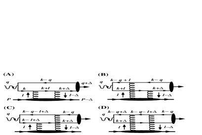
Figure 1: Four Feynman diagrams for $\gamma^{(*)}+N\rightarrow V(=J/\psi,\psi^{\prime})+N$ with momentum labeling.

The differential cross section with the small momentum transfer $t$ to the nucleon has the form

$$\frac{d\sigma(\gamma^{(*)}N\rightarrow VN)}{dt}$$

$$= \frac{1}{16\pi W^{4}}\sum_{pol.=L,T}\left|{\rm Im}{\cal M}^{pol.}(t)+i\,{\rm Re}{\cal M}^{pol.}(t)\right|^{2},$$

where the suffix ’$pol.$’ denotes the polarizations of the incoming photon. The imaginary part of the amplitude ${\cal M}^{pol.}$ is of the form

$${\rm Im}{\cal M}^{pol.}(t)$$ (5)

$$= \frac{\pi s}{\sqrt{2N_{c}}}\int_{0}^{1}d\alpha\int\frac{d\mbox{\boldmath$k$}_{\perp}}{16\pi^{3}}\int d\mbox{\boldmath$l$}_{\perp}\frac{\alpha_{s}(\mbox{\boldmath$l$}_{\perp}^{2})}{\mbox{\boldmath$l$}_{\perp}^{2}(\mbox{\boldmath$l$}_{\perp}-\mbox{\boldmath$\Delta$}_{\perp})^{2}}$$

$$\times \tilde{\Gamma}(x_{1},x_{2},\mbox{\boldmath$l$}_{\perp}^{2},t)\,I^{pol.(\gamma\rightarrow V)}(\alpha,\mbox{\boldmath$k$}_{\perp},\mbox{\boldmath$l$}_{\perp},\mbox{\boldmath$\Delta$}_{\perp})$$

with the number of color $N_{c}=3$ and $\alpha_{s}=g^{2}/(4\pi)$, where $I^{pol.(\gamma\rightarrow V)}$ represents the transition $\gamma^{(*)}\rightarrow V$ such as

$$I^{pol.(\gamma\rightarrow V)}(\alpha,\mbox{\boldmath$k$}_{\perp},\mbox{\boldmath$l$}_{\perp},\mbox{\boldmath$\Delta$}_{\perp})$$ (6)

$$= \sum_{\lambda\lambda^{\prime}}\left[\Psi^{(A)}_{\gamma}(\alpha,\mbox{\boldmath$k$}_{\perp})-\Psi^{(B)}_{\gamma}(\alpha,\mbox{\boldmath$k$}_{\perp},\mbox{\boldmath$l$}_{\perp})\right.$$

$$\left.-\Psi^{(C)}_{\gamma}(\alpha,\mbox{\boldmath$k$}_{\perp},\mbox{\boldmath$l$}_{\perp},\mbox{\boldmath$\Delta$}_{\perp})+\Psi^{(D)}_{\gamma}(\alpha,\mbox{\boldmath$k$}_{\perp},\mbox{\boldmath$\Delta$}_{\perp})\right]_{\lambda^{\prime}\lambda}$$

$$\times\ \Psi_{V\lambda\lambda^{\prime}}^{*}(\alpha,\mbox{\boldmath$k$}_{\perp},\mbox{\boldmath$\Delta$}_{\perp})$$

with the helicities of charm and anti-charm quarks, $\lambda^{\prime}$ and $\lambda$, respectively. The function $\tilde{\Gamma}(x_{1},x_{2},\mbox{\boldmath$l$}_{\perp}^{2},t)$ describing the lower part of Fig. 1, as mentioned in Sec. II A, has the form $\tilde{\Gamma}=f(x_{1},x_{2},\mbox{\boldmath$l$}_{\perp}^{2})\Gamma(t)$ with the two-gluon form factor,

$$\Gamma(t)=\frac{1}{\left(1-t/m_{2g}^{2}\right)^{2}},$$ (7)

where $m_{2g}$ denotes a mass scale relevant to this process FS . The skewed unintegrated gluon distribution $f(x_{1},x_{2},\mbox{\boldmath$l$}_{\perp}^{2})$ is related with

$$f(x_{1},x_{2},\mbox{\boldmath$l$}_{\perp}^{2})=\frac{\partial x_{2}G(x_{1},x_{2},\mbox{\boldmath$l$}_{\perp}^{2})}{\partial{\rm ln}\ \mbox{\boldmath$l$}_{\perp}^{2}},$$ (8)

using the skewed gluon distribution $G(x_{1},x_{2},\mbox{\boldmath$l$}_{\perp}^{2})$. The effect of skewedness can be then incorporated into a constant enhancement factor $R$ at small $x_{1}$ like the HERA experiment MR . Therefore, we rewrite the function $f(x_{1},x_{2},\mbox{\boldmath$l$}_{\perp}^{2})$ in terms of usual diagonal gluon distribution as

$$f(x_{1},x_{2},\mbox{\boldmath$l$}_{\perp}^{2})=\frac{R\ \partial x_{1}G(x_{1},\mbox{\boldmath$l$}_{\perp}^{2})}{\partial{\rm ln}\ \mbox{\boldmath$l$}_{\perp}^{2}}.$$ (9)

Here, $R=1.1\sim 1.2$ for the $J/\psi$ photoproduction MR and this factor gives an enhancement by $20\sim 40$ $\%$ for the cross section. Thus, we express the imaginary part of amplitude in terms of the diagonal gluon distribution, where hereafter we denote $x_{1}$ as $x$ for simplicity. Then, the real part in Eq. (LABEL:eqn:II-1) is related to the imaginary part as ${\rm Re}{\cal M}=-(\pi/2)(\partial\,{\rm Im}{\cal M})/(\partial\,{\rm ln}x)$ in the perturbative analysis BFGMS .

II.3 Light-cone wave function of photon

First, let us construct the LCWF of the incoming photon $\Psi_{\gamma}$ in Eq. (6), based on the LC perturbation theory LB ; BFGMS . It is defined as the following spinor matrix element

$$\Psi_{\gamma\lambda^{\prime}\lambda}^{pol.}(\alpha,\mbox{\boldmath$k$}_{\perp},\mbox{\boldmath$l$}_{\perp},\mbox{\boldmath$\Delta$}_{\perp})$$

$$= \frac{\overline{u}_{\lambda^{\prime}}(p_{i})}{\sqrt{\alpha}}\hbox to0.0pt{/\hss}{\mkern-1.0mu\varepsilon}_{\gamma}^{pol.}\frac{v_{\lambda}(q_{i})}{\sqrt{1-\alpha}}\frac{-ee_{c}\alpha(1-\alpha)}{\mbox{\boldmath$k$}_{\perp}^{(i)2}+m_{c}^{2}+\alpha(1-\alpha)Q^{2}},$$

where $\varepsilon_{\gamma}^{pol.}$ denotes $\varepsilon_{\gamma}^{0}=(q^{\prime}+xp^{\prime})/Q$ for the longitudinal polarization, and $\varepsilon_{\gamma}^{\perp}=(0,0,\mbox{\boldmath$\varepsilon$}_{\perp}^{\gamma})$ with $\mbox{\boldmath$\varepsilon$}_{\perp}^{\gamma}=\frac{1}{\sqrt{2}}(1,\gamma i)$ and $\gamma=\pm 1$ for the transverse polarization. Here, $\varepsilon_{\gamma}^{pol.}\cdot q=\varepsilon_{\gamma}^{0}\cdot\varepsilon_{\gamma}^{\perp}=0$. $e_{c}$ is the charge of charm quark $2/3$ in the units of $e$. $p_{i}$ and $q_{i}$ are the momenta of charm and anti-charm quarks with the helicities $\lambda^{\prime}$ and $\lambda$ respectively, for each diagram $(i)$ illustrated in Fig. 1. We define $\mbox{\boldmath$k$}_{\perp}^{(i)}$ as $\mbox{\boldmath$k$}_{\perp}^{(A)}=\mbox{\boldmath$k$}_{\perp}$, $\mbox{\boldmath$k$}_{\perp}^{(B)}=\mbox{\boldmath$k$}_{\perp}+\mbox{\boldmath$l$}_{\perp}$, $\mbox{\boldmath$k$}_{\perp}^{(C)}=\mbox{\boldmath$k$}_{\perp}-\mbox{\boldmath$l$}_{\perp}+\mbox{\boldmath$\Delta$}_{\perp}$ and $\mbox{\boldmath$k$}_{\perp}^{(D)}=\mbox{\boldmath$k$}_{\perp}+\mbox{\boldmath$\Delta$}_{\perp}$ for the corresponding diagram. After calculation of the spinor matrix elements, the results of the longitudinal polarization are given by

$$\Psi_{\gamma\lambda^{\prime}\lambda}^{long.} = 0$$ (11)

for $\lambda^{\prime}=\lambda$, and

$$\Psi_{\gamma\lambda^{\prime}\lambda}^{long.} = \frac{ee_{c}}{Q}\left[1-\frac{2\alpha(1-\alpha)Q^{2}}{\mbox{\boldmath$k$}_{\perp}^{(i)2}+m_{c}^{2}+\alpha(1-\alpha)Q^{2}}\right]$$ (12)

for $\lambda^{\prime}=-\lambda$. Here, the factor 1 in the first term of Eq.(12) disappears, when one takes a sum of four diagrams in calculation of the amplitude, and thus one neglects the factor. The results of the transverse polarization are

$$\Psi_{\gamma\lambda^{\prime}\lambda}^{trans.(\gamma)} = -\frac{\sqrt{2}ee_{c}\lambda\delta_{\gamma,\lambda}m_{c}}{\mbox{\boldmath$k$}_{\perp}^{(i)2}+m_{c}^{2}+\alpha(1-\alpha)Q^{2}}$$ (13)

for $\lambda^{\prime}=\lambda$, and

$$\Psi_{\gamma\lambda^{\prime}\lambda}^{trans.(\gamma)}=-\frac{2ee_{c}(\alpha-\delta_{\lambda,\gamma})\mbox{\boldmath$\varepsilon$}_{\perp}^{\gamma}\cdot\mbox{\boldmath$k$}_{\perp}^{(i)}}{\mbox{\boldmath$k$}_{\perp}^{(i)2}+m_{c}^{2}+\alpha(1-\alpha)Q^{2}}$$ (14)

for $\lambda^{\prime}=-\lambda$.

II.4 Light-cone wave function of charmonium

Next, we describe the LCWF of the outgoing charmonium produced through the soft hadronization process of the $c\bar{c}$ state, $\Psi_{V}$. It is defined in analogy with that of a photon. However, one should pay attention to new contribution from non-zero momentum of $\mbox{\boldmath$\Delta$}_{\perp}$, different from the case of the photon. Namely, the center of mass motion of the charmonium deviates by $\mbox{\boldmath$\Delta$}_{\perp}$ to a direction perpendicular to the incoming photon, due to a recoil of the target nucleon. Therefore, we introduce new null vectors $\bar{q^{\prime}}$ and $\bar{p^{\prime}}$ to redefine $(q+\Delta)^{+}$ as the longitudinal direction of $\Psi_{V}$. Here, $\bar{q^{\prime}}$ and $\bar{p^{\prime}}$ are expressed as $\bar{q^{\prime}}=q^{\prime}-(t/s)p^{\prime}+\Delta_{\perp}$ and $\bar{p^{\prime}}=-(t/s)q^{\prime}+p^{\prime}-\Delta_{\perp}$ up to $O(1/s)$ in terms of $q^{\prime}$ and $p^{\prime}$. The momenta of two quarks in the $c\bar{c}$ state, $k+\Delta$ and $k-q$, are written as

$$k+\Delta = \alpha\bar{q^{\prime}}+\left[\frac{\alpha t}{s}+\beta+\frac{Q^{2}-t+M_{\psi}^{2}}{s}\right]\bar{p^{\prime}}$$

$$+k_{\perp}+(1-\alpha)\Delta_{\perp},$$

$$k-q = (\alpha-1)\bar{q^{\prime}}+\left[\frac{\alpha t}{s}+\beta+\frac{Q^{2}-t}{s}\right]\bar{p^{\prime}}$$ (15)

$$+k_{\perp}+(1-\alpha)\Delta_{\perp}.$$

Using these relations, we find that the relative momentum between $c$ and $\bar{c}$ is $k_{\perp}+(1-\alpha)\Delta_{\perp}$. The polarization vectors of the charmonium are also rewritten in terms of $q^{\prime}$ and $p^{\prime}$ as $\varepsilon_{\psi}^{0}=[q^{\prime}-(M_{\psi}^{2}+t)p^{\prime}/s+\Delta_{\perp}]/M_{\psi}$ for the longitudinal polarization, and $\varepsilon_{\psi}^{\perp}=\varepsilon_{\gamma}^{\perp}+2(\Delta_{\perp}\cdot\varepsilon_{\gamma}^{\perp})(q^{\prime}-p^{\prime})/s$ for the transverse one. Here, $\varepsilon_{\psi}^{0}\cdot(q+\Delta)=\varepsilon_{\psi}^{\perp}\cdot(q+\Delta)=\varepsilon_{\psi}^{0}\cdot\varepsilon_{\psi}^{\perp}=0$. Using those polarization vectors, the LCWF of the charmonium $\Psi_{V}$ has the form

$$\Psi_{V\lambda\lambda^{\prime}}^{pol.*}(\alpha,\mbox{\boldmath$k$}_{\perp},\mbox{\boldmath$\Delta$}_{\perp}) = \frac{\overline{v}_{\lambda}(q-k)}{\sqrt{1-\alpha}}\hbox to0.0pt{/\hss}{\mkern-1.0mu\varepsilon}_{\psi}^{pol.*}{\cal R}\frac{u_{\lambda^{\prime}}(k+\Delta)}{\sqrt{\alpha}}$$ (16)

$$\times \frac{\phi_{\psi}^{*}(\alpha,\mbox{\boldmath$k$}_{\perp}+(1-\alpha)\mbox{\boldmath$\Delta$}_{\perp})}{M_{\psi}},$$

where ${\cal R}$ represents the projector introduced in HST2 ; HST3 , which keeps the $c\bar{c}$ state to be low-lying $1S$ state, given as ${\cal R}=\left[1+(\hbox to0.0pt{/\hss}{\mkern-1.0muq}+\hbox to0.0pt{/\hss}{\mkern-1.0mu\Delta})/M_{\psi}\right]/2$. Following HST3 , we further take into account the off-shellness of the spinor matrix element, $\overline{v_{\lambda}}\hbox to0.0pt{/\hss}{\mkern-1.0mu\varepsilon}_{\psi}^{pol.*}{\cal R}u_{\lambda^{\prime}}$, as the proper treatment. This spinor matrix element representing the effective “$c\bar{c}\rightarrow V$ vertex” may be off the energy shell and thus the total energy carried by the two spinors $\bar{v}_{\lambda}$ and $u_{\lambda^{\prime}}$ is generally different from the energy of the vector meson. This contribution should give $O(v^{2})$ corrections in the final result (In more detail, see HST3 ). For the longitudinal polarization, the results lead to

$$\Psi_{V\lambda\lambda^{\prime}}^{long.*} = -\sqrt{2}\lambda(1-2\alpha)\mbox{\boldmath$\varepsilon$}_{\perp}^{(\lambda)}\cdot(\mbox{\boldmath$k$}_{\perp}+(1-\alpha)\mbox{\boldmath$\Delta$}_{\perp})$$ (17)

$$\times \frac{\phi_{\psi}^{*}(\alpha,\mbox{\boldmath$k$}_{\perp}+(1-\alpha)\mbox{\boldmath$\Delta$}_{\perp})}{2\alpha(1-\alpha)M_{\psi}}$$

for $\lambda^{\prime}=\lambda$, and

$$\Psi_{V\lambda\lambda^{\prime}}^{long.*} = -\frac{1}{2}\left[1+\frac{(\mbox{\boldmath$k$}_{\perp}+(1-\alpha)\mbox{\boldmath$\Delta$}_{\perp})^{2}+m_{c}(M_{\psi}+m_{c})}{\alpha(1-\alpha)M_{\psi}^{2}}\right]$$ (18)

$$\times \phi_{\psi}^{*}(\alpha,\mbox{\boldmath$k$}_{\perp}+(1-\alpha)\mbox{\boldmath$\Delta$}_{\perp})$$

for $\lambda^{\prime}=-\lambda$, where $\mbox{\boldmath$\varepsilon$}_{\perp}^{(\lambda)}=\frac{1}{\sqrt{2}}(1,\lambda i)$. For the transverse polarization, similarly,

$$\Psi_{V\lambda\lambda^{\prime}}^{trans.(\gamma^{\prime})*} = \sqrt{2}\lambda\left[\delta_{\gamma^{\prime},\lambda}\left\{(M_{\psi}+m_{c})m_{c}+\alpha(1-\alpha)M_{\psi}^{2}\right\}\right.$$ (19)

$$\left.+2\delta_{\gamma^{\prime},-\lambda}\left\{\mbox{\boldmath$\varepsilon$}_{\perp}^{\gamma^{\prime}*}\cdot(\mbox{\boldmath$k$}_{\perp}+(1-\alpha)\mbox{\boldmath$\Delta$}_{\perp})\right\}^{2}\right]$$

$$\times \frac{\phi_{\psi}^{*}(\alpha,\mbox{\boldmath$k$}_{\perp}+(1-\alpha)\mbox{\boldmath$\Delta$}_{\perp})}{2\alpha(1-\alpha)M_{\psi}^{2}}$$

for $\lambda^{\prime}=\lambda$, and

$$\Psi_{V\lambda\lambda^{\prime}}^{trans.(\gamma^{\prime})*} = 2\mbox{\boldmath$\varepsilon$}_{\perp}^{\gamma^{\prime}*}\cdot(\mbox{\boldmath$k$}_{\perp}+(1-\alpha)\mbox{\boldmath$\Delta$}_{\perp})$$ (20)

$$\times \left[(\alpha-\delta_{\gamma,\lambda})(M_{\psi}+2m_{c})+(1-2\alpha)m_{c}\right]$$

$$\times \frac{\phi_{\psi}^{*}(\alpha,\mbox{\boldmath$k$}_{\perp}+(1-\alpha)\mbox{\boldmath$\Delta$}_{\perp})}{2\alpha(1-\alpha)M_{\psi}^{2}}$$

for $\lambda^{\prime}=-\lambda$. The suffix $\gamma^{\prime}$ denotes the polarization $\gamma^{\prime}=\pm 1$ in the transverse direction.

II.5 Detailed derivation of differential cross section

We focus on the process of $S$-channel helicity conservation (SCHC) between the initial photon and the final charmonium, because the HERA experiment demonstrates that, to good accuracy, the hypothesis of SCHC holds in the kinematical range $30<W<200$ GeV and $|t|<1$ GeV^-2 ZEUS02 . We obtain the following expressions for $I^{pol.(\gamma\rightarrow V)}$ of Eq. (6), using Eqs. (11)-(14) and (17)-(20): for the longitudinal channel of $\gamma(L)\rightarrow\psi(L)$,

$$I^{L\rightarrow L} = 2ee_{c}\alpha(1-\alpha)Q\ \Phi_{1}$$ (21)

$$\times \left[1+\frac{(\mbox{\boldmath$k$}_{\perp}+(1-\alpha)\mbox{\boldmath$\Delta$}_{\perp})^{2}+m_{c}(M_{\psi}+m_{c})}{\alpha(1-\alpha)M_{\psi}^{2}}\right]$$

$$\times \phi_{\psi}^{*}(\alpha,\mbox{\boldmath$k$}_{\perp}+(1-\alpha)\mbox{\boldmath$\Delta$}_{\perp})\ ;$$

for the transverse channel of $\gamma(T)\rightarrow\psi(T)$,

$$I^{T(\gamma)\rightarrow T(\gamma)} = -\frac{ee_{c}}{\alpha(1-\alpha)M_{\psi}^{2}}$$ (22)

$$\times \left[m_{c}\left\{(M_{\psi}+m_{c})m_{c}+\alpha(1-\alpha)M_{\psi}^{2}\right\}\Phi_{1}\right.$$

$$- 2\left.\left\{(2\alpha(1-\alpha)-1)M_{\psi}-m_{c}\right\}\mbox{\boldmath$\varepsilon$}_{\perp}^{\gamma}\cdot\vec{\Phi}_{2}\right.$$

$$\times\left.\mbox{\boldmath$\varepsilon$}_{\perp}^{\gamma*}\cdot(\mbox{\boldmath$k$}_{\perp}+(1-\alpha)\mbox{\boldmath$\Delta$}_{\perp})\right]$$

$$\times\phi_{\psi}^{*}(\alpha,\mbox{\boldmath$k$}_{\perp}+(1-\alpha)\mbox{\boldmath$\Delta$}_{\perp})\ .$$

Here, conveniently we defined the sum of energy denominator as

$$\Phi_{1} = \frac{1}{\mbox{\boldmath$k$}_{\perp}^{2}+\overline{Q}^{2}}-\frac{1}{(\mbox{\boldmath$k$}_{\perp}+\mbox{\boldmath$l$}_{\perp})^{2}+\overline{Q}^{2}}$$

$$- \frac{1}{(\mbox{\boldmath$k$}_{\perp}+\mbox{\boldmath$\Delta$}_{\perp}-\mbox{\boldmath$l$}_{\perp})^{2}+\overline{Q}^{2}}+\frac{1}{(\mbox{\boldmath$k$}_{\perp}+\mbox{\boldmath$\Delta$}_{\perp})^{2}+\overline{Q}^{2}}\ ,$$

$$\vec{\Phi}_{2} = \frac{\mbox{\boldmath$k$}_{\perp}}{\mbox{\boldmath$k$}_{\perp}^{2}+\overline{Q}^{2}}-\frac{\mbox{\boldmath$k$}_{\perp}+\mbox{\boldmath$l$}_{\perp}}{(\mbox{\boldmath$k$}_{\perp}+\mbox{\boldmath$l$}_{\perp})^{2}+\overline{Q}^{2}}$$

$$- \frac{\mbox{\boldmath$k$}_{\perp}+\mbox{\boldmath$\Delta$}_{\perp}-\mbox{\boldmath$l$}_{\perp}}{(\mbox{\boldmath$k$}_{\perp}+\mbox{\boldmath$\Delta$}_{\perp}-\mbox{\boldmath$l$}_{\perp})^{2}+\overline{Q}^{2}}+\frac{\mbox{\boldmath$k$}_{\perp}+\mbox{\boldmath$\Delta$}_{\perp}}{(\mbox{\boldmath$k$}_{\perp}+\mbox{\boldmath$\Delta$}_{\perp})^{2}+\overline{Q}^{2}}\ ,$$

where $\overline{Q}^{2}=m_{c}^{2}+\alpha(1-\alpha)Q^{2}$.

Now we are in a position to perform analytical integrations over $\mbox{\boldmath$l$}_{\perp}$ and $\mbox{\boldmath$k$}_{\perp}$ in the amplitude (5). First, we explain the integration over $\mbox{\boldmath$l$}_{\perp}$, assuming the range of $\mbox{\boldmath$l$}_{\perp}^{2}$ relevant in this process as $\mbox{\boldmath$\Delta$}_{\perp}^{2}\ll\mbox{\boldmath$l$}_{\perp}^{2}\ll\overline{Q}^{2}+\mbox{\boldmath$k$}_{\perp}^{2}$. This permits one to make an approximation $1/(\mbox{\boldmath$l$}_{\perp}-\mbox{\boldmath$\Delta$}_{\perp})^{2}\simeq 1/\mbox{\boldmath$l$}_{\perp}^{2}$ for the gluon propagators in Eq. (5). Then, the $\mbox{\boldmath$l$}_{\perp}$-integration for $\Phi_{1}$ in the integrand of Eq. (5) leads to

$$\int_{\mu^{2}}^{\overline{Q}^{2}+\mbox{\boldmath$k$}_{\perp}^{2}}d\mbox{\boldmath$l$}_{\perp}\frac{\alpha_{s}(\mbox{\boldmath$l$}_{\perp}^{2})}{\mbox{\boldmath$l$}_{\perp}^{2}}\frac{\partial xG(x,\mbox{\boldmath$l$}_{\perp})}{\partial\mbox{\boldmath$l$}_{\perp}^{2}}\Phi_{1}(\alpha,\mbox{\boldmath$k$}_{\perp},\mbox{\boldmath$l$}_{\perp},\mbox{\boldmath$\Delta$}_{\perp})$$

$$\simeq \pi\alpha_{s}(\overline{Q}^{2}+\mbox{\boldmath$k$}_{\perp}^{2})xG(x,\overline{Q}^{2}+\mbox{\boldmath$k$}_{\perp}^{2})\ F_{1}(\alpha,\mbox{\boldmath$k$}_{\perp},\mbox{\boldmath$\Delta$}_{\perp})$$

with

$$F_{1}(\alpha,\mbox{\boldmath$k$}_{\perp},\mbox{\boldmath$\Delta$}_{\perp})=-\frac{1}{\left(\mbox{\boldmath$k$}_{\perp}^{2}+\overline{Q}^{2}\right)^{2}}+\frac{2\overline{Q}^{2}}{\left(\mbox{\boldmath$k$}_{\perp}^{2}+\overline{Q}^{2}\right)^{3}}$$

$$- \frac{1}{\left\{(\mbox{\boldmath$k$}_{\perp}+\mbox{\boldmath$\Delta$}_{\perp})^{2}+\overline{Q}^{2}\right\}^{2}}+\frac{2\overline{Q}^{2}}{\left\{(\mbox{\boldmath$k$}_{\perp}+\mbox{\boldmath$\Delta$}_{\perp})^{2}+\overline{Q}^{2}\right\}^{3}}.$$

(26)

Here, we integrated from the low energy cut-off $\mu^{2}$($\sim\Lambda_{QCD}^{2}$) to $\overline{Q}^{2}+\mbox{\boldmath$k$}_{\perp}^{2}$ RRML ; MR over $\mbox{\boldmath$l$}_{\perp}^{2}$. Similarly, for $\mbox{\boldmath$\varepsilon$}_{\perp}^{\gamma}\cdot\vec{\Phi}_{2}$ in the integrand of Eq. (5), we get

$$\int_{\mu^{2}}^{\overline{Q}^{2}+\mbox{\boldmath$k$}_{\perp}^{2}}d\mbox{\boldmath$l$}_{\perp}\frac{\alpha_{s}(\mbox{\boldmath$l$}_{\perp}^{2})}{\mbox{\boldmath$l$}_{\perp}^{2}}\frac{\partial xG(x,\mbox{\boldmath$l$}_{\perp})}{\partial\mbox{\boldmath$l$}_{\perp}^{2}}\mbox{\boldmath$\varepsilon$}_{\perp}^{\gamma}\cdot\vec{\Phi}_{2}(\alpha,\mbox{\boldmath$k$}_{\perp},\mbox{\boldmath$l$}_{\perp},\mbox{\boldmath$\Delta$}_{\perp})$$

$$\simeq \pi\alpha_{s}(\overline{Q}^{2}+\mbox{\boldmath$k$}_{\perp}^{2})xG(x,\overline{Q}^{2}+\mbox{\boldmath$k$}_{\perp}^{2})\ \mbox{\boldmath$\varepsilon$}_{\perp}^{\gamma}\cdot\vec{F}_{2}(\alpha,\mbox{\boldmath$k$}_{\perp},\mbox{\boldmath$\Delta$}_{\perp})$$

with

$$\mbox{\boldmath$\varepsilon$}_{\perp}^{\gamma}\cdot\vec{F}_{2}(\alpha,\mbox{\boldmath$k$}_{\perp},\mbox{\boldmath$\Delta$}_{\perp})=$$

$$2\overline{Q}^{2}\left[\frac{\mbox{\boldmath$\varepsilon$}_{\perp}^{\gamma}\cdot\mbox{\boldmath$k$}_{\perp}}{\left(\mbox{\boldmath$k$}_{\perp}^{2}+\overline{Q}^{2}\right)^{3}}+\frac{\mbox{\boldmath$\varepsilon$}_{\perp}^{\gamma}\cdot(\mbox{\boldmath$k$}_{\perp}+\mbox{\boldmath$\Delta$}_{\perp})}{\left\{(\mbox{\boldmath$k$}_{\perp}+\mbox{\boldmath$\Delta$}_{\perp})^{2}+\overline{Q}^{2}\right\}^{3}}\right],$$

where we neglected $O\left((\mbox{\boldmath$l$}_{\perp}^{2}/\overline{Q}^{2})^{2}\right)$ terms in the LLA.

Next, we analytically perform the angular integration over $\mbox{\boldmath$k$}_{\perp}$ in Eq. (5). We introduce a new integral variable, $\mbox{\boldmath$K$}_{\perp}=\mbox{\boldmath$k$}_{\perp}+(1-\alpha)\mbox{\boldmath$\Delta$}_{\perp}$, instead of $\mbox{\boldmath$k$}_{\perp}$, to rewrite the nonperturbative wave function $\phi_{\psi}(\alpha,\mbox{\boldmath$k$}_{\perp}+(1-\alpha)\mbox{\boldmath$\Delta$}_{\perp})$ as a function of one variable, $\mbox{\boldmath$K$}_{\perp}$. Here, we stress that, as mentioned in Sec. I, the contribution of $\mbox{\boldmath$\Delta$}_{\perp}$ is not suppressed compared with that of $\mbox{\boldmath$k$}_{\perp}$ in the argument of wave function, and thus we should exactly include the kinematical corrections of $\mbox{\boldmath$\Delta$}_{\perp}$ by such a redefinition of the argument. When we define the angle $\theta$ as $\mbox{\boldmath$K$}_{\perp}\cdot\mbox{\boldmath$\Delta$}_{\perp}=|\mbox{\boldmath$K$}_{\perp}||\mbox{\boldmath$\Delta$}_{\perp}|\,{\rm cos}\,\theta$, the $\theta$-integrations of $F_{1}$ and $\vec{F}_{2}$ yield the following results:

$$\int_{0}^{2\pi}d\theta F_{1}(\alpha,\mbox{\boldmath$K$}_{\perp},\mbox{\boldmath$\Delta$}_{\perp})$$ (29)

$$= -\frac{4\pi}{\left(\mbox{\boldmath$K$}_{\perp}^{2}+\overline{Q}^{2}\right)^{2}}$$

$$\times\left[1+\frac{2\{(\alpha^{2}+(1-\alpha)^{2})\mbox{\boldmath$\Delta$}_{\perp}^{2}-\overline{Q}^{2}\}}{\mbox{\boldmath$K$}_{\perp}^{2}+\overline{Q}^{2}}\right.$$

$$-\frac{12(\alpha^{2}+(1-\alpha)^{2})\mbox{\boldmath$\Delta$}_{\perp}^{2}\overline{Q}^{2}}{\left(\mbox{\boldmath$K$}_{\perp}^{2}+\overline{Q}^{2}\right)^{2}}$$

$$+\left.\frac{12(\alpha^{2}+(1-\alpha)^{2})\mbox{\boldmath$\Delta$}_{\perp}^{2}\overline{Q}^{4}}{\left(\mbox{\boldmath$K$}_{\perp}^{2}+\overline{Q}^{2}\right)^{3}}\right],$$

$$\int_{0}^{2\pi}d\theta\ \mbox{\boldmath$\varepsilon$}_{\perp}^{\gamma}\cdot\vec{F}_{2}(\alpha,\mbox{\boldmath$K$}_{\perp},\mbox{\boldmath$\Delta$}_{\perp})\ \mbox{\boldmath$\varepsilon$}_{\perp}^{\gamma*}\cdot\mbox{\boldmath$K$}_{\perp}$$ (30)

$$= \frac{4\pi\mbox{\boldmath$K$}_{\perp}^{2}\overline{Q}^{2}}{\left(\mbox{\boldmath$K$}_{\perp}^{2}+\overline{Q}^{2}\right)^{3}}\left[1+\frac{3(\alpha^{2}+(1-\alpha)^{2})\mbox{\boldmath$\Delta$}_{\perp}^{2}}{\mbox{\boldmath$K$}_{\perp}^{2}+\overline{Q}^{2}}\right.$$

$$-\left.\frac{6(\alpha^{2}+(1-\alpha)^{2})\mbox{\boldmath$\Delta$}_{\perp}^{2}\overline{Q}^{2}}{\left(\mbox{\boldmath$K$}_{\perp}^{2}+\overline{Q}^{2}\right)^{2}}\right].$$

Here, we left the $t$-dependent terms up to $O\left(\mbox{\boldmath$\Delta$}_{\perp}^{2}/(\mbox{\boldmath$K$}_{\perp}^{2}+\overline{Q}^{2})\right)$. Therefore, in the photoproduction, this implies that the applicable range of $t$ should be $|t|\ll m_{c}^{2}$ and we should discuss numerical results in the small regions of $|t|<1$ GeV² in Sec. III.

Finally, using Eqs. (29) and (30), we arrive at the whole expressions for the imaginary part of amplitude (6): for $\gamma(L)\rightarrow\psi(L)$,

$${\rm Im}\ {\cal M}^{L}(t)=-\frac{2\sqrt{2}\pi^{2}ee_{c}QsR}{\sqrt{N_{c}}}\int_{0}^{1}d\alpha\alpha(1-\alpha)$$

$$\times \alpha_{s}(\overline{Q}^{2}+\mbox{\boldmath$k$}_{\perp}^{2})xG(x,\overline{Q}^{2}+\mbox{\boldmath$k$}_{\perp}^{2})$$

$$\times \int_{0}^{\infty}\frac{d\mbox{\boldmath$K$}_{\perp}^{2}}{16\pi^{2}}\frac{\phi_{\psi}^{*}(\alpha,\mbox{\boldmath$K$}_{\perp})}{\left(\mbox{\boldmath$K$}_{\perp}^{2}+\overline{Q}^{2}\right)^{2}}$$

$$\times\left(1+\frac{\mbox{\boldmath$K$}_{\perp}^{2}+m_{c}(M_{\psi}+m_{c})}{\alpha(1-\alpha)M_{\psi}^{2}}\right)$$

$$\times \left[H_{1}(\alpha,\mbox{\boldmath$K$}_{\perp})+\frac{2(\alpha^{2}+(1-\alpha)^{2})(-t)}{\mbox{\boldmath$K$}_{\perp}^{2}+\overline{Q}^{2}}H_{2}(\alpha,\mbox{\boldmath$K$}_{\perp})\right]\ ;$$

for $\gamma(T)\rightarrow\psi(T)$,

$${\rm Im}\ {\cal M}^{T}(t)=-\frac{\sqrt{2}\pi^{2}ee_{c}sR}{\sqrt{N_{c}}M_{\psi}^{2}}\int_{0}^{1}\frac{d\alpha}{\alpha(1-\alpha)}$$ (32)

$$\times \alpha_{s}(\overline{Q}^{2}+\mbox{\boldmath$k$}_{\perp}^{2})xG(x,\overline{Q}^{2}+\mbox{\boldmath$k$}_{\perp}^{2})$$

$$\times\int_{0}^{\infty}\frac{d\mbox{\boldmath$K$}_{\perp}^{2}}{16\pi^{2}}\frac{\phi_{\psi}^{*}(\alpha,\mbox{\boldmath$K$}_{\perp})}{\left(\mbox{\boldmath$K$}_{\perp}^{2}+\overline{Q}^{2}\right)^{2}}$$

$$\times \Biggl{[}-m_{c}\left\{(M_{\psi}+m_{c})m_{c}+\alpha(1-\alpha)M_{\psi}^{2}\right\}H_{1}(\alpha,\mbox{\boldmath$K$}_{\perp})\Biggr{.}$$

$$+\ 2\left\{(\alpha^{2}+(1-\alpha)^{2})M_{\psi}+m_{c}\right\}\frac{\mbox{\boldmath$K$}_{\perp}^{2}\overline{Q}^{2}}{\mbox{\boldmath$K$}_{\perp}^{2}+\overline{Q}^{2}}$$

$$+ \frac{2(\alpha^{2}+(1-\alpha)^{2})(-t)}{\mbox{\boldmath$K$}_{\perp}^{2}+\overline{Q}^{2}}$$

$$\times\Biggl{\{}-m_{c}\left((M_{\psi}+m_{c})m_{c}+\alpha(1-\alpha)M_{\psi}^{2}\right)H_{2}(\alpha,\mbox{\boldmath$K$}_{\perp})\Biggr{.}$$

$$\qquad+3\left((\alpha^{2}+(1-\alpha)^{2})M_{\psi}+m_{c}\right)$$

$$\qquad\times\left.\left.\frac{\mbox{\boldmath$K$}_{\perp}^{2}\overline{Q}^{2}}{\mbox{\boldmath$K$}_{\perp}^{2}+\overline{Q}^{2}}H_{1}(\alpha,\mbox{\boldmath$K$}_{\perp})\right\}\right].$$

Here, we define

$$H_{1}(\alpha,\mbox{\boldmath$K$}_{\perp}) = 1-\frac{2\overline{Q}^{2}}{\mbox{\boldmath$K$}_{\perp}^{2}+\overline{Q}^{2}},$$

$$H_{2}(\alpha,\mbox{\boldmath$K$}_{\perp}) = 1-\frac{6\overline{Q}^{2}}{\mbox{\boldmath$K$}_{\perp}^{2}+\overline{Q}^{2}}+\frac{6\overline{Q}^{4}}{\left(\mbox{\boldmath$K$}_{\perp}^{2}+\overline{Q}^{2}\right)^{2}}.$$ (33)

To determine the nonperturbative part of the charmonium wave functions, $\phi_{\psi}(\alpha,\mbox{\boldmath$K$}_{\perp})$, we use the wave functions obtained by solving Schrödinger equation with the realistic potential FKS ; SHIAH . We adopt the Cornell potential model with the corresponding quark masses $m_{c}=1.5$ GeV QR , giving a good description of the charmonium wave functions. Here, we rewrite the non-relativistic wave function, $\phi_{\psi}^{NR}$, originally obtained in terms of three momenta, as a function of the LC variables, $\phi_{\psi}(\alpha,\mbox{\boldmath$K$}_{\perp})$, by simple kinematical replacement FKS ; SHIAH . For the diagonal gluon distribution $G$ in Eqs. (LABEL:eqn:II-26), (32), we employ Glück-Reya-Vogt parametrization for the next-to-leading order fits GRV95 .

Using Eqs. (LABEL:eqn:II-26) and (32), let us construct $B^{dip}_{V}(t)$ in Eq. (2), which comes from the upper part describing the transition $\gamma^{(*)}\rightarrow V$ in Fig.  1. One should note that, in our approximation up to the first order of $t$, $B^{dip}(t)$ is a function of $Q^{2}$ and $W$, whereas independent of $t$. Conventionally, we denote the imaginary part of the amplitudes as ${\rm Im}{\cal M}_{L(T)}={\cal A}^{Im}_{L(T)}+(-t)\tilde{\cal A}^{Im}_{L(T)}$, where ${\cal A}^{Im}_{L(T)}$ corresponds to the amplitude independent of $t$ in Eqs. (LABEL:eqn:II-26) and (32), and then $\tilde{\cal A}^{Im}_{L(T)}$ denotes the amplitude proportional to $t$. Similarly, for the real part, ${\rm Re}{\cal M}_{L(T)}={\cal A}^{Re}_{L(T)}+(-t)\tilde{\cal A}^{Re}_{L(T)}$. Using these amplitudes to the first order of $t$, $B^{dip}_{V}(W,Q^{2})$ is given by

$$B^{dip}_{V}(W,Q^{2})=-2\frac{\sum_{i=L,T}\left[{\cal A}^{Im}_{i}\tilde{\cal A}^{Im}_{i}+{\cal A}^{Re}_{i}\tilde{\cal A}^{Re}_{i}\right]}{\sum_{i=L,T}\left[\left({\cal A}^{Im}_{i}\right)^{2}+\left({\cal A}^{Re}_{i}\right)^{2}\right]}.$$ (34)

III Numerical results and comparison with data

In Fig. 2, we show the results of the dipole contribution (34) to the slope parameters, $B^{dip}_{V}$, as a function of $Q^{2}$. Those results are plotted as dashed line for $B^{dip}_{J/\psi}$, dash-dotted line for $B^{dip}_{\psi^{\prime}}$, and solid line for their difference $B^{dip}_{J/\psi}-B^{dip}_{\psi^{\prime}}$, at the fixed energy $W=85$ GeV.

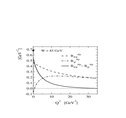
Figure 2: The slope parameters $B^{dip}_{J/\psi}$, $B^{dip}_{\psi^{\prime}}$, and $B^{dip}_{J/\psi}-B^{dip}_{\psi^{\prime}}$, plotted as a function of $Q^{2}$ at the fixed energy $W=85$ GeV. A blob at $Q^{2}=0$ represents $B_{J/\psi}-B_{\psi^{\prime}}$ from the data H102 for a reference.

$B^{dip}_{J/\psi}$ has the maximum value of $B^{dip}_{J/\psi}\simeq 0.48$ GeV^-2 and decreases with increasing $Q^{2}$, while $B^{dip}_{\psi^{\prime}}$ has the negative value near $Q^{2}=0$, $B^{dip}_{J/\psi}\simeq-0.07$ GeV^-2, and rapidly increases with increasing $Q^{2}$, taking the positive value. This feature changing the sign of the $t$-slope with $Q^{2}$ appears only in the $\psi^{\prime}$ production. This is an indication of the node inherent in the radial direction of the $2S$ wave function. At large $Q^{2}$, however, they approach each other, and then their difference reaches almost zero, because the size of the $c\bar{c}$-dipole state is squeezed with increasing $Q^{2}$ and the amplitudes are evaluated near the origin of the charmonium wave functions. We find the maximum value of the difference at $Q^{2}=0$, which is $B^{dip}_{J/\psi}-B^{dip}_{\psi^{\prime}}\simeq 0.53$ GeV^-2. Using Eq. (3), we can directly compare the result with the experimental data. In fact, it turns out that our result is consistent with H1 data H102 , which is $B_{J/\psi}-B_{\psi^{\prime}}\simeq 0.68$ GeV^-2 showed as a blob in Fig. 2, in the sign and the magnitude.

Similar behavior of the $t$-slope difference as a function of $Q^{2}$ was also confirmed in the analysis of NNPZZ for the transverse polarization. Their results show that the difference is about 0.25 GeV^-2 at $Q^{2}=0$ and $W=100$ GeV, which is about 2 times smaller than our result, and falls down more slowly with increasing $Q^{2}$.

In Fig. 3, we plot the slope parameters $B^{dip}_{J/\psi}$, $B^{dip}_{\psi^{\prime}}$, and $B^{dip}_{J/\psi}-B^{dip}_{\psi^{\prime}}$, as a function of $W$ at $Q^{2}=0$, similar to Fig. 2.

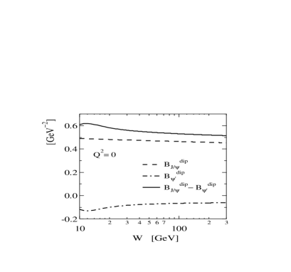
Figure 3: The $W$-dependence of the slope parameters $B^{dip}_{J/\psi}$, $B^{dip}_{\psi^{\prime}}$, and $B^{dip}_{J/\psi}-B^{dip}_{\psi^{\prime}}$, for photoproductions, compared with ZEUS data ZEUS02 .

Apparently, both $B^{dip}_{J/\psi}$ and $B^{dip}_{\psi^{\prime}}$ show an almost flat behavior as a function of $W$ and their absolute values even decrease slightly with increasing $W$. As a result, their difference $B^{dip}_{J/\psi}-B^{dip}_{\psi^{\prime}}$ is also almost independent of $W$. Such insensitive behaviors to $W$ are found also at moderate $Q^{2}$. On the other hand, the $t$-slope difference in NNPZZ shows stronger $W$-dependence as $W$ increasing: their result decreases by a factor $\sim 2$ from the moderate fixed-target energies to the HERA collider energies.

We can now compare the result of $B^{dip}_{J/\psi}$ with ZEUS data ZEUS02 by combining with the $t$-slope arising from the two-gluon form factor as in Eq. (2). Here, we simply set $t=0$ for the first term of (2), and then it adds a constant factor of $B_{N}$ to $B^{dip}_{J/\psi}$ as $B_{J/\psi}(t=0)=4.0+B^{dip}_{J/\psi}$. Using this relation, we find that the contribution of the $c\bar{c}$ state to the $t$-slope is not negligible, because the size can reach about 10 $\%$ of the whole at $Q^{2}=0$ for the $J/\psi$ production. Similarly for the $\psi^{\prime}$ production, it turns out that the contribution of the $c\bar{c}$ state becomes largest (about 5 $\%$) in the vicinity of $Q^{2}\sim 10$ GeV². The result of $B_{J/\psi}(W)$ is shown in Fig. 4 with the data measured for the muon and electron decay channels of $J/\psi$ separately.

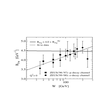
Figure 4: The $W$-dependence of the $t$-slope $B_{J/\psi}$ for the elastic $J/\psi$ photoproduction. The data was measured in two leptonic decay channels, $J/\psi\rightarrow\mu^{+}\mu^{-},e^{+}e^{-}$ ZEUS02 . The solid line shows our result $B_{J/\psi}(t=0)=4+B^{dip}_{J/\psi}$ in Eq. (2). The dotted line represents the fit to the data: $B_{V}(W)=B_{0}+4\alpha^{\prime}_{\bf P}\cdot{\rm ln}\,(W/90\,{\rm GeV})$ with $B_{0}=4.15$ GeV^-2 and $\alpha^{\prime}_{\bf P}=0.116$ GeV^-2 ZEUS02 .

The data indicate the increase of the $t$-slope with $W$ and this energy-dependent $t$-slope fits well to the data as a form of $B_{V}(W)=B_{0}+4\alpha^{\prime}_{\bf P}\cdot{\rm ln}\,(W/90\,{\rm GeV})$ with $B_{0}=4.15$ GeV^-2 and $\alpha^{\prime}_{\bf P}=0.116$ GeV^-2 ZEUS02 . Our $t$-slope almost independent of $W$ is in agreement with the data only in the range of $W=100\sim 200$ GeV. The reason for this behavior (solid line) is easily explained in our formulation: $B^{dip}_{V}(W)$ giving only the $W$-dependence in Eq. (2) has the form $B^{dip}_{V}\propto{\cal A}\tilde{\cal A}/{\cal A}^{2}$ in a simplest description, where ${\cal A}$($\tilde{\cal A}$) denotes the imaginary or real parts of the amplitude with either longitudinal or transverse polarizations. Then, the amplitudes has a common factor $xG(x)$ in the integrands. Usually, at HERA energies, the low-$x$ behavior of the gluon distribution $xG(x)$ is expected to be $xG(x)\sim x^{-\lambda}$ with $\lambda\simeq 0.2$, which is obtained from the analysis of the inclusive deep-inelastic scattering data. Here, $x\sim M_{\psi}^{2}/W^{2}$ at $Q^{2}=0$ and the $Q^{2}$-scale of $G$ is set to $Q^{2}\simeq m_{c}^{2}$. Following this simple parametrization for $xG(x)$, $B^{dip}_{V}$ is completely independent of $W$. In fact, $x$ and the scale $\overline{Q}^{2}+\mbox{\boldmath$k$}_{\perp}^{2}$ have $\alpha$, $\mbox{\boldmath$k$}_{\perp}$-dependences in our formulation. The corrections, however, give only a weak dependence of $B^{dip}_{V}$ on the energy $W$, illustrated in Fig. 4.

Thus, the energy-dependence of the $t$-slope, so called ”shrinkage”, observed by the ZEUS experiment, seems to need more sophisticated treatments for the $W$ dependence. For example, we may consider two possibilities as the origin of the $W$-dependence, which we have not taken into account here: one possible effect is the Gribov diffusion, which is known as a rapid expansion in the transverse size of the $c\bar{c}$-dipole state, created from a photon fluctuation as $W$ increases. This phenomenon leads to the shrinkage of a diffraction peak, which can be interpreted as an increase of the interaction radius BFGMS ; another effect is the increase of the $c\bar{c}$-dipole scattering off the peripheral pion-cloud of a nucleon with increasing $W$. As suggested in FS , at relatively low $W$($\sim 10$ GeV) such as the fixed-target energies, the contribution of the pions to the gluon distribution is not important. It is because the pions carry a smaller fraction of the nucleon momentum, so that the gluons inside the pions have much smaller momentum fraction than $x\sim 0.1$, which is the typical value of the momentum fraction at the energies. In this case, the authors of FS predict that the corresponding two-gluon form factor (7) is close to the axial form factor of the nucleon with $m_{2g}^{2}\simeq 1$ GeV². At higher collider energies of HERA (typically, $W\sim 100$ GeV), where it reaches $x\ll 0.01$, one should take into account the contribution from the pion-cloud. At high $W$, therefore, the form factor is expected to approach the electromagnetic one with $m_{2g}^{2}\simeq 0.71$ GeV² FS .

In order to check how the mass scale changes with $W$ in our approach, we try to reproduce the HERA data of the elastic $J/\psi$ photoproduction by changing a value of the mass scale. We neglect a contribution from the Gribov diffusion, because the pQCD analysis is inapplicable for a large size configuration due to the diffusion.

Resulting $t$-dependence of the $J/\psi$ cross section is shown in Fig. 5. It is compared with ZEUS data ZEUS02 for three representative ranges of $W$, i.e., $30<W<50$ GeV, $70<W<90$ GeV and $150<W<170$ GeV for the $\mu^{+}\mu^{-}$ decay of $J/\psi$, and $20<W<50$ GeV, $70<W<90$ GeV and $125<W<170$ GeV for the $e^{+}e^{-}$ decay. They are calculated over the kinematic range $|t|<0.8$ GeV^-2, in which our formulation could be applicable.

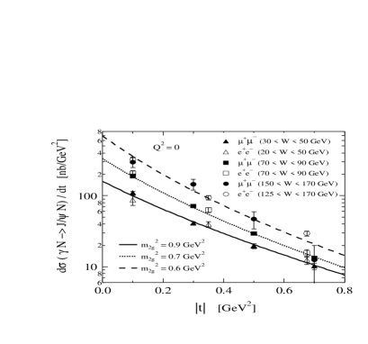
Figure 5: The differential cross section of elastic $J/\psi$ photoproduction, $\gamma+N\rightarrow J/\psi+N$, as a function of $|t|$, compared with ZEUS data ZEUS02 measured in two leptonic decay channels, $J/\psi\rightarrow\mu^{+}\mu^{-},e^{+}e^{-}$. The data are plotted for three representative ranges of $W$ for respective decay channels, as written in the figure. The solid, dotted and dashed curve show our results calculated in three corresponding $W$ ranges, $30<W<50$ GeV, $70<W<90$ GeV and $150<W<170$ GeV. Then good fits to the data require that the squared mass scale has the values 0.9, 0.7, 0.6 GeV² in respective $W$ regions.

Here, we set a parameter $R=1.2$ for the skewedness effect of the off-diagonal gluon distribution, which changes only the normalization of the cross section and thus does not affect the dependence of cross section on $t$. Further, to increase the overall magnitude of the cross section, we carry out a rescaling of $Q^{2}$ in the gluon distribution and the strong coupling constant rescale , following the work of FKS . It is also stressed that our naive treatment for the rescaling is almost insensitive to the $t$-slope, but it enhances only the normalization of the cross section about $30\sim 40$ $\%$.

The solid, dotted, and dashed curves represent our calculations corresponding to each $W$ range, $30<W<50$ GeV, $70<W<90$ GeV and $150<W<170$ GeV. They show an exponential decrease very close to the data with increasing $|t|$, when we take $m_{2g}^{2}=0.9,0.7,0.6$ GeV² in respective $W$ bins. Hence, to obtain a good agreement with the data, we find that the mass scale should decrease with increasing $W$ at HERA energies. This is qualitatively consistent with the suggestion of FS mentioned above.

IV Summary and discussion

To summarize, in the LLA of pQCD we have formulated $t$-dependences of the differential cross section for the diffractive (”elastic”) charmonia ($J/\psi$ and $\psi^{\prime}$) photo- and electroproductions at low $|t|$($<1$ GeV^-2). To deal with the production of the radially excited $2S$ state ($\psi^{\prime}$) together with that of $J/\psi$, we have employed the charmonium LCWF, properly including the sub-leading effects due to Fermi motion, based on a technique developed in HST2 ; HST3 . Following QCD factorization, the two-gluon form factor of the nucleon is assumed to be process-independent and we define it as a function of only $t$ scaled by the relevant squared mass in a dipole form. By assuming an exponential form of the differential cross section, following the standard experimental fit so far, we have calculated the diffractive $t$-slope, $B_{V}(t)$, over the $|t|$ range of less than 1 GeV².

The dipole part, $B^{dip}_{V}$, shows that the $Q^{2}$ dependence presents a distinct difference between $J/\psi$ and $\psi^{\prime}$, reflecting the properties of wave functions, i.e., a node effect for the $2S$ state. The former monotonically decreases with $Q^{2}$, while the latter has a negative value at small $Q^{2}$ and rapidly increases with $Q^{2}$, keeping $B^{dip}_{J/\psi}>B^{dip}_{\psi^{\prime}}$ in the realistic $Q^{2}$ region of HERA. Then, the difference $B_{J/\psi}-B_{\psi^{\prime}}$ shows a strong $Q^{2}$ dependence that tends to almost zero with increasing $Q^{2}$ associated with squeezing of the dipole, after achieving a maximum of $0.53$ GeV^-2 at $Q^{2}=0$ and $W=85$ GeV. This value at $Q^{2}=0$ is consistent with HERA data. It is noted that, to a good approximation, the difference should be free from a contribution of the Gribov diffusion, because such a contribution should be incorporated into the initial photon part in QCD factorization and it is expected to contribute at the same level for $J/\psi$ and $\psi^{\prime}$.

The $W$-dependences of $B^{dip}_{V}$ indicate almost a flat behavior at $Q^{2}=0$ (or also moderate $Q^{2}$), contrary to a shrinkage of $t$-slope observed at ZEUS. At small $x$, mainly two effects are expected to be the origin for such $W$-dependences of the $t$-slope: one comes from the dipole part, $\it i.e.$, the Gribov diffusion; another is due to the target nucleon, $\it i.e.$, the effect of hard probe scattering off the peripheral pion-cloud of a nucleon. We incorporated the latter phenomenon through the change of the mass scale appearing in the nucleon form factor, by fitting to ZEUS data for differential cross section of $J/\psi$ photoproductions at several $W$ ranges, although we neglected the former phenomenon for simplicity. To get a good fit to the data, we find significant decrease of the mass scale with increasing $W$, e.g., $0.6<m_{2g}^{2}<0.9$ GeV² in the region of $20<W<170$ GeV. This mass scale decreasing with $W$ will provide us with information concerning gluon distributions of the nucleon through a probe of $c\bar{c}$-dipole. Further detailed study on it might be useful for investigating not only the gluon distribution of the pion-cloud on the surface of nucleon, but also the non-linear property of gluons inside the nucleon, which will become more important with higher $W$.

On the other hand, the difference of $t$-slopes shows a behavior almost independent of $W$. This quantity is most likely free from the Gribov diffusion, as mentioned above. Unfortunately, the $W$-dependence of $B_{\psi^{\prime}}$ has been not yet observed so far. However, its observation has some importance and we would request early realization of such an observation. If the experiments observe somewhat the $W$ dependence for the difference of $t$-slopes, contrary to our prediction, then we might guess the following two origins:

1. The Gribov diffusion might introduce a large size effect upon the $c\bar{c}$-dipole at high $W$, thereby influencing the final hadronization dependence. It will give important information about the mechanism of the diffusion.

2. Otherwise, we could doubt the hypothesis for a universal form of nucleon form factor based on the factorization, which is very challenging.

Finally, we stress that the finite size effect of the $c\bar{c}$-dipole is not negligible for the $t$-slope of charmonia electroproductions at the HERA energies and $Q^{2}<30$ GeV². Combining both data from $J/\psi$ and $\psi^{\prime}$ productions, we can investigate the pure contribution of the dipole part in detail. Such a precise study will finally make it important to extract the detailed information of the gluon distribution in the nucleon by making use of the diffractive charmonium photoproductions. Recently, a fascinating study on the energy-dependent $t$-slope was reported in KT , using the dipole saturation model with an impact parameter dependence. A part of the $W$ dependence could also arise from the non-linear dynamics of the saturation for the gluon distribution in the target nucleon. The analysis including such an effect we consider to be interesting and is planned for one of our future works.

- (1) A. Hayashigaki, K. Suzuki and K. Tanaka, Nucl. Phys. A721(2003) 813c.
- (2) A. Hayashigaki, K. Suzuki and K. Tanaka, in preparation. In this work we formulate a certain Fermi motion effect up to corrections in a proper manner, based on idea developed in HST2 .
- (3) S.J. Brodsky, L. Frankfurt, J.F. Gunion, A.H. Mueller and M. Strikman, Phys. Rev. D50(1994) 3134.
- (4) H1 Collaboration, C. Adloff et al., Phys. Lett. B483(2000) 23.
- (5) ZEUS Collaboration, S. Chekanov et al., Eur. Phys. J. C24(2002) 345.
- (6) H1 Collaboration, C. Adloff et al., Phys. Lett. B541(2002) 251.
- (7) L. Frankfurt, W. Koepf and M. Strikman, Phys. Rev. D54(1996) 3194; ibid. D57(1998) 512.
- (8) M.G. Ryskin, R.G. Roberts, A.D. Martin and E.M. Levin, Z. Phys. C76(1997) 231.
- (9) G.P. Lepage and S.J. Brodsky, Phys. Rev. D22(1980) 2157.
- (10) J. Nemchik, N.N. Nikolaev, E. Predazzi, B.G. Zakharov and V.R. Zoller, JETP 86(6)(1998) 1054.
- (11) P. Hoyer and S. Peign, Phys. Rev. D61(2000) 031501(R).
- (12) K. Suzuki, A. Hayashigaki, K. Itakura, J. Alam and T. Hatsuda, Phys. Rev. D62(2000) 031501(R).
- (13) A.D. Martin, M.G. Ryskin and T. Teubner, Phys. Rev. D62(2000) 014022.
- (14) M.G. Ryskin, Y.M. Shabelski and A.G. Shuvaev, Phys. Lett. B446(1999) 48.
- (15) L. Frankfurt and M. Strikman, Phys. Rev. D66(2002) 031502(R).
- (16) A.D. Martin and M.G. Ryskin, Phys. Rev. D57(1998) 6692.
- (17) C. Quigg and J.L. Rosner, Phys. Lett. 71B(1977) 153 ; E. Eichten et al., Phys. Rev. Lett. D17(1978) 3090.
- (18) M. Glück, E. Reya and A. Vogt, Z. Phys. C67(1995) 433.
- (19) In numerical calculation, this rescaling is simply done by adopting , which is different from relations used in FKS , but it gives results close to FKS quantitatively HST3 .
- (20) H. Kowalski and D. Teaney, hep-ph/0304189.