Abstract

We present a detailed comparison of a variety of predictions for diffractive light vector meson production with the data collected at the HERA collider. All our calculations are performed within a dipole model framework and make use of different models for the meson light-cone wavefunction. There are no free parameters in any of the scenarios we consider. Generally we find good agreement with the data using rather simple Gaussian motivated wavefunctions in conjunction with dipole cross-sections which have been fitted to other data.

PACS Numbers: 12.40.Nn, 13.60.Le

1 Introduction

In a previous paper, Forshaw, Kerley and Shaw (FKS) [1] reported on a successful attempt to extract the cross-section for scattering colour dipoles of fixed transverse size off protons using both electroproduction and photoproduction $\gamma p$ total cross-section data, together with the constraint provided by the measured ratio of the diffraction dissociation cross-section to the total cross-section for real photons. Subsequently, the same model has been applied to “diffractive deep inelastic scatterring” (DDIS) $\gamma^{*}p\rightarrow X\,p$ [2] and also to deeply virtual Compton scattering (DVCS) $\gamma^{*}p\rightarrow\gamma\,p$ [3]. In both cases, the model was shown to yield predictions in agreement with the data [4, 5] with no adjustable parameters. The model can also be extended to diffractive vector meson production:

$$\gamma^{*}(q)+p(p)\rightarrow V(q^{\prime})+p(p^{\prime})\hskip 28.45274ptV=\rho,\phi~{}\mbox{or}~{}J/\Psi\;,$$ (1)

where the squared centre of mass energy $s=W^{2}=(p+q)^{2}\gg Q^{2},M_{V}^{2}$. In these processes the choice of vector meson, as well as of different photon virtualities, allows one to explore contributions from dipoles of different transverse sizes. The process also has the advantage that there is a wide range of available data. It ought also to provide important information on the poorly known light-cone wavefunctions of the the vector mesons.

The aim of this paper is to confront the predictions of the dipole model with the HERA data on $\rho$ and $\phi$ electroproduction. The predictions for $J/\Psi$ production are best considered in conjunction with an analysis of open charm production, and will be discussed elsewhere. We shall focus on the FKS model [1], but we also compare with the predictions of two other models: the Golec-Biernat-Wüsthoff (GW) saturation model [6, 7]; and the recent “Colour Glass Condensate” (CGC) model of Iancu, Itakura and Munier [8]. For the meson light-cone wavefunction, we shall consider three different ansätze: the Dosch, Gousset, Kulzinger and Pirner (DGKP) [9] model; the Nemchik, Nikolaev, Predazzi and Zakharov (NNPZ) [10] model; and a simple “boosted Gaussian” wavefunction, which can be considered as a special case of the latter.

The paper is laid out as follows. In the first two sections we summarise the dipole models used and discuss the forms chosen for the vector meson wavefunctions. We then compare their predictions with experiment before drawing our conclusions.

2 The colour dipole model

In the colour dipole model [11], the eigenstates of the scattering (diffraction) operator are “colour dipoles”, i.e. quark-antiquark pairs of transverse size $r$ in which the quark carries a fraction $z$ of the photon’s light-cone momentum. In the proton’s rest frame, the formation of the dipole occurs on a timescale far longer than that of its interaction with the target proton. Because of this, the forward imaginary amplitude for singly diffractive photoprocesses $\gamma p\rightarrow Xp$ is assumed to factorise into a product of light-cone wavefunctions associated with the initial and final state particles $\gamma$ and $X$ and a universal dipole cross-section $\hat{\sigma}(s,r)$, which contains all the dynamics of the interaction of the $q\bar{q}$ dipole with the target proton. In particular for reaction (1) one obtains

$$\Im\mbox{m}\mathcal{A}(s,t=0)=s\sum_{h,\bar{h}}\int d^{2}{\mathbf{r}}dz\Psi^{\gamma}_{h,\bar{h}}(r,z)\hat{\sigma}(s,r)\Psi^{V*}_{h,\bar{h}}(r,z)\;,$$ (2)

where $\Psi^{\gamma}_{h,\bar{h}}(r,z)$ and $\Psi^{V}_{h,\bar{h}}(r,z)$ are the light-cone wavefunctions of the photon and vector meson respectively. The quark and antiquark helicities are labelled by $h$ and $\bar{h}$ and we have suppressed reference to the meson and photon helicities. The dipole cross-section is usually assumed to be flavour independent and, as implied by our notation, “geometric”, i.e. for a given $s$, it is assumed to depend on the transverse dipole size, but not the light-cone momentum fraction $z$. The light-cone wavefunctions do depend on the quark flavour, via their charges and masses. Finally, the corresponding real part of the amplitude (2) is either neglected or, as here, is estimated using analyticity.

While the photon light-cone wavefunction can be calculated within perturbation theory, at least for small dipole sizes, the vector meson light-cone wavefunctions are not reliably known, and must be obtained from models. This will be discussed in the following section. The rest of this section is devoted to the dipole cross-section, for which we shall consider three different models. Since full details are given in the original papers, our treatment will be brief.

2.1 The FKS model

The FKS model [1, 2, 3] is a two-component model

$${\hat{\sigma}}(s,r)={\hat{\sigma}}_{\mathrm{soft}}(s,r)+{\hat{\sigma}}_{\mathrm{hard}}(s,r)\,,$$ (3)

in which each term has a Regge type energy dependence on the dimensionless energy variable $r^{2}s$:

$${\hat{\sigma}}_{\mathrm{soft}}(s,r)=a_{0}^{S}\left(1-\frac{1}{1+a_{4}^{S}r^{4}}\right)(r^{2}s)^{\lambda_{S}}$$ (4)

$${\hat{\sigma}}_{\mathrm{hard}}(s,r)=(a_{2}^{H}r^{2}+a_{6}^{H}r^{6})~{}\exp(-\nu_{H}r)(r^{2}s)^{\lambda_{H}}$$ (5)

This parametric form is chosen so that the hard term dominates at small $r$ and goes to zero like $r^{2}$ as $r\rightarrow 0$ in accordance with ideas of colour transparency, while the soft term dominates at larger $r\approx 1$ fm, with a hadron-like soft pomeron behaviour. In addition, to allow for possible confinement effects in the photon wavefunction at large $r$, FKS modified the perturbative wavefunctions $\psi_{T,L}^{0}(r,z)$ by multiplying them by an adjustable Gaussian enhancement factor:

$$|\psi_{T,L}(r,z)|^{2}=|\psi_{T,L}^{0}(r,z)|^{2}\,f(r)$$ (6)

where

$$f(r)=\frac{1+B\exp(-c^{2}(r-R)^{2})}{1+B\exp(-c^{2}R^{2})}\;.$$ (7)

This behaviour is qualitatively suggested by an analysis [13] of the scattering eigenstates in a generalised vector dominance model [14] which provides a good description of the soft Pomeron contribution to the nucleon structure function $F_{2}$ on both protons and nuclei [15]. The free parameters in both the dipole cross-section and the photon wavefunction were then determined by a fit to structure function and real photoabsorption data. The resulting values are given in Table 1. Having been obtained in this way, they were then used to predict successfully the cross-sections for other processes which depend solely on the dipole cross-section and the photon wavefunction, namely diffractive deep inelastic scattering (DDIS) [2] and Deeply Virtual Compton Scattering (DVCS) [3].

The resulting dipole cross-section is shown Fig. 1. As can be seen, as $s$ increases the dipole cross-section grows most rapidly for small $r$, where the hard term dominates, eventually exceeding the typically hadronic cross-section found for dipoles of large $r\approx 1$ fm. This rise could well be tamed by unitarity or saturation effects [17]. However, the authors have argued [18] that such saturation effects are unlikely to be important until the top of the HERA range and beyond, and they are not included in the FKS model in its present form.

Table 1

$$\begin{array}[]{c|c|c|c}\hline\cr\lambda_{S}&0.06\pm 0.01&\lambda_{H}&0.44\pm 0.01\\ &&&\\ a_{0}^{S}&30.0\mbox{ (fixed)}&a_{2}^{H}&0.072\pm 0.010\\ &&&\\ a_{4}^{S}&0.027\pm 0.007&a_{6}^{H}&1.89\pm 0.03\\ &&&\\ &&\nu_{H}&3.27\pm 0.01\\ &&&\\ B&7.05\pm 0.08&c^{2}&0.20\mbox{ (fixed)}\\ &&&\\ R&6.84\pm 0.02&&\\ m_{u,d,s}^{2}&0.08\mbox{ (fixed)}&m_{c}^{2}&1.4\mbox{ (fixed)}\\ \hline\cr\end{array}$$

Table 1: Parameters for the FKS model [3] in appropriate GeV based units.

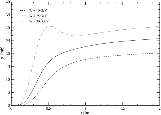
Figure 1: The FKS dipole cross section at $W=10,75,300$ GeV.

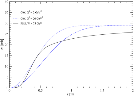
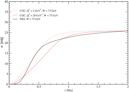
Figure 2: The GW dipole cross-section (left) and CGC dipole cross-section (right) at $W=75$ GeV for $Q^{2}=2~{}\mbox{GeV}^{2}$ and $Q^{2}=20~{}\mbox{GeV}^{2}$. The $Q^{2}$-independent FKS dipole cross-section at the same energy is shown for comparison.

2.2 The GW model

This well-known model [6, 7] combines the approximate behaviour $\hat{\sigma}\rightarrow r^{2}f(x)$ at small $r$ together with a phenomenological saturation effect by adopting the attractively simple parametric form:

$$\hat{\sigma}=\sigma_{0}\left(1-\exp\left[\frac{-r^{2}Q_{0}^{2}}{4(x_{\mathrm{mod}}/x_{0})^{\lambda}}\right]\right)\;.$$ (8)

Here $x_{\mathrm{mod}}$ is a modified Bjorken variable,

$$x_{\mathrm{mod}}=x\left(1+\frac{4m_{f}^{2}}{Q^{2}}\right)\;,$$ (9)

where $m_{f}$ is the quark mass and $Q_{0}=1$ GeV. The $3$ free parameters $x_{0}$, $\sigma_{0}$ and $\lambda$ were successfully fitted to $F_{2}$ data. The four-flavour fit which we shall use in this paper yielded $\sigma_{0}=29.12~{}\mbox{mb}$, $\lambda=0.277$ and $x_{0}=0.41\times 10^{-4}$. The quark masses are chosen to be $0.14$ GeV for the light quarks and $1.5$ GeV for the charm quark. The model is also able to describe $F_{2}^{D(3)}$ data [7]. A recent refinement of the model takes into account corrections due to DGLAP evolution at large $Q^{2}$ [19], but these are rather small corrections and are not included here. Finally, all these results are obtained with a purely perturbative photon wavefunction, which is somewhat enhanced at large $r$-values by the use of a lighter quark mass than that used in the FKS model.

The resulting behaviour of the dipole cross-section is illustrated and compared to that of the FKS model in Figure 2.

2.3 The CGC model

The dipole model of Iancu, Itakura and Munier [8] can be thought of as a development of the Golec-Biernat–Wüsthoff saturation model. Though still largely a phenomenological parameterisation, the authors do claim that it contains the main features of the “color glass condensate” regime, where the gluon densities are high and non-linear effects become important. In particular, they take

$$\hat{\sigma} = 2\pi R^{2}{\cal N}_{0}\left(\frac{rQ_{s}}{2}\right)^{2\left[\gamma_{s}+\frac{\ln(2/rQ_{s})}{\kappa\lambda\ln(1/x)}\right]}\hskip 28.45274pt\mathrm{for}\hskip 28.45274ptrQ_{s}\leq 2$$ (10)

$$= 2\pi R^{2}\{1-\exp[-a\ln^{2}(brQ_{s})]\}\hskip 28.45274pt\mathrm{for}\hskip 28.45274ptrQ_{s}>2~{},$$

where the saturation scale $Q_{s}\equiv(x_{0}/x)^{\lambda/2}$ GeV. The coefficients $a$ and $b$ are uniquely determined by ensuring continuity of the cross-section and its first derivative at $rQ_{s}=2$. The leading order BFKL equation fixes $\gamma_{s}=0.63$ and $\kappa=9.9$. The coefficient ${\cal N}_{0}$ is strongly correlated to the definition of the saturation scale and the authors find that the quality of fit to $F_{2}$ data is only weakly dependent upon its value. For a fixed value of ${\cal N}_{0}$, there are therefore three parameters which need to be fixed by a fit to the data, i.e. $x_{0}$, $\lambda$ and $R$. In this paper, we take $N_{0}=0.7$ and a light quark mass of $m_{q}=140$ MeV, for which the fit values are $x_{0}=2.67\times 10^{-5}$, $\lambda=0.253$ and $R=0.641$ fm.

As for the GW dipole, we compare to the FKS dipole at two values of $Q^{2}$ in Figure 2.

3 Light-cone wavefunctions

The light-cone wavefunctions $\Psi_{h,\bar{h}}(\bm{r},z)$ in the mixed representation $(r,z)$ used in the dipole model are obtained from a two dimensional Fourier transform

$$\Psi_{h,\bar{h}}(r,z)=\int\frac{d^{2}\bm{k}}{(2\pi)^{2}}e^{i\bm{k}\cdot\bm{r}}\;\Psi_{h,\bar{h}}(k,z)$$ (11)

of the momentum space light-cone wavefunctions $\Psi_{h,\bar{h}}(k,z)$, where the quark and antiquark are in states of definite helicity, $h$ and $\bar{h}$ respectively. For transversely ($T$) or longitudinally ($L$) polarised photons, the momentum space light-cone wave functions themselves are calculated perturbatively [9, 20] (per fermion of charge $ee_{f}$):

$$\Psi^{\gamma(\lambda)}_{h,\bar{h}}(k,z)=\sqrt{\frac{N_{c}}{4\pi}}\frac{\bar{u}_{h}(\bm{k})}{\sqrt{z}}(ee_{f}\gamma.\varepsilon_{\gamma}^{\lambda})\frac{v_{\bar{h}}(-\bm{k})}{\sqrt{1-z}}\Phi^{\gamma}(k,z)\;.$$ (12)

Hereafter, $\lambda$ denotes the polarization state $L$ or $T$. $\varepsilon^{\lambda}$ are the polarisation vectors and the “scalar” part of the photon light-cone wavefunction, $\Phi^{\gamma}$, is given by

$$\Phi^{\gamma}(k,z)=\frac{z(1-z)}{z(1-z)Q^{2}+k^{2}+m_{f}^{2}}\;.$$ (13)

For the vector mesons, the simplest approach is to assume the same vector current as in the photon case, with an additional (unknown) vertex factor $\Gamma_{\lambda}(k,z)$:

$$\Psi^{V(\lambda)}_{h,\bar{h}}(k,z)=\sqrt{\frac{N_{c}}{4\pi}}\frac{\bar{u}_{h}(\bm{k})}{\sqrt{z}}(\gamma.\varepsilon^{\lambda}_{V})\frac{v_{\bar{h}}(-\bm{k})}{\sqrt{1-z}}\Phi^{V}_{\lambda}(k,z)$$ (14)

where the scalar part of the meson light-cone wavefunction is given by

$$\Phi^{V}_{\lambda}(k,z)=\frac{z(1-z)\Gamma_{\lambda}(k,z)}{-z(1-z)M_{V}^{2}+k^{2}+m_{f}^{2}}\;.$$ (15)

Different models are defined by specifying these scalar wavefunctions. In practice, it is common to choose the same functional form for $\Phi^{V}_{T}$ and $\Phi^{V}_{L}$; perhaps allowing the numerical parameters to differ.

It is instructive to consider the longitudinal wavefunctions more explicitly. Using the polarisation vectors

$$\varepsilon_{\gamma}^{L}=\left(\frac{q^{+}}{Q},\frac{Q}{q^{+}},\bm{0}\right)\hskip 14.22636pt;\hskip 14.22636pt\varepsilon_{V}^{L}=\left(\frac{v^{+}}{M_{V}},-\frac{M_{V}}{v^{+}},\bm{0}\right)$$ (16)

and the rules of light-cone perturbation theory given in [20], it follows that the longitudinal photon light-cone wavefunction is

$$\Psi_{h,\bar{h}}^{\gamma,L}(k,z)=\sqrt{\frac{N_{c}}{4\pi}}\delta_{h,-\bar{h}}ee_{f}\left(\frac{2z(1-z)Q}{k^{2}+m_{f}^{2}+z(1-z)Q^{2}}-\frac{1}{Q}\right)\;.$$ (17)

and that of the vector meson is

$$\Psi^{V,L}_{h,\bar{h}}(k,z)=\sqrt{\frac{N_{c}}{4\pi}}\delta_{h,-\bar{h}}\left(\frac{z(1-z)2M_{V}\Gamma(k,z)}{k^{2}+m_{f}^{2}-z(1-z)M_{V}^{2}}+\frac{\Gamma(k,z)}{M_{V}}\right)\;.$$ (18)

On substituting (17) in (11) the second term of (17) leads to a dipole of vanishing size, which does not contribute to the cross-section. This is in accord with gauge invariance. The same argument cannot be used to justify the omission of the second term in the meson wavefunction (18), since the latter has a $k$ dependence. In practice, this term is omitted in the DGKP model [9], but retained in the NNPZ model [10]. A discussion of the gauge invariance issues surrounding this point can be found in [21].

Before discussing these models more fully, we give the explicit forms for the photon wavefunctions in $r$-space.

The normalised photon light-cone wavefunctions are [9]:

$$\Psi^{L}_{h,\bar{h}}(r,z)=\sqrt{\frac{N_{c}}{4\pi}}\delta_{h,-\bar{h}}ee_{f}2z(1-z)Q\frac{K_{0}(\epsilon r)}{2\pi}\;,$$ (19)

and

$$\Psi^{T(\gamma=\pm)}_{h,\bar{h}}(r,z)=\pm\sqrt{\frac{N_{c}}{2\pi}}ee_{f}\big{[}ie^{\pm i\theta_{r}}(z\delta_{h\pm,\bar{h}\mp}-(1-z)\delta_{h\mp,\bar{h}\pm})\partial_{r}+m_{f}\delta_{h\pm,\bar{h}\pm}\big{]}\frac{K_{0}(\epsilon r)}{2\pi}\;,$$ (20)

where

$$\epsilon^{2}=z(1-z)Q^{2}+m_{f}^{2}~{}.$$ (21)

Since the modified Bessel function $K_{0}(x)$ decreases exponentially at large $x$, these equations imply that at high $Q^{2}$, the wavefunctions are suppressed for large $r$ unless $z$ is close to its end-points values $0$ or $1$. As can be seen from equations (19)–(20), these end-points are suppressed for the longitudinal but not the transverse case. This is the origin of the statement that transverse meson production is more inherently non-perturbative than for longitudinal meson production.

For small $r$, the perturbative expressions given above are reliable. For large $r$-values, however, confinement corrections are likely to modify the perturbation theory result. These larger $r$-values contribute significantly at low $Q^{2}$, where the wavefunctions are sensitive to the non-zero quark masses $m_{f}$, which prevent the modified Bessel function from diverging in the photoproduction limit. For these reasons, the photon light-cone wavefunctions at large $r$ are clearly model-dependent.

We now turn back to the meson wavefunctions. These are subject to two constraints. The first is the normalisation condition [20, 22]

$$1=\sum_{h,\bar{h}}\int\frac{d^{2}\bm{k}}{(2\pi)^{2}}\,dz\,|\Psi^{V(\lambda)}_{h,\bar{h}}(k,z)|^{2}=\sum_{h,\bar{h}}\int d^{2}\bm{r}\,dz\,|\Psi^{V(\lambda)}_{h,\bar{h}}(r,z)|^{2}~{},$$ (22)

which embodies the assumption that the meson is composed solely of $q\bar{q}$ pairs. Note that this normalisation is consistent with equation (2) and differs by a factor $4\pi$ relative to the conventional light-cone normalisation.

The second constraint comes from the electronic decay width [9, 22]:

$$ef_{V}M_{V}\varepsilon_{\gamma}^{*}.\varepsilon_{V}=\sum_{h,\bar{h}}\int\frac{d^{2}\bm{k}}{(2\pi)^{2}}\frac{dz}{z(1-z)}(z(1-z)Q^{2}+k^{2}+m_{f}^{2})\Psi^{V}_{h,\bar{h}}(k,z)\Psi^{\gamma*}_{h,\bar{h}}(k,z)\;,$$ (23)

where the coupling $f_{V}$ of the meson to electromagnetic current can be determined from the experimentally measured leptonic width $\Gamma_{V\rightarrow e^{+}e^{-}}$ since $3M_{V}\Gamma_{V\rightarrow e^{+}e^{-}}=4\pi\alpha_{\mathrm{em}}^{2}f_{V}^{2}$. We shall prefer to implement the constraint directly in terms of the $r$-space wavefunctions. For our purposes, we can write the meson wavefunctions in $r$-space as

$$\Psi^{V,L}_{h,\bar{h}}(r,z)=\sqrt{\frac{N_{c}}{4\pi}}\delta_{h,-\bar{h}}\frac{1}{M_{V}z(1-z)}[z(1-z)M^{2}_{V}+\delta\times(m_{f}^{2}-\nabla_{r}^{2})]\phi_{L}(r,z)$$ (24)

where $\nabla_{r}^{2}\equiv\frac{1}{r}\partial_{r}+\partial^{2}_{r}$, and

$$\Psi^{V,T(\gamma=\pm)}_{h,\bar{h}}(r,z)=\pm\sqrt{\frac{N_{c}}{4\pi}}\frac{\sqrt{2}}{z(1-z)}[ie^{\pm i\theta_{r}}(z\delta_{h\pm,\bar{h}\mp}-(1-z)\delta_{h\mp,\bar{h}\pm})\partial_{r}+m_{f}\delta_{h\pm,\bar{h}\pm}]\phi_{T}(r,z).$$ (25)

Note the second term in square brackets which occurs in the longitudinal meson case. This is a direct consequence of keeping the second term in (18). For the DGKP wavefunctions this term is absent, i.e. $\delta=0$, whilst NNPZ keep this term, i.e. $\delta=1$. In terms of these wavefunctions, (23) becomes (assuming that $r\phi_{T}(r,z)\to 0$ at $r=0$ and $r=\infty$)

$$f_{V}M_{V}=\frac{N_{c}}{\pi}\hat{e}_{f}\int_{0}^{1}\frac{dz}{z(1-z)}\left.[z(1-z)M^{2}_{V}+\delta\times(m_{f}^{2}-\nabla_{r}^{2})]\phi_{L}(r,z)\right|_{r=0}$$ (26)

and

$$f_{V}M_{V}=-\frac{N_{c}}{2\pi}\hat{e}_{f}\int_{0}^{1}\frac{dz}{[z(1-z)]^{2}}\left.\left[(z^{2}+(1-z)^{2})\nabla_{r}^{2}-m_{f}^{2}\right]\phi_{T}(r,z)\right|_{r=0}.$$ (27)

In computing $f_{\phi}$ and all other observables involving the $\phi$ meson we in all cases take the quark mass to be equal to the light quark mass plus 150 MeV.

3.1 DGKP meson wavefunction

In the DGKP approach [9], the $r$ and $z$ dependence of the wavefunction are assumed to factorise. Specifically, the scalar wavefunction is given by

$$\phi_{\lambda}^{V}(r,z)=G(r)f_{\lambda}(z)z(1-z)$$ (28)

A Gaussian dependence on $r$ is assumed, that is

$$G(r)=\frac{\pi f_{V}}{N_{c}\hat{e}_{f}M_{V}}e^{-\frac{\omega^{2}_{\lambda}r^{2}}{2}}\;,$$ (29)

and $f_{\lambda}(z)$ is given by the Bauer-Stech-Wirbel model [24]:

$$f_{\lambda}(z)=\mathcal{N}_{\lambda}\sqrt{z(1-z)}e^{\frac{-M_{V}^{2}(z-1/2)^{2}}{2\omega^{2}_{\lambda}}}\;.$$ (30)

Setting $\delta=0$ (recall that this is equivalent to neglecting the second term in (18)) in (24) results in

$$\Psi_{h,\bar{h}}^{V,L}(r,z)=z(1-z)\delta_{h,-\bar{h}}\frac{\sqrt{\pi}f_{V}}{2\sqrt{N_{c}}\hat{e}_{f}}f_{L}(z)e^{-\omega_{L}^{2}r^{2}/2}\;,$$ (31)

for the DGKP longitudinal meson light-cone wavefunction. $\hat{e}_{f}$ is the effective charge arising from the sum over quark flavours in the meson: $\hat{e}_{f}=1/\sqrt{2},1/3$ and $2/3$ for the $\rho,~{}\phi$ and $J/\Psi$ respectively. Similarly, the DGKP transverse meson light-cone wavefunctions can be written as

$$\Psi_{h,\bar{h}}^{V,T(\gamma=\pm)}(r,z) = \pm\left(\frac{i\omega_{T}^{2}re^{\pm i\theta_{r}}}{M_{V}}[z\delta_{h\pm,\bar{h}\mp}-(1-z)\delta_{h\mp,\bar{h}\pm}]+\frac{m_{f}}{M_{V}}\delta_{h\pm,\bar{h}\pm}\right)$$ (32)

$$\hskip 142.26378pt\times\frac{\sqrt{\pi}f_{V}}{\sqrt{2N_{c}}\hat{e}_{f}}f_{T}(z)e^{-\omega_{T}^{2}r^{2}/2}\;.$$

The normalisation condition (22) on the DGKP wavefunction leads to the relations,

$$\omega_{\lambda}=\frac{\pi f_{V}}{\sqrt{2N_{c}}\hat{e}_{f}}\sqrt{I_{\lambda}}\;,$$ (33)

with

$$I_{L}=\int_{0}^{1}dzz^{2}(1-z)^{2}f_{L}^{2}(z)\;,$$ (34)

and

$$I_{T}=\int_{0}^{1}dz\frac{[z^{2}+(1-z)^{2}]\omega_{T}^{2}+m_{f}^{2}}{M_{V}^{2}}f_{T}^{2}(z)\;,$$ (35)

The leptonic decay width constraints (26) and (27) on the DGKP wavefunction yield

$$1=\int_{0}^{1}dz\;z(1-z)f_{L}(z)=\int_{0}^{1}dz\frac{2[z^{2}+(1-z)^{2}]\omega_{T}^{2}+m_{f}^{2}}{2M_{V}^{2}z(1-z)}f_{T}(z)\;.$$ (36)

The values of $\omega_{\lambda}$ and $\mathcal{N}_{\lambda}$ are found by solving (33) and (36) simultaneously, and are given in Table 2. The values of the decay constants used are the central experimental values [25]: $f_{\rho}=0.153\pm 0.004$ GeV, and $f_{\phi}=0.079\pm 0.001$ GeV.

Table 2

$$\begin{array}[]{c|c|c|c|l}\hline\cr\mbox{DGKP}&\omega_{L}&\omega_{T}&\mathcal{N}_{L}&~{}~{}~{}~{}\mathcal{N}_{T}\\ \hline\cr\rho&0.331&0.206,0.218&15.091&5.573,8.682\\ \phi&0.368&0.244,0.262&15.703&5.689,8.000\\ \hline\cr\end{array}$$

Table 2: Parameters and normalisations of the DGKP light-cone wavefunctions in appropriate GeV based units. For the transverse case, the first and second values are for the FKS and GW quark masses respectively.

The resulting behaviour of the $\rho$ wavefunctions is shown for the case of the FKS quark masses in Figures 3. As is clear from equations (28)–(32), the wavefunctions peak at $z=0.5$ and $r=0$, and go rapidly to zero as $z\rightarrow 0,1$ and $r\rightarrow\infty$, so that large dipoles are suppressed. From the figures, we see that the transverse wavefunction has a broader distribution than the longitudinal wavefunction. The $\phi$ wavefunctions are qualitatively similar to, but slightly more sharply peaked than, the $\rho$ wavefunctions.

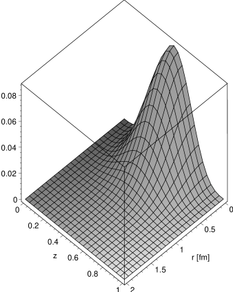
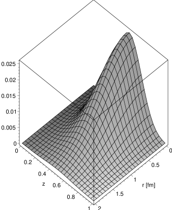
Figure 3: The $\rho$-wavefunctions $|\Psi^{L}|^{2}$ (left) and $|\Psi^{T}|^{2}$ (right) in the DGKP model with the quark mass used in the FKS dipole model. Note the different scales for the ordinate.

The GW model uses a much smaller value for the light quark masses than the FKS model, as we saw in Section 2.3. We might expect this to have a striking effect on the transverse wavefunction of the $\rho$, since the transverse wavefunction (32) vanishes at $r=0$ for zero quark masses, while the longitudinal wavefunction (31) does not. The transverse DGKP wavefunction with the light quark mass used in the GW dipole model is shown in Figure 4 for the $\rho$. As can be seen, the smaller quark mass decreases the wavefunction at the origin and shifts the peak to slightly larger $r$.

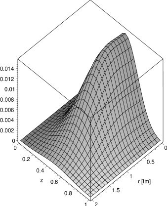
Figure 4: The $\rho$-wavefunction $|\Psi^{T}|^{2}$ in the DGKP model with the quark mass used in the GW dipole model.

3.2 Boosted wavefunctions

In this approach, the scalar part of the wavefunction is obtained by taking a given wavefunction in the meson rest frame. This is then “boosted” into a light-cone wavefunction using the Brodsky-Huang-Lepage prescription, in which the expressions for the off-shellness in the centre-of-mass and light-cone frames are equated [26] (or equivalently, the expressions for the invariant mass of the $q\bar{q}$ pair in the centre-of-mass and light-cone frames are equated [27]).

The simplest version of this approach assumes a simple Gaussian wavefunction in the meson rest frame. Alternatively NNPZ [10] have supplemented this by adding a hard “Coulomb” contribution in the hope of improving the description of the rest frame wavefunction at small $r$. We refer to [10] for details of this procedure. Here we simply state the result, which is that the NNPZ meson light-cone wavefunctions are given by equations (24, 25) with $\delta=1$, where the scalar wavefunctions $\phi_{\lambda}(r,z)$ are taken to be a sum of a soft (Gaussian in the rest frame) part and a hard (Coulomb) part:

$$\phi_{\lambda}(r,z) = \mathcal{N}_{\lambda}\ \left(4z(1-z)\sqrt{2\pi R^{2}}\exp\left(-\frac{m_{f}^{2}R^{2}}{8z(1-z)}\right)\exp\left(-\frac{2z(1-z)r^{2}}{R^{2}}\right)\right.$$ (37)

$$\left.\times\exp\left(\frac{m_{f}^{2}R^{2}}{2}\right)+16C^{4}\frac{a^{3}(r)}{A(r,z)B^{3}(r,z)}rK_{1}(A(r,z)r/B(r,z))\right).$$

Here

$$A(r,z)=\sqrt{1+\frac{C^{2}a^{2}(r)m_{f}^{2}}{z(1-z)}-4C^{2}a^{2}(r)m_{f}^{2}}\;,$$ (38)

$$B(r,z)=\frac{Ca(r)}{\sqrt{z(1-z)}}\;,$$ (39)

and

$$a(r)=\frac{3}{4m_{f}\alpha_{s}(r)}$$ (40)

is a running Bohr radius. The strong coupling $\alpha_{s}$ is chosen to run according to the prescription [28, 22]:

$$\alpha_{s}=\alpha_{0}~{}~{}\mbox{for}~{}~{}r>r^{s}~{}~{}~{}\mbox{and}~{}~{}\alpha_{s}(r)=\frac{4\pi}{\beta_{0}\log\left(1/(\Lambda_{\mbox{\tiny{QCD}}}^{2}r^{2})\right)}~{}~{}\mbox{for}~{}~{}r<r^{s}$$ (41)

where $r^{s}=0.42$ fm, $\alpha_{0}=0.8$, $\Lambda_{\mbox{\tiny{QCD}}}=0.2~{}\mbox{GeV}$ and $\beta_{0}=(33-2n_{f})/3$. Apart from the normalisation constants $\mathcal{N}_{\lambda}$ , these wavefunctions depend on two free parameters which are independent of the meson helicity: a “radius” parameter $R$ and a parameter $C$, introduced to control the transition between the hard Coulomb-like interaction and the soft confining interaction in the rest-frame wavefunction. The case of a simple Gaussian wavefunction in the rest-frame, which we will refer to as a “boosted Gaussian wavefunction” can be obtained by simply setting $C=0$ (we still choose $\delta=1$ when considering this wavefunction).

At this point we comment on two issues associated with the behaviour of the Coulomb part of the scalar wavefunction for small $r$. The first is that (37) diverges logarithmically as $r\rightarrow 0$ at $z=0.5$. This divergence is however regulated in observables. For example, while the resulting squared wavefunctions $|\Psi^{V(\lambda)}|^{2}$ exhibit a narrow, singular peak at $r=0,z=0.5$, the quantity $r|\Psi^{V(\lambda)}|^{2}$ which enters the normalisation condition (22) is zero in this limit. Nevertheless, this singular behaviour does have a (finite) effect when computing the meson decay constant which depends upon the behaviour of the wavefunction at $r=0$. The second issue is that when the scalar wavefunction (37) is substituted into equations (24) – (27), the derivatives in $r$ give rise to inverse power divergences at $r=0$ when acting upon the running coupling (41). However, these divergences occur solely in terms which are strictly higher order in $\alpha_{s}$. Henceforth we discard these higher order terms, which is equivalent to omitting all derivatives of $\alpha_{s}(r)$ with respect to $r$ when differentiating the scalar wavefunction (37). We stress that none of these issues arise when using the boosted Gaussian wavefunction.

It remains to determine the various constants. NNPZ [10] determined both $R$ and $C$ by using a standard variational procedure for the initial centre-of-mass wavefunction using a non-relativistic potential. They then checked that the resulting predictions (23) were in reasonable accord with the observed leptonic decay widths. Here we follow a slightly modified procedure, since we want to be able to easily adjust the quark masses to those assumed in the various dipole models. Specifically, we fixed $C$ at the value chosen by NNPZ and vary the value of $R$ to give approximate agreement with the decay width constraints (23). In practice, we found it adequate to use the same $R$-value for both the FKS and GW mass choices. The resulting values of $R$ and $C$, with the associated values of the normalisation constants, are shown in Table 3, and are not very different from the original parameters of NNPZ. In addition we show the results for the boosted Gaussian case ($C=0$) in Table 4.

Table 3

$$\begin{array}[]{c|c|c|c|c|c|c}\hline\cr\mbox{NNPZ}&R^{2}&C&\mathcal{N}_{L}&\mathcal{N}_{T}&f_{V}(L)&f_{V}(T)\\ \hline\cr\rho&25.0&0.36&0.0123,0.0121&0.0125,0.0137&0.143,0.147&0.157,0.109\\ \phi&18.0&0.53&0.0122,0.0124&0.0124,0.0131&0.078,0.078&0.087,0.067\\ \hline\cr\end{array}$$

Table 3: Parameters of the NNPZ light-cone wavefunctions in appropriate GeV based units, together with the resulting values for the decay constants $f_{V}$. Where two values are given, the first and second values are for the FKS and GW quark masses respectively.

Table 4

$$\begin{array}[]{c|c|c|c|c|c}\hline\cr\mbox{Gaussian}&R^{2}&\mathcal{N}_{L}&\mathcal{N}_{T}&f_{V}(L)&f_{V}(T)\\ \hline\cr\rho&12.3&0.0213,0.0244&0.0221,0.0259&0.153,0.161&0.203,0.192\\ \phi&10.0&0.0214,0.0243&0.0219,0.0251&0.075,0.079&0.095,0.088\\ \hline\cr\end{array}$$

Table 4: Parameters of the boosted Gaussian wavefunction in appropriate GeV based units, together with the resulting values for the decay constants $f_{V}$. Where two values are given, the first and second values are for the FKS and GW quark masses respectively.

The behaviour of the resulting $\rho$ wavefunctions is shown in Figures 5 with the FKS choice of quark masses. The divergence at $r=0,z=0.5$ is not visible since we do not plot down to $r=0$. Like the DGKP wavefunctions, they peak at $z=0.5$ and $r=0$, and go rapidly to zero as $z\rightarrow 0,1$ and $r\rightarrow\infty$. However, on comparing these figures with each other, and with Figures 3, two clear differences emerge.

Firstly, the peak in $z$ is less sharp in the boosted Gaussian case than in the DGKP and NNPZ cases.

Secondly, the large difference between the longitudinal and transverse wavefunctions found in the DGKP case is much less marked in the NNPZ and boosted Gaussian wavefunctions. In both cases, the peak in the transverse wavefunction is still broader than that in the longitudinal wavefuction, but it is a small effect in comparison with the DGKP case. This presumably reflects the fact that in the NNPZ and boosted Gaussian wavefunctions, the parameter $R$ has the same value for both helicities, since both wavefunctions are generated from the same non-relativistic wavefunction by the Brodsky-Huang-Lepage procedure.

Figures 6 show the wavefunctions in the case of the boosted Gaussian wavefunction.

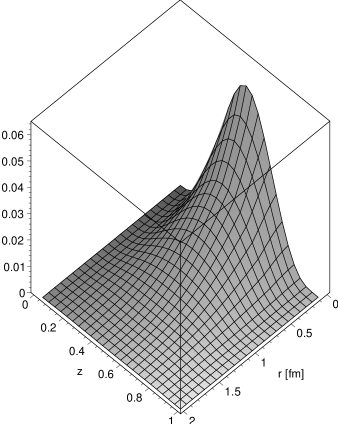
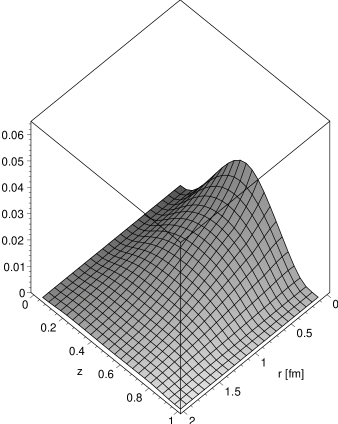
Figure 5: The $\rho$-wavefunctions $|\Psi^{L}|^{2}$ (left) and $|\Psi^{T}|^{2}$ (right) in the NNPZ model with the quark mass used in the FKS dipole model.

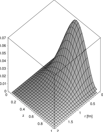
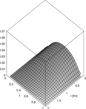
Figure 6: The $\rho$-wavefunctions $|\Psi^{L}|^{2}$ (left) and $|\Psi^{T}|^{2}$ (right) in the boosted Gaussian model with the quark mass used in the FKS dipole model.

4 Real parts, slope parameters and cross-sections

We now have all the ingredients required to calculate the absorptive parts (2) of the forward amplitudes for vector meson production. For the case of the NNPZ wavefunctions, we substitute the photon wavefunctions (19), (20) and the vector meson wavefunctions (24), (25) with $\delta=1$ into (2). Summing over the quark/antiquark helicities and averaging over the transverse polarisation states of the photon, we obtain:

$$\Im\mbox{m}\mathcal{A}^{L}_{\mbox{\tiny{NNPZ}}} = s\frac{N_{c}\hat{e}_{f}\sqrt{4\pi\alpha_{{\mathrm{em}}}}}{(2\pi)^{2}}\frac{2Q}{M_{V}}\int d^{2}\bm{r}\,\hat{\sigma}(s,r)\,\int_{0}^{1}dz$$ (42)

$$\left\{[m_{f}^{2}+z(1-z)M_{V}^{2}]K_{0}(\epsilon r)\phi_{L}(r,z)-K_{0}(\epsilon r)\nabla_{r}^{2})\phi_{L}(r,z)\right\}$$

$$\Im\mbox{m}\mathcal{A}^{T}_{\mbox{\tiny{NNPZ}}} = s\frac{N_{c}\hat{e}_{f}\sqrt{4\pi\alpha_{{\mathrm{em}}}}}{(2\pi)^{2}}\int d^{2}\bm{r}\,\hat{\sigma}(s,r)\,\int_{0}^{1}\frac{dz}{z(1-z)}$$ (43)

$$\left[(z^{2}+(1-z)^{2})\partial_{r}K_{0}(\epsilon r)\partial_{r}\phi_{T}(r,z)+m_{f}^{2}K_{0}(\epsilon r)\phi_{T}(r,z)\right]\;,$$

where $\phi_{L,T}(r,z)$ are given by (37). Similarly, using the DGKP wavefunctions (31) and (32), we obtain [9]

$$\Im\mbox{m}\mathcal{A}^{L}_{\mbox{\tiny{DGKP}}}=s\int d^{2}\bm{r}\,\hat{\sigma}(s,r)\int_{0}^{1}dz\sqrt{\frac{\alpha_{\mathrm{em}}}{4\pi}}f_{V}z(1-z)f_{L}(z)e^{-\omega_{L}^{2}r^{2}/2}2z(1-z)QK_{0}(\epsilon r)\;,$$ (44)

$$\Im\mbox{m}\mathcal{A}^{T}_{\mbox{\tiny{DGKP}}} = s\int d^{2}{\bm{r}}\,\hat{\sigma}(s,r)\int_{0}^{1}dz\sqrt{\frac{\alpha_{{\mathrm{em}}}}{4\pi}}f_{V}f_{T}(z)e^{-\omega_{T}^{2}r^{2}/2}$$ (45)

$$\left(\frac{\omega_{T}^{2}\epsilon r}{M_{V}}[z^{2}+(1-z)^{2}]K_{1}(\epsilon r)+\frac{m_{f}^{2}}{M_{V}}K_{0}(\epsilon r)\right)\;.$$

So far, we have focussed on the imaginary amplitude. Taking into account the real part contribution, the differential cross-section is given by

$$\left.\frac{d\sigma^{T,L}}{dt}\right|_{t=0}=\frac{1}{16\pi s^{2}}|\Im\mbox{m}\mathcal{A}^{T,L}|^{2}(1+\beta^{2})\;$$ (46)

where $\beta$ is the ratio of real to imaginary parts of the amplitude. It is most straightforward to reconstruct the real part of the amplitude in the FKS dipole model, where the dipole cross-section (3), and hence the amplitude (2), is given as the sum of hard and soft Regge pole terms. In this case, the real part is given by

$$\Re\mbox{e}\mathcal{A}_{\mbox{\tiny{FKS}}}=-\Im\mbox{m}\mathcal{A}_{\mbox{\tiny{soft}}}\cot\left(\frac{\pi\alpha_{S}}{2}\right)-\Im\mbox{m}\mathcal{A}_{\mbox{\tiny{hard}}}\cot\left(\frac{\pi\alpha_{H}}{2}\right)\;,$$ (47)

where $\alpha_{S,H}=1+\lambda_{S,H}=1.06,1.44$ and $\Im\mbox{m}\mathcal{A}_{\mbox{\tiny{soft}}}$ and $\Im\mbox{m}\mathcal{A}_{\mbox{\tiny{hard}}}$ are the contributions from the soft and hard Pomeron pieces of FKS dipole cross-section (3) respectively.

It follows from (47) that, in the FKS model, $\beta$ lies between 0.09 and 0.83, corresponding to pure soft and hard pomeron dominance respectively; within this range, the value of $\beta$ reflects directly the relative importance of the hard pomeron. Other things being equal, $\beta$ will therefore increase with increasing energy, because the hard term in the dipole cross-section increases more rapidly with energy than the soft term. It will also increase with $Q^{2}$, because the hard term is dominant for small dipoles, which are increasingly explored as $Q^{2}$ increases. These features are illustrated in Figure 7, which shows the values of $\beta$ obtained as functions of $W$ and $Q^{2}$ obtained using the DGKP wavefunctions. Here we also see that $\beta$ is larger for the longitudinal than for the transverse case, reflecting sharper peaking of the longitudinal vector meson wavefunctions. Similar results for the real parts are obtained using the NNPZ wavefunctions.

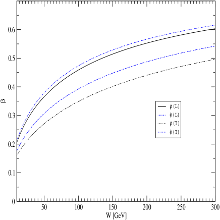
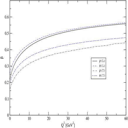
Figure 7: Left: $W$-dependence of the ratio $\beta$ of the real to imaginary part of the forward amplitude in the FKS model, using the DGKP wavefunctions, for $Q^{2}=10$ GeV². Right: $Q^{2}$-dependence of $\beta$ in the FKS model, using the DGKP wavefunctions, for $W=75$ GeV.

From the above figures, we see that while the corrections from the real parts in the cross-section formulae (46) are clearly significant in some kinematic ranges, they are nowhere dominant. Because of this and because the ratio $\beta$ is expected to be similar in the different models, we shall use the estimates (47) of the ratio $\beta$ obtained in the FKS model in both dipole models.

Assuming the usual exponential ansatz for the $t$ dependence, the total cross-sections are given by

$$\sigma^{T,L}(\gamma^{*}p\rightarrow Vp)=\frac{d\sigma^{T,L}/dt|_{t=0}}{B}\;.$$ (48)

Unfortunately, the values of the slope parameter $B$ are not very accurately measured. Here we use a parametrisation

$$B=0.60\left(\frac{14}{(Q^{2}+M_{V}^{2})^{0.26}}+1\right)$$ (49)

obtained from a fit to experimental data by Mellado [29], and used in their analysis of the predictions of the GW dipole model by Caldwell and Soares [30]. The resulting values for $B$ are shown in Figure 8, where we also show the results of an alternative parameterisation of Kreisel [31] to illustrate the range of values that can be obtained from different fits to the data. When comparing the predictions of (48) for the vector meson cross-sections with data, it is important to bear in mind that this uncertainty in the input value of the slope parameter can easily introduce errors up to of order 30$\%$ or so and that, within this range, this error may be $Q^{2}$ dependent.

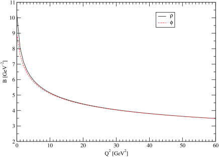
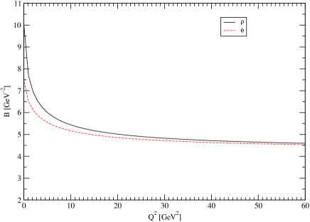
Figure 8: Left: Parametrisation of the slope $B$ by Mellado [29] for the $\rho$ and $\phi$. Right: Parametrisation of the slope $B$ by Kreisel [31] for the $\rho$ and $\phi$.

Finally, on comparing with experimental data, we show $\sigma^{\mbox{\tiny{TOT}}}=\sigma^{T}+\epsilon\sigma^{L}$ with $\epsilon=0.98$ in all our plots, although the HERA data range from 0.96 to 1.00.

5 Results

In this section we will compare the predictions of the three dipole models with the experimental data for our three choices of vector meson wavefunction, without any adjustment of parameters. Before doing so, however, we emphasize again that the uncertainty in the slope parameter can give rise to $Q^{2}$-dependent errors of up to 30$\%$ in the cross-section, which should be borne in mind when comparing with experiment. This effect should, hopefully, be much smaller in the ratio $R$. However, it ought not to be completely negligible since the longitudinal and transverse cross-sections will presumably have slightly different slope parameters, as to some degree they explore dipoles of different sizes.

5.1 $\rho$ meson production

The predictions of the FKS model for the $Q^{2}$ dependence of the cross-section and for the longitudinal to transverse ratio $R$ are shown in Figure 9 for the three different wavefunctions considered. The equivalent plots for the GW and CGC model are in Figures 10 and 11 respectively.

The ZEUS total cross-section data are at the following centre-of-mass energies: 0.27 GeV${}^{2}<Q^{2}<$ 0.69 GeV², $W=51.1$ GeV, otherwise $W=75$ GeV. The H1 data on the longitudinal to transverse ratio are, for $Q^{2}=9.8,~{}18.25$ GeV², in the range 40 GeV $<W<$ 140 GeV, otherwise they are at $W=75$ GeV. Similarly the ZEUS data are, for $Q^{2}=0.33$ GeV², at $W=67$ GeV or for $Q^{2}=0.62$ GeV² at $W=47$ GeV. For the theory curves we always take $W=75$ GeV.

For all three dipole models, the data favour the boosted Gaussian wavefunction, whilst the DGKP wavefunction produces reasonable agreement for FKS and is rather less satisfactory for the GW and CGC models. The NNPZ wavefunction is well below the total cross-section data for all three models and, for the GW and CGC models, in disagreement with the data on the longitudinal to transverse ratio. However, as noted in section 3.2, although the spurious singularity in this wavefunction does not contribute directly to the predicted cross-sections, it influences them indirectly because it influences the value of the radial parameter $R$ deduced from the decay width. In what follows, we will therefore focus on the DGKP and boosted Gaussian wavefunctions.

Figures 12, 13 and 14 show the $W$ dependence at fixed values of $Q^{2}$ for the $\rho$ meson. Apart from the normalisation, the $W$-dependence is good in all cases. The normalisation is best described by the boosted Gaussian wavefunction. With this wavefunction, the FKS model is in reasonably good agreement with the data, except for the ZEUS data at very low $Q^{2}$; while the GW and CGC models give reasonable agreement everywhere.

This last comment contrasts somewhat with the work of Caldwell and Soares [30], who have already presented predictions for the GW model using a boosted Gaussian wavefunction. These authors also found good agreement with the data on the longitudinal to transverse ratio and with the $W$ dependence at fixed $Q^{2}$ apart from the normalisation. However their results for the normalisation, and hence, implicitly, for the $Q^{2}$-dependence of the production cross-section, were relatively poor. However, these authors did not implement the leptonic decay width constraint but fixed the radial parameter $R$ in the boosted Gaussian by requiring that the exponential in $R$ of the wavefunction gives a value of $1/e$ when the $q\bar{q}$ invariant mass is equal to the meson’s mass. This yielded $R^{2}=15.5~{}\mbox{GeV}^{-2}$ for $\rho$ and $R^{2}=8.3~{}\mbox{GeV}^{-2}$ for $\phi$ compared to our values shown in Table 4. In addition, they neglected real parts, which can result in a 20$\%$ reduction in the cross-section for large $Q^{2}$.

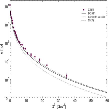
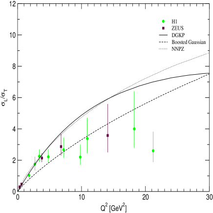
Figure 9: The $Q^{2}$ dependence of left the total cross-section and right the longitudinal to transverse cross-section ratio for $\rho$ production at $W=75$ GeV in the FKS model using the three different meson wavefunctions. Data from left [32] and right [32, 33].

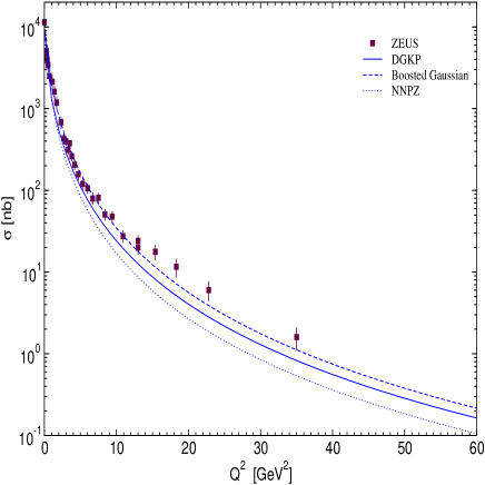
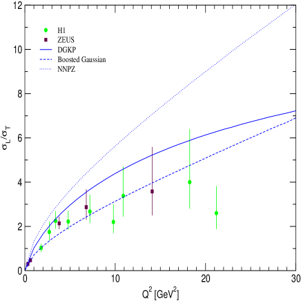
Figure 10: The $Q^{2}$ dependence of left the total cross-section and right the longitudinal to transverse cross-section ratio for $\rho$ production at $W=75$ GeV in the GW model using the three different meson wavefunctions. Data from left [32] and right [32, 33].

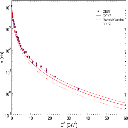
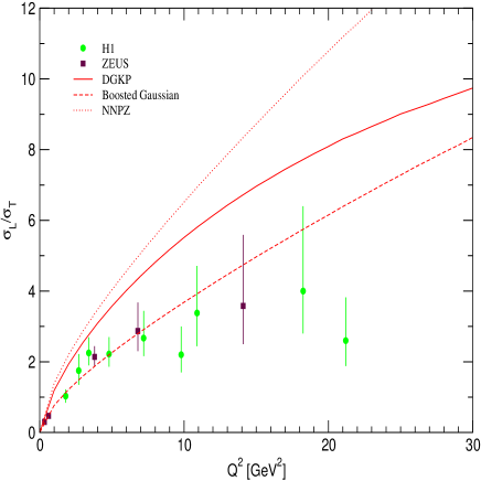
Figure 11: The $Q^{2}$ dependence of left the total cross-section and right the longitudinal to transverse cross-section ratio for $\rho$ production at $W=75$ GeV in the CGC model using the three different meson wavefunctions. Data from left [32] and right [32, 33].

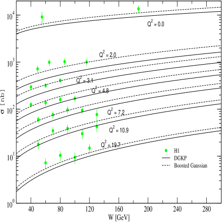
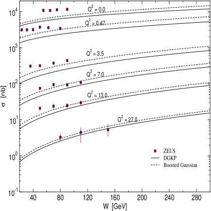
Figure 12: The $W$ dependence of the total cross-section for $\rho$ production at various values of $Q^{2}$. We use the FKS dipole model and compare the boosted Gaussian and DGKP wavefunctions. Data from left [34] and right [32].

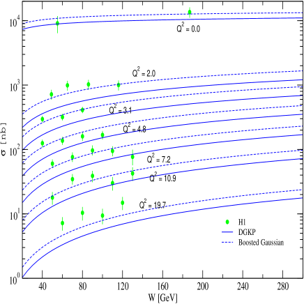
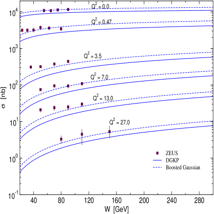
Figure 13: The $W$ dependence of the total cross-section for $\rho$ production at various values of $Q^{2}$. We use the GW dipole model and compare the boosted Gaussian and DGKP wavefunctions. Data from left [34] and right [32].

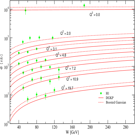
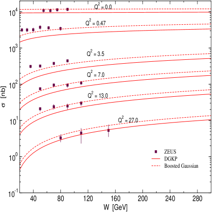
Figure 14: The $W$ dependence of the total cross-section for $\rho$ production at various values of $Q^{2}$. We use the CGC dipole model and compare the boosted Gaussian and DGKP wavefunctions. Data from left [34] and right [32].

5.2 $\phi$ meson production

The corresponding plots to those in the previous section are repeated for the $\phi$ meson in Figures 15, 16 and 17. The H1 total cross-section data are at the following centre-of-mass energies: for $Q^{2}=7.5,8.3,12.5,14.6,17.3$ GeV², $W=100$ GeV, otherwise $W=75$ GeV. Similarly for the ZEUS data, for $Q^{2}=0.0,8.2,14.7$ GeV², $W=70,94,99$ GeV respectively. The H1 data on the longitudinal to transverse ratio are in the range 40 GeV $<W<$ 130 GeV. Similarly the ZEUS data are in the range 25 GeV $<W<120$ GeV. For the theory curves we always take $W=90$ GeV.

The situation is rather similar, as one might expect, to that of the $\rho$, i.e. all three dipole models tend to do rather well with either of the DGKP or boosted Gaussian wavefunctions, while the NNPZ wavefunction is less satisfactory.

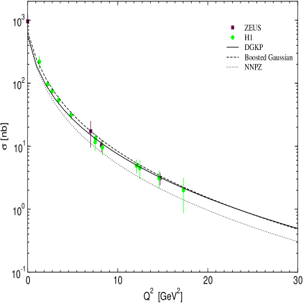
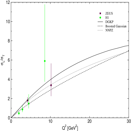
Figure 15: The $Q^{2}$ dependence of left the total cross-section and right the longitudinal to transverse cross-section ratio for $\phi$ production at $W=90$ GeV in the FKS model using the three different meson wavefunctions. Data from left [35, 36] and right [37, 38].

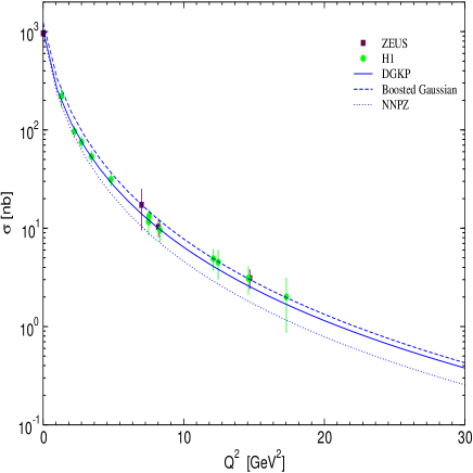
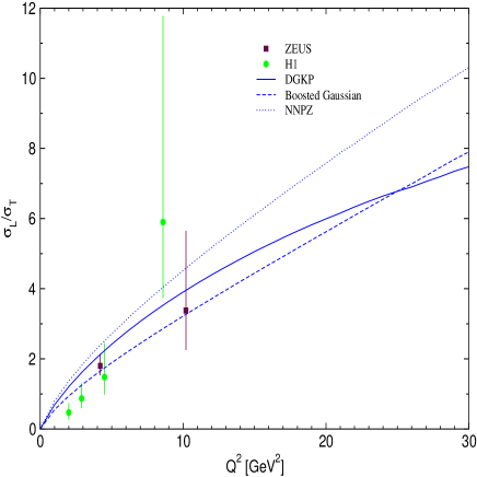
Figure 16: The $Q^{2}$ dependence of left the total cross-section and right the longitudinal to transverse cross-section ratio for $\phi$ production at $W=90$ GeV in the GW model using the three different wavefunctions. Data from left [35, 36] and right [37, 38].

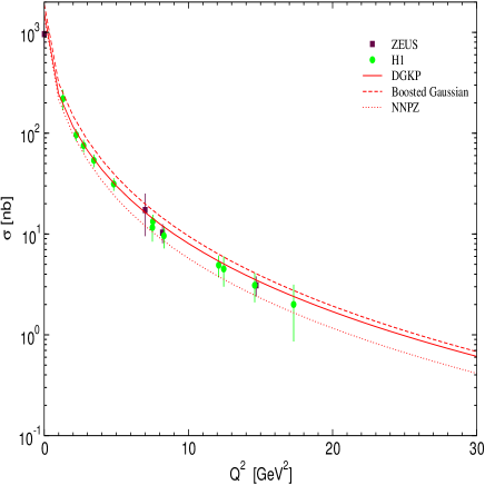
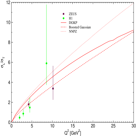
Figure 17: The $Q^{2}$ dependence of left the total cross-section and right the longitudinal to transverse cross-section ratio for $\phi$ production at $W=90$ GeV in the CGC model using the three different wavefunctions. Data from left [35, 36] and right [37, 38].

6 Conclusions

We have performed a detailed study, comparing the predictions on $\rho$ and $\phi$ meson electroproduction arising from three different models of the meson wavefunction in combination with three different models for the fundamental dipole cross-section. Our results are broadly encouraging and support the use of the dipole approach.

The data can be explained rather well using the dipole model of Forshaw, Kerley and Shaw, or those of Golec-Biernat and Wüsthoff and of Iancu, Itakura and Munier, in conjunction with either the boosted Gaussian or DGKP meson wavefunction. Certainly, we anticipate that excellent agreement could be obtained if one decided to tune the meson wavefunctions. Note that agreement extends to the ratio of longitudinal to transverse meson production. The NNPZ wavefunction, which has, as noted, an unphysical singularity at $z=0.5$, $r=0$, is not so successful.

For the future, it is clear that one could use the high quality data from HERA to constrain the meson wavefunctions provided the dipole cross-section is sufficiently constrained.

References

- [1] J. R. Forshaw, G. Kerley and G. Shaw, Phys. Rev. D60 (1999) 074012.
- [2] J. R. Forshaw, G. Kerley and G. Shaw, Nucl. Phys. A675 (2000) 80c.
- [3] M. McDermott, R. Sandapen and G. Shaw, Eur. Phys. J. C. 22 (2002) 655.
- [4] C. Adloff et al., H1 Collab., Z. Phys. C76 (1997) 613; J. Breitweg et al., ZEUS Collab., Eur. Phys. J. C6 (1999) 43.
- [5] C. Adloff et al., H1 Collab., Phys. Lett. B517 (2001) 47; S. Chekanov et al., Phys. Lett. B573 (2003) 46.
- [6] K. Golec-Biernat and M. Wüsthoff, Phys. Rev. D59 (1999)014017.
- [7] K. Golec-Biernat and M. Wüsthoff, Phys. Rev. D60 (1999) 114023.
- [8] E. Iancu, K. Itakura and S. Munier, hep -ph/0310338.
- [9] H. G. Dosch, T. Gousset, G. Kulzinger and H. J. Pirner, Phys. Rev. D55 (1997) 2602.
- [10] J. Nemchik, N. N. Nikolaev, E. Predazzi and B. G. Zakharov, Z.Phys. C75 (1997) 71.
- [11] N. N. Nikolaev and B. G. Zakharov, Z. Phys. C49 (1991) 607; Z. Phys. C53 (1992) 331; A. H. Mueller, Nucl. Phys. B415 (1994) 373; A. H. Mueller and B. Patel, Nucl. Phys. B425 (1994) 471.
- [12] M. McDermott, The dipole picture of small physics (A summary of the Amirim meeting), hep-ph/0008260v2.
- [13] L. Frankfurt, V. Guzey and M. Strikman, Phys. Rev. D58 (1998) 094039.
- [14] H. Fraas, B. J. Read and D. Schildknecht, Nucl. Phys. B86 (1975) 346.
- [15] G. Shaw, Phys. Rev. D47 (1993) R3676; G. Shaw, Phys. Lett. B228 (1989) 125; P. Ditsas and G. Shaw, Nucl.Phys. B113 (1976) 246.
- [16] G. Cvetic, D. Schildknecht, B. Surrow and M. Tentyukov, Eur. Phys. J. C20 (2001) 77.
- [17] L.V. Gribov, E.M. Levin and M.G. Ryskin, Phys. Rep. 100 (1983) 1.
- [18] J. R. Forshaw, G. Kerley, G. Shaw, Proc 8th Int. Workshop on Deep Inelastic Scattering, Eds. J. A. Gracey and T. Greenshaw, World Scientific, 2001. hep-ph/0007257.
- [19] J. Bartels, K. Golec-Biernat and H. Kowalski, Phys. Rev D66 (2002) 014001.
- [20] S. J. Brodsky and G. P. Lepage, Phys. Rev. D22 (1980) 2157.
- [21] A. Hebecker and P. V. Landshoff, Phys. Lett. B419 (1998) 393.
- [22] S. Munier, A. Mueller and A. Stasto, Nucl. Phys. B603 (2001) 427.
- [23] H. Halperin and A. Zhitnitsky, Phys. Rev. D56 (1997) 184.
- [24] M. Wirbel, B. Stech and M. Bauer, Z. Phys. C29 (1985) 637.
- [25] Particle data group: K. Hagiwara et al., Phys. Rev. D66 (2002) 010001.
- [26] S. J. Brodsky, T. Huang and G. P. LePage, SLAC-PUB-2540 (1980), Shorter version contributed to 20th Int. Conf. on High Energy Physics, Madison, Wisc., Jul 17-23, 1980.
- [27] A. Donnachie, J. Gravelis and G. Shaw, Phys. Rev. D63 (2001) 114013.
- [28] J. Nemchik, N. N. Nikolaev and B. G. Zakharov, Phys. Lett. B341 (1994) 228.
- [29] B. Mellado, unpublished result given in [30].
- [30] A. Caldwell and M. Soares, Nucl. Phys. A696 (2001) 125.
- [31] A. Kreisel, paper presented at LISHEP 02, hep-ex/020801v1.
- [32] J. Breitweg et al., ZEUS Collab., Eur. Phys. J. C6 (1999) 603.
- [33] S. Aid et al., H1 Collab., Nucl. Phys. B463 (1996) 3.
- [34] C. Adloff et al., H1 Collab., Eur. Phys. J. C13 (2000) 371; H1 Collab., Nucl. Phys. B468 (1996) 3.
- [35] C. Adloff et al., H1 Collab., Phys. Lett. B483 (2000) 360; Z. Phys. C75 (1997) 607.
- [36] M. Derrick et al., ZEUS Collab., Phys. Lett. 377B (1996) 259; Phys. Lett. B380 (1996) 220.
- [37] C. Adloff et al., H1 Collab., Phys. Lett. B483 (2000) 360.
- [38] ZEUS Collaboration, submitted paper 793 to ICHEP 98.