Baryon Form Factors of Relativistic Constituent-Quark Models

Abstract

The electromagnetic and axial form factors of the nucleon and its lowest positive parity excitations, the $\Delta(1232)$ and the $N(1440)$, are calculated with constituent-quark models that are specified by simple algebraic representations of the mass-operator eigenstates. Poincaré covariant current operators are generated by the dynamics from single-quark currents that are covariant under a kinematic subgroup. The dependence of the calculated form factors on the choice of kinematics and on the gross features of the wave functions is illustrated for instant-form, point-form, and front-form kinematics. A simple algebraic form of the orbital ground state wave function, which depends on two parameters, allows a fair description of all the form factors over the empirically accessible range, although with widely different choices of the parameters, which determine the range and shape of the orbital wave function. The neutron electric form factor requires additional features, for instance the presence of mixed symmetry $S-$state component with 1 – 2 % probability in the ground state wave function. Instant and front form kinematics demand a spatially extended wave function, whereas in point form kinematics the form factors may be described with a quite compact wave function.

I Introduction

The baryon states of constituent-quark models are represented by functions of three quark coordinates, spin, flavor and color variables. The Hilbert space of states is the tensor product of three irreducible Poincaré representations. The bound state wave functions represent vectors in the representation space of the little group of the Poincaré transformations. A calculation of baryon form factors requires consistent representations of the current-density operators and the baryon states. While current density operators are represented by functions of quark velocities and spinor indices, the baryon states are represented by eigenfunctions of the mass operator, which are functions of internal momenta, $\vec{k}_{i}$, and spin variables. The relation between the two representations depends on the “form of kinematics”, which specifies a kinematic subgroup of the Poincaré group.

Following Bakamjian and Thomas bakam the baryon states may be represented by eigenfunctions of the mass operator, ${\cal M}$, the spin operator, $j^{2},j_{z}$, and three kinematic operators which, together with the mass operator, specify the four-momentum. The mass operator commutes with these operators and is independent of their eigenvalues, which therefore may be treated as parameters. Relevant examples are the velocity $\vec{v}$, the three-momentum $\vec{P}$, and the light-front momentum ${\bf P}:=\{P^{+},P_{\perp}\}$, with the four-momentum represented respectively by

$$P={\cal M}\left\{\sqrt{1+|\vec{v}|^{2}},\vec{v}\right\}\;,\qquad P=\left\{\sqrt{|\vec{P}|^{2}+{\cal M}^{2}},\vec{P}\right\}\;,\qquad P=\left\{{{\cal M}^{2}+P_{\perp}^{2}\over P^{+}},{\bf P}\right\}\;.$$ (1)

The choice of these kinematic parameters implies the “form of kinematics”, which is the choice of a kinematic subgroup of the Poincaré group coe02 . The Poincaré representations of the kinematic subgroup are independent of the mass operator. In particular, they are the same as the representations of free quarks with mass operator ${\cal M}_{0}$. The kinematic subgroups, which correspond to the momentum representations in Eq. (1) are the Lorentz group, $SO(1,3)$, the Euclidean group in three dimensions $E(3)$ (translations and rotations at a fixed time), and the symmetry group of the null-plane $n\cdot x=0,\;n^{2}=0$. Following Dirac’s seminal paper dirac , the three forms of kinematics are referred to as point form, instant form and front form.

The relations between the internal momenta and spin variables to the quark velocities and spinor variables depend on boost parameters which are $\vec{v}$, $\vec{P}$ and $P_{\perp}/P^{+}$, with Lorentz kinematics, instant kinematics and light-front kinematics, respectively. Poincaré covariant current-density operators can be generated by the dynamics from current operators that are covariant under the kinematic subgroup only. Employment of free-quark currents for that purpose leads to different current operators in the different forms of kinematics. The quark masses enter as essential scale parameters of these current operators.

While the mass operator of conventional quark models, e.g. boffi , also depends on the quark masses, baryon spectra of confined quark may be represented by mass operators that are independent of quark masses coe98 . Eigenfunctions of such mass operators can be consistent with empirical nucleon form factors coe03 . Nucleon models constructed in this manner depend only on one scale that can be varied by unitary transformations. Form factors are dimensionless functions of the invariant velocity difference $\eta:=1/4(v_{out}-v_{in})^{2}$, and the mass ratio $M_{out}/M_{in}$. With Lorentz kinematics $\eta$ is a kinematic quantity and the form factors are relatively insensitive to unitary scale transformations of the wave function. Relations to momentum transfers involve the baryon masses. With instant and light-front kinematics momentum transfers are kinematic, since for these there is kinematic translation covariance in 3 or 2 space dimensions respectively.

Poincaré covariant state vectors of few-body systems are represented by equivalence classes of functions polyzou and there is no relation of a particular representation to wave functions defined by matrix elements of field operators desplanques ; brodsky .

The purpose of this paper is to explore the dependence of the baryon elastic and transition form factors on the representation of the baryon mass operator and on the form of kinematics used in the construction of the current operators. For that purpose we assume a Bakamjian-Thomas representation of the baryon states and generate current density operators from simple quark currents that are covariant under the kinematic subgroup only. Non-Bakamjian-Thomas representations of the baryon states are equivalent by unitary transformations, which modify the representation of the quark currents polyzou .

The mass operator is constructed in a simple spectral representation, which is independent of quark masses:

$$\langle{\sigma_{1},\sigma_{2},\sigma_{3},\vec{k}_{1},\vec{k}_{2},\vec{k}_{3}}|{\cal M}|{\sigma_{3}^{\prime},\sigma_{2}^{\prime},\sigma_{1}^{\prime},\vec{k}^{\prime}_{3},\vec{k}^{\prime}_{2},\vec{k}^{\prime}_{1}}\rangle$$ (2)

$$=\sum_{n,j,\sigma}\phi_{n,j,\sigma}(\sigma_{1},\sigma_{2},\sigma_{3},\vec{k}_{1},\vec{k}_{2},\vec{k}_{3})M_{n,j}\phi_{n,j,\sigma}(\sigma_{1}^{\prime},\sigma_{2}^{\prime},\sigma_{3}^{\prime},\vec{k}_{1}^{\prime},\vec{k}_{2}^{\prime},\vec{k}_{3}^{\prime})^{*}\,,$$ (3)

with the restriction to the nucleon, the $\Delta(1232)$ and the $N(1440)$. Generalization to other states is straightforward. A two-parameter family of algebraic functions is employed, which allow variations of the range and the shape of the function. Using hyperspherical coordinates, the spatial wave function of the $N(1440)$ baryon is constructed with a single node to be orthogonal to the ground state. For a satisfactory description of the electric form factor of the neutron a small admixture of $\sim$ 1–2 % of a mixed symmetry $S-$state is included in the ground state wave function.

For the quark currents the same structureless spinor currents are employed throughout. Variations of this input are beyond the scope of this article. The quark velocities are related to the internal momenta by boost relations, which depend on the choice of the kinematics with significant qualitative and quantitative consequences. With point-form and light-front kinematics different quark velocities are related by kinematic Lorentz transformations. With instant-form kinematics there is no kinematic relation between different quark velocities. With light-front and instant form kinematics translation covariance emphasizes the spatial extent, $r_{0}$, of the wave function.

When the spatial extent of the wave function is scaled unitarily to zero, the calculated form factors become independent of momentum transfer in both instant and front form kinematics. In contrast point form kinematics has a non-trivial limit, when the spatial extent of the wave function is scaled to zero. In this “point limit” the calculated form factors depend on the functional form of the wave function, and when $\eta\gg 1$ decrease with an inverse power of the momentum transfer. The falloff power is determined by the current operator and is independent of the wave function coe03 .

The present paper is organized in the following way. In Section II the model independent relations of covariant current matrices to invariant form factors are summarized. Section III contains the description of the baryon model specified by a mass operator and kinematic quark currents. Section IV contains a detailed description of the integrals which need to be evaluated after summation over spin and flavor indices. Numerical results are presented in Section V. A concluding discussion is given in Section VI.

II Current-density operators and form factors

The definition of form factors depends on the Poincaré covariance of the current density operators $I^{\mu}(x)$ and the basis states $|{M,v,j,j_{z}}\rangle$. The current density

$$I^{\mu}(x)=e^{iP\cdot x}I^{\mu}(0)e^{-iP\cdot x}\;,$$ (4)

satisfies the Lorentz covariance relations

$$U^{\dagger}(\Lambda)I^{\mu}(x)U(\Lambda)=\Lambda^{\mu}\,_{\nu}I^{\nu}(\Lambda^{-1}x)\;.$$ (5)

By definition the spin operator $\vec{j}$ is related to the Lorentz generators $J^{\mu\nu}$ by

$$\{0,\vec{j}\}:=B^{-1}(v)\,w\qquad\mbox{with}\qquad w_{\tau}:={\textstyle{1\over 2}}v^{\nu}J^{\rho\sigma}\epsilon_{\nu\rho\sigma\tau}$$ (6)

where the boost operator $B(v)$ is an operator valued Lorentz transformation with the defining property:

$$B(v)\{1,0,0,0\}=v\;.$$ (7)

It follows from the definition (6) and the Lorentz covariance of the velocity operator, $U^{\dagger}(\Lambda)\,v\,U(\Lambda)=\Lambda v$, that the spin operator transforms according to

$$U^{\dagger}(\Lambda)\,\vec{j}\,U(\Lambda)={\cal R}_{W}(\Lambda,v)\vec{j}\;,$$ (8)

with the Wigner rotations ${\cal R}_{W}(\Lambda,v)$ defined by

$${\cal R}_{W}(\Lambda,v):=B^{-1}(\Lambda v)\Lambda B(v)\,.$$ (9)

The basis states transform according to

$$U(\Lambda)|{M,v,j,\sigma}\rangle=\sum_{\sigma^{\prime}}|{M,\Lambda v,j,\sigma^{\prime}}\rangle D^{j}_{\sigma^{\prime},\sigma}[R_{W}(\Lambda,v)]\;.$$ (10)

With definite initial and final velocities and masses, $v_{a},M_{a}$ and $v_{f},M_{f}$ the form factors are determined by invariant reduced matrix elements of the currents. They are dimensionless functions of $\eta$:

$$\eta:={\textstyle{1\over 4}}(v_{f}-v_{a})^{2}\;,\qquad-{\textstyle{1\over 4}}(v_{f}+v_{a})^{2}=1+\eta\;,$$ (11)

and the baryon masses. The relation between the invariant momentum transfer and $\eta$ is:

$$Q^{2}:=(M_{f}v_{f}-M_{a}v_{a})^{2}=4M_{f}M_{a}\eta-(M_{f}-M_{a})^{2}\;.$$ (12)

In practice the dynamics generates the current operators from kinematic currents that are covariant under a subgroup only. It is therefore important to define basis states such that the Wigner rotations of kinematic transformations are kinematic. For Lorentz and instant kinematics canonical boosts satisfy this requirement. For any rotation ${\cal R}$ the corresponding Wigner rotation satisfies ${\cal R}_{W}({\cal R},v)={\cal R}$ and for rotationless Lorentz transformations in the direction of $\vec{v}$ the Wigner rotations reduce to the identity. Light-front kinematic requires null-plane boosts defined such that the Wigner rotations of null-plane boosts are the identity.

II.1 Electromagnetic form factors

Lorentz and instant kinematics share the subgroup of rotations about the direction of the velocities, which suggests the use of canonical spins and the separation of the conserved current density, $I^{\mu}(0)$, into “electric” and “magnetic” currents which are projections of the current into the plane defined by the velocities $v_{a}$ and $v_{f}$ and the projection perpendicular to that plane.

Current conservation, $(M_{f}v_{f}-M_{a}v_{a})\cdot I(0)=0$, implies that the electric current be a linear combination of the velocities multiplied by a single invariant operator ${\cal I}_{e}$. It is satisfied by the expression.

$$I^{\mu}_{e}(0)=\left\{{M_{f}+M_{a}\over\sqrt{4M_{f}M_{a}}}{v^{\mu}_{f}+v^{\mu}_{a}\over 2\sqrt{1+\eta}}+{M_{f}-M_{a}\over\sqrt{4M_{f}M_{a}}}{v^{\mu}_{f}-v^{\mu}_{a}\over 2\sqrt{\eta}}\sqrt{{1+\eta\over\eta}}\right\}{\cal I}_{e}\,,$$ (13)

which implies

$${\cal I}_{e}:=-{(M_{a}v_{f}+M_{f}v_{a})\over 2\sqrt{1+\eta}\sqrt{M_{a}M_{f}}}\cdot I(0)\,.$$ (14)

The choice of coordinate axes is a matter of convenience. When the z-axis is in the direction of the velocities, the components of the magnetic current are

$$I_{m}(0)=\{0,{\cal I}_{mx}(\eta),{\cal I}_{my}(\eta),0\}\,.$$ (15)

Electric and magnetic form factors are invariant matrix elements of the expressions (13) and (15). Both ${\cal I}_{e}$ and $\vec{\cal I}_{m}$ are invariant under rotationless Lorentz transformations in the z-direction and, with canonical boosts, the corresponding Wigner rotations are the identity. Form factors can thus be defined by invariant canonical-spin matrix elements.

The elastic form factors of the nucleon are defined by:

$$G_{E}(\eta) := \langle{{\textstyle{1\over 2}}}|{\cal I}_{e}(\eta)|{{\textstyle{1\over 2}}}\rangle_{c}=\langle{-{\textstyle{1\over 2}}}|{\cal I}_{e}(\eta)|{-{\textstyle{1\over 2}}}\rangle_{c}\;,$$ (16)

$$G_{M}(\eta) := {1\over\sqrt{\eta}}\langle{{\textstyle{1\over 2}}}|{\cal I}_{mx}(\eta)|{-{\textstyle{1\over 2}}}\rangle_{c}=-{1\over\sqrt{\eta}}\langle{-{\textstyle{1\over 2}}}|{\cal I}_{mx}(\eta)|{{\textstyle{1\over 2}}}\rangle_{c}\;.$$

The magnetic form factor for the transition between a spin 1/2 and a spin 3/2 state can be defined by:

$$G_{M{\textstyle{3\over 2}}}(\eta):={1\over\sqrt{\eta}}\bigg{[}\langle{{\textstyle{1\over 2}},{\textstyle{1\over 2}}}|{\cal I}_{mx}(\eta)|{{\textstyle{3\over 2}},-{\textstyle{1\over 2}}}\rangle_{c}+\sqrt{3}\langle{{\textstyle{1\over 2}},-{\textstyle{1\over 2}}}|{\cal I}_{mx}(\eta)|{{\textstyle{3\over 2}},-{\textstyle{3\over 2}}}\rangle_{c}\bigg{]}\,.$$ (17)

With Lorentz kinematics all Lorentz transformations are kinematic and the choice of a “frame”, for the component of the velocities, for instance

$$v_{f}=\left\{\sqrt{1+\eta},0,0,\sqrt{\eta}\right\}\,,\qquad v_{a}=\left\{\sqrt{1+\eta},0,0,-\sqrt{\eta}\right\}\;,$$ (18)

is a matter of convenience.

The light-front kinematic subgroup leaves the null-plane, $n\cdot x=0,\;n^{2}=0$ invariant. For space-like momentum transfer, $Q^{2}>0$, the null vector $n$ can be chosen such that $P_{f}^{+}=P_{a}^{+}$. Thus the operator $I^{+}(0)/P^{+}$ and the null-plane spin are invariant under the kinematic subgroup. Form factors can be defined by the dimensionless current matrix

$${\cal I}^{+}:={\sqrt{M_{f}M_{a}}\over P^{+}}I^{+}(0)\,.$$ (19)

For a given velocity $v$ the light-front spin is related to the canonical spin by the Melosh rotation ${\cal R}_{M}(v):=B_{c}(v)B^{-1}(v)$. With the null vector $n=\{-1,0,0,1\}$ the condition $Q^{+}=0$ requires velocities at an angle $\alpha$ relative to the $z-$axis that depend on $\eta$ and the ratio $M_{f}/M_{a}$,

$$\cos\alpha:={M_{a}-M_{f}\over M_{f}+M_{a}}\sqrt{{1+\eta\over\eta}}\;.$$ (20)

With instant kinematics the kinematic subgroup, which leaves some time-like vector $n$ invariant, does not include rotationless Lorentz transformations. The kinematic boost parameters $\vec{P}_{f}$ and $\vec{P}_{a}$ are related kinematically only when the vector $n$ is chosen in the direction of $M_{a}v_{a}+M_{f}v_{f}$. Then, $\vec{P}_{f}=-\vec{P}_{a}={\textstyle{1\over 2}}\vec{Q}$. A consistent calculation of the form factors with instant-form kinematics requires the same “frame”, $\vec{P}_{f}=-\vec{P}_{a}$, for both elastic and transition form factors. It follows that the momentum transfer $\vec{Q}^{2}$ is a function of $Q^{2}$ and the baryon masses,

$$\vec{Q}^{2}=Q^{2}-{[(P_{f}+P_{a})\cdot Q]^{2}\over(P_{f}+P_{a})^{2}}=Q^{2}+{(M_{f}^{2}-M_{a}^{2})^{2}\over Q^{2}+2(M_{f}^{2}+M_{a}^{2})}\,.$$ (21)

The velocities are then

$$v_{f} = \{\sqrt{1+\eta}\cosh\chi+\sqrt{\eta}\sinh\chi,0,0,\sqrt{\eta}\cosh\chi+\sqrt{1+\eta}\sinh\chi\}\,,$$ (22)

$$v_{a} = \{\sqrt{1+\eta}\cosh\chi-\sqrt{\eta}\sinh\chi,0,0,-\sqrt{\eta}\cosh\chi+\sqrt{1+\eta}\sinh\chi\}\,,$$ (23)

where

$${\sinh\chi\over\cosh\chi}:={M_{a}-M_{f}\over M_{f}+M_{a}}\sqrt{\eta\over 1+\eta}\;.$$ (24)

The evaluation of the null-spin matrix ${\cal I}^{+}$ and the canonical-spin matrices ${\cal I}_{e},{\cal I}_{m}$ necessarily requires different orientations of the velocities. The relations of the canonical spin matrices ${\cal I}_{e},{\cal I}_{m}$ to the null-plane-spin matrix ${\cal I}^{+}$ can be conveniently established by the relations of the spin representations to spinor representations provided by the spinor representations of light-front boosts $u_{f}(v)$ and canonical boosts $u_{c}(v)$, which for spin ${\textstyle{1\over 2}}$ are:

$$u_{f}(v) := {\alpha_{\perp}\cdot v_{\perp}+\beta+v^{+}\over\sqrt{v^{+}}}\,{\alpha^{+}\over 2}{1+\beta\over 2}\,,$$ (25)

$$u_{c}(v) := {\vec{\alpha}\cdot\vec{v}+1+v^{0}\over\sqrt{2(1+v^{0})}}{1+\beta\over 2}\;.$$ (27)

The light-front-spin matrix

$${\cal I}^{+} = u_{f}(v_{f})\left(\gamma^{+}F_{1}-{\textstyle{1\over 2}}\left[{Q\cdot\gamma\over\sqrt{4M_{a}M_{f}}},\gamma^{+}\right]F_{2}\right)u_{f}(v_{a}){1\over\sqrt{v_{f}^{+}v_{a}^{+}}}$$ (28)

$$= F_{1}-\imath\sigma_{y}\,\sqrt{Q^{2}\over 4M_{f}M_{a}}F_{2}\;,$$ (30)

with

$$v_{f}^{+}={P^{+}\over M_{f}}\;,\quad v_{f\perp}={P_{\perp}\over M_{f}}\;,\qquad v_{a}^{+}={P^{+}\over M_{a}}\;,\quad v_{a\perp}={-P_{\perp}\over M_{a}}\;,$$ (31)

is related to the canonical-spin matrices ${\cal I}_{e}$ and $\vec{\cal I}_{m}$, by

$${\cal I}_{e} = \bar{u}_{c}(v_{f})\left(\left[-v_{e}\cdot\gamma+(\gamma\cdot Q){v_{e}\cdot Q\over Q^{2}}\right]F_{1}+{\textstyle{1\over 2}}\left[{Q\cdot\gamma\over\sqrt{4M_{a}M_{f}}},v_{e}\cdot\gamma\right]F_{2}\right)u_{c}(v_{a})\,,$$ (32)

$${\cal I}_{mx} = \bar{u}_{c}(v_{f})\left(\gamma_{x}F_{1}-{\textstyle{1\over 2}}\left[{Q\cdot\gamma\over\sqrt{4M_{a}M_{f}}},\gamma_{x}\right]F_{2}\right)u_{c}(v_{a})\,.$$ (35)

Here

$$v_{e}:={(M_{a}v_{f}+M_{f}v_{a})\over\sqrt{1+\eta}\sqrt{4M_{a}M_{f}}}\,,$$ (36)

and the z-axis is in the direction of the velocities. It follows that

$$G_{M}=F_{1}+{M_{f}+M_{a}\over 2\sqrt{M_{f}M_{a}}}F_{2}\,.$$ (37)

The corresponding relations for ${\textstyle{1\over 2}}\to{\textstyle{3\over 2}}$ transitions are derived in Appendix A.

II.2 Axial Form factors

Axial form factors of the nucleon are defined by the spinor representation,

$${\cal A}^{\mu}=G_{A}(\eta)\,\gamma^{\mu}\gamma_{5}+G_{P}{\textstyle{1\over 2}}(v_{f}-v_{a})^{\mu}\gamma_{5}\,.$$ (38)

The form factors are thus related to canonical-spin matrices with the velocities (18) by

$$\bar{u}_{c}(v_{f}){\cal A}_{x}u_{c}(v_{a}) = \sqrt{1+\eta}\,G_{A}\,\sigma_{x}\,,$$

$$\bar{u}_{c}(v_{f}){\cal A}_{y}u_{c}(v_{a}) = \sqrt{1+\eta}\,G_{A}\,\sigma_{y}\,,$$ (39)

$$\bar{u}_{c}(v_{f}){\cal A}_{z}u_{c}(v_{a}) = (G_{A}-\eta\,G_{P})\,\sigma_{z}\,.$$ (40)

The symmetry relation between $x$ and $y$ components is kinematic for Lorentz and instant kinematics.

Null-plane-plane spin matrices with (31) and $n=\{-1,0,0,1\}$ are related to the form factors by

$${\bar{u}_{f}(v_{f})\,{\cal A}^{+}\,u_{f}(v_{a})\over\sqrt{v_{f}^{+}v_{a}^{+}}}=G_{A}\,\sigma_{z}\;,$$ (41)

and

$$\imath\sigma_{z}\bar{u}_{f}(v_{f})\,{\cal A}_{x}\,u_{f}(v_{a})+\bar{u}_{f}(v_{f})\,{\cal A}_{y}\,u_{f}(v_{a})=\eta G_{P}\,\sigma_{y}\,.$$ (42)

III The baryon model

III.1 Specification of the mass operator

For the constituent-quark models under consideration the mass operator ${\cal M}$ is defined by Eq.(3) with the empirical baryon masses and eigenfunctions of ${\cal M}$ represented by functions of the form $\phi_{j,\sigma}(\vec{k}_{1},\vec{k}_{2},\vec{k}_{3};\sigma_{1},\sigma_{2},\sigma_{3})$, for which an inner product is defined as

$$(\phi_{j^{\prime},\sigma^{\prime}},\phi_{j,\sigma}) = \sum_{\sigma_{1},\sigma_{2},\sigma_{3}}\int d^{3}k_{1}\int d^{3}k_{2}\int d^{3}k_{3}\delta\left(\vec{k}_{1}+\vec{k}_{2}+\vec{k}_{3}\right)$$ (43)

$$\times \phi_{j^{\prime},\sigma^{\prime}}(\vec{k}_{1},\vec{k}_{2},\vec{k}_{3};\sigma_{1},\sigma_{2},\sigma_{3})^{*}\phi_{j,\sigma}(\vec{k}_{1},\vec{k}_{2},\vec{k}_{3};\sigma_{1},\sigma_{2},\sigma_{3})=\delta_{j^{\prime},j}\delta_{\sigma^{\prime},\sigma}\,.$$ (45)

These functions also depend on flavor and color variables, which are not shown explicitly. They are independent of the kinematic parameters $\vec{v},\;\vec{P}$ or $P^{+},P_{\perp}$ of the three different forms of kinematics.

In the representation (3) invariance under rotations is necessary and sufficient for the Lorentz invariance of the mass operator. In this representation the wave function is independent of “frames”.

The single-baryon wave functions under consideration are products of functions of the color variable that are anti-symmetric under permutations with permutation symmetric functions of space, spin and flavor variables. The color functions play no role in the form factor calculations and will be suppressed. For the nucleon ($N$), its first radial excitation ($N(1440)$) and the first spin-flip resonance ($\Delta(1232)$) simple representations without spin-orbit coupling are products permutation-symmetric spin-flavor functions, $\chi_{j,\sigma}(\sigma_{1},\tau_{1},\sigma_{2},\tau_{2}\sigma_{3},\tau_{3})$, with invariant functions of the constituent momenta $\varphi_{i}(\kappa^{2}+q^{2})$, where the Jacobi momenta are defined as:

$$\vec{\kappa}:=\sqrt{2\over 3}\left(\vec{k}_{1}-{\vec{k}_{2}+\vec{k}_{3}\over 2}\right)=\sqrt{3\over 2}\vec{k}_{1}=-\sqrt{3\over 2}(\vec{k}_{2}+\vec{k}_{3})\;,\qquad\vec{q}:=\sqrt{1\over 2}(\vec{k}_{2}-\vec{k}_{3})\,.$$ (46)

Under Lorentz transformations the momenta $\vec{k}_{i}$ undergo Wigner rotations (9),

$$U^{\dagger}(\Lambda)\vec{k}_{i}U(\Lambda)={\cal R}_{W}(\Lambda,v)\vec{k}_{i}\;.$$ (47)

It follows that the quadratic sum,

$$\kappa^{2}+q^{2}=2(k_{2}^{2}+k_{3}^{2}+\vec{k}_{2}\cdot\vec{k}_{3})\,,$$ (48)

is symmetric under permutations and Lorentz invariant.

The spin-flavor functions are given explicitly by sums over the following products of Clebsch-Gordan coefficients:

$$\chi_{{\textstyle{1\over 2}},\sigma,\tau}(\sigma_{1},\tau_{1},\sigma_{2},\tau_{2},\sigma_{3},\tau_{3}) := \sqrt{{\textstyle{1\over 2}}}\Bigl{\{}\delta_{\sigma,\sigma_{1}}({\textstyle{1\over 2}},{\textstyle{1\over 2}}\sigma_{2},\sigma_{3}|0,0)({\textstyle{1\over 2}},{\textstyle{1\over 2}}\tau_{2},\tau_{3}|0,0)$$ (49)

$$+ ({\textstyle{1\over 2}},{\textstyle{1\over 2}}\sigma_{2},\sigma_{3}|1,\sigma_{2}+\sigma_{3})(1,{\textstyle{1\over 2}},\sigma_{2}+\sigma_{3},\sigma_{1}|{\textstyle{1\over 2}},\sigma)$$ (50)

$$\times ({\textstyle{1\over 2}},{\textstyle{1\over 2}}\tau_{2},\tau_{3}|1,\tau_{2}+\tau_{3})(1,{\textstyle{1\over 2}},\tau_{2}+\tau_{3},\tau_{|}{\textstyle{1\over 2}},\tau)\Bigr{\}}\;,$$ (51)

and

$$\chi_{{\textstyle{3\over 2}},\sigma,\tau}(\sigma_{1},\tau_{1},\sigma_{2},\tau_{2},\sigma_{3},\tau_{3}) := ({\textstyle{1\over 2}},{\textstyle{1\over 2}}\sigma_{2},\sigma_{3}|1,\sigma_{2}+\sigma_{3})(1,{\textstyle{1\over 2}},\sigma_{2}+\sigma_{3},\sigma_{1}|{\textstyle{3\over 2}},\sigma)$$ (52)

$$\times ({\textstyle{1\over 2}},{\textstyle{1\over 2}}\tau_{2},\tau_{3}|1,\tau_{2}+\tau_{3})(1,{\textstyle{1\over 2}},\tau_{2}+\tau_{3},\tau_{1}|{\textstyle{3\over 2}},\tau)\;.$$ (53)

The spatial part of the wave function is parameterized by functions that depend only on the hyperspherical momentum variable, which is defined as ${\sf P}:=\sqrt{2(\vec{\kappa}^{2}+\vec{q}^{2})}$:

$$\varphi_{0}({\sf P})={\cal N}\left(1+{{\sf P}^{2}\over 4b^{2}}\right)^{-a},$$ (54)

where ${\cal N}$ is a normalization constant and the exponent $a$ and $b$ are adjustable parameters.

It was noted in Ref. boffi that by introduction of a small admixture of a mixed symmetry $S-$state component in the nucleon neutron electric form factors that agree with extant data may be obtained. For that purpose a mixed symmetry $S-$wave component is also considered here. Its detailed construction is described in Appendix B.

The radial wave function for the $N(1440)$ is constructed so that it is orthogonal to the ground state, and that its Fourier transform, $\tilde{\varphi}_{1}({\sf R})$, has a single node:

$$\tilde{\varphi}_{1}(\vec{\rho},\vec{r}):={1\over(2\pi)^{3}}\int d^{3}\kappa\int d^{3}qe^{-\imath(\vec{\kappa}\cdot\vec{\rho}+\vec{q}\cdot\vec{r})}\varphi(\vec{\kappa},\vec{q})\,.$$ (55)

These conditions imply the following general form in the momentum representation:

$$\varphi_{1}({\sf P})=A\varphi_{0}({\sf P})+b^{2}\;B\left[{20\over{\sf P}}\varphi_{0}^{\prime}({\sf P})+4\varphi_{0}^{\prime\prime}({\sf P})\right]\,,$$ (56)

where $A$ and $B$ are parameters, which are determined by the orthonormality condition

$$\int d^{3}{\kappa}\;d^{3}{q}\;\varphi_{i}(\vec{\kappa},\vec{q})\varphi_{j}(\vec{\kappa},\vec{q})=\delta_{ij}.$$ (57)

Given the ground state wave function model, (54), the explicit expression for the wave function $\varphi_{1}({\sf P})$ is

$$\varphi_{1}({\sf P})=\varphi_{0}({\sf P})\left(A(a)+B(a)\left[-12a{1\over(1+{{\sf P}^{2}\over 4b^{2}})}+{a(a+1)\over b^{2}}{{\sf P}^{2}\over(1+{{\sf P}^{2}\over 4b^{2}})^{2}}\right]\right).$$ (58)

The rms radius of the quark distribution of the nucleon is given by the expression

$$r_{0}^{2}={\textstyle{3\over 2}}\int d^{3}\rho\int d^{3}r\rho^{2}\;|\tilde{\varphi}({\sf R})|^{2}\;,\qquad{\sf R}:=\sqrt{2(\rho^{2}+r^{2})}\;.$$ (59)

It follows that $r_{0}\sim 1/b$.

In Fig. 1 $\varphi_{0}$ and $\varphi_{1}$ are shown for the parameter value $b=640$ MeV and $a=9/4$. In Table 1 the values of the two parameters $a$ and $b$ used in the following sections for the different forms of kinematics are listed along with the corresponding values of the quark radius $r_{0}$.

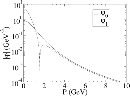
Figure 1: Ground state and first radially excited states as a function of ${\sf P}=\sqrt{2(\kappa^{2}+q^{2})}$ for $b=640$ MeV and $a=9/4$.

Table 1: Values of the parameters of the ground state wave function used for the three different forms of kinematics. The corresponding matter radii $r_{0}$ are listed in the last column.

	$m_{q}$ (MeV)	$b$ (MeV)	$a$	$r_{0}$ (fm)
point form	350	640	9/4	0.19
front form	250	500	4	0.55
instant form	140	600	6	0.63

III.2 Quark currents

For each form of kinematics the dynamics generates the current-density operator from a kinematic current, which is specified by the expression:

$$\langle{\vec{v}_{f},\vec{v}_{2}^{\prime},\vec{v}_{3}^{\prime}}|I^{\mu}(0)|{\vec{v}_{3},\vec{v}_{2},\vec{v}_{a}}\rangle=\delta^{(3)}(v_{3}^{\prime}-v_{3})\delta^{(3)}(v_{2}^{\prime}-v_{2})\left({\textstyle{1\over 6}}+{\textstyle{1\over 2}}\tau_{3}^{(1)}\right)\bar{u}(\vec{v}_{1}\,^{\prime})\gamma^{(1)\mu}u(\vec{v}_{1})\,,$$ (60)

in the case of Lorentz kinematics, and:

$$\langle{P^{+},P_{\perp f},{\bf p}_{2}^{\prime},{\bf p_{3}}^{\prime}}|I^{+}(x^{-},x_{\perp})|{{\bf p}_{3},{\bf p_{2}},P_{\perp a},P^{+}}\rangle$$ (61)

$$=\delta^{(3)}(p_{3}^{\prime}-p_{3})\delta^{(3)}(p_{2}^{\prime}-p_{2})({\textstyle{1\over 6}}+{\textstyle{1\over 2}}\tau_{3}^{(1)})\bar{u}({\bf p_{1}^{\prime}})\gamma^{(1)+}u({\bf p_{1}})e^{\imath(P_{\perp f}-P_{\perp a})\cdot x_{\perp}}\,,$$ (62)

for light-front kinematics and finally by:

$$\langle{{\textstyle{1\over 2}}\vec{Q},\vec{p}^{\prime}_{2},\vec{p}_{3}^{\prime}}|I^{\mu}(\vec{x})|{\vec{p}_{3},\vec{p}_{2},-{\textstyle{1\over 2}}\vec{Q}}\rangle=\delta^{(3)}(p_{3}^{\prime}-p_{3})\delta^{(3)}(p_{2}^{\prime}-p_{2})({\textstyle{1\over 6}}+{\textstyle{1\over 2}}\tau_{3}^{(1)})$$

$$\bar{u}(\vec{p}_{1}\,^{\prime})\gamma^{(1)\mu}u(\vec{p}_{1})e^{\imath(\vec{Q}\cdot\vec{x})}\,,$$ (63)

for instant kinematics. In each case only covariance under the kinematic subgroup is required.

For the corresponding expression for the axial vector current the matrix is obtained by the replacement:

$$\left({\textstyle{1\over 6}}+{\textstyle{1\over 2}}\tau_{3}^{(1)}\right)\gamma^{(1)\mu}\;\to\;\left(\gamma^{(1)}_{\mu}+g_{P}{(p_{1}^{\prime}-p_{1})^{\mu}\over 2m}\right)\gamma^{(1)}_{5}{\textstyle{1\over 2}}\tau^{(1)}_{3}\,.$$ (64)

The value for the pseudoscalar coupling constant of the “partially conserved” axial current is then

$$g_{P}={4m^{2}\over Q^{2}+m_{\pi}^{2}}\,.$$ (65)

III.3 Velocity representations of the quark structure

With Lorentz kinematics quark momenta $p_{i}:=mv_{i}$ are defined by the boost relations:

$$p_{i}:=B(v)\{0,\vec{k}_{i}\}+\omega_{i}v_{K}\;\,,\qquad\omega_{i}:=\sqrt{|\vec{k}_{i}|^{2}+m^{2}}\;,\qquad v_{K}^{2}=-1\;\,.$$ (66)

The Lorentz covariance of the quark velocity operators follows from the Lorentz covariance (7) and (47) of the operator $v$ and the momenta $\vec{k}_{i}$. The quark velocities do not commute with any component of the momentum $P={\cal M}v$, and the sum of the quark momenta does not equal the total momentum for any component.

Null-plane kinematics depends on a null vector $n$ or the “frame” in which
$n=\{-1,0,0,1\}$. The quark momenta $p_{i}$ defined by

$$p_{i}^{+}=\xi_{i}P^{+}\;,\qquad p_{i\perp}:=k_{i\perp}+\xi_{i}P_{\perp}\;\qquad p_{i}^{-}:={m^{2}+p_{i\perp}^{2}\over p_{i}^{+}}\qquad\mbox{with}\qquad\xi_{i}:={k_{iz}+\omega_{i}\over\sum_{i}\omega_{i}}\,,$$ (67)

are covariant only under the subgroup which leaves the null-plane $n\cdot x=0$ invariant.

With instant form kinematics the kinematic subgroup does not include any boosts. The kinematic symmetry of the quark momenta merely requires covariance under rotations and $\sum_{i}\vec{p}_{i}=\vec{P}$. That much allows considerable freedom in the relation of the quark momenta $\vec{p}_{i}$ to the internal momenta. In Ref. coe98 the momenta $\vec{p}_{i}$ were defined as functions of the boosted Jacobi momenta $B_{c}(v)\{0,\vec{\kappa}\}$ , $B_{c}(v)\{0,\vec{q}\}$ and the total momentum $\vec{P}$. That definition had the virtue of formal simplicity. Here the velocities $\vec{p}_{i}/m$ are taken to be free-quark velocities, which implies

$$p_{i}=\omega_{i}v_{K}+B_{c}(v_{K})\{0,\vec{k}_{i}\}\ = \{v_{Kz}k_{iz}+\omega_{i}v_{K}^{0},k_{ix},k_{iy},v_{K}^{0}k_{iz}+\omega_{i}v_{Kz}\}\ ,$$ (68)

$$\vec{k}_{i} = \{p_{ix},p_{iy},v_{K}^{0}p_{iz}-E_{i}v_{Kz}\}\ \,,$$ (69)

with $\vec{v}_{K}:=\vec{P}/\sum_{i}\omega_{i}$. Canonical boosts are used because then the Wigner rotations of rotations are identical to the rotations.

The quark momenta so defined by either Eq. (67) or (69) are covariant under the kinematic subgroup, that is

$$U^{\dagger}(\Lambda)p_{i}U(\Lambda)=\Lambda p_{i}\,,$$ (70)

with $\Lambda$ restricted to the kinematic subgroup.

For the three forms of kinematics changes in the representation of the baryon states:

$$\{\vec{\kappa},\vec{q},\vec{v}\} \to \{\vec{p}_{2},\vec{p}_{3},\vec{v}\}\qquad\mbox{with}\qquad\vec{p}_{1}=\vec{p}_{1}(\vec{p}_{2},\vec{p}_{3},\vec{v})\,,$$

$$\{\vec{\kappa},\vec{q},{\bf P}\} \to \{{\bf p_{2}},{\bf p_{3}},{\bf P}\}\qquad\mbox{with}\qquad{\bf p_{1}}={\bf P}-{\bf p_{2}}-{\bf p_{3}}\,,$$

$$\{\vec{\kappa},\vec{q},\vec{P}\} \to \{\vec{p}_{2},\vec{p}_{3},\vec{P}\}\qquad\mbox{with}\qquad\vec{p}_{1}=\vec{P}-\vec{p}_{2}-\vec{p}_{3}\,,$$ (71)

together with the corresponding spin to spinor transformations coe92 ,

$$u_{c}(v_{i}) = {\vec{\alpha}\cdot\vec{v}_{i}+\beta+v_{i}^{0}\over\sqrt{2v_{i}^{0}(1+v_{i}^{0})}}{1+\beta\over 2}\,,$$ (72)

$$u_{f}(\bf p_{i}) = {\vec{\alpha}_{\perp}\cdot\vec{p}_{\perp}+\beta m+p^{+}\over\sqrt{2mp^{+}}}{1+\alpha_{3}\over 2}{1+\beta\over 2}\,,$$ (73)

$$u_{c}(\vec{p}_{i}) = {\vec{\alpha}\cdot\vec{p}_{i}+m\beta+E_{i}\over\sqrt{2E_{i}(m+E_{i})}}{1+\beta\over 2}\;,\qquad E_{i}:=\sqrt{m^{2}+|\vec{p}_{i}|^{2}}\,,$$ (74)

provide kinematically covariant representations of the baryon states, which are convenient for the construction of conserved current density operators which satisfy Poincaré covariance.

In each case the wave function must be multiplied by the square root of the appropriate Jacobian. For Lorentz kinematics this is

$$J(\vec{v};\vec{p}_{2},\vec{p}_{3}):=\left({\partial(\vec{\kappa},\vec{q})\over\partial(\vec{p}_{2},\vec{p}_{3})}\right)_{\vec{v}}={\sqrt{27}\omega_{2}\omega_{3}\over E_{2}E_{3}}={\sqrt{27}(E_{2}v^{0}-p_{2z}v_{z})(E_{3}v^{0}-p_{3z}v_{z})\over E_{2}E_{3}}\,.$$ (75)

With null plane kinematics the Jacobian is

$$J(\bf P;\bf p_{2},\bf p_{3}) := \left({\partial(\vec{\kappa},\vec{q})\over\partial({\bf p}_{2},{\bf p}_{3})}\right)_{\bf P}={\partial(\vec{\kappa},\vec{q})\over\partial(\xi_{2},k_{2\perp},\xi_{3},k_{3\perp})}\,\left({\partial(\xi_{2},k_{2\perp},\xi_{3},k_{3\perp})\over\partial({\bf p_{2}},{\bf p_{3}})}\right)_{\bf P}$$ (76)

$$= {\sqrt{27}\omega_{1}\omega_{2}\omega\,_{3}(P^{+})\over p_{1}^{+}p_{2}^{+}p_{3}^{+}(\omega_{1}+\omega_{2}+\omega_{3})}\,,$$ (78)

with

$$\omega_{i}={\textstyle{1\over 2}}\left(\xi_{i}M_{0}+{m^{2}+k_{i\perp}^{2}\over\xi_{i}M_{0}}\right)\;,\qquad M_{0}^{2}=\sum_{i}{m^{2}+k_{i\perp}^{2}\over\xi_{i}}=\left(\sum_{i}\omega_{i}\right)^{2}\,.$$ (79)

With instant kinematics the definition (69) implies the Jacobian:

$$J(\vec{P},\vec{p}_{2},\vec{p}_{3}) := \left({\partial\vec{\kappa},\vec{q})\over\partial(\vec{p}_{2},\vec{p}_{3})}\right)_{\vec{P}}=\sqrt{27}{\partial(\vec{k}_{2},\vec{k}_{3},\vec{v})\over\partial(\vec{p}_{2},\vec{p}_{3},\vec{v})}\;{\partial(\vec{k}_{2},\vec{k}_{3},\vec{P})\over\partial(\vec{k}_{2},\vec{k}_{3},\vec{v})}\;{\partial(\vec{p}_{2},\vec{p}_{3},\vec{v})\over\partial(\vec{p}_{2},\vec{p}_{3},\vec{P})}$$ (80)

$$= {\sqrt{27}\omega_{2}\omega_{3}\over E_{2}E_{3}}\left(1-v_{z}{k_{1z}\over E_{1}}\right)$$ (82)

where

$$P_{x}=P_{y}=0\;,\qquad M_{0}^{2}=(\sum_{i}E_{i})^{2}-|\vec{P}|^{2}\;,\qquad\vec{v}:={\vec{P}\over M_{0}}\,.$$ (83)

With canonical boosts the spin variables must be transformed by the required momentum dependent rotation matrices

$$D^{\textstyle{1\over 2}}_{\lambda_{i},\sigma_{i}}\left(R_{W}[B(v_{K}),k_{i}]\right)\qquad\mbox{with}\qquad R_{W}[B(v_{K}),k_{i}]:=B^{-1}(p_{i})B(v_{K})B(k_{i})\;.$$ (84)

With canonical boosts explicit representations of these Wigner rotations are,

$$D^{1/2}\Bigl{(}{\cal R}_{W}[B(v_{K}),k_{i}]\Bigr{)}=\cos{\theta_{i}\over 2}-\imath\sin{\theta_{i}\over 2}\,{(\vec{p}_{i}\times\vec{\sigma}_{i})_{z}\over|p_{i\perp}|}\;,\qquad i=1,2,3\,,$$ (85)

where the angles $\theta_{i}$ are defined by

$$\sin{\theta_{i}\over 2}=-{v_{Kz}|p_{i\perp}|\over\sqrt{2(1+v_{K}^{0})(m+E_{i})(m+\omega_{i})}}\,.$$ (86)

.

With null-plane kinematics the corresponding required spin rotations are Melosh rotations, which are represented by coe92

$$D^{\textstyle{1\over 2}}[{\cal R}_{M}(\vec{k}_{i})]={m+\xi_{i}M_{0}-\imath\vec{\sigma}\cdot(\vec{n}\times\vec{k}_{i\perp})\over[(m+\xi_{i}M_{0})^{2}+\vec{k}_{i\perp}^{2}]^{1/2}}\,.$$ (87)

IV Nucleon form factors

IV.1 Canonical spin representations

The matrix elements (II.1) may be evaluated with the antisymmetric nucleon wave function (54) and the quark current (60) multiplied by 3 (the number of constituent quarks). Evaluation of the sum over spin and isospin indices leads to the explicit expressions of the form factors

$$G_{E}(\eta) = \int d^{3}p_{2}d^{3}p_{3}\,\varphi\left({{\kappa^{\prime}}^{2}+q^{{}^{\prime}2}\over 2b^{2}}\right)\varphi\left({\kappa^{2}+q^{2}\over 2b^{2}}\right)\sqrt{{\cal J}_{fa}(\vec{p}_{2},\vec{p}_{3})}C_{23}(\eta,\vec{p}_{2},\vec{p}_{3}){\cal S}_{e}(\eta,\vec{p}_{2},\vec{p}_{3}),$$ (88)

$$G_{M}(\eta) = \int d^{3}p_{2}d^{3}p_{3}\varphi\left({{\kappa^{\prime}}^{2}+q^{{}^{\prime}2}\over 2b^{2}}\right)\varphi\left({\kappa^{2}+q^{2}\over 2b^{2}}\right)\sqrt{{\cal J}_{fa}(\vec{p}_{2},\vec{p}_{3})}C_{23}(\eta,\vec{p}_{2},\vec{p}_{3}){\cal S}_{m}(\eta,\vec{p}_{2},\vec{p}_{3})\;.$$ (91)

The Jacobian factor ${\cal J}_{fa}$,

$${\cal J}_{fa}:=J(v_{f},\vec{p}_{2},\vec{p}_{3})J(v_{a},\vec{p}_{2},\vec{p}_{3})\,,$$ (93)

is defined by Eq. (75) or (LABEL:instjac) for Lorentz or instant kinematics respectively.

The coefficient $C_{23}(\eta,\vec{p}_{2},\vec{p}_{3})$ is determined by the spectator Wigner rotations:

$$C_{23}(\eta,\vec{p}_{2},\vec{p}_{3}) = {1\over 2}\sum_{\sigma^{\prime},\sigma}\left[\sum_{\sigma^{\prime\prime}}{{\cal D}^{1/2}_{\sigma^{\prime}\sigma^{\prime\prime}}}^{\dagger}\left({\cal R}_{W}[B(v_{Kf}),k^{\prime}_{2}]\right){\cal D}^{1/2}_{\sigma^{\prime\prime},\sigma}\left({\cal R}_{W}[B(v_{Ka}),k_{2}]\right)\right]$$ (94)

$$\times \left[\sum_{\sigma^{\prime\prime}}{{\cal D}^{1/2}_{-\sigma^{\prime}\sigma^{\prime\prime}}}^{\dagger}\left({\cal R}_{W}[B(v_{Kf}),k^{\prime}_{3}]\right)D^{1/2}_{\sigma^{\prime\prime},-\sigma}\left({\cal R}_{W}[B(v_{Ka}),k_{3}]\right)\right]\;.$$ (96)

The velocities $\vec{v}_{Ka}$, $\vec{v}_{Kf}$ are $\vec{v}_{a}$, $\vec{v}_{f}$ with Lorentz kinematics and ${\textstyle{1\over 2}}\vec{Q}/{\cal M}_{0}^{\prime}$, $-{\textstyle{1\over 2}}\vec{Q}/{\cal M}_{0}$ with instant kinematics.

The factors ${\cal S}_{e}$ and ${\cal S}_{m}$ arise from the Dirac spinor structure of the current and associated Wigner rotations. The explicit expressions are

$${\cal S}_{e} = \langle{{\textstyle{1\over 2}}}|{D^{\textstyle{1\over 2}}}^{\dagger}[{\cal R}_{W}(v_{Kf},k_{1}^{\prime})]\,\bar{u}_{c}(v_{1}^{\prime})\,\gamma^{0}\,u_{c}(v_{1})\,D^{\textstyle{1\over 2}}[{\cal R}_{W}(v_{Ka},k_{1})]|{{\textstyle{1\over 2}}}\rangle$$ (97)

$$= \sqrt{{(E_{1}^{\prime}+m)(E_{1}+m)(1+\eta)\over 4E_{1}^{\prime}E_{1}}}\bigg{\{}\left[1+{\vec{p}_{1}\,^{\prime}\cdot\vec{p}_{1}\over(E_{1}^{\prime}+m)(E_{1}+m)}\right]\cos\left({\theta_{1}-\theta_{1}^{\prime}\over 2}\right)$$ (101)

$$+{|p_{1\perp}|(p_{1z}^{\prime}-p_{1z})\over(E_{1}^{\prime}+m)(E_{1}+m)}\sin\left({\theta_{1}-\theta_{1}^{\prime}\over 2}\right)\bigg{\}}\;,$$

and

$${\cal S}_{m} = {1\over\sqrt{\eta}}\langle{{\textstyle{1\over 2}}}|{D^{\textstyle{1\over 2}}}^{\dagger}[{\cal R}_{W}(v_{Kf},k_{1}^{\prime})]\,\bar{u}_{c}(v_{1}^{\prime})\,\gamma_{x}\,u_{c}(v_{1})\,D^{\textstyle{1\over 2}}[{\cal R}_{W}(v_{Ka},k_{1})]\,|{-{\textstyle{1\over 2}}}\rangle$$ (102)

$$= \sqrt{{1+\eta\over 4\eta E_{1}^{\prime}(E_{1}^{\prime}+m)E_{1}(E_{1}+m)}}\bigg{\{}\Bigl{[}p_{1z}^{\prime}(E_{1}+m)-p_{1z}(E^{\prime}_{1}+m)\Bigr{]}\cos{\theta_{1}^{\prime}\over 2}\cos{\theta_{1}\over 2}$$ (104)

$$+ {1\over 2}|p_{1\perp}|(E_{1}^{\prime}+E_{1}+2m)\sin{\theta_{1}^{\prime}-\theta_{1}\over 2}+{1\over 2}|p_{1\perp}|(E_{1}-E_{1}^{\prime})\sin{\theta_{1}^{\prime}+\theta_{1}\over 2}\bigg{\}},$$ (106)

respectively. The boost dependent angles of rotation of the initial and final spins of the struck constituent are defined in Eq.(86).

In Appendix C and D the corresponding expressions for the matrix elements relevant for the calculation of the axial and $N\to\Delta$ transition form factors are given.

IV.2 Light-front spin representations

The form factors of the proton, $\tau={\textstyle{1\over 2}}$, and the neutron, $\tau=-{\textstyle{1\over 2}}$,

$$F_{1,\tau}(Q^{2}):=\langle{{\textstyle{1\over 2}},\tau}|I^{+}(0)|{\tau,{\textstyle{1\over 2}}}\rangle\,,\qquad F_{2,\tau}(Q^{2}):={1\over\sqrt{\eta}}\langle{-{\textstyle{1\over 2}},\tau}|I^{+}(0)|{\tau,{\textstyle{1\over 2}}}\rangle,$$ (107)

can be written in a compact form as,

$$F_{\alpha,\tau}(Q^{2}) = \int_{0}^{1}d\xi_{1}\,d\xi_{2}\,d\xi_{3}\,{\delta(\xi_{1}+\xi_{2}+\xi_{3}-1)\over\xi_{1}\xi_{2}\xi_{3}}\,$$ (108)

$$\int d\vec{k}_{1\perp}\,d\vec{k}_{2\perp}\,d\vec{k}_{3\perp}\,\delta(\vec{k}_{1\perp}+\vec{k}_{2\perp}+\vec{k}_{3\perp})\sqrt{{\omega_{1}\omega_{2}\omega_{3}\over M_{0}}{\omega_{1}^{\prime}\omega_{2}^{\prime}\omega_{3}^{\prime}\over M_{0}^{\prime}}}\,$$

$$\varphi^{*}(\xi_{1},\vec{k}_{1\perp}^{\prime},\xi_{2},\vec{k}_{2\perp}^{\prime},\xi_{3},\vec{k}_{3\perp}^{\prime}){\cal F}_{\alpha,\tau}(Q^{2})\varphi(\xi_{1},\vec{k}_{1\perp},\xi_{2},\vec{k}_{2\perp},\xi_{3},\vec{k}_{3\perp})\;,$$

where

$$k_{1\perp}^{\prime}=k_{1\perp}+(1-\xi_{1})Q_{\perp}\;,\qquad k_{i\perp}^{\prime}=k_{i\perp}-\xi_{1}Q_{\perp}\qquad i=2,3\;.$$ (109)

The factors ${\cal F}_{\alpha,\tau}(Q^{2})$ involve the spin-isospin amplitudes (51) and the effects of the Melosh rotations on both spectators and the quark current $I_{q1}$,

$${\cal F}_{1,\tau}(Q^{2}) = \chi_{{\textstyle{1\over 2}},\tau}^{\dagger}\,D^{1/2\dagger}({\cal R}_{M1^{\prime}})\,\,I^{+}_{q_{1}}\,D^{1/2}({\cal R}_{M1})\;$$

$$\times D^{1/2\dagger}({\cal R}_{M2^{\prime}})D^{1/2}({\cal R}_{M2})D^{1/2\dagger}({\cal R}_{M3^{\prime}})D^{1/2}({\cal R}_{M3})\,\chi_{-{\textstyle{1\over 2}},\tau}\,,$$

$${\cal F}_{2,\tau}(Q^{2}) = {1\over\sqrt{\eta}}\chi_{-{\textstyle{1\over 2}},\tau}^{\dagger}\,D^{1/2\dagger}({\cal R}_{M1^{\prime}})\,\,I^{+}_{q_{1}}\,D^{1/2}({\cal R}_{M1})\;$$ (110)

$$\times D^{1/2\dagger}({\cal R}_{M2^{\prime}})D^{1/2}({\cal R}_{M2})D^{1/2\dagger}({\cal R}_{M3^{\prime}})D^{1/2}({\cal R}_{M3})\,\chi_{{\textstyle{1\over 2}},\tau}\,.$$

The representations of the Melosh rotations are defined in Eq. (87).

In the explicit evaluation of the integrals the choice $p_{2\perp}=p_{2x}$ is made without loss of generality. This leads to the following expressions for ${\cal F}_{i}(Q^{2})$ :

$${\cal F}_{1p} = {1\over D_{1}D_{2}D_{3}}f_{1}[f_{2}f_{3}+V_{2y}V_{3y}]\,,$$

$${\cal F}_{2p} = {2m_{p}\over Q}{1\over D_{1}D_{2}D_{3}}(-V_{1y})[f_{2}f_{3}+V_{2y}V_{3y}]\,,$$

$${\cal F}_{1n} = {-1\over 3}{1\over D_{1}D_{2}D_{3}}[2f_{1}V_{2y}V_{3y}-f_{2}V_{1z}V_{3z}-f_{2}V_{1x}V_{3x}-f_{2}V_{1y}V_{3y}-f_{3}V_{1y}V_{2y}]\,,$$

$${\cal F}_{2n} = {2\over 3}{m_{p}\over Q}{1\over D_{1}D_{2}D_{3}}[2V_{1y}f_{2}f_{3}-V_{1x}V_{2y}V_{3x}-f_{1}f_{2}V_{3y}-f_{1}f_{3}V_{2y}-V_{1z}V_{3z}V_{2y}]\,.$$ (111)

Here the following notation has been employed:

$$a_{i} = m+\xi_{i}M_{0}\,,\qquad a_{i}^{\prime}=m+\xi_{i}M_{0}^{\prime}\,,\qquad\vec{n}=(0,0,1)\,,$$

$$D_{i} = \sqrt{{a^{\prime}}_{k}^{2}+\vec{k^{\prime}}_{i\perp}^{2}}\;\sqrt{a_{k}^{2}+\vec{k}_{i\perp}^{2}}\,,$$

$$f_{i} = a^{\prime}_{i}a_{i}+\vec{k^{\prime}}_{i\perp}\cdot\vec{k}_{i\perp}\,,$$

$$\vec{V}_{k} = -a_{k}(\vec{n}\times\vec{k^{\prime}}_{i\perp})+a^{\prime}_{k}(\vec{n}\times\vec{k}_{i\perp})+(\vec{n}\times\vec{k^{\prime}}_{i\perp})\times(\vec{n}\times\vec{k}_{i\perp})\,.$$ (112)

In Appendix E the corresponding expressions for the matrix elements relevant for the computation of the axial form factors are given.

V Numerical results

V.1 Nucleons

V.1.1 Finite values of the constituent mass

In order to explore qualitative differences of the three forms of kinematics nucleon form factors were calculated with the mass and current operators specified in Sec. III with the parameter values listed in Table 1.

The calculated form factors are shown in Figs. 2, 3, 5 and 6 along with data taken from the compilation gep . In Table 2 the corresponding values of $G_{Mp}(0)$, $G_{Mn}(0)$, $G_{A}$(0) together with the proton charge radii are listed. The rms radius $r_{0}$ of the wave function is always smaller than the charge radius with the largest value for instant kinematics and the smallest for Lorentz kinematics.

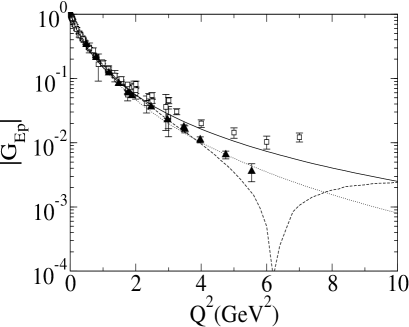
Figure 2: Electric form factor of the proton. Solid, dotted and dashed lines correspond to the instant, point and front forms respectively. Squares are from the compilation of Ref. gep while black triangles are obtained from the recent JLAB data of Refs. jones using
$G_{Ep}=(\mu_{p}G_{Ep}/G_{Mp})/(1+Q^{2}/0.71)^{2}$.

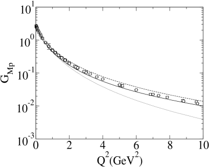
Figure 3: Magnetic form factor of the proton. Solid, dotted and dashed lines correspond to the instant, point and front forms respectively. The experimental data are from the compilation of Ref. gep .

Table 2: Values of the form factors at $Q^{2}\rightarrow 0$ together with the proton charge radius.

	Instant	Point	Front	EXP
$G_{Mp}(0)$	2.7	2.5	2.8	2.793 PDG
$G_{Mn}(0)$	$-$1.8	$-$1.6	$-$1.7	$-$1.913 PDG
$G_{A}(0)$	1.1	1.1	1.2	1.2670 PDG
$r_{cp}$(fm)	0.89	0.84	0.85	0.87 PDG

The results reveal that it is possible to reach agreement with the empirical data for all these form factors. The electric form factor of the proton is found to be more sensitive to the form of kinematics than the magnetic form factors. That may be related to the implementation of current conservation, which involves the form of dynamics.

The instant form result for $G_{Ep}$ in Fig. 2 follows the empirical values obtained by a Rosenbluth separation up to 6 GeV². The point form calculation, with a very compact wave function, follows the data that have been obtained by means of polarization transfer somewhat more closely. The front form calculation of the form factors $F_{1}$ and $F_{2}$ produces cancellations of $F_{1}$ and $\eta F_{2}$ at about $6$ GeV² Miller ; brodsky . Such behavior is in fact suggested by the recent experimental data for the quotient $\mu_{p}G_{Ep}/G_{Mp}$ jones . In Fig. 4 this ratio is shown as calculated with the three forms of kinematics. This figure emphasizes the differences between the three forms of kinematics as well as the discrepancies in the form factors of the proton at medium energies. This discrepancy between the recent TJNAF data, measured using the polarization transfer technique, and the previous data, obtained through the Rosenbluth separation arrington , could be partly due to two photon exchanges as recently explored in Ref. blunden . There is therefore a qualitative difference between models based on canonical-spin representations of the currents (instant and Lorentz kinematics) and models based on null-plane-spin representations of the currents (front-form kinematics).

Similar results for the elastic form factors have been described in the literature making use of point boffi ; coe03 and front ck95 forms of kinematics on the basis of different dynamical models.

The calculated values of the magnetic form factors shown in Figs. 3 and 5 are in qualitative agreement with each other and the data. The calculated magnetic moments show significant differences. With instant form kinematics reasonable agreement with the empirical values of the nucleon magnetic moments requires a very small quark mass of 140 MeV. With larger quark mass values the magnitude of the calculated magnetic moments is too small. This feature also appears in the non-relativistic quark model with “relativistic corrections” dannb . The missing strength is in that model attributed to exchange current contributions.

The magnetic moment values that are obtained in point form kinematics are about 10 % too small. This feature was already noted in Ref. boffi . In this case the calculated values of the magnetic moments are fairly insensitive to the quark mass value.

The magnetic moment of the proton as calculated in front form kinematics with a wave function of intermediate range also falls within 1 % of the empirical value. In front form kinematics the calculated neutron magnetic moment falls some 12 % below the corresponding empirical value.

The calculated value of the axial vector coupling constant, $G_{A}(0)$, is closest to the empirical value (within 6 %) when front form kinematics is used. In instant and point form kinematics the calculated value is about 14 % smaller than the empirical value. These values differ significantly from the static quark model value $5/3$, which is too large by 31 %.

The calculated values of the axial form factor are close to the empirical values ga in all forms of kinematics as shown in Fig 6. The pseudoscalar form factor follows the empirical values, except at very small values of momentum transfer, where only the front-form one actually goes through the muon point.

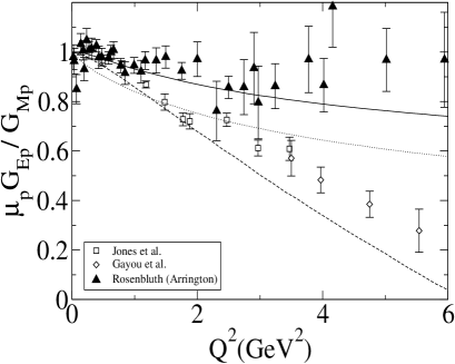
Figure 4: Quotient $\mu_{p}G_{Ep}/G_{Mp}$ compared to the recent experimental data measured in TJNAF, Refs. jones ; arrington . Solid, dotted and dashed lines correspond to the instant, point and front forms respectively.

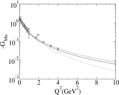
Figure 5: Magnetic form factors of the neutron. Solid, dotted and dashed lines correspond to the instant, point and front forms respectively. The experimental data are from the compilation of Ref. gep .

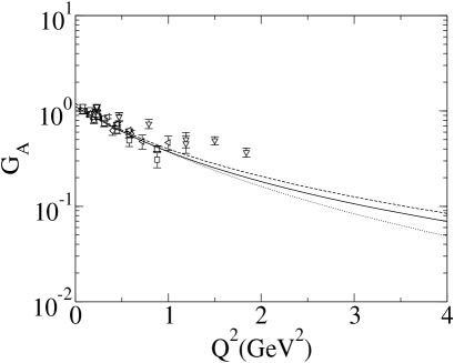
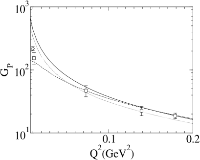
Figure 6: Axial and induced pseudoscalar form factors of the nucleon. Solid, dotted and dashed lines correspond to the instant, point and front forms respectively. The experimental data are from Refs. ga ; gp .

V.1.2 The electric form factor of the neutron

Without the momentum dependent spin rotations (85) or (87) the symmetric spin-isospin amplitude (51) would imply a vanishing electric form factor of the neutron. Because of Wigner rotations or Melosh rotations of the constituent spins the electric form factor of the neutron does not vanish. This is shown in Fig. 7a. The magnitude is however negligible with instant and point form kinematics and too small with front form kinematics in agreement with the results of Refs. Chung ; Simula .

In Ref. boffi , using point form kinematics, it was noted that a small admixture of a mixed symmetry $S-$state in the ground state may produce a satisfactory form factor. The effects of a $2\%$ admixture of a mixed symmetry $S-$state wave function are also shown in Fig. 7b for all three forms of kinematics. The results are in good agreement with the empirical data. The agreement is not quite as good with a 1% admixture of the mixed symmetry $S-$state and would deteriorate with a larger admixture.

The mixed symmetry $S-$state is represented by appropriate combination of mixed symmetry spin-isospin wave functions with two radial wave functions of mixed symmetry of the form

$$\varphi_{s}(\vec{\kappa},\vec{q})={\cal N}_{s}{\kappa^{2}-q^{2}\over\kappa^{2}+q^{2}}\varphi_{0}(\kappa,q)\,,\quad\varphi_{a}(\vec{\kappa},\vec{q})={\cal N}_{a}{\vec{\kappa}\cdot\vec{q}\over\kappa^{2}+q^{2}}\varphi_{0}(\kappa,q)\,.$$ (113)

where $\varphi_{0}(\vec{\kappa},q)$ is the symmetric $S-$state wave function (54). The explicit construction is given in Appendix B.

The effect of the introduction of the mixed symmetry $S-$state component on the other nucleon form factors is small. This is illustrated in Fig.8, where the modification of the calculated front form electric and magnetic proton form factors by the mixed symmetry $S-$state is shown. The values of the slope $(dG_{en}/dQ^{2})_{Q^{2}=0}$ that are obtained are 0.60 GeV^-2, 0.56 GeV^-2 and 0.39 GeV^-2 for instant, point and front form respectively, while the experimental value is 0.511$\pm$0.008 GeV^-2 genexp .

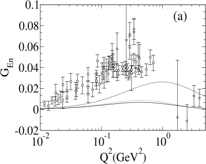
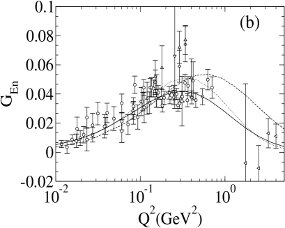
Figure 7: Electric form factor of the neutron. Solid, dotted and dashed lines correspond to the instant, point and front forms respectively. (a) No mixed symmetry $S-$state is included. (b) Some percentage of mixed symmetry $S-$state is included in the neutron wave function as described in the text. Experimental data are from Refs. gep .

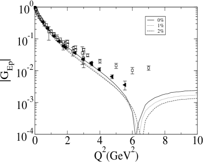
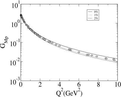
Figure 8: Electric (left) and magnetic (right) form factors of the proton calculated with front-form kinematics with some mixed symmetry $S-$state component as explained in the text. Solid, dotted and dashed lines correspond to $0\%$, $1\%$ and $2\%$ of mixed symmetry $S-$state. Squares are from the compilation of Ref. gep while black triangles are obtained from the recent JLAB data of Refs. jones using $G_{Ep}=(\mu_{p}G_{Ep}/G_{Mp})/(1+Q^{2}/0.71)^{2}$.

V.1.3 The zero quark mass limit

It has been noted coe03 that in the case of point form kinematics and spectator currents the form factors were insensitive to unitary scale transformations of the wave functions when the extent of the wave function was small compared to the scale defined by the quark mass, $<r^{2}>\ll 1/m_{q}^{2}$. This is equivalent to $b^{2}\gg m_{q}^{2}$. In the “point” limit $m_{q}^{2}/b^{2}=0$ the calculated form factors are invariant under unitary scale transformations. This opens the possibility for quark model phenomenology with a very small constituent mass.

For the class of quark models considered here, where the representation of the baryon mass operator is independent of the quark mass, a zero-quark-mass limit of the form factors exists for all three forms of kinematics. The spinor representations of the quark currents and the boost transformations to spin representations are also independent of the quark mass. Only the Jacobians and the Wigner or Melosh rotations depend on the quark mass.

Zero-quark-mass values of the magnetic moments and the axial coupling constant are listed in Table 3. In Figs. 9 and 10 the zero-mass limits of nucleon magnetic and axial form factors are compared to the finite-mass values. The magnetic moments of both the protons and the neutrons do not show large changes with vanishing mass in the case of instant form kinematics. The results for the nucleon magnetic form factors, see Fig. 9, in the zero mass limit show that the form factors are insensitive to the quark mass only with Lorentz kinematics.

Table 3: Values of the form factors at $Q^{2}\rightarrow 0$ for zero constituent mass. 

	Instant	Point	Front	EXP
$G_{Mp}(0)$	2.6	2.	3.2	2.793 PDG
$G_{Mn}(0)$	$-$1.7	$-$1.3	$-$2.0	$-$1.913 PDG
$G_{A}(0)$	0.6	0.6	0.0	1.2670 PDG

Fig. 11 shows magnetic form factors computed with zero quark mass and wave functions with different rms radii obtained varying the exponent $a$ with fixed $b$. Thus both the range and the shape of the wave function are changed. The point form results show the expected scale independence and indicate that the change in shape is relatively unimportant. With instant and front-form kinematics. Fig. 11 shows the expected drastic changes in the $Q^{2}$ dependence In particular, instant form calculations do not reproduce the experimental behavior at high-$Q^{2}$ for any of the exponents, while front form ones do give the correct behavior for the appropriate value of $a$.

The zero mass limit does not yield satisfactory values for the axial coupling constant and the axial form factor, as seen in Table 3 and in Fig.10. These results suggest that realistic axial current phenomenology in the constituent quark model demands that the constituent mass at least be of the order of 200 MeV. Overall, the zero-quark-mass limit is not a good candidate for quark-model phenomenology if both axial and electromagnetic properties are to be understood simultaneously.

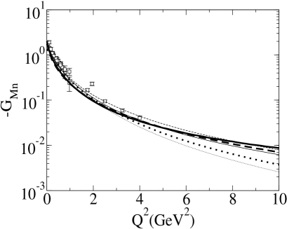
Figure 9: Magnetic form factor of the proton(left), of the neutron(right). Solid, dotted and dashed lines correspond to the instant, point and front forms respectively. Thick lines correspond to the zero quark mass case. Experimental data are from Refs. gep .

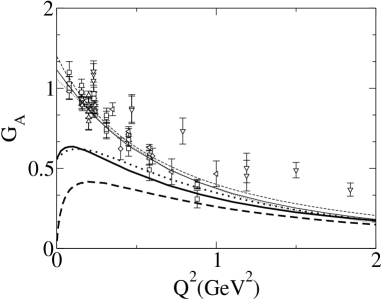
Figure 10: Axial form factor. Solid, dotted and dashed lines correspond to the instant, point and front forms respectively. Thick lines correspond to the zero quark mass case. Experimental data are from Refs. ga .

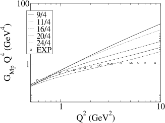
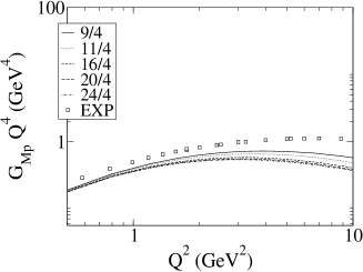
Figure 11: Magnetic form factor of the proton for $m_{q}=0$ in instant(above-left), point(above-right) and front(below) forms respectively. The different lines correspond to different values of the exponent $a$ in Eq. (54). Experimental data are from Refs. gep .

V.2 The $\Delta(1232)\rightarrow N$ transition form factors

The magnetic transition form factor $G_{M\Delta}$ that is associated with the $\Delta(1232)-N$ transition as calculated with the wave function (54) and the parameter values in Table 1 in the three forms of kinematics is shown in Fig. 12. The corresponding values for the transition magnetic moments are listed in Table 4.

In the case of instant form kinematics the impulse approximation describes the empirical form factor and the transition magnetic moment well. This is a notable improvement compared to non-relativistic quark models. The magnetic moment is too small by about 30 % in both point and front kinematics.

Table 4: The $\Delta(1232)-N$ transition magnetic moment in the different forms of kinematics with finite and zero constituent mass. 

	Instant	Point	Front	EXP
$G_{M\Delta}(0)$ $m\neq 0$	2.8	2.0	2.1	3.1
$G_{M\Delta}(0)$ $m=0$	3.0	1.7	2.5	3.1

In Table 4 the transition magnetic moments are also listed as obtained in the zero quark mass case. The corresponding form factors are plotted in Fig. 13. These results are fairly similar to those obtained with finite values of the constituent mass.

V.3 The $N(1440)\rightarrow N$ form factors

In Fig. 14 we show the calculated helicity amplitude $A_{1/2}$, defined as:

$$A_{1/2}=\sqrt{{4\pi\alpha\over 2E_{\gamma}}}\sqrt{\eta}G_{M}\qquad E_{\gamma}:={M^{*2}-M^{2}\over 2M^{*}}\quad\alpha\sim 1/137\,,$$ (114)

for the $N(1440)-N$ transition as obtained with the wave function models (54) and (58) in all forms of kinematics with the parameter values in Table 1. It is, of course, questionable whether a treatment of the $N(1440)$ as a stable 3-quark bound state is realistic. The extant data of this helicity amplitude shown in Fig. 14 exproper ; CLAS are manifestly inadequate. The calculated transition form factors do in this case depend significantly on the form of kinematics.

In Fig 15 the helicity amplitude obtained with zero quark mass is shown. These results are qualitatively similar to those that are obtained with finite values of the constituent mass above.

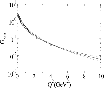
Figure 12: Magnetic $\Delta\rightarrow N$ transition form factor. Solid, dotted and dashed lines correspond to the instant, point and front forms respectively. Experimental data are from Refs. gnd .

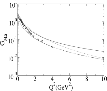
Figure 13: Magnetic $\Delta\rightarrow N$ transition form factor in the zero quark mass case. Solid, dotted and dashed lines correspond to the instant, point and front forms respectively. Experimental data are from Refs. gnd .

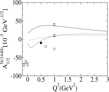
Figure 14: Helicity amplitude for $N^{*}(1440)$ electroexcitation. Solid, dotted and dashed lines correspond to the instant, point and front forms respectively. The experimental data are from Refs. exproper . The full solid point also corresponds to a preliminary analysis from CLAS  CLAS .

Figure 15: Helicity amplitude for $N^{*}(1440)$ electroexcitation in the zero quark mass case. Solid, dotted and dashed lines correspond to the instant, point and front forms respectively. The experimental data are from Refs. exproper . The full solid point also corresponds to a preliminary analysis from CLAS  CLAS .

VI Conclusions

The present comparative study of how baryon form factors calculated with free-quark currents depend on the choice of the kinematic subgroup revealed a number of features, which might be of phenomenological utility in description of the baryons by constituent-quark models. This exploration is based on mass operators of confined quark, which are parameterized by a confinement scale, and which implement basic symmetries without free-quark features or dependence on quark masses. Poincaré covariant current density operators are generated by the dynamics from free-quark current densities covariant under different kinematic subgroups

The interpretation of baryon wave functions of constituent-quark models as a description of a physical structure that is observed by electro-weak processes depends on the choice of a form of kinematics. To assess the effectiveness of a choice of kinematics it is important to consider the full range of elastic and inelastic transitions at low and medium energies. Examination of a broad range of features with a crude model structure revealed no drastic failure that would rule out any of the forms of kinematics considered. For most form factors permutation symmetric $S-$wave functions were adequate. The electric form factor of the neutron required a small mixed-symmetry admixture. The baryon wave functions used for this exploration are independent of the quark mass and dependent on a range parameter and a shape parameter. Significantly different values of these parameters are required for adequate wave functions with different forms of kinematics. A quantitative phenomenology for all available form factor data would require different refinements with different forms of kinematics.

The calculated form factors are functions of kinematic quantities, which differ with form of kinematics and the baryon masses. Since at least one component of the four-momentum is dynamic, current conservation will always imply some dependence on the baryon masses.

The features emphasized by instant form kinematics are closest to those of non-relativistic quark models with a physical interpretation of the wave function that emphasizes covariance under 3-dimensional rotations and translations. Lorentz boosts are not in the kinematic subgroup. There is no kinematic Lorentz symmetry of quark velocities. The kinematic variable of the form factors is $\vec{Q}^{2}$ which equals the four-momentum transfer only for elastic transitions.

With light-front kinematics both relevant Lorentz boosts and translations are kinematic. The corresponding subgroup is Galilean symmetry in $1+2$ dimensions with $p_{i}^{+}$ in the role of the masses. In that case rotations about the direction of the momentum transfer are not kinematic. In this the kinematic parameter of the form factors is the four-momentum transfer $Q^{2}$

With point-form kinematics there are no kinematic translations and there is no kinematic interpretation of the wave function as a representation of spatial structure. The kinematic parameter of the form factors is the invariant velocity transfer $\eta$.

Appendix A Invariant form factors for $N\to\Delta$ transition

The best way to relate calculations made in the three forms of kinematics to the standard invariant form factors is through the following set of invariant form factors, similar to those used in Ref. Scad ,

$$\Gamma^{\mu}_{\nu}(P,Q)=\sum_{i}^{3}{\cal K}_{\nu}^{i,\mu}(P,Q)G_{i}(Q^{2})\,,$$ (115)

with,

$${\cal K}^{1,\nu\mu}(P,Q) = {Q^{\nu}\gamma^{\mu}-(\gamma\cdot Q)g^{\nu\mu}\over\sqrt{Q^{2}}}\sqrt{M^{*}M}\gamma_{5}\,,$$

$${\cal K}^{2,\nu\mu}(P,Q) = {Q^{\nu}P^{\mu}-(P\cdot Q)g^{\nu\mu}\over\sqrt{Q^{2}}}\;\gamma_{5}\,,$$

$${\cal K}^{3,\nu\mu}(P,Q) = {Q^{\nu}Q^{\mu}-Q^{2}g^{\nu\mu}\over Q^{2}}M^{*}\;\gamma_{5}\,,$$ (116)

where $M$ and $M^{*}$ are the nucleon and resonance masses respectively. The Sachs like magnetic dipole, electric quadrupole and Coulomb form factors are defined as in Ref. Scad ,

$$\Gamma^{\mu}_{\nu}(P,Q)=G_{M}^{*}(Q^{2}){\cal K}_{\nu}^{M,\mu}(P,Q)+G_{E}^{*}(Q^{2}){\cal K}_{\nu}^{E,\mu}(P,Q)+G_{C}^{*}(Q^{2}){\cal K}_{\nu}^{C,\mu}(P,Q)\,.$$ (117)

The relation between the two sets of form factors is given by,

$$G_{E}^{*} = {M\over 3({M^{*}}+M)}\bigg{[}{{M^{*}}^{2}-M^{2}-Q^{2}\over{M^{*}}}\sqrt{{M^{*}}M\over Q^{2}}G_{1}+{{M^{*}}^{2}-M^{2}\over\sqrt{Q^{2}}}G_{2}-2{M^{*}}G_{3}\bigg{]}\,,$$ (118)

$$G_{M}^{*} = {M\over 3({M^{*}}+M)}\bigg{[}{(3{M^{*}}+M)({M^{*}}+M)+Q^{2}\over{M^{*}}}\sqrt{{M^{*}}M\over Q^{2}}G_{1}+{{M^{*}}^{2}-M^{2}\over\sqrt{Q^{2}}}G_{2}-2{M^{*}}G_{3}\bigg{]}\,,$$

$$G_{C}^{*} = {2M\over 3({M^{*}}+M)}\bigg{[}2{M^{*}}\sqrt{{M^{*}}M\over Q^{2}}G_{1}+{3{M^{*}}^{2}+M^{2}+Q^{2}\over 2\sqrt{Q^{2}}}G_{2}+{{M^{*}}^{2}-M^{2}-Q^{2}\over Q^{2}}{M^{*}}G_{3}\bigg{]}\,.$$

The relation between matrix elements in the different forms of kinematics and the form factors $G_{i}$ is provided below.

A.1 Canonical representation

$$\langle{\textstyle{3\over 2}},P_{\Delta}|I_{1}(0)|P_{N},{\textstyle{1\over 2}}\rangle = \left[{M^{*}+M\over\sqrt{Q^{2}}}G_{1}+{M^{*2}-M^{2}\over 2\sqrt{Q^{2}MM^{*}}}G_{2}-{\sqrt{M^{*}\over M}}G_{3}\right]{Q_{3}\over 2\sqrt{E(M+E)}}\,,$$

$$\langle{\textstyle{1\over 2}},P_{\Delta}|I_{1}(0)|P_{N},-{\textstyle{1\over 2}}\rangle = -{\sqrt{3}\over 6}\left[{M^{*}+M\over\sqrt{Q^{2}}}G_{1}+{M^{*2}-M^{2}\over 2\sqrt{Q^{2}MM^{*}}}G_{2}-{\sqrt{M^{*}\over M}}G_{3}\right]{Q_{3}\over\sqrt{E(M+E)}}\,,$$ (119)

$$+ {\sqrt{3}\over 3}{Q_{3}\over\sqrt{Q^{2}}}{M+E\over\sqrt{E(M+E)}}G_{1}\,,$$

$$\langle{\textstyle{1\over 2}},P_{\Delta}|I_{0}(0)|P_{N},{\textstyle{1\over 2}}\rangle = -{\sqrt{3}\over 3}\left[{Q_{3}\over\sqrt{Q^{2}}}G_{1}+{Q_{3}\over\sqrt{Q^{2}MM^{*}}}{E+M^{*}\over 2}G_{2}+{Q_{3}Q_{0}\over Q^{2}}\sqrt{M^{*}\over M}G_{3}\right]{Q_{3}\over\sqrt{E(M+E)}}\,.$$

where,

$$Q=\{Q^{0},0,0,Q_{3}\}\qquad Q^{0}=-{P^{*}\cdot Q\over M^{*}}={M^{*2}-M^{2}-Q^{2}\over 2M^{*}};\qquad Q_{3}=\sqrt{Q^{2}+Q^{02}}\,.$$ (120)

A.2 Light-Front representation

$$\langle{{\textstyle{3\over 2}}}|I^{+}(0)|{{\textstyle{1\over 2}}}\rangle = -{1\over\sqrt{2}}\left[G_{1}+{{M^{*}}-M\over\sqrt{4M{M^{*}}}}G_{2}\right]\,,$$ (121)

$$\langle{{\textstyle{1\over 2}}}|I^{+}(0)|{-{\textstyle{1\over 2}}}\rangle = {1\over\sqrt{6}}\biggl{[}-{M\over{M^{*}}}G_{1}+{({M^{*}}-M)-Q^{2}/{M^{*}}\over\sqrt{4M{M^{*}}}}G_{2}+\sqrt{Q^{2}\over M{M^{*}}}\,G_{3}\biggr{]}\,,$$

$$\langle{{\textstyle{1\over 2}}}|I^{+}(0)|{{\textstyle{1\over 2}}}\rangle = {1\over\sqrt{6}}\biggl{[}{\sqrt{Q^{2}}\over{M^{*}}}G_{1}+\sqrt{{Q^{2}\over 4{M^{*}}M}}\left({{M^{*}}-M\over{M^{*}}}+1\right)G_{2}-{{M^{*}}-M\over\sqrt{M{M^{*}}}}G_{3}\biggr{]}\,.$$

Appendix B Neutron mixed symmetry $S-$state

Consider the following two components in the neutron wave function,

$$|{n}\rangle=A\,|{n,S}\rangle+B\,|{n,M_{S}}\rangle\,,$$ (122)

where,

$$\langle n,S|n,S\rangle=\langle n,M_{S}|n,M_{S}\rangle=1\,,\qquad\langle n,S|n,M_{S}\rangle=\langle n,M_{S}|n,S\rangle=0\,,\qquad|A|^{2}+|B|^{2}=1\,.$$ (123)

The two components are in more explicit form,

$$|{n,S}\rangle = [3]_{x}\,[3]_{FS,S}\,,$$

$$|{n,M_{S}}\rangle = {1\over\sqrt{2}}\left([21]_{x,S}[21]_{FS,S}+[21]_{x,A}[21]_{FS,A}\right)\,,$$ (124)

where the spatial part has been indicated by an $x$, the explicit expression of which is,

$$[3]_{x} = \varphi_{G}(P)=\varphi(P)\,,$$

$$\left[21\right]_{x,S} = \varphi_{S}(P)={\cal N}_{S}\,{\kappa^{2}-q^{2}\over\kappa^{2}+q^{2}}\,\varphi(P)\,,$$

$$\left[21\right]_{x,A} = \varphi_{A}(P)={\cal N}_{A}\,{\vec{\kappa}\cdot\vec{q}\over\kappa^{2}+q^{2}}\,\varphi(P)\,,$$ (125)

where $P=\sqrt{2(\kappa^{2}+q^{2})}$ with ${\cal N}_{S}$ and ${\cal N}_{A}$ obtained normalizing the spatial wave functions as,

$${1\over\sqrt{27}}\int d^{3}\,qd^{3}\kappa\;\varphi_{i}^{*}\varphi_{j}=\delta_{ij}\,.$$ (126)

The Flavor-Spin wave functions can be written as,

$$\left[3\right]_{FS,S} = {1\over\sqrt{2}}\left([21]_{F,S}[21]_{S,S}+[21]_{F,A}[21]_{S,A}\right)\,,$$

$$\left[21\right]_{FS,S} = {1\over\sqrt{2}}\left([21]_{F,S}[21]_{S,S}-[21]_{F,A}[21]_{S,A}\right)\,,$$

$$\left[21\right]_{FS,A} = {1\over\sqrt{2}}\left([21]_{F,S}[21]_{S,A}+[21]_{F,A}[21]_{S,S}\right)\,$$ (127)

in terms of spin and flavor wave functions of three quarks.

B.1 General Matrix Element

A general matrix element between two neutron states can be written,

$$\langle{n}|\,{\cal X\,Q\,S}\,,|{n}\rangle$$ (128)

where ${\cal X}$ is an spatial operator, ${\cal Q}$ is a flavor operator, the charge in this case, and ${\cal S}$ is an spin operator. This expression can be worked out to arrive to the following general expression:

$$\langle{n}|\,{\cal X\,Q\,S}\,|{n}\rangle = [A^{*}\,\langle{n,S}|+B^{*}\,\langle{n,M_{S}}|]\,{\cal X\,Q\,S}\,[A\,|{n,S}\rangle+B\,|{n,M_{S}}\rangle]\,,$$ (129)

$$= |A|^{2}\langle{n,S}|\,{\cal X\,Q\,S}\,|{n,S}\rangle$$

$$+ A^{*}B\langle{n,S}|\,{\cal X\,Q\,S}\,|{n,M_{S}}\rangle$$

$$+ B^{*}A\langle{n,M_{S}}|\,{\cal X\,Q\,S}\,|{n,S}\rangle$$

$$+ |B|^{2}\langle{n,M_{S}}|\,{\cal X\,Q\,S}\,|{n,M_{S}}\rangle\,,$$

with

$$\langle{n,S}|\,{\cal X\,Q\,S}\,|{n,S}\rangle={1\over 6}[3]_{x}\,{\cal X}\,[3]_{x}\;\bigg{[}[21]_{S,S}\,{\cal S}\,[21]_{S,S}-[21]_{S,A}\,{\cal S}\,[21]_{S,A}\bigg{]}\,,$$ (130)

$$\langle{n,M_{S}}|\,{\cal X\,Q\,S}\,|{n,M_{S}}\rangle = {1\over 12}\bigg{(}\bigg{[}[21]_{S,S}\,{\cal S}\,[21]_{S,S}-[21]_{S,A}\,{\cal S}\,[21]_{S,A}\bigg{]}$$ (131)

$$\bigg{[}[21]_{x,S}\,{\cal X}\,[21]_{x,S}-[21]_{x,A}\,{\cal X}\,[21]_{x,A}\bigg{]}$$

$$+\bigg{[}[21]_{S,A}\,{\cal S}\,[21]_{S,S}+[21]_{S,S}\,{\cal S}\,[21]_{S,A}\bigg{]}$$

$$\bigg{[}[21]_{x,A}\,{\cal X}\,[21]_{x,S}+[21]_{x,S}\,{\cal X}\,[21]_{x,A}\bigg{]}\bigg{)}\,,$$

$$\langle{n,S}|\,{\cal X\,Q\,S}\,|{n,M_{S}}\rangle = {1\over 6\sqrt{2}}\bigg{(}[3]_{x}\,{\cal X}\,[21]_{x,S}\;\bigg{[}[21]_{S,S}\,{\cal S}\,[21]_{S,S}+[21]_{S,A}\,{\cal S}\,[21]_{S,A}\bigg{]}$$ (132)

$$+[3]_{x}\,{\cal X}\,[21]_{x,A}\;\bigg{[}[21]_{S,S}\,{\cal S}\,[21]_{S,A}-[21]_{S,A}\,{\cal S}\,[21]_{S,S}\bigg{]}\bigg{)}\,,$$

and,

$$\langle{n,M_{S}}|\,{\cal X\,Q\,S}\,|{n,S}\rangle = {1\over 6\sqrt{2}}\bigg{(}[21]_{x,S}\,{\cal X}\,[3]_{x}\,\bigg{[}[21]_{S,S}\,{\cal S}\,[21]_{S,S}+[21]_{S,A}\,{\cal S}\,[21]_{S,A}\bigg{]}$$ (133)

$$+ [21]_{x,A}\,{\cal X}\,[3]_{x}\,\bigg{[}[21]_{S,A}\,{\cal S}\,[21]_{S,S}-[21]_{S,S}\,{\cal S}\,[21]_{S,A}\bigg{]}\bigg{)}\,.$$

Appendix C $\Delta\to N$ matrix elements in canonical representation

The relevant combination entering in the calculation of the magnetic form factor takes the explicit form:

$$\langle{{\textstyle{1\over 2}},{\textstyle{1\over 2}}}|I_{+}|{{\textstyle{3\over 2}},-{\textstyle{1\over 2}}}\rangle+\sqrt{3}\langle{{\textstyle{1\over 2}},-{\textstyle{1\over 2}}}|I_{+}|{{\textstyle{3\over 2}},-{\textstyle{3\over 2}}}\rangle\,=\,{8\over 3\sqrt{2}}{1\over 2\sqrt{E_{1}^{\prime}E_{1}(E_{1}^{\prime}+m)(E_{1}+m)}}$$

$$\left\{[c_{2}c_{3}-{s_{2}s_{3}\over 4}\hat{p}_{2\perp}\cdot\hat{p}_{3\perp}]\left(A\cos{\beta^{\prime}\over 2}\cos{\beta\over 2}+B\sin{\left({\beta^{\prime}+\beta\over 2}\right)}+C\sin{\left({\beta^{\prime}-\beta\over 2}\right)}\right)\right.$$

$$+{1\over 4}s_{2}s_{3}\;\hat{P}_{13}\hat{P}_{12}\left(A\sin{\beta^{\prime}\over 2}\sin{\beta\over 2}-B\sin{\left({\beta^{\prime}+\beta\over 2}\right)}+C\sin{\left({\beta^{\prime}-\beta\over 2}\right)}\right)$$

$$+\left[c_{2}s_{3}\hat{P}_{13}+c_{3}s_{2}\hat{P}_{12}\right]\left(-A{1\over 8}\cos{\beta^{\prime}\over 2}\sin{\beta\over 2}-A{5\over 8}\sin{\beta^{\prime}\over 2}\cos{\beta\over 2}\right.$$

$$+\left.\left.B{3\over 4}\cos{\left({\beta^{\prime}+\beta\over 2}\right)}+{1\over 2}C\cos{\left({\beta^{\prime}-\beta\over 2}\right)}\right)\right\}\,,$$ (134)

with

$$A=[p_{1z}^{\prime}(E_{1}+m)-p_{1z}(E_{1}^{\prime}+m)]\,,\quad B=|p_{\perp}|(E_{1}-E_{1}^{\prime})\,,\quad C=|p_{\perp}|(E_{1}+E_{1}^{\prime}+2m)\,,$$

$$\hat{P}_{12}={(p_{1x}+ip_{1y})\over|p_{\perp}|}{(p_{2x}-ip_{2y})\over|p_{2\perp}|}\,,\qquad\hat{P}_{13}={(p_{1x}+ip_{1y})\over|p_{\perp}|}{(p_{3x}-ip_{3y})\over|p_{3\perp}|}\,.$$ (135)

Appendix D Axial matrix elements in canonical representation

D.1 Evaluation of $\langle{{\textstyle{1\over 2}}{\textstyle{1\over 2}}}|\,A_{+}\,|{{\textstyle{1\over 2}},-{\textstyle{1\over 2}}}\rangle$

$$\langle{{\textstyle{1\over 2}}{\textstyle{1\over 2}}}|\,A_{+}\,|{{\textstyle{1\over 2}},-{\textstyle{1\over 2}}}\rangle\,=\,-g_{A}^{q}\;{3\over 2}\;\;{\cal N}\;{1\over(E_{1}^{\prime}+m)(E_{1}+m)}\Bigg{\{}[(E_{1}^{\prime}+m)(E_{1}+m)-p_{1z}^{\prime}p_{1z}]$$

$$\left[\cos{\beta^{\prime}\over 2}\cos{\beta\over 2}\;{\cal A}-{2\over 9}\sin{\beta^{\prime}\over 2}\sin{\beta\over 2}{p_{1N+}p_{1N+}\over|p_{\perp}|^{2}}\;{\cal B}+{1\over 9}\sin\left({\beta-\beta^{\prime}\over 2}\right){p_{1N+}\over|p_{1\perp}|}\;{\cal C}\right]$$

$$+{\cal A}\;\left\{|p_{1\perp}|^{2}\;\left[-\sin{\beta^{\prime}\over 2}\sin{\beta\over 2}\right]-{1\over 2}[p_{1z}^{\prime}+p_{1z}]\sin{\left({\beta+\beta^{\prime}\over 2}\right)}|p_{\perp}|\right\}$$

$$-{2\over 9}\;{\cal B}\;p_{1N+}p_{1N+}\;\left[-\cos{\beta^{\prime}\over 2}\cos{\beta\over 2}+{1\over 2}[p_{1z}^{\prime}+p_{1z}]\sin{\left({\beta+\beta^{\prime}\over 2}\right)}{1\over|p_{\perp}|}\;\right]$$

$$-{1\over 9}\;{\cal C}\;\left(\cos{\beta^{\prime}\over 2}\sin{\beta\over 2}-\sin{\beta^{\prime}\over 2}\cos{\beta\over 2}\right)p_{1N+}|p_{1\perp}|$$

$$+{1\over 2}(p_{z}^{\prime}-p_{z})\left[{2\over 9}\cos{\left({\beta^{\prime}-\beta\over 2}\right)}\;p_{1N+}\;{\cal C}\right.$$

$$+\left.\sin{\left({\beta^{\prime}-\beta\over 2}\right)}{1\over|p_{1\perp}|}\left[|p_{1\perp}|^{2}\;{\cal A}-{2\over 9}p_{1N+}p_{1N+}\;{\cal B}\right]\right]\Bigg{\}}\,,$$ (136)

where, $p_{iN\pm}=p_{ix}\pm ip_{iy}$,

$${\cal N}=\sqrt{E_{1}^{\prime}+m\over 2E_{1}^{\prime}}\sqrt{E_{1}+m\over 2E_{1}}\,, {\cal A}={2\over 9}[5\,c_{2}c_{3}+4\,\hat{p}_{2\perp}\cdot\hat{p}_{3\perp}]\,,$$

$${\cal B}=\;s_{2}s_{3}\;{p_{2N-}p_{3N-}\over|p_{2\perp}||p_{3\perp}|}\,, {\cal C}=[c_{2}(a_{3}+ib_{3})+c_{3}(a_{2}+ib_{2})]\,,$$ (137)

and,

$$\beta:=\theta_{1}\,,\qquad c_{i}=\cos{{\theta_{i}^{\prime}-\theta_{i}\over 2}}\,,\qquad s_{i}=\sin{{\theta_{i}^{\prime}-\theta_{i}\over 2}}\,,$$

$$\beta^{\prime}:=\theta^{\prime}_{1}\,,\qquad a_{i}={p_{ix}\over|p_{i\perp}|}s_{i}\,,\qquad b_{i}=-{p_{iy}\over|p_{i\perp}|}s_{i}\,.$$ (138)

The angles $\theta_{i}$ have already been defined in Eq. (86).

D.2 Evaluation of $\langle{{\textstyle{1\over 2}}{\textstyle{1\over 2}}}|\,A_{z}\,|{{\textstyle{1\over 2}}{\textstyle{1\over 2}}}\rangle$

$$\langle{{\textstyle{1\over 2}}{\textstyle{1\over 2}}}|\,A_{z}\,|{{\textstyle{1\over 2}}{\textstyle{1\over 2}}}\rangle=-g_{A}^{q}\sqrt{E_{1}^{\prime}+m\over 2E_{1}^{\prime}}\sqrt{E_{1}+m\over 2E_{1}}\langle{p\uparrow}|3\tau^{1}_{z}$$

$$\left\{\sigma^{1}_{z}\left[\left(1-{|\vec{p}_{\perp}|^{2}-p_{1z}p_{1z}^{\prime}\over(E_{1}^{\prime}+m)(E_{1}+m)}\right)-{m(p_{1}^{\prime}-p_{1})_{z}\over(\vec{p_{1}^{\prime}}-\vec{p_{1}})^{2}+m_{\pi}^{2}}\left({p_{1z}^{\prime}\over E_{1}^{\prime}+m}-{p_{1z}\over E_{1}+m}\right)\right]\right.$$

$$+\sigma_{1+}p_{1N-}\left[{p_{1z}+p_{1z}^{\prime}\over(E_{1}^{\prime}+m)(E_{1}+m)}-{m(p_{1}^{\prime}-p_{1})_{z}\over(\vec{p_{1}^{\prime}}-\vec{p_{1}})^{2}+m_{\pi}^{2}}{E_{1}^{\prime}-E_{1}\over(E_{1}^{\prime}+m)(E_{1}+m)}\right]$$

$$+\left.\sigma_{1-}p_{1N+}\left[{p_{1z}+p_{1z}^{\prime}\over(E_{1}^{\prime}+m)(E_{1}+m)}-{m(p_{1}^{\prime}-p_{1})_{z}\over(\vec{p_{1}^{\prime}}-\vec{p_{1}})^{2}+m_{\pi}^{2}}{E_{1}^{\prime}-E_{1}\over(E_{1}^{\prime}+m)(E_{1}+m)}\right]\right\}|{p\uparrow}\rangle\ .$$ (139)

One may define ${\cal D}$ so that it becomes,

$$\langle{{\textstyle{1\over 2}}{\textstyle{1\over 2}}}|A_{z}(Q^{2})|{{\textstyle{1\over 2}}{\textstyle{1\over 2}}}\rangle =-g_{A}^{q}{\cal N}\langle{p\uparrow}|3\tau^{1}_{z}\left\{\sigma^{1}_{z}\;{\cal D}_{z}+\sigma_{1+}p_{1N-}\;{\cal D}_{\perp}+\sigma_{1-}p_{1N+}\;{\cal D}_{\perp}\right\}|{p\uparrow}\rangle\,.$$ (140)

The final result can be expressed as,

$$\langle A\rangle_{z} = -g_{A}^{q}\;{3\over 2}\;{\cal N}\;{\cal D}_{\perp}{1\over 9}\left\{\cos{\beta^{\prime}\over 2}\cos{\beta\over 2}\left[c_{2}s_{3}{p_{3N+}p_{1N-}\over|p_{3\perp}|}+c_{3}s_{2}{p_{2N+}p_{1N-}\over|p_{2\perp}|}\right]\right.$$

$$+ \sin{\beta^{\prime}\over 2}\sin{\beta\over 2}\left[c_{2}s_{3}{p_{3N-}p_{1N+}\over|p_{3\perp}|}+c_{3}s_{2}{p_{2N-}p_{1N+}\over|p_{2\perp}|}\right]$$

$$- \left.\cos{\beta^{\prime}\over 2}\sin{\beta\over 2}|p_{1\perp}|\;[c_{2}c_{3}-10s_{2}s_{3}\hat{p}_{2\perp}\cdot\hat{p}_{3\perp}]+2\,\sin{\beta^{\prime}\over 2}\cos{\beta\over 2}|p_{1\perp}|\;c_{2}c_{3}\right\}$$

$$- g_{A}^{q}\;{3\over 2}\;{\cal N}{\cal D}_{z}{1\over 9}\left\{\cos{\left({\beta+\beta^{\prime}\over 2}\right)}\left[c_{2}c_{3}+10s_{2}s_{3}\hat{p}_{2\perp}\cdot\hat{p}_{3\perp}\right]\right.$$

$$+ \sin{\left({\beta+\beta^{\prime}\over 2}\right)}{1\over|p_{\perp}|}\left(c_{2}s_{3}{p_{3N-}p_{1N+}\over|p_{3\perp}|}+c_{3}s_{2}{p_{2N-}p_{1N+}\over|p_{2\perp}|}\right.$$

$$- \left.\left.c_{2}s_{3}{p_{3N+}p_{1N-}\over|p_{3\perp}|}-c_{3}s_{2}{p_{2N+}p_{1N-}\over|p_{2\perp}|}\right)\right\}$$

$$- g_{A}^{q}\;{3\over 2}\;{\cal N}{\cal D}_{\perp}\,{1\over 9}\left\{-\cos{\beta^{\prime}\over 2}\cos{\beta\over 2}\left[c_{2}s_{3}{p_{3N-}p_{1N+}\over|p_{3\perp}|}+c_{3}s_{2}{p_{2N-}p_{1N+}\over|p_{2\perp}|}\right]\right.$$

$$- \sin{\beta^{\prime}\over 2}\sin{\beta\over 2}\left[c_{2}s_{3}{p_{3N+}p_{1N-}\over|p_{3\perp}|}+c_{3}s_{2}{p_{2N+}p_{1N-}\over|p_{2\perp}|}\right]$$

$$+ \left.2\,\cos{\beta^{\prime}\over 2}\sin{\beta\over 2}|p_{1\perp}|\,c_{2}c_{3}-\sin{\beta^{\prime}\over 2}\cos{\beta\over 2}|p_{1\perp}|[c_{2}c_{3}-10s_{2}s_{3}\hat{p}_{2\perp}\cdot\hat{p}_{3\perp}]\right\}\,,$$

Appendix E Axial matrix elements in light front representation

E.1 Matrix element $\langle{{\textstyle{1\over 2}}}|A^{+}|{{\textstyle{1\over 2}}}\rangle$

$$\langle{{\textstyle{1\over 2}}}|A^{+}|{{\textstyle{1\over 2}}}\rangle={3\over 2}g_{A}^{q}\left\{{1\over D_{1}D_{2}D_{3}}[a^{\prime}_{1}a_{1}+i(\vec{q}_{\perp}\times\vec{q^{\prime}}_{\perp})_{z}-\vec{q^{\prime}}_{\perp}\cdot\vec{q}_{\perp}][f_{2}f_{3}+\vec{V}_{2}\cdot\vec{V}_{3}]\right.$$

$$- {1\over 3}\left({1\over D_{1}D_{2}D_{3}}{1\over 3}[a^{\prime}_{1}a_{1}+i(\vec{q}_{\perp}\times\vec{q^{\prime}}_{\perp})_{z}-\vec{q^{\prime}}_{\perp}\cdot\vec{q}_{\perp}][f_{2}f_{3}-V_{2x}V_{3x}-V_{2y}V_{3y}+V_{2z}V_{3z}]\right.$$

$$+ {1\over D_{1}D_{2}D_{3}}{2\over 3}[-a^{\prime}_{1}a_{1}+i(\vec{q}_{\perp}\times\vec{q^{\prime}}_{\perp})_{z}+\vec{q^{\prime}}_{\perp}\cdot\vec{q}_{\perp}][f_{2}f_{3}+if_{2}V_{3z}+if_{3}V_{2z}-V_{2z}V_{3z}]$$

$$- {1\over D_{2}D_{3}}{1\over 3}[a^{\prime}_{1}(q_{x}-iq_{y})+a_{1}(q^{\prime}_{x}-iq^{\prime}_{y})][(f_{2}+iV_{2z})(iV_{3x}-V_{3y})+(f_{3}+iV_{3z})(iV_{2x}-V_{2y})]$$

$$- \left.\left.{1\over D_{1}D_{2}D_{3}}{1\over 3}[a^{\prime}_{1}(q_{x}+iq_{y})+a_{1}(q^{\prime}_{x}+iq^{\prime}_{y})][(f_{2}+iV_{2z})(iV_{3x}+V_{3y})+(f_{3}+iV_{3z})(iV_{2x}+V_{2y})]\right)\right\}$$

with the definitions of Eq. (112).

E.2 Matrix element $\langle{-{\textstyle{1\over 2}}}|(A_{x}+iA_{y})|{{\textstyle{1\over 2}}}\rangle$

An approximate expression (with $V_{2i}=V_{3i}=0$, for the sake of clarity) is:

$$\langle{-{\textstyle{1\over 2}}}|(A_{x}+iA_{y})|{{\textstyle{1\over 2}}}\rangle \simeq {3\over 2}g_{A}^{q}{1\over D_{1}D_{2}D_{3}}(f_{2}f_{3}){10\over 9}$$ (142)

$$\bigg{\{}\bigg{(}1-{Q^{2}\over Q^{2}+m_{\pi}^{2}}\bigg{)}(a^{\prime}_{1}a_{1}+q^{\prime}_{1y}q_{1y}-q^{\prime}_{1x}q_{1x}-i(q_{1x}q^{\prime}_{1y}+q_{1y}q^{\prime}_{1x}))$$

$$+ \bigg{(}{p_{1x}+ip_{1y}+p^{\prime}_{1x}+ip^{\prime}_{1y}\over 2m}\bigg{)}(a^{\prime}_{1}(q_{1x}+iq_{1y})+a_{1}(q^{\prime}_{1x}+iq^{\prime}_{1y}))$$

$$- (a^{\prime}_{1}a_{1}-q^{\prime}_{1y}q_{1y}+q^{\prime}_{1x}q_{1x})$$

$$- (iV_{1x}-V_{1y}){Q\over 2m}\bigg{\}}$$

with the definitions of Eq. (112).

References

- (1) B. Bakamjian and L.H. Thomas, Phys. Rev. 92, 1300 (1953).
- (2) F. Coester, Few-Body Systems Suppl.15, 219 (2002).
- (3) P. A. M. Dirac, Rev. Mod. Phys., 49, 392 (1949).
- (4) S. Boffi, L. Y. Glozman, W. Klink, W. Plessas, M. Radici and R. F. Wagenbrunn, Eur. Phys. J. A 14, 17 (2002).
- (5) F. Coester, K. Dannbom, and D.O. Riska, Nucl. Phys. A 634, 335 (1998).
- (6) F. Coester and D. O. Riska, Nucl. Phys. A728, 439 (2003).
- (7) W. N. Polyzou, Few Body Systems 27 ,57 (1999).
- (8) A. Amghar, B. Desplanques and L. Theussl, Nucl. Phys. A 714, 213 (2003).
- (9) Stanley J. Brodsky et al., hep-ph/0311218.
- (10) F. Coester, Progress in Nuclear and Particle Physics 29, 1 (1992).
- (11) P. L. Chung and F. Coester, Phys. Rev. D 44, 229 (1991).
- (12) P. Mergell, U.-G. Meißner, D. Drechsel, Nucl. Phys. A 596, 367 (1996).
- (13) K. Hagiwara et al., Phys. Rev. D 66, 010001 (2002).
- (14) Jones et al., Phys Rev Lett 84, 1398 (2000); O. Gayou et al., Phys. Rev. Lett. 88, 092301 (2002).
- (15) G. A. Miller and M. R. Frank, Phys. Rev. C 65, 065205 (2002)
- (16) J. Arrington, nucl-ex/0309011.
- (17) P.G. Blunden, W. Melnitchouk, and J.A. Tjon, Phys. Rev. Lett. 91, 142304 (2003).
- (18) S. Capstick and B. D. Keister, Phys. Rev. D 51, 3598 (1995).
- (19) K. Dannbom et al., Nucl. Phys. A 616, 555 (1997).
- (20) A. Del Guerra et al., Nucl. Phys. B 99, 253 (1975); P. Brauel et al., Phys. Lett. B 45, 389 (1973); E. Amaldi et al., Phys. Lett. B 41, 216 (1972); P. Joos et al., Phys. Lett. B 62, 230 (1976); E. D. Bloom et al., Phys. Rev. Lett. 30, 1186 (1973).
- (21) S. Choi et al., Phys. Rev. Lett. 71, 3927 (1993); D.H. Wright et al., Phys. Rev. C 57, 373 (1998).
- (22) F. Cardarelli and S. Simula, Phys. Lett. B 467, 1 (1999).
- (23) L. Koester, W. Nistler, and W. Washkowski, Phys. Rev. Lett. 36, 1021 (1976).
- (24) W.W. Ash et al., Phys. Lett. B 24, 165 (1967); W. Bartel et al., Phys. Lett. B 28, 148 (1968); F. Foster and G. Hughes, Rep. Prog. Phys. 46, 1445 (1983); S. Stein et al., Phys. Rev. D 12, 1884 (1975); V.V. Frolov et al., Phys. Rev. Lett. 82, 45 (1999); Galster et al., Phys. Rev. D 5, 519 (1972).
- (25) V. Burkert, Research Program at CEBAF II, edited by V. Burkert et al., (CEBAF, USA, 1986) p. 161; C. Gerhart et al., Z. Phys. C 4, 311 (1980).
- (26) V. D. Burkert, arXiv:hep-ph/0210321.
- (27) H. F. Jones and M. D. Scadron, Ann. Phys. 81, 1 (1973).