Abstract

We discuss selectron pair production in $e^{-}e^{-}$ scattering, in the processes $e^{-}e^{-}\to\tilde{e}_{L}\tilde{e}_{L},\tilde{e}_{R}\tilde{e}_{R}\to e^{-}\tilde{\chi}_{1}^{0}e^{-}\tilde{\chi}_{2}^{0}\to e^{-}\tilde{\chi}_{1}^{0}e^{-}\tilde{\chi}_{1}^{0}f\!\bar{f}$. This decay channel has in general a smaller branching ratio than the $\tilde{e}\tilde{e}\to e^{-}\tilde{\chi}_{1}^{0}e^{-}\tilde{\chi}_{1}^{0}$ mode, but has the advantage that the momenta of all final state particles can be determined without using the selectron masses as input. The reconstruction of the momenta allows the simultaneous study of: (i) selectron mass distributions; (ii) selectron spins, via the angular distributions of the $e^{-}$ in the selectron rest frames; (iii) selectron masses and spins, using the $e^{-}$ energy distributions in the CM frame; (iv) the selectron “chirality”, with the analysis of the spin of the produced $\tilde{\chi}_{2}^{0}$.

1 Introduction

One of the main motivations for the construction of a linear collider like TESLA, with centre of mass (CM) energies of $500$ GeV and above, is the precise determination of the parameters of supersymmetry (SUSY), if this theory is realised in nature [1]. The analysis of the selectron properties (and in general the properties of all the sleptons) at a linear collider is of special interest, since these particles are among the lightest ones in many SUSY scenarios. Selectron pairs can be copiously produced in $e^{+}e^{-}$ and $e^{-}e^{-}$ scattering, being their leading decay mode $\tilde{e}\to e\tilde{\chi}_{1}^{0}$. In this note we discuss the determination of the selectron properties in $\tilde{e}_{L}\tilde{e}_{L}$ and $\tilde{e}_{R}\tilde{e}_{R}$ production, with one of the selectrons decaying to $e^{-}\tilde{\chi}_{1}^{0}$ and the other decaying via $\tilde{e}\to e^{-}\tilde{\chi}_{2}^{0}\to e^{-}\tilde{\chi}_{2}^{0}f\!\bar{f}$. This decay mode has generally a smaller cross section than the $e^{-}\tilde{\chi}_{1}^{0}e^{-}\tilde{\chi}_{1}^{0}$ channel, but has the advantage that all the final state momenta can be determined without taking the selectron masses as input [2]. In our analysis we concentrate on $e^{-}e^{-}$ scattering at 500 GeV, but the discussion can be straightforwardly applied to $e^{+}e^{-}$ collisions, other CM energies and smuon pair production. This note is organised as follows. In Section 2 we discuss the production and subsequent decay of selectrons in $e^{-}e^{-}$ scattering, and briefly explain how these processes are generated. In Section 3 we analyse various mass, angular and energy distributions for the final state $e^{-}\tilde{\chi}_{1}^{0}\,e^{-}\tilde{\chi}_{1}^{0}f\!\bar{f}$. Our conclusions are presented in Section 4.

2 Generation of the signals

Selectron pairs are produced in $e^{-}e^{-}$ collisions through the diagrams depicted in Fig. 1, with the four neutralinos $\tilde{\chi}_{i}^{0}$ exchanged in the $t$ channel. The Majorana nature of the neutralinos is essential for the nonvanishing of the transition amplitudes, as can be clearly seen in this figure. The decay of the $\tilde{\chi}_{2}^{0}$ takes place through the 8 diagrams in Fig. 2. In total, there are 64 diagrams mediating each of the processes

$$e^{-}e^{-}\to\tilde{e}_{L}\tilde{e}_{L}\to e^{-}\tilde{\chi}_{1}^{0}e^{-}\tilde{\chi}_{2}^{0}\to e^{-}\tilde{\chi}_{1}^{0}e^{-}\tilde{\chi}_{1}^{0}f\!\bar{f}\,,$$

$$e^{-}e^{-}\to\tilde{e}_{R}\tilde{e}_{R}\to e^{-}\tilde{\chi}_{1}^{0}e^{-}\tilde{\chi}_{2}^{0}\to e^{-}\tilde{\chi}_{1}^{0}e^{-}\tilde{\chi}_{1}^{0}f\!\bar{f}\,,$$

$$e^{-}e^{-}\to\tilde{e}_{R}\tilde{e}_{L}\to e^{-}\tilde{\chi}_{1}^{0}e^{-}\tilde{\chi}_{2}^{0}\to e^{-}\tilde{\chi}_{1}^{0}e^{-}\tilde{\chi}_{1}^{0}f\!\bar{f}\,.$$ (1)

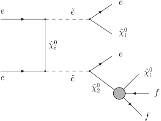
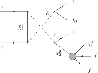
Figure 1: Feynman diagrams for the processes in Eqs. (1). The 4 neutralinos are exchanged in the $t$ channel, and the shaded circles stand for the 8 sub-diagrams mediating the decay of $\tilde{\chi}_{2}^{0}$, separately shown in Fig. 2.

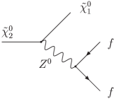
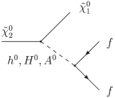
(a)		(b)
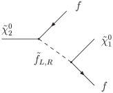
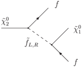
(c)		(d)

Figure 2: Feynman diagrams for the decay of $\tilde{\chi}^{0}_{2}$, mediated by $Z$ bosons (a), neutral Higgs bosons (b), and left-and right-handed scalar fermions (c and d).

The production of mixed $\tilde{e}_{R}\tilde{e}_{L}$ pairs must be taken into account as well, since it constitutes the main background to $\tilde{e}_{L}\tilde{e}_{L}$ and $\tilde{e}_{R}\tilde{e}_{R}$ production in which we are interested. We only consider final states with $f\!\bar{f}=\mu^{+}\mu^{-},q\bar{q}$, and in the case of $q\bar{q}$ we sum $u\bar{u}$, $d\bar{d}$, $s\bar{s}$, $c\bar{c}$ and $b\bar{b}$ production, without flavour tagging. In the channel $\tilde{\chi}_{2}^{0}\to\tilde{\chi}_{1}^{0}e^{+}e^{-}$, the multiplicity of electrons in the final state makes it difficult to identify the electron resulting from the decay of the $\tilde{\chi}_{2}^{0}$. In $\tilde{\chi}_{2}^{0}\to\tilde{\chi}_{1}^{0}\nu\bar{\nu}$ the presence of four undetected particles in the final state yields too many unmeasured momenta for their kinematical determination, and the same happens in $\tilde{\chi}_{2}^{0}\to\tilde{\chi}_{1}^{0}\tau^{+}\tau^{-}$, because each of the $\tau$ leptons decays producing one or two neutrinos that escape detection.

For the generation of the signals we calculate the full matrix elements for the $2\to 6$ resonant processes in Eqs. (1), at a CM energy of 500 GeV and with an integrated luminosity of 100 fb^-1. In the calculation we include the effects of initial state radiation (ISR) and beamstrahlung. We perform a simple simulation of the detector effects with a Gaussian smearing of the energies, applying also phase space cuts on transverse momenta $p_{T}\geq 10$ GeV, pseudorapidities $|\eta|\leq 2.5$ and “lego-plot” separation $\Delta R\geq 0.4$. All the details concerning the generation of the signals can be found in Ref. [2].

For our discussion we restrict ourselves to mSUGRA scenarios, requiring them to be in agreement with present experimental data. We set $m_{1/2}=220$ GeV (in order to have a light spectrum so that these processes are observable with a CM energy of 500 GeV at TESLA), $\tan\beta=10$, $\mu>0$ and for simplicity we choose $A_{0}=0$ (a more extensive discussion is presented in Ref. [2]). The dependence of the studied signals on the remaining parameter $m_{0}$ is shown in Fig. 3.

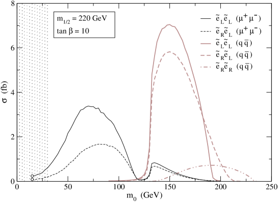
Figure 3: Cross sections (in fb) for $e^{-}e^{-}\to\tilde{e}\tilde{e}\to e^{-}\tilde{\chi}_{1}^{0}e^{-}\tilde{\chi}_{2}^{0}\to e^{-}\tilde{\chi}_{1}^{0}e^{-}\tilde{\chi}_{1}^{0}f\!\bar{f}$ (with unpolarised beams) as a function of $m_{0}$, for $m_{1/2}=220$ GeV, $\tan\beta=10$, $A_{0}=0$ and $\mu>0$.

The shaded area on the left of this plot corresponds to values of $m_{0}$ excluded by the current experimental bounds on $m_{\tilde{e}_{R}}$. In this figure we identify two regions of interest for these signals:

1. For $m_{0}\lesssim 120$ GeV the second neutralino decays predominantly to charged leptons, $\tilde{\chi}_{2}^{0}\to\tilde{\chi}_{1}^{0}l^{+}l^{-}$. The decay amplitudes are dominated by the exchange of on-shell right-handed sleptons (diagrams (c) and (d) in Fig. 2). The contribution of diagram (a) with an on-shell $Z$ boson is less important, due to the smallness of the $Z\tilde{\chi}_{2}^{0}\tilde{\chi}_{1}^{0}$ coupling. In this region of the parameter space, the decays to $\tilde{\chi}_{1}^{0}q\bar{q}$ are very suppressed, not only because of the small coupling of the $Z$ boson to $\tilde{\chi}_{1}^{0}$ and $\tilde{\chi}_{2}^{0}$, but also due to the heavy squark masses, $m_{\tilde{q}}\gtrsim 400$ GeV.

2. For $m_{0}\gtrsim 140$ GeV, the right-handed sleptons (including $\tilde{\tau}_{R}$) are heavier than $\tilde{\chi}_{2}^{0}$, and the $Z$-exchange diagram in Fig. 2 dominates, yielding a large branching ratio for $\tilde{\chi}_{2}^{0}\to\tilde{\chi}_{1}^{0}q\bar{q}$.

Between both regions there is a narrow window $m_{0}\sim 130$ GeV where the decay $\tilde{\chi}_{2}^{0}\to\tilde{\chi}_{1}^{0}\tau^{+}\tau^{-}$ completely dominates, because the $\tilde{e}_{R}$ and $\tilde{\mu}_{R}$ are heavier than the $\tilde{\chi}_{2}^{0}$ but the $\tilde{\tau}_{R}$ is lighter. For $m_{0}\gtrsim 200$ GeV, the production of $\tilde{e}_{L}\tilde{e}_{L}$ and $\tilde{e}_{L}\tilde{e}_{R}$ is not possible with a CM energy of 500 GeV, and only $\tilde{e}_{R}\tilde{e}_{R}$ pairs are produced. From inspection of Fig. 3 we select two values $m_{0}=80$ GeV and $m_{0}=160$ GeV to illustrate the reconstruction of the selectron masses for $\mu^{+}\mu^{-}$ and $q\bar{q}$ final states. The sets of parameters for these two mSUGRA scenarios are summarised in Table 1. The resulting selectron and neutralino masses and widths, as well as the relevant branching ratios, are collected in Table 2 for each of these scenarios.

Parameter		Scenario 1		Scenario 2
$m_{1/2}$		220		220
$m_{0}$		80		160
$A_{0}$		0		0
$\tan\beta$		10		10
$\mathrm{sign}\,\mu$		$+$		$+$

Table 1: Input parameters for the two mSUGRA scenarios to be considered in Section 3. The values of $m_{1/2}$, $m_{0}$ and $A_{0}$ are in GeV.

	Scenario 1		Scenario 2
$m_{\tilde{e}_{L}}$	181.0		227.4
$\Gamma_{\tilde{e}_{L}}$	0.25		0.85
$m_{\tilde{e}_{R}}$	123.0		185.0
$\Gamma_{\tilde{e}_{R}}$	0.17		0.58
$m_{\tilde{\chi}_{1}^{0}}$	84.0		84.3
$m_{\tilde{\chi}_{2}^{0}}$	155.8		156.4
$\Gamma_{\tilde{\chi}_{2}^{0}}$	0.023		$1.50\times 10^{-5}$
$m_{\tilde{\chi}_{3}^{0}}$	309.4		310.0
$\Gamma_{\tilde{\chi}_{3}^{0}}$	1.48		1.43
$m_{\tilde{\chi}_{4}^{0}}$	330.4		331.1
$\Gamma_{\tilde{\chi}_{4}^{0}}$	2.30		2.01
$\mathrm{Br}(\tilde{e}_{L}\to e^{-}\tilde{\chi}_{1}^{0})$	41.8 %		18.3 %
$\mathrm{Br}(\tilde{e}_{L}\to e^{-}\tilde{\chi}_{2}^{0})$	20.6 %		30.8 %
$\mathrm{Br}(\tilde{e}_{R}\to e^{-}\tilde{\chi}_{1}^{0})$	100 %		99.7 %
$\mathrm{Br}(\tilde{e}_{R}\to e^{-}\tilde{\chi}_{2}^{0})$	$\simeq 0$		0.3 %
$\mathrm{Br}(\tilde{\chi}_{2}^{0}\to\tilde{\chi}_{1}^{0}\mu^{+}\mu^{-})$	10.3 %		3.9 %
$\mathrm{Br}(\tilde{\chi}_{2}^{0}\to\tilde{\chi}_{1}^{0}q\bar{q})$	$\simeq 0$		69.2 %

Table 2: Some relevant quantities in the two mSUGRA scenarios considered in Section 3. The masses and widths are in GeV.

It is worth comparing between the $e^{-}\tilde{\chi}_{1}^{0}e^{-}\tilde{\chi}_{2}^{0}$ decay mode studied here and the leading channel $e^{-}\tilde{\chi}_{1}^{0}e^{-}\tilde{\chi}_{1}^{0}$. For $\tilde{e}_{L}\tilde{e}_{L}$ production, in scenario 1 the total branching ratio (including the decay of the $\tilde{\chi}_{2}^{0}$) of the $e^{-}\tilde{\chi}_{1}^{0}e^{-}\tilde{\chi}_{1}^{0}\mu^{+}\mu^{-}$ signal is 0.88%, while for the leading channel it is 17.4%. On the other hand, in scenario 2 the total branching ratio of the $e^{-}\tilde{\chi}_{1}^{0}e^{-}\tilde{\chi}_{1}^{0}q\bar{q}$ signal is 3.9%, slightly larger than for the $e^{-}\tilde{\chi}_{1}^{0}e^{-}\tilde{\chi}_{1}^{0}$ channel. For $\tilde{e}_{R}\tilde{e}_{R}$ production, in scenario 1 the decay $\tilde{e}_{R}\to e^{-}\tilde{\chi}_{2}^{0}$ is not possible because the $\tilde{e}_{R}$ is lighter than the $\tilde{\chi}_{2}^{0}$. In scenario 2, $\mathrm{Br}(\tilde{e}_{R}\to e^{-}\tilde{\chi}_{2}^{0})\simeq 0.3$% because the $\tilde{e}_{R}$ only couples to the small bino component of the second neutralino. The total branching ratios in each case are collected in Table 3.

	Scenario 1		Scenario 2
Final state	$\tilde{e}_{L}\tilde{e}_{L}$	$\tilde{e}_{R}\tilde{e}_{R}$	$\tilde{e}_{L}\tilde{e}_{L}$	$\tilde{e}_{R}\tilde{e}_{R}$
$e^{-}\tilde{\chi}_{1}^{0}e^{-}\tilde{\chi}_{1}^{0}f\!\bar{f}$	0.88%	0	3.9%	0.27%
$e^{-}\tilde{\chi}_{1}^{0}e^{-}\tilde{\chi}_{1}^{0}$	17.4%	100%	3.3%	99%

Table 3: Comparison of the branching ratios for the $e^{-}\tilde{\chi}_{1}^{0}e^{-}\tilde{\chi}_{1}^{0}f\!\bar{f}$ and $e^{-}\tilde{\chi}_{1}^{0}e^{-}\tilde{\chi}_{1}^{0}$ signals in scenarios 1 and 2. In scenario 1, $f\!\bar{f}=\mu^{+}\mu^{-}$, while in scenario 2 $f\!\bar{f}=q\bar{q}$.

3 Reconstruction of the final state and kinematical distributions

To reconstruct the final state momenta we use as input the 4-momenta of the detected particles (the two electrons and the $f\!\bar{f}$ pair), the CM energy and the $\tilde{\chi}_{1}^{0}$ and $\tilde{\chi}_{2}^{0}$ masses, which we assume known from other experiments [1, 3]. In general, it is necessary to have as many kinematical relations as unknown variables in order to determine the momenta of the undetected particles. In our case, there are 8 unknowns (the 4 components of the two $\tilde{\chi}_{1}^{0}$ momenta) and 8 constraints. These are derived from energy and momentum conservation (4 constraints), from the fact that the two $\tilde{\chi}_{1}^{0}$ are on shell (two constraints), from the decay of the $\tilde{\chi}_{2}^{0}$ (one constraint) and from the additional hypothesis that in $e^{-}e^{-}$ scattering two particles of equal mass are produced (one constraint) . These 8 equations determine the 4-momenta of the two $\tilde{\chi}_{1}^{0}$ up to a 4-fold ambiguity, which is partially reduced requiring that the solutions have positive $p_{\tilde{e}}^{2}$ and that the “reconstructed” $m_{\tilde{\chi}_{2}^{0}}^{\mathrm{rec}}$ is similar to the real value . If none of the four solutions passes these conditions the event is discarded, otherwise from the remaining solutions we select the one giving the smallest $m_{\tilde{e}}$. For $\mu^{+}\mu^{-}$ final states this is the best choice: for the events where the two selectrons are nearly on-shell (these events give the main contribution to the cross section) the solution with smallest $m_{\tilde{e}}$ is the “correct” one 65% of the time, and provides a very good reconstruction of the selectron and $\tilde{\chi}_{2}^{0}$ rest frames. The (discarded) solution with largest $m_{\tilde{e}}$ gives a bad $\tilde{\chi}_{2}^{0}$ 4-momentum, and leads to large distortions for the angular distributions in the $\tilde{\chi}_{2}^{0}$ rest frame. For $q\bar{q}$ final states the solution with smallest $m_{\tilde{e}}$ gives the best reconstruction as well, but the difference with the other solution is not so important.

It is worthwhile remarking here that ISR, beamstrahlung, particle width effects and detector resolution degrade the determination of the $\tilde{\chi}_{1}^{0}$ momenta. However, the reconstruction is successfully achieved in most cases. The reconstruction procedure determines the momenta of the two unobserved $\tilde{\chi}_{1}^{0}$, identifying which selectron has decayed to $e^{-}\tilde{\chi}_{1}^{0}$ and which to $e^{-}\tilde{\chi}_{2}^{0}$, and also distinguishes between the electrons resulting from each of these decays. The knowledge of all the final state momenta, as well as the identification of the particles resulting from each decay, allows to construct various mass, angular and energy distributions. These are discussed in turn.

3.1 Mass distributions

Let us call “$e^{-}_{1}$” and “$\tilde{\chi}_{1,1}^{0}$” the particles resulting from $\tilde{e}\to e^{-}\tilde{\chi}_{1}^{0}$, with “$\tilde{e}_{1}$” the corresponding selectron, and analogously “$e^{-}_{2}$”, “$\tilde{\chi}_{1,2}^{0}$” and “$\tilde{e}_{2}$” the particles involved in $\tilde{e}\to e^{-}\tilde{\chi}_{2}^{0}$. The reconstructed mass of the selectrons is simply

$$m_{\tilde{e}}\equiv\sqrt{p_{\tilde{e}_{1}}^{2}}=\sqrt{p_{\tilde{e}_{2}}^{2}}\,,$$ (2)

with

$$p_{\tilde{e}_{1}} \equiv p_{e_{1}^{-}}+p_{\tilde{\chi}_{1,1}^{0}}\,,$$

$$p_{\tilde{e}_{2}} \equiv p_{e_{2}^{-}}+p_{\tilde{\chi}_{1,2}^{0}}+p_{f}+p_{\bar{f}}$$ (3)

in obvious notation. All these momenta are taken in the laboratory frame. The distribution of this variable for the $\tilde{e}_{L}\tilde{e}_{L}$ and $\tilde{e}_{R}\tilde{e}_{R}$ signals and the $\tilde{e}_{R}\tilde{e}_{L}$ background is shown in Fig. 4. In these and the rest of plots we represent cross sections; the number of observed events depends on the luminosity and is subject to statistical fluctuations. For the generation of the distributions we have taken sufficiently high statistics so as to have a small Monte Carlo uncertainty.

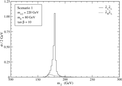
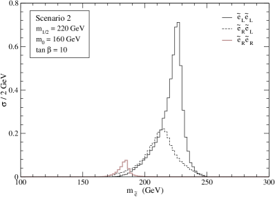
Figure 4: Reconstructed selectron mass in scenarios 1 and 2, for unpolarised beams.

As seen from Fig. 4, the reconstruction of the masses is quite effective. For $\tilde{e}_{L}\tilde{e}_{L}$ production, a peak around the true $\tilde{e}_{L}$ mass ($m_{e_{L}}=181$ GeV in scenario 1, $m_{e_{L}}=227$ GeV in scenario 2) is observed in each scenario. (The peak is sharper in scenario 1 due to the better energy resolution for muons than for jets and the smaller $\tilde{e}_{L}$ width.) For $\tilde{e}_{R}\tilde{e}_{R}$ production in scenario 2, a tiny peak is observed around the true $\tilde{e}_{R}$ mass $m_{e_{R}}=185$ GeV. The $\tilde{e}_{R}\tilde{e}_{L}$ background is suppressed by the reconstruction procedure in both scenarios. In scenario 1, its distribution is approximately flat, but in scenario 2 it noticeably concentrates around $215$ GeV. This behaviour is a result of the smaller ratio $(m_{\tilde{e}_{L}}-m_{\tilde{e}_{R}})/(m_{\tilde{e}_{L}}+m_{\tilde{e}_{R}})$: in scenario 2, the hypothesis of two particles produced with equal mass, used for the reconstruction, becomes more accurate. The cross sections of the three processes, before and after the reconstruction, are collected in Table 4. We also include the cross sections for polarised beams, in order to show how the $\tilde{e}_{L}\tilde{e}_{L}$ and $\tilde{e}_{R}\tilde{e}_{R}$ signals can be enhanced with negative and positive beam polarisation, respectively, while the $\tilde{e}_{R}\tilde{e}_{L}$ background is reduced in both cases.

	Scenario 1					Scenario 2
	$P_{00}$		$P_{--}$			$P_{00}$		$P_{--}$		$P_{++}$
	before	after	before	after		before	after	before	after	before	after
$\tilde{e}_{L}\tilde{e}_{L}$	3.25	2.88	10.52	9.32		6.52	5.71	21.14	18.50	0.26	0.23
$\tilde{e}_{R}\tilde{e}_{R}$	–	–	–	–		0.41	0.34	0.02	0.01	1.34	1.10
$\tilde{e}_{R}\tilde{e}_{L}$	1.66	0.47	0.60	0.17		5.41	2.63	1.95	0.95	1.95	0.95

Table 4: Cross sections (in fb) for selectron pair production and subsequent decay in scenarios 1 and 2. We quote results before and after reconstruction, for unpolarised beams ($P_{00}$), for $P_{1}=P_{2}=-0.8$ ($P_{--}$) and in scenario 2 also for $P_{1}=P_{2}=0.8$ ($P_{++}$). Detector cuts are included in all cases.

The experimental measurement of the selectron masses from these distributions is less precise than from threshold scans [4, 5]. These mass distributions are however useful in order to identify $\tilde{e}_{L}\tilde{e}_{L}$ and $\tilde{e}_{R}\tilde{e}_{R}$ production, and may be used to separate them from the $\tilde{e}_{R}\tilde{e}_{L}$ background. We also note that in the $e^{-}\tilde{\chi}_{1}^{0}e^{-}\tilde{\chi}_{1}^{0}$ channel, even without a complete determination of the final state momenta the minimum kinematically allowed selectron mass can be obtained [6]. The kinematical distribution of this quantity also peaks at the true selectron masses.

3.2 Production angle

The determination of the selectron momenta allows the study of the dependence of the cross section on the production angle $\theta$. In $e^{+}e^{-}$ scattering, this analysis can be used to determine that the selectrons are spinless particles [1] . In our case, it does not provide information about the selectron spins. This distribution, shown in Fig. 5 for both scenarios, is symmetric with respect to the value $\cos\theta=0$, as must be for a process with a symmetric initial state $e^{-}e^{-}$, and follows the expected shape.

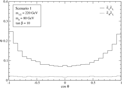
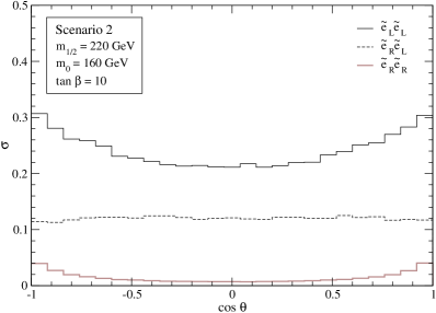
Figure 5: Dependence of the cross section on the production angle $\theta$ in scenarios 1 and 2, for unpolarised beams.

3.3 Electron angular distributions in selectron rest frames

The selectron spins can be effectively analised through the angular distributions of the electrons in the selectron rest frames. Since the selectrons are spinless particles, their decay is isotropic. Therefore in each selectron rest frame the angular distribution of the produced electron (and neutralino) with respect to any fixed direction must be flat. In Fig. 6 we show the dependence of the cross section on the angle $\theta_{1}$ between the momentum of $e_{1}^{-}$ in the $\tilde{e}_{1}$ rest frame and the positive $y$ axis (remember that $e_{1}^{-}$ and $\tilde{e}_{1}$ correspond to the decay $\tilde{e}\to e^{-}\tilde{\chi}_{1}^{0}$, and are identified in the reconstruction process). The analogous is shown for the decay $\tilde{e}\to e^{-}\tilde{\chi}_{2}^{0}$ in Fig. 7, with $\theta_{2}$ the angle between the momentum of $e_{2}^{-}$ and the positive $y$ axis. Similar distributions can be obtained for the $x$ and $z$ axes, proving that the decay of both selectrons is isotropic.

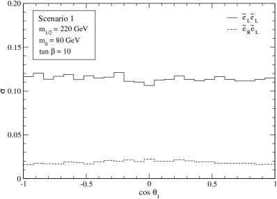
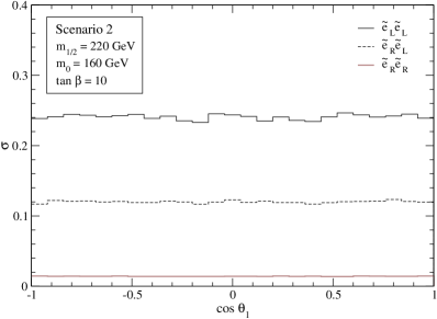
Figure 6: Angular distribution of $e_{1}^{-}$ with respect to the positive $y$ axis in the $\tilde{e}_{1}$ rest frame, in scenarios 1 and 2, for unpolarised beams.

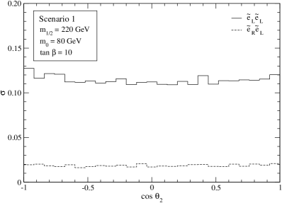
Figure 7: Angular distribution of $e_{2}^{-}$ with respect to the positive $y$ axis in the $\tilde{e}_{2}$ rest frame, in scenarios 1 and 2, for unpolarised beams.

3.4 Electron energy distributions in laboratory frame

The masses and spins of the selectrons can be further investigated via the electron energy distributions. In the selectron rest frame, the electron energy is fixed by the kinematics of the 2-body decay, and furthermore their decay is isotropic. Then, for $\tilde{e}_{L}\tilde{e}_{L}$ and $\tilde{e}_{R}\tilde{e}_{R}$ production the electron energy distributions are flat, with end points at

$$E_{i}^{\mathrm{max}} = \frac{\sqrt{s}}{4}\left(1-\frac{m_{\tilde{\chi}_{i}^{0}}^{2}}{m_{\tilde{e}_{L,R}}^{2}}\right)(1+\beta)\;,$$

$$E_{i}^{\mathrm{min}} = \frac{\sqrt{s}}{4}\left(1-\frac{m_{\tilde{\chi}_{i}^{0}}^{2}}{m_{\tilde{e}_{L,R}}^{2}}\right)(1-\beta)\;,$$ (4)

where $\beta=\sqrt{1-4m_{\tilde{e}_{L,R}}^{2}/s}$. For mixed selectron production the electron energy spectra are flat as well, but the expressions of the end points are more involved. In contrast with the decay mode $e^{-}\tilde{\chi}_{1}^{0}e^{-}\tilde{\chi}_{1}^{0}$, in the channel $e^{-}\tilde{\chi}_{1}^{0}e^{-}\tilde{\chi}_{2}^{0}$ there are two different distributions for the energies $E_{1}$ and $E_{2}$ of the electrons $e_{1}^{-}$ and $e_{2}^{-}$, respectively. The distribution of $E_{1}$ in both scenarios is shown in Fig. 8. From Eqs. 4, in scenario 1 the expected end points are $E_{1}^{\mathrm{min}}=30$ GeV, $E_{1}^{\mathrm{max}}=166$ GeV. In scenario 2, for $\tilde{e}_{L}$ decays the expected limits of the distributions are $E_{1}^{\mathrm{min}}=63$ GeV, $E_{1}^{\mathrm{max}}=153$ GeV, and for $\tilde{e}_{R}$ decays they are $E_{1}^{\mathrm{min}}=32$ GeV, $E_{1}^{\mathrm{max}}=166$ GeV. Although the distributions are smeared by ISR, beamstrahlung and detector effects, all these end points can be clearly observed in the plots. However, in the real experiment the different contributions will be summed, and except in some cases where the end points coincide, in general beam polarisation will be essential in order to enhance one of the signals and reduce the $\tilde{e}_{R}\tilde{e}_{L}$ background. The polarisation also improves the statistics and thus the acuracy of the end point determination. The measurement of these quantities gives further evidence that the selectrons are spinless particles and provides independent determinations of their masses.

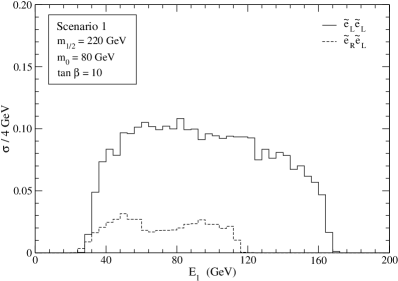
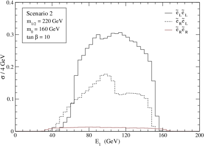
Figure 8: Energy distribution of the electron resulting from $\tilde{e}\to e^{-}\tilde{\chi}_{1}^{0}$, in scenarios 1 and 2, for unpolarised beams.

For the decays $\tilde{e}\to e^{-}\tilde{\chi}_{2}^{0}$, the corresponding electron energy distribution is shown in Fig. 9. In scenario 1, the expected limits are $E_{2}^{\mathrm{min}}=10$ GeV, $E_{2}^{\mathrm{max}}=55$ GeV. In scenario 2, for $\tilde{e}_{L}$ decays the expected end points are $E_{2}^{\mathrm{min}}=38$ GeV, $E_{2}^{\mathrm{max}}=93$ GeV and for $\tilde{e}_{R}$ decays they are $E_{2}^{\mathrm{min}}=12$ GeV, $E_{2}^{\mathrm{max}}=60$ GeV. All these end points can be observed in Fig. 9.

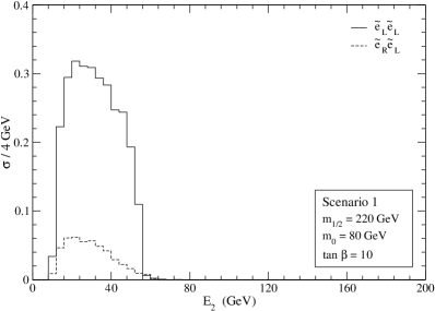
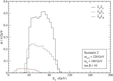
Figure 9: Energy distribution of the electron resulting from $\tilde{e}\to e^{-}\tilde{\chi}_{2}^{0}$, in scenarios 1 and 2, for unpolarised beams.

3.5 Distributions in $\boldsymbol{\tilde{\chi}_{2}^{0}}$ rest frame

The neutralinos resulting from selectron decay are 100% polarised in the direction of their momentum if selectron mixing is neglected. This fact can be explained as follows. The term of the Lagrangian describing $e\tilde{e}\tilde{\chi}_{i}^{0}$ interactions is, neglecting selectron mixing,

$$\mathcal{L}_{e\tilde{e}\tilde{\chi}_{i}^{0}}=a_{L}^{i}\;\tilde{e}_{L}^{*}\,\bar{\tilde{\chi}}_{i}^{0}P_{L}\,e+a_{L}^{i*}\;\tilde{e}_{L}\,\bar{e}\,P_{R}\,\tilde{\chi}_{i}^{0}+a^{i}_{R}\;\tilde{e}_{R}^{*}\,\bar{\tilde{\chi}}_{j}^{0}P_{R}\,e+a_{R}^{i*}\;\tilde{e}_{R}\,\bar{e}\,P_{L}\,\tilde{\chi}_{i}^{0}\,,$$ (5)

with $a_{L}^{i}$ and $a_{R}^{i}$ constants. For $\tilde{e}_{L}\to e^{-}\tilde{\chi}_{i}^{0}$, the produced electron has chirality $-1$, and the neutralino has chirality $+1$. For a massive particle, the helicity eigenstates do not coincide in general with the chirality eigenstates. However, since in this case the helicity of the electron is $-1$ and the selectron is spinless, angular momentum conservation implies that the neutralino must have negative helicity, as shown schematically in Fig. 10a. For $\tilde{e}_{R}$ decays, the same argument shows that the produced neutralinos have positive helicity (Fig. 10b)

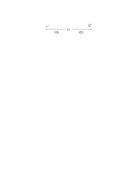
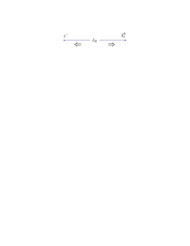
(a)		(b)

Figure 10: Helicity of the neutralinos produced in $\tilde{e}_{L}$ and $\tilde{e}_{R}$ decays.

The expressions of the polarised differential decay widths of $\tilde{\chi}_{2}^{0}\to\tilde{\chi}_{1}^{0}f\!\bar{f}$ are rather involved [8, 9, 10]. However, the angular distribution of a single decay product in the $\tilde{\chi}_{2}^{0}$ rest frame can be cast in a very compact form. Let us define $\psi_{+}$, $\psi_{-}$ and $\psi_{0}$ as the polar angles between the 3-momenta in the $\tilde{\chi}_{2}^{0}$ rest frame of $\bar{f}=\mu^{+},\bar{q}$, $f=\mu^{-},q$ and $\tilde{\chi}_{1}^{0}$, respectively, and the $\tilde{\chi}_{2}^{0}$ spin $\vec{s}$. These angles are represented in Fig. 11.

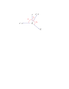
Figure 11: Definition of the polar angles $\psi_{+}$, $\psi_{-}$ and $\psi_{0}$.

Integrating all the variables except $\psi_{+}$, $\psi_{-}$ or $\psi_{0}$, the angular decay distributions can be written as

$$\frac{1}{\sigma}\frac{d\sigma}{d\cos\psi_{+}} = \frac{1+h^{f}_{+}\cos\psi_{+}}{2}\,,$$

$$\frac{1}{\sigma}\frac{d\sigma}{d\cos\psi_{-}} = \frac{1+h^{f}_{-}\cos\psi_{-}}{2}\,,$$

$$\frac{1}{\sigma}\frac{d\sigma}{d\cos\psi_{0}} = \frac{1+h^{f}_{0}\cos\psi_{0}}{2}\,.$$ (6)

The constants $h_{i}^{f}$ depend on the type of fermion $f=\mu,u,d,s,c,b$ considered (and of course on the SUSY scenario), and measure the degree of correlation between the $\tilde{\chi}_{2}^{0}$ spin and the direction in which the fermion $f$ is emitted. If CP is conserved in this decay, the Majorana nature of $\tilde{\chi}_{1}^{0}$ and $\tilde{\chi}_{2}^{0}$ implies that $h_{+}^{f}=-h_{-}^{f}$ and $h_{0}^{f}=0$. In scenario 1, $h_{+}^{\mu}=-h_{-}^{\mu}=-0.57$, and in scenario 2 we find $h_{+}^{b}=-h_{-}^{b}=0.75$.

The fact that the $\tilde{\chi}_{2}^{0}$ produced in $\tilde{e}$ decays are polarised allows the study of angular distributions in the $\tilde{\chi}_{2}^{0}$ rest frame. In analogy with Fig. 11, we define the polar angles $\varphi_{+}$, $\varphi_{-}$ and $\varphi_{0}$ between the 3-momenta in the $\tilde{\chi}_{2}^{0}$ rest frame of $\bar{f}$, $f$ and $\tilde{\chi}_{1}^{0}$, respectively, and the 3-momentum $\vec{p}$ of $\tilde{\chi}_{2}^{0}$ in the $\tilde{e}_{2}$ rest frame. (In $\tilde{e}_{R}$ decays, $\vec{p}$ gives the direction of the spin $\tilde{s}$, and in $\tilde{e}_{L}$ decays the opposite direction.) With these definitions, we build the spin asymmetries

$$A_{i}\equiv\frac{N(\cos\varphi_{i}>0)-N(\cos\varphi_{i}<0)}{N(\cos\varphi_{i}>0)+N(\cos\varphi_{i}<0)}\,,$$ (7)

where $N$ stands for the number of events. The theoretical prediction for these asymmetries is $A_{i}=\lambda\,h_{i}^{f}/2$, with $\lambda$ the helicity of $\tilde{\chi}_{2}^{0}$.

Figure 12: Definition of the polar angles $\varphi_{+}$, $\varphi_{-}$ and $\varphi_{0}$.

The angular distributions of $\mu^{+}$ and $\mu^{-}$ in scenario 1 are presented in Fig. 13, for the $\tilde{e}_{L}\tilde{e}_{L}$ signal and the $\tilde{e}_{R}\tilde{e}_{L}$ background. In both cases we observe a suppression at $\cos\varphi_{\pm}=-1$, due to the detector cuts. For $\cos\varphi_{\pm}=-1$, the $\mu^{\pm}$ is emitted in the direction of $-\vec{p}$, which is the direction of the $e^{-}_{2}$, thus these two particles are not isolated and the event is rejected by the requirement on “lego-plot” separation.

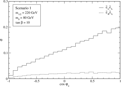
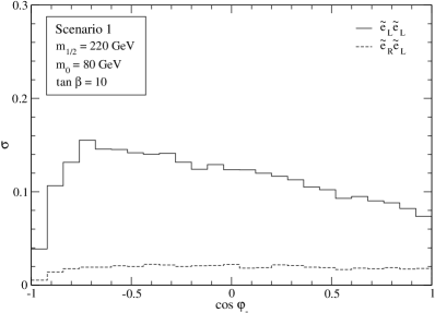
Figure 13: Angular distribution of the $\mu^{+}$ and $\mu^{-}$ in the $\tilde{\chi}_{2}^{0}$ rest frame with respect to the $\tilde{\chi}_{2}^{0}$ momentum in the $\tilde{e}_{2}$ rest frame, in scenario 1.

The slopes of these distributions clearly show that the $\tilde{\chi}_{2}^{0}$ has helicity $-1$ ($h_{+}^{\mu}=-0.57$ in this scenario) and hence that the decaying selectron is a $\tilde{e}_{L}$. This information can be of course obtained from other sources, for instance with the comparison of production cross sections with and without polarisation. Additionally, these plots demonstrate that the $\tilde{\chi}_{2}^{0}$ has nonzero spin (compare with $\tilde{e}$ decays in Figs. 6 and 7). For $\tilde{e}_{L}\tilde{e}_{L}$ production only , the asymmetries are $A_{+}=0.39$, $A_{-}=-0.12$, while the theoretical expectations are $A_{\pm}=\pm 0.29$.

In scenario 2, the experimental measurement of these asymmetries requires to distinguish $q$ from $\bar{q}$. This is very difficult to do in general, so we restrict ourselves to $q=b$ where this is possible although with a limited efficiency. The angular distributions of the $\bar{b}$ ($\varphi_{+}$) and $b$ ($\varphi_{-}$) are shown in Fig. 14. In these plots we have not taken into account neither efficiencies nor mistagging rates for the $b,\bar{b}$ identification.

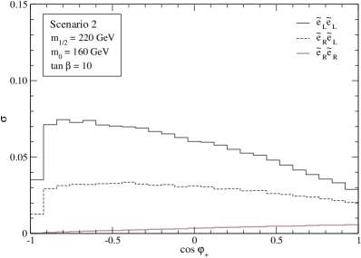
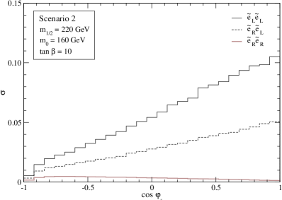
Figure 14: Angular distribution of the $\bar{b}$ ($\varphi_{+}$) and $b$ ($\varphi_{-}$)in the $\tilde{\chi}_{2}^{0}$ rest frame with respect to the $\tilde{\chi}_{2}^{0}$ momentum in the $\tilde{e}_{2}$ rest frame, in scenario 2.

The slope of the angular distribution for the $\tilde{e}_{L}\tilde{e}_{L}$ signal again shows that the $\tilde{\chi}_{2}^{0}$ has negative helicity ($h_{+}^{b}=0.75$ in this scenario), and thus indicates that the decaying selectron is a $\tilde{e}_{L}$. The asymmetries for this process alone are $A_{+}=-0.15$, $A_{-}=0.41$, and the theoretical predictions $A_{\pm}=\mp 0.37$. For $\tilde{e}_{R}\tilde{e}_{R}$, the positive slope indicates a decay from a $\tilde{e}_{R}$, and the asymmetries in this case are $A_{+}=0.39$, $A_{-}=-0.21$. The $\tilde{e}_{R}\tilde{e}_{R}$ signal could in principle be observable with positive beam polarisation, which increases its cross section by a factor of 3.24 and reduces $\tilde{e}_{L}\tilde{e}_{L}$ and $\tilde{e}_{R}\tilde{e}_{L}$ by factors of 0.04 and 0.36, respectively (see Table 4). In addition, kinematical cuts on reconstructed masses could be applied to enhance $\tilde{e}_{R}\tilde{e}_{R}$ (see Fig. 4).

4 Conclusions

In this note we have analysed $\tilde{e}_{L}\tilde{e}_{L}$ and $\tilde{e}_{R}\tilde{e}_{R}$ production in $e^{-}e^{-}$ collisions, with subsequent decay $\tilde{e}\tilde{e}\to e^{-}\tilde{\chi}_{1}^{0}e^{-}\tilde{\chi}_{2}^{0}\to e^{-}\tilde{\chi}_{1}^{0}e^{-}\tilde{\chi}_{1}^{0}f\!\bar{f}$. For $\tilde{e}_{R}\tilde{e}_{R}$ production, this is a rare channel, with a cross section much smaller than the leading mode $e^{-}\tilde{\chi}_{1}^{0}e^{-}\tilde{\chi}_{1}^{0}$, but for $\tilde{e}_{L}\tilde{e}_{L}$ it may have a comparable or even larger cross section. We have shown some of the benefits that the reconstruction of all the final state momenta offers, allowing the study of mass, angular and energy distributions.

We have demonstrated that in this decay mode it is possible to gather information on the $\tilde{\chi}_{2}^{0}$ spin, what is not possible in $e^{-}\tilde{\chi}_{1}^{0}e^{-}\tilde{\chi}_{1}^{0}$ decays. This is of special interest since in selectron decays the neutralinos are 100% polarised, having negative helicity (in the selectron rest frame) in $\tilde{e}_{L}$ decays and positive helicity in $\tilde{e}_{R}$ decays. Indeed, $\tilde{e}_{L}$ decays are a source of 100% polarised $\tilde{\chi}_{2}^{0}$ with a cross section comparable or even larger than direct production $e^{+}e^{-}\to\tilde{\chi}_{1}^{0}\tilde{\chi}_{2}^{0}$. In this work we have used the distribution of the $\tilde{\chi}_{2}^{0}$ decay products only to distinguish $\tilde{e}_{L}$ from $\tilde{e}_{R}$, but $\tilde{\chi}_{2}^{0}$ decays also offer a good place to investigate CP violation in the neutralino sector [11] through the analysis of CP-violating asymmetries [12]. This study will be presented elsewhere [13].

Acknowledgements

I thank A. M. Teixeira for previous collaboration. This work has been supported by the European Community’s Human Potential Programme under contract HTRN–CT–2000–00149 Physics at Colliders and by FCT through project CFIF–Plurianual (2/91) and grant SFRH/BPD/12603/2003.

References

- [1] J. A. Aguilar-Saavedra et al. [ECFA/DESY LC Physics Working Group Collaboration], hep-ph/0106315
- [2] J. A. Aguilar-Saavedra and A. M. Teixeira, Nucl. Phys. B 675, 70 (2003) [hep-ph/0307001]
- [3] H. U. Martyn and G. A. Blair, hep-ph/9910416
- [4] J. L. Feng and M. E. Peskin, Phys. Rev. D 64, 115002 (2001) [hep-ph/0105100]
- [5] C. Blochinger, H. Fraas, G. Moortgat-Pick and W. Porod, Eur. Phys. J. C 24, 297 (2002) [hep-ph/0201282]
- [6] J. L. Feng and D. E. Finnell, Phys. Rev. D 49, 2369 (1994) [hep-ph/9310211]
- [7] H. U. Martyn, hep-ph/0002290
- [8] G. Moortgat-Pick, H. Fraas, A. Bartl and W. Majerotto, Eur. Phys. J. C 9, 521 (1999) [Erratum-ibid. C 9, 549 (1999)] [hep-ph/9903220]
- [9] S. Y. Choi, H. S. Song and W. Y. Song, Phys. Rev. D 61, 075004 (2000) [hep-ph/9907474]
- [10] A. Djouadi, Y. Mambrini and M. Mühlleitner, Eur. Phys. J. C 20, 563 (2001) [hep-ph/0104115]
- [11] See for instance J. Kalinowski, Acta Phys. Polon. B 34, 3441 (2003) [hep-ph/0306272]. For the reconstruction of CP-violating quantities from CP-conserving observables, see S. Y. Choi, J. Kalinowski, G. Moortgat-Pick and P. M. Zerwas, Eur. Phys. J. C 22, 563 (2001) [Addendum-ibid. C 23, 769 (2002)] [hep-ph/0108117]
- [12] A. Bartl, H. Fraas, O. Kittel and W. Majerotto, hep-ph/0308141
- [13] J. A. Aguilar-Saavedra, hep-ph/0403243, to be published in Phys. Lett. B